i

NAVAL POSTGRADUATE SCHOOL Monterey, California

THESIS

Approved for public release; distribution is unlimited

ANALYSIS OF A SEMI-TAILLESS AIRCRAFT DESIGN

by

Kurt W. Muller

March 2002

Thesis Advisor: Conrad F. Newberry Second Reader: Richard M. Howard

ii

THIS PAGE INTENTIONALLY LEFT BLANK

i

REPORT DOCUMENTATION PAGE Form Approved OMB No. 0704-0188

Public reporting burden for this collection of information is estimated to average 1 hour per response, including the time for reviewing instruction, searching existing data sources, gathering and maintaining the data needed, and completing and reviewing the collection of information. Send comments regarding this burden estimate or any other aspect of this collection of information, including suggestions for reducing this burden, to Washington headquarters Services, Directorate for Information Operations and Reports, 1215 Jefferson Davis Highway, Suite 1204, Arlington, VA 22202-4302, and to the Office of Management and Budget, Paperwork Reduction Project (0704-0188) Washington DC 20503. 1. AGENCY USE ONLY (Leave blank)

2. REPORT DATE March 2002

3. REPORT TYPE AND DATES COVERED Master’s Thesis

4. TITLE AND SUBTITLE: Title (Mix case letters) Analysis of a Semi-Tailles Aircraft Design 6. AUTHOR(S) LT Kurt Muller

5. FUNDING NUMBERS

7. PERFORMING ORGANIZATION NAME(S) AND ADDRESS(ES) Naval Postgraduate School Monterey, CA 93943-5000

8. PERFORMING ORGANIZATION REPORT NUMBER

9. SPONSORING / MONITORING AGENCY NAME(S) AND ADDRESS(ES) N/A

10. SPONSORING / MONITORING AGENCY REPORT NUMBER

11. SUPPLEMENTARY NOTES The views expressed in this thesis are those of the author and do not reflect the official policy or position of the Department of Defense or the U.S. Government. 12a. DISTRIBUTION / AVAILABILITY STATEMENT Approved for public release; distribution is unlimited

12b. DISTRIBUTION CODE

13. ABSTRACT (maximum 200 words)

Many unique aircraft configurations came out of Germany in World War II, one of these was the Blohm and Voss BV P 208. By using longitudinal and directional control surfaces located outboard of the wing tips they are removed from the downwash of the main wing. Additionally, the result is fewer component surfaces with less total surface area, thereby reducing both friction and interference drag and manufacturing cost.

The configuration should lend itself well to low-observability, making it a good stealth candidate.

The P 208, provided the author an opportunity to analyze an unconventional configuration with the conceptual NASA design codes RAM, VORVIEW, and ACSYNT. A lack of wind tunnel or flight data prevented the evaluation of the performance of these codes for this configuration. However, results are presented for future comparison and evaluation.

Claims of aerodynamic benefits of the P 208 configuration appear largely to be verified. The P 208 suffers from poor natural short-period longitudinal stability and an unstable Dutch-roll, neither of which are beyond the means of artificial control. The most immediate need for future work is a structural analysis and determination as to the structural and dynamic feasibility of the configuration.

15. NUMBER OF PAGES

108

14. SUBJECT TERMS Semi-tailless, P 208, RAM, VORVIEW, ACSYNT

16. PRICE CODE

17. SECURITY CLASSIFICATION OF REPORT

Unclassified

18. SECURITY CLASSIFICATION OF THIS PAGE

Unclassified

19. SECURITY CLASSIFICATION OF ABSTRACT

Unclassified

20. LIMITATION OF ABSTRACT

UL

NSN 7540-01-280-5500 Standard Form 298 (Rev. 2-89) Prescribed by ANSI Std. 239-18

ii

THIS PAGE INTENTIONALLY LEFT BLANK

iii

Approved for public release; distribution is unlimited

ANALYSIS OF A SEMI-TAILLESS AIRCRAFT DESIGN

Kurt W. Muller Lieutenant, United States Navy

B.S., U.S. Naval Academy, 1993

Submitted in partial fulfillment of the requirements for the degree of

MASTER OF SCIENCE IN AERONAUTICAL ENGINEERING

from the

NAVAL POSTGRADUATE SCHOOL March 2002

Author: Kurt W. Muller

Approved by: Conrad F. Newberry, Thesis Advisor

Richard Howard, Second Reader

Max Platzer, Chairman Department of Aeronautics and Astronautics

iv

THIS PAGE INTENTIONALLY LEFT BLANK

v

ABSTRACT

Many unique aircraft configurations came out of Germany in World War II, one

of these was the Blohm and Voss BV P 208. By using longitudinal and directional

control surfaces located outboard of the wing tips they are removed from the downwash

of the main wing. Additionally, the result is fewer component surfaces with less total

surface area, thereby reducing both friction and interference drag and manufacturing cost.

The configuration should lend itself well to low-observability, making it a good

stealth candidate.

The P 208 provided the author an opportunity to analyze an unconventional

configuration with the conceptual NASA design codes RAM, VORVIEW, and

ACSYNT. A lack of wind tunnel or flight data prevented the evaluation of the

performance of these codes for this configuration. However, results are presented for

future comparison and evaluation.

Claims of aerodynamic benefits of the P 208 configuration appear largely to be

verified. The P 208 suffers from poor natural short-period longitudinal stability and an

unstable Dutch-roll, neither of which are beyond the means of artificial control. The

most immediate need for future work is a structural analysis and determination as to the

structural and dynamic feasibility of the configuration.

vi

THIS PAGE INTENTIONALLY LEFT BLANK

vii

TABLE OF CONTENTS

I. INTRODUCTION........................................................................................................1 A. BACKGROUND ..............................................................................................1 B. PURPOSE OF THE STUDY..........................................................................2 C. NASA DESIGN CODES..................................................................................2 D. CONFIGURATION THEORY ......................................................................5

II. P 208 COMPUTER MODEL DEVELOPMENT ...................................................11 A. P 208 MODEL DEVELOPMENT................................................................11

1. Basic P 208 Parameters .....................................................................11 2. Flight Conditions ................................................................................17

III. P208 PERFORMANCE.............................................................................................19

IV. STABILITY AND CONTROL.................................................................................25 A. ELEVATOR TRIM .......................................................................................25 B. LONGITUDINAL STABILITY...................................................................26 C. LATERAL-DIRECTIONAL STABILITY .................................................32 D. FLYING QUALITIES ...................................................................................37

V. CONCLUSIONS AND RECCOMENDATIONS....................................................39 A. CONCLUSIONS ............................................................................................39

1. Configuration Suitability...................................................................39 2. NASA codes ........................................................................................39

B. RECCOMMENDATIONS............................................................................41

LIST OF REFERENCES ......................................................................................................43

APPENDIX A: WEIGHTS ...................................................................................................45

APPENDIX B: EXAMPLE BV PERFORMANCE DATA ...............................................47

APPENDIX C: VORVIEW PRODUCTS............................................................................51

APPENDIX D: DIMENSIONAL STABILITY DERIVATIVES ......................................55

APPENDIX E: MATLAB CODE.........................................................................................59

APPENDIX F: RAM FILE ...................................................................................................65

APPENDIX G: ACSYNT......................................................................................................73

INITIAL DISTRIBUTION LIST.........................................................................................89

viii

THIS PAGE INTENTIONALLY LEFT BLANK

ix

LIST OF FIGURES

Figure 1. BV P 208.03 3-View [After: Ref. 2] .................................................................1 Figure 2. Rapid Aircraft Modeler ......................................................................................3 Figure 3. VORVIEW Example ..........................................................................................4 Figure 4. Outboard Horizontal Stabilizer Configuration [From: Ref. 7] ..........................6 Figure 5. Upwash Flow Angle Over Horizontal Stablizer [From: Ref. 10]......................7 Figure 6. Alliance I............................................................................................................8 Figure 7. Example of Primary Blohm and Voss Data [From: Ref. 12]...........................11 Figure 8. Engine Power vs. Altitude [From: Ref. 12] .....................................................13 Figure 9. Drag Polar Build Up [From: Ref. 12] ..............................................................14 Figure 10. Drag Study on the XP-41 [From: Ref. 15].......................................................16 Figure 11. P 208 1 G Performance Envelope [After: Ref. 12]..........................................17 Figure 12. Span Efficiency vs. Lift Coefficient ................................................................20 Figure 13. P 208 Spanloading ...........................................................................................20 Figure 14. Spanloading with Aileron Deflection ..............................................................21 Figure 15. P 208 Lift Curve ...............................................................................................22 Figure 16. Drag Polar Comparison....................................................................................23 Figure 17. P 208 Drag Polar..............................................................................................23 Figure 18. Coordinate Sign Convention [From: Ref. 17]..................................................27 Figure 19. Static Stability..................................................................................................27 Figure 20. Short-Period Response to Initial Condition.....................................................30 Figure 21. Long-Period Response to Initial Condition .....................................................31 Figure 22. Longitudinal Response to Elevator Step Input ................................................32 Figure 23. Dutch-Roll Response to Initial Condition........................................................35 Figure 24. Roll mode Response to Initial Condition.........................................................36 Figure 25. Spiral mode Response to Initial Condition......................................................37 Figure 26. Original Weights Data [From: Ref. 12] ...........................................................45

x

THIS PAGE INTENTIONALLY LEFT BLANK

xi

LIST OF TABLES

Table 1. Technical Data .................................................................................................12 Table 2. Moments of Inertia (slug ft2)............................................................................14 Table 3. Flight Conditions .............................................................................................17 Table 4. P 208 L/D.........................................................................................................24 Table 5. Approach Configuration Trim .........................................................................25 Table 6. Trimmed Conditions ........................................................................................26 Table 7. Longitudinal Roots...........................................................................................29 Table 8. Lateral-Directional Roots.................................................................................34 Table 9. Sea-level Performance Data [From: Ref. 12]...................................................47 Table 10. High Power Sea- level Performance [From: Ref. 12] .......................................48 Table 11. High Altitude Performance [From: Ref. 12] ....................................................49 Table 12. High Altitude High Power Performance [From: Ref.12].................................50 Table 13. Dimensional Derivative Description [Ref. 17] ................................................55 Table 14. P 208 Dimensional Derivatives .......................................................................56

xii

THIS PAGE INTENTIONALLY LEFT BLANK

xiii

LIST OF SYMBOLS AND ABBREVIATIONS

a, AOA Angle of Attack

ß Sideslip

d Control deflection, subscript ‘e’ for elevator and ‘a’ for aileron

e downwash angle (positive downwards)

? Damping ratio

? Pitch angle

? Roots of quadratic equation (characteristic equation)

f Roll angle

? n Natural frequency

AR Aspect Ratio; b2/S

AC Aerodynamic Center

b Wing span

c Chord

CD Coefficient of drag

CDi Coefficient of induced drag

CDo Zero lift coefficient of drag

Cl 2-D wing coefficient of lift

CL Coefficient of lift for the aircraft

CLW 3-D wing coefficient of lift

CM Coefficient of pitching moment

CHt Horizontal tail volume coefficient

CVt Vertical tail volume coefficient

xiv

D Drag

e Oswald span efficiency

h Altitude

IXX Moment of inertia with respect to the X axis

IYY Moment of inertia with respect to the Y axis

IZZ Moment of inertia with respect to the Z axis

IXZ Product of inertia with respect to the X and Z axes

L Lift

M Mach number

p Roll rate

q Pitch rate

r Yaw rate

Re Reynolds number

S Wing area

u Perturbation velocity

U,V Freestream velocity

Y y/(b/2); where y = displacement from mid-span

xv

ACKNOWLEDGMENTS Even if written by a single author every thesis is a team effort. I would like to

acknowledge and thank the team that made this effort possible. First I must thank Andy

Hahn of the NASA Ames Research Center, his willingness to help and patience made the

use of the NASA computer codes possible. I must, of course, thank my thesis advisor,

Professor Newberry for filling that critical role. I would like to thank Professor Howard

for being a consistent datum. His knowledge of aircraft design and stability and control

was continually helpful. My greatest appreciation goes to my wife, Amy, and my

children, Katrina and Alex, whose sacrifice and support was steady and unyielding.

“The fear of the LORD is the beginning

of wisdom; all who follow his precepts have good understanding.

To him belongs eternal praise. Psalm 111:10

xvi

THIS PAGE INTENTIONALLY LEFT BLANK

1

I. INTRODUCTION

A. BACKGROUND

Tremendous innovation permeated the German aircraft industry throughout World

War II. Some of these innovations actually flew, e.g. the ME 262, ME 163, V-1 and V-2;

however, many more never left the drawing board. Attracted by the advantages offered

by a tailless design, Dr. Vogt and George Haag of the Blohm and Voss design bureau,

spent over two years researching the concept which resulted in a unique semitailless

configuration. Flight tests in the summer of 1944 on a modified Skoda SL-6 went well

enough for the incorporation of the concept into future designs. [Ref. 1] The design,

utilizing an outboard placement of the lateral-directional controls, was the central

configuration theme in a series of Blohm and Voss’s proposed fighter/ interceptors,

Figure 1. BV P 208.03 3-View [After: Ref. 2]

namely the P 208 (three versions), thru the P 215. [Ref. 3] In theory, the configuration

has the advantage of removing the empennage from the region behind the main wing

consisting of downwash and a velocity deficit due to skin friction. Rather, the

empennage is in the upwash region of the wing-tip vortex with a corresponding dynamic

2

pressure of at least freestream magnitude. [Ref. 4] This theoretical advantage presents

the option of having a smaller or a more effective stability and control surface.

B. PURPOSE OF THE STUDY

This unique semi-tailless configuration appears to have aerodynamic advantages

over traditional configurations, including reduced parasite and induced drag, and

simplifies production efforts and reduces cost with fewer surfaces. [Ref. 2] Additionally,

though not investigated herein, the configuration appears to suit itself well to low

observability, both visual and radar. These apparent advantages make the configuration

suited for consideration in the burgeoning unmanned aerial vehicle (UAV) and combat

UAV (UCAV) market. As such, it was considered desirable to further assess the

concept’s suitability.

As materials and robust controllers make many unconventional aircraft

configurations more feasible than when they were first conceived, the need for quick,

inexpensive and accurate analysis of such configurations at the conceptual level

increases. It was the primary purpose of this study to establish a level of confidence in

the ability of the NASA code, VORVIEW, to analyze an unconventional design. The

original means of evaluation was to be against experimental data from wind tunnel test.

In the absence of a wind tunnel model, the purpose became to develop an analytical

“plant” or baseline of the P 208 aircraft. Such a baseline configuration would permit the

future evaluation of VORVIEW, via wind tunnel data or higher order computer codes

with which configuration changes and trade studies can be compared.

Additionally, it was desired to gain in-house experience with ACSYNT to permit

its usage in NPS design classes. A discussion of the computer programs used for analysis

follows.

C. NASA DESIGN CODES

Rapid Aircraft Modeler (RAM) and VORVIEW are aircraft conceptual design

codes developed by the NASA Ames Research Center. These codes have been

extensively used at the Naval Postgraduate School (NPS) in aircraft design classes. Both

3

codes are FORTRAN based and are run via graphical user interfaces (GUIs) on Silicon

Graphics® machines with Unix operating systems. RAM 2.0 dated November 1998 was

used herein. RAM is a geometry code that allows for quick development and

manipulation of an aircraft’s shape. An example of the RAM GUI is seen in Figure 2

with an “exploded” view of the P 208 model showing its components. RAM provides

wetted surface area and volume data. It has an internal vortex- lattice code, which is less

sophisticated than VORVIEW and therefore remains largely unused.

Figure 2. Rapid Aircraft Modeler

VORVIEW is an extensively modified form of Vorlax, a generalized vortex

lattice (VL) program written by L.R. Miranda, R.D. Elliott and W.M. Baker of the

Lockheed Corporation. [Ref. 4] Geometry inputs from RAM are modeled in VORVIEW

as a series of “slices” with camber information used for boundary conditions. In

VORVIEW a Trefftz-plane calculation for lift and induced drag was added as a check to

the pressure integration values. Because Trefftz-plane analysis can’t generate a moment

4

value, no comparison is possible for this value. [Ref. 5] Pressure integration values were

used throughout this analysis. VORVIEW version 1.7.4, dated June 1999, was used

herein. In addition to providing values for lift, induced drag and pitching moment, this

version of VORVIEW will generate longitudinal and lateral/directional stability

derivatives, control derivatives, and hinge moments. VORVIEW will also determine

control deflection for trimmed conditions, aerodynamic center, and friction drag via the

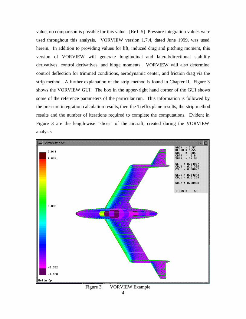
strip method. A further explanation of the strip method is found in Chapter II. Figure 3

shows the VORVIEW GUI. The box in the upper-right hand corner of the GUI shows

some of the reference parameters of the particular run. This information is followed by

the pressure integration calculation results, then the Trefftz-plane results, the strip method

results and the number of iterations required to complete the computations. Evident in

Figure 3 are the length-wise “slices” of the aircraft, created during the VORVIEW

analysis.

Figure 3. VORVIEW Example

5

Aircraft Synthesis (ACSYNT), also developed at NASA Ames, is a conceptual

design code that can perform aerodynamic and performance analysis on an aircraft

configuration based on semi-empirical equations. Three analysis method types are

available: simple analysis, sensitivity and optimization. The simple analysis method will

analyze the design and output the performance details. The sensitivity method is useful

for examining the effect one variable has on another. The optimization method will

minimize or maximize a variable subject to constraints placed on the configuration by the

designer. [Ref. 6] A simple analysis was made on the P 208. ACSYNT enables one to

perform quick trade studies and therefore has tremendous potential use in the conceptual

design stage of an aircraft

.

D. CONFIGURATION THEORY

Recently (1991-2001), extensive work has been done by John Kentfield of the

University of Calgary on what he calls the outboard-horizontal-stabilizer (OHS)

configuration, an example of which is seen in Figure 4. The OHS configuration differs

from the P 208 configuration in that the main wing is unswept and the empennage is

moved aft on wingtip-mounted booms of two to four chord lengths. Kentfield’s

configuration also utilizes vertical stabilizers. Though results obtained for the OHS

configuration cannot be directly compared with the P 208 configuration, the theories

presented would appear largely to apply as the dynamics are similar. Given that no

alternate existing term more adequately describes the P 208’s configuration, the OHS

label will be applied to it. Kentfield states that OHS configurations should employ the

tail as a lifting surface, thereby providing the advantage of a canard configuration. In

fact, the OHS configuration does not have the canard’s disadvantage of requiring the

canard to stall first, thereby reducing the maximum lift capability of the main wing.

Kentfield also suggests that the induced drag of tail lift is somewhat offset by a forward

inclined lift

6

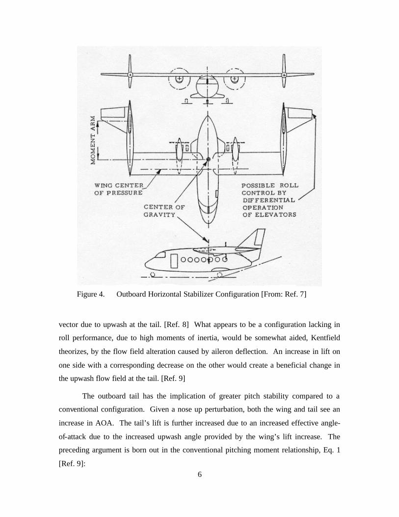
Figure 4. Outboard Horizontal Stabilizer Configuration [From: Ref. 7]

vector due to upwash at the tail. [Ref. 8] What appears to be a configuration lacking in

roll performance, due to high moments of inertia, would be somewhat aided, Kentfield

theorizes, by the flow field alteration caused by aileron deflection. An increase in lift on

one side with a corresponding decrease on the other would create a beneficial change in

the upwash flow field at the tail. [Ref. 9]

The outboard tail has the implication of greater pitch stability compared to a

conventional configuration. Given a nose up perturbation, both the wing and tail see an

increase in AOA. The tail’s lift is further increased due to an increased effective angle-

of-attack due to the increased upwash angle provided by the wing’s lift increase. The

preceding argument is born out in the conventional pitching moment relationship, Eq. 1

[Ref. 9]:

7

1 1mdC dC

d dε

α α = − −

where C1 is a positive constant. A conventional configuration will generally have a

positive value for de/da, due to the immersion of the tail in downwash of the main wing.

An outboard tail configuration will typically have a negative de/da value. Figure 5

shows, for varying wing lift coefficients (CLW), upwash flow angles, eU, vs. displacement

Figure 5. Upwash Flow Angle Over Horizontal Stablizer [From: Ref. 10]

outboard of the wing tip as multiples, n, of the chord of a rectangular planform wing. An

analytical potential flow model of a wing tip vortex far downstream of an aircraft,

specifically Eq. 2, [Ref 10]:

( )22

4 1

41

LW

W

CwU AR Yπ

π

= −

was empirically modified to arrive at Eq. 3 below. Equation 3 describes, in degrees, the

upwash flow in the region from two to four chord lengths downstream of the wing tip.

(1)

(2)

8

[Ref. 10] This equation was used to generate the dotted line in Figure 5. For a complete

discussion of assumptions incorporated the reader is directed to reference 10.

( ) ( )2

3.8711.7667

34 1.0333 13

Un

n

= −

− −

e

p

Kentfield completed direct comparison studies between conventional and OHS

configurations and arrived at the conclusion that an OHS configuration can generate the

same value of CLW as a conventional configuration, with a 15% smaller wing planform

area, largely due to a lifting tail. Additionally, when comparing maximum L/D values,

the OHS configuration’s planform area is an additional 30% smaller than the

conventional configuration. Kentfield also noted that the outboard tailplanes experience

an effective washout due to the decreasing upwash moving outboard of the wingtip as

noted in Figure 5 above.[Ref. 10] It was also determined that increased elevator

effectiveness, due to upwash, resulted in elevator deflections required for level flight of

approximately one-half those required for a conventional aircraft over the lift coefficient

range, 0.2 ≤ CL ≤ 1.2 [Ref. 9]

Scaled Composites, Incorporated built, for NASA, an 18% scale model of a high

altitude research aircraft, the Alliance 1, utilizing the OHS concept, Figure 6. A

Figure 6. Alliance I

(3)

9

VORVIEW analysis was performed on this aircraft by Andrew Hahn, of the NASA Ames

Research Center. [Ref 5] Vortex lattice analysis will yield a known vortex position. This

is an artificial characteristic, but it is sometimes useful. By moving the location of the

tails, it was found that the Alliance 1 configuration was very sensitive to the placement of

these surfaces with respect to the core of the wing tip vortex. The study showed that if

the tails were off by 3.5 degrees (a one foot “miss” in the study cited) from the wingtip

vortex core that the span efficiency dropped by 18%. Such a “miss” of the vortex core

could likely result from the typical movement of the vortex, inboard and down as it

moves aft.

Also stated in reference 5 was the assertion that for the Blohm and Voss design,

with the leading edge of the horizontal tail at the trailing edge of the wing, “…the coring

out of the tip vortex was virtually assured” meaning that no such miss of the vortex by

the horizontal tail will occur.[Ref. 5]

Blohm and Voss anticipated the following benefits from their OHS configuration,

[Refs. 3 and 11]:

- The simplest pusher engine arrangement without the need for a propellor extension shaft, i.e. lightweight, cheap, easy to maintain and reliable.

- Minimum total surface area, combining a short fuselage with small wings and control surfaces, to permit the highest possible maximum speed.

- Lowest overall weight, contingent upon a lighter engine installation, small wings and short fuselage.

- Simplest production, due to constant chord wing and deletion of fin and rudder; load bearing fuselage structure unbroken by integral engine compartment.

- Limited proportion of Duraluminum to overall weight by extensive use of sheet metal in easily manufactured thicknesses.

The previous list is quite interesting for a couple of reasons. First, it is interesting to note

the preoccupation with ease of production and limited use of strategic materials which is

a commentary on the state of Germany in 1944. Secondly, and more interesting,

however, is the absence of any mention of the potential aerodynamic benefits of the

design aside from minimized form drag. This apparent oversight could be explained by a

couple of situations: 1) Blohm and Voss didn’t recognize the aerodynamic benefits,

10

which seems unlikely, or (2) Blohm and Voss didn’t think that the above mentioned

aerodynamic benefits existed. These possibilities seem unlikely since the P 208 is quite a

drastic departure from convention to obtain the benefits listed above. A third possibility

might be that the original reference from which the above list of benefits was taken may

have been part of a proposal to an audience that cared nothing for aerodynamics but was

concerned only about production.

11

II. P 208 COMPUTER MODEL DEVELOPMENT

A. P 208 MODEL DEVELOPMENT

1. Basic P 208 Parameters

Computer model results are, obviously, only as good as the initial data. Gathering

sufficient data to build an accurate model of a German, World War II era, non-production

aircraft presented obvious challenges. A limited amount of original data was available

Figure 7. Example of Primary Blohm and Voss Data [From: Ref. 12]

through the Captured German and Japanese Air Technical Documents holdings of the

National Air and Space Museum Archives Division, [Refs 3 and 12], and through a 1976

German periodical, “Luftfahrt International”, reference 11. Three versions of the P 208

were considered by Blohm and Voss, only the third version with the Daimler-Benz DB

12

603-L engine, the BV P 208.03 is considered in this thesis and, for brevity, will be

referred to as the P 208. One reason the third version was selected was because previous

work had been completed on it at the University of Oklahoma, reference 4. Basic

dimensions were available from primary documents, of which Figure 7 is an example.

References 11 and 12 were used to compile a table of basic data, Table 1. All reference

numbers used with respect to the wing are minus the tails. The 3-view of the P 208,

shown in Figure 1, was scaled using the known data in Table 1 and used to generate data

Table 1. Technical Data Geometry Performance

Wing Area 19.0 m2 Wing Loading (GW) 264 kg/m2

Span 9.58 m Power Loading (GW) 2.4 kg/PS

Aspect Ratio 4.75 Takeoff Power 2100 PS

Span w/tails 12.08 m Climb Power 1800 PS

Length 9.2 m Max Continuous Pwr 1500 PS

Height 3.46 m Reduction Gear 1:1.93

Prop Diameter 3.4 m Time to Max Altitude 27 min

Wing Surface Area 34.4 m2 Takeoff Distance 360 m

Fuselage Area 25.0 m2 Flight Distance (h = 0 km) 1040 km

Tail Boom Area 2 x 2.5 m2 Flight Distance (h = 9 km) 1230 km

Tail Surface Area 6.5 m2 Flight Duration (h = 0 km) 1.79 h

Wing .25c sweep 30o Flight Duration (h = 9 km) 1.85 h

*note, 1 PS = 0.986 HP

for use in the NASA computer codes. This data consisted primarily of body diameters,

fineness ratios, control moment arms and locations for reference points. Because no

anticipated changes to the design were anticipated, all longitudinal measurements were

taken from a zero station defined at the nose of the aircraft. Lateral measurements were

taken from the center line of the fuselage. The degree of accuracy of Figure 1 is

unknown and therefore some uncertainty is introduced in numbers derived from it. The

mean aerodynamic chord (mac) was easily enough determined since the wing is a

constant chord of 2 meters (6.56 ft); the mac was then located at the geometric center of

the wing, i.e., b/4. The only data available on the airfoil was that it was 12½ % thick.

[Ref. 11] It is highly likely that the particular airfoil used was a Blohm and Voss

13

proprietary airfoil. A NACA 23012 airfoil was chosen for analysis since it is

representative of the technology of the times and has good performance. No wing twist

was used and an angle of incidence of two degrees was taken from reference 4. For the

tail surfaces a NACA 0010 at minus three and a half degrees of incidence was used in

accordance with reference 4. RAM has the capability to accept an airfoil coordinate file

and apply it to the geometry of the aircraft under consideration. Lacking any information

on location of the center of gravity (CG) of the aircraft, an estimate was made using the

tip-back angle. Raymer states that the most aft CG location should be forward of a line

that is defined by a 15 degree angle forward of a vertical line at the point where the main

gear touch the ground. [Ref. 13] Using this methodology the P 208’s CG was placed at

Figure 8. Engine Power vs. Altitude [From: Ref. 12]

32% mac. VORVIEW calculated the aerodynamic center (AC) of the aircraft to be at

50% mac. Sufficient engine data was available from Table 1 and Figure 8 to model the

power plant in ACSYNT. Moments of inertia were estimated using the weight values

14

given in the table in Appendix A and approximating their point mass location. These

estimates were within 10% of those given in reference 4 and so the values of reference 4

were used as shown in Table 2.

Table 2. Moments of Inertia (slug ft2)

IXX = 18,143 IYY = 12,370

IZZ = 28,474 IXZ = 200

Determining a configuration’s zero lift drag coefficient (CDo) is a significant task

since it is a major factor in determining the aircraft’s performance. Primary data on a CDo

build-up was available as shown in Figure 9, and resulted in a CDo equal to 0.0201.

Reference 4 also performed a component build-up for CDo determination resulting in a

Figure 9. Drag Polar Build Up [From: Ref. 12]

15

significantly lower value of 0.0152. Unfortunately, the Reynolds number at which each

of the aforementioned CDo values was determined is unknown. ACSYNT also performs a

component build up, based on geometry inputs, and estimated a CDo at each flight

condition analyzed. For the P 208, ACSYNT estimated a CDo of 0.0166 in the cruise

condition. Though it is an inviscid code, VORVIEW has the capability to estimate

friction drag. The term ‘friction drag’ is used, as opposed to, CDo because the

VORVIEW values are not restricted to the zero lift condition. VORVIEW can accept

drag polar data files for specified Reynolds numbers. As the aircraft’s planform is

‘sliced’ chordwise the drag polar corresponding to the local characteristic length is

applied to the slice. Due to the difficulty of obtaining drag polars for input, only a

cursory look at this feature of VORVIEW was taken. Drag polars, provided by Andrew

Hahn of NASA Ames Research Center, using MSES polar driver version 3.0, were

entered for a NACA 0010 airfoil at Re = 3.85106 corresponding to the tail, a NACA

23012 airfoil at Re = 13.8x106 corresponding to the wing and a fuselage- like shape at Re

= 55.5x106. These Reynolds numbers correspond to a mid-envelope flight condition of

21,000 feet and a flight Mach number of M = 0.55. The use of these three sectional drag

polars resulted in an average friction drag estimate of 0.0199 that varied from a low value

of 0.00958 at 2 degrees AOA to a high value of 0.048 at 15 degrees AOA.

EXCEL was used to program the USAF DATCOM equations for the P 208

component drag build up. The spreadsheet allows the computation of the P 208 CDo

under any given flight condition, with the local Reynolds Number for each component

calculated for the given condition. For a cruise condition of 29,500 ft at Ma = 0.57, a CDo

= 0.0168 was calculated via this method; for the flight condition used for the VORVIEW

analysis (above) CDo = 0.162.

Figure 10 illustrates the dependence of the CDo for the XP-41 on seemingly small

factors. Because of this small factor dependence, and the fact that Blohm and Voss had

more detailed information on the aircraft and likely expended more effort than anyone

else, the Blohm and Voss value of CDo was used in this current analysis of the P 208,

despite the lack of Reynolds number information on which it was based. A non-varying

CDo should be accurate for a first order linear analysis.

16

The previous discussion of CDo should cast doubt on any attempt to directly

compare various aircraft CDo values of unknown origin as a means of determining any

relative aerodynamic benefits of a given configuration. For example it would be folly to

attempt to compare the P 208’s CDo, using any of the methods above, to that of the P-51

Figure 10. Drag Study on the XP-41 [From: Ref. 15]

Mustang which reference 15, using none of the above methods, has as 0.0161.

Furthermore, though it may be tempting to compare a unique configuration such as the P

208s against a very conventional configuration such as the P-51, Figure 10 indicates that

any proposed configuration advantage/disadvantage may be masked by other factors. For

example, the boundary layer diverter, on the radiator intake, that is widely accepted as a

key feature leading to the P-51’s outstanding performance, is not evident on the P 208;

this one feature could mask any potential drag reduction of the OHS configuration.

Though it looks like the P 208 should have a form drag advantage given the shortened

fuselage and small vee-tail, a proper comparison would require developing a simple OHS

model and a conventional configuration, with the wing parameters and tail volume

coefficients held constant, and analyzing each with the same method. Such an analysis

was not performed for this thesis.

17

2. Flight Conditions

Four flight conditions were chosen for performance and stability and control

analysis, in accordance with reference 15. These flight conditions, summarized in Table

3, should adequa tely cover the flight envelope shown in Figure 11. Flight condition lift

coefficients are based on unaccelerated flight at a weight of 10,300 pounds,

corresponding to the weight on which the flight envelope was developed. Figure 11

depicts a clean (i.e. flaps and landing gear retracted), unaccelerated flight envelope and

therefore the Approach configuration is not depicted. The sea level penetration condition

is maximum velocity at sea level.

Table 3. Flight Conditions Flight Condition Altitude M CL

1 Approach (40o flaps) 0 0.17 1.2

2 Sea Level Penetration 0 0.52 0.125

3 Cruise 29,500 ft (9 km) 0.57 0.344

4 Maximum Velocity (Vmax) 31,000 ft (9.5 km) 0.73 0.225

Figure 11. P 208 1 G Performance Envelope [After: Ref. 12]

18

THIS PAGE INTENTIONALLY LEFT BLANK

19

III. P208 PERFORMANCE

A significant volume of German performance estimates for the P 208 is available

for numerous altitudes and power settings, reference 3. However, its interpretation was

beyond the author’s capability. The interpretation was not merely a matter of language

but variable definition. An example of the data available is included as Appendix B.

The primary analysis tool used to examine the performance of the P 208 was

VORVIEW. Example VORVIEW summary output and stability and control derivative

output files are included as Appendix C. As previously mentioned, VORVIEW is an

inviscid code that uses a Trefftz-plane analysis as a check to the pressure integration

method. VORVIEW computes both pressure integration and Trefftz-plane values for

CDi/CL2; these values where checked for agreement. When a disagreement occurred in

the CDi/CL2 values, it was always due to a pressure integration value that was too

optimistic, often resulting in span efficiency factors greater than one. To remedy this

situation, the leading edge suction/vortex lift multiplier (SPC), in the VORVIEW initial

conditions file, was varied by iteration until agreement was reached between the two

analyses.

The SPC variable is used to account for the presence of vortex lift using the

Polhamus suction analogy and was therefore typically quite low for the P 208, about 0.2

for the cruise condition. The Polhamus suction analogy states that the extra normal force

that is produced by a leading edge vortex on a highly swept wing at high angles of attack

is equal to the loss of leading edge suction associated with the separated flow.

VORVIEW provides a value of span efficiency for every flight condition

analyzed. Span efficiency as a function of CL is shown in Figure 12. The large variation

that occurs at low values of AOA is not unexpected as span efficiency is sensitive to CL.

The large negative AOAs, thought impractical, are included to show that the curve will

tend to smooth out at larger absolute values of CL. Figure 12 shows an average span

efficiency of about 61% with a peak of 71% at lift coefficients corresponding to high

airspeeds. A drag polar, for an unknown flight condition, is available from primary

German data: CD = 0.0201+0.0960CL2. A value of span efficiency, e, can be backed out

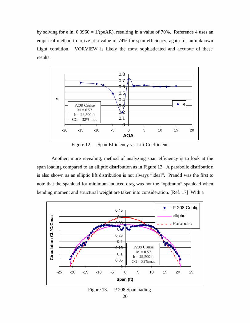
20

by solving for e in, 0.0960 = 1/(peAR), resulting in a value of 70%. Reference 4 uses an

empirical method to arrive at a value of 74% for span efficiency, again for an unknown

flight condition. VORVIEW is likely the most sophisticated and accurate of these

results.

00.10.20.30.40.50.60.70.8

-20 -15 -10 -5 0 5 10 15 20

AOA

e

e

Figure 12. Span Efficiency vs. Lift Coefficient

Another, more revealing, method of analyzing span efficiency is to look at the

span loading compared to an elliptic distribution as in Figure 13. A parabolic distribution

is also shown as an elliptic lift distribution is not always “ideal”. Prandtl was the first to

note that the spanload for minimum induced drag was not the “optimum” spanload when

bending moment and structural weight are taken into consideration. [Ref. 17] With a

0

0.05

0.1

0.15

0.2

0.25

0.3

0.35

0.4

0.45

-25 -20 -15 -10 -5 0 5 10 15 20 25

Span (ft)

Cir

cula

tio

n C

L*C

/Cm

ac

P 208 Config

elliptic

Parabolic

Figure 13. P 208 Spanloading

P208 Cruise M = 0.57

h = 29,500 ft CG = 32% mac

P208 Cruise M = 0.57

h = 29,500 ft CG = 32%mac

21

configuration like the P 208, it is likely that a more parabolic lift distribution would be

desirable for structural reasons. Figure 13 shows that the P 208 lift distribution falls

somewhere between the elliptic and parabolic ideals. The tail booms are at 15 ft. with the

tails outboard of the booms. It should be noted that in the cruise condition, as shown in

Figure 13, that the tails are in fact lifting surfaces.

Figure 14 show a comparative lift distribution with and without aileron deflection.

This condition was examined to evaluate Kentfield’s theory that the OHS configuration

can aerodynamically offset some of the configuration’s roll performance penalty due to

its high moments of inertia. Figure 14 clearly shows that the increased lift due to a

negative aileron deflection (down) results in increased lift on the adjacent tail, as

predicted by Kentfield. The increased lift on the tail is due to the strengthened wing-tip

vortex caused by the local lift increase resulting from the aileron deflection. For a

positive aileron deflection (up) the opposite is true and lift is reduced. The coupling

effect seen should assist the aircraft in its roll performance.

-0.1

0

0.1

0.2

0.3

0.4

0.5

0.6

-25 -20 -15 -10 -5 0 5 10 15 20 25

Span (ft)

Cl

15 deg ail defl

0 ail defl

Figure 14. Spanloading with Aileron Deflection

The lift curve for the aircraft at Mach 0.57 is shown in Figure 15. Because it is an

inviscid code, VORVIEW will not predict stall for the aircraft. The figure shows that the

zero lift AOA for the aircraft is –2.7 degrees and that CLα = 0.0824. Additionally, the

zero AOA CL = 0.216 which roughly corresponds to the Vmax flight condition. This could

P208 M = 0.57 h = 29,500 ft CG = 32%mac

22

mean that Blohm and Voss optimized the aircraft for top speed or that the angle of

incidence of the main wing or the airfoil section chosen for this analysis was incorrect.

With the previous discussion of CDo, it would seem inevitable that drag polars

from various sources or methods would differ somewhat. Four drag polars are shown in

Figure 16. The first polar (square symbols) is VORVIEW generated with both form drag

and span efficiency varying for each data point. The second polar (diamond symbols) is

y = 0.0824x + 0.2156

-0.25

0

0.25

0.5

0.75

1

1.25

1.5

1.75

-7 -5 -3 -1 1 3 5 7 9 11 13 15 17

AOA (deg)

CL

CL

Linear (CL)

Figure 15. P 208 Lift Curve

the Blohm and Voss drag polar. The third polar (triangle symbols) was generated by

Tipton: CD=0.0152+0.906CL2. [Ref. 4] The last polar (X symbols) represents a

combination of a DATCOM CDo with VORVIEW CDis. The first polar shows a large

variation in friction drag, explained in the previous discussion in Chapter II. While this

variation is more realistic than a non-varying CDo, the magnitude of the change is

P208 M = 0.57

h = 29,500 ft CG = 32%mac

23

-0.5

-0.25

0

0.25

0.5

0.75

1

1.25

1.5

1.75

0 0.05 0.1 0.15 0.2 0.25 0.3

CD

CL

VORVIEWBlohm and VossTiptonDATCOM + Vorv

Figure 16. Drag Polar Comparison

questionable. The fourth polar provides for the greatest flexibility; a CDo for any given

flight condition can be used and CDi variations can be captured with VORVIEW.

In all likelihood, the most accurate drag polar for the P 208 is one that

incorporates the most accurate, Blohm and Voss derived, CDo with the CDis from

VORVIEW. This polar is plotted against the Blohm and Voss polar in Figure 17.

VORVIEW CDi values are probably the most accurate because they are calculated at each

flight condition and do not rely on a non-varying value of CDi/CL2.

-0.4

-0.2

0

0.2

0.4

0.6

0.8

1

1.2

1.4

1.6

0 0.05 0.1 0.15 0.2 0.25 0.3

CD

CL

Blohm and Voss

BV + VORVIEW

Figure 17. P 208 Drag Polar

24

Lift over drag ratios are given, in Table 4,for each flight condition using each of

the drag polars in Figure 17. For the approach condition, a CDo = 0.18 from reference 4

was used to account for landing gear and flaps. A comparison of the results in Table 4

generally shows agreement within 5%. The composite polar resulted in the more

conservative estimate.

Table 4. P 208 L/D Approach SL Penetration Cruise Max Velocity

Blohm and Voss 3.8 5.8 10.9 9.0

BV + VORVIEW 3.5 5.6 10.6 8.8

25

IV. STABILITY AND CONTROL

A. ELEVATOR TRIM

With the CG at 32% mac and the neutral point at 50% mac, the P 208 has a rather

large static margin (SM) of 18%. In the approach condition, strong wing tip vortices will

be present due to high lift generation. This condition makes the tail surfaces effective at

generating lift, but hinders their ability to counter the nose-down pitching moment due to

the flaps. The above condition results in a large elevator deflection (δe) required to trim

the approach condition, see Table 5. Because this is such a critical phase of flight, a few

scenarios were examined to address the large control deflection requirement. A full-span

flap configuration was also considered. It has been suggested that due to the increased

effectiveness of the ailerons, or by using the outboard surfaces for roll control, larger or

even full-span flaps could be utilized by the OHS configuration. Table 5 is a summary of

Table 5. Approach Configuration Trim Condition Configuration CG/SM AOA δe

1 Standard (70% Span Flaps) 32%mac/18% 1.42o -19.8o

2 Full-Span Flaps 32%mac/18% -1.17o -47.1o

3 All Moving Tail 32%mac/18% 1.23o -17.0o

4 Reduced Static Margin 40%mac/10% 0.61o -9.3o

5 Reduced Flaps (40% Span) 32%mac/18% 4.11o -7.7o

Trimmed for CL=1.2, 40o flap deflection

five conditions examined for an approach condition of Ma = 0.17 and a flap deflection, dF

= 40o. Control surface deflections and AOAs were determined by VORVIEW. The first

condition is for the standard configuration. Condition 1 assumed a flap size of 70% span

(excluding the fuselage area) and an elevator surface of 30% of the chord of the

stabilizer. Condition 1 resulted in a rather large control deflection of almost 20 degrees.

Condition 2 looked at a configuration using full-span flaps. For the given static margin it

is obvious that full-span flaps are not an option as the control deflection shown would

result in control surface stall. Condition 3 was added to examine any increase in control

power of an all-moving tail. An all-moving control surface does not appear to provide

26

the requisite control force at an acceptable deflection. Condition 4 looked at a reduced

static margin. Reducing the static margin to 10% by moving the CG back to 40% mac

resulted in an acceptable control deflection. The feasibility of the CG shift or its affect

on stability and control was not considered by the author. Condition 5 looked at the

result of reducing the flap span. The flaps were reduce to 40% span. Because the wings

are swept, reducing the span of the flaps brings their center of pressure inboard and

forward. This movement of the center of pressure reduces the nose down pitching

moment created by the flaps and results in the lowest required control deflection to trim

the approach configuration.

Trim conditions for the four flight conditions, defined in Chapter II, are shown in

Table 6. The fact that the cruise condition control deflection for trim is negligible

suggests that the assumed angle of incidence for the tail of –3.5o is probably correct.

Table 6. Trimmed Conditions Flight Condition CG/SM AOA δe

Approach 0.32c/18% 1.42o -19.8o

Sea Level Penetration 0.32c/18% -0.6o 3.27o

Cruise 0.32c/18% 1.55o 0.04o

Maximum Velocity 0.32c/18% -0.08o 2.15o

B. LONGITUDINAL STABILITY

The coordinate sign convention utilized for the trim and stability and control

analysis is that shown in Figure 18.

A casual observation of the P208 may lead one to believe that the tails surfaces

are too small. An examination of tail volume coefficients will support this observation.

Dividing the P 208’s vee-tail into projected vertical and horizontal areas allows an

analysis of the tail volume coefficients. Using these areas as given in reference 4, the

horizontal tail volume coefficient (CHT) was found to be CHT = 0.326. With a 5%

reduction in required CHT that Raymer suggests for a T-tail, due to the clean air seen by

the horizontal, and a further arbitrary 5% reduction due to the proposed increased

dynamic pressure from the wing tip vortex, a typical value of CHT for this application

27

should be about CHT = 0.45. [Ref. 14] This comparison suggests that the horizontal tail

is approximately 28% too small.

Figure 18. Coordinate Sign Convention [From: Ref. 17]

y = -0.0162x + 0.0225

-0.25

-0.2

-0.15

-0.1

-0.05

0

0.05

0 3 6 9 12 15 18

AOA (deg)

CM

cg

Figure 19. Static Stability

P208 M = 0.57

h = 29,500 ft CG = 32%mac

CM = 0.0225 – 0.0162a

28

Utilizing CM values determined by VORVIEW, an initial look at static stability

shows that, for the given flight conditions, the aircraft is longitudinally statically stable,

that is its initial tendency upon being disturbed will be to return to its equilibrium

position. This result was not surprising given the large static margin. Figure 19 shows

that both criteria necessary for longitudinal static stability exist, namely that CM0 is

positive, CM0 = 0.0225, and the slope of the curve is negative, CMa = -0.0162 per degree.

VORVIEW is an excellent tool for examining an aircraft’s dynamic stability. The

code will perturb the aircraft’s initial conditions by one degree around each axis to

determine dimensionless stability derivatives. Dimensionless derivatives were

determined for a trimmed aircraft in each of the following flight conditions: Approach,

Sea Level Penetration, Cruise and Maximum Velocity, as defined in Chapter II. The

dimensionless derivatives were dimensionalized as shown in Appendix D and are given

in the Appendix. The equations of motion, which have been linearized as described by

Schmidt [Ref. 18], were grouped into longitudinal and lateral-directional and considered

separately in the governing state space equation, { } [ ]{ } { }x A x B δ= +& . The longitudinal

plant matrix, [A], state vector, {x}, and control matrix, {B} are shown below in equations

4, 5 and 6 respectively.

[ ]

( )( ) ( )

( )( ) ( )

( ) ( )( )

( )

0

0

0 cos

sin

0

0 0 0 1

U

qU

q qU U

X gX U U

V ZUZ Z gU Z U Z U Z U ZA

M M U ZUM MUZ M M ZU Z U Z U Z

α

α

α α α α

αα α α α

α α α

− Θ

+ − Θ − − − −= + ++ + − − −

& & & &

&& &

& & &

{ } ( ) ( ) 0T

X Z M M ZB U U Z U Zδ δ δ α δ

α α

+= − − &

& &

{ } [ ]/T

x u U qα θ=

(4)

(5)

(6)

29

An aircraft’s linearized longitudinal dynamics will normally consist of two pairs of

complex conjugate roots corresponding to the short-period and long-period or phugoid

modes. The real part of the root will indicate the modal damping, a negative value

corresponds to positive damping. The imaginary part of the root is the mode’s damped

natural frequency. The state equation was coded in MATLAB; a code listing is given in

Appendix E. Solving the corresponding longitudinal eigenvalue problem results in the

information about the longitudinal dynamics of the system found in Table 7.

Table 7. Longitudinal Roots Approach SL Penetration Cruise Max Velocity

Short- Roots (λ) -0.7025 ± 1.789i -2.5182 ± 6.284i -0.9644 ± 3.9415i -1.2422 ± 5.1247i

Period ωn (rad/sec) 1.9223 6.7694 4.0578 5.2731

ζ 0.3654 0.372 0.2377 0.2356

Long- Roots (λ) -0.0200 ± 0.2248i -0.0204 ± 0.0708 -0.0365 ± 0.0713i -0.0107 ± 0.0601i

Period ωn (rad/sec) 0.2257 0.0737 0.0801 0.061

ζ 0.0884 0.2768 0.0455 0.175

The MATLAB code allows one to excite a stability mode with its eigenvector, via the

initial command, and for exciting the system with a simulated control input, via the step

command. Although the aircraft’s plant matrix contains information on all modes, the

use of an initial condition corresponding to a mode’s eigenvector will assure only that

mode will respond. [Ref. 18]

The short-period roots for the cruise condition show the mode is positively

damped. Likewise, Figure 20 shows that, in the cruise condition, the short period is

stable and damped, evident from the decay of the oscillations. The eigenvector

normalized to alpha gives clarifying information to the figure, namely it shows: that the

velocity perturbation (u/U) is small, about 1.7% of the trim speed, pitch angle (θ) is close

to the angle-of-attack (α) in magnitude (98.4%) and phase (lags by 12.6°), pitch rate (q)

leads α by 91° and that q leads the θ by 103.5° all of which are normal short-period

behavior. [Ref. 18] Each flight condition examined showed normal short-period behavior

with the cruise and Vmax conditions being relatively lightly damped.

30

Figure 20. Short-Period Response to Initial Condition

0.0170 66.51

3.992 90.90.984 12.6

uU

qα

θ

= −

o

o

o

R

RR

Figure 21 shows the long-period response to eigenvector excitation. The

eigenvector, normalized to the velocity perturbation, is shown as equation 8 for

amplification. In the cruise condition, the P208, demonstrates a typical long-period

response. Light damping is evident with a 78 second period and a slow decay of the

oscillation amplitude. Comparatively, the damping ratio, ?, for the long-period is an

order of magnitude smaller than that for the short period, Table 7. Also typical of the

long-period is that the α component of the eigenvector is much smaller than the u/U

component, opposite of the short period. Again it is seen that the rate term, q, leads

P208 Cruise M = 0.57

h = 29,500 ft CG = 32%mac

(7)

31

Figure 21. Long-Period Response to Initial Condition

10.0168 178.40.1140 0.91.400 96.0

uU

qα

θ

−

= −

−

o

o

o

RR

R

)

displacement term, θ, by 95° in this case. The P208 exhibited normal long-period

behavior for the four flight conditions examined.

The complete system response for the P208, due to an elevator control step input,

can be seen in Figure 22. For the given flight condition, the P208 exhibits a typical

system response to the given input. Figure 22 shows that the short-period motion,

characterized by a, is mostly damped by 5 seconds while the long-period motion,

characterized by u/U, will continue to oscillate for a few minutes. A positive elevator

step control input will result in a nose-down pitch attitude, after the short-period damps

out, the long-period exhibits normal features. The α component maintains a nearly

P208 Cruise M = 0.57

h = 29,500 ft CG = 32%mac

(8)

32

constant negative value. Pitch rate, q, will oscillate and finally reach a zero value. Pitch

angle, θ, will oscillate and finally reach a constant slightly negative value. The u/U

component will oscillate and eventually reach a positive steady value. The P 208

exhibited typical longitudinal behavior to a step input for all flight conditions examined.

[Ref. 18]

Figure 22. Longitudinal Response to Elevator Step Input

C. LATERAL-DIRECTIONAL STABILITY

Again using areas from reference 4, the vertical tail volume coefficient (CVT) was

found to be CVT = 0.0248. Looking to Raymer [Ref. 14] once again for a representative

CVT and subtracting a nominal 5% for increased dynamic pressure due to the wing tip

vortices results in a desired CVT value of about 0.05. [Ref. 14] Thus, it appears that the

vertical surface is prehaps 50% too small. This can indicate a directional stability

problem with the design. Lateral stability increases with both wing sweep and dihedral.

P208 Cruise M = 0.57

h = 29,500 ft CG = 32%mac

33

Thus, with 30 degrees of sweep and six degrees of dihedral the design should be laterally

stable.

VORVIEW and MATLAB, with the linearized equations of motion, were used to

examine the P208’s lateral-directional dynamic stability. Lateral-directional dimensional

stability derivative values, computed from VORVIEW dimensionless derivatives, are

given in Appendix D. The lateral-directional plant matrix, control vector (applied for

rudder or aileron deflection as required) and state vector used in the governing state space

equation are given below as equations 9, 10 and 11 respectively, with short-hand notation

equations 12 – 14.

[ ]( ) ( )

{ } { }{ } { }

( )( )

( )2

0

'

'

1( )1

cos

' ' 0 '0 0 0 1' ' 0 '

' 0 '

:

xzn n n

x

xzn n n

x

xz

x z

p r

p r

p r

T

T

IL G L NI

IN G N L I

GI

I I

Y Y Y UgU U U U

L L LA

N N N

YB L NU

x p r

where

β

β

β

δδ δ

β φ

= +

= +

=−

−Θ

=

=

=

Solving the eigenvalue problem for the lateral-directional (4x4) plant will normally give a

complex conjugate pair of roots that describe the Dutch-roll and two real roots; the faster

of the real roots describes the roll response and the slower one describes the spiral. [Ref.

18] Table 8 gives the results of solving the eigenvalue problem for the lateral-directional

plant matrix. It should be noted that only the sea level penetration condition has a

complex conjugate pair of roots with a negative real part, thus only this condition is

(9)

(10)

(11)

(12)

(13)

(14)

34

Table 8. Lateral-Directiona l Roots

Approach SL Penetration Cruise Max Velocity

Dutch- Roots (λ) 0.2196 ± 1.075i -0.1537 ± 0.4126i 0.0093 ± 1.252i 0.0190 ± 0.7750i

Roll ωn (rad/sec) 1.0980 0.4403 1.2520 0.7752

ζ -0.2001 0.3491 -0.0075 -0.0245

Roll Roots (λ) -1.6040 -3.5549 -1.5390 -1.8732

ωn (rad/sec) 1.6040 3.5549 1.5390 1.8732

ζ 1.0000 1.0000 1.0000 1.0000

Spiral Roots (λ) -0.0412 -0.0242 -0.0110 -0.0154

ωn (rad/sec) 0.0412 0.0242 0.0110 0.0154

ζ 1.0000 1.0000 1.0000 1.0000

damped. Both the roll and spiral modes exhibit negative real roots, indicating that these

modes are non-oscillatory and convergent.

Once again, for each of the four flight conditions, each lateral-directional mode

was excited by its eigenvector. Figure 23 shows the Dutch-roll response to excitation by

the eigenvector normalized to the sideslip angle, β . Although yaw angle (ψ) is not an

eigenvector component, and not shown in Figure 22, it is useful when examining the

Dutch-roll mode shape. For a typical Dutch-roll, the magnitudes of ψ and β will be

nearly equal while their phase angles will be about 180 degrees out of phase. This

relationship gives an aircraft’s c.g. a nearly straight trajectory during a Dutch-roll

oscillation, when viewed from overhead. [Ref. 18] The yaw angle perturbation was

estimated by, ˆ1;i

n

e where rφψ ψ ψω

−= & & ; , resulting in 0.93 93.2ψ = R . Figure 23 and the

Dutch-roll eigenvalue roots show that the Dutch-roll mode is undamped and slightly

35

Figure 23. Dutch-Roll Response to Initial Condition

12.550 137.02.037 47.51.664 268.4

p

r

β

φ

− = − −

RR

R

unstable for the cruise condition of flight. As expected, only the sea- level penetration

condition exhibited a stable Dutch-roll mode.

Figure 24 shows the roll response, as excited by the eigenvector normalized to p.

The roll mode is, characteristically, dominated by roll angle, φ, and roll rate, p, with small

β and yaw rate, r, components. All flight conditions exhibited similar roll characteristics.

P208 Cruise M = 0.57

h = 29,500 ft CG = 32%mac

(15)

36

Figure 24. Roll mode Response to Initial Condition

0.04471

0.64980.0282

p

r

β

φ

=

Figure 25 shows the spiral mode as excited by the eigenvector normalized to φ.

The cruise condition spiral shown is stable and is typical of all flight conditions

examined. The spiral mode is, characteristically, dominated by the roll angle component,

φ. [Ref. 18]

P208 Cruise M = 0.57

h = 29,500 ft CG = 32%mac

(16)

37

Figure 25. Spiral mode Response to Initial Condition

0.00310.0108

10.0564

p

r

β

φ

=

D. FLYING QUALITIES

Using the previous stability and control data, the P 208’s flying qualities were

assessed in accordance with MIL-F-8785C, (Military Specification Flying Qualities of

Piloted Airplanes). Each of the four flight conditions were assessed in the trimmed,

stick-fixed mode. The P 208 was evaluated as a Class IV aircraft, that is, a high

maneuverability aircraft. The three flight phase categories and three levels of flying

qualities from MIL-F-8785C are discussed below. [Ref. 18]

P208 Cruise M = 0.57

h = 29,500 ft CG = 32%mac

(17)

38

Flight Phase Categories-

A. Non-terminal Flight Phases that require rapid maneuvering, precision tracking, or precise flight-path control, i.e., air-to-air combat, ground attack, terrain following, ect.

B. Non-terminal Flight Phases that are normally accomplished using gradual maneuvers and without precision tracking, i.e., climb, cruise, loiter, ect.

C. Terminal Flight Phases normally accomplished using gradual maneuvers and usually require accurate flight-path control, i.e., takeoff, approach, landing, ect.

Levels of Flying Qualities-

1. Flying qualities clearly adequate for the mission Flight Phase.

2. Flying qualities adequate to accomplish the mission Flight Phase, but some increase in pilot workload or degradation in mission effectiveness, or both exists.

3. Flying qualities such that the airplane can be controlled safely, but pilot workload is excessive or mission effectiveness is inadequate, or both.

For the short-period motion, the P 208 has Level 1 flying qualities for category C

Flight Phases and for category A at low altitude and high airspeed. At higher altitudes

the short-period drops to Level 2 for category B Flight Phases and Level 3 for category

A. The P 208’s long-period is Level 1 across the board. The P 208 has unacceptable

flying qualities in the Dutch-roll mode, except at low altitudes and high airspeeds where

it exhibits Level 1 qualities for Flight Phases A and B, except for air-to-air combat and

ground attack where it is Level 2. The P 208 is Level 1, for all flight conditions

examined, in roll and spiral performance.

39

V. CONCLUSIONS AND RECCOMENDATIONS

A. CONCLUSIONS

1. Configuration Suitability

It is, of course, the configuration and its applicability to future designs, and not

the P 208 itself that is of primary interest. Some of Kentfield’s conclusions on the OHS

configuration have been observed in the analysis of the P 208. The tails are, in fact,

lifting surfaces for most phases of flight, and therefore his claims of reduced main wing

planform area versus a conventional configuration appear valid. Roll performance is

adequate, as seen by the P 208’s Level 1 roll performance. Again, Figure 14 appears to

verify Kentfield’s theory on increased roll performance as stated in Chapter I. Greater

pitch stability, as theorized by Kentfield, did not materialize as the P 208 had Level 2 and

3 short period flying qualities at higher altitudes and airspeeds. This is likely due to the

low lift coefficients and corresponding low circulations and weak wing tip vortices

occurring at the cruise and Vmax conditions in addition to the short coupling and small tail

size of the P 208. Pitch control presented a problem in the approach configuration for the

P 208 as analyzed herein. Reducing the static margin corrected the problem but no effort

was made to examine how this would further affect stability and control, which may pose

a problem since already small tail volume coefficients would be further reduced by an aft

movement of the CG. Stability and control should present no major difficulties, even

with the small tails, but require a pitch and a yaw damper at a minimum to bring the

short-period and Dutch-roll up to Level 1. As far as performance is concerned, Blohm

and Voss predicted a lower weight and surface area due to small wings, control surfaces

and fuselage. Nothing in the analysis would appear to contradict these predictions.

2. NASA codes

RAM was an excellent tool for the analysis of the P 208. The code lends itself

well to quick building and adjusting of concepts, though adding fine nuances, such as

complex body shapes, requires much more skill and time. Despite its lack of

documentation the code is quickly learned by sitting down and using it. For

40

reproducibility in future studies, a copy of the P 208 RAM input file is included as

Appendix F.

VORVIEW allows for a very quick examination of a proposed configuration

developed in RAM. The inputs to and execution of VORVIEW require a fraction of the

time necessary to produce the same results by empirical methods. Unfortunately, a true

evaluation of VORVIEW’s accuracy in predicting an unconventional configuration’s

performance was not possible. Insufficient Blohm and Voss data was available to make

such an evaluation. Also lacking any flight data or wind tunnel data it would be unwise

to evaluate a modern design code against 1940s prediction methods. Some comparisons

are, however, available. Span efficiency, as predicted by VORVIEW was apparently

13% lower than the German value and 18% lower than the value given in reference 4.

Reference 4 also presented non-dimensional stability derivatives, derived using Roskam,

reference 15, and longitudinal and lateral-directional roots for two flight conditions.

Damping ratios and natural frequencies were calculated from the roots given and

compared to those obtained from VORVIEW derivatives. Considering the fact that the

flight conditions in reference 4 were no further defined than “Powered Approach” and

“High-Speed Cruise” at a static margin of 5%, the agreement of the longitudinal

characteristics was exceptional. All values of damping ratio and natural frequency for the

longitudinal modes agreed within 28% except for long-period damping in the approach

configuration which was 2.6 times greater in reference 4. Conversely, there was no

agreement for the lateral-directional modes. VORVIEW showed an unstable Dutch-roll

mode where reference 4 was stable, a stable spiral mode where reference 4 showed the

mode as unstable and roll roots that were three times greater than found in reference 4.

Unfortunately no useful conclusions can be drawn from these comparisons since no

“correct” answer is available.

ACSYNT is a powerful tool. However, its utility was not ideally suited to the

problem at hand. ACSYNT is not so much an analysis as it is a development tool.

Through its sensitivity and optimization routines ACSYNT can quickly apply empirical

equations drastically reducing man-hours required to perform trade studies. A working

ACSYNT file for the P 208 has been created, Appendix G, and preliminary convergence

to VORVIEW performance numbers completed. ACSYNT should be further used to

41

optimize the configuration for various defined missions. The requirements for its

products occur early in the design process, before someone could learn the code and

become proficient at its use.

The common weakness among the NASA codes, as far as their utilization

at NPS is concerned, was the reliance on support from NASA personnel for their

utilization. The minimal documentation, for RAM and VORVIEW, was the cause of

much of this reliance.

B. RECCOMMENDATIONS

1. If more than an academic interest exists in the OHS configuration, the next course

of action should be a detailed structural analysis to determine if any structural

penalties of the configuration will outweigh its benefits.

2. With a wind-tunnel model now available, experiments should be conducted to

determine the accuracy of VORVIEW in the analysis of the configuration; thus

giving a confidence level to any VORVIEW analysis of similar designs.

3. The P 208 ACSYNT model should be refined, and sensitivity and optimization

analysis run to improve the configuration.

4. A direct RAM/VORVIEW comparison should be completed of a conventional

and OHS configuration with wing planforms and tail volume coefficients held

constant.

5. A radar cross-section analysis should be performed to determine the

configuration’s potential benefits in this area.

42

THIS PAGE INTENTIONALLY LEFT BLANK

43

LIST OF REFERENCES

1. Cowin, Hugh W., “Blohm und Voss Projects of World War II,” Air Pictorial, pp. 312- 316, October, 1963.

2. Schick, Walter and Ingolf Meyer, Luftwaffe Secret Projects: Fighters 1939-1945, World Print Limited, Hong Kong, 1997.

3. Blohm & Voss “Performance data for various Blohm und Voss fighter airplanes,” National Air and Space Museum, German/Japanese Captured Air Technical Documents Microfilms Hamburg, Germany, May-December 1944.

4. Tipton, Brian, “The Preliminary Design Analysis of a Unique Semi-tailless Aircraft Configuration,” Masters Thesis, University of Oklahoma, Norman, OK, 1995.

5. Hahn, Andrew, “An Independent Assessment of Scaled Composites Incorporated’s Model M287-9 (Alliance 1) Inviscid Aerodynamics Using a Vortex Lattice Code,” NASA Ames Research Center, November 16, 1998.

6. “User Guide to Acsynt and Create,” Naval Postgraduate School, Monterey, CA, No Date.

7. Kentfield, John, “Aircraft Configurations with Outboard Horizontal Stabilizers,” Journal of Aircraft, vol. 28, no. 10, pp. 670-672, October, 1991.

8. Kentfield, John, “Case for Aircraft with Outboard horizontal Stabilizers,” Journal of Aircraft, vol. 32, no. 2, pp. 398-403, March-April 1995.

9. Kentfield, John, “The Aspect-Ratio Equivalence of Conventional Aircraft with Configurations Featuring Outboard Horizontal Stabilizers,” Paper 975591, 1997 SAE/AIAA World Aviation Congress, October 13-16, 1997.

10. Kentfield, John, “Influence of Aspect Ratio on the Performance of Outboard Horizontal-Stabilizer Aircraft,” Journal of Aircraft, vol. 37, no. 1, pp. 62-67, January-February 2000.

11. “Blohm & Voss P 208,” Luftfahrt International, vol. 15, pp. 2325-2339, May-

June 1976.

12. Blohm & Voss “Blohm und Voss Jet Airplanes.” National Air and Space Museum, German/Japanese Captured Air Technical Documents Microfilms Hamburg, Germany, 1944-45.

44

13. Hoak, D.E., USAF Stability and Control DATCOM, McDonnell Douglas Corporation Douglas Aircraft Division, April 1978.

14. Raymer, Daniel P., Aircraft Design: A Conceptual Approach, American Institute of Aeronautics and Astronautics, Washington, D.C., 1989.

15. Loftin, Laurence K., Subsonic Aircraft: evolution and the matching of size to performance, NASA RP 1060, August 1960.

16. Roskam, Jan, Airplane Design, Roskam Aviation & Engineering Corporation, Ottawa, KS, 1986.

17. Iglesias, S. and W.H. Mason, “Optimum Spanloads Incorporating Wing Structural Weight,” AIAA-2001-5234, First AIAA Aircraft Technology, Integration, and Operations Forum, Los Angeles, CA, October, 2001.

18. Schmidt, Louis V., Introduction to Aircraft Flight Dynamics, American Institute of Aeronautics and Astronautics, Washington, D.C., 1998.

19. MIL-F-8785C, Military Specification: Flying Qualities of Piloted Airplanes, November 1980.

45

APPENDIX A: WEIGHTS

A Weight statement for the P 208, from the Blohm and Voss data is given in

Figure 26. An English units weight statement is also available in reference 4.

Figure 26. Original Weights Data [From: Ref. 12]

46

THIS PAGE INTENTIONALLY LEFT BLANK

47

APPENDIX B: EXAMPLE BV PERFORMANCE DATA

An example of the available Blohm and Voss data for the P 208 is shown in

Tables 9 thru 12. Data sheets for various power settings at altitudes from sea level to 12

km are available. Low and high power settings for sea level and 9 km are presented.

Table 9. Sea-level Performance Data [From: Ref. 12]

48

Table 10. High Power Sea- level Performance [From: Ref. 12]

49

Table 11. High Altitude Performance [From: Ref. 12]

50

Table 12. High Altitude High Power Performance [From: Ref.12]

51

APPENDIX C: VORVIEW PRODUCTS

Examples of VORVIEW output file, “P208_C.out”, and stability derivatives

output, “P208_C.lon” are shown.

************************************************ ***** VORLAX/VORVIEW ***** ***** - SUMMARY OUTPUT FILE ***** ***** **** ************************************************ FILE NAME: P208_C *** SOLUTION INPUT PARAMETERS *** LAX = 0 EQUAL CHORDWISE VORTICE SPACING HAG = 0.000 HEIGHT ABOVE GROUND ITRMAX = 200 MAX NUMBER OF ITERATIONS NPAN = 78 NUMBER OF MAJOR PANELS NAP = 20 NUMBER OF CAMBER POINTS TOTPAN = 1950 NUMBER OF SUB-PANELS SPC = 0.100 LEADING EDGE SUCTION MULT (SPC < 0.0 - POLHAMUS ANALOGY) *** GEOMETRY PARAMETERS *** SREF = 204.540 REF WING AREA AR = 4.750 REF WING ASPECT RATIO TAPER = 1.000 REF WING TAPER RATIO WSPAN = 31.170 REF WING SPAN CBAR = 6.560 PITCHING MOMENT REF LENGTH XBAR = 14.930 X VALUE OF MOMENT REF POINT ZBAR = 0.000 Z VALUE OF MOMENT REF POINT *** FLIGHT CONDITION PARAMETERS *** LATRAL = 0 SYMETRIC FLIGHT/CONFIG PSI = 0.000 SIDESLIP ANGLE (DEGREES) PITCHQ = 0.000 PITCH RATE (DEGS/SEC) ROLLQ = 0.000 ROLL RATE (DEGS/SEC) YAWQ = 0.000 YAW RATE (DEGS/SEC) NMACH = 1 NUMBER OF MACH NOS MACH NO = 0.730 NALPHA = 1 NUMBER OF ATTACK ANGLES ALPHA = -0.083 *** RESULTS *** CLTOT - TOTAL LIFT COEFFICIENT CDTOT - TOTAL PRESSURE DRAG COEFFICIENT CYTOT - TOTAL LATERAL FORCE COEFFICIENT CMTOT - TOTAL PITCHING MOMENT COEFFICIENT CRMTOT - TOTAL ROLLING MOMENT COEFFICIENT CYMTOT - TOTAL YAWING MOMENT COEFFICIENT E - OSWALDS EFFICIENCY FACTOR ITER - NUMBER OF ITERATIONS TO CONVERGENCE

52

MACH NO = 0.730 ALPHA CLTOT CDTOT CLTRF CDTRF CYTOT CMTOT CRMTOT CYMTOT CD/CL^2 E (CD/CL^2)_TRF E_TRF ITER -0.08 0.22499 0.00468 0.22035 0.00533 0.00000 0.00000 0.00003 0.00000 0.09248 0.72459 0.10978 0.61044 53 CONVERGED ON TRIM CONDITION! CL AT TRIM POINT IS: 0.2249999 CM AT TRIM POINT IS: -5.4944127E-07 TRIM ALPHA IS: -8.2743317E-02 TRIM DELTA IS: 2.150649

53

***** LONGITUDINAL DERIVATIVES OUTPUT, .lon FILE **** ######################## MACH_o: 0.7300000 ALPHA_o: -8.3000004E-02 U_o: 1.000000 CLo: 0.22499 CDo: 0.01447 CYo: 0.00000 Clo : -0.00003 Cmo: 0.00000 Cno: 0.00000 CL_alpha: 5.96435 CL_beta: -0.00017 CL_mach: 0.17873 CL_p: 0.00970 CL_q: 7.44119 CL_r: 0.02858 CL_u: 0.13047 CL_alpha_2: -1.62546 CL_alpha_dot: 5.93396 CD_alpha: 0.19646 CD_beta: -0.58471 CD_mach: 0.10037 CD_p: -0.01154 CD_q: 0.21466 CD_r: -0.04337 CD_u: 0.07327 CD_alpha_2: 75.25758 CD_alpha_dot: 0.00000 CY_alpha: 0.00007 CY_beta: -0.11861 CY_mach: 0.00000 CY_p: 0.17894 CY_q: 0.00025 CY_r: 0.07042 CY_u: 0.00000 CY_alpha_2: 0.00595 CY_alpha_dot: 0.00000 Cl_alpha: -0.00062 Cl_beta: -0.03616 Cl_mach: 0.00000 Cl_p: -0.96391 Cl_q: -0.00199 Cl_r: -0.01365 Cl_u: 0.00000 Cl_alpha_2: 0.04811 Cl_alpha_dot: 0.00000 Cm_alpha: -1.12150 Cm_beta: 0.00007 Cm_mach: -0.03812

54

Cm_p: -0.00640 Cm_q: -6.60028 Cm_r: -0.07526 Cm_u: -0.02783 Cm_alpha_2: 0.20415 Cm_alpha_dot: -5.26338 Cn_alpha: -0.00003 Cn_beta: 0.01719 Cn_mach: 0.00000 Cn_p: -0.12378 Cn_q: -0.00023 Cn_r: -0.02608 Cn_u: 0.00000 Cn_alpha_2: 0.00365 Cn_alpha_dot: 0.00000 ######################## name: elevator MACH: 0.73000 ALPHA: -0.08300 CL_delta: 0.41949 CD_delta: -0.01177 CY_delta: 0.00000 Cl_delta: 0.00001 Cm_delta: -0.75488 Cn_delta: 0.00000 ######################## name: flap MACH: 0.73000 ALPHA: -0.08300 CL_delta: 1.51916 CD_delta: 0.60356 CY_delta: -0.00002 Cl_delta: 0.00017 Cm_delta: -0.16041 Cn_delta: 0.00002 ######################## name: aileron MACH: 0.73000 ALPHA: -0.08300 CL_delta: 0.50592 CD_delta: 0.56625 CY_delta: 0.00001 Cl_delta: -0.00008 Cm_delta: -0.43908 Cn_delta: -0.00001

55

APPENDIX D: DIMENSIONAL STABILITY DERIVATIVES

Table 13, from reference 17, shows the dimensionalization equations and units for

the dimensional derivatives in Table 14. Table 14 list the values for the stability

derivatives calculated for the P 208 by VOREVIEW in dimensionalized form.

Table 13. Dimensional Derivative Description [Ref. 17]

56

Table 14. P 208 Dimensional Derivatives Appr SL pen Cruise Vmax

Xu, s-1 -0.0567 -0.0412 -0.0159 -0.0225

Xa, ft/s2 -1.9336 22.8578 -7.6871 4.0856

Mu, ft-1?s -1 -2.96E-04 -5.37E-04 -3.64E-04 -9.36E-04

Ma, s-2 -3.5536 -43.5811 -16.1411 -27.2726

Madot, s-1 -0.3549 -1.1944 -0.4514 -0.5809

Mq, s-1 -0.4451 -1.4977 -0.5661 -0.7285

Zu, s-1 -0.3194 -0.1218 -0.128 -0.1151

Za, ft/s2 -112.4707 -1.40E+03 -506.0536 -857.8977

Zadot, ft/s -2.1722 -7.9257 -2.9555 -3.8608

Zq, ft/s -2.724 -9.9389 -3.7062 -4.8414

Xde, ft/s2 -0.2415 2.694 -0.7908 1.6873

Mde, s-2 -2.8815 -30.1954 -11.0846 -18.3576

Zde, ft/s2 -9.047 -100.64 -36.2656 -60.1372

Yß, ft/s2 -14.6865 -95.0953 -57.1661 -55.8333

Yp, ft/s 0.3286 1.0185 0.4246 0.4958

Yr, ft/s 2.20E-05 5.88E-05 2.65E-05 2.78E-05

Lß, s-2 -5.8041 -1.3831 -4.6904 -3.7639

Lp, s-1 -1.0294 -3.503 -1.3291 -1.6686

Lr, s-1 0.3129 -0.0488 0.008 -0.0084

Nß, s-2 0.3576 0.0353 1.3073 0.2741

Nr, s-1 -0.0987 -0.216 -0.1003 -0.1031

Np, s-1 -0.0983 -0.2875 -0.0881 -0.1317

Ydr, ft/s2 2.156 23.4442 8.4733 13.7298

Yda, ft/s2 -0.0794 -1.1416 -0.4754 -0.7418

Ldr, s-2 0.0902 1.0647 0.3179 0.582

Lda, s-2 2.5926 26.355 9.8276 15.0431

Ndr, s-2 -0.2838 -2.8604 -1.0657 -1.6956

Nda, s-2 -0.029 -0.4701 -0.0351 -0.0537

L’ß, s-2 -5.8006 -1.3829 -4.6764 -3.7612

L’p, s-1 -1.0306 -3.5064 -1.3302 -1.6702

L’r, s-1 0.3118 -0.0512 0.0069 -0.0095

N’ß, s-2 0.3169 0.0256 1.2745 0.2477

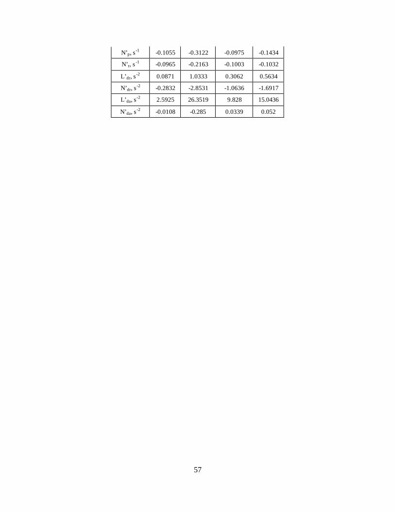
57

N’p, s-1 -0.1055 -0.3122 -0.0975 -0.1434

N’r, s-1 -0.0965 -0.2163 -0.1003 -0.1032

L’dr, s-2 0.0871 1.0333 0.3062 0.5634

N’dr, s-2 -0.2832 -2.8531 -1.0636 -1.6917

L’da, s-2 2.5925 26.3519 9.828 15.0436

N’da, s-2 -0.0108 -0.285 0.0339 0.052

58

THIS PAGE INTENTIONALLY LEFT BLANK

59

APPENDIX E: MATLAB CODE

The following is a listing of the MATLAB, Version 6.0, code used to determine

the P 208’s longitudinal and lateral-directional eigenvalues, roots, natural frequencies,

damping ratios and mode response.

% Longitudinal Dimentional derivatives % P208 Cruise Profile (M=.57, H=29500) % Vorview generated dimensionless derivatives Ix=18143; Iy=12370; Iz=28474; Ixz=200; G=1/(1-Ixz^2/(Ix*Iz)); Q=146.6; U=568.28; S=204.53; b=31.43; c=6.56; m=10300/32.2; M=.57; Cl=0.35; Cd=0.0201; Clalpha=5.4834; ClM=0.1598; Clq=6.9833; Clalphadot=5.5688; Cdalpha=0.4336; CdM=0.10195; Cmalpha= -1.0151; CmM=-0.0228; Cmq=-6.1682; Cmalphadot=-4.9188; Clde=0.3944; Cdde=0.0086; Cmde=-0.6971; Xu=-Q*S/(m*U)*(2*Cd+M*CdM) Xalpha=Q*S*(Cl-Cdalpha)/m Mu=Q*S*c*M*CmM/(Iy*U) Malpha=Q*S*c*Cmalpha/Iy Malphadot=Q*S*c^2*Cmalphadot/(2*U*Iy) Mq=Q*S*c^2*Cmq/(2*U*Iy) Zu=-Q*S/(m*U)*(2*Cl+M*ClM) Zalpha=-Q*S*(Cd+Clalpha)/m Zalphadot=-Q*S*c*Clalphadot/(2*U*m) Zq=-Q*S*c*Clq/(2*U*m)

60

Xde=-Q*S*Cdde/m Mde=Q*S*c*Cmde/Iy Zde=-Q*S*Clde/m A=[Xu Xalpha/U 0 -32.174/U; U*Zu/(U-Zalphadot) Zalpha/(U-Zalphadot) (U+Zq)/(U-Zalphadot) 0; U*Mu+Malphadot*U*Zu/(U-Zalphadot) Malpha+Malphadot*Zalpha/(U-Zalphadot) Mq+Malphadot*(U+Zq)/(U-Zalphadot) 0; 0 0 1 0]; B=[Xde/U;Zde/(U-Zalphadot); Mde+Malphadot*Zde/(U-Zalphadot);0]; b=zeros(4,1); d=zeros(4,1); C=eye(4); p=poly(A) r=roots(p) [Wn,Z]=damp(r) [V,D]=eig(A) %Short period magnitude and phasing MAGshort=abs(V(:,1));PHshort=angle(V(:,1)); magnormalph=MAGshort'/MAGshort(2) %Magnitude relative to alpha phasenormalph=PHshort'-PHshort(2) %Phase relative to alpha in radians Wnshort=Wn(1); %Long period magnatude and phasing MAGlong=abs(V(:,3));PHlong=angle(V(:,3)); magnormu=MAGlong'/MAGlong(1) %Magnitude relative to u/V phasenormu=PHlong'-PHlong(1) %Phase relative to u/V Wnlong=Wn(3); % INITIAL CONDITIONS % Normalized to alpha for short period % Normalized to u/V for long period x0short=[magnormalph.*cos(phasenormalph)+i.*magnormalph.*sin(phasenormalph)]'; x0long=[magnormu.*cos(phasenormu)+i.*magnormu.*sin(phasenormu)]'; sysini=ss(A,B,C,d); x0shortreal=real(x0short); [yshort,tshort,xshort]=initial(sysini,x0shortreal,6); figure plot(tshort(:,1),xshort(:,1),':',tshort(:,1),xshort(:,2),'-',tshort(:,1),xshort(:,3),'- ',tshort(:,1),xshort(:,4),'--') legend('u/V','\alpha','q','\theta') xlabel('Time, sec') ylabel('Response') grid on figure x0longreal=real(x0long);

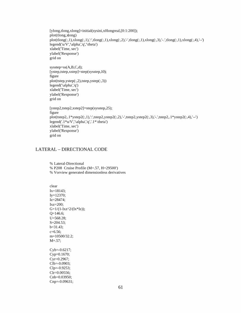
61

[ylong,tlong,xlong]=initial(sysini,x0longreal,[0:1:200]); plot(tlong,xlong) plot(tlong(:,1),xlong(:,1),':',tlong(:,1),xlong(:,2),'-',tlong(:,1),xlong(:,3),'-.',tlong(:,1),xlong(:,4),'--') legend('u/V','\alpha','q','\theta') xlabel('Time, sec') ylabel('Response') grid on sysstep=ss(A,B,C,d); [ystep,tstep,xstep]=step(sysstep,10); figure plot(tstep,ystep(:,2),tstep,ystep(:,3)) legend('\alpha','q') xlabel('Time, sec') ylabel('Response') grid on [ystep2,tstep2,xstep2]=step(sysstep,25); figure plot(tstep2,.1*ystep2(:,1),':',tstep2,ystep2(:,2),'-',tstep2,ystep2(:,3),'-.',tstep2,.1*ystep2(:,4),' --') legend('.1*u/V','\alpha','q','.1*\theta') xlabel('Time, sec') ylabel('Response') grid on

LATERAL – DIRECTIONAL CODE % Lateral-Directional % P208 Cruise Profile (M=.57, H=29500') % Vorview generated dimensionless derivatives clear Ix=18143; Iy=12370; Iz=28474; Ixz=200; G=1/(1-Ixz^2/(Ix*Iz)); Q=146.6; U=568.28; S=204.53; b=31.43; c=6.56; m=10500/32.2; M=.57; Cyb=-0.6217; Cyp=0.1670; Cyr=0.2967; Clb=-0.0903; Clp=-0.9253; Clr=0.00556; Cnb=0.03950; Cnp=-0.09631;

62

Cnr=-0.1096; Cydr=0.09215; Cldr=0.00612; Cndr=-0.0322; Cyda=-0.00517; Clda=0.1892; Cnda=-0.00106; Yb=Q*S*Cyb/m; Yp=Q*S*b*Cyp/(2*U*m); Yr=Q*S*b*Cyr/(2*U*m*Iz); Lb=Q*S*b*Clb/(Ix); Lp=Q*S*b^2*Clp/(2*U*Ix); Lr=Q*S*b^2/(2*U*Ix)*Clr; Nb=Q*S*b*Cnb/Iz; Nr=Q*S*b^2*Cnr/(2*U*Iz); Np=Q* S*b^2*Cnp/(2*U*Iz); Ydr=Q*S*Cydr/m; Yda=Q*S*Cyda/m; Ldr=Q*S*b*Cldr/Ix; Lda=Q*S*b*Clda/Ix; Ndr=Q*S*b*Cndr/Iz; Nda=Q*S*b*Cnda/Iz; Lbpr=(Lb+Nb*(Ixz/Ix))*G; Lppr=(Lp+Np*Ixz/Ix)*G; Lrpr=(Lr+Nr*Ixz/Ix)*G; Nbpr=(Nb+Lb*Ixz/Iz)*G; Nppr=(Np+Lp*Ixz/Iz)*G; Nrpr=(Nr+Lr*Ixz/Iz)*G; Ldrpr=(Ldr+Ndr*Ixz/Ix)*G; Ndrpr=(Ndr+Ldr*Ixz/Iz)*G; Ldapr=(Lda+Nda*Ixz/Ix)*G; Ndapr=(Nda+Lda*Ixz/Iz)*G; A=[Yb/U Yp/U 32.2/U (Yr-U)/U; Lbpr Lppr 0 Lrpr; 0 1 0 0; Nbpr Nppr 0 Nrpr]; Bdr=[Ydr/U;Ldrpr;0;Ndrpr]; Bda=[Yda/U;Ldapr;0;Ndapr]; b=zeros(4,1); d=zeros(4,1); C=eye(4); [V,D]=eig(A) p=poly(A) r=roots(p) [Wn,Z]=damp(r) %Dutch roll values

63

MAGdr=abs(V(:,3));PHdr=angle(V(:,3)); magnormbeta=MAGdr'/MAGdr(1) %Magnitude relative to beta phasenormbeta=PHdr'-PHdr(1) %Phase relative to beta in radians Wndr=Wn(3); %Roll values MAGroll=abs(V(:,1));PHroll=angle(V(:,1)); magnormp=MAGroll'/MAGroll(2) %Magnitude relative to roll rate phasenormp=PHroll'-PHroll(2) %Phase relative to roll rate in radians Wnroll=Wn(1); %Spira l mode MAGspiral=abs(V(:,4));PHspiral=angle(V(:,4)); magnormphi=MAGspiral'/MAGspiral(3) %Magnitude relative to roll angle phasenormphi=PHspiral'-PHspiral(3) %Phase relative to roll angle in radians Wnroll=Wn(4); % Initial Conditions x0dr=[magnormbeta.*cos(phasenormbeta)+i.*magnormbeta.*sin(phasenormbeta)]'; x0roll=[magnormp.*cos(phasenormp)+i.*magnormp.*sin(phasenormp)]'; x0spiral=[magnormphi.*cos(phasenormphi)+i.*magnormphi.*sin(phasenormphi)]'; x0drreal=real(x0dr); x0rollreal=real(x0roll); x0spiralreal=real(x0spiral); sysini=ss(A,b,C,d); syssteprudd=ss(A,Bdr,C,d); figure [ydr,tdr,xdr]=initial(sysini,x0drreal,[0:.01:20]); plot(tdr,xdr(:,1),'-',tdr,xdr(:,2),':',tdr,xdr(:,3),'-.',tdr,xdr(:,4),'--') legend('\beta','p','\phi','r') grid on xlabel('Time (sec)'); ylabel('Response') figure [yroll,troll,xroll]=initial(sysini,x0rollreal,[0:.01:6]); plot(troll,xroll(:,1),'-',troll,xroll(:,2),':',troll,xroll(:,3),'-.',troll,xroll(:,4),'--') legend('\beta','p','\phi','r') grid on xlabel('Time (sec)'); ylabel('Response') figure [yspiral,tspiral,xspiral]=initial(sysini,x0spiralreal,[0:.1:100]); plot(tspiral,xspiral(:,1),'-',tspiral,xspiral(:,2),':',tspiral,xspiral(:,3),'-.',tspiral,xspiral(:,4),'--') legend('\beta','p','\phi','r') grid on xlabel('Time (sec)'); ylabel('Response')

64

[time1,out1]=sim('rudderimp',[0:.1:20]); figure plot(time1,out1(:,1),'-',time1,out1(:,2),':',time1,out1(:,3),'-.',time1,out1(:,4),'--',time1,rudinput); legend('\beta','p','\phi','r','input pulse') grid on xlabel('Time (sec)'); ylabel('Response') [time2,out2]=sim('rudderimp',20); figure plot(time2,out2(:,1),time2,out2(:,3)); hold on legend('\beta','\phi') grid on xlabel('Time (sec)'); ylabel('Response') [time3,out3]=sim('ailimp',[0:.1:20]); figure plot(time3,out3(:,1),time3,out3(:,3),time3,input); legend('\beta','\phi','Input pulse') grid on xlabel('Time (sec)');

65

APPENDIX F: RAM FILE

The following is a listing of the P 208 RAM file. This file should be of use in

future studies.

RAM GEOMETRY FILE 1.05 7 Number 0f Components //***************** WING COMPONENT *****************// //==== General Parms ====// 0 Type Wing Name 0 ID Number 414943041 ID String 4 Color 2 Symmetry Code 4.075 0.000 -0.594 Translation 0.000 2.000 0.000 Rotation //==== Wing Parms ====// 7 Wing Driver Group 9.500000 Span 4.750000 Aspect Ratio 1.000000 Taper Ratio 19.000000 Area 2.000000 Root Chord 2.000000 Tip Chord 0.577350 Tan Sweep 0.250000 Sweep Loc 0.105104 Tan Dihedral 0.000000 Twist Loc 0.000000 Twist 0 Flap Type 0.000000 Flap Inboard Span 1.000000 Flap Outboard Span 0.200000 Flap Chord 0 Slat Type 0.000000 Slat Inboard Span 1.000000 Slat Outboard Span 0.200000 Slat Chord 0 All Move CS //==== Root Airfoil ====// 33 Num of Airfoil Pnts 0.020000 Airfoil Camber 0.400000 Camber Loc 0.120000 Thickness //==== Tip Airfoil ====//

66

33 Num of Airfoil Pnts 0.020000 Airfoil Camber 0.400000 Camber Loc 0.120000 Thickness //***************** FUSE COMPONENT *****************// //==== General Parms ====// 1 Type prop Name 1 ID Number 467012626 ID String 0 Color 0 Symmetry Code 8.500 0.000 0.000 Translation 0.000 0.000 0.000 Rotation //==== Fuse Parms ====// 0.200000 Fuse Length 0.000000 Camber 0.500000 Camber Location 0.000000 Aft Offset 0.000000 Nose Angle 0.300000 Nose Strength 0.790297 Nose Rho 1.686500 Aft Rho 3 Number of Xsecs //==== Cross Section Number 0 ====// 0 Fuse Xsec Type 0.000000 Z_Offset 0.000000 Location On Spine 33 Number of Pnts Per Xsec //==== Cross Section Number 1 ====// 1 Fuse Xsec Type 0.000000 Z_Offset 0.500000 Location On Spine 33 Number of Pnts Per Xsec 3.750000 Height //==== Cross Section Number 2 ====// 0 Fuse Xsec Type 0.000000 Z_Offset 1.000000 Location On Spine 33 Number of Pnts Per Xsec //***************** FUSE COMPONENT *****************// //==== General Parms ====// 1 Type cooler Name 2 ID Number 466757500 ID String 29 Color 0 Symmetry Code 4.123 0.000 -0.892 Translation

67

0.000 0.000 0.000 Rotation //==== Fuse Parms ====// 4.419918 Fuse Length 0.000000 Camber 0.500000 Camber Location 0.000000 Aft Offset 0.000000 Nose Angle 0.300000 Nose Strength 0.640000 Nose Rho 0.809312 Aft Rho 3 Number of Xsecs //==== Cross Section Number 0 ====// 1 Fuse Xsec Type 0.000000 Z_Offset 0.000000 Location On Spine 33 Number of Pnts Per Xsec 0.700000 Height //==== Cross Section Number 1 ====// 1 Fuse Xsec Type 0.000000 Z_Offset 0.250000 Location On Spine 33 Number of Pnts Per Xsec 0.850000 Height //==== Cross Section Number 2 ====// 0 Fuse Xsec Type 0.530000 Z_Offset 1.000000 Location On Spine 33 Number of Pnts Per Xsec //***************** FUSE COMPONENT *****************// //==== General Parms ====// 1 Type Fuselage Name 3 ID Number 415051778 ID String 62 Color 0 Symmetry Code 1.250 0.000 0.000 Translation 0.000 0.000 0.000 Rotation //==== Fuse Parms ====// 8.319942 Fuse Length 0.015000 Camber 0.500000 Camber Location 0.000000 Aft Offset 0.088224 Nose Angle 0.300000 Nose Strength 0.530000 Nose Rho 0.542341 Aft Rho 5 Number of Xsecs //==== Cross Section Number 0 ====// 0 Fuse Xsec Type

68

0.000000 Z_Offset 0.000000 Location On Spine 33 Number of Pnts Per Xsec //==== Cross Section Number 1 ====// 4 Fuse Xsec Type 0.000000 Z_Offset 0.336314 Location On Spine 33 Number of Pnts Per Xsec 1.400000 Height 1.250000 Width 1.200000 Top Tan Strength 1.200000 Upper Tan Strength 1.200000 Lower Tan Strength 1.200000 Bottom Tan Strength -0.646998 Max Width Location 0.500000 Corner Radius 1.570796 Top Tan Angle 1.570796 Bot Tan Angle //==== Cross Section Number 2 ====// 4 Fuse Xsec Type 0.000000 Z_Offset 0.500000 Location On Spine 33 Number of Pnts Per Xsec 1.400000 Height 1.250000 Width 1.200000 Top Tan Strength 1.200000 Upper Tan Strength 1.200000 Lower Tan Strength 1.200000 Bottom Tan Strength -0.646998 Max Width Location 0.500000 Corner Radius 1.570796 Top Tan Angle 1.570796 Bot Tan Angle //==== Cross Section Number 3 ====// 4 Fuse Xsec Type 0.000000 Z_Offset 0.607037 Location On Spine 33 Number of Pnts Per Xsec 1.400000 Height 1.250000 Width 1.200000 Top Tan Strength 1.200000 Upper Tan Strength 1.200000 Lower Tan Strength 1.200000 Bottom Tan Strength -0.646998 Max Width Location 0.500000 Corner Radius 1.570796 Top Tan Angle 1.570796 Bot Tan Angle //==== Cross Section Number 4 ====// 0 Fuse Xsec Type 0.000000 Z_Offset

69

1.000000 Location On Spine 33 Number of Pnts Per Xsec //***************** FUSE COMPONENT *****************// //==== General Parms ====// 1 Type Canopy Name 4 ID Number 415115782 ID String 22 Color 0 Symmetry Code 3.750 0.000 0.530 Translation 0.000 -3.523 0.000 Rotation //==== Fuse Parms ====// 1.967343 Fuse Length 0.003814 Camber 0.225400 Camber Location 0.005210 Aft Offset -0.128401 Nose Angle 0.191410 Nose Strength 0.752160 Nose Rho 0.694896 Aft Rho 3 Number of Xsecs //==== Cross Section Number 0 ====// 0 Fuse Xsec Type 0.000000 Z_Offset 0.000000 Location On Spine 33 Number of Pnts Per Xsec //==== Cross Section Number 1 ====// 2 Fuse Xsec Type 0.000000 Z_Offset 0.342369 Location On Spine 33 Number of Pnts Per Xsec 0.962029 Height 0.808479 Width //==== Cross Section Number 2 ====// 0 Fuse Xsec Type 0.000000 Z_Offset 1.000000 Location On Spine 33 Number of Pnts Per Xsec //***************** FUSE COMPONENT *****************// //==== General Parms ====// 1 Type pod Name 5 ID Number 415328102 ID String 11 Color 2 Symmetry Code 6.800 4.750 -0.170 Translation 0.000 0.000 0.000 Rotation

70

//==== Fuse Parms ====// 4.000000 Fuse Length 0.000000 Camber 0.500000 Camber Location 0.000000 Aft Offset 0.000000 Nose Angle 0.300000 Nose Strength 0.640000 Nose Rho 0.640000 Aft Rho 5 Number of Xsecs //==== Cross Section Number 0 ====// 0 Fuse Xsec Type 0.000000 Z_Offset 0.000000 Location On Spine 33 Number of Pnts Per Xsec //==== Cross Section Number 1 ====// 1 Fuse Xsec Type 0.000000 Z_Offset 0.250000 Location On Spine 33 Number of Pnts Per Xsec 0.300000 Height //==== Cross Section Number 2 ====// 1 Fuse Xsec Type 0.000000 Z_Offset 0.500000 Location On Spine 33 Number of Pnts Per Xsec 0.300000 Height //==== Cross Section Number 3 ====// 1 Fuse Xsec Type 0.000000 Z_Offset 0.750000 Location On Spine 33 Number of Pnts Per Xsec 0.300000 Height //==== Cross Section Number 4 ====// 0 Fuse Xsec Type 0.000000 Z_Offset 1.000000 Location On Spine 33 Number of Pnts Per Xsec //***************** WING COMPONENT *****************// //==== General Parms ====// 0 Type empennage Name 6 ID Number 415366934 ID String 4 Color 2 Symmetry Code 8.942 4.750 -0.180 Translation 0.000 -3.500 0.000 Rotation //==== Wing Parms ====// 5 Wing Driver Group

71

3.400000 Span 3.238095 Aspect Ratio 0.354839 Taper Ratio 3.570000 Area 1.550000 Root Chord 0.550000 Tip Chord 0.431289 Tan Sweep 0.250000 Sweep Loc -0.363970 Tan Dihedral 0.000000 Twist Loc 0.000000 Twist 0 Flap Type 0.000000 Flap Inboard Span 1.000000 Flap Outboard Span 0.200000 Flap Chord 0 Slat Type 0.000000 Slat Inboard Span 1.000000 Slat Outboard Span 0.200000 Slat Chord 0 All Move CS //==== Root Airfoil ====// 33 Num of Airfoil Pnts 0.000000 Airfoil Camber 0.000000 Camber Loc 0.100000 Thickness //==== Tip Airfoil ====// 33 Num of Airfoil Pnts 0.000000 Airfoil Camber 0.000000 Camber Loc 0.100000 Thickness //************* AERO PARMS *************// 0 Wing Reference Component (ID #/Name) 1.000000 Reference Area 1.000000 Reference Span 1.000000 Reference Chord 5.947 0.000 0.000 C.G. Location -1 None Trimming Component (ID #/Name)

72

THIS PAGE INTENTIONALLY LEFT BLANK

73

APPENDIX G: ACSYNT

The P 208 ACSYNT file is given below with initial simple analysis results.

Started at: Fri Mar 8 15:35:47 P ST 2002 Engine Files: /u/wk/ahahn/projects/erast/perseus/acsynt/matched/prop/Convert_to_new_acsynt/P208C copied to fort.3 (Lewis File) /u/wk/ahahn/projects/erast/perseus/acsynt/matched/prop/Convert_to_new_acsynt/P208C copied to fort.9 (Ames File) Note: The above link(s) do not necessarily indicated the engine file was used. The type of engine used depends on the engine settings in the Trajectory portion of the ACSYNT input file (MMPROP, IP). ################################################################################ # # # JOB TITLE # # # ################################################################################ $JOB TITLE = 'p208A' $END ################################################################################ # # # ACSYNT CONTROL # # # ################################################################################ A NEGATIVE NUMBER FOR AN MEXEC INPUT INDICATES THAT MODULE WILL ONLY BE EXECUTED AFTER WEIGHT CONVERGENCE. CONVERGE SET TO .TRUE. INDICATES A WEIGHT CONVERGENCE RUN, SET TO .FALSE. INDICATES A SINGLE PASS RUN. $ACSYNT CONVERGE = .FALSE. MREAD = 5, NREAD = 1, 2, 3, 4, 6, 14, 7, 9, MEXEC = 3, NEXEC = 1, 2, 6, 7, -14, -9, MWRITE = 5, NWRITE = 1, 2, 3, 6, 4, 7, 14, 9, TOL = 0.00010, SLOPE = 0.75, WGMAX = 25000.0, IPSUM = 1, KGLOBP = 0, INIT = 0, IPDBG = 0, IGPLT = 1, IRDDTR = 7, IPDTR = 0, MAXTHRUST = 0., G4FIXWOS = 0. EXTMAX = 0.2, NUMCON = 0, $END ################################################################################ # # # GEOMETRY NAMELISTS # # # ################################################################################ $FUS BDMAX = 4.25, BODL = 26.4, FRAB = 2.5, FRN = 3.7, FRATIO = 6.5, SFFACT = 1.18, ITAIL = 1, OUTCOD = 3, $END $WING AR = 4.75, AREA = 204.53, DIHED = 6.0, FDENWG = 43.0, LFLAPC = 0.00, SWEEP = 30.0, SWFACT = 1.05, TAPER = 0.99, TCROOT = 0.18, TCTIP = 0.12, TFLAPC = 0.25, WFFRAC = 0.9, XWING = 0.346, ZROOT = -0.594, KSWEEP = 1,

74

$END $HTAIL AR = 3.24, AREA = 38.39, SWEEP = 23.33, SWFACT = 1.68, TAPER = 0.35, TCROOT = 0.10, TCTIP = 0.10, XHTAIL = 1.103, ZROOT = -0.5, KSWEEP = 1, SIZIT = .FALSE., HTFRAC = -0.30, CVHT = 1.0, $END $CREW NCREW = 1, $END $FUEL DEN = 43.0, FRAC = 0.9, $END $ENGINE N = 1, $END ################################################################################ # # # TRAJECTORY INPUTS # # # ################################################################################ $TRDATA CRMACH = 0.47, QMAX = 425.0, DESLF = 6.0, ULTLF = 9.0, WFUEL = 1323.0, WFEXT = 0.0, WFTRAP = 50.0, FRFURE = 0.05, IPSTO1 = 5, TIMTO1 = 5.0, IPSTO2 = 2, TIMTO2 = 1.0, IPSLND = 5, MODLND = 7, VMRGLD = 1.2, WKLAND = 0.75, RCTOC = 500., XDESC = 100.0, DECEL=0.25, IBREG = 0, IENDUR = 0, WCOMBP = 0.6, MMPROP = 7, NCODE = 0, NCRUSE = 2, RANGE = 820.0, LEGRES = 0, NMISS = 1, JDPMIS =.FALSE., LENVEL =.FALSE., NLEGCL = 0, NLEGLO = 0, NLEGCR = 0, IPSIZE = 0, IPRINT = 1, KERROR = 2, $END 1 MACH NO. ALTITUDE HORIZONTAL NO. VIND PHASE START END START END DIST TIME TURN "G"S WKFUEL M IP IX W B A P ------- ---- ---- ----- ----- ------ ----- ---- ----- ------ - -- -- - - - - CLIMB 0.18 0.20 0 29000 45.0 0.0 0.0 160.0 1.0000 1 3 -1 0 0 0 0 ACCEL -1 0.55 -1 -1 0.0 5.0 0.0 0.0 1.0000 1 3 -1 0 0 0 0 CRUISE 0.55 0.55 -1 -1 -1.0 0.0 0.0 0.0 1.0000 1 4 -1 0 0 0 0 COMBAT 0.65 0.65 -1 15000 0.0 20.0 0.0 0.0 0.0300 1 2 0 0 0 0 0 CLIMB 0.20 0.18 0 29000 20.0 0.0 0.0 160.0 1.0000 1 3 -1 0 0 0 0 CRUISE 0.55 0.55 -1 29000 -1.0 0.0 0.0 0.0 1.0000 1 4 -1 0 0 0 0 DESCENT -1 0.30 -1 0 0.0 0.0 0.0 0.0 1.0000 1 5 0 0 0 0 0 ################################################################################ # # # AERODYNAMIC INPUTS # # # ################################################################################ $ACHAR ABOSB=0.0, ALMAX=15.0, AMC=40.0, BDNOSE= 4.25, ISMNDR=0, CLO=0.00053,0.00053,0.00052,0.00052,0.0005,0.00047,0.00045,0.00043,0.00039, 0.00027, CLOW=0.0812,0.0819,0.0831,0.0848,0.0872,0.0906,0.0954,0.1024,0.1141,0.1545, CMO=0.0493,0.0496,0.0502,0.0507,0.0515,0.0525,0.0539,0.0558,0.0582,0.0604, SMNSWP= 0.12, 0.17, 0.30, 0.47, 0.50, 0.57, 0.70, 0.80, 0.90, 1.00, SFWF=.90, ALELJ=2,$END $AMULT ESSF=1.00, FCDF=1.00, FCDL=1.00, FCDRA=10*1.00, FCDO=1.00, FCDW=1.00, FCDWB=1.00, FENG=1.00, FINTF=1.00, FLBCOR=1.00, FLD=1.00, FLECOR=1.00, FMDR=1.00,$END $ATRIM FVCAM = 10*0.89, FLDM = 10*1.072 FLAPI = 0.0, 0.0, 0.0, 0.0, 0.0, 0.0, 0.0, 0.0, 0.0, 0.0, ITRIM = 1, 1, 1, 1, 1, 1, 1, 1, 1, 1, IT = -3.5, CGM=0.32, CFLAP=0.25, SPANF=0.64, IVCAM=1, ALFVC=5.0, $END $ADET ALIN=-5.,-2.,0.,2.,4.,6.,8.,10.,12.,15., ALTV= 0.0,5000.0,10000.0,20000.0,25000.0,29500.0,29500.0,40000.0, CLINPT=0.0,0.0,0.0,0.0,0.0,0.0,0.0,0.0,0.0,0.0,

75

SMN=0.47,0.3,0.4,0.4,0.4,0.47,0.57,0.45,0.17,0.17, ICOD=1, IPLOT=1, ISTRS=0,0,0,0,0,0,0,0,0,0, ITB=0,0,0,0,0,0,0,0,0,0, ITS=0,0,0,0,0,0,0,0,0,0, NALF=10, NMDTL=10, $END $ADRAG CDBMB=10*0.0, CDEXTR=10*0.0, CDTNK=10*0.00, $END $ATAKE CLLAND =1.20, CLTO =1.20, DELFLD = 45.0, DELFTO = 30.0, DELLED = 00.0, DELLTO = 00.0, LDLAND =-1.0, LDTO = -1.0, ALFROT = 18.0, IFLAP=1, $END $APRINT KERROR=2, $END ################################################################################ # # # PROPULSION INPUTS # # # ################################################################################ $PCONTR HNOUT = 0.,0.,29500.,29500.,40000., SMNOUT= 0.17, 0.47, 0.47, 0.57, 0.5, NOUTPT= 5, $END $PENGIN ENGNUM = 1, NTPENG = 3, ESZMCH = 0.00, ESZALT = 0.,XNMAX = 2700 , HPENG = 2071 , SWTENG = 1.1 , HCRIT = 42000 , FSFC = 1.0, $END $PROP AF = 124.5, BL = 4, CLI = 0.366, DPROP = 11.15, FPRW = 1.0, FTHR = 1.0, NTPPRP = 12, PSZMCH = 0.00, PSZALT = 0., $END $PGEAR GR = 1.93, ETR = 0.90, FGRW = 1.0, $END $PENGNC XLENG = 8.42, RLENG = 1.08, DIA1 = 3.2, FT = 0.0, FRPN = 2.25, FRBT = 6, NBDFT = 3.82, ANACHP = 0., DQ = 1.0, $END ################################################################################ # # # WEIGHTS INPUTS # # # ################################################################################ WTYPE = TRANsport --> TRANSPORT = FIGHter --> FIGHTER = BOMBer --> BOMBER = GEAV --> GENERAL AVIATION $OPTS WTYPE = 'FIGH', WTITLE = 'P208 WEIGHTS', WGTO = 11133.5, KERROR = 2, IPRINT = 0, ITAIL = 0, $END $FIXW WTSUM = 11133.5, WBODY = 1168.45, WHT = 154.32, WLG = 749.57, WWING = 1455.05, WFEQ = 1153.02, WPS = 3891.16, WCREW = 220.46, WAMMUN = 308.65, WARM = 709.89, $END ################################################################################ ################################################################################ ################################################################################ ################################################################################ # # # THE FOLLOWING NAMELISTS ARE FOR ADS. UNLESS YOU ARE DOING SENSITIVITY # # ANALYSES OR OPTIMIZATIONS, YOU MAY LEAVE THESE VARIABLES UNTOUCHED. # # #

76

################################################################################ ################################################################################ ################################################################################ ################################################################################ **** Sensitivity and Optimization variables not included, Output follows: Output for Module # 1 --> GEOMETRY ****************************************************************************** FUSELAGE CROSS SECTION SIZING TO ACCOMODATE PAYLOAD PAYLOAD WIDTH.................................... 0.0000E+00 PAYLOAD HEIGHT................................... 0.0000E+00 THICKNESS OF WING ROOT........................... 1.187 MAX THICKNESS OF WING FOR FREE FIT............... 0.0000E+00 DIAMETER REQUIRED FOR WIDTH OF EMBEDDED ENGINES.. 0.0000E+00 DIAMETER REQUIRED FOR HEIGHT OF EMBEDDED ENGINES. 0.0000E+00 DIAMETER REQUIRED TO ENCLOSE BOX................. 1.187 REQUIRED DIAMETER..(MAX OF 3 ABOVE).............. 1.187 RADIUS OF ENGINE POD............................ 0.0000E+00 ANGLE OF ENGINE PLACEMENT (ABOVE HORIZONTAL)..... 0.0000E+00 STAND-OFF DISTANCE (NON-DIMENSIONAL)............. 0.0000E+00 STAND-OFF DISTANCE (FT.) ........................ 0.0000E+00 LOC. OF CENTER OF ENGINE......................... 0.5935 AIRCRAFT INTERNAL ARRANGEMENT ITEM LENGTH INITIAL FINAL ACTUAL REQD STATION STATION DIAM DIAM RADAR 0.000 0.000 0.000 0.000 0.000 CREW 3.500 8.227 11.727 3.500 3.500 FUEL 2.158 11.727 13.885 4.042 NOSE LENGTH................................. 15.73 AFTERBODY BEGINS AT......................... 15.77 OVERALL LENGTH.............................. 26.40 MAX. AFT FUEL LOCATION...................... 21.09 DELTAX DUE TO PAYLOAD AFTERBODY MISMATCH.... 1000. DELTAX DUE TO PAYLOAD-FUEL OVERLAP.......... 1000. DELTAX DUE TO FINENESS RATIO REQ............ 0.5000E-01 ACTUAL-REQUIRED CREW DIAMETER............... 0.7500 ACTUAL-REQUIRED PAYLOAD DIAMETER............ 3.063 ACTUAL-REQUIRED POWER PLANT DIAMETER........ 3.250 WING ROOT THICKNESS IN BODY................. 1.187 FUSELAGE WALL THICKNESS..................... 0.0000E+00 VOLUME OF FORWARD FUEL...................... 27.69 VOLUME OF REAR FUEL......................... 0.0000E+00 ACTUAL-REQUIRED FUEL VOLUME................. 31.66 Fuselage Definition (Type 2) Nose Length.................. 15.725 Nose Fineness Ratio.......... 3.700 Constant Section Length...... 0.050 Afterbody Length............. 10.625 Afterbody Fineness Ratio..... 2.500 Overall Length............... 26.400 Maximum Diameter............. 4.250 Body Planform Area........... 68.526 Fuselage Definition X R Area 3.15 0.99 3.06 3.93 1.14 4.11 4.72 1.28 5.17 5.50 1.41 6.23 6.29 1.52 7.26 7.08 1.62 8.26 7.86 1.71 9.21 8.65 1.79 10.10

77

9.44 1.86 10.92 10.22 1.93 11.66 11.01 1.98 12.31 11.79 2.02 12.88 12.58 2.06 13.34 13.37 2.09 13.71 14.15 2.11 13.97 14.94 2.12 14.13 10.46 1.71 9.21 10.99 1.79 10.10 11.52 1.86 10.92 12.06 1.93 11.66 12.59 1.98 12.31 13.12 2.02 12.88 13.65 2.06 13.34 14.18 2.09 13.71 14.71 2.11 13.97 15.24 2.12 14.13 15.77 2.12 14.19 16.31 2.12 14.13 16.84 2.11 13.97 17.37 2.09 13.71 17.90 2.06 13.34 18.43 2.02 12.88 18.96 1.98 12.31 19.49 1.93 11.66 20.02 1.86 10.92 20.56 1.79 10.10 21.09 1.71 9.21 0.00 0.00 0.00 0.00 0.00 0.00 0.00 0.00 0.00 0.00 0.00 0.00 0.00 0.00 0.00 0.00 0.00 0.00 0.00 0.00 0.00 0.00 0.00 0.00 0.00 0.00 0.00 0.00 0.00 0.00 Fuselage Max. Diameter...... 4.250 Fineness Ratio..... 6.212 Surface Area....... 387.844 Volume............. 200.543 Dimensions of Planar Surfaces (each) Wing H.Tail V.Tail Canard Units NUMBER OF SURFACES. 1.0 1.0 1.0 1.0 PLAN AREA.......... 204.5 38.4 0.0 0.0 (SQ.FT.) SURFACE AREA....... 386.5 73.1 0.0 0.0 (SQ.FT.) VOLUME............. 137.8 6.9 0.0 0.0 (CU.FT.) SPAN............... 31.169 11.153 0.000 0.000 (FT.) L.E. SWEEP......... 30.045 30.109 0.000 0.000 (DEG.) C/4 SWEEP.......... 30.000 23.330 0.000 0.000 (DEG.) T.E. SWEEP......... 29.863 -0.832 0.000 0.000 (DEG.) ASPECT RATIO ...... 4.750 3.240 0.000 0.000 ROOT CHORD......... 6.595 5.100 0.000 0.000 (FT.) ROOT THICKNESS..... 14.245 6.119 0.000 0.000 (IN.) ROOT T/C .......... 0.180 0.100 0.000 0.000 TIP CHORD.......... 6.529 1.785 0.000 0.000 (FT.) TIP THICKNESS...... 9.402 2.142 0.000 0.000 (IN.) TIP T/C ........... 0.120 0.100 0.000 0.000 TAPER RATIO ....... 0.990 0.350 0.000 0.000 MEAN AERO CHORD.... 6.562 3.708 0.000 0.000 (FT.) LE ROOT AT......... 7.486 24.020 0.000 0.000 (FT.) C/4 ROOT AT........ 9.134 25.295 0.000 0.000 (FT.)

78

TE ROOT AT......... 14.081 29.119 0.000 0.000 (FT.) LE M.A.C. AT....... 11.985 25.377 0.000 0.000 (FT.) C/4 M.A.C. AT...... 13.626 26.304 0.000 0.000 (FT.) TE M.A.C. AT....... 18.547 29.085 0.000 0.000 (FT.) Y M.A.C. AT........ 7.779 2.341 0.000 0.000 LE TIP AT.......... 16.500 27.253 0.000 0.000 (FT.) C/4 TIP AT......... 18.132 27.700 0.000 0.000 (FT.) TE TIP AT.......... 23.029 29.038 0.000 0.000 (FT.) ELEVATION.......... -1.262 -1.062 0.000 0.000 (FT.) GEOMETRIC TOTAL VOLUME COEFF 0.410 0.000 0.000 REQUESTED TOTAL VOLUME COEFF 0.410 0.000 0.000 ACTUAL TOTAL VOLUME COEFF 0.410 0.000 0.000 E X T E N S I O N S Strake Rear Extension Centroid location at....... 0.00 0.00 Area....................... 0.00 0.00 Sweep Angle................ 0.00 0.00 Wetted Area................ 0.00 0.00 Volume..................... 0.00 0.00 Total Wing Area............ 204.53 Total Wetted Area.......... 847.36 F U E L T A N K S Tank Volume Weight Density Wing 62. 2685. 43.00 Fus#1 0. 0. 43.00 Fus#2 0. 0. 50.00 Total 2685. Mission Fuel Required = 1323. lbs. Extra Fuel Carrying Capability = 1362. lbs. Available Fuel Volume in Wing = 62. cu.ft. Aircraft Weight = 11133.500 lbs. Aircraft Volume = 345.190 cu.ft. Aircraft Density = 32.253 lbs./cu.ft. Actual - Required Fuel Volume = 31.665 cu.ft. ICASE = 8 (Fineness Ratio Method) Output for Module # 2 --> TRAJECTORY ****************************************************************************** Trajectory Output Mission 1 (PAYLOAD = 1019. LB) PHASE M H CL ALPHA WFUEL TIME VEL SFC(I) THRUST(I) CD GAMMA W WA Q SFC(U) THRUST(U) CDINST L/D THR/THA PR X WARM-UP 0. 15.6 5.00 0.13 1443. TAKEOFF 0.14 0. 2.0812 21.76 13.6 1.00 153. -0.02 -53631. 0.4949 90.00 11117.9 0.00 28. -0.02 -53631. 0.0000 4.21 0.45 1.00 1350. 2ND SEG 0.14 400. 2.0812 21.76 153. -0.02 0. 0.4949 14.76 11117.9 0.00 28. -0.02 -53631. 0.0000 4.21 0.45 1.00 CLIMB 0.00 0. 0.0000 0.00 0.0 0.00 0.

79

0.00 0. 0.0000 0.00 0.0 0.00 0. Cycle 0.00 0. 0.0000 0.00nan 0.00 0. LANDING 0.00 0. 0.0000 0.00 0. 0.00 0. 0.0000 0.00 0.0 0.00 0. 0.00 0. 0.0000 0.00 0.00 1.00 0. Fuel Summary Total Fuel = 1323. Takeoff Fuel: Fuel Load: Mission Fuel = 0. Warmup = 16. External = 0. Reserve Fuel = 0. Takeoff = 14. Internal = 1323. Trapped Fuel = 50. Block Time = 0.100 hrs Block Range = 0.0 n.m. Block Fuel = 0.0 lb. FAR Takeoff Field Length = 1350. ft Factor = 1.00 Landing Field Length (total run) = 0. ft Decel @ .250 Gs Landing Field Length (ground run) = 0. ft Field Length Factor = 0.600 Weight for Landing calculation = 0. lbs Landing Thrust to Weight ratio = 0.000 Takeoff Weight = 11134. lbs Landing Weight = 11104. lbs

80

Output for Module # 3 --> AERODYNAMICS ****************************************************************************** Mach = 0.17 C.G. Location = 14.1 ft, 0.32 cbar Q = 42.8 Cj = 0.00 per engine Altitude = 0. Takeoff Configuration: Flaps and Slats Thrust = 0. per engine Parasite Drag Induced Drag Friction .0142 Alpha Cl Cd L/D PF e Zone Cm Cdtrim Deltrim StMrg Body .0055 -6.0 0.324 0.0187 17.4 9.9 2.22 2 0.000 -.0067 8.1 0.055 Wing .0072 -2.9 0.570 0.0390 14.6 11.0 0.93 2 0.000 -.0084 7.3 0.048 Strakes .0000 -0.8 0.745 0.0687 10.8 9.4 0.70 2 0.000 -.0093 6.7 0.049 H. Tail .0015 1.2 0.887 0.0986 9.0 8.5 0.63 2 0.000 -.0095 6.0 0.058 V. Tail .0000 3.3 1.025 0.1301 7.9 8.0 0.61 2 0.000 -.0093 5.3 0.069 Canard .0000 5.4 1.158 0.1651 7.0 7.6 0.60 2 0.000 -.0086 4.4 0.081 Interference .0020 7.5 1.288 0.2011 6.4 7.3 0.60 2 0.000 -.0076 3.6 0.093 Base .0000 9.6 1.414 0.2379 5.9 7.1 0.60 2 0.000 -.0063 2.8 0.107 Wing-Body .0009 11.7 1.537 0.2753 5.6 6.9 0.61 2 0.000 -.0049 2.0 0.121 Wing-Nacelle .0000 14.9 1.718 0.3355 5.1 6.7 0.62 2 0.000 -.0022 0.9 0.141 Excressence .0011 Wave .0000 External .0000 Slope Factors Tanks .0000 Cl/Alpha (per radian) 3.8327 Bombs .0000 Cdl/Cl^2 0.1083 Stores .0000 Alpha Transition Zone 2-3 46.935 Extra .0000 Camber .0007 Flap Setting 30. ___________________ Slat Setting 0. Cdmin .0170 Flap Type Single 26. sq. ft Mach = 0.17 C.G. Location = 14.1 ft, 0.32 cbar Q = 42.8 Cj = 0.00 per engine Altitude = 0. Landing Configuration: Flaps and Slats Thrust = 0. per engine Parasite Drag Induced Drag Friction .0142 Alpha Cl Cd L/D PF e Zone Cm Cdtrim Deltrim StMrg Body .0055 -5.8 0.589 0.0234 25.1 19.3 2.92 2 0.000 -.0078 6.9 0.050 Wing .0072 -2.7 0.833 0.0777 10.7 9.8 0.75 2 0.000 -.0089 6.1 0.045 Strakes .0000 -0.7 1.004 0.1239 8.1 8.1 0.62 2 0.000 -.0097 5.7 0.042 H. Tail .0015 1.3 1.130 0.1679 6.7 7.2 0.56 2 0.000 -.0100 5.4 0.047 V. Tail .0000 3.4 1.254 0.2135 5.9 6.6 0.53 2 0.000 -.0096 4.7 0.059 Canard .0000 5.5 1.375 0.2620 5.2 6.2 0.51 2 0.000 -.0084 3.8 0.071 Interference .0020 7.6 1.492 0.3109 4.8 5.9 0.50 2 0.000 -.0069 2.9 0.085 Base .0000 9.7 1.606 0.3600 4.5 5.7 0.50 2 0.000 -.0052 2.0 0.099 Wing-Body .0009 11.8 1.719 0.4091 4.2 5.5 0.50 2 0.000 -.0033 1.2 0.115 Wing-Nacelle .0000 15.0 1.885 0.4823 3.9 5.4 0.51 2 0.000 -.0005 0.2 0.137 Excressence .0011 Wave .0000 External .0000 Slope Factors Tanks .0000 Cl/Alpha (per radian) 3.5792 Bombs .0000 Cdl/Cl^2 0.1314 Stores .0000 Alpha Transition Zone 2-3 46.935 Extra .0000 Camber .0007 Flap Setting 45. ___________________ Slat Setting 0. Cdmin .0170 Flap Type Single 26. sq. ft

81

Detailed Aerodynamics Output Mach = 0.47 C.G. Location = 14.1 ft, 0.32 cbar Altitude = 0. Reynolds Number per foot = 3.336x10^6 Parasite Drag Induced Drag Friction .0139 Alpha Cl Cd L/D PF e Zone Cm Cdtrim Deltrim StMrg Body .0054 -6.2 -.361 0.0378 -9.6 5.7 0.39 2 0.000 0.0024 9.0 0.090 Wing .0070 -3.1 -.114 0.0227 -5.0 nan 0.11 2 0.000 -.0003 8.0 0.091 Strakes .0000 -1.0 0.061 0.0186 3.3 0.8 0.07 2 0.000 -.0019 7.3 0.093 H. Tail .0015 1.1 0.238 0.0198 12.0 5.9 0.81 2 0.000 -.0031 6.5 0.101 V. Tail .0000 3.2 0.407 0.0266 15.3 9.8 0.97 2 0.000 -.0039 5.6 0.110 Canard .0000 5.3 0.571 0.0381 15.0 11.3 0.95 2 0.000 -.0043 4.8 0.119 Interference .0020 7.4 0.729 0.0530 13.8 11.8 0.94 2 0.000 -.0042 3.9 0.129 Base .0000 9.6 0.883 0.0729 12.1 11.4 0.90 2 0.000 -.0038 3.0 0.139 Wing-Body .0009 11.7 1.032 0.0971 10.6 10.8 0.87 2 0.000 -.0029 2.1 0.149 Wing-Nacelle .0000 14.9 1.250 0.1409 8.9 9.9 0.83 2 0.000 -.0008 0.5 0.163 Excressence .0011 Wave .0000 External .0000 Slope Factors Tanks .0000 Cl/Alpha (per radian) 4.3697 Bombs .0000 Cdl/Cl^2 0.0806 Stores .0000 Alpha Transition Zone 2-3 16.064 Extra .0000 Camber .0008 Programmed Flap Setting 0. ___________________ Cdmin .0167 Flap Type Single 26. sq. ft Mach = 0.30 C.G. Location = 14.1 ft, 0.32 cbar Altitude = 5000. Reynolds Number per foot = 1.853x10^6 Parasite Drag Induced Drag Friction .0141 Alpha Cl Cd L/D PF e Zone Cm Cdtrim Deltrim StMrg Body .0055 -6.2 -.347 0.0369 -9.4 5.5 0.37 2 0.000 0.0021 8.5 0.079 Wing .0071 -3.1 -.109 0.0227 -4.8 nan 0.11 2 0.000 -.0003 7.7 0.080 Strakes .0000 -1.0 0.059 0.0187 3.2 0.8 0.07 2 0.000 -.0018 7.2 0.082 H. Tail .0015 1.1 0.229 0.0197 11.6 5.6 0.81 2 0.000 -.0030 6.5 0.090 V. Tail .0000 3.2 0.392 0.0259 15.2 9.5 0.98 2 0.000 -.0039 5.8 0.099 Canard .0000 5.3 0.549 0.0364 15.1 11.2 0.96 2 0.000 -.0044 5.1 0.109 Interference .0020 7.4 0.702 0.0500 14.0 11.8 0.95 2 0.000 -.0045 4.4 0.119 Base .0000 9.5 0.850 0.0685 12.4 11.4 0.91 2 0.000 -.0043 3.6 0.129 Wing-Body .0009 11.6 0.994 0.0909 10.9 10.9 0.88 2 0.000 -.0037 2.7 0.140 Wing-Nacelle .0000 14.8 1.204 0.1318 9.1 10.0 0.83 2 0.000 -.0021 1.4 0.154 Excressence .0011 Wave .0000 External .0000 Slope Factors Tanks .0000 Cl/Alpha (per radian) 4.2381 Bombs .0000 Cdl/Cl^2 0.0803 Stores .0000 Alpha Transition Zone 2-3 26.129 Extra .0000 Camber .0008 Programmed Flap Setting 0. ___________________ Cdmin .0169 Flap Type Single 26. sq. ft

82

Detailed Aerodynamics Output Mach = 0.40 C.G. Location = 14.1 ft, 0.32 cbar Altitude = 10000. Reynolds Number per foot = 2.140x10^6 Parasite Drag Induced Drag Friction .0140 Alpha Cl Cd L/D PF e Zone Cm Cdtrim Deltrim StMrg Body .0055 -6.2 -.353 0.0373 -9.5 5.6 0.38 2 0.000 0.0023 8.7 0.086 Wing .0071 -3.1 -.111 0.0227 -4.9 nan 0.11 2 0.000 -.0003 7.9 0.087 Strakes .0000 -1.0 0.061 0.0187 3.3 0.8 0.07 2 0.000 -.0019 7.3 0.089 H. Tail .0015 1.1 0.234 0.0198 11.9 5.7 0.81 2 0.000 -.0031 6.5 0.097 V. Tail .0000 3.2 0.401 0.0263 15.2 9.6 0.97 2 0.000 -.0039 5.7 0.106 Canard .0000 5.3 0.561 0.0374 15.0 11.3 0.95 2 0.000 -.0043 4.9 0.115 Interference .0020 7.4 0.717 0.0516 13.9 11.8 0.95 2 0.000 -.0044 4.1 0.125 Base .0000 9.5 0.868 0.0709 12.2 11.4 0.91 2 0.000 -.0040 3.3 0.135 Wing-Body .0009 11.7 1.014 0.0942 10.8 10.8 0.87 2 0.000 -.0032 2.3 0.145 Wing-Nacelle .0000 14.9 1.228 0.1366 9.0 10.0 0.83 2 0.000 -.0013 0.9 0.160 Excressence .0011 Wave .0000 External .0000 Slope Factors Tanks .0000 Cl/Alpha (per radian) 4.3021 Bombs .0000 Cdl/Cl^2 0.0805 Stores .0000 Alpha Transition Zone 2-3 19.206 Extra .0000 Camber .0008 Programmed Flap Setting 0. ___________________ Cdmin .0168 Flap Type Single 26. sq. ft Mach = 0.40 C.G. Location = 14.1 ft, 0.32 cbar Altitude = 20000. Reynolds Number per foot = 1.581x10^6 Parasite Drag Induced Drag Friction .0140 Alpha Cl Cd L/D PF e Zone Cm Cdtrim Deltrim StMrg Body .0055 -6.2 -.355 0.0374 -9.5 5.7 0.38 2 0.000 0.0023 8.7 0.086 Wing .0071 -3.1 -.112 0.0227 -4.9 nan 0.11 2 0.000 -.0003 7.9 0.087 Strakes .0000 -1.0 0.060 0.0186 3.2 0.8 0.07 2 0.000 -.0019 7.3 0.089 H. Tail .0015 1.1 0.233 0.0197 11.8 5.7 0.81 2 0.000 -.0031 6.5 0.097 V. Tail .0000 3.2 0.400 0.0262 15.2 9.6 0.97 2 0.000 -.0039 5.7 0.106 Canard .0000 5.3 0.560 0.0373 15.0 11.3 0.95 2 0.000 -.0043 4.9 0.115 Interference .0020 7.4 0.716 0.0515 13.9 11.8 0.95 2 0.000 -.0044 4.1 0.125 Base .0000 9.5 0.866 0.0707 12.3 11.4 0.91 2 0.000 -.0040 3.3 0.135 Wing-Body .0009 11.7 1.013 0.0940 10.8 10.9 0.87 2 0.000 -.0032 2.3 0.145 Wing-Nacelle .0000 14.9 1.226 0.1362 9.0 10.0 0.83 2 0.000 -.0014 0.9 0.160 Excressence .0011 Wave .0000 External .0000 Slope Factors Tanks .0000 Cl/Alpha (per radian) 4.3021 Bombs .0000 Cdl/Cl^2 0.0804 Stores .0000 Alpha Transition Zone 2-3 19.213 Extra .0000 Camber .0008 Programmed Flap Setting 0. ___________________ Cdmin .0168 Flap Type Single 26. sq. ft

83

Detailed Aerodynamics Output Mach = 0.40 C.G. Location = 14.1 ft, 0.32 cbar Altitude = 25000. Reynolds Number per foot = 1.347x10^6 Parasite Drag Induced Drag Friction .0140 Alpha Cl Cd L/D PF e Zone Cm Cdtrim Deltrim StMrg Body .0055 -6.2 -.354 0.0374 -9.5 5.6 0.38 2 0.000 0.0023 8.7 0.086 Wing .0071 -3.1 -.112 0.0227 -4.9 nan 0.11 2 0.000 -.0003 7.9 0.087 Strakes .0000 -1.0 0.061 0.0187 3.2 0.8 0.07 2 0.000 -.0019 7.3 0.089 H. Tail .0015 1.1 0.234 0.0197 11.8 5.7 0.81 2 0.000 -.0031 6.5 0.097 V. Tail .0000 3.2 0.400 0.0263 15.2 9.6 0.97 2 0.000 -.0039 5.7 0.106 Canard .0000 5.3 0.561 0.0373 15.0 11.3 0.95 2 0.000 -.0043 4.9 0.115 Interference .0020 7.4 0.716 0.0515 13.9 11.8 0.95 2 0.000 -.0044 4.1 0.125 Base .0000 9.5 0.867 0.0708 12.2 11.4 0.91 2 0.000 -.0040 3.3 0.135 Wing-Body .0009 11.6 1.014 0.0940 10.8 10.9 0.87 2 0.000 -.0032 2.4 0.145 Wing-Nacelle .0000 14.9 1.227 0.1363 9.0 10.0 0.83 2 0.000 -.0014 0.9 0.160 Excressence .0011 Wave .0000 External .0000 Slope Factors Tanks .0000 Cl/Alpha (per radian) 4.3026 Bombs .0000 Cdl/Cl^2 0.0804 Stores .0000 Alpha Transition Zone 2-3 19.210 Extra .0000 Camber .0008 Programmed Flap Setting 0. ___________________ Cdmin .0168 Flap Type Single 26. sq. ft Mach = 0.47 C.G. Location = 14.1 ft, 0.32 cbar Altitude = 29500. Reynolds Number per foot = 1.363x10^6 Parasite Drag Induced Drag Friction .0139 Alpha Cl Cd L/D PF e Zone Cm Cdtrim Deltrim StMrg Body .0054 -6.2 -.361 0.0378 -9.6 5.8 0.39 2 0.000 0.0024 8.9 0.090 Wing .0070 -3.1 -.114 0.0227 -5.0 nan 0.11 2 0.000 -.0003 8.0 0.091 Strakes .0000 -1.0 0.061 0.0186 3.3 0.8 0.07 2 0.000 -.0019 7.3 0.093 H. Tail .0015 1.1 0.238 0.0198 12.0 5.9 0.81 2 0.000 -.0031 6.5 0.101 V. Tail .0000 3.2 0.408 0.0266 15.3 9.8 0.97 2 0.000 -.0039 5.7 0.110 Canard .0000 5.3 0.571 0.0381 15.0 11.3 0.95 2 0.000 -.0043 4.8 0.119 Interference .0020 7.4 0.729 0.0529 13.8 11.8 0.94 2 0.000 -.0043 3.9 0.129 Base .0000 9.6 0.882 0.0728 12.1 11.4 0.90 2 0.000 -.0038 3.0 0.139 Wing-Body .0009 11.7 1.031 0.0969 10.6 10.8 0.87 2 0.000 -.0029 2.1 0.149 Wing-Nacelle .0000 14.9 1.248 0.1404 8.9 9.9 0.83 2 0.000 -.0008 0.5 0.163 Excressence .0011 Wave .0000 External .0000 Slope Factors Tanks .0000 Cl/Alpha (per radian) 4.3657 Bombs .0000 Cdl/Cl^2 0.0805 Stores .0000 Alpha Transition Zone 2-3 16.064 Extra .0000 Camber .0008 Programmed Flap Setting 0. ___________________ Cdmin .0167 Flap Type Single 26. sq. ft

84

Detailed Aerodynamics Output Mach = 0.57 C.G. Location = 14.1 ft, 0.32 cbar Altitude = 29500. Reynolds Number per foot = 1.653x10^6 Parasite Drag Induced Drag Friction .0138 Alpha Cl Cd L/D PF e Zone Cm Cdtrim Deltrim StMrg Body .0054 -6.2 -.369 0.0383 -9.6 5.8 0.39 2 0.000 0.0026 9.4 0.096 Wing .0069 -3.1 -.113 0.0226 -5.0 nan 0.11 2 0.000 -.0003 8.3 0.097 Strakes .0000 -0.9 0.069 0.0185 3.7 1.0 0.09 2 0.000 -.0021 7.5 0.098 H. Tail .0015 1.1 0.252 0.0201 12.5 6.3 0.81 2 0.000 -.0033 6.6 0.106 V. Tail .0000 3.2 0.427 0.0276 15.5 10.1 0.96 2 0.000 -.0041 5.7 0.114 Canard .0000 5.4 0.596 0.0401 14.9 11.5 0.94 2 0.000 -.0044 4.7 0.124 Interference .0020 7.5 0.759 0.0560 13.5 11.8 0.94 2 0.000 -.0042 3.8 0.133 Base .0000 9.6 0.917 0.0773 11.9 11.4 0.90 2 0.000 -.0036 2.8 0.143 Wing-Body .0009 11.8 1.070 0.1029 10.4 10.8 0.87 2 0.000 -.0025 1.7 0.153 Wing-Nacelle .0000 15.1 1.202 0.2273 5.3 5.8 0.46 3 0.000 -.0001 -0.4 0.256 Excressence .0011 Wave .0000 External .0000 Slope Factors Tanks .0000 Cl/Alpha (per radian) 4.2278 Bombs .0000 Cdl/Cl^2 0.1471 Stores .0000 Alpha Transition Zone 2-3 12.804 Extra .0000 Camber .0009 Programmed Flap Setting 0. ___________________ Cdmin .0166 Flap Type Single 26. sq. ft Mach = 0.45 C.G. Location = 14.1 ft, 0.32 cbar Altitude = 40000. Reynolds Number per foot = 0.861x10^6 Parasite Drag Induced Drag Friction .0139 Alpha Cl Cd L/D PF e Zone Cm Cdtrim Deltrim StMrg Body .0054 -6.2 -.360 0.0377 -9.5 5.7 0.38 2 0.000 0.0024 8.9 0.089 Wing .0070 -3.1 -.113 0.0227 -5.0 nan 0.11 2 0.000 -.0003 8.0 0.090 Strakes .0000 -1.0 0.061 0.0186 3.3 0.8 0.07 2 0.000 -.0019 7.3 0.092 H. Tail .0015 1.1 0.237 0.0198 12.0 5.8 0.81 2 0.000 -.0031 6.5 0.100 V. Tail .0000 3.2 0.406 0.0265 15.3 9.7 0.97 2 0.000 -.0039 5.7 0.108 Canard .0000 5.3 0.569 0.0380 15.0 11.3 0.95 2 0.000 -.0043 4.9 0.118 Interference .0020 7.4 0.726 0.0526 13.8 11.8 0.94 2 0.000 -.0043 4.0 0.128 Base .0000 9.5 0.878 0.0722 12.2 11.4 0.91 2 0.000 -.0039 3.1 0.138 Wing-Body .0009 11.7 1.026 0.0960 10.7 10.8 0.87 2 0.000 -.0030 2.2 0.148 Wing-Nacelle .0000 14.9 1.241 0.1390 8.9 9.9 0.83 2 0.000 -.0010 0.6 0.162 Excressence .0011 Wave .0000 External .0000 Slope Factors Tanks .0000 Cl/Alpha (per radian) 4.3476 Bombs .0000 Cdl/Cl^2 0.0804 Stores .0000 Alpha Transition Zone 2-3 16.868 Extra .0000 Camber .0008 Programmed Flap Setting 0. ___________________ Cdmin .0167 Flap Type Single 26. sq. ft

85

Output for Module # 6 --> WEIGHTS ****************************************************************************** Weight Statement - Fighter P208 WEIGHTS Qmax: 425. Design Load Factor: 6.00 Ultimate Load Factor: 9.00 Structure and Material: Alumin um Skin, Stringer Wing Equation: Fixed or Structural Method Body Equation: Fixed or Structural Method Component Pounds Kilograms Percent Slope Tech Fixed Airframe Structure 3340.1 1515.0 30.00 No Wing 1455.1 660.0 13.07 1.00 1.00 Yes Fuselage 1168.4 530.0 10.49 1.00 1.00 Yes Horizontal Tail ( Low) 154.3 70.0 1.39 1.00 1.00 Yes Vertical Tail 111.3 50.5 1.00 1.00 1.00 No Nacelles 111.3 50.5 1.00 1.00 1.00 No Landing Gear 749.6 340.0 6.73 1.00 1.00 Yes Propulsion 3891.2 1765.0 34.95 Yes Engines ( 1) 1224.7 555.5 11.00 1.00 1.00 No Fuel System 311.7 141.4 2.80 1.00 1.00 No Fixed Equipment 1153.0 523.0 10.36 1.00 Yes Hyd & Pneumatic 133.6 60.6 1.20 1.00 No Electrical 278.3 126.3 2.50 1.00 No Avionics 445.3 202.0 4.00 1.00 No Instrumentation 122.5 55.6 1.10 1.00 No De-ice & Air Cond 111.3 50.5 1.00 1.00 No Auxiliary Gear 33.4 15.2 0.30 No Furnish & Eqpt 311.7 141.4 2.80 1.00 No Flight Controls 334.0 151.5 3.00 1.00 No Empty Weight 0.0 0.0 0.00 Operating Items 0.0 0.0 0.00 No Flight Crew ( 1) 220.5 100.0 1.98 Yes Crew Baggage and Provisions 0.0 0.0 0.00 No Unusable Fuel and Oil 50.0 22.7 0.45 No Operating Weight Empty 0.0 0.0 0.00 Fuel 1273.0 577.4 11.43 Payload 1018.5 462.0 9.15 No Armament 709.9 322.0 6.38 Yes Ammunition 308.6 140.0 2.77 Yes Missiles 0.0 0.0 0.00 No Bombs 0.0 0.0 0.00 No External Tanks 0.0 0.0 0.00 No Adv Weapons 1 0.0 0.0 0.00 No Adv Weapons 2 0.0 0.0 0.00 No -------- -------- ------ Calculated Weight 11133.5 5050.2 86.39 Yes Estimated Weight 11133.5 5050.2 Percent Error 0.00 Calculated Weight does not equal 100% because a group weight is being fixed. Output for Module # 4 --> PROPULSION

86

****************************************************************************** Propulsion Output: Engine and Propeller Engine Type:Recipricating Turbocharged to: 42000.0 Sea Level Static HP (each) 2071.0 Max. Shaft Speed (RPM) 2700.00 Multiplier for sfc 1.0000 Spcific D/Q (sq-ft/HP) 1.0000 Weight (lbs) 2278.1 Propeller Type HS Constant Speed Number of Blades 4. Diameter (ft) 11.15 Chord (ft) 0.89 Activity Factor 124.50 Integ. Lift Coef. 0.3660 Solidity 0.2030 Tip Speed (ft/sec) 816.72 Power Loading (HP/ft**2) 19.09 Disk Loading (lb/ft**2) 50.79 Torque (ft lbs) 6997.82 Velocity Slipstream (ft/sec) 206.73 Multiplier for thrust 1.0000 Weight Scale Factor 1.0000 Weight (lbs) 284.2 Gear Reduction Propeller Extrap. Errors Engine/Propeller RPM Ratio 1.9300 Transmission Efficiency 0.9000 2 Advance Ratio 5 Cl integ. Auto. Trans. Shift Alt. 0. 3 Cp 6 Blade Angle Weight Scale Factor 1.0000 Weight (lbs) 440.1 Propulsion System Weight/Engine 3002.4 Engine and Propeller Noise (PNdb) 98.704 Mach Number = 0.17 Altitude = 0. Maximum RPM = 2700. Percent HP/Eng Gear ThrustU ThrustI Bsfc TsfcI FFLOW Tip Advance Prop Cp Ct Blade E Power Loss Mach Ratio effU Angle X ------- ------ ---- ------- ------- ----- ----- ----- ---- ------- ------ ------ ------ ----- - 100.0% 2071.0-207.1 3859. -84803. 0.486 -0.012 1007.5 0.73 0.7322 0.716 0.1975 0.1932 27.50 0 95.0% 1967.4-196.7 3723. -84939. 0.498 -0.012 979.6 0.73 0.7322 0.727 0.1876 0.1864 26.99 0 90.0% 1863.9-186.4 3576. -85086. 0.508 -0.011 947.1 0.73 0.7322 0.737 0.1777 0.1790 26.47 0 80.0% 1656.8-165.7 3273. -85389. 0.528 -0.010 874.2 0.73 0.7322 0.759 0.1580 0.1639 25.38 0 70.0% 1449.7-145.0 2950. -85712. 0.551 -0.009 798.6 0.73 0.7322 0.782 0.1382 0.1477 24.24 0 60.0% 1242.6-124.3 2598. -86064. 0.583 -0.008 725.0 0.73 0.7322 0.804 0.1185 0.1301 23.00 0 50.0% 1035.5-103.6 2216. -86446. 0.631 -0.008 653.5 0.73 0.7322 0.822 0.0987 0.1110 21.73 0 Mach Number = 0.47 Altitude = 0. Maximum RPM = 2700. Percent HP/Eng Gear ThrustU ThrustI Bsfc TsfcI FFLOW Tip Advance Prop Cp Ct Blade E Power Loss Mach Ratio effU Angle X ------- ------ ---- ------- ------- ----- ----- ----- ---- ------- ------ ------ ------ ----- - 100.0% 2071.0-207.1 1762. -675932. 0.486 -0.001 1007.5 0.73 2.0243 0.904 0.1975 0.0882 41.90 3 95.0% 1967.4-196.7 1672. -676022. 0.498 -0.001 979.6 0.73 2.0243 0.903 0.1876 0.0837 41.70 3 90.0% 1863.9-186.4 1583. -676111. 0.508 -0.001 947.1 0.73 2.0243 0.903 0.1777 0.0793 41.49 3 80.0% 1656.8-165.7 1400. -676294. 0.528 -0.001 874.2 0.73 2.0243 0.898 0.1580 0.0701 41.08 3 70.0% 1449.7-145.0 1206. -676488. 0.551 -0.001 798.6 0.73 2.0243 0.884 0.1382 0.0604 40.65 3 60.0% 1242.6-124.3 1017. -676678. 0.583 -0.001 725.0 0.73 2.0243 0.869 0.1185 0.0509 40.21 3 50.0% 1035.5-103.6 792. -676902. 0.631 -0.001 653.5 0.73 2.0243 0.813 0.0987 0.0397 39.79 3 Mach Number = 0.47 Altitude = 29500. Maximum RPM = 2700. Percent HP/Eng Gear ThrustU ThrustI Bsfc TsfcI FFLOW Tip Advance Prop Cp Ct Blade E

87

Power Loss Mach Ratio effU Angle X ------- ------ ---- ------- ------- ----- ----- ----- ---- ------- ------ ------ ------ ----- - 100.0% 2071.0-207.1 1763. -204498. 0.486 -0.005 1007.5 0.82 1.8077 0.808 0.5174 0.2313 46.72 0 95.0% 1967.4-196.7 1693. -204569. 0.498 -0.005 979.6 0.82 1.8077 0.816 0.4915 0.2221 46.17 0 90.0% 1863.9-186.4 1622. -204639. 0.508 -0.005 947.1 0.82 1.8077 0.826 0.4657 0.2128 45.62 0 80.0% 1656.8-165.7 1473. -204788. 0.528 -0.004 874.2 0.82 1.8077 0.844 0.4139 0.1933 44.48 0 70.0% 1449.7-145.0 1319. -204942. 0.551 -0.004 798.6 0.82 1.8077 0.863 0.3622 0.1730 43.31 0 60.0% 1242.6-124.3 1156. -205105. 0.583 -0.004 725.0 0.82 1.8077 0.883 0.3104 0.1517 42.13 0 50.0% 1035.5-103.6 978. -205283. 0.631 -0.003 653.5 0.82 1.8077 0.896 0.2587 0.1283 40.93 0 Mach Number = 0.57 Altitude = 29500. Maximum RPM = 2700. Percent HP/Eng Gear ThrustU ThrustI Bsfc TsfcI FFLOW Tip Advance Prop Cp Ct Blade E Power Loss Mach Ratio effU Angle X ------- ------ ---- ------- ------- ----- ----- ----- ---- ------- ------ ------ ------ ----- - 100.0% 2071.0-207.1 1549. -301821. 0.486 -0.003 1007.5 0.82 2.1923 0.861 0.5174 0.2032 49.26 0 95.0% 1967.4-196.7 1482. -301887. 0.498 -0.003 979.6 0.82 2.1923 0.867 0.4915 0.1945 48.82 0 90.0% 1863.9-186.4 1416. -301954. 0.508 -0.003 947.1 0.82 2.1923 0.874 0.4657 0.1858 48.36 0 80.0% 1656.8-165.7 1272. -302098. 0.528 -0.003 874.2 0.82 2.1923 0.884 0.4139 0.1669 47.44 0 70.0% 1449.7-145.0 1115. -302255. 0.551 -0.003 798.6 0.82 2.1923 0.885 0.3622 0.1463 46.49 0 60.0% 1242.6-124.3 961. -302408. 0.583 -0.002 725.0 0.82 2.1923 0.890 0.3104 0.1261 45.59 0 50.0% 1035.5-103.6 807. -302563. 0.631 -0.002 653.5 0.82 2.1923 0.896 0.2587 0.1058 44.69 0 Mach Number = 0.50 Altitude = 40000. Maximum RPM = 2700. Percent HP/Eng Gear ThrustU ThrustI Bsfc TsfcI FFLOW Tip Advance Prop Cp Ct Blade E Power Loss Mach Ratio effU Angle X ------- ------ ---- ------- ------- ----- ----- ----- ---- ------- ------ ------ ------ ----- - 100.0% 2071.0-207.1 1497. -140982. 0.486 -0.007 1007.5 0.84 1.8673 0.709 0.7992 0.3034 52.76 0 95.0% 1967.4-196.7 1457. -141023. 0.498 -0.007 979.6 0.84 1.8673 0.726 0.7593 0.2952 51.91 0 90.0% 1863.9-186.4 1411. -141068. 0.508 -0.007 947.1 0.84 1.8673 0.742 0.7193 0.2860 51.09 0 80.0% 1656.8-165.7 1308. -141171. 0.528 -0.006 874.2 0.84 1.8673 0.774 0.6394 0.2651 49.53 0 70.0% 1449.7-145.0 1188. -141291. 0.551 -0.006 798.6 0.84 1.8673 0.803 0.5595 0.2408 47.97 0 60.0% 1242.6-124.3 1053. -141427. 0.583 -0.005 725.0 0.84 1.8673 0.830 0.4795 0.2133 46.35 0 50.0% 1035.5-103.6 906. -141574. 0.631 -0.005 653.5 0.84 1.8673 0.857 0.3996 0.1835 44.64 0 Propulsion was called 24 times. Engin routine was called 59 times. Output for Module # 11 --> SUMMARY OUTPUT ****************************************************************************** SUMMARY --- ACSYNT OUTPUT: p208A GENERAL FUSELAGE WING HTAIL VTAIL WG 11134. LENGTH 26.4 AREA 204.5 38.4 0.0 W/S 0.0 DIAMETER 4.2 WETTED AREA 386.5 73.1 0.0 T/W 0.00 VOLUME 200.5 SPAN 31.2 11.2 0.0 N(Z) ULT 9.0 WETTED AREA 387.8 L.E. SWEEP 30.0 30.1 90.0 CREW 1. FINENESS RATIO 6.2 C/4 SWEEP 30.0 23.3 0.0 PASENGERS 0. ASPECT RATIO 4.75 3.24 0.00 TAPER RATIO 0.99 0.35 0.00 ENGINE WEIGHTS T/C ROOT 0.18 0.10 0.00 T/C TIP 0.12 0.10 0.00 NUMBER 1. W WG ROOT CHORD 6.6 5.1 0.0 LENGTH 8.4 STRUCT. 3340. 30.0 TIP CHORD 6.5 1.8 0.0 DIAM. 3.2 PROPUL. 3891. 35.0 M.A. CHORD 6.6 3.7 0.0 WEIGHT 3002.4 FIX. EQ. 1153. 10.4 LOC. OF L.E. 7.5 24.0 0.0 TSLS 4959. FUEL 1323. 11.9 SFCSLS 0.00 PAYLOAD 1019. 9.1 ESF 0.000 OPER IT 0. 0.0 MISSION SUMMARY

88

PHASE MACH ALT FUEL TIME DIST L/D THRUST SFC Q ======= ==== ====== ====== ===== ====== ===== ======= ===== ====== TAKEOFF 0.00 0. 29. 6.0 1349.6 CLIMB 0.00 0. 0. 0.0 0.0 0.00 0.0 0.000 0.0 LANDING 0.0 Block Time = 0.100 hr Block Range = 0.0 nm 1 PROGRAM CALLS TO ANALIZ ICALC CALLS 1 1 2 1 3 1 Finished at: Fri Mar 8 15:35:51 PST 2002 Output for Module: Output for Module # 1 --> GEOMETRY Output for Module # 2 --> TRAJECTORY Output for Module # 3 --> AERODYNAMICS Output for Module # 4 --> PROPULSION Output for Module # 6 --> WEIGHTS Output for Module # 11 --> SUMMARY OUTPUT Warnings and Errors:

89

INITIAL DISTRIBUTION LIST

1. Defense Technical Information Center 8725 John J. Kingman Rd., STE 0944 Ft. Belvoir, VA 22060-6218

2. Dudley Knox Library Naval Postgraduate School 411 Dyer Rd. Monterey, CA 93943-5000

3. Dr. Max F. Platzer, AA/PL Naval Postgraduate School Monterey, CA 93943-5106

4. LT Kurt W. Muller

7787 C Street Chesapeake Beach, MD 20732

5. Dr. Conrad F. Newberry AA/Ne Naval Postgraduate School Monterey, CA 93943-5106

6. Dr. Richard M. Howard AA/Ho Naval Postgraduate School Monterey, CA 93943-5106

7. Dr. Louis V. Schmidt AA/Sc Naval Postgraduate School Monterey, CA 93943-5106

8. Mr. Andrew S. Hahn Systems Analysis Branch MS 237-11

NASA Ames Research Center Moffett Field, CA 94035-1000

90

9. Dr. J.A.C. Kentfield Department of Mechanical Engineering The University of Calgry

Calgary, Alberta, Canada T2N 1N4

10. Mr. Paul Gelhausen System Analysis Branch MS 348

NASA Langley Research Center Hampton, VA 23681-2199