thesis apichat final -...

PERMANENT DEFORMATION OF CLAYEY SOILS INDUCED

BY STATIC UNLOADING-RELOADING CYCLES

Dissertation Submitted to Saga University in Fulfillment of the

Requirement for the Degree of Doctor of Philosophy

by

APICHAT SUDDEEPONG

Dissertation Supervisor: Prof. Jinchun Chai

Examination Committee: Prof. Jinchun Chai

Prof. Koji Ishibashi

Prof. Takenori Hino

Associate Prof. Akira Sakai

External Examiners: Prof. Shuilong Shen

Department of Science and Advanced Technology

Graduate School of Science and Engineering

Saga University

2015

i

ACKNOWLEDGEMENTS

The author would like to express his deepest gratitude to his supervisor, Prof. Jinchun

Chai for his excellent guidance, constructive suggestions, encouragements and constant support

throughout the duration of this study.

The author is also very grateful to Prof. Kouji Isibashi, Prof. Takenori Hino and Assoc.

Prof. Akira Sakai for their help, suggestions and serving as members of the examination

committee. Sincere thanks and appreciation are due to Prof. Shuilong Shen of Shanghai Jiao

Tong University for his help and suggestions as well as serving as external examiner. Thanks are

also extended to Dr. Takehito Negami and the laboratory staff, Mr. Akinori Saito, for their help

and kind assistance in conducting the laboratory tests. The author would like to express his

gratitude to Prof. Takenori Hino for providing the medium Ariake clay samples which have been

used in the laboratory oedometer tests.

The author would like to acknowledgement with appreciation to the Japanese

Government for providing a Monbugakakusho: MEXT which made it possible to pursue his

doctoral studies at Saga University, Saga, Japan.

The author is grateful to the Japan Society for the Promotion of Science for funding the

present research work under Grant-in-Aid for Scientific Research (B) (No. 23360204) and Grant-

in-Aid for Challenging Exploratory Research (No. 23656300).

Sincere thanks are due to his former colleague, Dr. Katrika Sari for her advises and

sincere helps. The author acknowledges his sincerest gratitude to his colleague Mrs. Steeva Gaily

Rondonuwu, Mr. Xu Fang, Mr. Sailesh Shrestha, Mr. Nachanok Chanmee and Mr. Zhou Yang

for their help and encouragement. A word of thanks goes to the secretary in the research team,

Ms. Yasuko Kanada for her kindness help.

The author would like to express his love and sincere gratitude to his parents and elder

brother for their support, understanding and encouraging with their best wish. A special note of

appreciation also goes to his beloved, Haruetai Maskong for her consistent patience,

understanding and encouraging which made his study more than just successful.

iii

ABSTRACT

A series of laboratory oedometer tests were conducted for undisturbed soft and medium

Ariake clay samples and reconstituted Ariake clay samples to investigate the static repeated

unloading-reloading induce plastic deformation of the samples. The items investigated are:

number of repeated unloading-reloading cycles; the effect of small intermediate reloading-

unloading (r-u) cycles on a general unloading path and small intermediate unloading-reloading

(u-r) cycles on a general reloading path; and the effect of strain rate. The test results of single

unloading-reloading cycle indicate that in log�� − log�� plot, unloading path is close to linear,

but reloading path is non-linear. Here � = 1 + � (where � is the void ratio) and ′ is the vertical

consolidation pressure. The test results of repeated unloading-reloading cycles show that even in

overconsolidated region, repeated unloading-reloading cycles induced plastic deformation of the

samples. For reconstituted sample, with a given range of stress change up to 10 unloading-

reloading cycles, the plastic deformation increased almost linearly with the increase of number of

the cycles. However, for microstructured undisturbed sample, when intermediate unloading

pressure (′� ) is the same pressure as the maximum vertical effective stress before the first

unloading (′�), increment of plastic deformation decreased drastically with the increase of the

number of unloading-reloading cycle (�) for � = 1 to 4 due to the destructuring effect. For a

general unloading path, increase the number of small intermediate r-u cycles increased the final

plastic deformation; and for a general reloading path, increase the number of small intermediate

u-r cycles reduced the final plastic deformation. The results of the test with a time interval of 1

day and 7 days between successive loading increments indicate that the test with 7 days time

interval had smaller yield stress, and larger plastic strain.

A model for predicting the plastic deformation induced by repeated unloading-reloading

has been proposed based on Butterfield’s (2011) model. The main modifications are: (1)

considering plastic deformation induced by intermediate (within overconsolidated region)

unloading-reloading cycles; and (2) considering volumetric strain hardening. Also, methods for

determining model parameters have been established. Comparing the simulated and the test

results indicate that the model can predict plastic deformation induced by repeated unloading-

reloading cycles well.

iv

In many regions with clayey soil deposits, there are field measurements show that

seasonal or even daily groundwater fluctuations caused land-subsidence. The effect of

groundwater fluctuations to clayey soil is analogy to repeated unloading-reloading cycles. The

proposed model has been applied to simulate compression of clayey soil deposits induced by

daily fluctuations of pore-water pressure of five case histories, two sites in Saga Plain, Japan;

one site in Yokohama, Japan; and two sites in Bangkok, Thailand. Good agreements between the

measured and simulated compressions of the soil layers have been obtained. Further, comparing

the simulated results with the field measured data indicate that compression of clayey soil layer

was influenced by the small intermediate pore-water pressure variations. Therefore, to correctly

simulate/predict groundwater pressure variations induced compression (settlement) of clayey soil

layers, considering daily pore-water pressure variations is necessary.

v

TABLE OF CONTENTS

ACKNOWLEDGEMENTS ............................................................................................................. i

ABSTRACT ................................................................................................................................... iii

LIST OF FIGURES ....................................................................................................................... ix

LIST OF TABLES ........................................................................................................................ xv

LIST OF NOTATIONS .............................................................................................................. xvii

CHAPTER 1 INTRODUCTION .................................................................................................... 1

1.1 General background .............................................................................................................. 1

1.2 Objective and scopes of study ............................................................................................... 2

1.3 Organization of this study ..................................................................................................... 2

CHAPTER 2 LITERATURE REVIEW ......................................................................................... 3

2.1 Land-subsidence .................................................................................................................... 3

2.2 Mechanism of consolidation cause by pore-water pressure drawdown in an aquifer ......... 11

2.3 Unloading-reloading effect on one-dimensional deformation behaviour ........................... 14

2.4 Strain rate effect on consolidation yield stress (′�) ........................................................... 27

2.5 Summary and remarks ......................................................................................................... 30

CHAPTER 3 LABORATORY EXPERIMENTAL INVESTIGATIONS ................................... 31

3.1 Introduction ......................................................................................................................... 31

3.2 Equipment and the materials used ....................................................................................... 31

vi

3.2.1 Soil samples .................................................................................................................. 31

3.2.2 Oedometer tests ............................................................................................................ 32

3.3 Test procedures ................................................................................................................... 32

3.3.1 Single unloading-reloading........................................................................................... 33

3.3.2 Repeated intermediate unloading-reloading ................................................................. 33

3.4 Results and discussions ....................................................................................................... 37

3.4.1 Single unloading-reloading cycle ................................................................................. 37

3.4.2 Repeated intermediate unloading- reloading cycles ..................................................... 37

3.4.3 Effect of small intermediate unloading-reloading (r-u) and reloading-unloading (u-r) cycle ....................................................................................................................................... 47

3.4.4 Effect of number of unloading-reloading cycles (N) .................................................... 50

3.4.5 Effect of time interval between loading step ................................................................ 50

3.5 Summary ............................................................................................................................. 51

CHAPTER 4 THEORETICAL MODELLING ............................................................................ 55

4.1 Introduction ......................................................................................................................... 55

4.2 Predicting unloading-reloading cycle by Butterfield’s unloading-reloading model ........... 55

4.2.1 Butterfield’s unloading-reloading model...................................................................... 55

4.2.2 Parameter determination method .................................................................................. 56

4.2.3 Comparison of simulated and test results ..................................................................... 57

4.3 Modified unloading-reloading model .................................................................................. 66

4.3.1 Proposed intermediate unloading-reloading curve ....................................................... 66

4.3.2 Parameter determination ............................................................................................... 66

vii

4.4 Simulation of laboratory test ............................................................................................... 71

4.4.1 Repeated intermediate unloading-reloading ................................................................. 71

4.4.2 Small intermediate unloading-reloading ...................................................................... 71

4.5 Proposed method to determine yield stress with a known strain rate ................................. 80

4.6 Summary ............................................................................................................................. 81

CHAPTER 5 APPLICATIONS TO FIELD CASE HISTORIES................................................. 83

5.1 Introduction ......................................................................................................................... 83

5.2 Simulating land-subsidence ................................................................................................. 83

5.2.1 Two sites in Saga Plain, Japan...................................................................................... 83

5.2.2 Yokohama, Japan.......................................................................................................... 93

5.2.3 Two sites in Bangkok, Thailand ................................................................................. 103

5.3 Summary ........................................................................................................................... 111

CHAPTER 6 CONCLUDING REMARKS................................................................................ 113

6.1 Conclusions ....................................................................................................................... 113

6.2 Recommendation for future works .................................................................................... 115

REFFERENCES ......................................................................................................................... 117

ix

LIST OF FIGURES

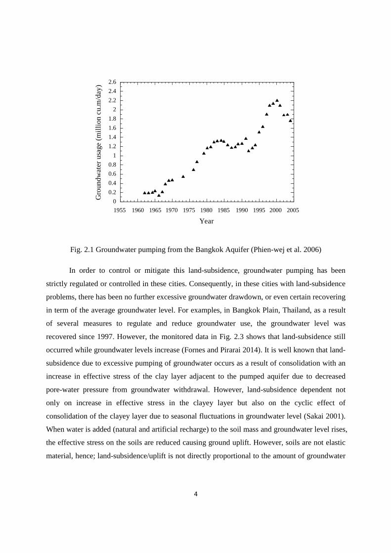
Fig. 2.1 Groundwater pumping from the Bangkok Aquifer (Phien-wej et al. 2006) ...................... 4

Fig. 2.2 Land-subsidence and piezometric drawdowns of Bangkok aquifers versus time (Phien-

wej et al. 2006); (a) Southeastern location (b) Southwestern location .............................. 5

Fig. 2.3 Water level from three major aquifers and total land-subsidence in Central Bangkok

(Fornes and Pirarai 2014) .................................................................................................. 7

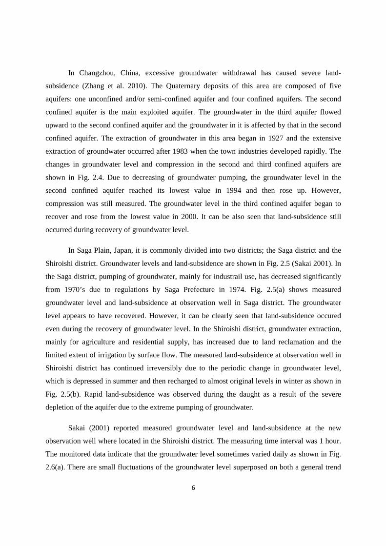
Fig. 2.4 Changes of groundwater level and compression of confined aquifer in Changzhou, China

(Zhang et al. 2010); a) the second confined aquifer b) the third confined aquifer ............ 8

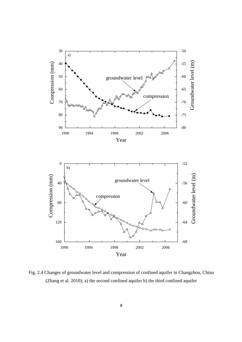
Fig. 2.5 Fluctuation of groundwater level and subsidence at observation wells in Saga Plain,

Japan (modified from Sakai 2001) .................................................................................... 9

Fig. 2.6 Daily fluctuation of groundwater level in clayey soil deposit and subsidence at new

observation wells in Saga Plain, Japan (modified from Sakai 2001) .............................. 10

Fig. 2.7 A possible pore-water pressure drawdown pattern (Chai et al. 2004) ............................. 12

Fig. 2.8 Typical compression curve in � − log�� plot ............................................................... 15

Fig. 2.9 Compressibility of Boston blue clay (Butterfield 1979): (a) � − ln�′� plot and (b)

ln�� − ln�′� plot .......................................................................................................... 16

Fig. 2.10 Compressibility of Chicago clay (Butterfield 1979): (a) � − ln�′� plot and (b)

ln�� − ln�′� plot .......................................................................................................... 17

Fig. 2.11 Compression curve for Leda clay (Chai et al. 1979): (a) � − ln�′� plot and (b)

ln�� + �� − ln�′� plot .................................................................................................. 18

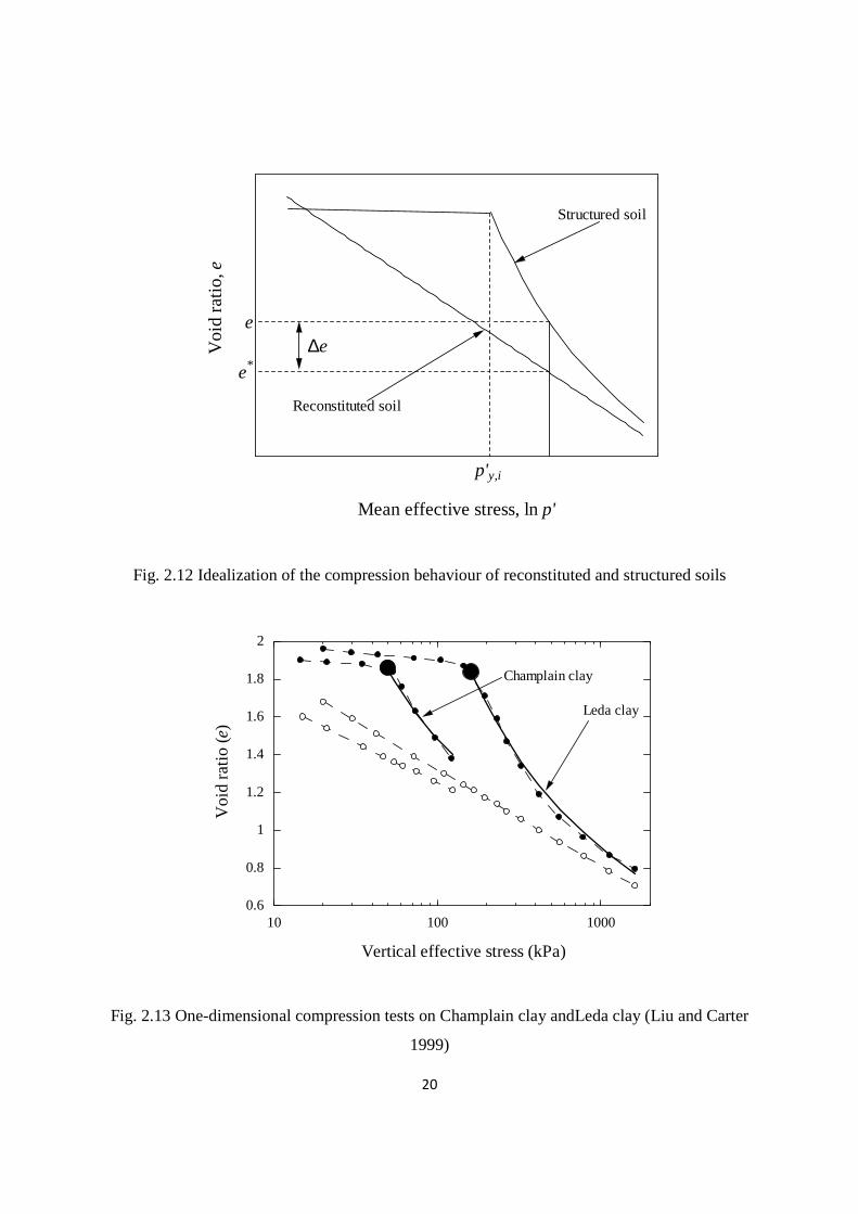
Fig. 2.12 Idealization of the compression behaviour of reconstituted and structured soils .......... 20

Fig. 2.13 One-dimensional compression tests on Champlain clay andLeda clay (Liu and Carter

1999) ................................................................................................................................ 20

x

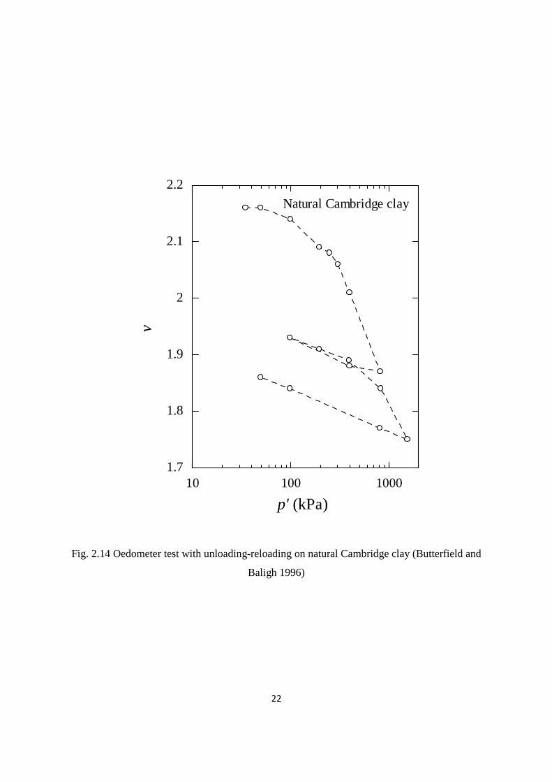
Fig. 2.14 Oedometer test with unloading-reloading on natural Cambridge clay (Butterfield and

Baligh 1996) .................................................................................................................... 22

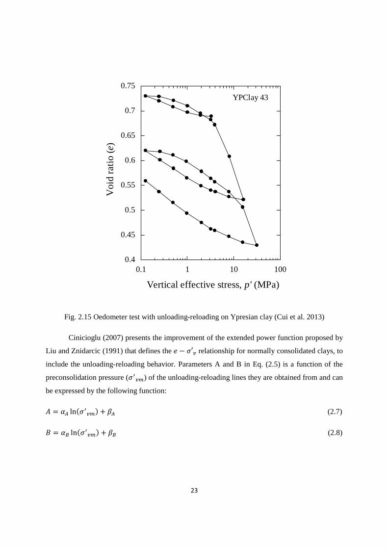
Fig. 2.15 Oedometer test with unloading-reloading on Ypresian clay (Cui et al. 2013) .............. 23

Fig. 2.16 Measured and predicted loading, unloading-reloading paths by Cinicioglu’s model for a

Speswhite kaolinite sample (Cinicioglu 2007) ................................................................ 24

Fig. 2.17 Definition of symbols in log�� versus log�′� plot: (a) single unloading-reloading; (b)

intermediate unloading-reloading .................................................................................... 26

Fig. 2.18 Measured and predicted loading, unloading-reloading paths by Butterfield’s model for

a natural Venetian silty-clay (Butterfield 2011) .............................................................. 27

Fig. 2.19 Relationship between normalized yield stress, ′� ′��⁄ and strain rate (��) (modified

from Watabe et al. 2012) ................................................................................................. 29

Fig. 2.20 Ranges of strain rates encountered in laboratory tests and in situ (Leroueil 2006) ....... 29

Fig. 3.1 Locations of sampling site ............................................................................................... 33

Fig. 3.2 Measured loading and unloading-reloading paths of samples of soft Ariake clay:

(a)′� ′�⁄ = 4; (b) ′� ′�⁄ = 16 ................................................................................. 38

Fig. 3.3 Measured loading and unloading-reloading paths of samples of medium Ariake clay:

(a)′� ′�⁄ = 4; (b) ′� ′�⁄ = 8 .................................................................................... 39

Fig. 3.4 Measured loading and unloading-reloading paths of samples of reconstituted Ariake

clay: (a)′� ′�⁄ = 4; (b) ′� ′�⁄ = 8 ........................................................................... 40

Fig. 3.5 Effect of the value of ′� ′�⁄ on induced plastic deformation of reconstituted Ariake

samples ............................................................................................................................ 41

Fig. 3.6 Measured repeated intermediate unloading-reloading paths of samples of soft Ariake

clay (′� ′�⁄ = 8): (a)′� = ′�; (b) ′� < ′� < ′� ................................................. 42

xi


clay (′� ′�⁄ = 4): (a)′� = ′�; (b) ′� < ′� < ′� ................................................. 43

Fig. 3.8 Measured repeated intermediate unloading-reloading paths of samples of medium

Ariake clay (′� ′�⁄ = 8): (a)′� = ′�; (b) ′� < ′� < ′� ..................................... 44


Ariake clay (′� ′�⁄ = 4): (a)′� = ′�; (b) ′� < ′� < ′� ..................................... 45

Fig. 3.10 Measured repeated intermediate unloading-reloading paths of samples of reconstituted

Ariake clay (′� ′�⁄ = 8): (a)′� = ′�; (b) ′� < ′� < ′� ..................................... 46

Fig. 3.11 Effect of small intermediate reloading-unloading on general unloading path induce

plastic deformation of reconstituted Ariake clay ............................................................ 48

Fig. 3.12 Effect of small intermediate reloading-unloading on general reloading path induce

plastic deformation of reconstituted Ariake clay ............................................................ 49

Fig. 3.13 Effect of number of unloading-reloading cycles (reconstituted Ariake clay samples) . 52

Fig. 3.14 Effect of number of unloading-reloading cycles (soft Ariake clay samples) ................ 53

Fig. 3.15 Effect of time interval between two loading steps on yield stress of undisturbed Ariake

clay .................................................................................................................................. 54

Fig. 4.1 Measured and predicted loading and unloading-reloading paths of samples of medium

Ariake clay: (a)′� ′�⁄ = 4; (b) ′� ′�⁄ = 8 ............................................................... 59

Fig. 4.2 Measured and predicted loading and unloading-reloading paths of samples of soft Ariake

clay: (a)′� ′�⁄ = 4; (b) ′� ′�⁄ = 16 ......................................................................... 60

Fig. 4.3 Measured and predicted loading and unloading-reloading paths of samples of

reconstituted Ariake clay: (a)′� ′�⁄ = 4; (b) ′� ′�⁄ = 8 ......................................... 61

Fig. 4.4 Measured and predicted repeated intermediate unloading-reloading paths of samples of

medium Ariake clay: (a)′� = ′�; (b) ′� < ′�.......................................................... 62

xii


soft Ariake clay (′� ′�⁄ = 4): (a)′� = ′�; (b) ′� < ′� ......................................... 63


soft Ariake clay (′� ′�⁄ = 8): (a)′� = ′�; (b) ′� < ′� ......................................... 64


reconstituted Ariake clay: (a)′� = ′�; (b) ′� < ′� .................................................. 65

Fig. 4.8 Illustration of changing ′� value: (a)�� > ��"; �� < ��" ........................................ 69

Fig. 4.9 Relationship between #′� #′$⁄ and%& ............................................................................ 70

Fig. 4.10 Relationship between #′� #′�⁄ and%& .......................................................................... 70

Fig. 4.11 Measured and predicted intermediate unloading-reloading curves (medium Ariake

clay): (a)′� = ′�; (b) ′� < ′� .................................................................................. 73

Fig. 4.12 Measured and predicted intermediate unloading-reloading curves (reconstitued Ariake

clay): (a)′� = ′�; (b) ′� < ′� .................................................................................. 74

Fig. 4.13 Measured and predicted intermediate unloading-reloading curves (soft Ariake clay)

(′� ′�⁄ = 8): (a)′� = ′�; (b) ′� < ′� ................................................................... 75


(′� ′�⁄ = 4): (a)′� = ′�; (b) ′� < ′� ................................................................... 76

Fig. 4.15 (a) Effect of small intermediate reloading-unloading on general unloading path induce

plastic deformation of reconstituted Ariake clay (b) Simulated results .......................... 77

Fig. 4.16 (a) Effect of small intermediate reloading-unloading on general reloading path induce

plastic deformation of reconstituted Ariake clay (b) Simulated results .......................... 78

Fig. 4.17 Relationship betweenlog�′� ′��⁄ ) and log�� for natural clayey soil ..................... 79

Fig. 5.1 Land-subsidence observation well points in Saga Plain .................................................. 87

xiii

Fig. 5.2 Schematic view of observation points at Ariake well site ............................................... 87

Fig. 5.3 Soil profile and physical and mechanical properties at Ariake well site ......................... 88

Fig. 5.4 Soil profile and physical and mechanical properties at Shiroishi well site ..................... 88

Fig. 5.5 Variations of pore-water pressure in clayey layers at Ariake well site ........................... 90

Fig. 5.6 Variations of pore-water pressure in clayey layers at Shiroishi well site ........................ 91

Fig. 5.7 Compression of soil layers from 0 to 27.2 m depth at Ariake well site .......................... 92

Fig. 5.8 Compression of soil layers from 0 to 22.5 m depth at Shiroishi well site ....................... 92

Fig. 5.9 Location of Yokahama observation site (information from Sugimoto and Akaishi 1986)

......................................................................................................................................... 93

Fig. 5.10 Soil profile and some physical and mechanical properties at Yokohama location

(Sugimoto et al. 1993; Sugimoto and Akaishi 1986) ...................................................... 94

Fig. 5.11 Location of piezometer and settlement gauge at Yokohama site .................................. 95

Fig. 5.12 Measured pore-water pressure at Yokohama site .......................................................... 96

Fig. 5.13 Measured and simulated compressions of clayey soil layers at Yokohama site ........... 99

Fig. 5.14 Difference between the general variation trade and actual pore-water pressure

variations in Saga Plain, Japan ...................................................................................... 100

Fig. 5.15 Measured and simulated pore-water pressure at Yokohama site ................................ 101

Fig. 5.16 Comparison of measured and simulated compressions of clayey soil layers at

Yokohama site ............................................................................................................... 102

Fig. 5.17 Soil profile and some physical and mechanical properties at Romaneenart Park site

(Seven Associated Consultants Co., Ltd. 2012) ............................................................ 105

xiv

Fig. 5.18 Soil profile and some physical and mechanical properties at Kasetsart university

campus site (Seven Associated Consultants Co., Ltd. 2012) ........................................ 105

Fig. 5.19 Location of piezometer and settlement gauge at Kasetsart University campus site .... 106

Fig. 5.20 Simulated and measured pore-water pressure variations at Romaneenart Park site ... 108

Fig. 5.21 Simulated and measured pore-water pressure variations at Kasetsart University campus

site ................................................................................................................................. 109

Fig. 5.22 Measured and simulated compressions of clayey soil layers at Romaneenart Park site

....................................................................................................................................... 110

Fig. 5.23 Measured and simulated compressions of clayey soil layers at Kasetsart University

campus site .................................................................................................................... 110

xv

LIST OF TABLES

Table 3.1 Single unloading-reloading testsTable .......................................................................... 34

Table 3.2 Repeated unloading-reloading tests .............................................................................. 35

Table 3.3 Small intermediate unloading-reloading test ................................................................ 36

Table 4.1 Values of model parameter for medium, soft and reconstituted Ariake clay

samplesTable ................................................................................................................ 57

Table 4.2 Values of#′�,#′$and #′�for simulating repeated intermediate unloading-reloading

cycles for medium, soft and reconstituted Ariake clay samples .................................. 58

Table 4.3 Values of#′� and#′$ for simulating small intermediate unloading-reloading cycles for

reconstituted Ariake clay samples ................................................................................ 72

Table 5.1 Initial conditions and parameters used in analysis for Ariake and Shiroishi sites ........ 89

Table 5.2 Initial conditions and parameters used in analysis for Yokohama site ......................... 97

Table 5.3 Initial conditions and parameters used in analysis for Romneenart Park site ............ 106

Table 5.4 Initial conditions and parameters used in analysis for Kasetsart University campus site

.................................................................................................................................... 107

xvii

LIST OF NOTATIONS

' dimensionless parameter

( dimensionless parameter

#� compression index

#$ swelling index

#′� slope of the virgin loading line in log�� − log�� plot

#′� slope of intermediate unloading line in log�� − log�� plot

#′� slope of the tangent to the reloading curve at = ′� in log�� − log�� plot

#′�" slope of the tangent to the reloading curve at = ′�" in log�� − log�� plot

#) initial slope of the reloading curve in log�� − log�� plot

#′$ slope of the first unloading line in log�� − log�� plot

� void ratio

�∗ corresponding voids ratio for the reconstituted soil

�� soil parameter

�� initial void ratio

∆� component due to the structure

, hydraulic head

-�. hydraulic conductivity of lower layer

-�/ hydraulic conductivity of upper layer

0� coefficient of volume compressibility

1#& overconsolidation ratio

′ vertical effective stress

′ current mean effective stress

′� vertical effective stress

′�" new value of ′�

′� vertical effective stress at the end of unloading

′�" vertical effective stress at the end of intermediate unloading

′� reloading pressure where the reloading line merges with the virgin curve

′� intermediate unloading pressure

xviii

′� consolidation yield stress

′�2 Lower limit of ′�

′�� yield stress corresponding to a strain rate of 1045�64 � ′7,9 mean effective stress at which virgin yielding of the structured soil begins

: 4; dimensionless stiffness coefficient for one-dimensional strain

<9 field initial pore-water pressure

� specific volume

�� specific volume corresponding to ′� on the reloading line

�� volume at previously unloading curve corresponding to the vertical effective

stress ′�"

��" specific volume at the start of current reloading curve with a vertical effective

stress of ′�"

=> natural water content

? Additional soil parameter having a unit of stress

@A dimensionless parameter

@B dimensionless parameter

CA dimensionless parameter

CB dimensionless parameter

�� field strain rate

�� strain rate of standard oedometer test

�� strain rate

DE total unit weight

DF unit weight of water

G total stress

G′ effective stress

G′� vertical effective stress

G′�9 field initial vertical effective stress

G′�H Preconsolidation stress

G7 yielding vertical effective stress

G7� yielding vertical effective stress from laboratory oedometer test

CHAPTER 1

INTRODUCTION

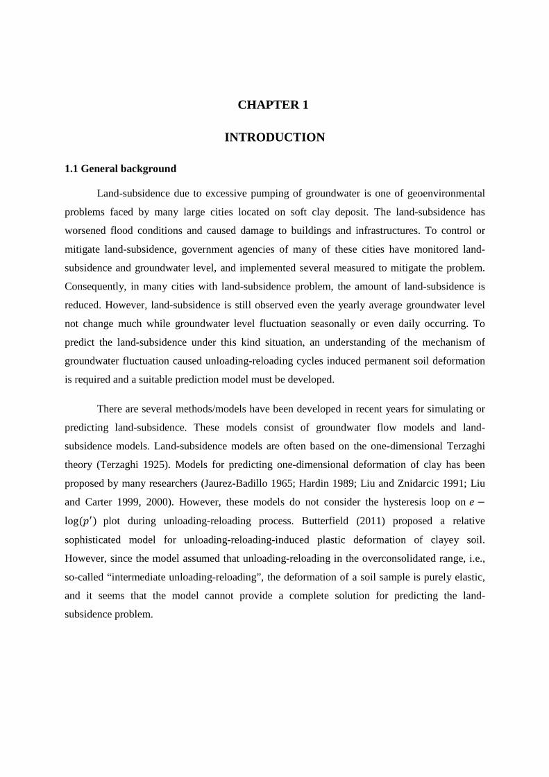
1.1 General background

Land-subsidence due to excessive pumping of groundwater is one of geoenvironmental

problems faced by many large cities located on soft clay deposit. The land-subsidence has

worsened flood conditions and caused damage to buildings and infrastructures. To control or

mitigate land-subsidence, government agencies of many of these cities have monitored land-

subsidence and groundwater level, and implemented several measured to mitigate the problem.

Consequently, in many cities with land-subsidence problem, the amount of land-subsidence is

reduced. However, land-subsidence is still observed even the yearly average groundwater level

not change much while groundwater level fluctuation seasonally or even daily occurring. To

predict the land-subsidence under this kind situation, an understanding of the mechanism of

groundwater fluctuation caused unloading-reloading cycles induced permanent soil deformation

is required and a suitable prediction model must be developed.

There are several methods/models have been developed in recent years for simulating or

predicting land-subsidence. These models consist of groundwater flow models and land-

subsidence models. Land-subsidence models are often based on the one-dimensional Terzaghi

theory (Terzaghi 1925). Models for predicting one-dimensional deformation of clay has been

proposed by many researchers (Jaurez-Badillo 1965; Hardin 1989; Liu and Znidarcic 1991; Liu

and Carter 1999, 2000). However, these models do not consider the hysteresis loop on � −log�� plot during unloading-reloading process. Butterfield (2011) proposed a relative

sophisticated model for unloading-reloading-induced plastic deformation of clayey soil.

However, since the model assumed that unloading-reloading in the overconsolidated range, i.e.,

so-called “intermediate unloading-reloading”, the deformation of a soil sample is purely elastic,

and it seems that the model cannot provide a complete solution for predicting the land-

subsidence problem.

2

1.2 Objective and scopes of study

The objective of this study is to develop a method/model for simulating the land-

subsidence due to daily fluctuations of pore-water pressure of clayey soil deposit. To understand

the mechanism of daily fluctuations of pore-water pressure induced land-subsidence, the

laboratory oedometer tests will be carried out to investigate the deformation behaviour of clay

induced by repeated intermediate unloading-reloading cycles. Then, a suitable prediction model

for predicting the deformation of soil sample will be developed based on the results of laboratory

test. Finally, the proposed model will be applied to simulate ground deformation induced by

groundwater fluctuations for five (5) field case histories.

1.3 Organization of this study

This dissertation contains six chapters. Firstly, the introduction (Chapter 1) describes the

general background and objective and scopes of the study. Chapter 2 reviews the literature about

land-subsidence, unloading-reloading effect on one-dimensional deformation behaviour and

strain rate effect on consolidation yield stress (′�). Chapter 3 describes relevant details of the

experimental investigations carried out in this study and presents the deformation behaviour of

Ariake clay based on oedometer test results. Chapter 4 presents the proposed unloading-

reloading model to simulate the laboratory test results. Chapter 5 presents the applications of

proposed model to field case histories. Finally, the conclusions drawn from this study and

recommendations for future works are given in Chapter 6.

CHAPTER 2

LITERATURE REVIEW

2.1 Land-subsidence

Land-subsidence is a geoenvironmental phenomenon, in which the ground surface goes

down due to ground compression. There are many causes of land-subsidence, including fluid

withdrawal, oil and gas and groundwater pumping, mining operations, natural settlement, hydro-

compaction, settlement of collapsible soils, settlement of organic soils and sinkholes (Budhu and

Adiyaman 2010). The primary reason for land-subsidence of many cities around the world where

located on soft clay deposits is pumping of groundwater. Land-subsidence due to excessive

pumping of groundwater causes many problems, including damage to structures (buildings,

roads and highways, railroads, flood-control structures, well-casings, gas and water pipes,

transmission lines, electric and gas substations, and sewer lines), flow reversal in drains, canals,

irrigation systems and aquifers.

In the Choshui River alluvial fan area, Taiwan, due to excessive pumping of groundwater

resulted in both groundwater drawdown and severe land subsidence, especially during 1950s–

1990s (Liu et al. 2004).

In Bangkok Plain, Thailand, aquifer system consists of 8 main aquifers (Giao et al. 2012).

The upper four aquifers in 200 m deep zone are the Bangkok (BK) aquifer (~50 m depth); the

Phra Pradaeng (PD) aquifer (~100 m depth); Nakorn Laung (NL) aquifer (~150 m depth) and

Nonthaburi (NB) aquifer (~200 m depth). The yearly groundwater usage is shown in Fig. 2.1.

Fig. 2.2 shows land-subsidence and piezometric drawdowns of Bangkok aquifer versus time

(Phien-wej et al. 2006). From Figs 2.1 and 2.2, it can be seen that there is a strong correlation

between amount of groundwater pumped, the groundwater level, and the rate of land-subsidence.

Groundwater over-pumping led to drastic drawdown in piezometric head and land-subsidence

has become widely evident in Bangkok area.

4

Fig. 2.1 Groundwater pumping from the Bangkok Aquifer (Phien-wej et al. 2006)

In order to control or mitigate this land-subsidence, groundwater pumping has been

strictly regulated or controlled in these cities. Consequently, in these cities with land-subsidence

problems, there has been no further excessive groundwater drawdown, or even certain recovering

in term of the average groundwater level. For examples, in Bangkok Plain, Thailand, as a result

of several measures to regulate and reduce groundwater use, the groundwater level was

recovered since 1997. However, the monitored data in Fig. 2.3 shows that land-subsidence still

occurred while groundwater levels increase (Fornes and Pirarai 2014). It is well known that land-

subsidence due to excessive pumping of groundwater occurs as a result of consolidation with an

increase in effective stress of the clay layer adjacent to the pumped aquifer due to decreased

pore-water pressure from groundwater withdrawal. However, land-subsidence dependent not

only on increase in effective stress in the clayey layer but also on the cyclic effect of

consolidation of the clayey layer due to seasonal fluctuations in groundwater level (Sakai 2001).

When water is added (natural and artificial recharge) to the soil mass and groundwater level rises,

the effective stress on the soils are reduced causing ground uplift. However, soils are not elastic

material, hence; land-subsidence/uplift is not directly proportional to the amount of groundwater

0

0.2

0.4

0.6

0.8

1

1.2

1.4

1.6

1.8

2

2.2

2.4

2.6

Year

Gro

undw

ate

r us

ag

e (

mill

ion

cu.

m/d

ay)

1955 1960 1965 1970 1975 1980 1985 1990 1995 2000 2005

5

withdrawal/recharge. In addition, the amount of uplift is not equal to the amount of land-

subsidence for normally consolidated soils for a similar change in absolute groundwater level.

Fig.2.2 Land-subsidence and piezometric drawdowns of Bangkok aquifers versus time (Phien-

wej et al. 2006); (a) Southeastern location (b) Southwestern location

20

30

40

50

60

70

Year

De

pth

of p

iezo

me

tric

leve

lb

elo

w g

roun

d s

urf

ace

(m

)

1978 1980 1982 1984 1986 1988 1990 1992 1994 1996 1998

PD (112m)

NL (156m)

La

nd

-su

bsi

de

nce

fro

m 1

97

8 (m

m)0

50

100

150

200

250

300

350

400

450

500

Settlement (1m)

NB (207m)a) Bang Pli, Southeastern Bangkok

0

10

20

30

40

50

60

70

80

Year

De

pth

of p

iezo

me

tric

leve

lbe

low

gro

und

surf

ace

(m

)

1978 1980 1982 1984 1986 1988 1990 1992 1994 1996 1998

PD (102m)

NB (207m)

La

nd-s

ubsi

denc

e f

rom

197

8 (m

m)-20

020406080

100120140160180200220240260280300

Settlement (1m)

NL (169m)

b) Samut Sakorn, Southwestern Bangkok

6

In Changzhou, China, excessive groundwater withdrawal has caused severe land-

subsidence (Zhang et al. 2010). The Quaternary deposits of this area are composed of five

aquifers: one unconfined and/or semi-confined aquifer and four confined aquifers. The second

confined aquifer is the main exploited aquifer. The groundwater in the third aquifer flowed

upward to the second confined aquifer and the groundwater in it is affected by that in the second

confined aquifer. The extraction of groundwater in this area began in 1927 and the extensive

extraction of groundwater occurred after 1983 when the town industries developed rapidly. The

changes in groundwater level and compression in the second and third confined aquifers are

shown in Fig. 2.4. Due to decreasing of groundwater pumping, the groundwater level in the

second confined aquifer reached its lowest value in 1994 and then rose up. However,

compression was still measured. The groundwater level in the third confined aquifer began to

recover and rose from the lowest value in 2000. It can be also seen that land-subsidence still

occurred during recovery of groundwater level.

In Saga Plain, Japan, it is commonly divided into two districts; the Saga district and the

Shiroishi district. Groundwater levels and land-subsidence are shown in Fig. 2.5 (Sakai 2001). In

the Saga district, pumping of groundwater, mainly for industrail use, has decreased significantly

from 1970’s due to regulations by Saga Prefecture in 1974. Fig. 2.5(a) shows measured

groundwater level and land-subsidence at observation well in Saga district. The groundwater

level appears to have recovered. However, it can be clearly seen that land-subsidence occured

even during the recovery of groundwater level. In the Shiroishi district, groundwater extraction,

mainly for agriculture and residential supply, has increased due to land reclamation and the

limited extent of irrigation by surface flow. The measured land-subsidence at observation well in

Shiroishi district has continued irreversibly due to the periodic change in groundwater level,

which is depressed in summer and then recharged to almost original levels in winter as shown in

Fig. 2.5(b). Rapid land-subsidence was observed during the daught as a result of the severe

depletion of the aquifer due to the extreme pumping of groundwater.

Sakai (2001) reported measured groundwater level and land-subsidence at the new

observation well where located in the Shiroishi district. The measuring time interval was 1 hour.

The monitored data indicate that the groundwater level sometimes varied daily as shown in Fig.

2.6(a). There are small fluctuations of the groundwater level superposed on both a general trend

7

of drawdown and recovery of the groundwater level. The magnitude of these fluctuations may be

only a few centimeters and there was monitored land-subsidence under this kind of situation as

shown in Fig. 2.6(b). There is a question that does this kind of small fluctuations can induce

land-subsidence? Since the permanent deformation induced by unloading-reloading cycles in

overconsolidated range is relatively small, it has not been comprehensively investigated, and as a

result, there is very limited published data in the literature. However, considering land-

subsidence problem, this issue has an important practical impact because there are many cases

where generally groundwater was in a recovering tendency, but there were observed increment

of land-subsidence. Therefore, providing a general understanding of the effect of small

reloading-unloading (or unloading-reloading) process on permanent deformation of clayey soil

has both theoretical and practical significance. In order to predict the ground deformation due to

such fluctuations, an understanding of the effect of small reloading-unloading (or unloading-

reloading) cycles on permanent deformation of clayey soil is required, and a suitable prediction

model must be developed.

Fig. 2.3 Water level from three major aquifers and total land-subsidence in Central Bangkok

(Fornes and Pirarai 2014)

15

20

25

30

35

40

45

50

55

60

Year

Sta

tic w

ate

r le

vel (

m)

1978 1982 1986 1990 20021994 20061998

PD (100m)

NL (150m)

Tot

al l

an

d-su

bsid

enc

e (

cm)

-80

-70

-60

-50

-40

-30

-20

-10

0

10

Land subsidence NB (200m)

8

Fig. 2.4 Changes of groundwater level and compression of confined aquifer in Changzhou, China

(Zhang et al. 2010); a) the second confined aquifer b) the third confined aquifer

30

40

50

60

70

80

90

Year

Com

pres

sion

(m

m)

1990 1994 2002 20061998

groundwater level

Gro

und

wat

er le

vel (

m)

-80

-75

-70

-65

-60

-55

-50

compression

a)

0

40

80

120

160

Year

Com

pres

sio

n (m

m)

1990 1994 2002 20061998

groundwater level

Gro

und

wat

er le

vel (

m)

-68

-64

-60

-56

-52

compression

b)

9

Fig. 2.5 Fluctuation of groundwater level and subsidence at observation wells in Saga Plain,

Japan (modified from Sakai 2001)

-25

-20

-15

-10

-5

0

Sub

side

nce

(cm

)

Gro

un

dw

ater

leve

l (m

)

Saga (depth: 197 m)

：subsidence

：groundwater level

30

0

-10

-20

(a)

-40

-35

-30

-25

-20

-15

-10

-5

0

Sub

side

nce

(cm

)

1975 '76 '77 '78 '79 '80 '81 '82 '83 '84 '85 '86 '87 '88 '89 '90 '91 '92 '93 '94 '95 '96 '96 '98 '99

Shiroishi (depth: 260 m)

Gro

un

dw

ater

leve

l (m

)

0

-10

-20

10

20

-30

-40

-50

-60

-70

10

20 (b)

10

Fig. 2.6 Daily fluctuation of groundwater level in clayey soil deposit and subsidence at new

observation wells in Saga Plain, Japan (modified from Sakai 2001)

-4

-3

-2

-1

0

6/1 9/1 12/1 3/1 6/11996 1997

Gro

undw

ater

leve

l (T

.P:ｍ

)

(a)

G.L.-21.0 m

-30

-20

-10

0

Sub

side

nce

(mm

) G.L.-27.2m

New Ariake Observation Well

(b)

Year

11

2.2 Mechanism of consolidation cause by pore-water pressure drawdown in an aquifer

Various approaches have been developed for analyzing and modeling land-subsidence

follow from the basic relations between head, stress, compressibility, and groundwater flow. To

predict land-subsidence due to pumping of groundwater, two models are required: 1) a seepage

flow model; 2) a subsidence model. The pumping of groundwater induced compression of soil

layers is a three-dimensional (3D) problem. However, to conduct 3D analysis, it is difficult to

define a proper hydraulic boundary condition. For some observation points, groundwater level in

aquifer or even the pore-water pressure in clayey layer, and the compression of each layer were

monitored (e.g. Sakia 2001; Seven Associated Consultants Co., Ltd. 2012). A one-dimensional

(1D) analysis can be conducted by specifying the water level in each aquifer and simulating the

consolidation process. Then the interaction between aquifers and the distribution of pore-water

pressure can be analyzed with a verified numerical procedure and parameters. The principle of

effective stress, proposed by Karl Terzaghi in 1925, is often used to explain the occurrence of

land-subsidence related to groundwater withdrawal (Galloway et al. 1999). Base on the effective

stress concept (Terzaghi 1925), the total stress, effective stress, and hydraulic head can be

expressed as follows:

G = G − DF, (2.1)

where G is the effective stress; G is the total stress; DF is the unit weight of water; , is the

hydraulic head. Base on Terzaghi’s 1-D consolidation theory, during with drawdown and/or

recovery of groundwater level, total vertical stress is constant and G will change with the

hydraulic head as follows:

IG = −DFI, (2.2)

The relationship between the stress increment and the strain increment can be expressed by

following function:

I� = −0�IG′ (2.3)

where 0� is the coefficient of volume compressibility of the soil. By this principle, pumping of

groundwater will induce an increase in effective stress of the clayey layers adjacent to the

12

pumped aquifer due to decreased pore-water pressure from excessive groundwater withdrawal.

Because compression of clayey soil is controlled by effective stress, the increase of effective

stress will cause decrease of pore volume and when the compression is transferred to the ground

surface and resulted in land-subsidence.

Chai et al. (2004) discussed the mechanism of consolidation caused by pore-water

pressure drawdown in aquifer. The phreatic level does not change much, which corresponds to a

zero excess pore-water pressure boundary at the ground surface, and the final state is a

drawdown steady flow from the ground surface to the aquifer. For a given amount of

groundwater level drawdown in the aquifer, the relative values of hydraulic conductivity of clay

layer above the aquifer play an important role on amount of settlement. For the several field

measurements, the pattern of pore-water pressure distribution within the clay layers, where is

above an aquifer, is a leftward concave distribution with the condition the value of hydraulic

conductivity of upper layer is higher than that of the lower layer (-�/ > -�.) as shown in Fig.

2.7.

Fig. 2.7 A possible pore-water pressure drawdown pattern (Chai et al. 2004)

13

For settlement analysis, consolidation analysis can incorporate many constitutive models

to consider the elastic, elastoplastic, and creep behaviour of soft soil. Budhu and Adiyaman

(2013) used a modified Cam-clay model (Roscoe and Burland 1968) to describe the elasto-

plastic deformation characteristics of aquitards. Chai et al. (2005) considered the land-subsidence

in Shanghai due to groundwater level drawdown and predicted future land-subsidence by

assuming the several drawdown scenarios. In the analysis, 1-D consolidation analysis was

conducted, in which soft clay in the aquitards was simulated by modified Cam-clay model. The

calculated results were compared with the field measured data; the results show that the

predicted results can simulated the field measured values well. However, clay often has creep

property, that deformation of clay is time-dependent even when the effective stress in it remains

a constant. Corapcioglu and Brutsaert (1977) applied the Merchant’s visco-elastic model

(Merchant 1939) to simulate land-subsidence. Ye et al. (2012) employed the modified

Merchant’s model to calculate the compaction of aquitard and aquifer in Shanghai and concluded

that it was better than elasto-plastic models in land-subsidence simulation. Zhang et al. (2015)

developed a fully coupled visco-elasto-plastic model that can make the groundwater flow and

compression of aquitard fully coupled, and can describe various deformation characteristics of

aquitards under long-term groundwater withdrawal. However, the test results from Zhang et al.

(2011) show that under cycles of unloading-reloading the creep deformation can be neglected

from the third cycle of unloading-reloading.

Although the existing seepage flow and consolidation model can simulate soil

deformation and mechanism of land-subsidence due to groundwater withdrawal in a certain

range, these models cannot explain the phenomenon of land-subsidence increasing continuously

without groundwater withdrawal. Some researchers considered that underground structures may

change the groundwater environment (Xu et al. 2012a; Wu et al. 2015). Underground structures

which constructed below the water table will obstruct groundwater flow in term of velocity and

direction. Xu et al. (2012b) concluded that the average land-subsidence in the urban area in

Shanghai is related to the comprehensive effect of large number of underground structures. The

average rate of land-subsidence increases with the increase of ratio of the volume of underground

structure to the volume of aquifer. Generally, groundwater flows from a position with a high

potential to a position with a low potential. When groundwater is pumped into the urban centre,

the groundwater can be recharged from the suburban area. However, the cut-off effect on

14

groundwater flow due to the existence of underground structures in aquifers causes continuous

reductions in groundwater level in aquifer in the urban centre (Xu et al. 2012a). In some

excavation cases, a cut-off wall is not deep enough to cut off the groundwater and therefore

dewatering usually continues for several months or even more than a year. This long-term

dewatering causes the reduction of groundwater level during an extended period of time, which

may cause settlement of surrounding ground (Shen et al. 2014).

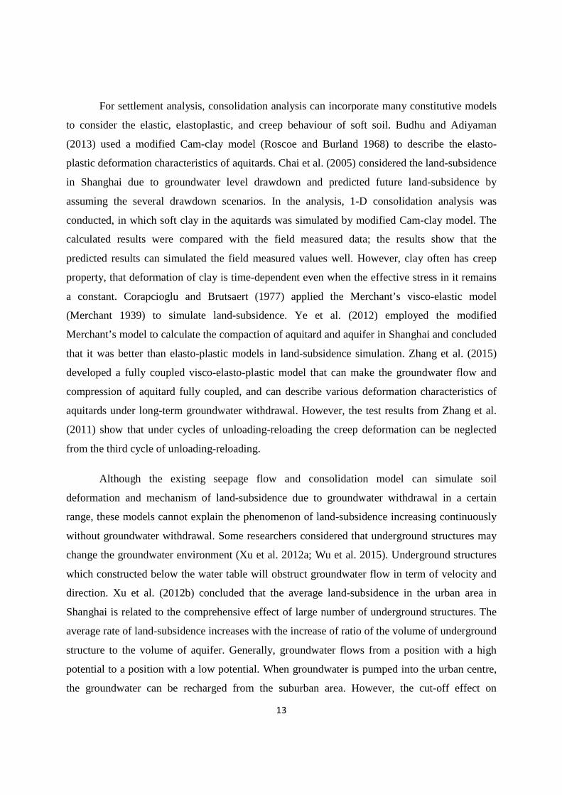
2.3 Unloading-reloading effect on one-dimensional deformation behaviour

Deformation behavior of soil deposits has been studied throughout the history of soil

mechanics since Terzaghi first described the oedometer test in 1925. Typically, the deformation

characteristics are usually presented by plotting a logarithm of vertical effective stress (’) against void ratio (�) as shown in Fig. 2.8. When expressed in this way, the characteristic has

been divided into two regions; a linear elastic curve (recompression or swelling curve) at low

stress and a linear virgin compression curve at higher stress. The slope of the virgin compression

curve and the linear elastic curve are commonly called the compression index (#� ) and the

swelling index (#$), respectively. The transition point between the linear elastic curve and the

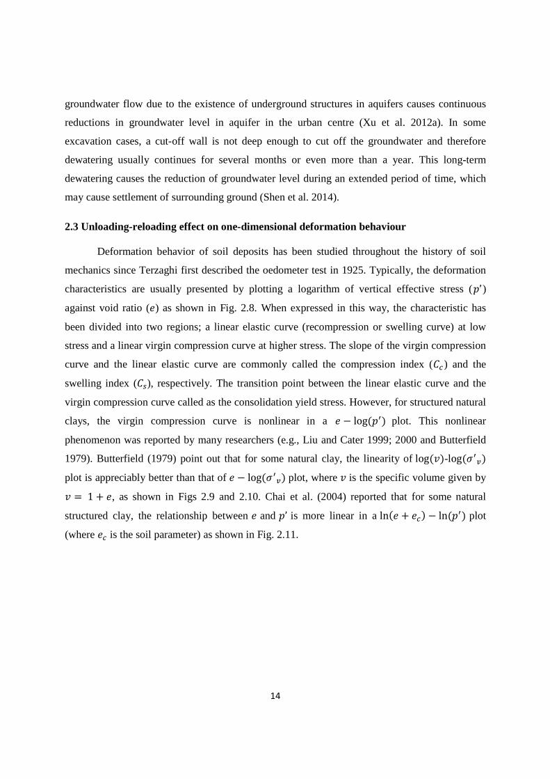
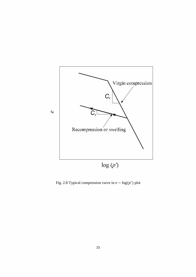
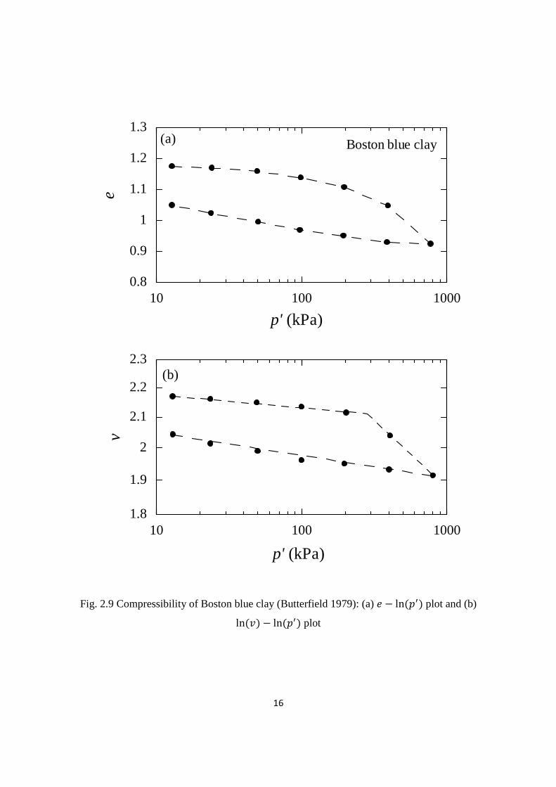
virgin compression curve called as the consolidation yield stress. However, for structured natural

clays, the virgin compression curve is nonlinear in a � − log�� plot. This nonlinear

phenomenon was reported by many researchers (e.g., Liu and Cater 1999; 2000 and Butterfield

1979). Butterfield (1979) point out that for some natural clay, the linearity of log��-log�G�� plot is appreciably better than that of � − log�G�� plot, where � is the specific volume given by

� = 1 + �, as shown in Figs 2.9 and 2.10. Chai et al. (2004) reported that for some natural

structured clay, the relationship between � and ’ is more linear in aln�� + �� − ln�� plot

(where �� is the soil parameter) as shown in Fig. 2.11.

15

Fig. 2.8 Typical compression curve in � − log�� plot

16

Fig. 2.9 Compressibility of Boston blue clay (Butterfield 1979): (a) � − ln�� plot and (b)

ln�� − ln�� plot

10 100 10000.8

0.9

1

1.1

1.2

1.3

p' (kPa)

e

Boston blue clay

(b)

10 100 10001.8

1.9

2

2.1

2.2

2.3

v

p' (kPa)

(a)

17

Fig. 2.10 Compressibility of Chicago clay (Butterfield 1979): (a) � − ln�� plot and (b)

ln�� − ln�� plot

10 100 10000.6

0.8

1

1.2

1.4

1.6

p' (kPa)

e

Chicago clay

10 100 10001.6

1.8

2

2.2

2.4

2.6

v

p' (kPa)

(a)

(b)

18

Fig. 2.11 Compression curve for Leda clay (Chai et al. 1979): (a) � − ln�� plot and (b)

ln�� + �� − ln�� plot

10 100 10000.5

1

1.5

2

p' (kPa)

e

Leda clay

e - ln(p')

(b)

10 100 10000.2

0.4

1

2

e -

0.7

p' (kPa)

ln(e-0.7) - ln(p')

(a)

19

Various forms of mathematical functions, ranging in complexity from constant values for

compressibility to logarithmic, exponential, and power function, have been proposed by many

researchers.

Hardin (1989) proposed a1/� versusG′� model for one-dimensional deformation as

follows:

L =

LM + NOPQ RSTUV W

� (2.4)

where 1/�� = intercept at G′� = 0, and the reciprocal slope : 4; is the dimensionless stiffness

coefficient for one-dimensional strain.

Liu and Znidarcic (1991) proposed an extended power-function model. It is expressed by

following function:

� = '�G + ?�B (2.5)

in which A and B are constants and Z is an additional soil parameter having a unit of stress. The

model parameters are obtained by least-square fitting to the experimental data.

Liu and Carter (1999) proposed a model for virgin compression of structured soils. An

illustration of a material idealization the compression behaviour of structured soils is shown in

Fig. 2.12. The void ratio for structured soil, �, can be expressed by following function:

� = �∗ + ∆� for ′ ≥ ′7,9 (2.6)

where �∗ is the corresponding voids ratio for the reconstituted soil, ∆� is the component due to

the structure, is the current mean effective stress, and ′7,9 is the mean effective stress at

which virgin yielding of the structured soil begins. Comparisons between the theoretical equation

and the experimental data of Champlian clay and Lada clay are shown in Fig. 2.13.

20

Fig. 2.12 Idealization of the compression behaviour of reconstituted and structured soils

Fig. 2.13 One-dimensional compression tests on Champlain clay andLeda clay (Liu and Carter

1999)

Mean effective stress, ln p'

Vo

id r

atio

, eStructured soil

Reconstituted soil

p'y,i

e

e*∆e

10 100 10000.6

0.8

1

1.2

1.4

1.6

1.8

2

Vertical effective stress (kPa)

Vo

id r

atio

(e)

Champlain clay

Leda clay

21

However, it is well known that soil compression curves show unloading-reloading loops.

When investigating the compressibility of a soil, unloading-reloading loops are often ignored an

average slope is usually considered in the calculation of soil deformation. This practice is

relatively easy for sandy soils and silty soils, but difficult for clayey soils. Butterfield and Baligh

(1996) reported the oedometer test results with unloading-reloading cycle on many natural and

remolded clays (e.g., natural Drammen clay, natural Cambridge clay and remolded London clay).

Fig. 2.14 shows the oedometer test result with unloading-reloading loop of natural Cambridge

clay. Cui et al. (2013) reported the oedometer test results with several unloading-reloading cycles

on natural stiff clays, Ypresian clays (YPClay), from different depths. Fig. 2.15 shows oedometer

test result with unloading-reloading loops of YPClay at the depth from 330.14 m to 330.23 m.

Yin and Tong (2011) reported the experimental data from oedometer test and proposed a one-

dimensional elastic visco-plastic model considering both for saturated soils exhibiting both creep

and swelling. They believe that the swelling and creep contribute to the formation of unloading-

reloading loop. When a sample is unloaded to the stress-strain state far from the normal

consolidation line, the swelling potential has caused the clay to expand and time dependent

reduction of strain. When the sample is reloaded to the stress-strain state closer to the normal

consolidation line, the sample will have a creep compression.

22

Fig. 2.14 Oedometer test with unloading-reloading on natural Cambridge clay (Butterfield and

Baligh 1996)

10 100 10001.7

1.8

1.9

2

2.1

2.2

p' (kPa)

v

Natural Cambridge clay

23

Fig. 2.15 Oedometer test with unloading-reloading on Ypresian clay (Cui et al. 2013)

Cinicioglu (2007) presents the improvement of the extended power function proposed by

Liu and Znidarcic (1991) that defines the � − G′� relationship for normally consolidated clays, to

include the unloading-reloading behavior. Parameters A and B in Eq. (2.5) is a function of the

preconsolidation pressure (G�H) of the unloading-reloading lines they are obtained from and can

be expressed by the following function:

' = @A ln�G�H� + CA (2.7)

( = @B ln�G�H� + CB (2.8)

0.1 1 10 1000.4

0.45

0.5

0.55

0.6

0.65

0.7

0.75

Vertical effective stress, p' (MPa)

Vo

id r

atio

(e)

YPClay 43

24

where@A , @B , CA and CB are obtained from the semi-logarithmic relationship between the

preconsolidation pressure and the parameters A and B. The � − G′� function can be expressed as

follows:

� = �@Aln�G′�H� + CA�[G� + ?]�[\]^�ST_�`a\� (2.9)

The value of ? is dependent on the form of the respective normally consolidation or unloading-

reloading line, is obtained by a guess and check test. The parameter ? has a single value for

reloading lines and a different single value for unloading lines. Measured and predicted loading,

unloading-reloading paths by Cinicioglu’s model for a Speswhite kaolinite sample are shown in

Fig. 2.16

Fig. 2.16 Measured and predicted loading, unloading-reloading paths by Cinicioglu’s model for a

Speswhite kaolinite sample (Cinicioglu 2007)

Butterfield (2011) proposed a relatively sophisticated model for unloading-reloading-

induced plastic deformation of clayey soil. The basic assumptions adopted are as follows.

0.1 1 10 100 10001.2

1.4

1.6

1.8

2

Vertical effective stress, p' (kPa)

Vo

id r

atio

(e)

Measured Predicted

25

(1) The virgin compression and the unloading lines are linear in a log�� − log�� plot, where

′ is the consolidation pressure (vertical effective stress) and � is the specific volume given by

� = 1 + � (where � is the void ratio). In this plot the slope of the virgin loading line is denoted

as #′� and that of the unloading line is #′$, as shown in Fig. 2.17(a).

(2) For reloading, the log�� − log�� relationship is non-linear, as illustrated in Fig. 2.17(a)

and can be expressed by the following exponential function:

�/�� = bc dR efg[` W h1 − i �f�fjk

[` lm (2.10)

�@ + 1� = log RefnefgW /logi�fV�fjk (2.11)

where ′�is the maximum vertical effective stress before initial unloading, ′� is the vertical

effective stress at the end of unloading, #′) is the initial slope of the reloading curve, #′� is the

slope of the tangent line to the reloading curve at = ′� and �� is the specific volume

corresponding to ′�.

(3) When unloading-reloading on the first reloading line, or so called intermediate unloading-

reloading, the log�� − log�� relationship is linear and the deformation is elastic (recoverable)

with a slope of #′� (#′) < #′� < #′$ ) as also shown in Fig. 2.17(b). Assuming #′� varies

linearly with log�� between the values #′) and #′$, provides:

logReofegfW /logRepf

egfW = log i�of�jfk /log i�qf�jfk (2.12)

where ′� is the reloading pressure where the reloading line merges with the virgin loading curve

and ′� is the intermediate unloading pressure.

Butterfield’s model requires specification of five parameters, viz., #′�, #′$, #′), #′� and

#′� . Fig. 2.18 shows a comparison between measured and predicted loading, unloading-

reloading paths by Butterfield’s model for a natural Venetian silty-clay (Butterfield 2011). It can

be seen that the model can predict the cycle of unloading-reloading well. However, the

assumption that intermediate unloading-reloading will not cause any plastic (irrecoverable)

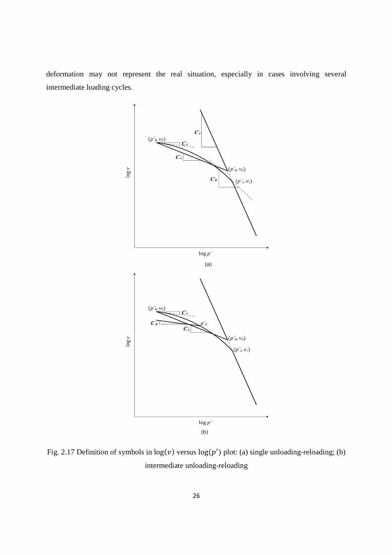
26

deformation may not represent the real situation, especially in cases involving several

intermediate loading cycles.

Fig. 2.17 Definition of symbols in log�� versus log�� plot: (a) single unloading-reloading; (b)

intermediate unloading-reloading

27

Fig. 2.18 Measured and predicted loading, unloading-reloading paths by Butterfield’s model for

a natural Venetian silty-clay (Butterfield 2011)

2.4 Strain rate effect on consolidation yield stress (r′r)

Tanaka et al. (2000) reported the strain rate effect on consolidation yield stress (′�) for

nine undisturbed marine clay deposits obtained from various countries. It was found that the

consolidation yield stress (′�) increase with strain rate. Graham et al. (1983) reported laboratory

0.01 0.05 0.1 0.5 1 5 10 501.3

1.4

1.5

1.6

1.7

1.8

p' (MPa)

v

Venetian silty-clay

C'c= 0.069C's= 0.010C'r= 0.003C'0= 0.039

Test data Fitted model

28

tests on a wide variety of lightly overconsolidated natural clays. The results showed that

important engineering properties such as undrained strength and preconsolidation pressure are

time-dependent. Both the compressibility and the undrained shear strength of naturally cemented

heavily overconsolidated clay were found to be controlled by the time effects (Vaid et al. 1979).

Numerous of constant rate of strain consolidation CRS test were performed to investigate the

effects of strain rate on stress-strain curve of clays and consolidation yield stress. CRS tests using

slow rates of strain resulted in large reductions in apparent preconsolidation pressure and

increased compressibility. Watabe et al. (2008) proposed a simplified method for predicting the

relationship between the consolidation yield stress and the strain rate. The consolidation yield

stresses for different strain rate were obtained from CRS test and long-term consolidation test

(LT test), respectively. The relationship between the consolidation yield stress and the strain rate

is expressed by three isotache parameter (′�2, s and st). The model equation of the strain rate

dependency used in ′� - �� relationship, is as follows.

ln��fu4�fuv�fuv � = s + stln�� (2.13)

where,s and st are constants and ′�2 is the lower limit of ′�.

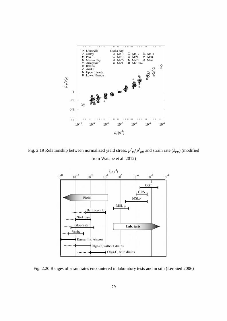
Watabe et al. (2012) summarized the relationship between strain rate (�� ) and

normalized yield stress,′� ′��⁄ , where ′� is the measured yield stress and ′�� is the yield

stress corresponding to a strain rate of 1045 (64 ), for several clays in the world, as shown in

Fig. 2.19.

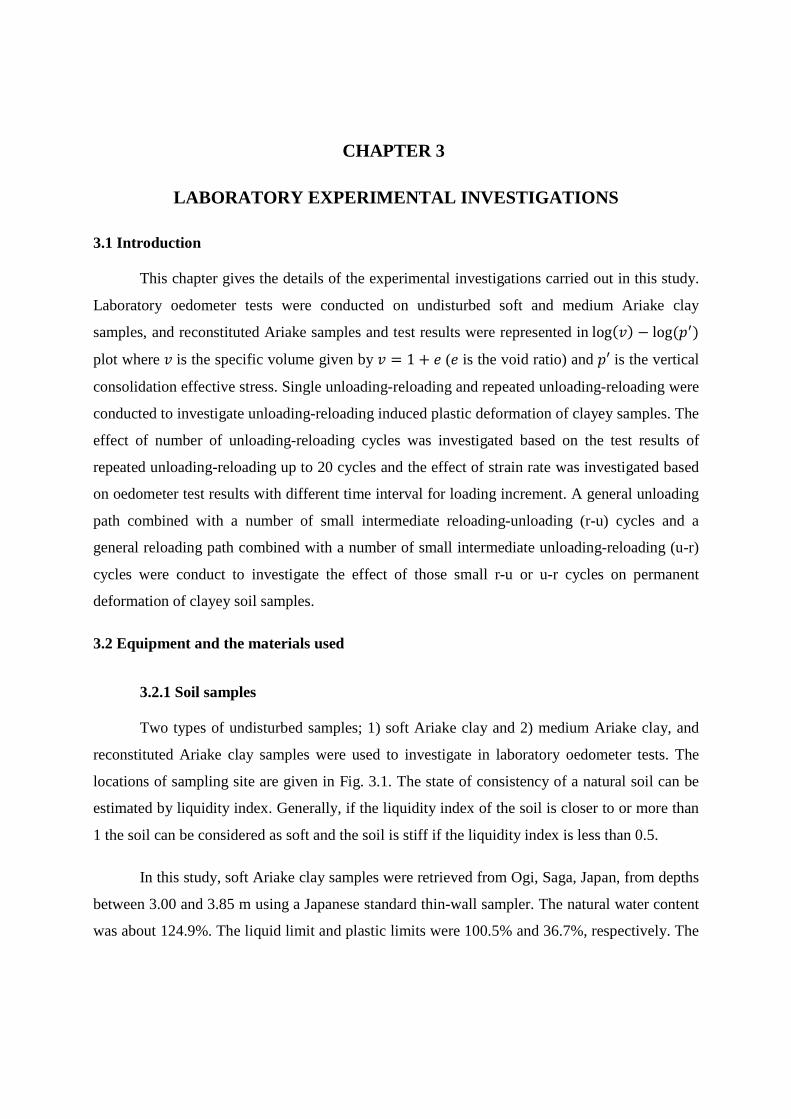
Leroueil (2006) summarized ranges of strain rates encountered in laboratory tests and in

situ as shown in Fig. 2.20. Obviously, the field strain rates are smaller than the strain rate in

laboratory tests. The strain rates in laboratory tests are generally larger than104w�64 ) and for a

standard laboratory oedometer test, the strain late is in the order of 1045�64 ). As for the field

strain rates, it is lower than104w�64 ).

29

Fig. 2.19 Relationship between normalized yield stress, ′� ′��⁄ and strain rate (��) (modified

from Watabe et al. 2012)

Fig. 2.20 Ranges of strain rates encountered in laboratory tests and in situ (Leroueil 2006)

10-10 10-9 10-8 10-7 10-6 10-5 10-40.7

0.8

0.9

1

Osaka Bay Ma13 Ma12 Ma11 Ma10 Ma9 Ma8 Ma7a Ma7b Ma4 Ma3 Ma13Re

p'p/

p'p

0

εv (s-1)

AmagasakiRakusaiAriakeUpper HanedaLower Haneda

LouisevilleOnsoyPisaMexico City

30

2.5 Summary and remarks

Due to excessive pumping of groundwater, many cities around the world have suffered

on-going land-subsidence problem. After strictly regulated or controlled pumping of

groundwater, there has been no further excessive groundwater drawdown. However, there is still

monitored land-subsidence in many areas. The reason considered is due to daily fluctuations of

groundwater as a result of natural phenomena. Various methods for predicting or simulating

land-subsidence due to groundwater level variation have been proposed by many researchers.

One-dimensional (1D) analysis is often used to simulate fluctuations of groundwater level

induced land-subsidence. Butterfield (2011) proposed a sophisticate model that can simulate

unloading-reloading cycle induced plastic deformation of clayey soil sample. However, since the

model assumes that when unloading-reloading in the overconsolidated range, the deformation of

the soil is purely elastic. The model cannot predict plastic deformation under repeated unloading-

reloading in the overconsolidated range. Thus, to predict land-subsidence due to daily fluctuation

of groundwater level, a suitable prediction model must be developed.

CHAPTER 3

LABORATORY EXPERIMENTAL INVESTIGATIONS

3.1 Introduction

This chapter gives the details of the experimental investigations carried out in this study.

Laboratory oedometer tests were conducted on undisturbed soft and medium Ariake clay

samples, and reconstituted Ariake samples and test results were represented inlog�� − log�� plot where � is the specific volume given by � = 1 + � (� is the void ratio) and ′ is the vertical

consolidation effective stress. Single unloading-reloading and repeated unloading-reloading were

conducted to investigate unloading-reloading induced plastic deformation of clayey samples. The

effect of number of unloading-reloading cycles was investigated based on the test results of

repeated unloading-reloading up to 20 cycles and the effect of strain rate was investigated based

on oedometer test results with different time interval for loading increment. A general unloading

path combined with a number of small intermediate reloading-unloading (r-u) cycles and a

general reloading path combined with a number of small intermediate unloading-reloading (u-r)

cycles were conduct to investigate the effect of those small r-u or u-r cycles on permanent

deformation of clayey soil samples.

3.2 Equipment and the materials used

3.2.1 Soil samples

Two types of undisturbed samples; 1) soft Ariake clay and 2) medium Ariake clay, and

reconstituted Ariake clay samples were used to investigate in laboratory oedometer tests. The

locations of sampling site are given in Fig. 3.1. The state of consistency of a natural soil can be

estimated by liquidity index. Generally, if the liquidity index of the soil is closer to or more than

1 the soil can be considered as soft and the soil is stiff if the liquidity index is less than 0.5.

In this study, soft Ariake clay samples were retrieved from Ogi, Saga, Japan, from depths

between 3.00 and 3.85 m using a Japanese standard thin-wall sampler. The natural water content

was about 124.9%. The liquid limit and plastic limits were 100.5% and 36.7%, respectively. The

32

liquidity index was 1.38. Base on the Unified Soil classification System (USCS; ASTM 2006),

the soil is classified as an inorganic clay of high plasticity (CH).

Medium Ariake clay samples were retrieved from Kawasoemachi, Saga, Japan, from

depths between 25.00 and 25.85 m. The natural water content of the soil was about 50%. The

liquid limit and plastic limits were 62.2% and 37.7%, respectively. The liquidity index was 0.5.

Base on the Unified Soil Classification System (USCS; ASTM 2006), the soil is classified as an

inorganic clay of high plasticity (CH).

For the undisturbed samples, after the tubes had been transported into the laboratory, soil

samples were extruded from the thin-wall tubes, sealed with wax, and stored under water for

consolidation tests.

Reconstituted samples were prepared using remoulded Ariake clay obtained from about

2.0 m depth at Ogi, Saga, Japan. The liquid limit and plastic limits were 120.3% and 56.8%,

respectively. The soil was thoroughly mixed with water at a water content of about 1.5 times the

liquid limit, and then consolidated under a pressure of 10 kPa to form reconstituted samples.

3.2.2 Oedometer tests

Most of tests were conducted following JIS A1217 (JSA 2009). The soil sample was 60

mm in diameter and typically 20 mm in height. The vertical consolidation stress was doubled

during each loading increment and reduced half of its previous value during each unloading

increment every 24 hours. Some of the tests were conducted with a 7 day time interval between

two loading increments to investigate the effect of strain rate.

3.3 Test procedures

Two types of test were conducted on the undisturbed and reconstituted samples. One

involved a single unloading-reloading cycle and other involved repeated intermediate unloading-

reloading cycles.

33

Fig. 3.1 Locations of sampling site

3.3.1 Single unloading-reloading

1) A single unloading-reloading cycle was conducted on the undisturbed soft and medium

Ariake clay samples and reconstituted Ariake clay samples, as listed in Table 3.1

2) Oedometer tests with time interval between successive loading increments of 1 day

and 7 days were conducted using the medium Ariake clay samples to investigate the effect of

strain rate. The tested cases are also listed in Table 3.1.

3.3.2 Repeated intermediate unloading-reloading

1) Four cycles of repeated unloading-reloading were conducted on the undisturbed soft

and medium Ariake clay samples and reconstituted Ariake clay samples as listed in Table 3.2.

The results were used to investigate whether such loading cycles would induce plastic

deformation.

34

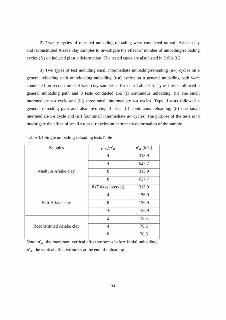
2) Twenty cycles of repeated unloading-reloading were conducted on soft Ariake clay

and reconstituted Ariake clay samples to investigate the effect of number of unloading-reloading

cycles (�) on induced plastic deformation. The tested cases are also listed in Table 3.2.

3) Two types of test including small intermediate unloading-reloading (u-r) cycles on a

general reloading path or reloading-unloading (r-u) cycles on a general unloading path were

conducted on reconstituted Ariake clay sample as listed in Table 3.3. Type I tests followed a

general unloading path and 3 tests conducted are: (i) continuous unloading, (ii) one small

intermediate r-u cycle and (iii) three small intermediate r-u cycles. Type II tests followed a

general reloading path and also involving 3 tests: (i) continuous reloading, (ii) one small

intermediate u-r cycle and (iii) four small intermediate u-r cycles. The purpose of the tests is to

investigate the effect of small r-u or u-r cycles on permanent deformation of the sample.

Table 3.1 Single unloading-reloading testsTable

Samples ′� ′�⁄ ′� (kPa)

Medium Ariake clay

4 313.9

4 627.7

8 313.9

8 627.7

8 (7 days interval) 313.9

Soft Ariake clay

4 156.9

8 156.9

16 156.9

Reconstituted Ariake clay

2 78.5

4 78.5

8 78.5

Note: ′�, the maximum vertical effective stress before initial unloading;

′�, the vertical effective stress at the end of unloading.

35

Table 3.2 Repeated unloading-reloading tests

Type of tests Samples ′� ′�⁄ ′� (kPa) ′� ′�⁄ ′� (kPa)

Repeated unloading-

reloading 4 cycles

Medium Ariake clay

4 313.9 4 313.9

4 627.7 4 627.7

4 313.9 2 156.9

4 627.7 2 313.9

8 313.9 8 313.9

8 627.7 8 627.7

8 313.9 4 156.9

8 627.7 4 156.9

16 313.9 2 39.2

Soft Ariake clay

4 156.9 4 156.9

4 156.9 2 78.5

8 156.9 8 156.9

8 156.9 4 78.5

Reconstituted Ariake

clay

2 78.5 2 78.5

2 78.5 1.5 58.9

4 78.5 4 78.5

4 78.5 2 39.2

8 78.5 8 78.5

8 78.5 4 39.2

16 78.5 2 9.8

Repeated unloading-

reloading 20 cycles

Reconstituted Ariake

clay

2 78.5 2 78.5

4 78.5 2 39.2

Soft Ariake clay 2 78.5 2 78.5

4 78.5 2 39.2

Note: ′�, the intermediate unloading pressure.

36

Table 3.3 Small intermediate unloading-reloading test

Type of

tests

Samples Loading types ′�

(kPa)

′�

(kPa)

′�

(kPa)

Type I Reconstituted

Ariake clay

Continuous

unloading

78.8 9.8 -

Small r-u 1

cycle

78.8 39.2, 9.8 58.9

Small r-u 3

cycles

78.8 39.2, 29.4, 19.6,

9.8

58.9, 39.2, 29.4

Type II Reconstituted

Ariake clay

Continuous

reloading

156.9 19.6 -

Small u-r 1

cycle

156.9 19.6, 39.2 78.5

Small u-r 4

cycles

156.9 19.6, 29.4, 39.2,

58.9, 78.5

39.2, 58.5, 78.5,

117.7

37

3.4 Results and discussions

3.4.1 Single unloading-reloading cycle

Figures 3.2 and 3.3 show the unloading-reloading curves of the undisturbed soft and

medium Ariake clay samples in log�� − log�� diagram, respectively. It can be observed that

the unloading curve is close to linear, and reloading curve is non-linear, which supports the

assumption made by Butterfield (2011). Fig. 3.4 shows unloading-reloading curves of the

reconstituted Ariake clay samples. It can be also seen that the unloading curve is close to linear,

and reloading curve is non-linear. However, for reconstituted Ariake clay that does not have a

microstructure, the test results show that the virgin compression line is not exactly linear in a

log�� − log��relationship. Three single unloading-reloading curves with different ′� ′�⁄

values (′� ′�⁄ = 2, 4, 8) of reconstituted Ariake clay samples are compared in Fig. 3.5. It can

be seen from the figure that the plastic deformation induced by cycle of unloading-reloading is a

function of′� ′�⁄ . Increasing the value of′� ′�⁄ will increase amount of plastic deformation

at the end of reloading.

3.4.2 Repeated intermediate unloading- reloading cycles

Figures 3.6 to 3.10 show the test results of repeated intermediate unloading-reloading

(four cycles) using undisturbed and reconstituted Ariake clay samples in log�� − log�� plot.

These figures clearly show that intermediate unloading-reloading process is not purely elastic.

There is continuous increase of plastic deformation with the increase of the number of loading

cycles. Obviously, it is different from the assumption made by Butterfield (2011) that unloading-

reloading in an overconsolidated range will not cause plastic deformation. For undisturbed

sample which is microstructured and virgin compression is usually associated with some kind of

destructuring effect. It is considered that the repeated unloading-reloading cycles caused

permanent deformation perhaps due partially to the destructuring effect. Comparing figure (a)

and (b) in Figs. 3.6 to 3.10 show that for a given value of′� ′�⁄ , the plastic strain increment is

a function of′� ′�⁄ . The larger the value of′� ′�⁄ , the larger is the plastic strain increment.

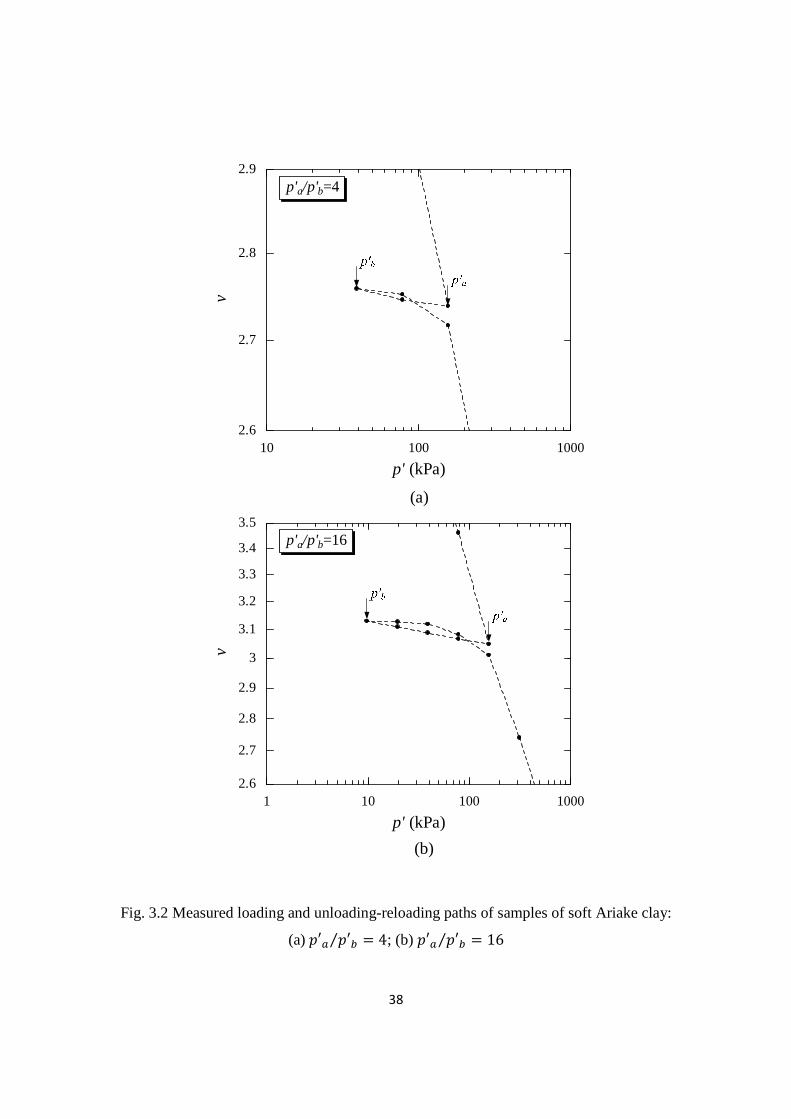
38

10 100 10002.6

2.7

2.8

2.9

v

p' (kPa)

p'a/p'b=4

(a)

1 10 100 10002.6

2.7

2.8

2.9

3

3.1

3.2

3.3

3.4

3.5

v

p' (kPa)

p'a/p'b=16

(b)

Fig. 3.2 Measured loading and unloading-reloading paths of samples of soft Ariake clay:

(a)′� ′�⁄ = 4; (b) ′� ′�⁄ = 16

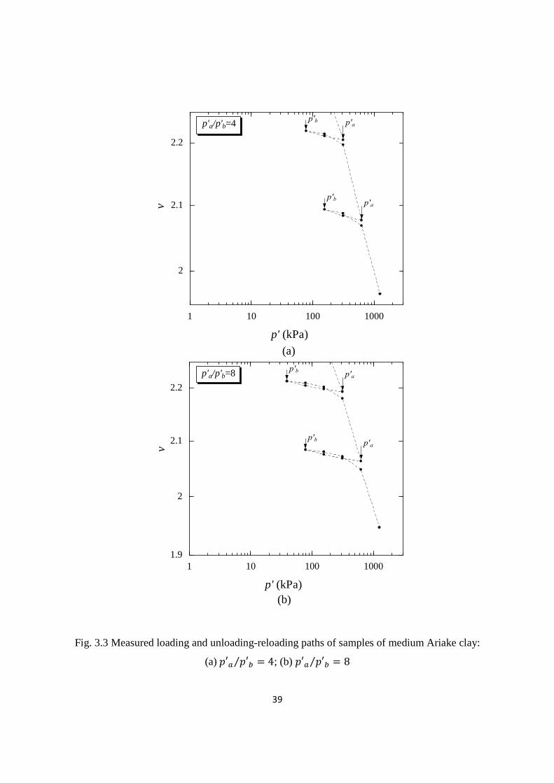
39

1 10 100 10001.9

2

2.1

2.2

v

p' (kPa)

p'a/p'b=8

(b)

1 10 100 1000

2

2.1

2.2

v

p' (kPa)

p'a/p'b=4

(a)

p′ap′b

p′ap′b

p′ap′b

p′ap′b

Fig. 3.3 Measured loading and unloading-reloading paths of samples of medium Ariake clay:

(a)′� ′�⁄ = 4; (b) ′� ′�⁄ = 8

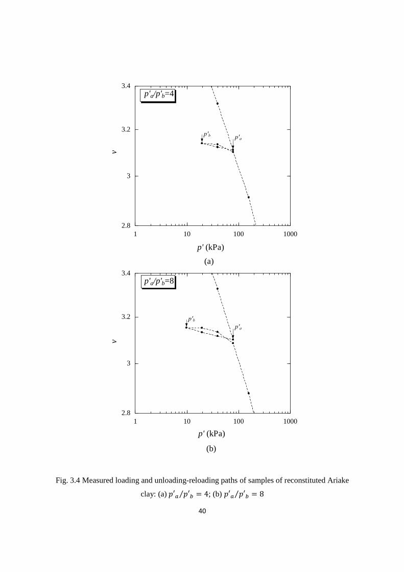
40

1 10 100 10002.8

3

3.2

3.4

v

p' (kPa)

p'a/p'b=4

(a)

1 10 100 10002.8

3

3.2

3.4

v

p' (kPa)

p'a/p'b=8

(b)

p′a

p′b

p′ap′b

Fig. 3.4 Measured loading and unloading-reloading paths of samples of reconstituted Ariake

clay: (a)′� ′�⁄ = 4; (b) ′� ′�⁄ = 8

41

Fig. 3.5 Effect of the value of ′� ′�⁄ on induced plastic deformation of reconstituted Ariake

samples

1 10 100

3.1

3.2v

p' (kPa)

p'a/p'b=2 p'a/p'b=4 p'a/p'b=8

3.05

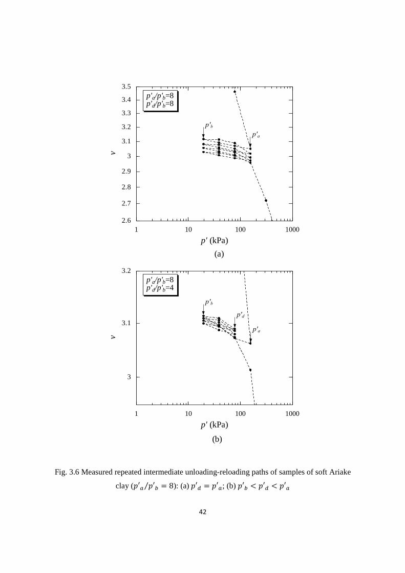
42

1 10 100 10002.6

2.7

2.8

2.9

3

3.1

3.2

3.3

3.4

3.5

v

p' (kPa)

p'a/p'b=8p'd/p'b=8

(a)

1 10 100 1000

3

3.1

3.2

v

p' (kPa)

p'a/p'b=8p'd/p'b=4

(b)

p′a

p′b

p′a

p′b

p′d


clay (′� ′�⁄ = 8): (a)′� = ′�; (b) ′� < ′� < ′�

43

10 100 10002.5

2.6

2.7

2.8

2.9

v

p' (kPa)

p'a/p'b=4p'd/p'b=4

(a)

10 100 10002.6

2.7

2.8

v

p' (kPa)

p'a/p'b=4p'd/p'b=2

(b)


clay (′� ′�⁄ = 4): (a)′� = ′�; (b) ′� < ′� < ′�

44

10 100 10002.1

2.2

v

p' (kPa)

p'a/p'b=8p'd/p'b=4

(b) p'b<p'd<p'a

10 100 1000

2.1

2.2

v

p' (kPa)

p'a/p'b=8p'd/p'b=8

(a) p'd=p'a


Ariake clay (′� ′�⁄ = 8): (a)′� = ′�; (b) ′� < ′� < ′�

45

10 100 10002

2.1

v

p' (kPa)

p'a/p'b=4p'd/p'b=4

(a)

10 100 1000

2

2.1

v

p' (kPa)

p'a/p'b=4p'd/p'b=2

(b)


Ariake clay (′� ′�⁄ = 4): (a)′� = ′�; (b) ′� < ′� < ′�

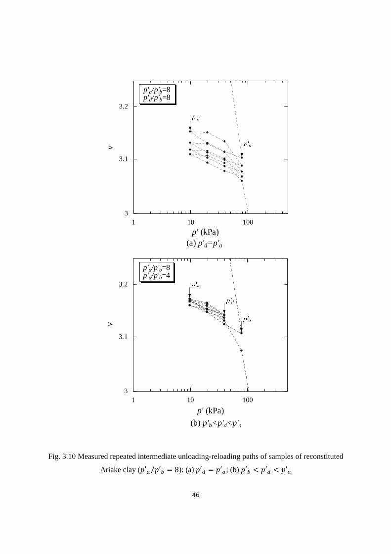
46

1 10 1003

3.1

3.2v

p' (kPa)

p'a/p'b=8p'd/p'b=8

(a) p'd=p'a

1 10 1003

3.1

3.2

v

p' (kPa)

p'a/p'b=8p'd/p'b=4

(b) p'b<p'd<p'a

Fig. 3.10 Measured repeated intermediate unloading-reloading paths of samples of reconstituted

Ariake clay (′� ′�⁄ = 8): (a)′� = ′�; (b) ′� < ′� < ′�

47

3.4.3 Effect of small intermediate unloading-reloading (r-u) and reloading-unloading

(u-r) cycle

Based on the data reported by Sakai (2001), it can be seen that small fluctuations on a

general trend of reduction or recovery of groundwater level can induce compression of clayey

soil deposit (see Fig. 2.6). To investigate the effect of small reloading-unloading (or unloading-

reloading) process on permanent deformation of clayey soil, oedometer tests of general

unloading combined with different number of small cycles of reloading-unloading (r-u) (Type I

tests); and general reloading combined with different number of small cycles of unloading-

reloading (u-r) (Type II tests), were conducted using reconstituted Ariake clay samples. Fig. 3.11

shows the results of Type I tests. The results clearly show that the sample subjected to the small

intermediate r-u cycle(s) had smaller rebound, i.e., the small intermediate r-u cycles on a general

unloading path induced plastic strain increment. It is also seen that the amount of plastic

deformation increased by increase of number of small intermediate r-u cycles.

Fig. 3.12 shows the results of Type II tests. It can be seen that the small intermediate u-r

cycles caused smaller plastic deformation and the amount of plastic deformation decreased with

the number of the small intermediate u-r cycles.

The fundamental physical reason for this kind of phenomenon is that the deformation of

soil is stress history dependent and generally an unloading-reloading cycle will cause a hysteresis

loop. The results presented in Figs 3.11 and 3.12 have an important application for predicting

daily groundwater fluctuation induced land-subsidence.

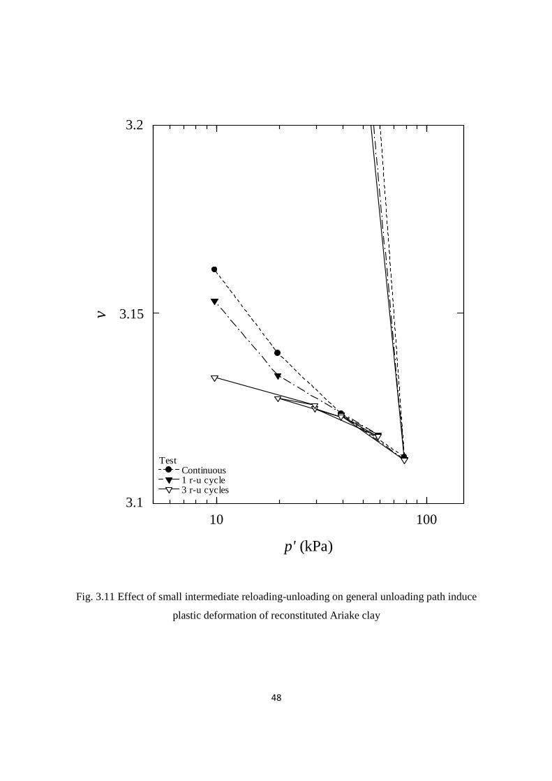
48

Fig. 3.11 Effect of small intermediate reloading-unloading on general unloading path induce

plastic deformation of reconstituted Ariake clay

10 1003.1

3.2

Test Continuous 1 r-u cycle 3 r-u cycles

p' (kPa)

3.15v

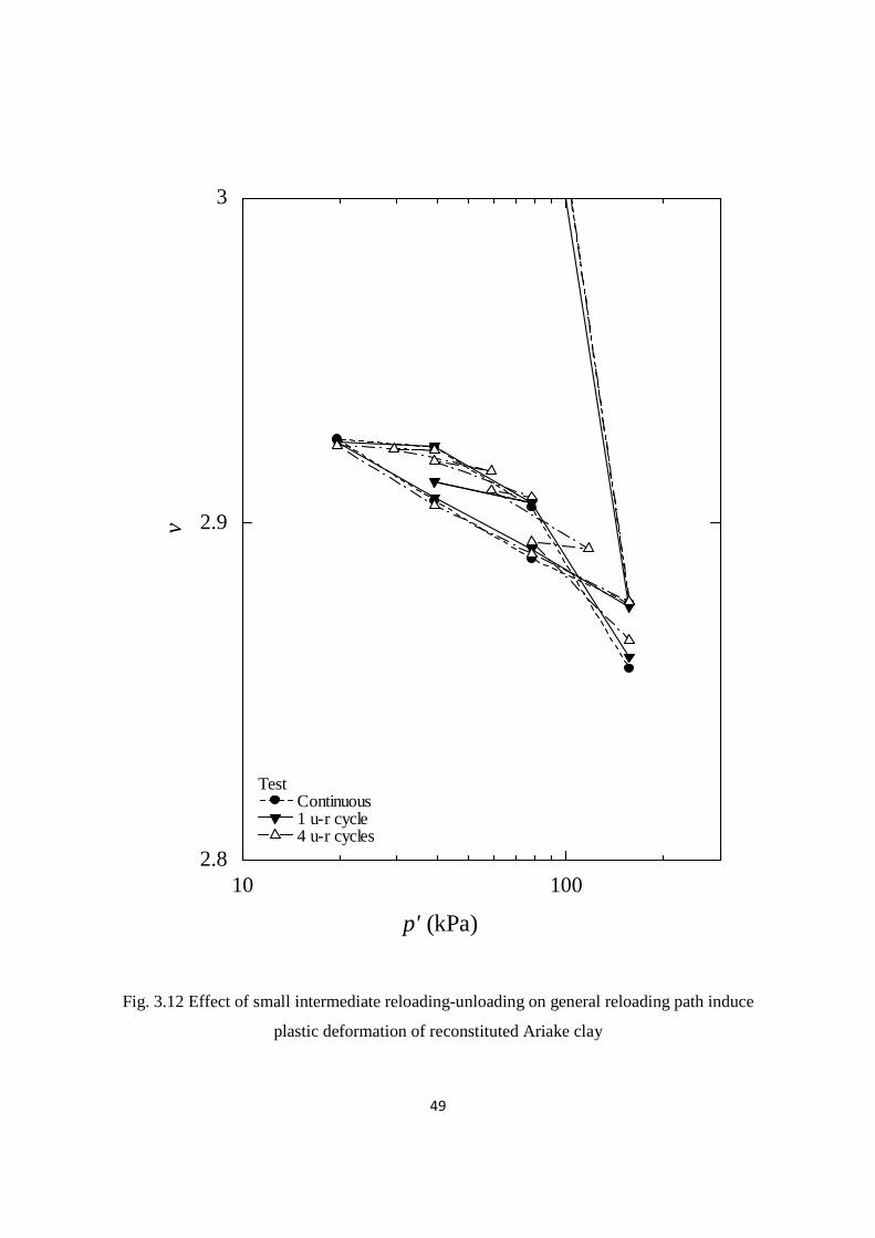
49

Fig. 3.12 Effect of small intermediate reloading-unloading on general reloading path induce

plastic deformation of reconstituted Ariake clay

10 1002.8

2.9

3v

p' (kPa)

Test Continuous 1 u-r cycle 4 u-r cycles

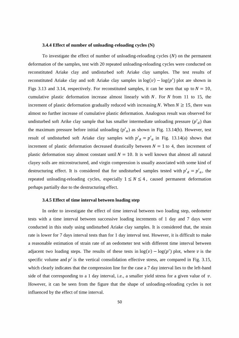
50

3.4.4 Effect of number of unloading-reloading cycles (N)

To investigate the effect of number of unloading-reloading cycles (�) on the permanent

deformation of the samples, test with 20 repeated unloading-reloading cycles were conducted on

reconstituted Ariake clay and undisturbed soft Ariake clay samples. The test results of

reconstituted Ariake clay and soft Ariake clay samples in log�� − log��plot are shown in

Figs 3.13 and 3.14, respectively. For reconstituted samples, it can be seen that up to� = 10,

cumulative plastic deformation increase almost linearly with� . For � from 11 to 15, the

increment of plastic deformation gradually reduced with increasing�. When� ≥ 15, there was

almost no further increase of cumulative plastic deformation. Analogous result was observed for

undisturbed soft Arike clay sample that has smaller intermediate unloading pressure (′�) than

the maximum pressure before initial unloading (′�) as shown in Fig. 13.14(b). However, test

result of undisturbed soft Ariake clay samples with ′� = ′� in Fig. 13.14(a) shows that

increment of plastic deformation decreased drastically between � = 1 to 4, then increment of

plastic deformation stay almost constant until� = 10. It is well known that almost all natural

clayey soils are microstructured, and virgin compression is usually associated with some kind of

destructuring effect. It is considered that for undisturbed samples tested with′� = ′� , the

repeated unloading-reloading cycles, especially1 ≤ � ≤ 4 , caused permanent deformation

perhaps partially due to the destructuring effect.

3.4.5 Effect of time interval between loading step

In order to investigate the effect of time interval between two loading step, oedometer

tests with a time interval between successive loading increments of 1 day and 7 days were

conducted in this study using undisturbed Ariake clay samples. It is considered that, the strain

rate is lower for 7 days interval tests than for 1 day interval test. However, it is difficult to make

a reasonable estimation of strain rate of an oedometer test with different time interval between

adjacent two loading steps. The results of these tests in log�� − log�� plot, where � is the

specific volume and is the vertical consolidation effective stress, are compared in Fig. 3.15,

which clearly indicates that the compression line for the case a 7 day interval lies to the left-hand

side of that corresponding to a 1 day interval, i.e., a smaller yield stress for a given value of�.

However, it can be seen from the figure that the shape of unloading-reloading cycles is not

influenced by the effect of time interval.

51

3.5 Summary

Base on the test results presented in this chapter, the following summary can be made.

(1) For undisturbed soft and medium Ariake clay samples and reconstituted Ariake clay

samples, the test results of single unloading-reloading indicate that in log�� − log�� plot,

unloading path is close to linear. However, the reloading path is non-linear. Here � is the specific

volume given by � = 1 + � (where � is the void ratio) and ’ is the vertical consolidation

pressure.

(2) The test results indicate that repeated unloading-reloading cycles even in

overconsolidation region can induce plastic deformation.

(3) For reconstituted Ariake samples, for a general unloading path, small intermediate

reloading-unloading (r-u) cycles caused increase of permanent deformation. And for a general

unloading path, small intermediate unloading-reloading (u-r) cycles caused reduction of

permanent deformation.

52

20 30 40 50 60 70 80 901003

3.1

3.2

v

p' (kPa)

p'a/p'b=2p'd/p'b=2

(a) p'b<p'd=p'a

10 20 30 40 50 60 70 8090

3.1v

p' (kPa)

p'a/p'b=4p'd/p'b=2

3.08

3.12

(b) p'b<p'd<p'a

Fig. 3.13 Effect of number of unloading-reloading cycles (reconstituted Ariake clay samples)

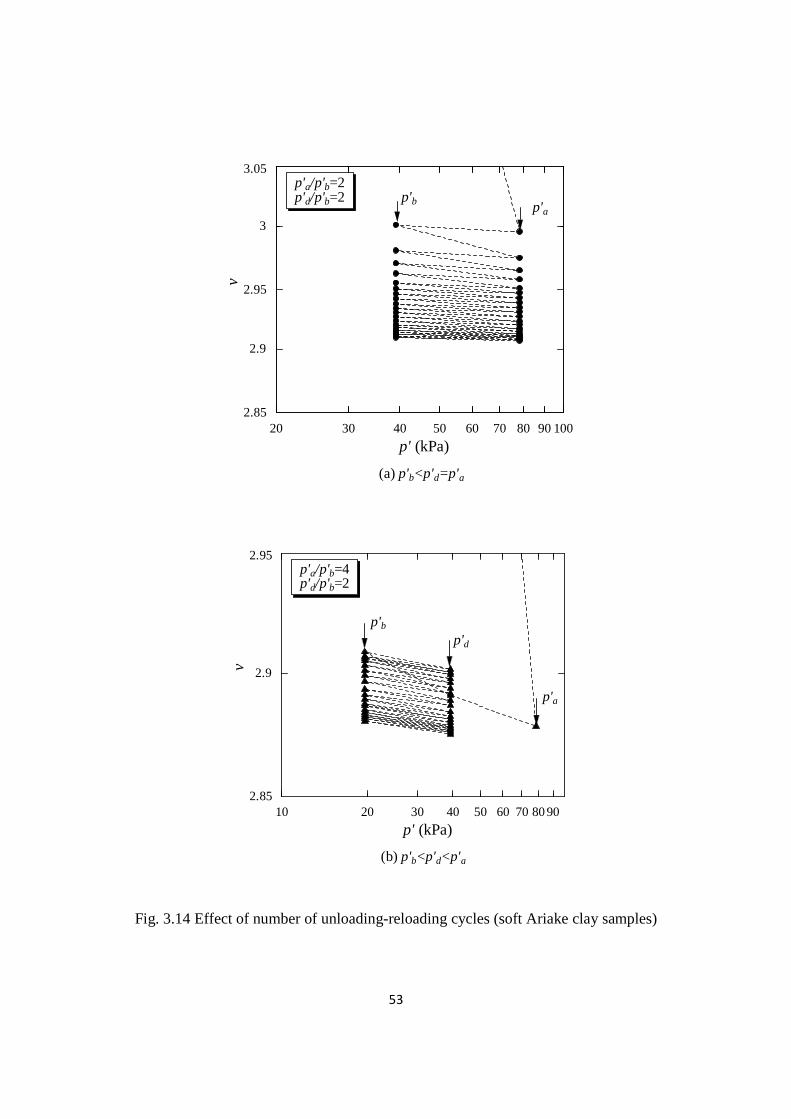
53

Fig. 3.14 Effect of number of unloading-reloading cycles (soft Ariake clay samples)

20 30 40 50 60 70 80 90100

2.9

3v

p' (kPa)

p'a/p'b=2p'd/p'b=2

(a) p'b<p'd=p'a

p'ap'b

2.85

3.05

2.95

10 20 30 40 50 60 70 8090

2.9v

p' (kPa)

p'a/p'b=4p'd/p'b=2

2.95

2.85

(b) p'b<p'd<p'a

p'a

p'd

p'b

54

1 10 100 1000

2

2.2

2.4

2.6

2.8

3

3.2

v

p' (kPa)

p'a/p'b=8

1 day interval7 days interval

Fig. 3.15 Effect of time interval between two loading steps on yield stress of undisturbed Ariake

clay

CHAPTER 4

THEORETICAL MODELLING

4.1 Introduction

Butterfield (2011) proposed a model for unloading-reloading induced plastic deformation

of a clayey soil. The model can predict deformation behaviour of single unloading-reloading of

many natural clayey soils well. In this study, the model was used to predict deformation

behaviour of undisturbed and reconstituted Ariake clay samples under single unloading-

reloading cycles also. However, since the model assume that when unloading-reloading in an

overconsolidated range, i.e., so-called “intermediate” unloading-reloading, the deformation is

purely elastic and the model cannot predict plastic deformation induced by repeated unloading-

reloading cycles. A modified unloading-reloading model was proposed based on the Butterfield

model. The usefulness of the modified model is discussed based on a comparison of the

simulated and measured results of the undisturbed soft and medium Ariake clay samples and

reconstituted Ariake clay samples.

4.2 Predicting unloading-reloading cycle by Butterfield’s unloading-reloading model

4.2.1 Butterfield’s unloading-reloading model

Butterfield (2011) proposed a model for unloading-reloading induced one-dimensional

deformation of clayey soils. The basic assumptions adopted are as follows.

(1) The virgin compression and the unloading lines are linear in a log�� − log�� plot, where

′ is the consolidation pressure (vertical effective stress), and � is the specific volume given by

� = 1 + � (where � is the void ratio). In this plot the slope of the virgin loading line is denoted

as #′� and that of the unloading line is #′$. (2) For reloading, the log�� − log�� relationship is non-linear and can be expressed by the

following exponential function:

�/�� = bc dR efg[` W h1 − i �f�fjk

[` lm (2.10bis)

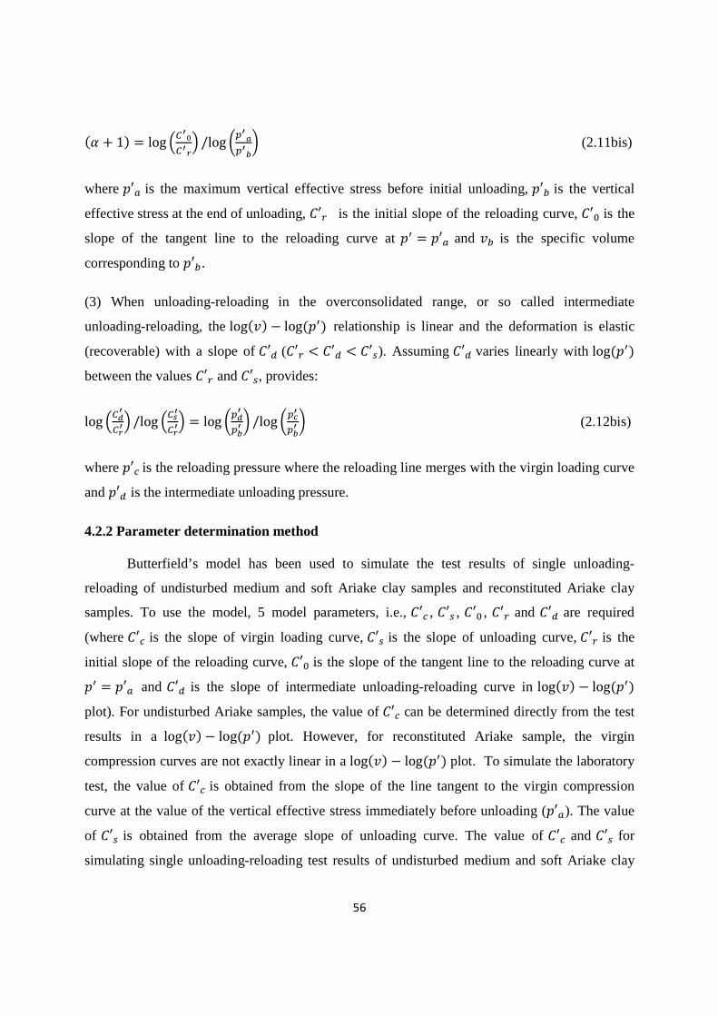
56

�@ + 1� = log RefnefgW /logi�fV�fjk (2.11bis)

where ′�is the maximum vertical effective stress before initial unloading, ′� is the vertical

effective stress at the end of unloading, #′) is the initial slope of the reloading curve, #′� is the

slope of the tangent line to the reloading curve at = ′� and �� is the specific volume

corresponding to ′�.

(3) When unloading-reloading in the overconsolidated range, or so called intermediate

unloading-reloading, the log�� − log�� relationship is linear and the deformation is elastic

(recoverable) with a slope of #′� (#′) < #′� < #′$). Assuming #′� varies linearly with log�� between the values #′) and #′$, provides:

logReofegfW /logRepf

egfW = log i�of�jfk /log i�qf�jfk (2.12bis)

where ′� is the reloading pressure where the reloading line merges with the virgin loading curve

and ′� is the intermediate unloading pressure.

4.2.2 Parameter determination method

Butterfield’s model has been used to simulate the test results of single unloading-

reloading of undisturbed medium and soft Ariake clay samples and reconstituted Ariake clay

samples. To use the model, 5 model parameters, i.e.,#′� ,#′$ ,#′� , #′) and #′� are required

(where #′� is the slope of virgin loading curve,#′$ is the slope of unloading curve,#′) is the

initial slope of the reloading curve, #′� is the slope of the tangent line to the reloading curve at

= ′� and #′� is the slope of intermediate unloading-reloading curve in log�� − log�� plot). For undisturbed Ariake samples, the value of #′� can be determined directly from the test

results in a log�� − log�� plot. However, for reconstituted Ariake sample, the virgin

compression curves are not exactly linear in a log�� − log�� plot. To simulate the laboratory

test, the value of #′� is obtained from the slope of the line tangent to the virgin compression

curve at the value of the vertical effective stress immediately before unloading (′�). The value

of #′$ is obtained from the average slope of unloading curve. The value of#′� and#′$ for

simulating single unloading-reloading test results of undisturbed medium and soft Ariake clay

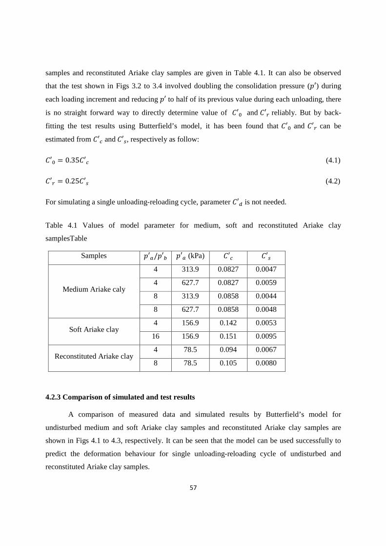
57

samples and reconstituted Ariake clay samples are given in Table 4.1. It can also be observed

that the test shown in Figs 3.2 to 3.4 involved doubling the consolidation pressure (′) during

each loading increment and reducing ′ to half of its previous value during each unloading, there

is no straight forward way to directly determine value of #′� and #′) reliably. But by back-

fitting the test results using Butterfield’s model, it has been found that #′� and #′) can be

estimated from #′� and#′$, respectively as follow:

#′� = 0.35#′� (4.1)

#′) = 0.25#′$ (4.2)

For simulating a single unloading-reloading cycle, parameter #′� is not needed.

Table 4.1 Values of model parameter for medium, soft and reconstituted Ariake clay

samplesTable

Samples ′�/′� ′� (kPa) #′� #′$

Medium Ariake caly

4 313.9 0.0827 0.0047

4 627.7 0.0827 0.0059

8 313.9 0.0858 0.0044

8 627.7 0.0858 0.0048

Soft Ariake clay 4 156.9 0.142 0.0053

16 156.9 0.151 0.0095

Reconstituted Ariake clay 4 78.5 0.094 0.0067

8 78.5 0.105 0.0080

4.2.3 Comparison of simulated and test results

A comparison of measured data and simulated results by Butterfield’s model for

undisturbed medium and soft Ariake clay samples and reconstituted Ariake clay samples are

shown in Figs 4.1 to 4.3, respectively. It can be seen that the model can be used successfully to

predict the deformation behaviour for single unloading-reloading cycle of undisturbed and

reconstituted Ariake clay samples.

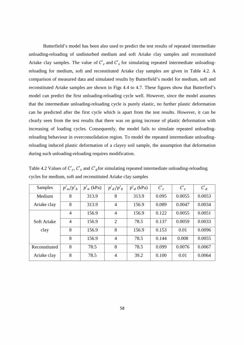
58

Butterfield’s model has been also used to predict the test results of repeated intermediate

unloading-reloading of undisturbed medium and soft Ariake clay samples and reconstituted

Ariake clay samples. The value of#′�and #′$ for simulating repeated intermediate unloading-

reloading for medium, soft and reconstituted Ariake clay samples are given in Table 4.2. A

comparison of measured data and simulated results by Butterfield’s model for medium, soft and

reconstituted Ariake samples are shown in Figs 4.4 to 4.7. These figures show that Butterfied’s

model can predict the first unloading-reloading cycle well. However, since the model assumes

that the intermediate unloading-reloading cycle is purely elastic, no further plastic deformation

can be predicted after the first cycle which is apart from the test results. However, it can be

clearly seen from the test results that there was on going increase of plastic deformation with

increasing of loading cycles. Consequently, the model fails to simulate repeated unloading-

reloading behaviour in overconsolidation region. To model the repeated intermediate unloading-

reloading induced plastic deformation of a clayey soil sample, the assumption that deformation

during such unloading-reloading requires modification.

Table 4.2 Values of#′�,#′$ and #′�for simulating repeated intermediate unloading-reloading

cycles for medium, soft and reconstituted Ariake clay samples

Samples ′�/′� ′� (kPa) ′�/′� ′� (kPa) #′� #′$ #′�

Medium

Ariake clay

8 313.9 8 313.9 0.095 0.0055 0.0053

8 313.9 4 156.9 0.089 0.0047 0.0034

Soft Ariake

clay

4 156.9 4 156.9 0.122 0.0055 0.0051

4 156.9 2 78.5 0.137 0.0059 0.0033

8 156.9 8 156.9 0.153 0.01 0.0096

8 156.9 4 78.5 0.144 0.008 0.0055

Reconstituted

Ariake clay

8 78.5 8 78.5 0.099 0.0076 0.0067

8 78.5 4 39.2 0.100 0.01 0.0064

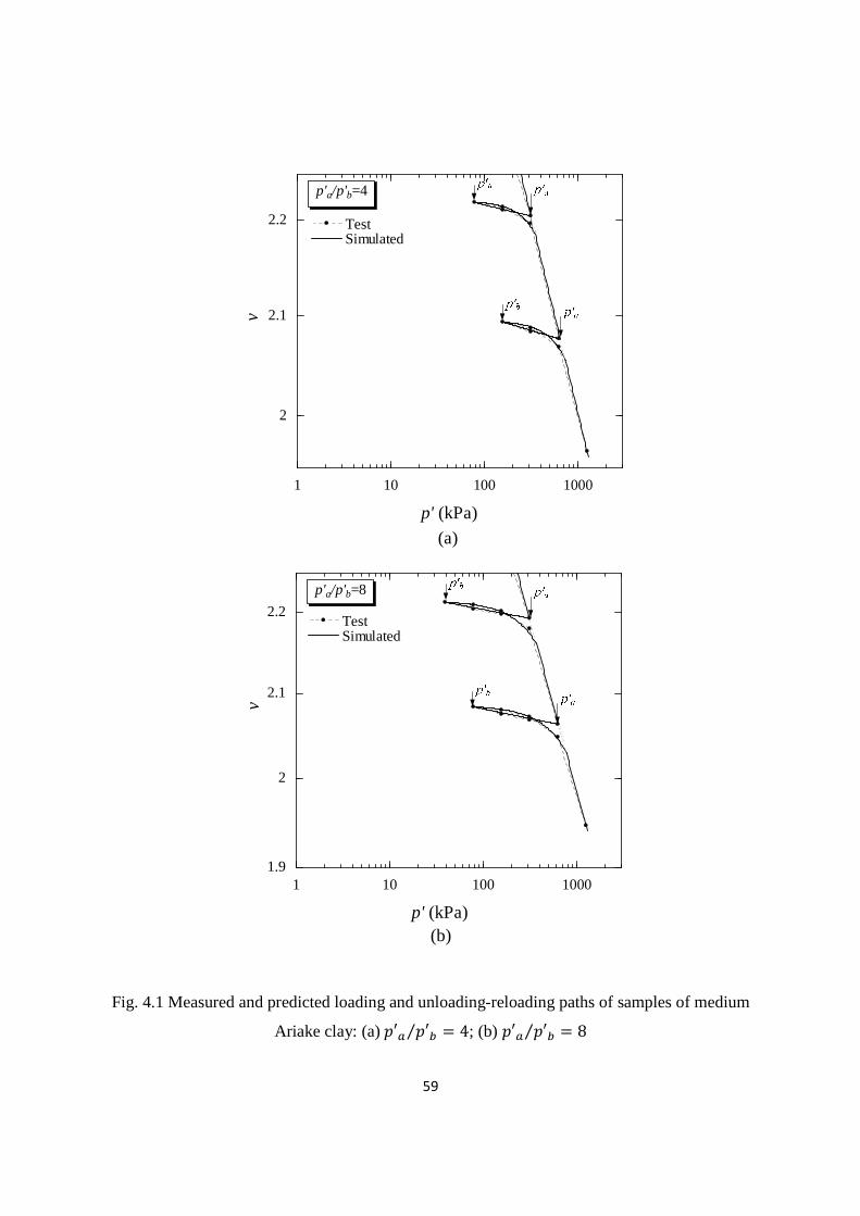
59

1 10 100 1000

2

2.1

2.2

v

p' (kPa)

p'a/p'b=4

Test Simulated

(a)

1 10 100 10001.9

2

2.1

2.2

v

p' (kPa)

p'a/p'b=8

Test Simulated

(b)

Fig. 4.1 Measured and predicted loading and unloading-reloading paths of samples of medium

Ariake clay: (a)′� ′�⁄ = 4; (b) ′� ′�⁄ = 8

60

10 100 10002.6

2.7

2.8

2.9

v

p' (kPa)

p'a/p'b=4

test simulated

(a)

1 10 100 10002.6

2.7

2.8

2.9

3

3.1

3.2

3.3

3.4

3.5

v

p' (kPa)

p'a/p'b=16

Test Simulated

(b)

Fig. 4.2 Measured and predicted loading and unloading-reloading paths of samples of soft Ariake

clay: (a)′� ′�⁄ = 4; (b) ′� ′�⁄ = 16

61

1 10 100 10002.8

3

3.2

3.4

v

p' (kPa)

p'a/p'b=4

test simulated

(a)

1 10 100 10002.8

3

3.2

3.4

v

p' (kPa)

p'a/p'b=8

test simulated

(b)

p′ap′b

p′a

p′b

Fig. 4.3 Measured and predicted loading and unloading-reloading paths of samples of

reconstituted Ariake clay: (a)′� ′�⁄ = 4; (b) ′� ′�⁄ = 8

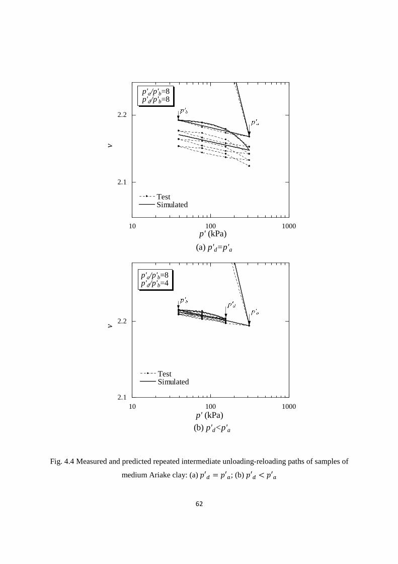
62

10 100 1000

2.1

2.2v

p' (kPa)

p'a/p'b=8p'd/p'b=8

Test Simulated

(a) p'd=p'a

10 100 10002.1

2.2v

p' (kPa)

p'a/p'b=8p'd/p'b=4

Test Simulated

(b) p'd<p'a


medium Ariake clay: (a)′� = ′�; (b) ′� < ′�

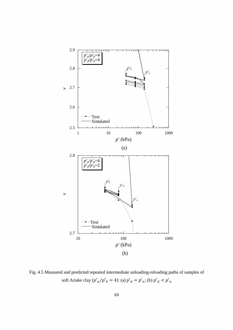
63

1 10 100 10002.5

2.6

2.7

2.8

2.9

v

p' (kPa)

p'a/p'b=4p'd/p'b=4

Test Simulated

(a)

10 100 10002.7

2.8

v

p' (kPa)

p'a/p'b=4p'd/p'b=2

Test Simulated

(b)


soft Ariake clay (′� ′�⁄ = 4): (a)′� = ′�; (b) ′� < ′�

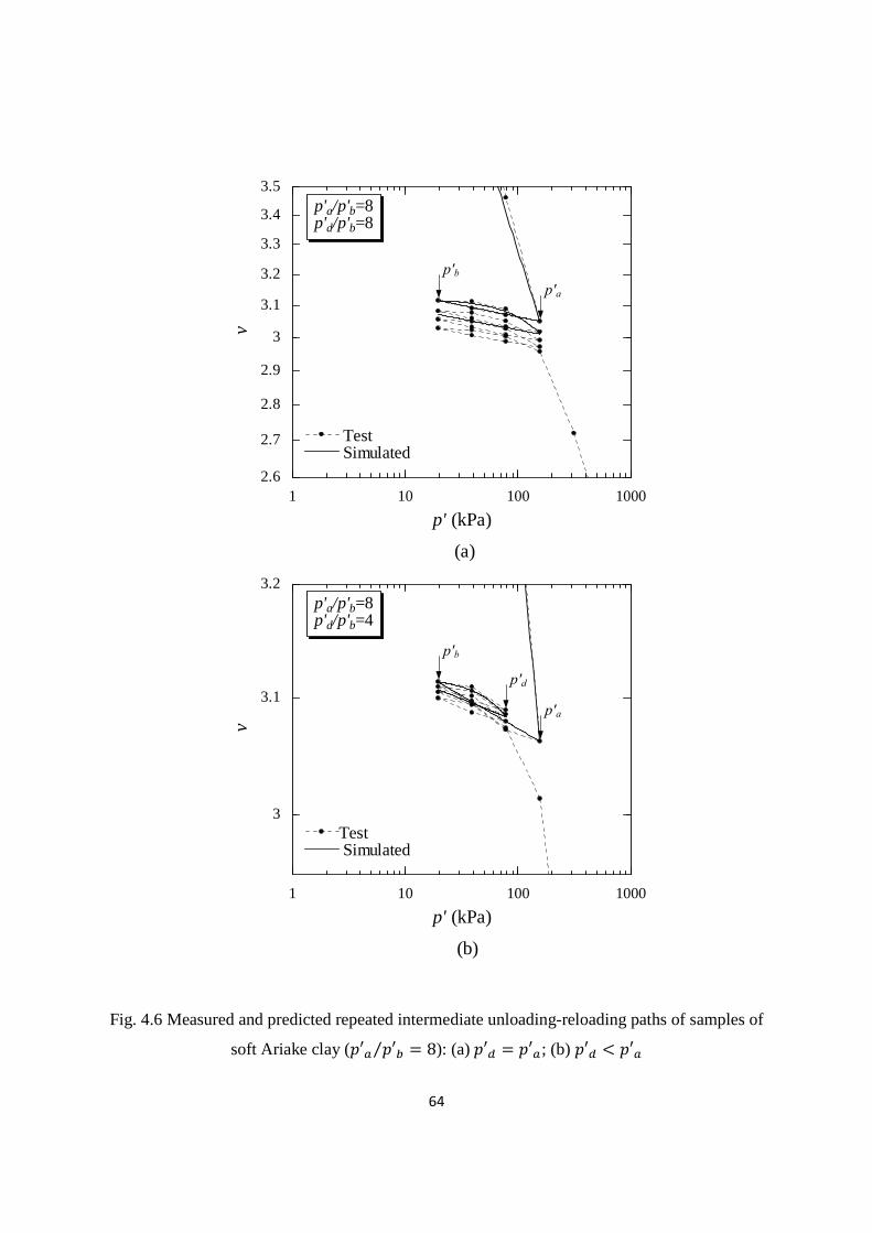
64

1 10 100 10002.6

2.7

2.8

2.9

3

3.1

3.2

3.3

3.4

3.5

v

p' (kPa)

p'a/p'b=8p'd/p'b=8

Test Simulated

(a)

1 10 100 1000

3

3.1

3.2

v

p' (kPa)

p'a/p'b=8p'd/p'b=4

Test Simulated

(b)

p′a

p′b

p′d

p′a

p′b


soft Ariake clay (′� ′�⁄ = 8): (a)′� = ′�; (b) ′� < ′�

65

1 10 1003

3.1

3.2v

p' (kPa)

p'a/p'b=8p'd/p'b=8

test simulated

(a) p'd=p'a

1 10 1003

3.1

3.2

v

p' (kPa)

p'a/p'b=8p'd/p'b=4

test simulated

(b) p'd<p'a


reconstituted Ariake clay: (a)′� = ′�; (b) ′� < ′�

66

4.3 Modified unloading-reloading model

4.3.1 Proposed intermediate unloading-reloading curve

For simulating the deformation induced by repeated intermediate unloading-reloading,

the assumption made by Butterfield (2011) that deformation during unloading-reloading in

overconsolidated region is purely elastic required modification. Based on the results of

laboratory tests on undisturbed soft and medium Ariake clay samples and reconstituted Ariake

clay samples conducted in this study (see in Chapter 3), it was noted that the intermediate

unloading is close to linear in a log�� − log�� plot, and Butterfield’s assumption is acceptable.

However, the intermediate reloading curve is not linear, and repeated intermediate unloading-

reloading will induce plastic deformation. Mathematically, the intermediate reloading curve can

be expressed by Eqs 2.10 and 2.11.

However, the means of determining parameter#′� in Eq. (2.11) and parameter #′� for

simulating intermediate unloading curve in Eq. (2.12) need to be modified. In plasticity theory,

any permanent change on volumetric strain is related to a change of the size of yield locus (strain

hardening). The permanent volumetric strain caused by the repeated intermediate unloading-

reloading cycles, will also influence the “size of yield locus” of the sample. In this study, it is

proposed to use ′� to indicate the “size of yield locus”, and a method has been proposed to

consider the change of ′� during repeated intermediate unloading-reloading.

4.3.2 Parameter determination

(a) Calculating new ′� value

Let’s denote the new ′� value as′�". As illustrated in Fig. 4.8(a), assuming both the

first and second unloading are to the same pressure ′�, and a permanent change on � value of

(�� − ��") is resulted, then the value of ′�" can be calculated as follow:

′�" = �Vf��j} �jO⁄ �~O �qf⁄ � (4.3)

Eq. (4.3) has been derived under the condition that when consolidation pressure increases from

′� to′�", the virgin compression will induce a change of specific volume (�� − ��").

67

However, in some circumstances during intermediate unloading-reloading, in log�� −log��plot, the point where the reloading starts will lies above the first unloading line ��" >�� ) (Fig. 4.8(b)). It is assumed that for this kind of situation there is no need to consider the

change of ′� value.

(b) Determining #′�

When unloading from virgin compression line, the slope of unloading line is#′$ .

However, for intermediate unloading (′� < ′� , see Fig. 4.8a), the slope of intermediate

unloading line (#′�) is small than that of the unloading line start from the normally consolidation

line, (#′$). In the original Butterfield model the value of #′� can be evaluated from Eq. (2.12).

However, practically there is no straightforward way to determine the necessary values of #′) and ′� appearing in Eq. (2.12). To avoid this difficulty and based on the oedometer test results

presented in Chapter 3, it is proposed that #′� can be regarded as a function of PR defined as

follow:

%& = log i�fo�fjk logi�V}f�jf k� (4.4)

As shown in Fig. 4.9, using back-fitted values of#′� from the test results of repeated unloading-

reloading of undisturbed medium Ariake clay samples and reconstituted Ariake clay samples, the

ratio #′�/#′$ increases almost linearly with%&. Indeed, a regression equation can be obtained

as:

#′� #′$⁄ = 0.77 ∙ %& + 0.174 (4.5)

Fig. 4.9 show that when′� = ′�, the value of %& is equal to 1. However, it can be clearly seen

in Fig. 4.8a that at this point ′� = ′� < ′� and it is still on the reloading curve. Therefore

#′�/#′$ is not equal to 1 when%& = 1.

(c) Determining #′�" and #′) Based on the test results of repeated unloading-reloading 4 cycles presented in Chapter 3,

it can be seen that for a given value of′� ′�⁄ , the plastic strain increment is a function

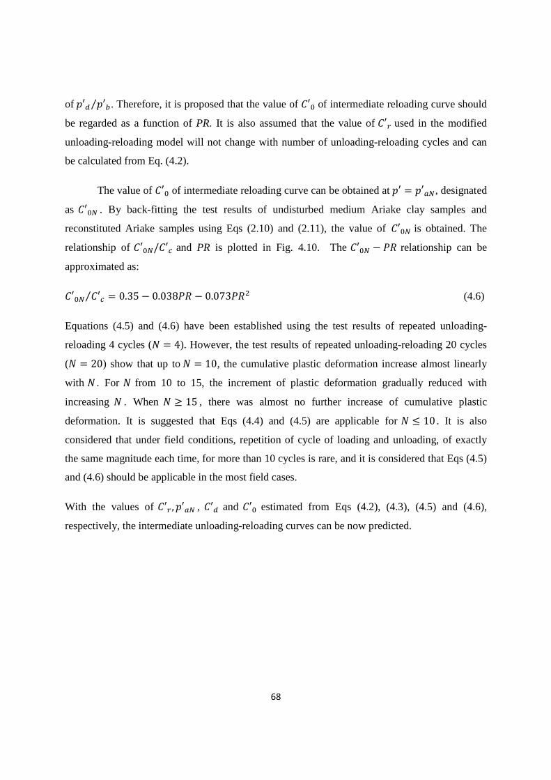
68

of′� ′�⁄ . Therefore, it is proposed that the value of #′� of intermediate reloading curve should

be regarded as a function of PR. It is also assumed that the value of #′) used in the modified

unloading-reloading model will not change with number of unloading-reloading cycles and can

be calculated from Eq. (4.2).

The value of #′� of intermediate reloading curve can be obtained at′ = ′�", designated

as#′�" . By back-fitting the test results of undisturbed medium Ariake clay samples and

reconstituted Ariake samples using Eqs (2.10) and (2.11), the value of #′�" is obtained. The

relationship of #′�"/#′� and PR is plotted in Fig. 4.10. The #′�" − %& relationship can be

approximated as:

#′�" #′�⁄ = 0.35 − 0.038%& − 0.073%&t (4.6)

Equations (4.5) and (4.6) have been established using the test results of repeated unloading-

reloading 4 cycles (� = 4). However, the test results of repeated unloading-reloading 20 cycles

(� = 20) show that up to� = 10, the cumulative plastic deformation increase almost linearly

with � . For � from 10 to 15, the increment of plastic deformation gradually reduced with

increasing� . When� ≥ 15 , there was almost no further increase of cumulative plastic

deformation. It is suggested that Eqs (4.4) and (4.5) are applicable for� ≤ 10 . It is also

considered that under field conditions, repetition of cycle of loading and unloading, of exactly

the same magnitude each time, for more than 10 cycles is rare, and it is considered that Eqs (4.5)

and (4.6) should be applicable in the most field cases.

With the values of#′) , ′�" , #′� and #′� estimated from Eqs (4.2), (4.3), (4.5) and (4.6),

respectively, the intermediate unloading-reloading curves can be now predicted.

69

p´d

p a = p aN

p´bN

vbNvb1

(b) vb1<vbN

p´b

log

v

log p'

C s

C d

C 0

C 0N

C C

p´b

p a

p d

C r

p aN

p´bN

vb1

vbN

(a) vb1>vbN

log

v

log p'

p c

Fig. 4.8 Illustration of changing ′� value: (a)�� > ��"; (b) �� < ��"

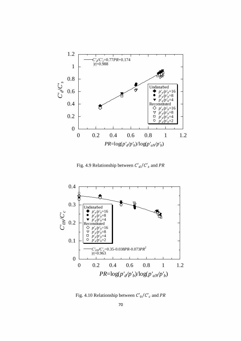
70

0 0.2 0.4 0.6 0.8 1 1.20

0.2

0.4

0.6

0.8

1

1.2C

' d/C

' s

PR=log(p'd/p'b)/log(p'aN/p'b)

Undisturbed p'a/p'b=16 p'a/p'b=8 p'a/p'b=4Reconstituted p'a/p'b=16 p'a/p'b=8 p'a/p'b=4 p'a/p'b=2

C'd/C's=0.77PR+0.174 |r|=0.988

Fig. 4.9 Relationship between #′� #′$⁄ and%&

0 0.2 0.4 0.6 0.8 1 1.20

0.1

0.2

0.3

0.4

C' 0N

/C' c

PR=log(p'd/p'b)/log(p'aN/p'b)

Undisturbed p'a/p'b=16p'a/p'b=8p'a/p'b=4

Reconstitutedp'a/p'b=16p'a/p'b=8p'a/p'b=4p'a/p'b=2

C'0N/C'c=0.35-0.038PR-0.073PR2

|r|=0.963

Fig. 4.10 Relationship between #′� #′�⁄ and%&

71

4.4 Simulation of laboratory test

4.4.1 Repeated intermediate unloading-reloading

For simulating the deformation of clayey soil samples induced by repeated intermediate

unloading-reloading by using modified unloading-reloading model, five model parameters i.e.,

#′� , #′$#′) , #′� and #′"� are required. The value of#′� and #′$ for simulating repeated

intermediate unloading-reloading cycles induced plastic deformation of undisturbed medium and

soft Ariake clay samples and reconstituted Ariake clay samples are given in Table 4.2. The

values of#′) ,, #′� and #′"� were estimated from Eqs (4.2), (4.5) and (4.6), respectively. The

change of ′� during repeated intermediate unloading-reloading cycles is also considered by

using Eq. (4.3). The repeated intermediate unloading-reloading curves of undisturbed medium

and soft Ariake clay samples and reconstituted Ariake clay samples were predicted and they are

compared with the measured soil responses in Figs 4.11 to 4.14. These predictions now fit the

test data well.

4.4.2 Small intermediate unloading-reloading

Base on the test results shown in Figs 3.11 and 3.12, deformation of reconstituted Ariake

samples was found to be profoundly influence by the small intermediate unloading-reloading

cycles. The modified model has been also used to predict the effect of small intermediate

reloading-unloading (r-u) and unloading-reloading (u-r) cycles for reconstituted Ariake clay

samples to check the applicability of the modified unloading-reloading model to this kind of

loading cycles. For Type I tests, followed a general unloading path and 3 tests conducted are: (i)

continuous unloading, (ii) one small intermediate r-u cycle and (iii) three small intermediate r-u

cycles. The values of #′� and #′$ were obtained from continuous unloading test as listed in Table

4.3. And for Type II tests followed a general reloading path and also involving 3 tests: (i)

continuous reloading, (ii) one small intermediate u-r cycle and (iii) four small intermediate u-r

cycles. The values of #′� and #′$ were obtained from continuous reloading test as also listed in

Table 4.3. The values of#′�, #′),#′� and #′�" were calculated from Eqs 4.1, 4.2, 4.5 and 4.6,

respectively. The simulated curves in log�� − log�� plot for Type I (general unloading) and

Type II (general reloading) tests are shown in Figs 4.15(b) and 4.16(b), respectively. For the test

results of general unloading combined with different number of small r-u cycles shown in Fig.

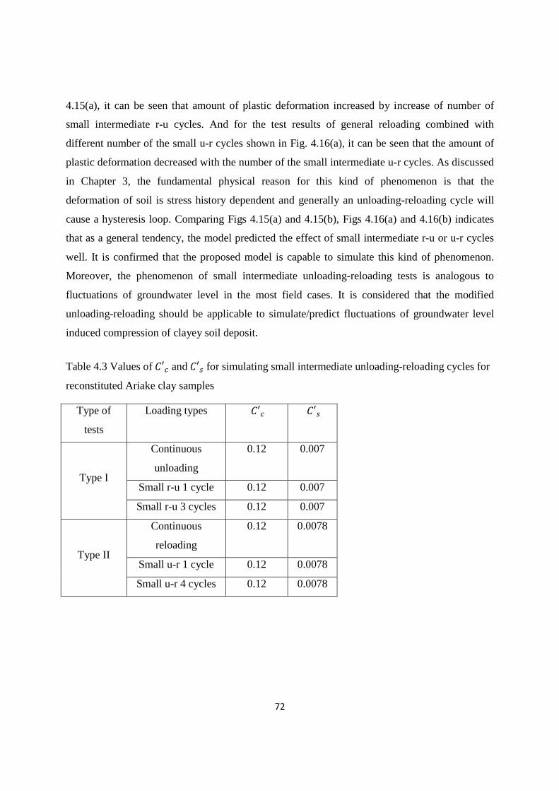
72

4.15(a), it can be seen that amount of plastic deformation increased by increase of number of

small intermediate r-u cycles. And for the test results of general reloading combined with

different number of the small u-r cycles shown in Fig. 4.16(a), it can be seen that the amount of

plastic deformation decreased with the number of the small intermediate u-r cycles. As discussed

in Chapter 3, the fundamental physical reason for this kind of phenomenon is that the

deformation of soil is stress history dependent and generally an unloading-reloading cycle will

cause a hysteresis loop. Comparing Figs 4.15(a) and 4.15(b), Figs 4.16(a) and 4.16(b) indicates

that as a general tendency, the model predicted the effect of small intermediate r-u or u-r cycles

well. It is confirmed that the proposed model is capable to simulate this kind of phenomenon.

Moreover, the phenomenon of small intermediate unloading-reloading tests is analogous to

fluctuations of groundwater level in the most field cases. It is considered that the modified

unloading-reloading should be applicable to simulate/predict fluctuations of groundwater level

induced compression of clayey soil deposit.

Table 4.3 Values of#′� and#′$ for simulating small intermediate unloading-reloading cycles for

reconstituted Ariake clay samples

Type of

tests

Loading types #′� #′$

Type I

Continuous

unloading

0.12 0.007

Small r-u 1 cycle 0.12 0.007

Small r-u 3 cycles 0.12 0.007

Type II

Continuous

reloading

0.12 0.0078

Small u-r 1 cycle 0.12 0.0078

Small u-r 4 cycles 0.12 0.0078

73

10 100 1000

2.1

2.2v

p' (kPa)

p'a/p'b=8p'd/p'b=8

Test Simulated

(a) p'b<p'd=p'a

10 100 10002.1

2.2

v

p' (kPa)

p'a/p'b=8p'd/p'b=4

Test Simulated

(b) p'b<p'd<p'a

p′a

p′b

p′d

p′a

p′b

Fig. 4.11 Measured and predicted intermediate unloading-reloading curves (medium Ariake

clay): (a)′� = ′�; (b) ′� < ′�

74

1 10 1003

3.1

3.2v

p' (kPa)

p'a/p'b=8p'd/p'b=8

test simulated

(a) p'd=p'a

1 10 1003

3.1

3.2

v

p' (kPa)

p'a/p'b=8p'd/p'b=4

test simulated

(b) p'd<p'a

p′a

p′b

p′d

p′a

p′b

Fig. 4.12 Measured and predicted intermediate unloading-reloading curves (reconstitued Ariake

clay): (a)′� = ′�; (b) ′� < ′�

75

1 10 100 10002.6

2.7

2.8

2.9

3

3.1

3.2

3.3

3.4

3.5

v

p' (kPa)

p'a/p'b=8p'd/p'b=8

Test Simulated

(a)

1 10 100 1000

3

3.1

3.2

v

p' (kPa)

p'a/p'b=8p'd/p'b=4

Test Simulated

(b)


(′� ′�⁄ = 8): (a)′� = ′�; (b) ′� < ′�

76

1 10 100 10002.5

2.6

2.7

2.8

2.9

v

p' (kPa)

p'a/p'b=4p'd/p'b=4

Test Simulated

(a)

10 100 10002.6

2.7

2.8

v

p' (kPa)

p'a/p'b=4p'd/p'b=2

Test Simulated

(b)


(′� ′�⁄ = 4): (a)′� = ′�; (b) ′� < ′�

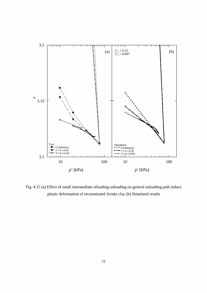
77

10 100

v

p' (kPa)

Simulation Continuous 1 r-u cycle 3 r-u cycles

(b)C'c = 0.12C's = 0.007

10 1003.1

3.2

(a)

Test Continuous 1 r-u cycle 3 r-u cycles

p' (kPa)

3.15

Fig. 4.15 (a) Effect of small intermediate reloading-unloading on general unloading path induce

plastic deformation of reconstituted Ariake clay (b) Simulated results

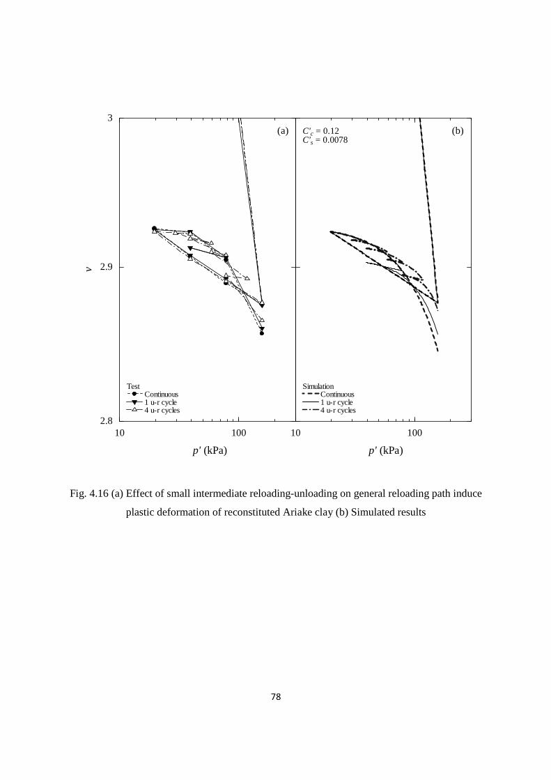
78

10 100

p' (kPa)

Simulation Continuous 1 u-r cycle 4 u-r cycles

(b)C'c = 0.12C's = 0.0078

10 1002.8

2.9

3

v

p' (kPa)

Test Continuous 1 u-r cycle 4 u-r cycles

(a)

Fig. 4.16 (a) Effect of small intermediate reloading-unloading on general reloading path induce

plastic deformation of reconstituted Ariake clay (b) Simulated results

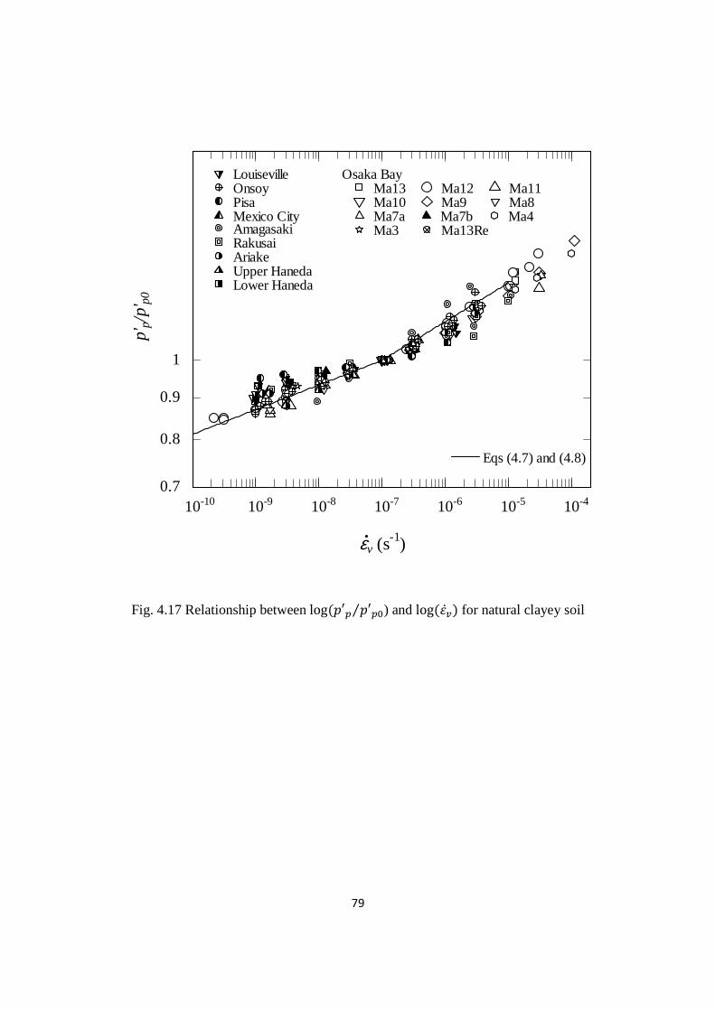
79

Fig. 4.17 Relationship betweenlog�′� ′��⁄ ) and log�� for natural clayey soil

10-10 10-9 10-8 10-7 10-6 10-5 10-40.7

0.8

0.9

1

Osaka Bay Ma13 Ma12 Ma11 Ma10 Ma9 Ma8 Ma7a Ma7b Ma4 Ma3 Ma13Re

p' p/

p'p0

εv (s-1)

AmagasakiRakusaiAriakeUpper HanedaLower Haneda

LouisevilleOnsoyPisaMexico City

Eqs (4.7) and (4.8)

80

4.5 Proposed method to determine yield stress with a known strain rate

One of the applications of the modified Butterfield model is in simulation of the land-

subsidence induced by groundwater level fluctuations. It is generally accepted that the yield

stress of a soft clayey deposit depends on strain rate (Leroueil 2006; Watabe et al. 2008; 2012).

Generally, the field strain rate is much smaller than that adopted in a standard laboratory

oedometer test (Leroueil 2006). The results of oedometer tests with a time interval between

successive loading increments of 1 day and 7 days in Chapter 3 (see Fig. 3.15) show clearly that

the yield stress is smaller for slow tests than for fast one.

Watabe et al. (2012) summarized the relationship between strain rate �� and normalized

yield stress,′�/′�� , where ′� is the measured yield stress and ′�� is the yield stress

corresponding to a strain rate of 1045 (s-1), for several clays in the world, as shown in Fig. 4.17.

Based on the data points plotted in Fig. 4.17, the experimental relationship can be approximated

by the following two equations:

ln i �fu�funk = 0.043ln�R ��T��TnW

�.5�; 104 �64 < �� < 104564 (4.7)

ln i �fu�funk = 0.043ln�R ��T��TnW

. �;104564 < �� < 104�64 (4.8)

where �� = 1045 (64 ).

For a standard laboratory oedometer test, the strain rate applied to a sample normally

depends on the compressibility and permeability of the soil and varies with both consolidation

pressure and elapsed time for a given load increment. As a rough approximation, Leroueil

(2006) estimated that the strain rate in a standard oedometer test is in the order of 1045(s-1). As

for the field strain rate, it varies widely and Leroueil (2006) estimated a typical range of 104w −104 �(s-1). This range is captured in Fig. 4.17 and, therefore, it is proposed that Eqs (4.7) and

(4.8) can be used to predict the yield stress for a known strain rate and known value of ′��.

81

4.6 Summary

This chapter presents the results of modeling unloading-reloading behaviour of clayey

soils, and comparison of simulated results with that of laboratory measured data, the following

summary can be drawn.

1) Butterfield’s unloading-reloading model (Butterfield 2011) can be used predict single unloading-reloading curves of the undisturbed soft and medium Ariake clay samples and reconstituted Ariake clay samples. Empirical methods have been established for evaluating the values of the model parameters, i.e. the initial slope of reloading curve, (#′)) and the slope at ’ = ′� (where ′� is the maximum consolidation pressure before unloading), (#′� ) of reloading path. However, the model cannot predict plastic deformation induced by repeated unloading-reloading cycles.

2) A model for predicting the one-dimensional deformation induced by repeated

unloading-reloading cycles has been proposed based on laboratory test results and the model

proposed by Butterfield (2011). The model has considered the change of the size yield locus due

to permanent volumetric strain caused by the repeated intermediate unloading-reloading cycles.

The maximum vertical effective stress before unloading (′�) was used to indicate the size of

yield locus, and a method to consider the change of ′� during repeated intermediate unloading-

reloading has been proposed. The method for evaluating the values of the model parameter have

been established, i.e. the slope of intermediate unloading curve, (#′�) for unloading path, and the

slope at = ′�" (where ′�" is the maximum vertical effective stress before intermediate

unloading), (#′�") and the initial slope of intermediate reloading curve, (#′)) for reloading path.

3) Comparing the results of simulated and measured of undisturbed medium and soft Ariake samples and reconstituted Ariake clay samples, indicates that the proposed unloading-reloading model is capable to simulate the effect of repeated intermediate unloading-reloading cycles.

4) Based on the data points plotted between strain rate �� and normalized yield stress,′�/′��, where ′� is the measured yield stress and ′�� is the yield stress corresponding

to a strain rate of 1045 (s-1), for several clays in the world reported by Watabe et al. (2012), the method to determine yield stress with a known strain rate has been proposed.

CHAPTER 5

APPLICATIONS TO FIELD CASE HISTORIES

5.1 Introduction

In this chapter, five case histories, i.e. two cases in Saga Plain, Japan (Ariake and

Shiroishi cases), one case in Yokohama, Japan and two cases in Bangkok Plain, Thailand

(Romaneenart Park and Kasetsart university campus cases) were analyzed and the results

presented. The modified unloading-reloading model has been used to simulate pore-water

variation induced compression of clayey soil layers of these sites. For two cases in Saga Plain,

the pore-water pressure variations in clayey soil layer were measured every hour. For Yokohama

and Bangkok cases, only monthly and weekly measured pore-water pressure data are available,

respectively. To investigate the effect of daily pore-water pressure variation on compression of

clayey soil layers of these cases, a daily pore-water variation pattern for 1 year period from

Ariake case has been produced and superposed to the measured general trade curves of the

Yakohama and Bangkok cases. The usefulness of the proposed unloading-reloading model is

discussed based on a comparison of the simulated and measured compression of the clayey soil

layers.

5.2 Simulating land-subsidence

Basic considerations

• Amount of pore-water pressure variations will be transferred to effective stress variations.

• Measured pore-water pressure variations at a monitoring point are applied to the soil

layer contains the monitoring point.

• Clayey soil layers are always saturated.

5.2.1 Two sites in Saga Plain, Japan

Saga Plain is located in the northwest of the Ariake Sea, Kyushu, Japan. In the plain,

there is a Holocene clayey soil deposit, known as Ariake clay, with a thickness of 10-30 m,

underlain by alternating Pleitocene sand and clay layers. The sites considered in this study are

located in the Shiroishi district and named as Ariake well site and Shiroishi well site. In the

84

Shiroishi district, due to excessive pumping of the groundwater for agricultural use, serious land-

subsidence occurred from the 1970s to 1990s (Miura et al. 1988; Sakai 2001). To control or at

least mitigate the rate of land-subsidence, the amount of groundwater being pumped has been

strictly regulated, and instead of groundwater, river water has been used for irrigation since 1995.

In the interim, there had been a tendency of groundwater level recovering. However, the

groundwater level still fluctuates seasonally or even daily, and land-subsidence has been still

observed. The phenomenon of fluctuating groundwater levels is analogous to repeated

intermediate unloading-reloading in an oedometer test, and therefore modified unloading-

reloading model has been used to simulate its effects.

(a) Ariake well site

The location of Ariake well is shown in Fig. 5.1. The groundwater level in each aquifer,

the compression of each soil layer, and the pore-water pressure in soft Ariake layers have been

monitored for about 7 years (Sakai 2001). A cross-sectional view of monitoring point at the

Ariake well site is shown in Fig. 5.2. In the soft clay layers, three pore-water pressure gauges

were installed at depths of 5.0, 10.0, and 21.0 m. In the Pleistocene aquifer located 26.0 m below

the ground surface, four observation wells have been installed at depths of 87.9, 80.5, 52.0, and

27.2 m to measure the groundwater level and the subsidence at each depth. Site investigation and

laboratory tests to determine soil properties at this site were conducted in 1996 (Sakai 2001), and

soil profiles and some soil properties are shown in Fig. 5.3. Fig. 5.5 shows the fluctuations of

pore-water pressure measured at 5.0, 10.0, and 21.0 m depth from the ground surface, from 1996

to 2003. The measuring time interval was 1 hour.

The initial conditions and the necessary parameters for using the proposed unloading-

reloading model are listed in Table 5.1. To calculate the compression of the soft clayey deposit,

the clayey layer was divided into 3 sub-layers. The boundaries between two adjacent sub-layers

were set at the middle between two adjacent pore-water pressure gauges. There is one pore-

water pressure gauge in each sub-layer and it was assumed that the measured pore-pressures

were the average values in that sub-layer. The values of #′� and #′$ were calculated from the

values of compression index (#�) and swelling index (#$) as:

#′� = 0.434#�/�1 + �� (5.1)

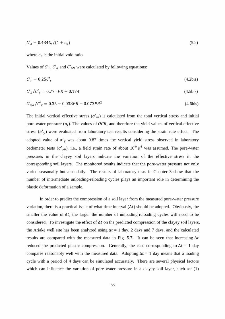
85

#′$ = 0.434#$/�1 + �� (5.2)

where �� is the initial void ratio.

Values of#′), #′� and #′�" were calculated by following equations:

#′) = 0.25#′$ (4.2bis)

#′� #′$⁄ = 0.77 ∙ %& + 0.174 (4.5bis)

#′�" #′�⁄ = 0.35 − 0.038%& − 0.073%&t (4.6bis)

The initial vertical effective stress (G′�9) is calculated from the total vertical stress and initial

pore-water pressure (<9). The values of1#&, and therefore the yield values of vertical effective

stress (G′7) were evaluated from laboratory test results considering the strain rate effect. The

adopted value of G′7 was about 0.87 times the vertical yield stress observed in laboratory

oedometer tests (G′7�), i.e., a field strain rate of about 10-9 s-1 was assumed. The pore-water

pressures in the clayey soil layers indicate the variation of the effective stress in the

corresponding soil layers. The monitored results indicate that the pore-water pressure not only

varied seasonally but also daily. The results of laboratory tests in Chapter 3 show that the

number of intermediate unloading-reloading cycles plays an important role in determining the

plastic deformation of a sample.

In order to predict the compression of a soil layer from the measured pore-water pressure

variation, there is a practical issue of what time interval (∆�) should be adopted. Obviously, the

smaller the value of∆�, the larger the number of unloading-reloading cycles will need to be

considered. To investigate the effect of ∆� on the predicted compression of the clayey soil layers,

the Ariake well site has been analyzed using ∆� = 1 day, 2 days and 7 days, and the calculated

results are compared with the measured data in Fig. 5.7. It can be seen that increasing ∆� reduced the predicted plastic compression. Generally, the case corresponding to ∆� = 1 day

compares reasonably well with the measured data. Adopting ∆� = 1 day means that a loading

cycle with a period of 4 days can be simulated accurately. There are several physical factors

which can influence the variation of pore water pressure in a clayey soil layer, such as: (1)

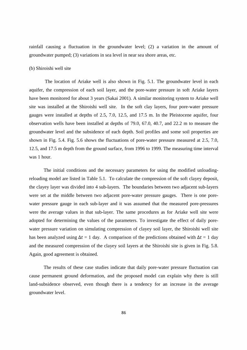
86

rainfall causing a fluctuation in the groundwater level; (2) a variation in the amount of

groundwater pumped; (3) variations in sea level in near sea shore areas, etc.

(b) Shiroishi well site

The location of Ariake well is also shown in Fig. 5.1. The groundwater level in each

aquifer, the compression of each soil layer, and the pore-water pressure in soft Ariake layers

have been monitored for about 3 years (Sakai 2001). A similar monitoring system to Ariake well

site was installed at the Shiroishi well site. In the soft clay layers, four pore-water pressure

gauges were installed at depths of 2.5, 7.0, 12.5, and 17.5 m. In the Pleistocene aquifer, four

observation wells have been installed at depths of 79.0, 67.0, 40.7, and 22.2 m to measure the

groundwater level and the subsidence of each depth. Soil profiles and some soil properties are

shown in Fig. 5.4. Fig. 5.6 shows the fluctuations of pore-water pressure measured at 2.5, 7.0,

12.5, and 17.5 m depth from the ground surface, from 1996 to 1999. The measuring time interval

was 1 hour.

The initial conditions and the necessary parameters for using the modified unloading-

reloading model are listed in Table 5.1. To calculate the compression of the soft clayey deposit,

the clayey layer was divided into 4 sub-layers. The boundaries between two adjacent sub-layers

were set at the middle between two adjacent pore-water pressure gauges. There is one pore-

water pressure gauge in each sub-layer and it was assumed that the measured pore-pressures

were the average values in that sub-layer. The same procedures as for Ariake well site were

adopted for determining the values of the parameters. To investigate the effect of daily pore-

water pressure variation on simulating compression of clayey soil layer, the Shiroishi well site

has been analyzed using ∆� = 1 day. A comparison of the predictions obtained with ∆� = 1 day

and the measured compression of the clayey soil layers at the Shiroishi site is given in Fig. 5.8.

Again, good agreement is obtained.

The results of these case studies indicate that daily pore-water pressure fluctuation can

cause permanent ground deformation, and the proposed model can explain why there is still

land-subsidence observed, even though there is a tendency for an increase in the average

groundwater level.

87

Fig. 5.1 Land-subsidence observation well points in Saga Plain

Fig. 5.2 Schematic view of observation points at Ariake well site

88

Fig. 5.3 Soil profile and physical and mechanical properties at Ariake well site

Fig. 5.4 Soil profile and physical and mechanical properties at Shiroishi well site

0 50 1000

10

20

30

40

50

60

Grain size (%)

<0.005 mm0.005-0.075 mm

>0.075 mm

0 100

wP wn wL

(%)

0 5 10 15

γd γt

(kN/m3)

0 1 2 3 4e0

0 500

Consolidationyield stress (kPa)

:OED :CRS

0 0.1 0.2Cs

0 1 2 3 4Cc

Dep

th (

G.L

.:m

)

Note:wn=water content, wp=plastic limit, wL=liquid limit, γd=dry unit weight γt=total unit weight, e0=initial void ratio, Cc=compression index, Cs=swelling index

0 50 1000

10

20

30

40

50

60

70

80

Grain size (%)

<0.005 mm0.005-0.075 mm

>0.075 mm

0 100

wP wn wL

(%)

0 5 10 15

γd γt

(kN/m3)

0 1 2 3 4e0

0 5001000


:OED :CRS

0 0.1 0.2Cs

0 1 2 3 4Cc

De

pth

(G

.L.:

m)

Note:wn=water content, wp=plastic limit, wL=liquid limit, γd=dry unit weight γt=total unit weight, e0=initial void ratio, Cc=compression index, Cs=swelling index

89

Table 5.1 Initial conditions and parameters used in analysis for Ariake and Shiroishi sites

Depth and

symbols Ariake well Shiroishi well

Depth (m) 0-7.5 7.5-15.5 15.5-27.2 0-5.0 5.0-10.0 10.0-15.0 15.0-22.5

<9 (kPa) 28.5 74.56 177.56 19.62 59.84 97.12 135.39

G′�9 (kPa) 19.36 72.07 109.81 12.26 37.03 66.02 116.18

G′7� (kPa) 50.00 85.00 145.00 26.00 62.00 91.00 147.00

G′7 (kPa) 43.50 73.95 126.15 22.62 53.94 79.17 127.89

�� 3.8 3.0 2.0 4.4 3.5 2.9 2.0

#′� 0.163 0.152 0.188 0.163 0.145 0.154 0.106

#′$ 0.0163 0.0152 0.0188 0.0189 0.0169 0.0145 0.0116

#′) 0.0041 0.0038 0.0047 0.0047 0.0042 0.0036 0.0029

90

0 500 1000 1500 2000 250020

30

40

time (days)

Por

e-w

ate

r pr

ess

ure

(kP

a) -5 m depth

0 500 1000 1500 2000 250070

75

80

85

-10 m depth

0 500 1000 1500 2000 2500160

170

180

190

200

-21 m depth

6/1/1996 3/31/2003

Fig. 5.5 Variations of pore-water pressure in clayey layers at Ariake well site

91

0 200 400 600 800 100010

20

30

time (days)

Po

re-w

ate

r p

ress

ure

(kP

a)

-2.5 m depth

6/1/1996

0 200 400 600 800 100055

60

65

70

75

-7 m depth

0 200 400 600 800 100090

100

110

-12.5 m depth

0 200 400 600 800 1000120

130

140

150

160

-17.5 m depth

2/26/1999

Fig. 5.6 Variations of pore-water pressure in clayey layers at Shiroishi well site

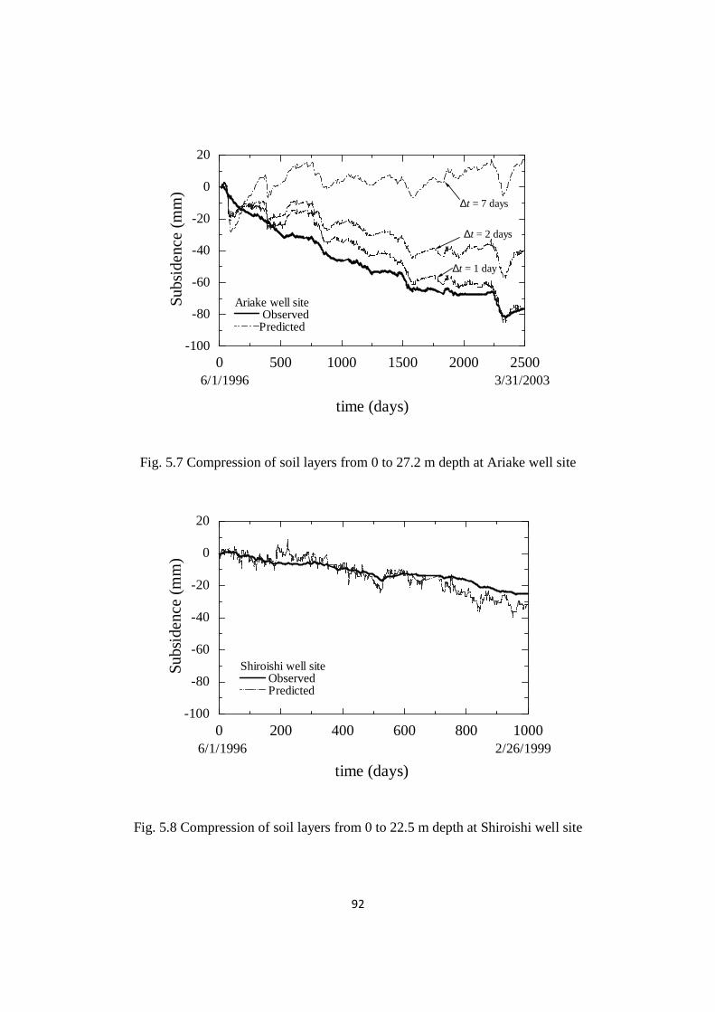
92

Fig. 5.7 Compression of soil layers from 0 to 27.2 m depth at Ariake well site

Fig. 5.8 Compression of soil layers from 0 to 22.5 m depth at Shiroishi well site

0 500 1000 1500 2000 2500-100

-80

-60

-40

-20

0

20

time (days)

Sub

side

nce

(m

m)

Ariake well site ObservedPredicted

6/1/1996 3/31/2003

∆t = 1 day

∆t = 2 days

∆t = 7 days

0 200 400 600 800 1000-100

-80

-60

-40

-20

0

20

time (days)

Su

bsid

en

ce (

mm

)

Shiroishi well site Observed Predicted

6/1/1996 2/26/1999

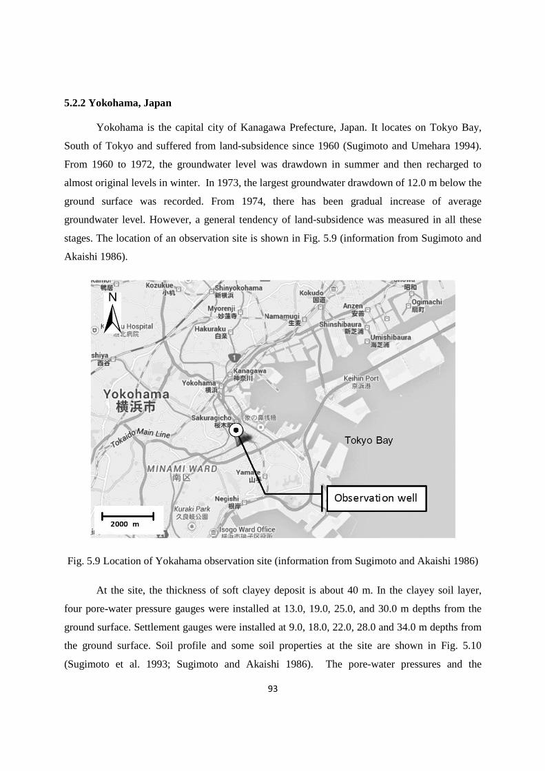
93

5.2.2 Yokohama, Japan

Yokohama is the capital city of Kanagawa Prefecture, Japan. It locates on Tokyo Bay,

South of Tokyo and suffered from land-subsidence since 1960 (Sugimoto and Umehara 1994).

From 1960 to 1972, the groundwater level was drawdown in summer and then recharged to

almost original levels in winter. In 1973, the largest groundwater drawdown of 12.0 m below the

ground surface was recorded. From 1974, there has been gradual increase of average

groundwater level. However, a general tendency of land-subsidence was measured in all these

stages. The location of an observation site is shown in Fig. 5.9 (information from Sugimoto and

Akaishi 1986).

Fig. 5.9 Location of Yokahama observation site (information from Sugimoto and Akaishi 1986)

At the site, the thickness of soft clayey deposit is about 40 m. In the clayey soil layer,

four pore-water pressure gauges were installed at 13.0, 19.0, 25.0, and 30.0 m depths from the

ground surface. Settlement gauges were installed at 9.0, 18.0, 22.0, 28.0 and 34.0 m depths from

the ground surface. Soil profile and some soil properties at the site are shown in Fig. 5.10

(Sugimoto et al. 1993; Sugimoto and Akaishi 1986). The pore-water pressures and the

94

compressions of soil layers were monitored with about 1 month interval for about 4 years from

1988 to 1993 (Sugimoto and Umehara 1994). For the purpose of settlement calculation, the

clayey soil layer is divided into 4 sub-layers with the depth of the settlement gauge as dividing

line as shown in Fig. 5.11.

Fig. 5.10 Soil profile and some physical and mechanical properties at Yokohama location

(Sugimoto et al. 1993; Sugimoto and Akaishi 1986)

0

10

20

30

40

F

AP

AC2

AC2

Dep

th (

m)

Note: F=backfill, AP=peat, AC=clay; wn=water content, γt=total unit weight, Cc=compression index

0 50 100wn (%)

AC1

10 15γt (kN/m3)

0 200


0 1 2CcSoil profile

95

-18.0 m

-28.0 m

-34.0 m

-22.0 m

Piezometer

-13.0 m

-19.0 m

-25.0 m

-30.0 m

Layer I

Layer II

Layer III

Layer IV

-9.0 m

0.0 m

Settlement gauge

Fig. 5.11 Location of piezometer and settlement gauge at Yokohama site

In this way the calculated compressions can be directly compared with the measured data. The

modified unloading-reloading model was used to simulate pore-water pressure variation induced

compression of each soil layer. The initial conditions and the necessary parameters for using the

model are listed in Table 5.2. The same procedures as for the cases in Saga Plain were used for

determining the values of the parameters. The measured pore-water pressures are shown in Fig.

5.12.

96

Fig. 5.12 Measured pore-water pressure at Yokohama site

0 400 800 1200 160090

100

110

120

time (days)

Por

e-w

ate

r p

ress

ure

(kP

a)

-13.0 m depth

12/1988

(a)

0 400 800 1200 1600160

170

180

190-19.0 m depth

(b)

0 400 800 1200 1600210

220

230

240-25.0 m depth

(c)

0 400 800 1200 1600250

260

270

280-30.0 m depth

5/1993

(d)

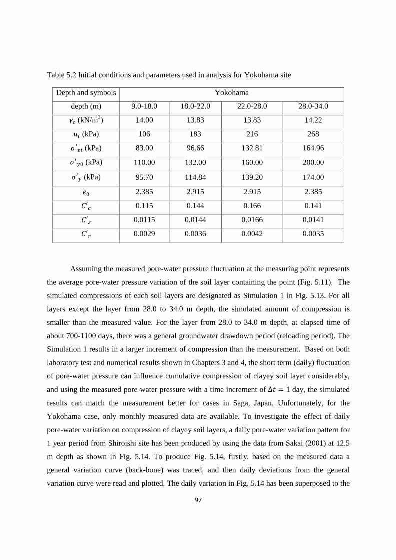
97

Table 5.2 Initial conditions and parameters used in analysis for Yokohama site

Depth and symbols Yokohama

depth (m) 9.0-18.0 18.0-22.0 22.0-28.0 28.0-34.0

DE (kN/m3) 14.00 13.83 13.83 14.22

<9 (kPa) 106 183 216 268

G′�9 (kPa) 83.00 96.66 132.81 164.96

G′7� (kPa) 110.00 132.00 160.00 200.00

G′7 (kPa) 95.70 114.84 139.20 174.00

�� 2.385 2.915 2.915 2.385

#′� 0.115 0.144 0.166 0.141

#′$ 0.0115 0.0144 0.0166 0.0141

#′) 0.0029 0.0036 0.0042 0.0035

Assuming the measured pore-water pressure fluctuation at the measuring point represents

the average pore-water pressure variation of the soil layer containing the point (Fig. 5.11). The

simulated compressions of each soil layers are designated as Simulation 1 in Fig. 5.13. For all

layers except the layer from 28.0 to 34.0 m depth, the simulated amount of compression is

smaller than the measured value. For the layer from 28.0 to 34.0 m depth, at elapsed time of

about 700-1100 days, there was a general groundwater drawdown period (reloading period). The

Simulation 1 results in a larger increment of compression than the measurement. Based on both

laboratory test and numerical results shown in Chapters 3 and 4, the short term (daily) fluctuation

of pore-water pressure can influence cumulative compression of clayey soil layer considerably,

and using the measured pore-water pressure with a time increment of ∆� = 1 day, the simulated

results can match the measurement better for cases in Saga, Japan. Unfortunately, for the

Yokohama case, only monthly measured data are available. To investigate the effect of daily

pore-water variation on compression of clayey soil layers, a daily pore-water variation pattern for

1 year period from Shiroishi site has been produced by using the data from Sakai (2001) at 12.5

m depth as shown in Fig. 5.14. To produce Fig. 5.14, firstly, based on the measured data a

general variation curve (back-bone) was traced, and then daily deviations from the general

variation curve were read and plotted. The daily variation in Fig. 5.14 has been superposed to the

98

general trade curve of the Yokohama measured data as shown in Fig. 5.15. It is understood that

the pore-water pressure variation in Saga may (or most likely) not represent the true situation in

Yokohama, and the purpose of this kind estimation is to investigate the effect of small

intermediate unloading-reloading cycles on simulated permanent deformation. Using the pore-

water pressure variations of solid line in Fig. 5.15, the simulated compressions of clayey layer at

Yokohama site (Simulation 2) are compared in Fig. 5.16. It can be seen that for all layers

Simulation 2 yielded a better result when compared with the measured data. There are two points

need to be emphasized. In Fig. 5.15(c), for the elapsed time from about 200 to 600 days, there is

a general trade of increase pore-water pressure (<) (unloading). When considering the assumed

daily pore-water pressure variation, the simulated compression is larger (Fig. 5.16(c)). This

phenomenon is similar to the laboratory test results of a general unloading path combined with

small intermediate reloading-unloading (r-u) cycles (see Fig. 3.11). The results show that small

intermediate r-u cycles on a general unloading path can induce plastic strain increment. While in

Fig. 5.15(d) from about 700 to 1100 days of the elapsed time, there is a general trade of pore-

water pressure reduction (reloading). In this case, considering the assumed small intermediate

pore-water pressure variation resulted in a smaller simulated compression, and which is closer to

the measured data (Fig. 5.16(d)). This phenomenon is similar to the laboratory test results of a

general reloading path combined with small intermediate unloading-reloading (u-r) cycles (see

Fig. 3.12). The results show that small intermediate u-r cycles on a general reloading path cause

smaller plastic deformation. These calculations clearly indicate that to simulate/predict

compression of clayey soil layer due to groundwater level variation, daily pore-water pressure

measurement is necessary.

99

Fig. 5.13 Measured and simulated compressions of clayey soil layers at Yokohama site

0 400 800 1200 1600-15

-10

-5

0

5

time (days)

Am

ount

of c

omp

ress

ion

(mm

)9.0-18.0 m depth

12/1988

(a)

0 400 800 1200 1600-15

-10

-5

0

518.0-22.0 m depth

(b)

0 400 800 1200 1600-15

-10

-5

0

5

1022.0-28.0 m depth(c)

0 400 800 1200 1600-15

-10

-5

0

528.0-34.0 m depth

5/1993

Measured Simulation 1

(d)

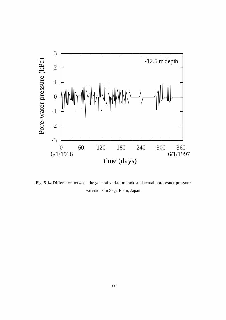
100

0 60 120 180 240 300 360-3

-2

-1

0

1

2

3-12.5 m depth

Por

e-w

ate

r p

ress

ure

(kP

a)

time (days)6/1/1996 6/1/1997

Fig. 5.14 Difference between the general variation trade and actual pore-water pressure

variations in Saga Plain, Japan

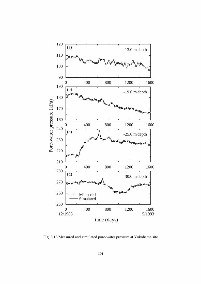
101

0 400 800 1200 160090

100

110

120

time (days)

Por

e-w

ate

r pr

ess

ure

(kP

a)

-13.0 m depth

12/1988

(a)

0 400 800 1200 1600160

170

180

190-19.0 m depth

(b)

0 400 800 1200 1600210

220

230

240-25.0 m depth

(c)

0 400 800 1200 1600250

260

270

280-30.0 m depth

5/1993

Measured Simulated

(d)

Fig. 5.15 Measured and simulated pore-water pressure at Yokohama site

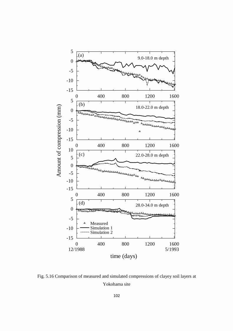
102

0 400 800 1200 1600-15

-10

-5

0

5

time (days)

Am

ount

of c

ompr

ess

ion

(mm

)9.0-18.0 m depth

12/1988

(a)

0 400 800 1200 1600-15

-10

-5

0

518.0-22.0 m depth

(b)

0 400 800 1200 1600-15

-10

-5

0

5

1022.0-28.0 m depth(c)

0 400 800 1200 1600-15

-10

-5

0

528.0-34.0 m depth

5/1993

Measured Simulation 1 Simulation 2

(d)

Fig. 5.16 Comparison of measured and simulated compressions of clayey soil layers at

Yokohama site

103

5.2.3 Two sites in Bangkok, Thailand

Bangkok Plain lies between Ayutthaya and the Gulf of Thailand. In the plain deposited a

thick marine clay layer up to 30 m thick, known as the Bangkok clay. The upper 15 m of

Bangkok clay, called the soft Bangkok clay, is very soft and highly compressible. The lower part,

known as stiff Bangkok clay extends to an average depth of 25 to 30 m, underlain by alternating

sand and clay layers. Soil strata in Bangkok Plain consist of 8 main aquifers (Giao et al. 2012).

The upper four aquifers in 200 m deep zone are the Bangkok (BK) aquifer (~50 m depth); the

Phra Pradaeng (PD) aquifer (~100 m depth); Nakorn Laung (NL) aquifer (~150 m depth) and

Nonthaburi (NB) aquifer (~200 m depth). Most wells in Bangkok were drilled into these aquifers.

A large-scale extraction of groundwater from the aquifer system started in early 1950s and land-

subsidence was observed (Phien-wej et al. 2006). Groundwater over-pumping in the 1970-1980s

led to a drastic drawdown in piezometric head of up to 40-50 m in the NL and NB aquifers. Due

to government regulation, from the middle of 1990s, the groundwater level in the aquifers was

recovered (Giao et al. 2012; Fornes and Pirarai 2014). However, a general tendency of

permanent compression of soft clayey deposit was still measured. The sites considered in

Bangkok area are located in Romaneenart Park and Kasetsart University campus, Bangkok.

(a) Romaneenart Park site

At the Romaneenart Park site the thickness of soft clayey deposit is about 14 m. In soft

clayey layer, a pore-water pressure gauge was installed at 10.0 m depth from the ground surface.

The compression of soft clay layer was monitored from 0 to 14.77 m depth. Base on the data

reported by Department of Ground Water Resource (Seven Associated Consultants Co., Ltd.

2012), the soil profile with some physical and mechanical properties at the monitoring site are

given in Figs 5.17. The weekly measured pore-water pressures and compressions of the clayey

soil layer are shown in Figs 5.20 and 5.22, respectively. The same procedures as for the cases in

Saga Plain were used for determining the values of the parameters. The daily pore-water pressure

variation from Saga Plain in Fig. 5.14 was also superposed on the measured pore-water pressure

at Bangkok site and the resulting pore-water pressure variations are shown in Fig. 5.20 as solid

line. The simulated compressions using weekly measured and assumed daily varied pore-water

pressure are designated as Simulation 1 and Simulation 2 and compared with the measured data

in Fig. 5.22, respectively. For this case, there is a general pore-water pressure reduction period

104

(reloading) at the beginning for about 2 months. It can be clearly seen that considering small

intermediate u-r cycles can result in smaller simulated permanent deformation of clayey layer

which is closer to the measured data.

(b) Kasetsart University campus site

At the Kasetsart University campus site the thickness of soft clayey deposit is about 13

m. In soft clayey layer, two pore-water pressure gauges were installed at 4.68 and 8.65 m depth

from the ground surface. The compression of soft clay layer was monitored from 0 to 12.08 m

depth. Soil profile with some physical and mechanical properties at the monitoring site is given

in Figs 5.18 (Seven Associated Consultants Co., Ltd. 2012). To calculate the compression of the

soft clayey deposit, the clayey layer was divided into 2 sub-layers as shown in Fig. 5.19. The

boundary between sub-layer was set at the middle between two pore-water pressure gauges.

There is one pore-water pressure gauge in each sub-layer and it was assumed that the measured

pore-water pressures were the average values of that sub layer. The weekly measured pore-water

pressures and compressions of the clayey soil layer are shown in Figs 5.21 and 5.23, respectively.

The initial conditions and the necessary parameters are listed in Table 5.4. The same procedures

as Saga Plain cases used for determining the values of the parameters. The daily pore-water

pressure variation from Saga Plain in Fig. 5.14 was superposed on the measured pore-water

pressure at Kasetsart University campus site and the resulting pore-water pressure variations are

shown in Fig. 5.21 as solid line. Using the measured and assumed pore-water pressure variations

of solid line in Fig. 5.21, the simulated compressions of clayey layer designated as Simulation 1

and Simulation 2 are compared with the measured data in Fig. 5.23, respectively. It can be seen

that the simulated amount of compression using the assumed pore-water pressure (Simulation 2)

is larger than the measured value (Simulation 1) and Simulation 2 yielded a better result when

compared with the measured data.

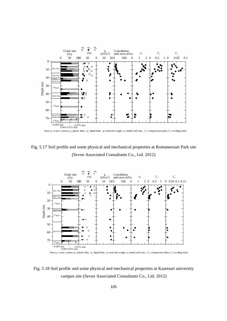
105

Fig. 5.17 Soil profile and some physical and mechanical properties at Romaneenart Park site

(Seven Associated Consultants Co., Ltd. 2012)

Fig. 5.18 Soil profile and some physical and mechanical properties at Kasetsart university

campus site (Seven Associated Consultants Co., Ltd. 2012)

0 50 100

Grain size (%)

<0.005 mm0.005-0.075 mm

>0.075 mm

0 50

wP wn wL

(%)

0 10 20

γt(kN/m3)

0 1 2

e0

0 500


0 0.05 0.1

Cs

0 0.5 1

Cc

Dep

th (

m)

0

10

20

30

40

50

60

70

Soft Clay

Stiff Clay

1stSand

Hard Clay

2ndSand

3rdSand

Hard Clay

4thSand

Hard Clay

Note:wn=water content, wp=plastic limit, wL=liquid limit, γt=total unit weight, e0=initial void ratio, Cc=compression index, Cs=swelling index

0 50 100

Grain size (%)

<0.005 mm0.005-0.075 mm

>0.075 mm

0 50

wP wn wL (%)

0 10 20

γt(kN/m3)

0 1 2

e0

0 500


0 0.050.1 0.15

Cs

0 0.5 1

Cc

Dep

th (

m)

0

10

20

30

40

50

60

70

Soft Clay

Stiff Clay

1stSand

Hard Clay

2ndSand

3rdSand

Hard Clay

Note:wn=water content, wp=plastic limit, wL=liquid limit, γt=total unit weight, e0=initial void ratio, Cc=compression index, Cs=swelling index

106

Fig. 5.19 Location of piezometer and settlement gauge at Kasetsart University campus site

Table 5.3 Initial conditions and parameters used in analysis for Romneenart Park site

Depth and symbols Romneenart Park

depth (m) 0-14.77

DE (kN/m3) 16.1

<9 (kPa) 78.50

G′�9 (kPa) 40.40

G′7� (kPa) 90.73

G′7 (kPa) 78.93

�� 1.7

#′� 0.105

#′$ 0.0059

#′) 0.0015

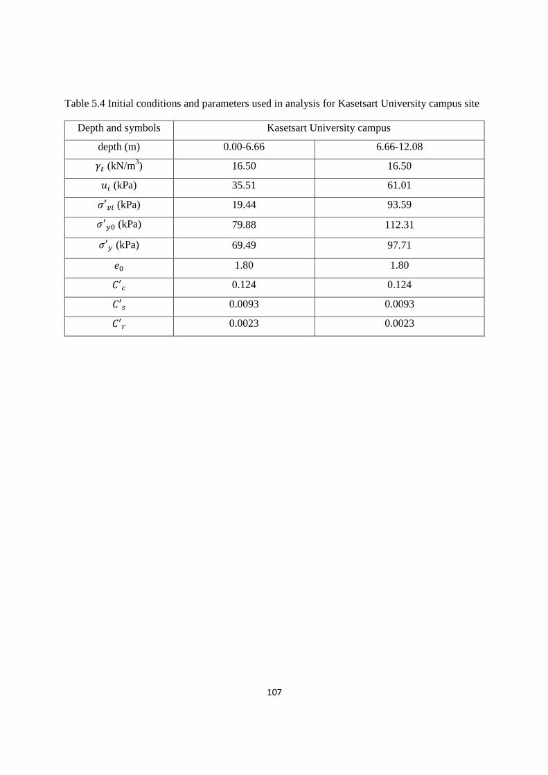
107

Table 5.4 Initial conditions and parameters used in analysis for Kasetsart University campus site

Depth and symbols Kasetsart University campus

depth (m) 0.00-6.66 6.66-12.08

DE (kN/m3) 16.50 16.50

<9 (kPa) 35.51 61.01

G′�9 (kPa) 19.44 93.59

G′7� (kPa) 79.88 112.31

G′7 (kPa) 69.49 97.71

�� 1.80 1.80

#′� 0.124 0.124

#′$ 0.0093 0.0093

#′) 0.0023 0.0023

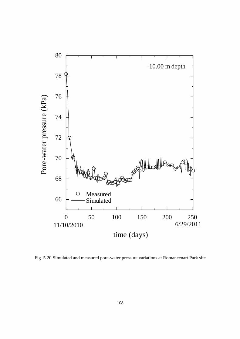
108

0 50 100 150 200 250

66

68

70

72

74

76

78

80

time (days)

Po

re-w

ate

r pr

ess

ure

(kP

a)

-10.00 m depth

11/10/2010 6/29/2011

Measured Simulated

Fig. 5.20 Simulated and measured pore-water pressure variations at Romaneenart Park site

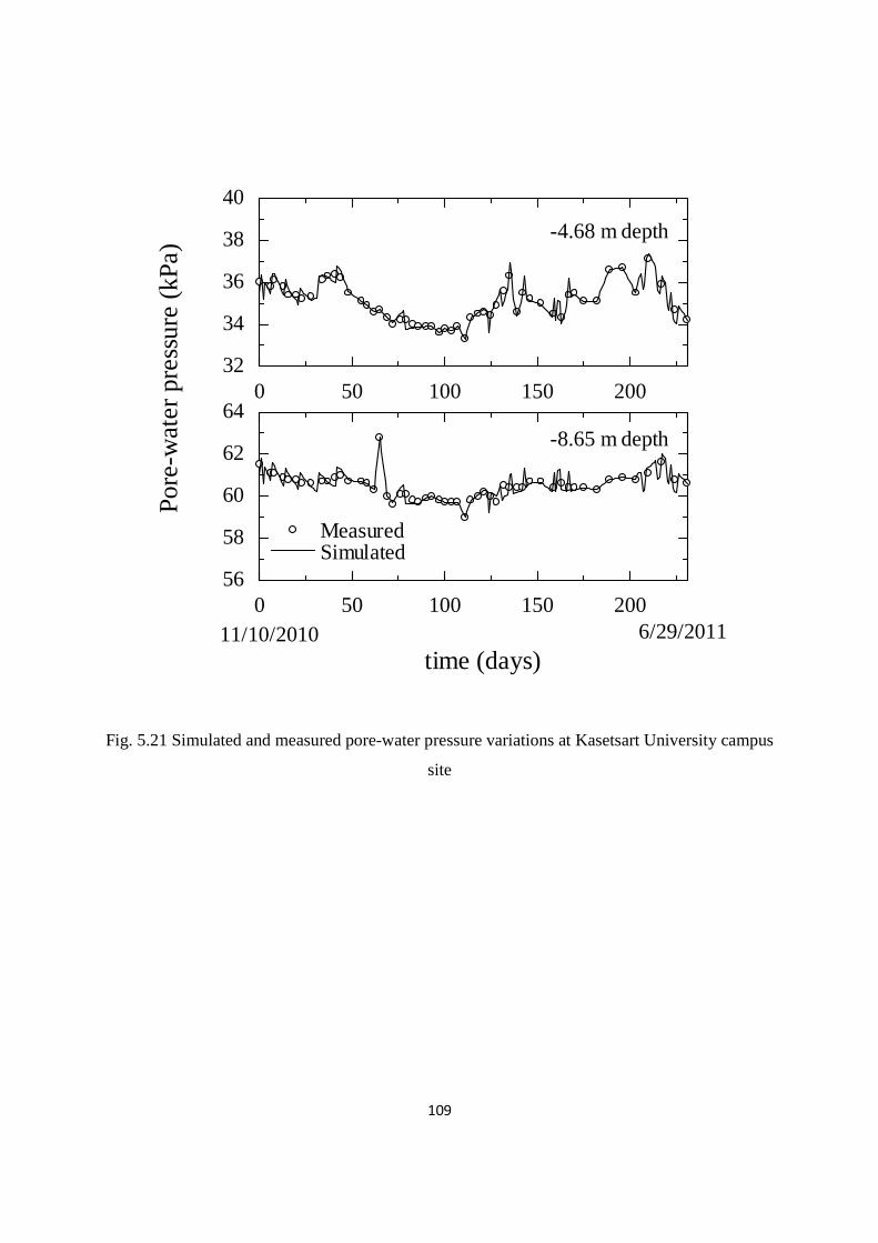
109

Fig. 5.21 Simulated and measured pore-water pressure variations at Kasetsart University campus

site

0 50 100 150 20032

34

36

38

40

time (days)

Por

e-w

ate

r pr

ess

ure

(kP

a)

-4.68 m depth

11/10/2010 6/29/2011

Measured Simulated

0 50 100 150 20056

58

60

62

64-8.65 m depth

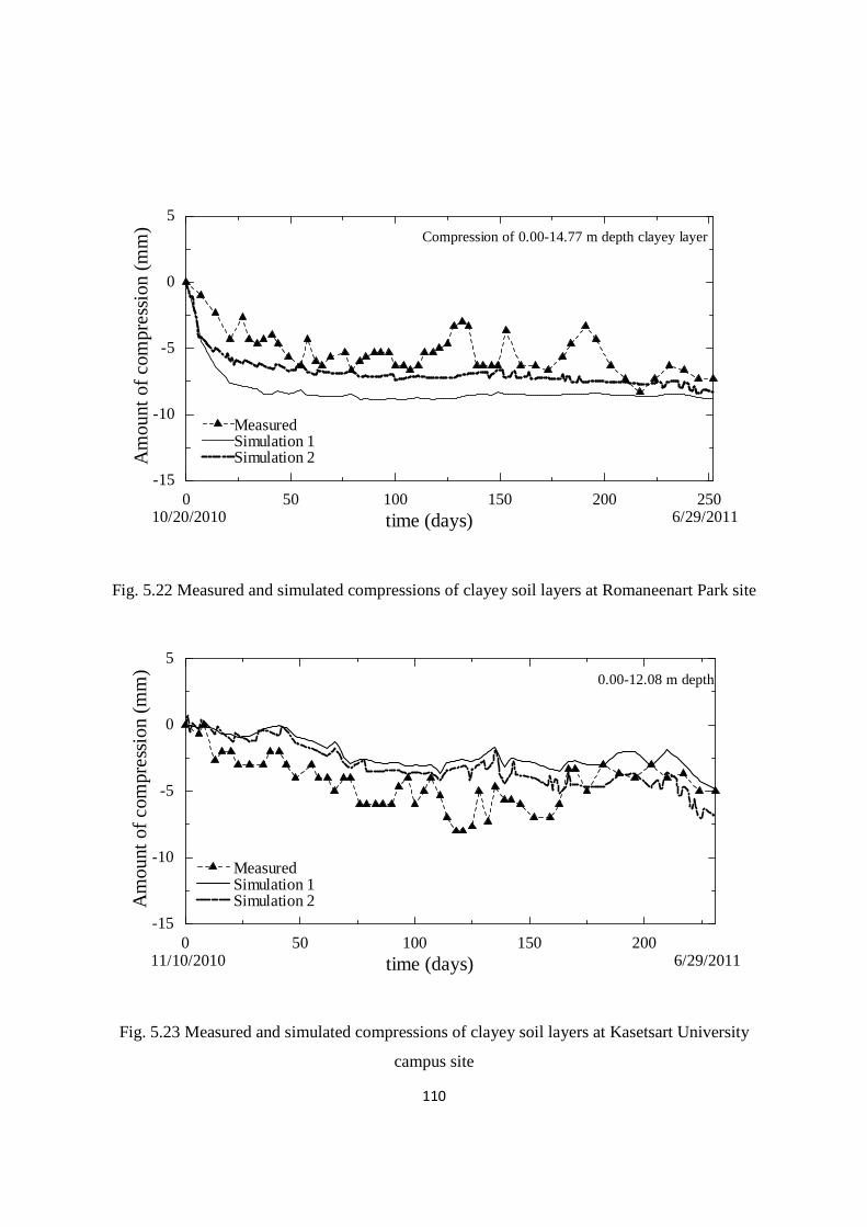
110

0 50 100 150 200 250-15

-10

-5

0

5

time (days)

Am

ount

of c

ompr

ess

ion

(m

m)

Compression of 0.00-14.77 m depth clayey layer

10/20/2010 6/29/2011


Fig. 5.22 Measured and simulated compressions of clayey soil layers at Romaneenart Park site

Fig. 5.23 Measured and simulated compressions of clayey soil layers at Kasetsart University

campus site

0 50 100 150 200-15

-10

-5

0

5

time (days)

Am

ount

of c

ompr

ess

ion

(mm

)

0.00-12.08 m depth

11/10/2010 6/29/2011


111

5.3 Summary

Compression of clayey soil deposit induce by fluctuations of pore-water pressure of five

case histories, i.e. two cases in Saga Plain, Japan; one case in Yokohama, Japan; and two cases in

Bangkok, Thailand, have been simulated by using a proposed unloading-reloading model; the

following summary can be made.

1). For Saga Plain cases where real time pore-water pressure monitoring was made with a

time interval 1 hour, good agreement was obtained between the simulated and field measured

values using a time increment for considering groundwater level variation of∆� = 1 day.

2) For Yokohama and Bangkok cases where the time intervals for pore-water pressure

measurement was about one month and one week respectively. To investigate the effect of daily

pore-water pressure variation on compression of clayey soil layers, a daily pore-water variation

pattern for 1 year period from one case in Saga Plain has been produced and then superposed to

the measured general trade curve of Yokohama and Bangkok sites. The simulated results

between measured and assumed pore-water pressure variation were compared with the field

measured of compression. It can be seen that for a general trade of pore-water pressure increase,

the assumed pore-water pressure variation resulted in a larger simulated compression, which is

closer to the measured compression data. And for a general trade of pore-water reduction, the

assumed pore-water pressure variation resulted in a smaller simulated compression, which is also

closer to the measured compression data. Therefore, it has been demonstrated that to correctly

simulate/predict groundwater level variation induce compression (settlement) of clayey soil

layers, considering daily pore-water pressure variation is necessary.

CHAPTER 6

CONCLUDING REMARKS

6.1 Conclusions

This study mainly investigates the effect of intermediate unloading-reloading on one-

dimensional deformation behaviour of clayey soil samples. A series of laboratory oedometer

tests were conducted. And based on the test results, a suitable model for predicting the

deformation behaviour of clayey deposit under repeated unloading-reloading cycles has been

proposed. Then the model was applied to simulate the effect of pore-water pressure variations

induced compression of clayey soil deposits at 5 sites in Japan and Thailand. Based on the results

of the laboratory tests and analysis, the following conclusions can be drawn.

(1) Deformation behaviour of clay under repeated intermediate unloading-reloading

a) Under oedometer condition, unloading curve is close to linear in log�� − log�� (� = 1 + �, and � is the void ratio, and ′ is the consolidation stress) plot, but reloading curve is

non-linear. Even in overconsolidated region, repeated unloading-reloading will induce plastic

deformation. For reconstituted sample, with a given range of stress change up to 10 unloading-

reloading cycles, the plastic deformation increased almost linearly with the increase of number of

the cycles. However, for microstructured undisturbed sample, when intermediate unloading

pressure (′� ) is the same pressure as the maximum vertical effective stress before the first

unloading (′�), increment of plastic deformation decreased drastically with the increase of the

number of unloading-reloading cycle (�) for � = 1 to 4 due to the destructuring effect.

b) Under oedometer condition, for a general unloading path, small intermediate

reloading-unloading (r-u) cycles caused increase of the final plastic deformation. And for a

general reloading path, small intermediate unloading-reloading (u-r) cycles caused reduction of

the final plastic deformation.

c) The results of oedometer test with a time interval between successive loading

increments of 1 day and 7 days indicate that the yield stress was smaller for the longer time

114

interval. It is considered that strain rate is lower for 7 days interval test than that for 1 day

interval test.

(2) Predicting unloading-reloading induced plastic deformation

a) A model proposed by Butterfield (2011) has been used to simulate deformation of

unloading-reloading cycle of clayey soil samples. Methods have been established for evaluating

the values of the model parameters. Comparing the simulated and measured results indicates that

the model can simulate single unloading-reloading curves well. However, since the model

assumed that deformation of clay under repeated intermediate unloading-reloading cycle is

purely elastic, the model fails to simulate plastic deformation induced by repeated intermediate

unloading-reloading cycles.

b) A new model for predicting the deformation of clay induced by repeated unloading-

reloading cycles under oedometer condition has been proposed. The model considers the change

of the maximum vertical effective stress before unloading (′�) during repeated intermediate

unloading-reloading induced plastic volumetric strain. Method for evaluating the values of the

model parameter has been established.

c) Comparing the results of simulated and measured indicates that the proposed

unloading-reloading model is capable to simulate the effect of repeated intermediate unloading-

reloading cycles.

(3) Application of the proposed model to the field case histories

a) The proposed model has been used to simulate the daily fluctuations in groundwater

pressure induced compression of soft clayey deposit in Saga Plain, Japan where real time pore-

water pressure monitoring was made with a time interval of 1 hour. Good agreement was

obtained between the simulated and field measured values.

b) Other three case histories analyzed are in Yokohama, Japan and in Bangkok, Thailand,

where the time intervals for pore-water pressure measurement was about one month and one

week, respectively, while the analysis using an assumed daily variation of pore-water pressure

was also conducted for comparison. Comparing with the field measured of settlement, it has been

115

demonstrated that to correctly simulate/predict groundwater pressure variation induce

compression (settlement) of clayey soil layers, considering daily pore-water pressure variation is

necessary.

6.2 Recommendation for future works

(1) In this study, the daily pore-water pressure used for calculating vertical effective

stress is obtained from monitored data in the clayey soil layer at the site. However, for many

field cases, the monitored data of daily pore-water pressure variation in clayey soil is not

available, and only the fluctuation of groundwater pressure in the aquifer was monitored. If a

method for linking pore-water pressure variation in aquifer to that in clayey soil layers can be

established, the method proposed in this study can be applied to those cases. Further study on

this aspect is recommended.

(2) Most of laboratory tests conducted in this study had a time interval between two

loading steps of 1 day. Only one test had a time interval 7 days. Further experimental

investigation on the effect of time interval on the deformation behaviour of clayey soil samples is

required.

REFFERENCES

ASTM. (2006). Standard practice for classification of soils for engineering purposes (Unified

Soil Classification System). ASTM standard D2487. Annual Book of ASTM Standards,

American Society for Testing and Materials, West Conshohocken, Pa.

Budhu, M. and Adiyaman, I. B. (2013). Mechanics of land subsidence due to groundwater

pumping, International Journal for Numerical and Analytical Methods in Geomechanics, 34,

1459-1478.

Butterfield, R. (1979). A natural compression law for soils (An advance on � − log ),

Geotechnique, 29(3), 469-480.

Butterfield, R. (2011). An improved model of soil response to load, unload and re-load cycles in

an oedometer. Soil and Foundations. 51(2), 253-263.

Butterfield, R. and Baligh, F. (1996). A new evaluation of loading cycles in an oedometer,

Geotechnique, 46(3), 547-553.

Chai, J.-C., Miura, N., Zhu, H.-H. and Yudhbir. (2004). Compression and consolidation

characteristics of structured natural clay. Canadian Geotechnical Journal, 41, 1250-1258.

Chai, J.-C., Shen, S.-L., Zhu, H.-H. and Zhang, X.-L. (2004). Land subsidence due to

groundwater drawdown in Shanghai. Geotechnique, 54(2), 143-147.

Chai, J.-C., Shen, S.-L., Zhu, H.-H. and Zhang, X.-L. (2005). 1D analysis of land subsidence in

Shanghai, Lowland Technology International, 7(1), 33-41.

Cui, Y.-J., Nguyen, X.-P., Tang, A.-M. and Li, X.-L. (2013). An insight into the

unloading/reloading loops on the compression curve of natural stiff clys, Applied Clay

Science, 83-84, 343-348.

Cinicioglu, O. (2007). Unloading-Reloading Lines as a Function of Preconsolidation

Pressure, Technical Journal, Turkish Chamber of Civil Engineers Digest, 18, 1141-1151.

Corapcioglu, M. Y. and Brutsaert, W. (1977). Viscoelastic aquifer model applied to subsidence

due to pumping. Water Resour Res, 13(3), 597-604.

118

Fornes, J. and Pirarai, K. (2014). Groundwater in Thailand, Journal of Environmental Science

and Engineering, B 3, 304-315.

Galloway, Devin, David R. Jones, and S.E. Ingebritsen, eds, (1999). Land Subsidence in the

United States, Washington, D.C., United States Geological Survey, Circular 1182, 177 pp.

Giao, P. H., T. Paveechana, and K. Saowiang (2012). Consolidation settlement analysis with

reference to groundwater recovery in the Bangkok multi-aquifer system, Proceedings of 18th

Southeast Asia Geotechnical Society (SEAGS) and 1st Association of Geotechnical Societies

in Southeast Asia (AGSSEA) Conference, pp. 567-573.

Graham, J., Crooks, J. H. A. and Bell, A. L. (1983). Time effects on the stress-strain behaviour

of natural soft clays. Geotechnique, 33(3), 327-340.

Hardin, B.O. (1989). 1-D strain in normally consolidated cohesive soils, Journal of Geotechnical

Engineering, ASCE, 115(5), 689-710.

JSA (2009). Test method for one-dimensional consolidation properties of soils using incremental

loading (JIS A 1217), Japanese Standard Association.

Leroueil, S. (2006). The isotache approach. Where are we 50 years after its development by

Professor Suklje? (2006 Prof. Suklje’s Memorial Lecture). In Proceedings of the 13th

Danube-European Conference on Geotechnical Engineering, Ljubljana, pp. 55-88.

Liu, C.-H., Pan, Y.-W., Liao, J.-J., Huang, C.-T., Ouyang, S., (2004). Characterization of land

subsidence in the Choshui River alluvial fan, Taiwan. Environmental Geology, 45, 1154-

1166.

Liu, J.C., and Znidarcic, D. (1991). Modeling one-dimensional compression characteristics of

soils, Journal of Geotechnical Engineering, 117(1), 162-169.

Liu, M.D., Carter, J.P. (1999). Virgin compression of structured soils. Geotechnique, 49(1), 43-

57.

Liu, M.D., Carter, J.P. (2000). Modelling the destructuring of soils during virgin compression.

Geotechnique, 50(4). 479-483.

Merchant, w. (1939). Some theoretical considerations on the one-dimensional consolidation of

clay, M. Sc. Thesis, M.I.T.

119

Phien-wej, N., P. H. Giao, and P. Nutalaya. (2006). Land subsidence in Bangkok, Thailand, Eng.

Geol, 82(4), 187-201.

Rosco, K.H. and Burlan, J.B. (1968). On the generalised stress-strain behaviour of ‘wet’ clay, in

Engineering plasticity (eds. J. Heyman and F.A. Leckie) Cambridge University Press, pp.

535-609.

Sakai, A. (2001). Land subsidence due to seasonal pumping of groundwater in Saga Plain, Japan.

Lowland Technology International, 3(1), 24-39.

Seven Associated Consultants Co., Ltd. (2012). Study of the Effects on the substructures due to

the recovery of piezometric pressure in the aquifers in the Bangkok area and its vicinity final

report. Department of Groundwater Resources (in Thai).

Shen, S.-L., Wu, H.-N, Cui, Y.-J., and Yin, Z.-Y. (2014). Long-term settlement behaviour of

metro tunnels in the soft deposits of Shanghai. Tunnelling and Underground space

Technology, 40910), 309-323.

Sugimoto, M., and Umehara, J. (1994). On the Ground Subsidence in the Lowland along the

Ohoka and Katabira Rivers in the Yokohama area, Proceedings of the 29th Japan National

Conference on Geotechnical Engineering, pp. 55-58 (in Japanese).

Sugimoto, M., Umehara, J., and Akaishi, M. (1993). Settlement and Variation of Pore Water

Pressure in Subsiding Area of Yokohama, Proceedings of the 28th Japan National Conference

on Geotechnical Engineering, pp. 155-156 (in Japanese).

Sugimoto, M., and Akaishi, M. (1986). A study on ground subsidence in Yokohama,

Proceedings of the 21st Japan National Conference on Geotechnical Engineering, pp. 69-70 (in

Japanese).

Tanaka, H., Mishima, O. and Tanaka, M. (2000). The rate effect on p� value for nine undisturbed

marine clays. Proceedings of the 10th International Offshore and Polar Engineering

Conference, Seattle. 2, 649-652.

Terzaghi, K., (1925). Principles of soil mechanics: IV, Settlement and consolidation of clay.

McGraw-Hill, New York. 95 pp.

120

Vaid, Y. P., Robertson P. K. and Campanella, R. G. (1979). Strain rate behaviour of Saint- Jean-

Vianney clay. Canadian Geotechnical Journal, 16(1), 34-42.

Watabe, Y., Udaka, K., and Morikawa, Y. (2008). Strain rate effect on long-term consolidation

of Osaka bay clay. Soil and Foundations, 48(4), 495-509.

Watabe, Y., Udaka, K., Nakatani, Y., and Leroueil, S. (2012). Long-term consolidation behavior

interpreted with isotache concept for worldwide clays. Soil and Foundations, 52(3), 449-464.

Wu, Y.-X., Shen, S.-L., Xu, Y.-S. and Yin, Z.-Y. (2015). Characteristics of groundwater seepage

with cut-off wall in gravel aquifer. I: Field observations. Canadian Geotechnical Journal 52,

1-13.

Xu, Y.-S., Ma, L., Du, Y.-J and Shen, S.-L. (2012a). Analysis on urbanization induced land

subsidence in Shanghai. Nat Hazards, 63(2), 1255-1267.

Xu, Y.-S., Ma, L., Shen, S.-L. and Sun, W.-J. (2012b). Evaluation of land subsidence by

considering underground structures that penetrate the aquifers of Shanghai, China.

Hydrogeology Journal, 20, 1623-1634.

Ye, S.-J., Xue, Y.-Q., Wu, J.-C. and Li, Q.-F. (2012). Modeling visco-elastic–plastic deformation

of soil with modified Merchant model, Environ Earth Sci, 66, 1497–1504.

Yin, J.-H., and Tong, F. (2011). Constitutive modeling of timedependent stress-strain behaviour

of saturated soils exhibiting both creep and swelling. Canadian Geotechnical Journal, 48,

1870-1885.

Zhang, Y., Wang, Z., Xue, Y.-Q. and Wu, J. (2015). Visco-elastic-plastic compaction of

aquitards due to groundwater withdrawal in Shanghai, China. Environ Earth Sci, 74, 1611-

1624.

Zhang, Y., Xue, Y.-Q, Wu, J.-C., He, J., Wang, H. (2011). Experimental study on creep

deformation of saturated clay (in Chinese). Rock Soil Mech, 32(3), 672–676.

Zhang, Y., Xue, Y.-Q, Wu, J.-C., Shi, X.-Q. and Yu, J. (2010). Excessive groundwater

withdrawal and resultant land subsidence in the Su-Xi-Chang area, China. Environ Earth Sci,

61, 1135-1143.

thesis apichat final -...

Documents