Investigation on selected factors causing variability in additive manufactured parts

by

Anusha Velineni

A thesis submitted to the graduate faculty

in partial fulfillment of the requirements for the degree of

MASTER OF SCIENCE

Major: Industrial Manufacturing and Systems Engineering

Program of Study Committee: Gül E. Okudan Kremer, Major Professor

Michael Helwig Leifur Thor Leifsson

The student author, whose presentation of the scholarship herein was approved by the program of study committee, is solely responsible for the content of this thesis. The Graduate College will ensure this thesis is globally accessible and will not permit

alterations after a degree is conferred.

Iowa State University

Ames, Iowa

2018

Copyright © Anusha Velineni, 2018. All rights reserved.

ii

DEDICATION

I dedicate this effort to my beloved parents, Mr. Srinivas Rao Velineni, Mrs. Sunitha Rani

Velineni and sister, Sirisha Velineni for making me who I am today and for the

unconditional love and support. I’m very thankful to you for believing in me and letting

me pursue higher studies. I couldn’t have asked for more and thanks for everything.

iii

TABLE OF CONTENTS

Page

LIST OF FIGURES iv

LIST OF TABLES vi

ACKNOWLEDGEMENTS 6

ABSTRACT 7

CHAPTER 1. INTRODUCTION 1

1.1. Overview 1

1.2. Motivation 7 1.3. Thesis Organization

CHAPTER 2. LITERATURE REVIEW 9

2.1. Dimensional accuracy and surface finish in AM 9 2.2. Design of experiments and applications 15 2.3. Control charts and capability studies 17 2.4. Research gap and contribution of the study 26

CHAPTER 3. METHODOLOGY 21

3.1. Design of experiments (DOE) 23 3.2. Important principles of DOE 23 3.3. Factorial Designs 25 3.4. Development of the experiment 28

CHAPTER 4. RESULTS AND DISCUSSIONS 34

4.1. Interpretation of ANOVA 41 4.2. Optimal factor determination for overall length 42 4.3. Optimal factor determination for height 49 4.4. Optimal factor determination for width 53 4.5. Optimal factor determination for middle height 57 4.6. Surface roughness 63 4.7. Control charts 66 4.8. Process capability analysis 69

iv

CHAPTER 5. CONCLUSION 73

REFERENCES 77

v

LIST OF FIGURES

Page

Figure 1. Worldwide revenues for AM material sales between 2000 and 2016 6

Figure 2. General model of a process 21

Figure 3. Monoprice Maker select V2 3D printer 30

Figure 4. Build platform with manual levelling mechanism 31

Figure 5(a). 2D and isometric sketch 31

Figure 5(b). 3D model of the specimen 31

Figure 6(a). Part orientation in CURA 15.04 software at 00 32

Figure 6(b). Part orientation in CURA 15.04 software at 450 32

Figure 6(c). Part orientation in CURA 15.04 software at 900 32

Figure 7. Fowler profilometer 35

Figure 8(a). Specimen with 0.1mm layer thickness, 60mm/sec printing speed

and 0 deg angle 40

Figure 8(b). Specimen with 0.3mm layer thickness, 100mm/s printing speed

and 0 deg angle 40

Figure 9. Normality test for overall length 42

Figure 10. Pareto chart of the standardized effects for overall length 44

Figure 11. Residual plots for overall length 45

Figure 12. Residual vs layer thickness 46

Figure 13. Main effects plot of factors for deviation in overall length 47

Figure 14. Interaction plot of factors for deviation in overall length 47

Figure 15. Three-way interaction plot for deviation in overall length 48

vi

Figure 16. Normality test for height 49

Figure 17. Residual plots for height 50

Figure 18. Main effects plot of factors for deviation in height 51

Figure 19. Interaction plot of factors for deviation in height 52

Figure 20. Normality test for width 53

Figure 21. Residual plots for width 54

Figure 22. Main effects plot of factors for deviation in width 55

Figure 23. Two-way interaction plot of factors for deviation in width 56

Figure 24. Three-way interaction plot for deviation in width 56

Figure 25. Normality test for middle height 58

Figure 26. Pareto chart of the standardized effects for middle height 59

Figure 27. Residual plots for middle height 60

Figure 28. Main effects plot of factors for middle height 61

Figure 29. Two-way interaction plot of factors for middle height 61

Figure 30. Three-way interaction plot of middle height 62

Figure 31. Pareto chart of standardized effects for surface finish 64

Figure 32. Main effects plot of factors for surface finish 65

Figure 33. Two-way interaction plot of factors for surface finish 65

Figure 34. Three-way interaction for surface finish 66

Figure 35. Control chart for the height measurements of 30 parts 69

Figure 36. Capability histogram of 30 parts for height 71

vii

LIST OF TABLES

Page

Table 1: Categories of AM and their principles 2

Table 2: Summary of relevant studies 14

Table 3: Possible combination of runs with three factors and three levels 26

Table 4: Three factors with three different levels 29

Table 5: Manufacturing times required for each run 33

Table 6: Measured values of dimensional features 37

Table 7: Absolute deviation values of dimensional features 38

Table 8: Surface finish values of parts 39

Table 9: ANOVA results for deviation in overall length 43

Table 10: ANOVA results for deviation in height 50

Table 11: ANOVA results for deviation in width 53

Table 12: ANOVA results for deviation in middle height 58

Table 13: ANOVA results for deviation in surface finish 63

Table 14: Height measurements of 30 parts 68

viii

ACKNOWLEDGMENT

Foremost, I would like to express my sincere gratitude to my advisor Dr. Gül Kremer

for her continuous support and immense knowledge. Her guidance helped me to refine

my research and in writing the thesis. I’m always short of words to describe how grateful

and lucky I am to have Dr. Elcin Gunay as my mentor, who has been very supportive and

concerned about me right from the beginning. I cannot imagine completing this thesis

without her comments and help. I’m very glad and proud at the same time to have got the

opportunity to work on a project that is supported by NSF. I would also like to thank Dr.

Richard Stone and Thomas M. Schnieders for providing the resources needed for the

study. Last but not least, I thank my friends, Krithivasan Dhandapani and Vrishtee Rane

at Iowa State University for providing their feedback on my research, suggesting better

approaches, and for helping me cheer up during hectic schedules. This work is partially

funded by the National Science Foundation under award number DUE-1723736. Any

opinions, findings, conclusions and/or recommendations expressed in this paper are those

of author’s and do not necessarily reflect the NSF’s views.

ix

ABSTRACT

Additive Manufacturing (AM) is known for its ability to manufacture complex parts

layer by layer using 3D design data. AM brings significant freedom in design, yet it can

get hard to produce the same parts with identical dimensional tolerances, a.k.a.

reproducibility problem. Reproducibility, the ability to produce the same part again under

same conditions, is one of the major challenges in AM as it plays an important role in the

replacement of worn-out/damaged parts in an assembly. Ceramics, metals, alloys, and

plastics are being used for the biomedical implants in which the concept of

reproducibility is crucial. To obtain quality products and maintain consistency, this study

is conducted to analyze the effects of most common and critical factors – layer thickness,

printing speed, orientation angle on dimensional accuracy and surface roughness of AM

parts. A full-factorial Design of Experiment (DOE) involving these factors with three

levels each is implemented to determine their effect on overall length, height, width,

middle height, and surface roughness, which are the response parameters. A dog-bone

shaped tensile testing specimen is printed with Poly Lactic Acid (PLA) polymer using

Fused Filament Fabrication (FFF) technology. Dimensional features and surface

roughness of parts are then measured to determine the variability in output for different

levels of input. The results of ANOVA analysis are used to conclude about the significant

factors and their levels. The ANOVA results show that the response parameters are

affected by main effects, 2-way interactions, and 3-way interactions in different

combinations. The optimal conditions obtained from ANOVA analysis are used to print

some more parts to plot control charts and conduct capability analysis. Control charts are

used to monitor the process variability and capability analysis is conducted to check if the

x

process is in statistical control and can produce parts within specifications. The small size

of the parts allows the results of this study to be applicable in biomedical and industrial

sectors. This study containing three input parameters with three levels each considers

main effects along with interaction effects which have not been considered previously in

our literature review. Also, the combination of factors is unique and their effect combined

has not been focused in previous studies.

1

CHAPTER 1. INTRODUCTION

1.1 Overview

Additive manufacturing (AM), contrast to the traditional material

removing/subtractive manufacturing is a process in which parts are built in layer by layer.

The data for depositing the layers is obtained from the 3D CAD model, which is

converted into STL (standard triangulation) file format. The 3D model is divided into a

number of two-dimensional layers which form a reference for the 3D printing process.

The first 3D printer which used the concept of stereo lithography was created by Charles

W. Hull in the mid-1980’s. Unlike conventional manufacturing, AM is known for its

freedom in design, reduction in supply chain cost, support for green manufacturing

initiatives etc. In AM, 3D-printing and rapid prototyping can be used interchangeably to

describe the process [1].

Additive manufacturing has begun to capture its place only recently though it has been

around for more than two decades. In recent years, the overall market situation for AM

was characterized by significant growth rates. The financial crisis of 2007–2008, also

known as the global financial crisis, is considered by many economists to have been the

worst financial crisis. The 2008 global economic crisis has resulted in unprecedented

declines in output and exports from both industrialized and newly-industrializing

economies. After the 2008 crisis, there was significant growth from services as well as

products and worldwide numbers surpassed the value of $5 billion USD in 2015 which

spurred a lot of interest in AM-related activities [1]. Different AM technologies are

available right now for different applications.

2

In 2010, the American Society for Testing Materials (ASTM) formulated a set of

standards that classify the range of AM processes into seven categories as presented in

Table 1. They are vat photopolymerization, material jetting, binder jetting, material

extrusion, powder bed fusion, sheet lamination and direct energy deposition. AM

technologies differ in application, the initial condition of processed products, the

principle of working, workable materials, processing times and many more advanced

features.

Table 1: Categories of AM and their principles [1]

Categories Principle Vat Photo polymerization

Process in which liquid photopolymer is selectively cured by light-activated polymerization. 2PP(2 photon polymerization), digital light processing (DLP), and stereo lithography (SLA) come under this category.

Material Jetting Process in which droplets of build material (such as photopolymer or thermoplastic materials) are deposited as per the geometry of the part. Inkjet-printing falls into this category.

Binder Jetting Process in which a liquid bonding agent is deposited to fuse powder materials.

Material Extrusion Process in which material is dispensed through a nozzle as per the geometry of the part. Fused deposition modeling (FDM), fused filament fabrication (FFF), 3D dispensing, and 3D bio plotting fall into this category.

Power bed Fusion Process in which heat energy (from laser or electron beam) fuses regions of a powder bed. Selective laser sintering (SLS) & Electrical discharge machining (EDM) come under this category.

Sheet Lamination Process in which sheets of material are bonded together to form an object.

Direct Energy Deposition

Process in which focused thermal energy is used to fuse materials by melting as they are being deposited. This process is currently only used for metals.

3

Fused filament fabrication (FFF) technology, developed by Scott Crump in the late

1980s, is a popular rapid prototyping technology widely used in industries to build

complex geometrical functional parts in a short time due to its advantages on cost,

material use efficiency, and time [1]. FFF shows great potential in mold fabrication, bio-

medical device design, tissue engineering, and other industrial fields. However, many

problems such as reproducibility, post-processing, being limited to low-volume

production are still unsolved [2]. These drawbacks decrease its comparability across

traditional manufacturing processes. Reproducibility, ability to produce the replicas of the

same part under same conditions with high dimensional accuracy, is one of the major

challenges in AM.

AM is not widely accepted in the industrial sector yet, however their applications in

different industries are continuously evolving and they will be one of the popular

technologies of future production. AM at present is suitable for the manufacturing

complex parts in smaller quantities as it is expensive, takes significant amount of time,

and might need post-processing operations [3]. When such complex parts are damaged or

worn out, they need to be replaced with newer ones. Lack of reproducibility may cause

serious problems as one has to come up new tooling setup and adapt to conventional

manufacturing which can be daunting for intricate parts. Since AM involves various

complex factors that do not exist in conventional manufacturing, producing same parts

with same dimensional tolerances strictly depends on determining the optimal setting of

these factors. Some of those factors in AM are layer thickness, temperature gradient, tool

4

path generation, build orientation, printing speed, etc. [2,4,5,6,7]. It is important to find

the extent to which these factors affect reproducibility of AM.

FFF process applications range from prototypes to functional parts [2]. Despite AM

being able to manufacture complex parts that cannot be produced by conventional

manufacturing, many problems such as cost, restriction of materials, being limited to low

volume productions, reproducibility, post-processing, etc. are still unsolved [2]. Due to its

advantages of cost, convenience in printing and material use efficiency, FFF shows great

potential in mold fabrication, bio-medical device design [8], tissue engineering [1] and

other industrial fields. In efforts to increase FFF’s adoption in industry, some of the major

concerns like dimensional accuracy and surface quality needs improvement [9,10]. Post-

processing techniques, process and fabricating parameters, virtual model processing

methods are the factors affecting dimensional accuracy and surface roughness [2,4].

There are several attempts in the literature to understand the cause of variation in

dimensional accuracy for AM parts printed by material extrusion approach. Dimensional

accuracy is the measure of how close the dimensions of a product is to that of the ideal

product dimensions. Surface roughness is a good predictor of the performance of a

mechanical component, since irregularities on the surface may form nucleation sites for

cracks or corrosion. On the other hand, roughness may promote adhesion as well,

however high values of roughness are undesirable. From our thorough literature review, it

is observed that the factors layer thickness, printing speed, orientation angle and raster

width are the major cause for dimensional inaccuracy, whereas the surface roughness is

5

affected by the type of equipment, the direction of build and the process parameters used

[11]. Further research is needed to investigate the validity of these factors for specific

technology, material and process parameters, and geometric complexity. The possible

factors responsible for variation may vary depending on the material, technology, and the

complexity of the part.

The objective of this thesis is to understand the effect of layer thickness, printing

speed and orientation angle on dimensional accuracy and surface finish of PLA parts

printed using FFF technology. The effect of these factors on dimensional accuracy and

surface roughness is investigated by adopting a full-factorial design of experiment

(DOE). The outcomes of this research will provide optimal levels of factors that can be

used to produce more accurate products using AM. Once the optimal factor settings are

determined, more parts are printed with at those levels to see if the process can produce

consistent results. Capability analysis is conducted to assess if the FFF technology is

statistically able to meet the production requirements under optimal level of factors.

1.2 Motivation

Reproducibility, being able to produce the same results every time under same

conditions, is one of the many challenges which needs wide research and serious

attention for AM to be widely accepted in the industrial sector. There are various reasons,

which cause variation in the process such as the material type and AM printing

technologies. Therefore, there is a need for increased research in this area for different

materials and AM technologies. Additive manufactured parts should be reproducible to

6

replace the worn out or broken parts. Failure to reproduce the same part causes

complications in the delivery process and assembly. Thus, there is a need to assess the

reasons causing variability and optimize them before manufacturing.

Most of the studies related to reproducibility of parts considers metals [11,12],

however, polymers are also commonly used in AM. Polymers are interesting and

attractive materials in AM because they are economical, provide a large range of

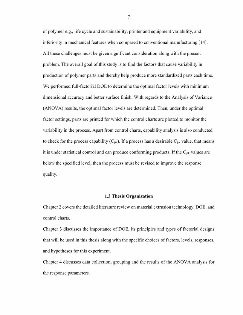
properties and cooperate with low energy fabrication technologies [1]. In 2016, the

revenues from material sales for AM passed the value of 900 million USD (Fig 1) of

which the largest fraction were into photopolymers (350 million USD) [8]. As such there

is need to understand the efficiency and properties of polymers used for AM.

Fig 1: Worldwide revenues from AM material sales between 2000 and 2016 adopted from [13]

In this thesis, reproducibility of polymers is assessed by manufacturing polymeric

parts using FFF technology. There are challenges involved with additive manufacturing

7

of polymer e.g., life cycle and sustainability, printer and equipment variability, and

inferiority in mechanical features when compared to conventional manufacturing [14].

All these challenges must be given significant consideration along with the present

problem. The overall goal of this study is to find the factors that cause variability in

production of polymer parts and thereby help produce more standardized parts each time.

We performed full-factorial DOE to determine the optimal factor levels with minimum

dimensional accuracy and better surface finish. With regards to the Analysis of Variance

(ANOVA) results, the optimal factor levels are determined. Then, under the optimal

factor settings, parts are printed for which the control charts are plotted to monitor the

variability in the process. Apart from control charts, capability analysis is also conducted

to check for the process capability (Cpk). If a process has a desirable Cpk value, that means

it is under statistical control and can produce conforming products. If the Cpk values are

below the specified level, then the process must be revised to improve the response

quality.

1.3 Thesis Organization

Chapter 2 covers the detailed literature review on material extrusion technology, DOE, and

control charts.

Chapter 3 discusses the importance of DOE, its principles and types of factorial designs

that will be used in this thesis along with the specific choices of factors, levels, responses,

and hypotheses for this experiment.

Chapter 4 discusses data collection, grouping and the results of the ANOVA analysis for

the response parameters.

8

Chapter 5 discusses conclusions for the entire thesis research, gives recommendations for

future work, and shares some details of planned future work on this project.

9

CHAPTER 2. LITERATURE REVIEW

This chapter includes four sections. Chapter 2.1 discusses studies that consider

dimensional accuracy and surface roughness as the response parameters and studies that

worked on improving these features. Chapter 2.2 focuses on DOE applications in AM.

Chapter 2.3 presents the studies about control charts. Lastly, Chapter 2.4 points out the

research gap and points to the potential contribution of the research.

2.1. Dimensional Accuracy and Surface finish in AM

Dimensional accuracy and resolution of finished parts made with extrusion AM

processes depend on the process (e.g., layer thickness, printing speed, raster angle) and

product design parameters, as well as the properties of the feedstock filament properties.

Aside from aesthetic considerations, these properties of the finished part can be critical

for applications where fit and form are important or when parts have very small feature

sizes [15]. Fused Deposition Modeling (FDM), Fused Filament Fabrication (FFF), 3D

dispensing, and 3D bio plotting are the examples of the material extrusion technology.

Gorski et al. [16] studied the effect of process parameters (e.g., layer thickness, part

orientation and filling strategy) on dimensional accuracy and reported that orientation

angle directly influences reproducibility of FFF technology. Tensile test specimens which

contain both straight and curved profiles are used to evaluate shape accuracy. Dul et al.

[17] built dumbbell and rectangular specimens along three different orientations i.e.,

horizontal, vertical and perpendicular. The direction of filament deposition changes with

the orientation. The importance of orientation effect was highlighted by the FDM process

10

while comparing 3D printed and compression molded parts. Moroni et al. [18]

determined that optimal part orientation is crucial for considering functional assembly in

case of a universal joint. Results show that the final recommended orientation angle is

different for individual part and assembly of universal joint. Ippolito et al. [5]

manufactured benchmark parts in FDM machine and showed that geometrical deviations

may reach up to +0.7 mm. Poor tessellation accuracy leads to inaccuracy in parts due to

errors in the data source. Hällgren et al. [19] compared the results of tessellation from six

different CAD systems, which showed that tessellation effects may be visible even when

dimensional requirements are fulfilled. Tessellation is the process of tiling a surface with

one or more geometric shapes such that there are no overlaps or gaps. They proposed a

method for 3D data exchange using traditional file format and geometric requirements.

AMF (Additive Manufacturing File Format) and 3MF (3D Manufacturing Format) are

still under development but can facilitate different materials and different densities in the

same part.

Giovanni et al. [18] proposed a methodology to estimate dimensional and geometric

deviation of features apart from its STL format by simulating the AM process

incorporating confounding errors from volumetric and material-related errors, such as

material flow and shrinkage. The cylindrical feature was selected in the study due to its

fundamental functionality in mechanical components. The case study considers the FDM

technology. The results show that it is reasonable to estimate the dimensional feature’s

deviation of the part from its STL file before fabrication given that the different types of

STL files have different effects on the response.

11

Lieneke et al. [2] developed a new method to analyze geometrical accuracies and

influencing factors based on the knowledge obtained by reviewing the dimensional

accuracies of FDM parts and observed the lack of geometric tolerances. This method

defines relevant geometries and influencing factors for the experimental tolerance

development. The derived tolerance values were also compared to values reached by

conventional manufacturing technologies. It was

concluded that the specifications of the key factors need to be varied to expand the

methodical procedure and determine the deviations for several geometrical shapes.

Unfortunately, FDM shows its main limits when the mechanical properties must go

hand in hand with surface finish [20]. Galantucci et al. [21] presented an in-depth

knowledge of the process that can improve the surface finish of FDM printed parts. The

author treated the FDM prototypes treated with a solution of 90% dimethyl ketone and

10% water to improve the surface finish and observed an increase in ductility and a

decrease in tensile strength. It was also observed that the angle of the filaments loses its

influence on the mechanical properties, probably due to an improved isotropy (uniformity

in all orientations) after the treatment.

Nourghassemi [22] studied the effect of build angle and layer thickness on the surface

finish of the parts to establish a relation between the factors and surface finish. An

equation relating them was developed and is shown below:

12

𝑅 =

⎩⎪⎨

⎪⎧(69.28 ~ 72.36)

𝑡

𝑐𝑜𝑠𝜃, 0° ≤ 𝜃 ≤ 70°

(90𝑅 ° − 70𝑅 ° + 𝜃(𝑅 ° − 𝑅 °)), if 70° < 𝜃 < 90°

117.6 X t, if θ = 90°𝑅 ( )°(1 + 𝑤) if 90° < 𝜃 < 180°

(1)

Where θ is the build angle and t is the layer thickness, Ra is the arithmetic-mean-surface

roughness in micron and w is a dimensionless adjustment parameter for supported facets

and chosen to be 0.2 for FDM system. One more interesting thing is that, when parts are

printed with the same specifications on a different printer, a difference was observed in

the values of surface finish.

Garg et al. [23] investigated the effect of part orientation on surface finish and

dimensional accuracy of FDM parts built at seven different part orientations (00, 150, 300,

450, 600, 750 & 900 about Y-axis) with and without post-building chemical vapor

treatment. From the results, it has been observed that a reasonable low surface finish is

obtained at 900 part build orientation for each primitive surface of the FDM part. To

obtain a minimum dimensional deviation of parts, surfaces of the FDM part should be

orientated either in parallel or in a perpendicular direction with respect to the axis of a

part. Post-built treatment with cold vapors of acetone yielded a dramatic improvement in

the surface finish due to a reduction in staircase effect present on surfaces. Surface

roughness values as low as 0.02 mm can be achieved. Chemical treatment of the

specimen causes a very minimal change in dimensional accuracy, and in many cases

reduction in dimensional deviation is achieved. Chemical treatment also leads to

rounding of the corners i.e., radius less than 1 mm is obtained. Thus, chemical treatment

13

with cold vapor could be used as an excellent alternative for FDM parts to improve

surface quality without much sacrifice in dimensional or geometry loss.

Sheydaeian et al. [24] manufactured Titanium structures for orthopedic applications

using the principle of Binder jet 3D printing multi-scale 3D printer by varying layer

thickness during the process. The specimens are cylindrical samples, designed with 5 mm

diameter and 8 mm height and are grouped in to four categories. The first two categories

were printed with a single layer thickness of 20 µm throughout and in the second two

categories, the layer thickness was varied from high to low and then to high

(150 μm/80 μm/150 μm) (Category A) and from low to high (80 μm/150 μm/80 μm)

(Category B) in each batch, respectively. The latter two were designed with a

symmetrical distribution of layer thickness with similar weight (0.5) to investigate the

effect of layer thickness arrangement on mechanical properties of the specimens. Height

and diameter of each sample were measured three times with digital caliper before and

after sintering. ANOVA analysis revealed that there is a significant difference in both

height and diameter shrinkage among the categories. The first two categories showed a

lot more height difference compared to the next two categories.

A summary of all relevant studies is presented below in Table 2 from which we can

conclude that the layer thickness, orientation angle, printing speed, fill angle, shell

thickness, raster angle and power level did have significant effect on the response

parameters. Main effects and interaction effects of printing speed and layer thickness

have significant effect on overall length and height which were published in ISERC

conference paper [63].

14

Table2: Summary of relevant studies

Author Material Technology Factors Responses Significant

factors

Galantucci et al. 2010

ABS FFF Chemical treatment

Surface finish -

Ranga et al. 2010

ABSP400 FDM

layer thickness, orientation,

raster angle & width

Dimensional accuracy

Thickness and raster

angle

Chang et al. 2011

ABS FDM

Layer thickness, fill

angle, orientation

Manufacturing time, surface

finish and tensile strength

Layer thickness, fill angle

Nourghasemmi et

al. 2011 PLA FDM

Build orientation and layer thickness

Relation between factors and

surface finish

Orientation angle, thick

ness

Singh 2014 ABS FDM Orientation Length, height Orientation

angle

Nidagundi et al. 2015

ABS-PA-747

FDM Layer thickness

fill angle

Dimensional accuracy, Surface

roughness

Layer thickness

Tateno et al. 2015

PLA FDM Thickness Cylindricity, Squareness

Thickness

Garg et al. 2016

ABS (P430) FDM Orientation Surface finish

and dimensional accuracy

Orientation

Fahad et al. 2017

Duraform polyamide (Nyl

on 12)

High-speed sintering (HSS)/Selective laser sintering

(SLS)

Layer thickness,

printing speed, power level

Flatness, Squareness

Layer thickness, printing speed

Sheydaeian et al. 2017

Titanium Binder jet Layer

thickness

Dimensional accuracy &

tensile strength tensile strength

Thickness

Vishwas et al. 2017

ABS FDM Shell thickness, layer thickness

Dimensional accuracy,

Time took

Layer and shell

thickness

Velineni et al. 2018

PLA FDM

Layer thickness,

printing speed, orientation angl

e

Dimensional features, surface

roughness

Different combinations of factors for different responses

15

Different parameters effect differently in the presence of other factors and at different

levels. Therefore, the combination of layer thickness, printing speed and orientation angle

which has not been studied is considered to determine the effect on dimensional accuracy

and surface finish.

2.2 Design of Experiments and applications

Before setting up a new manufacturing process to produce parts, it is necessary to

study the effect of process variables on the output. When a process involves multiple

factors, there is more chance for the output to be inconsistent as there is no fixed trend for

variability. It is necessary to consider the effect of both individual effects and interaction

effects and the latter is believed to have a significant influence on the response

parameters yet are often ignored. DOE is an efficient procedure to investigate the effect

of process parameters on the output so that the obtained results can be analyzed to yield

valid conclusions. It is used to determine the factors that causes the variation in response

and find the optimal conditions under which desirable response (minimum or maximum)

is achieved [25].

Several DOE studies focus on determining the optimal factor levels for the AM

process parameters in order to print the parts in desired quality. Albert [26] adopted 25

full factorial experiment with 5 factors being laser power, laser spot diameter, laser scan

speed, feature thickness and support structure. Melt pool stress and center feature stress

are the response parameters. There was a total of 64 runs including a complete set of

cases for each of two materials. Vishwas et al. [7] used Taguchi approach for design

16

optimization method as it provides a systematic and efficient procedure within a reduced

number of runs. As this approach involves a reduced number of experiments, cost and

time will be relatively less compared to a full-factorial design. With layer thickness,

orientation, and shell thickness as the three factors and with three levels each, Taguchi

orthogonal array with 9 runs (27 runs in case of full factorial) is used. ANOVA analysis

was used for Signal-to-Noise ratios to interpret the results. The results showed that the

best results were obtained with 0.3mm layer thickness, 300 orientation angle and 0.8 mm

shell thickness. Nidagundi et al. [8] adopted the same Taguchi approach for a 3-level 3

factor experiment. Three factors being layer thickness, orientation angle, and fill angle

with three levels each used the L9 orthogonal array. The advantages of this approach

include simplification of the experimental plan and feasibility of a study of the interaction

between various process parameters. The response parameters are surface roughness,

ultimate tensile strength, and dimensional features [5]. It is observed that higher ultimate

strength and optimal dimensional accuracy were observed at 0.1mm layer thickness, 0 °

orientation angle and 0° fill angle. Minimum surface roughness was observed at 0.3 mm

layer thickness, 150 orientation angle and 00 fill angle.

There are studies that considered the effect of layer thickness, part build orientation

angle, raster angle, raster to raster gap, and raster width on the dimensional accuracy of

FDM printed parts [27]. Raster angle is measured from x-axis on the bottom layer of the

part to the angle at which the layer is deposited. Both main effects and interaction effects

are considered to comment on the significance of factors. Process parameters were

optimized by using Taguchi’s L9 orthogonal array on the tensile testing specimen.

Significant process parameters were identified using ANOVA. The main effect plots for

17

signal-to-nose ratios for dimensional accuracy and manufacturing time are plotted. By

observing the experimental results, dimensional accuracy is maximum at 0.3 mm layer

thickness, 30° orientation angle, and 0.8 mm shell thickness. It is concluded that the

thinner layer thickness gives better bonding strength and gives good axial loading

capability. Upon varying layer thickness and orientation angle, the bonding strength

changes between the layers. Chang and Huang [28] considered layer thickness, fill angle,

orientation angle with three levels each to print specimens with ABS material using FDM

technology. They used the Taguchi method to select a specific set of runs instead of

selecting all 27. The response parameters were an ultimate tensile strength, surface finish

and manufacturing time. One of the limitations with this study is that authors did not

incorporate interaction effects between factors on each response since they implemented

the Taguchi method.

2.3 Control charts and capability studies

Control charts, a crucial tool in statistical quality control, can be classified as

control charts for variables and control charts for attributes [29]. The first category

contains control charts for individual measurements that are common in 3D printing.

However, such control charts are designed for identical products, which seldom

happen in 3D printing. The second category contains control charts for attributes that

have great potential to be applied to 3D printing. For example, the number of defects on a

3D-printed object is a critical problem. Under the assumption that the number of defects

on a unit of surface follows a Poisson distribution, control charts for nonconformities

(defects) can be constructed to minimize the number of defects [29]. They also check the

18

sample to sample variation to determine the variation is within the established stable

range.

X-R charts are ideal for smaller sample sizes and S charts are typically used for larger

sample sizes. The "chart" consists of a pair of charts: One to monitor the process standard

deviation and another to monitor the process mean. The Xand R chart plots the mean

value for the quality characteristic across all units in the sample Xi plus the range of the

quality characteristic in the sample as R=Xmax-Xmin, where Xmax shows the maximum

value of the quality characteristic while Xmin shows the minimum.

Process capability analysis entails comparing the performance of a process against its

specifications. It is a statistical measurement of a process’s ability to produce parts

within specified limits on a consistent basis. Cp (Process Capability), Cpk (Process

Capability Index), or Pp (Preliminary Process Capability) and Ppk (Preliminary Process

Capability Index) can be calculated to monitor how the processes are operating. The Cp

and Cpk calculations use sample deviation or deviation mean within rational subgroups.

Cp tells if your process is capable of making parts within specifications and Cpk shows if

your process is centered between the specification limits. They can be calculated using

the following formula [30]:

C =USL − LSL

6σ

C = MinUSL − μ

3σ,μ − LSL

3σ

Where USL and LSL are the upper and lower specification limits, μ is mean of the

process, σ is the standard deviation of the process.

19

Rupender Singh [6] plotted X and R charts for the feature groove width (10mm) of

parts produced by FDM, a highly capable process which helps us determine if a process

is stable and predictable. The X-bar chart shows how the mean or average changes over

time and the R chart shows how the range of the subgroup's changes over time.

Graphically, we assess process capability by plotting the process specification limits on

a histogram of the observations. If the histogram falls within the specification limits, then

the process is capable. It is observed that the Cpk value of 1.33 or greater is considered to

be the industry benchmarks. The response parameters being hardness, surface finish and

nominal dimensions had Cpk value greater than 1.33, so this process will produce

conforming products if it remains in statistical control. Also, the control chart of these

features had response values within the upper and lower control limits.

2.4 Research gap and contribution of the study

From the review of past potential studies, various studies considering different

factorial designs, factors, and responses are compared and it is observed that most of the

studies either considered one or two factors at a time and only very few studies

considered three factors at a time. We set up a full factorial design of experiment with

three factors layer thickness, printing speed and orientation angle and considered

interaction effects along with main effects. Our goal is to determine if the significant

factors still remain the same when both main effects and interaction effects are

considered. Once the significant factors are determined, a capability analysis is conducted

to test if the FFF process can produce PLA parts within specifications. Not only factors

but changing the 3D printer also affects the dimensional features. From literature review

on dimensional accuracy and surface finish studies, there is a need to examine the effect

20

of multiple factors on the response parameters. Different combination of factors has a

different effect on the output parameters of parts. This thesis is an effort made to

understand the effect of the three mentioned factors on dimensional accuracy and surface

finish. In this thesis, the full factorial design is used to avoid data loss about output

variability. As the specimens are smaller in size, the cost factor didn’t play a major role in

our study. Since the FFF process is one of the most important and widely used

technologies, it has been closely studied regarding the relationship between mechanical

properties, dimensional features, surface finish and process parameters [31].

21

CHAPTER 3. METHODOLOGY

In a production environment, it is important to manage the variation in the process in

order to maintain a specified level of quality. There are many reasons of variation due to

controllable factors and uncontrollable factors. Controllable factors are the ones which

we may set their levels during the process; however, the levels of uncontrollable factors

cannot be set. The general view of a process showing the cause of variations is presented

in Fig 2.

Fig 2: General model of a process [32]

Different applications of additive manufacturing may require different levels of input

variables/process parameters. It is necessary to study the effect of various levels of

factors on the output parameters to improve productivity and quality. All engineering

processes in a manufacturing organization are subject to variation, sources of which may

be combinations of materials, equipment, method or environmental conditions [33].

Because of the limited resources available, experimentation is the best choice to [34]

reduce time to design/develop new products & processes

improve the performance of existing processes

22

improve reliability and performance of products

achieve product & process robustness

perform an evaluation of materials, design alternatives, setting component &

system tolerances, etc.

It is beneficial to work beforehand in selecting the suitable levels of controllable

factors rather than working for a solution after sensing the problem. To finalize optimal

conditions for a process, the factors are varied within a reasonable range and the response

parameters are measured and analyzed to conclude the effect of different levels of factors.

Response parameters are the output of the process which shows the quality level of

interest. When two or more variables are involved in an experimental study, there is more

to consider than simply the main effect. The effect of one independent variable may

depend on the level of the other independent variables [35]. Often interaction effects are

ignored to avoid the complexity which shouldn’t be the practice.

Main effect - the effect of a single independent variable on the response ignoring

all other process variables.

Interaction effect – When the effect of a factor on the product or process is

altered due to the presence of one or more other factors, that relationship is called

an interaction effect.

DOE plays an important role in Design for Reliability (DFR) programs, allowing the

simultaneous investigation of the effects of various factors and thereby

facilitating design optimization.

23

3.1 Design of Experiments (DOE)

DOE is one such methodology that can involve multiple factors in a process. It is

defined as a series of tests in which purposeful changes are made to the input variables of

a system or process to observe and identify the reasons for changes in responses [36]. The

response values are analyzed by ANOVA using statistical packages like Minitab, JMP,

Stat graphics, R, SPC XL, etc. DOE can also be understood as a crucial technique that is

used to find if the key inputs are related to key outputs based on statistical analysis [37].

DOE can accommodate experiments where multiple factors can be varied at once. DOE

is more beneficial and convenient because it involves fewer runs, less time, and less

material usage, it includes the effect of interactions, estimated effects of variables are

more precise, and it maximizes the amount of information gained while minimizing the

amount of data to be collected [38].

3.2 Important Principles of DOE

3.2.1 Randomization

An essential component of every experiment that needs to be validated. Generally, it is

extremely difficult for researchers to eliminate unknown potential bias using only their

expert judgment or literature review, so a deliberate process which randomizes the

experiment to eliminate these biases from the conclusions is required. In a randomized

experimental design, objects or individuals are randomly assigned to an experimental

group [39,40]. Using randomization is the most reliable method of creating homogeneous

treatment groups, without involving any potential biases or judgments. From various

types of randomizations available, two types of it are discussed below:

24

a) Completely randomized design

In a completely randomized design, objects or subjects are assigned to groups

completely at random. One standard method for assigning subjects to treatment groups is

to label each subject, then use a table of random numbers to select from the labeled

subjects. This may also be accomplished using a computer [41]. In MINITAB, the

"SAMPLE" command will select a random sample of a specified size from a list of

objects or numbers.

b) Randomized block design

If an experimenter is aware of specific differences among groups of subjects or objects

within an experimental group, the experimenter may prefer a randomized block design to

a completely randomized design. In a block design, experimental subjects are first

divided into homogeneous blocks before they are randomly assigned to a treatment group

[42]. For easy understanding, let us assume that an experimenter had reason to believe

that a factor in an experiment might have a significant effect on the response, he might

choose to first divide the experimental subjects into groups based on the levels of factors

considered. Then, the segregated groups would be assigned to treatment groups using a

completely randomized design [43]. In a block design, both control

and randomization are considered. In our present study, we used the completely

randomized experiments using MINITAB to randomize the experiment runs as there was

no potential grouping of factors was seen.

3.2.2 Replication

To understand the concept of replication, let’s revise the definition of the standard

error of the mean. It is the square root of the estimate of the variance of the sample mean.

25

The width of the confidence interval is determined by this statistic. The estimates of the

mean become less variable as the sample size increases. Replication is the basic issue

behind every method used to estimate or control the uncertainty in our results [44]. But it

is important to note the difference between replicated runs and repeated runs, although

the multiple response readings are taken at the same factor levels for both. However,

repeated runs are response observations taken at the same time or in succession whereas

replicated runs are response observations recorded in a random order. Therefore,

replicated runs include more variation than repeated runs [45].

3.3 Factorial Designs

A factorial design is one of the important principles examining several factors

simultaneously. The factorial experiments, where all combinations of the levels of the

factors are run, are usually referred to as full factorial experiments.

3.3.1 Two-level factorial design

Full factorial two-level experiments are also referred to as 2K designs

where K denotes the number of factors in the experiment. A full factorial two-level

design with K factors requires 2K runs for a single replicate [46]. For example, a two-

level experiment with three factors will require 23 = 8 runs. The first level, i.e. lower

level, of the factors are usually represented as -1, while the second level, i.e. higher level,

is presented as +1.

3.3.2 Three-level factorial design

Similar to two-level, three-level factorial designs are referred to as 3K designs, where

K shows the number of factors. For instance, a three-level experiment with three-factor

26

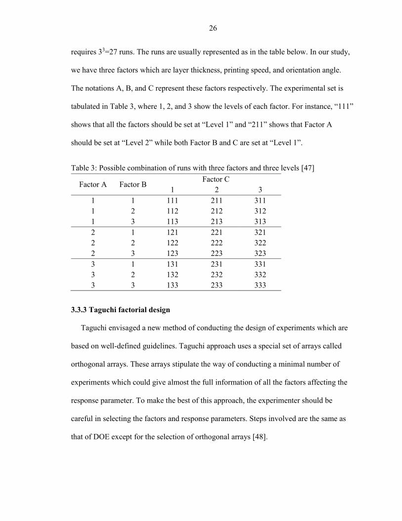
requires 33=27 runs. The runs are usually represented as in the table below. In our study,

we have three factors which are layer thickness, printing speed, and orientation angle.

The notations A, B, and C represent these factors respectively. The experimental set is

tabulated in Table 3, where 1, 2, and 3 show the levels of each factor. For instance, “111”

shows that all the factors should be set at “Level 1” and “211” shows that Factor A

should be set at “Level 2” while both Factor B and C are set at “Level 1”.

Table 3: Possible combination of runs with three factors and three levels [47]

3.3.3 Taguchi factorial design

Taguchi envisaged a new method of conducting the design of experiments which are

based on well-defined guidelines. Taguchi approach uses a special set of arrays called

orthogonal arrays. These arrays stipulate the way of conducting a minimal number of

experiments which could give almost the full information of all the factors affecting the

response parameter. To make the best of this approach, the experimenter should be

careful in selecting the factors and response parameters. Steps involved are the same as

that of DOE except for the selection of orthogonal arrays [48].

Factor A Factor B Factor C

1 2 3 1 1 111 211 311 1 2 112 212 312 1 3 113 213 313 2 1 121 221 321 2 2 122 222 322 2 3 123 223 323 3 1 131 231 331 3 2 132 232 332 3 3 133 233 333

27

To determine the effect each variable has on the output, the signal-to-noise ratio needs

to be calculated for each experiment conducted. Taguchi's method for experimental

design is straightforward and easy to apply to many engineering situations, making it a

powerful yet simple tool. It can be used to quickly narrow down the scope of a research

project or to identify problems in a manufacturing process from data already in existence.

Also, the Taguchi method allows for the analysis of many different parameters without a

prohibitively high amount of experimentation [49]. One of the disadvantages is that the

results obtained do not exactly indicate which parameter has a highest significant effect

on output. Also, since orthogonal arrays do not test all variable combinations, this method

should not be used if there’s no room for risk of losing data. Another limitation is that the

Taguchi methods are offline, and therefore inappropriate for a dynamically changing

process such as a simulation study [49].

Some uncontrollable noise factors cause the quality characteristics to deviate from the

target values. The factors can be classified into three categories: 1) external factors, 2)

manufacturing imperfections, and 3) product deterioration. The unstable environment

conditions, such as power supply, temperature, humidity and vibrations of nearby

machinery, are the external factors. The Orthogonal Array (OA) is used as part of the

Taguchi Method to design the experiments. OA is a systematic, statistical way of testing

pair-wise interactions. It provides representative (uniformly distributed) coverage of all

variable pair combinations.

28

a) Signal-to-Noise Ratio and Analysis of Variance

The sample signal to noise ratio is defined as the ratio of the mean to the standard

deviation. It shows the variability as defined by the standard deviation relative to the

mean. This definition of the signal to noise ratio should typically only be used for data

measured on a ratio scale. That is, the data should be continuous and have a meaningful

zero. Typically, there are three S/N ratios: the lower-the-better (people desire the quality

characteristic value to be small, such as surface roughness), the higher-the-better (such as

mechanical strength), and the nominal-the-better (such as the dimension). The unit of S/N

is dB, the lower-the-better S/N calculation [50] is presented in Equation (1).

S

N= −10 x log (

1

nY )

(2)

where n is the number of measurements and Yi is the observed performance

characteristic value. After the S/N value is calculated, a statistical method called analysis

of variance (ANOVA) will be performed. ANOVA is used to evaluate the influence of

the control factors on the experimental results and to determine which control factors are

statistically significant [51].

3.4. Development of the Experiment

Having understood the importance of main effects and interaction effects, we can

determine significant factors by running a full complement of all factor combinations,

i.e., a full factorial design. We have adopted a full factorial design in our study to avoid

missing any information about output variability, main effects, and interaction effects.

Research is conducted in order to determine the factors that are responsible for

29

dimensional accuracy and surface finish for material extrusion technology when

polymers are used.

Even though studies exist tackling the effect of printing speed on surface finish [17,

52, 53,54], there is a need to investigate its effect on dimensional accuracy. Moreover,

the interaction effect of build orientation between factors layer thickness and printing

speed has not been investigated for FFF technology and polymers. In order to address

these gaps in the literature, we investigate the main and interaction effects of printing

speed, layer thickness, and build orientation for FFF technology and PLA material. The

levels of these three factors are presented in Table 4,

Table 4: Three factors with three different levels each

With regards to the findings of the literature review, the goal of this study is to

investigate the effect of layer thickness, printing speed, and orientation angle on

dimensional accuracy and surface roughness. Therefore, our hypothesis is that the part’s

dimensional accuracy for overall length, height, width, middle height, and surface

roughness might be affected by all the three factors. We consider three factors: layer

thickness, printing speed and orientation angle with three levels constituting 27 different

experiments. All the experiments were replicated thrice, summing to a total of 81 runs.

Factor Factor labels Level 1 Level 2 Level 3

Layer thickness(mm) A 0.1 0.2 0.3

Printing Speed(mm/s)

B 60 80 100

Orientation angle C 00 450 900

30

The full factorial method was used to investigate the main effects of factors, and

interaction effects between the factors.

We ran all 81 experiments randomly without following any order so that the machine

can be set to different process parameters rather than replicating the same parts thrice in a

row. All experiments are run under the same conditions; all other factors except layer

thickness, printing speed, and orientation angle were kept constant for all experiments.

We used PLA polymer to build the parts on the FFF machine. The FFF 3D printer that we

used is Monoprice Maker Select V2 (Fig 3) with build volume 8"x8"x7", 100-micron

resolution, 1.75mm filament diameter, 100mm/sec print speed and max temperature of

2600C. The price of PLA coil 1.75mm thickness, 1kg spool was 15$. As PLA material is

relatively cheap compared to other polymers, full factorial DOE is considered instead of

reduced factorial methods. The price of the 3D printer, Monoprice maker select V2 was

200$.

Fig 3: Monoprice maker select V2 3D printer

Monoprice maker in Fig 3 is the 3D printer used to print PLA parts. A memory card is

used to load the STL file to the printer. The building part in Fig 5(a) is a dog bone shaped

31

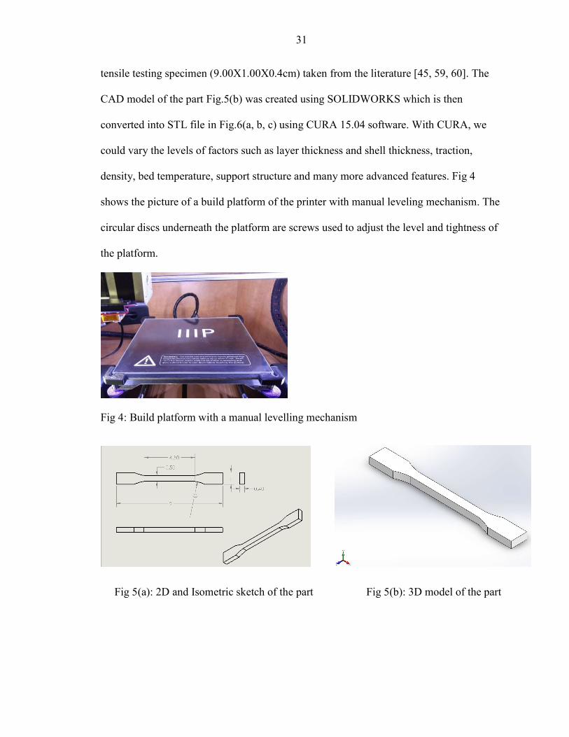
tensile testing specimen (9.00X1.00X0.4cm) taken from the literature [45, 59, 60]. The

CAD model of the part Fig.5(b) was created using SOLIDWORKS which is then

converted into STL file in Fig.6(a, b, c) using CURA 15.04 software. With CURA, we

could vary the levels of factors such as layer thickness and shell thickness, traction,

density, bed temperature, support structure and many more advanced features. Fig 4

shows the picture of a build platform of the printer with manual leveling mechanism. The

circular discs underneath the platform are screws used to adjust the level and tightness of

the platform.

Fig 4: Build platform with a manual levelling mechanism

Fig 5(a): 2D and Isometric sketch of the part Fig 5(b): 3D model of the part

32

Fig 6(a): Part Orientation in CURA15.04 software with 00

Fig 6(c): Part Orientation in CURA15.04 software with 900

The printing duration for building each part varies with the levels of factors. Though

the factors layer thickness and printing speed are kept constant, the building time of each

part varies when the build orientation is changed. The depositing direction, i.e build

orientation, changes to horizontal, inclined or vertical depending on the angle. The setup

of Factor A in Level 3, Factor B in Level 3 and Factor C in Level 2 took the least time of

5 min per part. The set up with Factor A in Level 1, Factor B in Level 1 and Factor C in

Level 1 took the longest printing time of 18 min per part. Table 5 shows the time taken to

Fig 6(b): Part Orientation in CURA15.04 software with 450

33

print each part at different levels of factors. In Table 5, 1, 2, 3 refer to the levels of each

factor.

Table 5: Manufacturing time required for each run

The methodology, experimental set up, and equipment are clearly discussed in this

chapter. The results and the effects of input on output parameters will be explained in

chapter 4

Factor Levels

A B C Time (Min)

1

1 1 18 2 17 3 18

2 1 16 2 15 3 16

3 1 14 2 13 3 14

2

1 1 10 2 10 3 10

2 1 9 2 8 3 9

3 1 8 2 7 3 8

3

1 1 7 2 7 3 7

2 1 6 2 6 3 6

3 1 6 2 5 3 6

34

CHAPTER 4. RESULTS & DISCUSSIONS

All the parts with different levels of factors are printed according to the DOE plan and

procedures discussed in Chapter 3. A full factorial design of experiment is performed for

each level of layer thickness, printing speed, and orientation angle. Layer thickness is the

thickness of the material being deposited on the build platform from the nozzle of a 3D

printer. Printing speed is the speed at which the nozzle moves with respect to the

stationary bar of the 3D printer. Orientation angle is the angle which can be set through

CURA software so that the part will be printed in that angle on the build platform, i.e. the

angle at which the layers are deposited will change for different orientations.

After experiments, the end products are measured. Overall length is the horizontal

length of the part from extreme right to extreme left point of the part. Height is the

vertical distance from top most point to lowest point of the part when its placed as the top

part as shown in the Fig 5(a). Width is the thickness of the part and middle height is the

vertical distance of the part in the middle section. Instead of considering the actual

measured dimensional values for analysis, the values are subtracted from the nominal

dimensions of the part to provide a direction and aim to the analysis. The aim is to

minimize the deviation of the response values from target values. All four dimensions are

measured at the same location on each part using digital Vernier calipers with an

accuracy of 0.001mm. Table 6 shows the actual measured values whereas Table 7 shows

the absolute value of difference of measured response parameters from nominal values.

The percentage change in each dimension i, i=length, width, height, is calculated based

on Eq. (2), where 𝑋 shows the measured value for dimension i, and 𝑋 shows the

respective CAD dimension of the part. The term %∆𝑋 , stands for the percentage change

35

according to the CAD value for each dimension i. It should be noted that the higher

percentage deviations refer to lower dimensional accuracy. R1, R2, and R3 presents to

1st, 2nd, and 3rd replicas of the experiment.

%∆𝑋 =|𝑋 − 𝑋 |

𝑋× 100

(3)

A, B, C columns in Table 6 and Table 7 are used to represent the factors and

corresponding levels. Since the full-factorial design was repeated thrice, R1, R2, and R3

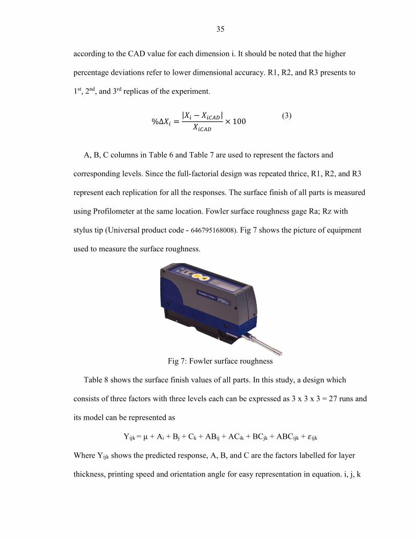
represent each replication for all the responses. The surface finish of all parts is measured

using Profilometer at the same location. Fowler surface roughness gage Ra; Rz with

stylus tip (Universal product code - 646795168008). Fig 7 shows the picture of equipment

used to measure the surface roughness.

Fig 7: Fowler surface roughness

Table 8 shows the surface finish values of all parts. In this study, a design which

consists of three factors with three levels each can be expressed as 3 x 3 x 3 = 27 runs and

its model can be represented as

Yijk = µ + Ai + Bj + Ck + ABij + ACik + BCjk + ABCijk + 𝜀ijk

Where Yijk shows the predicted response, A, B, and C are the factors labelled for layer

thickness, printing speed and orientation angle for easy representation in equation. i, j, k

36

are the levels of factors respectively and 𝜀 shows the error term. These terms are used for

all regression equations in this study. In this case, main effects have 2 degrees of

freedom, two-factor interactions have 4 degrees of freedom and similarly, k-factor

interactions have 2K degrees of freedom. This model contains a total of 26 degrees of

freedom.

37

Table 6: Measured values of dimensional response parameters in mm.

Overall Length (mm) Height (mm) Width (mm) Middle height (mm) Run LT PS OA R1 R2 R3 R1 R2 R3 R1 R2 R3 R1 R2 R3

1

0.1

60 0 8.960 8.983 8.970 1.006 1.010 1.004 0.382 0.389 0.389 0.512 0.516 0.514 2 60 45 8.950 8.950 8.959 1.005 1.000 1.003 0.378 0.385 0.370 0.507 0.509 0.506 3 60 90 8.981 8.967 8.960 1.000 1.000 1.003 0.374 0.391 0.354 0.505 0.505 0.503 4 80 0 8.980 8.971 8.980 1.000 1.000 0.994 0.372 0.362 0.360 0.508 0.511 0.515 5 80 45 8.976 8.985 8.974 1.002 1.003 1.004 0.372 0.387 0.335 0.510 0.503 0.505 6 80 90 8.970 8.960 8.975 1.010 1.000 1.005 0.388 0.392 0.389 0.512 0.511 0.512 7 100 0 8.970 8.968 8.967 0.993 0.996 0.994 0.399 0.395 0.395 0.507 0.503 0.503 8 100 45 9.000 8.976 8.997 0.990 1.000 0.989 0.394 0.373 0.404 0.496 0.501 0.499 9 100 90 8.986 8.984 8.950 0.990 0.998 0.998 0.391 0.368 0.368 0.504 0.507 0.506 10

0.2

60 0 8.980 8.966 8.970 0.995 0.995 1.000 0.398 0.396 0.400 0.509 0.504 0.509 11 60 45 8.990 8.982 8.976 1.000 0.993 0.992 0.408 0.404 0.408 0.497 0.499 0.494 12 60 90 8.970 8.973 8.966 0.997 0.992 0.993 0.409 0.406 0.408 0.499 0.499 0.497 13 80 0 8.960 8.980 8.983 0.992 0.980 0.984 0.361 0.385 0.322 0.488 0.499 0.496

14 80 45 8.983 8.925 8.980 0.993 0.990 0.994 0.397 0.385 0.397 0.495 0.484 0.493 15 80 90 8.979 8.971 8.980 0.996 0.992 0.993 0.400 0.378 0.371 0.487 0.494 0.492 16 100 0 8.958 8.959 8.962 0.989 0.973 0.987 0.404 0.406 0.409 0.485 0.485 0.490 17 100 45 8.954 8.954 8.946 0.976 0.975 0.984 0.410 0.370 0.367 0.476 0.479 0.480 18 100 90 8.952 8.973 8.969 0.995 0.979 0.984 0.374 0.377 0.384 0.488 0.486 0.483 19

0.3

60 0 8.960 8.960 8.938 0.980 0.980 0.989 0.377 0.381 0.375 0.494 0.486 0.494 20 60 45 8.988 8.997 9.000 0.979 0.984 0.992 0.400 0.410 0.411 0.483 0.494 0.498 21 60 90 8.965 8.960 8.960 0.976 0.978 0.981 0.392 0.390 0.392 0.483 0.486 0.486 22 80 0 8.966 8.967 8.970 0.988 0.984 0.988 0.389 0.389 0.388 0.498 0.496 0.500 23 80 45 8.961 8.937 8.992 0.977 0.981 0.979 0.369 0.388 0.385 0.478 0.481 0.483 24 80 90 8.969 8.971 8.965 0.986 0.984 0.988 0.339 0.340 0.386 0.490 0.479 0.483 25 100 0 8.977 8.980 8.978 0.980 0.990 0.998 0.381 0.336 0.334 0.517 0.506 0.507 26 100 45 8.981 8.970 8.994 0.993 0.990 0.976 0.388 0.352 0.391 0.484 0.485 0.491 27 100 90 8.960 8.942 8.940 0.976 0.992 1.000 0.368 0.363 0.360 0.560 0.522 0.520

38

Table 7: Absolute deviation values of dimensional features in mm Overall Length (mm) Height (mm) Width (mm) Middle height (mm)

Run LT PS OA R1 R2 R3 R1 R2 R3 R1 R2 R3 R1 R2 R3

1

0.1

60 0° 0.040 0.017 0.030 0.006 0.010 0.004 0.018 0.011 0.011 0.012 0.016 0.014

2 60 45° 0.050 0.050 0.041 0.005 0.000 0.003 0.022 0.015 0.030 0.007 0.009 0.006

3 60 90° 0.019 0.033 0.040 0.000 0.000 0.003 0.026 0.009 0.046 0.005 0.005 0.003

4 80 0° 0.020 0.029 0.020 0.000 0.000 0.006 0.028 0.038 0.040 0.008 0.011 0.015

5 80 45° 0.024 0.015 0.026 0.002 0.003 0.004 0.028 0.013 0.065 0.010 0.003 0.005

6 80 90° 0.030 0.040 0.025 0.010 0.000 0.005 0.012 0.008 0.011 0.012 0.011 0.012

7 100 0° 0.030 0.032 0.033 0.007 0.004 0.006 0.001 0.005 0.005 0.007 0.003 0.003

8 100 45° 0.000 0.024 0.003 0.010 0.000 0.011 0.006 0.027 0.004 0.004 0.001 0.001

9 100 90° 0.014 0.016 0.050 0.010 0.002 0.002 0.009 0.032 0.032 0.004 0.007 0.006

10

0.2

60 0° 0.020 0.034 0.030 0.005 0.005 0.000 0.002 0.004 0.000 0.009 0.004 0.009

11 60 45° 0.010 0.018 0.024 0.000 0.007 0.008 0.008 0.004 0.008 0.003 0.001 0.006

12 60 90° 0.030 0.027 0.034 0.003 0.008 0.007 0.009 0.006 0.008 0.001 0.001 0.003

13 80 0° 0.040 0.020 0.017 0.008 0.020 0.016 0.039 0.015 0.078 0.012 0.001 0.004

14 80 45° 0.017 0.075 0.020 0.007 0.010 0.006 0.003 0.015 0.003 0.005 0.016 0.007

15 80 90° 0.021 0.029 0.020 0.004 0.008 0.007 0.000 0.022 0.029 0.013 0.006 0.008

16 100 0° 0.042 0.041 0.038 0.011 0.027 0.013 0.004 0.006 0.009 0.015 0.015 0.010

17 100 45° 0.046 0.046 0.054 0.024 0.025 0.016 0.010 0.030 0.033 0.024 0.021 0.020

18 100 90° 0.048 0.027 0.031 0.005 0.021 0.016 0.026 0.023 0.016 0.012 0.014 0.017

19

0.3

60 0° 0.040 0.040 0.062 0.020 0.020 0.011 0.023 0.019 0.025 0.006 0.014 0.006

20 60 45° 0.012 0.003 0.000 0.021 0.016 0.008 0.000 0.010 0.011 0.017 0.006 0.002

21 60 90° 0.035 0.040 0.040 0.024 0.022 0.019 0.008 0.010 0.008 0.017 0.014 0.014

22 80 0° 0.034 0.033 0.030 0.012 0.016 0.012 0.011 0.011 0.012 0.002 0.004 0.000

23 80 45° 0.039 0.063 0.008 0.023 0.019 0.021 0.031 0.012 0.015 0.022 0.019 0.017

24 80 90° 0.031 0.029 0.035 0.014 0.016 0.012 0.061 0.060 0.014 0.010 0.021 0.017

25 100 0° 0.023 0.020 0.022 0.020 0.010 0.002 0.019 0.064 0.066 0.017 0.006 0.007

26 100 45° 0.019 0.030 0.006 0.007 0.010 0.024 0.012 0.048 0.009 0.016 0.015 0.009

27 100 90° 0.040 0.058 0.060 0.024 0.008 0.000 0.032 0.037 0.040 0.060 0.022 0.020

39

Table 8: Measured values of surface roughness

‘-‘Device gave no reading at those level of factors

Table 8 lists the values of surface finish of eighty-one parts measured using

profilometer at same location. Ra is the arithmetic average of the absolute values of the

profile height deviations from the mean line, recorded within the evaluation length. Table

R1 R2 R3

Run LT PS OA Ra Ra Ra

1

0.1

60 0 2.90 4.10 7.90

2 60 45 11.21 1.41 1.76

3 60 90 7.14 5.92 7.02

4 80 0 6.12 12.01 7.22

5 80 45 12.08 15.21 9.11

6 80 90 1.58 3.97 5.13

7 100 0 13.35 16.78 15.09

8 100 45 1.56 3.12 1.76

9 100 90 9.36 10.00 10.30

10

0.2

60 0 9.37 8.07 11.89

11 60 45 3.71 21.53 1.46

12 60 90 5.13 8.23 5.10

13 80 0 15.18 17.41 5.56

14 80 45 19.78 2.63 13.12

15 80 90 21.22 14.25 21.22

16 100 0 7.00 12.11 24.17

17 100 45 34.27 39.01 45.26

18 100 90 24.76 19.81 21.08

19

0.3

60 0 36.12 7.41 15.11

20 60 45 3.01 1.18 2.09

21 60 90 21.52 8.22 10.55

22 80 0 45.28 21.22 15.55

23 80 45 - 12.58 27.61

24 80 90 37.81 49.44 -

25 100 0 - - 51.16

26 100 45 56.01 61.01 39.03

27 100 90 - 40.36 -

40

8 has some cells with ‘-’, which means the profilometer couldn’t give a reading at those

factor levels because of too large values. Simply put, Ra is the average of a set of

individual measurements of a surface’s peaks and valleys [56].

The Figures 8 (a) and 8 (b) show the resolution obtained at different factor levels.

Clearly, the Fig 8(a) is much finer when compared to 8(b).

Full factorial design of experiment is beneficial when considering multiple factors and

interaction effects between them. To examine the statistical significance of factors on

each response, we performed analysis of variance (ANOVA) method using Minitab 18

statistical software. Our hypothesis in this study is that the layer thickness, printing speed,

orientation angle and their interactions might have a significant effect on the deviation

Fig 8(a): Specimen with 0.1mm layer thickness, 60mm/s printing speed & 00

Fig 8(b): Specimen with 0.3mm layer thickness,100mm/s printing speed & 00

41

from nominal dimensions. A brief explanation of ANOVA interpretation is discussed

followed by the ANOVA results for deviation of all the responses.

4.1 Interpretation of ANOVA

Significant factors are those which cause a change on the output not due to chance.

Statistical evidence is used to comment on significance level of factors. ANOVA analysis

is used to determine the p-values which are used to assess the null hypothesis by

comparing them with the significance level. A significance level indicates the probability

of rejecting the null hypothesis given that it is true [57]. In our current example, we have:

Null Hypothesis (H0) – Response parameters are not affected by the input variables.

Alternative Hypothesis (H1) – Response parameters are affected by the input variables.

Small p-values (<=0.05) are counted as evidence against H0 and in favor of H1 in 95%

confidence. However, a p-value may not be interpreted as a "probability that H0 is true," a

quantity that is simply without a rational definition. So, even if we fail to reject the null

hypothesis, it does not mean the null hypothesis is true [58]. That's because

a hypothesis test does not determine which hypothesis is true, or even which is most

likely, it only assesses whether available evidence exists to reject the null hypothesis.

The following sections discuss about the results from the 81 experiments in Table 7

and Table 8. The basic summary statistics were calculated, an Analysis of Variance

(ANOVA) was performed, and model validation is done for each of the five responses. A

multivariate analysis of variance (MANOVA), is an analysis of variance except that there

are more responses involved. This is used in studies where more than one dependent

variables are affected by one or more factors. Various methods related to analysis of

variance like hypothesis testing, partitioning of sum of squares, additive models and

42

experimental techniques have been around the since the beginning of the 19th century.

ANOVA tests the differences between three or more groups means and it can assess only

one dependent variable at a time. ANOVA analysis is adopted in this study to test the

effects of dependent variables at a time and then study the effects of multiple factors from

interaction effects. ANOVA analysis for each response parameter is conducted separately

and is discussed simultaneously with main effect and interaction plots.

4.2. Optimal factor determination for overall length

The first step in the ANOVA process is to identify the potentially significant factors

and interactions. Factors/combinations affecting overall length will be discussed in this

section as each response parameter is analyzed separately. Before proceeding with the

ANOVA analysis, data must be checked for normality, because like other parametric

tests, ANOVA assumes that the data fits the normal distribution. If the measurement

variable (response parameter) is not normally distributed, there may be an increase in the

chance of a false positive result if analyzed with an ANOVA or another test that assumes

normality. If data is not normally distributed, many practitioners suggest that a non-

parametric version of the test which does not assume normality should be conducted.

Fig 9: Normality test for overall length

0.0750.0500.0250.000

99.9

99

9590

80706050403020

105

1

0.1

Mean 0.03040StDev 0.01486N 81AD 0.441P-Value 0.284

Overall length

Perc

ent

Probability Plot of Overall lengthNormal

43

Anderson-Darling test is used to test the normality of the data. In this test, null

hypothesis is H0: Data follows normal distribution and alternative hypothesis is H1: Data

does not follow normal distribution. In Fig 9, the p-value for Anderson-Darling test is

0.284. Thus, the decision is not to reject the null hypothesis in 90% confidence level. We

cannot conclude that the data is not normally distributed.

Our hypothesis is that all the factors and their interactions do not have significant

effects on the deviation in overall length. The ANOVA results are presented in Table 9.

Table 9: ANOVA results for deviation in overall length

According to the ANOVA results in Table 9, we observe that the interaction effect of

LT X PS, layer thickness and printing speed (p-value = 0.008), interaction effect of LT X

OA, layer thickness and orientation angle (p-value = 0.031) and interaction effect of all

three factors LT X PS X OA, (p-value = 0.001) have significant effects on the overall

length. The rest of the factors do not have significant effects on the response based on the

statistical evidence.

The Pareto chart is used to determine the magnitude and the importance of the effects.

On the Pareto chart, bars that cross the reference line are statistically significant [62].

With regards to the Pareto chart in Fig 10, the bars that represent factors LT X PS, LT X

Source DF SS MS F-Value P-Value LT 2 0.000003 0.000002 0.98 0.383 PS 2 0.000001 0.000000 0.27 0.767 OA 2 0.000008 0.000004 2.2 0.121 LT X PS 4 0.000026 0.000007 3.87 0.008 LT X OA 4 0.000020 0.000005 2.88 0.031 PS x OA 4 0.000012 0.000003 1.75 0.153 LTX PS X OA

8 0.000056 0.000007

4.09 0.001

Error 54 0.000092 0.000002 Total 80 0.000218

44

OA and LT X PS X OA cross the reference line that is 2.005. These factors are

statistically significant at the 0.05 level with the current model terms.

Fig 10: Pareto chart of standardized effects for overall length

4.2.1 Accuracy of the model

A very important part of an analysis is to test model validity, as an invalid model

produces invalid conclusions. Model adequacy is tested by examining the validity of

three assumptions for the residuals using a 4-in-1 residual plot: normality, equal

variances, and data independence [59]. A residual plot is a graph that is used to examine

the goodness of fit in regression and ANOVA. First, the normality of the residuals was

tested using a normal probability plot (please see Fig 11). This plot shows no outliers,

significant gaps or clear tails. Similarly, the histogram at the bottom left of Fig 11 clearly

displays a bell-shaped distribution indicating that the normality assumption of residuals is

satisfied.

Term

B

A

BC

C

AC

AB

ABC

43210

A AB BC C

Factor Name

Standardized Effect

2.005

Pareto Chart of the Standardized Effects(response is OL, α = 0.05)

45

Fig 11: Residual plots of overall length

The versus-fits plot in Fig 11 indicates the validity of the constant variance

assumption. In this case, the assumption is satisfied because the residual data had a nice

random spread, except for a couple of outliers right to the center but they don’t seem to

follow a specific pattern, so the independence assumption cannot be rejected. The versus

order plot (bottom right of Fig 11, “Versus Order”) is used to validate the independence

assumption. This plot is appropriate if you know the order in which the data is collected.

There is nothing extremely different about the plot except few points shooting long from

the center. In order to check the equal variance assumption, we plot variation in residuals

at different levels of treatment in Fig 12. The distribution of residual is very similar at all

three levels, so we can assume equality of variance between the levels. After all the

assumptions for the residuals are met, we identify the optimal factor settings in Section

4.2.2.

0.040.020.00-0.02-0.04

99.999

90

50

10

10.1

Residual

Perc

ent

0.0480.0360.0240.0120.000

0.04

0.02

0.00

-0.02

Fitted Value

Resi

dual

0.040.030.020.010.00-0.01-0.02-0.03

24

18

12

6

0

Residual

Freq

uenc

y

80706050403020101

0.04

0.02

0.00

-0.02

Observation OrderRe

sidu

al

Normal Probability Plot Versus Fits

Histogram Versus Order

Residual Plots for overall length

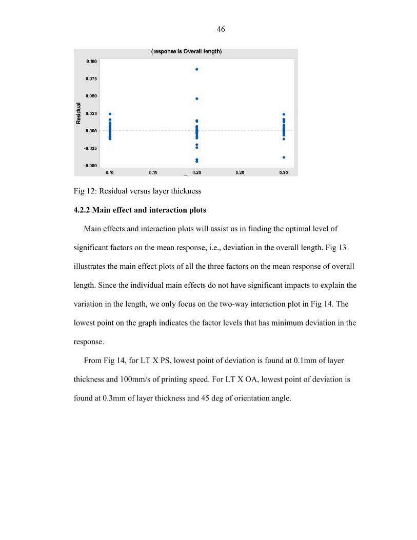
46

Fig 12: Residual versus layer thickness

4.2.2 Main effect and interaction plots

Main effects and interaction plots will assist us in finding the optimal level of

significant factors on the mean response, i.e., deviation in the overall length. Fig 13

illustrates the main effect plots of all the three factors on the mean response of overall

length. Since the individual main effects do not have significant impacts to explain the

variation in the length, we only focus on the two-way interaction plot in Fig 14. The

lowest point on the graph indicates the factor levels that has minimum deviation in the

response.

From Fig 14, for LT X PS, lowest point of deviation is found at 0.1mm of layer

thickness and 100mm/s of printing speed. For LT X OA, lowest point of deviation is

found at 0.3mm of layer thickness and 45 deg of orientation angle.

47

Fig 13: Main effects plot of factors for deviation in overall length(%L)

Fig 14: Interaction plot of factors for deviation in overall length

48

Fig 15: Three-way interaction plot for deviation in overall length

Since there is also three-way interaction, optimal factor levels cannot be determined

only considering main effects and two-way interaction plots. From the three-way

interaction plots in Fig 15, AXB vs C and AXC vs B, 0.3mm of layer thickness, 60mm/s

of printing speed and 450 of orientation angle are found to be the optimal levels. The

desired value is the smallest mean value of deviation in responses. The final optimal

levels of significant factors for overall length are 0.3mm, 60mm/sec and 450.

Regression model for the predicted mean response at the optimal condition is

estimated only from the significant main or interaction effects. The selection of factor

levels to be used in the prediction equation is dependent on the nature of chosen quality

characteristic for the experiment. General form of regression model for 3 factor and 3

levels is:

Yijk = µ + Ai + Bj + Ck + ABij + ACik + BCjk + ABCijk + εijk

49

For deviation from overall length LT X PS, LT X OA, and LT X PS X OA are the

significant factors, thus the regression equation reduces to:

Deviation from overall length = 0.03040 - 0.00657 A1B3- 0.00794 A3C2 -0.01006 A3B1C2

4.3 Optimal factor determination for height

In this section, only factors affecting height will be discussed. Before ANOVA test,

the data should be checked against normality. Normality test for deviation in height data

is presented in Fig 16. In Fig 16, the p-value (0.067) is greater than 0.05. Thus, the

decision is not to reject the null hypothesis for 95% confidence level. We cannot

conclude that the data is not normally distributed.

Fig 16: Normality test for height

The ANOVA results are represented in Table 10. Our hypothesis is that all the factors

and their interactions might have significant effects on deviation in height. In Table 10,

we observe that the main effect LT (p-value = 0.00), interaction effect LT X PS (p-value

= 0.00) have significant effects on the response parameter, deviation in height. The rest of

the factors do not have significant effects on the response.

1.021.011.000.990.980.970.96

99.9

99

9590

80706050403020

105

1

0.1

Mean 0.9913StDev 0.009157N 81AD 0.695P-Value 0.067

Height

Perc

ent

Probability Plot of HeightNormal

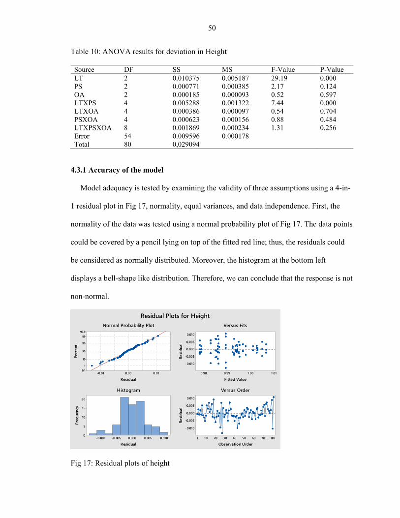
50

Table 10: ANOVA results for deviation in Height

Source DF SS MS F-Value P-Value LT 2 0.010375 0.005187 29.19 0.000 PS 2 0.000771 0.000385 2.17 0.124 OA 2 0.000185 0.000093 0.52 0.597 LTXPS 4 0.005288 0.001322 7.44 0.000 LTXOA 4 0.000386 0.000097 0.54 0.704 PSXOA 4 0.000623 0.000156 0.88 0.484 LTXPSXOA 8 0.001869 0.000234 1.31 0.256 Error 54 0.009596 0.000178 Total 80 0,029094

4.3.1 Accuracy of the model

Model adequacy is tested by examining the validity of three assumptions using a 4-in-

1 residual plot in Fig 17, normality, equal variances, and data independence. First, the

normality of the data was tested using a normal probability plot of Fig 17. The data points

could be covered by a pencil lying on top of the fitted red line; thus, the residuals could

be considered as normally distributed. Moreover, the histogram at the bottom left

displays a bell-shape like distribution. Therefore, we can conclude that the response is not

non-normal.

Fig 17: Residual plots of height

0.010.00-0.01

99.999

90

50

10

10.1

Residual

Perc

ent

1.011.000.990.98

0.010

0.005

0.000

-0.005

-0.010

Fitted Value

Resi

dual

0.0100.0050.000-0.005-0.010

20

15

10

5

0

Residual

Freq

uenc

y

80706050403020101

0.010

0.005

0.000

-0.005

-0.010

Observation Order

Resi

dual

Normal Probability Plot Versus Fits

Histogram Versus Order

Residual Plots for Height

51

The plot in Fig 17 is appropriate if you know the order in which the data is collected.

Except few residuals, we could conclude that data meets independence assumption. From

the versus-fits plot, the assumption is satisfied since the residual data had a random

spread, except for a couple of outliers left to the center but they don’t seem to follow a

specific pattern, so the independence assumption cannot be rejected.

4.3.2 Main effect and interaction plots

Having identified the significant factors, the next step is to determine optimal setting

of the factors. Main effects and interaction plots will assist us in finding the optimal level

of significant factors on the mean response, i.e., deviation in height. Fig 18 illustrates the

main effect plots of all the three factors on the mean response of height. From ANOVA

table, we observed that the factor LT has significant effect on height. We need points

closer to zero on the graph indicating the minimum deviation from target value.

Fig 18: Main effects plot of factors for deviation in height (%H)

Looking at main effects in Fig 18, we see that the least deviation in height is observed

at 0.1mm of layer thickness.

52

Fig 19: Interaction plot of factors for deviation in height

Fig 19 shows the two-way interaction plot of the factors for the height. The interaction

LT X PS is presented at the top right part of Fig 19. The lowest deviation occurs at

0.1mm of layer thickness and 80mm/sec of printing speed. As orientation angle alone has

no significant effect, any level can be used with above optimal levels. Final optimal

levels of significant factors for height are 0.1mm, 80mm/sec, any level of OA.

The optimal levels of LT and PS from main effect plots are 0.1mm and 60mm/sec

respectively, similarly interaction effect LT X PS has 0.1mmx80mm/sec as the optimal

level. With LT, and LT X PS as the significant factors, the regression equation reduces

to:

Deviation from height = 0.008654 - 0.008543 A1 - 0.00135 A1B2

53

4.4. Optimal factor determination for width

Factors effecting width will only be discussed this section. Before ANOVA test,

normality check of the data is performed by Anderson-Darling test in Fig 20. With

regards to the p-value (p-value=0. 689) in Fig 20, we cannot conclude that the data is not

normally distributed in 95% confidence level.

Fig 20: Normality test for width

Our null hypothesis is that all the factors and their interactions do not have significant

effects on deviation in width. The ANOVA results are represented in the Table 11.

Table 11: ANOVA results for deviation in Width

Source DF SS MS F-Value P-Value LT 2 0.001237 0.000618 3.29 0.045 PS 2 0.002143 0.001072 5.70 0.006 OA 2 0.000299 0.000150 0.80 0.456 LTXPS 4 0.002614 0.000653 3.47 0.013 LTXOA 4 0.000912 0.000228 1.21 0.316 PSXOA 4 0.000503 0.000126 0.67 0.617 LTXPSXOA 8 0.006638 0.000830 4.41 0.000 Error 54 0.010155 0.000188 Total 80 0.024501

From Table 11, we observe that the main effect A (p-value = 0.045), B (p-value =

0.006), interaction effect AXB (p-value = 0.013) and three-way interaction effect

0.420.410.400.390.380.370.360.350.340.33

99

95

90

80

7060504030

20

10

5

1

Mean 0.3857StDev 0.01496N 46AD 0.262P-Value 0.689

Widthh

Perc

ent

Probability Plot of WidthhNormal

54

AXBXC (p-value = 0.00) have significant effects on the deviation in width. The rest of

the factors do not have significant effects on the response based on the statistical

evidence.

4.4.1. Accuracy of the model

The model accuracy is evaluated in terms of normality, equal variance, and

independence assumption of the residuals. In Fig 21, normal probability plot (at the top

left of the graph) shows a smooth curve but no outliers, significant gaps or clear tails.

Additionally, the histogram, at the bottom left displays a bell-shaped distribution. Thus,

the normality assumption for the residuals is satisfied.

Fig 21: Residual plots for width

Like previous cases, the assumption in this case is satisfied since the residual data had

a random spread, except for a couple of minor outliers. In residual vs order graph, the

data on left side of the graph is above the center line whereas the data on the right side is

mostly below the center line but no regular trend.

0.040.020.00-0.02-0.04

99.999

90

50

10

10.1

Residual

Perc

ent

0.4000.3750.350

0.04

0.02

0.00

-0.02

-0.04

Fitted Value

Resi

dual

0.0320.0160.000-0.016-0.032

40

30

20

10

0

Residual

Freq

uenc

y

80706050403020101

0.04

0.02

0.00

-0.02

-0.04

Observation Order

Resi

dual

Normal Probability Plot Versus Fits

Histogram Versus Order

Residual Plots for Width

55

4.4.2 Main effect and interaction plots

Having identified the significant factors, the next step is to determine optimal setting

of the factors. Main effects and interaction plots will assist us in finding the optimal level

of significant factors on the mean response, i.e., deviation in width. Fig 22 illustrates the

main effect plots of all three factors on the mean response of width. Factor A and Factor

B have significant main effects on the response. The lowest point on the graph indicates

less deviation from the response; therefore, the factor levels are determined by

considering the minimum deviation point.

Fig 22: Main effects plot of factors for deviation in width(%W)

Looking at main effect plots Fig 22, we see that the lowest point of deviation is found

at 0.2mm of layer thickness and 60mm/s of printing speed.

56

Fig 23: Two-way interaction plot of factors for deviation in width

According to the two-way interaction plot of LTXPS in Figure 23, i.e., top right part

of the above graph, the lowest deviation occurs at 0.2 mm of layer thickness and

60mm/sec of printing speed.

Fig 24: Three-way interaction plot for deviation in width

57

Since there is a three-way interaction, the optimal factor levels could not be decided

by main effects and two-way interaction plots, three-way interaction plot should also be

considered. In Fig 24, the optimal factor levels that satisfy minimum deviation for width

are 0.2mm layer thickness, 60mm/sec printing speed, and 00 orientation angle.

The predicted mean response at the optimal condition is estimated only from the

significant main or interaction effects. The selection of factor levels to be used in the

prediction equation is dependent on the nature of chosen quality characteristic for the

experiment. The design model equation for this study reduces to:

Yijk = µ + Aj + Bi + ABik + ABCijk + 𝜀ijk.

With LT, PS, LT XPS and LT X PS X OA as the significant factors, the regression

equation reduces to:

Deviation from width = 0.01773 - 0.00947A2 - 0.00804B1 - 0.00709 A2B1 - 0.00254A2B1C1

4.5 Optimal factor determination for middle height

Factors/combinations affecting middle height will only be discussed in this section.

First, we perform a normality test to check if the normality assumption of the data is

satisfied. With p-value of 0.07, we can conclude that data is normal at 0.1 significance

level. Our hypothesis is that all the factors and their interactions might have significant

effects on the deviation in middle height. In 95% confidence, any factor with p-value less

than or equal to 0.05 is considered to have a significant effect on the output. The

ANOVA results are represented in Table 12.

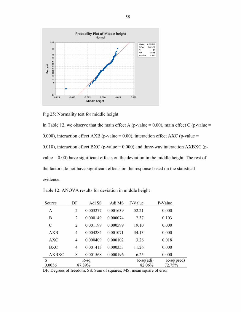
58

Fig 25: Normality test for middle height

In Table 12, we observe that the main effect A (p-value = 0.00), main effect C (p-value =

0.000), interaction effect AXB (p-value = 0.00), interaction effect AXC (p-value =

0.018), interaction effect BXC (p-value = 0.000) and three-way interaction AXBXC (p-

value = 0.00) have significant effects on the deviation in the middle height. The rest of

the factors do not have significant effects on the response based on the statistical

evidence.

Table 12: ANOVA results for deviation in middle height

Source DF Adj SS Adj MS F-Value P-Value

A 2 0.003277 0.001639 52.21 0.000

B 2 0.000149 0.000074 2.37 0.103

C 2 0.001199 0.000599 19.10 0.000

AXB 4 0.004284 0.001071 34.13 0.000

AXC 4 0.000409 0.000102 3.26 0.018

BXC 4 0.001413 0.000353 11.26 0.000

AXBXC 8 0.001568 0.000196 6.25 0.000 S R-sq R-sq(adj) R-sq(pred) 0.0056 87.89% 82.06% 72.75%

DF: Degrees of freedom; SS: Sum of squares; MS: mean square of error

0.0500.0250.000-0.025-0.050-0.075

99.9

99

9590

80706050403020

105

1

0.1

Mean 0.001716StDev 0.01323N 81AD 0.688P-Value 0.070

Middle height

Perc

ent

Probability Plot of Middle heightNormal

59

Fig 26: Pareto chart of standardized effects for middle height

On the Pareto chart in Fig 26, bars that cross the reference line are statistically

significant. In the above Pareto chart, the bars that represent factors A, C, AB, AC, BC &

ABC cross the reference line that is at 2.005. These factors are statistically significant at

the 0.05 level with the current model terms.

4.5.1. Accuracy of the model

The normality of the data was tested using a normal probability plot (bottom left of

Fig 27) and the Anderson-Darling test. This plot shows no outliers, significant gaps or

clear tails, thus the normality assumption is satisfied.

In this case, the assumption of constant variance is obviously good because the

residual data had a nice random spread, except few outliers on the left side of the plot.

From the versus order plot (Fig 27), we can say that there are three points that have

extended a little far when compared to other residuals, thus independence assumption is

satisfied as most of the points remain intact with respect to center line. After checking the

normality, constant variance, and independence of the errors, it has been concluded that

the model is adequate.

Term

B

AC

ABC

BC

C

AB

A

9876543210

A AB BC C

Factor Name

Standardized Effect

2.005

Pareto Chart of the Standardized Effects(response is Middle height, α = 0.05)

60

Fig 27: Residual plots for middle height

4.5.2 Main effect and interaction plots

Having identified the significant factors, the next step is to determine the optimal

setting of the factors. Main effects and interaction plots will assist us in finding the

optimal level of significant factors on the mean response, i.e., deviation in middle height.

Fig 28 illustrates the main effect plots of all the three factors on the mean response of

middle height. Main effects LT and OA have significant effect on the response. The

lowest point that is close to zero on the graph indicates less deviation of the response. In

Fig 28, the factor levels that achieves minimum deviation from the middle height

according to the main effect plots are circled.

0.010.00-0.01-0.02-0.03

99.999

90

50

10

10.1

Residual

Perc

ent

0.020.00-0.02-0.04

0.01

0.00

-0.01

-0.02

-0.03

Fitted Value

Resi

dual

0.010.00-0.01-0.02

48

36

24

12

0

Residual

Freq

uenc

y

80706050403020101

0.01

0.00

-0.01

-0.02

-0.03

Observation OrderRe

sidu

al

Normal Probability Plot Versus Fits

Histogram Versus Order

Residual Plots for Middle height

61

LT PS OA

Fig 28: Main effects plot of factors for middle height

In Fig 28, we see that the minimum deviation in middle height is observed at level 3

of layer thickness i.e., 0.3mm and for factor C, lowest point at observed at an orientation

angle of 900. The point is circled for easy observation. Factor B does not have any

significant effect on the deviation from middle height.

Fig 29: Two-way interaction plot of factors for middle height

62

In Fig 29, for the two-way interaction LTXPS, the lowest deviation occurs at 0.1 mm

of layer thickness and 100mm/sec of printing speed. For two-way interaction of PSXOA,

the lowest deviation occurs at 80 mm/sec of printing speed and 00 of orientation angle.

For two-way interaction of LTXOA, a lowest deviation occurs at the 0.1 mm of layer

thickness and 450 of orientation angle. The lowest deviation points of all interactions are

circled for easy observation in Fig 30.

Fig 30: Three-way interaction plot of middle height

Three-way interaction plot in Fig 30 is also checked in order to determine the optimal

factor levels. In review of the results of the three-way interaction, the least deviation is

obtained at 0.3mm, 80mm/sec, 00.

The predicted mean response at the optimal condition is estimated only from the

significant main or interaction effects. With LT, OA, LTXPS, LTXOA, PSXOA and

LTXPSXOA as the significant factors, the regression equation reduces to:

63

Deviation from middle height = 0.02763 - 0.00947A3 – 0.00267C3

- 0.00426A2B1- 0.00709A3C3 - 0.00105B2C1 - 0.00436A3B2C1

4.6 Surface roughness

Factors/combinations affecting surface finish will only be discussed in this section.

Our hypothesis is that all the factors and their interactions might have significant effects

on the deviation in surface finish. Any factor with p-value less than or equal to 0.05 is

considered to have a significant effect on the output in 95% confidence. The ANOVA

results are represented in Table 13. With regards to adjusted R2 , 76.45% of variation on

the response, i.e., the deviation in surface finish can be explained by our model.

Table 13: ANOVA results for deviation in surface roughness

Source DF Adj SS Adj MS F-Value P-Value

LT 2 5321.9 2660.94 54.03 0.000

PS 2 3977.7 1988.85 40.38 0.000

OA 2 21.7 10.85 0.22 0.803

LTXPS 4 1917.4 479.35 9.73 0.000

LTXOA 4 594.9 148.73 3.02 0.027

PSXOA 4 558.1 139.53 2.83 0.034

LTXPSXOA 8 1528.9 191.11 3.88 0.001

S R-sq R-sq(adj)

7.01789 84.73% 76.45% DF: Degrees of freedom; SS: Sum of squares; MS: a mean square of the error

In Table 13, we observe that all the combinations of factors have significant effects on

the surface finish except for the main effect of the orientation angle.

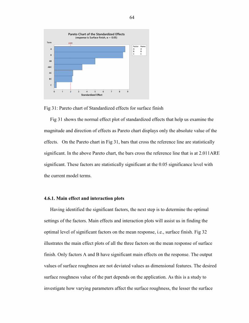
64

Fig 31: Pareto chart of Standardized effects for surface finish

Fig 31 shows the normal effect plot of standardized effects that help us examine the

magnitude and direction of effects as Pareto chart displays only the absolute value of the

effects. On the Pareto chart in Fig 31, bars that cross the reference line are statistically

significant. In the above Pareto chart, the bars cross the reference line that is at 2.011ARE

significant. These factors are statistically significant at the 0.05 significance level with

the current model terms.

4.6.1. Main effect and interaction plots

Having identified the significant factors, the next step is to determine the optimal

settings of the factors. Main effects and interaction plots will assist us in finding the

optimal level of significant factors on the mean response, i.e., surface finish. Fig 32

illustrates the main effect plots of all the three factors on the mean response of surface

finish. Only factors A and B have significant main effects on the response. The output

values of surface roughness are not deviated values as dimensional features. The desired

surface roughness value of the part depends on the application. As this is a study to

investigate how varying parameters affect the surface roughness, the lesser the surface

Term

C

BC

AC

ABC

AB

B

A

9876543210

A AB BC C

Factor Name

Standardized Effect

2.011

Pareto Chart of the Standardized Effects(response is Surface finish, α = 0.05)

65

roughness values the better is the finish on the parts. In Fig 32, we see that 0.1mm of

layer thickness alone and 60mm/s of printing speed seem to have produced parts with

lesser surface roughness.

Fig 32: Main effect plots of factors for surface finish

Two-way interaction of factors has a significant effect on the surface finish. In Fig 33,

for LTXPS, 0.1 mm of layer thickness and 60mm/s of printing speed, for LTXOA,

0.1mm of layer thickness and 45 deg of orientation angle, for PSXOA, 60mm/s of

printing speed and 45 deg of orientation angle achieve minimum surface roughness.

Fig 33: Two-way interaction plot of factors for surface finish

66

Fig 34: Three-way interaction for surface finish

The lowest values of surface finish are usually desirable; the points located closer to

the 0 are considered. From Fig 34, the optimal factor levels are 0.1 mm layer thickness,

100mm/s printing speed and 450 orientation angle. As only the factor C doesn’t have any

effect on surface finish, the model design equation reduces to:

Yijk = µ + Ai s Bk + ABij + ACik + BCjk + ABCijk + 𝜀ijk

Surface finish = 0.001716+ 0.002580 A1 - 0.000605 B1- 0.01391 A1B1 - 0.00362 A1C2

+ 0.00568 B1C2 - 0.00738 A1B2C3

4.7 Control charts

Control charts are plotted from the data of 30 parts to study how a process changes

over time as the data will be plotted in a timely manner. The optimal level of factors

obtained from ANOVA analysis are used to print another 30 parts to test if the process is

in statistical control. Table 14 shows the measured height values of 30 parts. A control

0.30.20.1

48

36

24

12

0

0.30.20.1

48

36

24

12

0

0

A

Mea

n of

Sur

face

fini

sh45

90

6080

100

B

Line Plot of Mean( Surface finish )

Panel variable: C

67

chart always has a central line for the average, an upper line for the upper control limit

(UCL) and a lower line for the lower control limit (LCL) [60]. 𝑋chart is one of the most

common chart to monitor the change on the average of the process and the central

tendency. If the process is under control, which means that the process is capable of

producing an acceptable quality of interest, we expect the mean of the process to range

between upper control limit (UCL) and lower control limit (LCL) of the 𝑋 chart. If the

sample mean 𝑋 will fell beyond the control limits, the process average for the specified

dimension is changed, and the process is incapable of printing the parts under desired

tolerances. UCL and LCL of the 𝑋 chart can be calculated as 𝑈𝐶𝐿 = 𝜇 + 𝑘√

and 𝐿𝐶𝐿 =

𝜇 − 𝑘√

, where 𝜇 is the process mean, 𝜎 is the process standard deviation, n is the size of

the sample which is taken to monitor if the process is in control, and k is the control

limits distance from the process mean. A common choice for k is 3. The difference

between a run chart and a control chart is that the run chart can help you spot upward and

downward trends but lack the benefit of statistical control limits. However, a control

chart plots a single line of data over time and it includes upper and lower control limit

lines with a centerline.

68

Table 14: Height measurement of 30 parts

Sample no Height (mm) 1 0.998 2 0.999 3 0.998 4 0.996 5 0.997 6 1.000 7 1.001 8 1.006 9 1.002

10 1.000 11 1.003 12 1.000 13 1.001 14 1.009 15 1.000 16 0.998 17 1.002 18 0.992 19 0.998 20 1.000 21 0.999 22 1.000 23 1.000 24 1.007 25 1.002 26 1.000 27 1.003 28 0.998 29 1.003 30 0.999

Fig 35 shows the control chart of height measurement for 30 parts.

69

Fig 35: Control chart for the height measurements of 30 parts (UCL – 1.0101, LCL –

0.9904)

The purpose of a control chart is to monitor a process for the special causes of

variation and to remove them when they occur. From Fig 34, the green line shows the

average of the process. The process is under control because the sample averages lay

between UCL and LCL and also they are equally distributed between UCL and average

and the LCL and the average.

4.8 Process Capability Analysis

We have observed the factors/combination of factors that have significant effects on

the response parameters based on ANOVA and main effects/interaction plots. In this

section, we finalize the optimal levels of factors to print more parts to conduct capability

analysis. The purpose of capability analysis is to check if the process is within the

statistical control and the process is capable of meeting production specifications. Of all

70

the response parameters available, optimal levels of factors having significant effects on

height are considered to print 30 parts.

Recalling the analysis discussion of height, the optimal levels of factors from the main

effect and interaction plots are 0.1mm of layer thickness, 80mm/s of printing speed. As

the orientation angle doesn’t have a significant effect on the height, any level of

orientation angle can be used. Therefore, horizontal orientation i.e., 00 has been the

chosen level.

4.8.1 Capability Studies

No two products are alike as the processes have many sources of variability. Different

sources cause different changes - some cause short term, piece-to-piece and some cause

changes over a long period. There are two types of causes responsible for variation,

common causes, and special causes. Common causes produce a stable distribution in the

system due to which the process is said to be in a state of statistical control. It affects the

process output in predictable ways. Special causes refer to factors causing variation that

affect only some of the process output in an intermittent and unpredictable way.

Capability must be less than the tolerance to be acceptable for the production. If no

special cause variation is found to be present, statistical process control (SPC) helps

define the capability of the stable process to judge whether it is operating at an acceptable

level. A process will produce conforming products as long as it remains in statistical

control.

71

The first step was to find the optimal level of factors capable of giving accurate results

which are discussed in chapters 1 and 2. We printed 30 parts at optimal level of factors-

0.1mm layer thickness, 80mm/s printing speed, and 00 orientation angle. Ppk (potential

process capability) accounts for the overall variation of all measurements taken and it

includes both the variation within subgroups and also the shift and drift between them.

Capability analysis was conducted to determine the values of Cpk and Ppk, which are

desired to be 1.33 or higher. Cpk is an index (a simple number) that measures how close a

process is running to its specification limits, relative to the natural variability of the

process. Cpk measures how close you are to your target and how consistent you are to

around your average performance [60]. Ppk basically tries to verify the sample we

generated from the process is capable to meet customer requirements. A capability

analysis is conducted using the MINITAB software to find if the process is in statistical

control. Fig 36 shows the capability analysis of height measurement of 30 PLA parts.

Fig 36: Capability histogram of 30 parts for height

Cpk values of 1.33 or greater are considered to be industry benchmarks [60]. By

observing the Fig 35, Cpk and Ppk values are greater than 1.33, this process will produce

1.0201.0141.0081.0020.9960.9900.984

LSL 0.98Target *USL 1.02Sample Mean 1.0006Sample N 30StDev(Overall) 0.00408192StDev(Within) 0.00351553

Process Data

Pp 1.63PPL 1.68PPU 1.58Ppk 1.58Cpm *

Cp 1.90CPL 1.95CPU 1.84Cpk 1.84

Potential (Within) Capability

Overall Capability

PPM < LSL 0.00 0.22 0.00PPM > USL 0.00 1.00 0.02PPM Total 0.00 1.23 0.02

Observed Expected Overall Expected WithinPerformance

LSL USLOverallWithin

72

conforming products as long as it remains in statistical control. When a process is in

statistical control, it means that the adopted procedure is better for prototyping and also

for the new product development, for which the cost of production for dies and other

tooling is more expensive (like for biomedical applications) [61]. In the context of quality

control, PPM stands for the number of parts per million that lie outside the tolerance

limits. Cpk 1.00 means that 2700 PPM (0.27%) of the manufactured parts are out of

tolerance, while Cpk 1.33 means that 63 PPM (0.0063%) are rejected.

73

CHAPTER 5. CONCLUSION

The main objective of this thesis is to investigate the effect of factors on the

dimensional features and surface finish of PLA parts printed using FFF technology.

Literature review was done on studies that focused on factors affecting the dimensional

accuracy and surface roughness of 3D printed parts. The review included different AM

technologies, materials, part geometry, process parameters and different experiment set

up. We chose FFF technology to print PLA parts (dog bone shaped specimen) with layer

thickness, printing speed and orientation angle as the process parameters with three levels

each. The optimal level of factors obtained from the experiment are used to print some

more parts to check whether the process is in control. Then capability analysis is

conducted to determine if the process can produce consistent conforming results. As a

part of the literature review, extensive research was done before setting up an experiment.

Various studies considering variability in dimensional accuracy, surface finish,

mechanical properties, DOE’s, and different experiment strategies were thoroughly

reviewed. A literature review of different AM technologies and workable materials were

very useful in setting up the experiment.

After an intensive literature review, we could conclude that layer thickness, fill angle,

shell thickness, printing speed, orientation angle, AM technology, type of response

parameters, type of material influenced the output parameters of printed parts such as

dimensional accuracy. We attempted to combine most common factors from above which

have not been done before to see if one factor might effect other factors i.e., to see if they

are dependent on each other. Layer thickness, printing speed, and orientation angle are

74

the factors that have been considered with three levels each in this study and are

replicated thrice to study the consistency of the results. A full factorial DOE experiment

was set up to investigate the effects of process parameters individually and in

combination with rest of the factors. The output of this experiment considered the effect

of these factors on dimensional accuracy and surface finish of parts built with PLA

material(polymer) using FFF technology. Each set of experiments was replicated thrice,

yielding 81 runs/prints.

As we focus on dimensional accuracy, measured values were subtracted from the

desired nominal values and presented in Table 7. Considering “smaller the better” quality

characteristics, the deviation is minimized to be able to comment on the effectiveness of

the process parameters. We conclude that the 0.3mm layer thickness, 60mm/sec printing

speed, and 450 orientation angle are the optimal levels for overall length. For height,

0.1mm layer thickness, 80mm/sec printing speed, and any level of orientation angle are

found to be the optimal levels. For width, 0.2mm layer thickness, 60mm/sec printing

speed and 00 orientation angle and for middle height, 0.3mm layer thickness, 80 mm/sec

printing speed and 00 orientation angle are the optimal levels at which least deviation

from the targeted values is observed.

Apart from the dimensional accuracy, the surface finish of the parts is measured and

almost all the factors and their combinations have significant effects on the response

parameter. An in-depth study and understanding are required to decide the levels of

factors to achieve the desired accuracy in surface finish. For this particular response

75

parameter, the values are not subtracted from any nominal value, because the parts are

tensile testing specimens and they do not have a standard finish specification to get the

deviated values. As such we just calculated how the values are affected by different

levels of factors. From the response values of surface finish, we desired the least surface

roughness values to determine the significant factors. The ideal factors in this study to

achieve better surface finish is 0.1 mm layer thickness, 100 mm/s printing speed and 450

orientation angle.

After finding the significant factors and their levels for each response parameter, we

printed 30 more parts to conduct capability studies and plot control charts to see the if the

process with our concluded optimal levels will be in statistical control and capable of

producing parts within specifications. We worked on parts focusing on height as the

response parameter with optimal levels as 0.1mm layer thickness, 80mm/s of printing

speed and 00 orientation angle. MINITAB software was used to conduct the process

capability studies and we were able to achieve Cpk and Ppk values higher than 1.33

implying that the optimal levels we found were responsible for the process to be stable

and acceptable. The control chart shows that the measured height values are within the

upper control and lower control limits.

PLA parts are not just limited to prototypes, they have wide range of applications.

Some of them include plastic films, bottles and biodegradable medical devices like

screws, pins, rods. Also, PLA contracts under heat, so it can be used as shrink material.

Therefore, experimental studies on PLA will provide better understanding of various

design applications. Design of experiments are used to design an experiment with

76

different variables to study their effect on the desirable output parameters. Once you

understand the effect of factors, you optimize the experiment to prevent the variability

caused by those factors. Process capability studies are conducted to check the consistency

in bulk productions. The samples considered in this study may be different from actual

requirement of samples in an industry. To test for accuracy and consistency of the results,

capability analysis is conducted on the parts produced with optimal levels of factors from

DOE. Work done as a part of this thesis is useful and can be applicable in different

industrial sectors. The fact that it considers multiple factors and studies their effect on the

output makes it applicable in real life complex manufacturing problems.

To optimize all the response parameters at once, one can extend this study by

generating and minimizing the mathematical equations that incorporate the absolute

deviated values of all the response parameters. Also, one can choose complex part

geometry e.g., holes, threads, curvy surfaces etc., that might vary with different levels of

factors and investigate how different the effects when compared to linear parts.

77

References 1. Ligon, S. C., Liska, R., Stampfl, J., Gurr, M., & Mülhaupt, R. (2017). Polymers

for 3D printing and customized additive manufacturing.

2. Lieneke, T., Denzer, V., Adam, G. A., & Zimmer, D. (2016). Dimensional tolerances for additive manufacturing: Experimental investigation for Fused Deposition Modeling. Procedia CIRP, 43, 286-291.

3. Gu, P., & Li, L. (2002). Fabrication of biomedical prototypes with locally controlled properties using FDM. CIRP Annals-Manufacturing Technology, 51(1), 181-184.

4. Fahad, M., & Hopkinson, N. (2017). Evaluation and comparison of the geometrical accuracy of parts produced by sintering-based additive manufacturing processes. The International Journal of Advanced Manufacturing Technology, 88(9-12), 3389-3394.

5. Ippolito, R., Iuliano, L., & Gatto, A. (1995). Benchmarking of rapid prototyping techniques in terms of dimensional accuracy and surface finish. CIRP Annals-Manufacturing Technology, 44(1), 157-160

6. Singh, R. (2014). Process capability analysis of fused deposition modeling for plastic components. Rapid Prototyping Journal, 20(1), 69-76 Das, P., Chandran, R., Samant, R., & Anand, S. (2015). Optimum part build orientation in additive manufacturing for minimizing part errors and support structures. Procedia Manufacturing, 1, 343-354.

7. Nidagundi, V. B., Keshavamurthy, R., & Prakash, C. P. S. (2015). Studies on parametric optimization for fused deposition modeling process. Materials Today: Proceedings, 2(4-5), 1691-1699.

8. Vishwas, M., & Basavaraj, C. K. (2017). Studies on Optimizing Process Parameters of Fused Deposition Modelling Technology for ABS. Materials Today: Proceedings, 4(10), 10994-11003.

9. Anitha, R., Arunachalam, S., & Radhakrishnan, P. (2001). Critical parameters influencing the quality of prototypes in fused deposition modeling. Journal of Materials Processing Technology, 118(1-3), 385-388.

10. Bakar, N. S. A., Alkahari, M. R., & Boejang, H. (2010). Analysis of fused deposition modeling performance. Journal of Zhejiang University-Science A, 11(12), 972-977.

11. Frazier, W. E. (2014). Metal additive manufacturing: a review. Journal of Materials Engineering and Performance, 23(6), 1917-1928.

12. Murr, L. E., Gaytan, S. M., Ramirez, D. A., Martinez, E., Hernandez, J., Amato, K. N., & Wicker, R. B. (2012). Metal fabrication by additive manufacturing using

78

laser and electron beam melting technologies. Journal of Materials Science & Technology, 28(1), 1-14.

13. B. Valentan et al (2013) Processing poly (ether ether ketone) on a 3d printer for thermoplastic modeling Materiali Technologies, 47 (6), pp. 715-721

14. Stansbury, J. W., & Idacavage, M. J. (2016). 3D printing with polymers: Challenges among expanding options and opportunities. Dental Materials, 32(1), 54-64.

15. Dawoud, M., Taha, I., & Ebeid, S. J. (2016). Mechanical behavior of ABS: An experimental study using FDM and injection molding techniques. Journal of Manufacturing Processes, 21, 39-45.

16. Górski, F., Kuczko, W., & Wichniarek, R. (2013). Influence of process parameters on the dimensional accuracy of parts manufactured using Fused Deposition Modelling technology. Advances in Science and Technology Research Journal, 7(19), 27-35.

17. Dul, S., Fambri, L., & Pegoretti, A. (2016). Fused deposition modeling with ABS–graphene nanocomposites. Composites Part A: Applied Science and Manufacturing, 85, 181-191.

18. Moroni, G., Syam, W. P., & Petro, S. (2014). Towards early estimation of part accuracy in additive manufacturing. Procedia CIRP, 21, 300-305.

19. Hällgren, S., Pejryd, L., & Ekengren, J. (2016). 3D data export for Additive Manufacturing-improving geometric accuracy. Procedia CIRP, 50, 518-523.

20. Žarko, J., Vladić, G., Pál, M., & Dedijer, S. (2017). Influence of printing speed on the production of embossing tools using FDM 3d printing technology. Journal of Graphic Engineering and Design, 8(1), 19.

21. Galantucci, L. M., Lavecchia, F., & Percoco, G. (2009). An experimental study aiming to enhance the surface finish of fused deposition modeled parts. CIRP Annals, 58(1), 189-192.

22. Surface roughness estimation for FDM systems - Behnam Nourghassemi – Master’s thesis, A thesis presented to Ryerson university.

23. Garg, A., Bhattacharya, A., & Batish, A. (2016). On surface finish and dimensional accuracy of FDM parts after cold vapor treatment. Materials and Manufacturing Processes, 31(4), 522-529.

24. Sheydaeian, E., Fishman, Z., Vlasea, M., & Toyserkani, E. (2017). On the effect of throughout layer thickness variation on properties of additively manufactured cellular titanium structures. Additive Manufacturing, 18, 40-47.

79

25. B.Sagomonyants, K. B., Jarman-Smith, M. L., Devine, J. N., Aronow, M. S., & Gronowicz, G. A. (2008). The in vitro response of human osteoblasts to polyetheretherketone (PEEK) substrates compared to commercially pure titanium. Biomaterials, 29(11), 1563-1572.

26. Das, P., Chandran, R., Samant, R., & Anand, S. (2015). Optimum part build orientation in additive manufacturing for minimizing part errors and support structures. Procedia Manufacturing, 1, 343-354.

27. Kurtz, S. M., & Devine, J. N. (2007). PEEK biomaterials in trauma, orthopedic, and spinal implants. Biomaterials, 28(32), 4845-4869.

28. Huang, S. H., Liu, P., Mokasdar, A., & Hou, L. (2013). Additive manufacturing and its societal impact: a literature review. The International Journal of Advanced Manufacturing Technology, 67(5-8), 1191-1203.

29. Vaezi, M., & Yang, S. (2015). Extrusion-based additive manufacturing of PEEK for biomedical applications. Virtual and Physical Prototyping, 10(3), 123-135.

30. A Quick history of Design of Experiments (DOE) – https://newonline courses.science.psu.edu/stat503/node/6

31. Huang, S. H., Liu, P., Mokasdar, A., & Hou, L. (2013). Additive manufacturing and its societal impact: a literature review. The International Journal of Advanced Manufacturing Technology, 67(5-8), 1191-1203.

32. Maghsoodloo, S., Ozdemir, G., Jordan, V., & Huang, C. H. (2004). Strengths and limitations of Taguchi's contributions to quality, manufacturing, and process engineering. Journal of Manufacturing Systems, 23(2), 73-126.

33. Dilberoglu, U. M., Gharehpapagh, B., Yaman, U., & Dolen, M. (2017). The Role of Additive Manufacturing in the Era of Industry 4.0. Procedia Manufacturing, 11, 545-554.

34. Masood, S. H., Mau, K., & Song, W. Q. (2010). Tensile properties of processed FDM polycarbonate material. In Materials Science Forum (Vol. 654, pp. 2556-2559). Trans Tech Publications.

35. Griffiths, C. A., Howarth, J., De Almeida-Rowbotham, G.Rees, A., & Kerton, R. (2016). A design of experiments approaches for the optimization of energy and waste during the production of parts. Journal of cleaner production, 139, 74-85.

36. Kumar, S., Kannan, V. N., & Sankaranarayanan, G. (2014). Parameter optimization of ABS-M30i Parts produced by fused deposition modeling for minimum surface roughness. International Journal of Current Engineering and Technology, 3, 93-97.

80

37. Chang, D. Y., & Huang, B. H. (2011). Studies on profile error and extruding aperture for the RP parts using the fused deposition modeling process. The International Journal of Advanced Manufacturing Technology, 53(9-12), 1027-1037.

38. Sood, A. K., Ohdar, R. K., & Mahapatra, S. S. (2010). Grey Taguchi method for improving the dimensional accuracy of FDM process. AIMS International Conference on Value-based Management, August 11-13, 2010

39. Melenka, G. W., Schofield, J. S., Dawson, M. R., & Carey, J. P. (2015). Evaluation of dimensional accuracy and material properties of the MakerBot 3D desktop printer. Rapid Prototyping Journal, 21(5), 618-627.

40. Lee, P. H., Chung, H., Lee, S. W., Yoo, J., & Ko, J. (2014, June). Dimensional accuracy in additive manufacturing processes. In ASME 2014 International Manufacturing Science and Engineering Conference collocated with the JSME 2014 International Conference on Materials and Processing and the 42nd North American Manufacturing Research Conference (pp. V001T04A045-V001T04A045). American Society of Mechanical Engineers.

41. Antony, J., Hughes, M., & Kaye, M. (1999). Reducing manufacturing process variability using experimental design technique: a case study. Integrated manufacturing systems, 10(3), 162-170.

42. Turner, B. N., & Gold, S. A. (2015). A review of melt extrusion additive manufacturing processes: II. Materials, dimensional accuracy, and surface roughness. Rapid Prototyping Journal, 21(3), 250-261.

43. Montgomery, D.C. (2009). Design and Analysis of Experiments (7th ed.). Hoboken, NJ: John Wiley and Sons Publishers. ISBN: 9780470128664.

44. Kirk, R. E. (1982). Experimental design. John Wiley & Sons, Ltd.

45. Lochner, R. H., & Matar, J. E. (1990). Designing for quality: an introduction to the best of Taguchi and western methods of statistical experimental design. Springer.

46. Giesbrecht, F. G., & Gumpertz, M. L. (2004). Completely randomized design. Planning, Construction, and Statistical Analysis of Comparative Experiments, 13-27.

47. Huynh, H., & Feldt, L. S. (1976). Estimation of the Box correction for degrees of freedom from sample data in the randomized block and split-plot designs. Journal of educational statistics, 1(1), 69-82.

48. Fraley, S., Oom, M., Terrien, B., & Date, J. Z. (2006). Design of experiments via Taguchi methods: orthogonal arrays. The Michigan chemical process dynamic and controls open text book, USA, 2(3), 4.

81

49. Wilk, M. B. (1955). The randomization analysis of a generalized randomized block design. Biometrika, 42(1/2), 70-79.

50. Tanco, M., Viles, E., Ilzarbe, L., & Álvarez, M. J. (2007, July). Manufacturing industries need Design of Experiments (DoE). In World Congress on Engineering (pp. 1108-1112).

51. Emerson, R. M. (1954). Deviation and rejection: An experimental replication. American Sociological Review, 19(6), 688-693.

52. Barlow, D. H., Andrasik, F., & Hersen, M. (2007). Single case experimental designs. London: Allyn and Bacon.

53. Chen, J., Sun, D. X., & Wu, C. F. J. (1993). A catalog of two-level and three-level fractional factorial designs with small runs. International Statistical Review/Revue Internationale de Statistique, 131-145.

54. Ahn, S. H., Montero, M., Odell, D., Roundy, S., & Wright, P. K. (2002). Anisotropic material properties of fused deposition modeling ABS. Rapid prototyping journal, 8(4), 248-257.

55. https://www.itl.nist.gov/div898/handbook/pri/section3/pri339.html

56. http://www.harrisonep.com/electropolishing-ra.html

57. Design of an experiment to analyze the effect of input parameters on thermal stress and deformation in overhanging part features created with SLM Additive manufacturing process by Albert E Patterson V.

58. Wu, H. C., & Chen, T. C. T. (2018). Quality control issues in 3D-printing manufacturing: a review. Rapid Prototyping Journal, 24(3), 607-614.

59. Han Chen (2015). A Process modeling and parameters optimization and recommendation system for Binder Jetting Additive Manufacturing Process. A thesis submitted to McGill University.

60. Wachs, S., & Wachs, A. (2011). Process Capability Indices: Common Misapplications. Manufacturing Engineering, 147(2), 10-10.

61. Barclift, M. W., & Williams, C. B. (2012, August). Examining variability in the mechanical properties of parts manufactured via polyjet direct 3D printing. In International Solid Freeform Fabrication Symposium (pp. 6-8). Austin, Texas: the University of Texas at Austin.

62. Lužanin, O., Movrin, D., & Plančak, M. (2014). Effect of layer thickness, deposition angle, and infill on maximum flexural force in FDM-built specimens. Journal for Technology of Plasticity, 39(1), 49-58.

82

63. Velineni, Anusha & Gunay, Elcin & Park, Kijung & Kremer, Gül & Schnieders, Thomas & Stone, Richard. (2018). An Investigation on Selected Factors that Cause Variability in Additive Manufacturing.