theseus: a maze-solving robot c. scott ananian and greg

Theseus: A Maze-Solving Robot

C. Scott Ananian and

Greg Humphreys

Independent Work

Presented to the

Department of Electrical Engineering

at Princeton University

Advisors:

Steve Lyon and Doug Clark

May 23, 1997

c© Copyright by C. Scott Ananian and Greg Humphreys, 2003.

All Rights Reserved

This paper represents my own work in accordance with University regulations.

Contents

1 Introduction 1

2 MicroMouse Mechanical Design 1

3 Sensors 3

3.1 Short range sensors . . . . . . . . . . . . . . . . . . . . . . . . . . 4

3.2 Long range sensors . . . . . . . . . . . . . . . . . . . . . . . . . . 6

3.3 Electronics for long range sensing . . . . . . . . . . . . . . . . . . 7

4 Hardware Platform 9

5 Algorithms 10

5.1 Traditional Algorithms . . . . . . . . . . . . . . . . . . . . . . . . 10

5.2 Maze solving . . . . . . . . . . . . . . . . . . . . . . . . . . . . . 11

5.3 Naive shortest paths through flooding . . . . . . . . . . . . . . . 12

5.4 Better flooding . . . . . . . . . . . . . . . . . . . . . . . . . . . . 14

5.5 “Oracle” path planner . . . . . . . . . . . . . . . . . . . . . . . . 15

6 A Simulator 16

6.1 Graphics . . . . . . . . . . . . . . . . . . . . . . . . . . . . . . . . 17

6.1.1 Animated vs. static . . . . . . . . . . . . . . . . . . . . . 17

6.1.2 Static simulation . . . . . . . . . . . . . . . . . . . . . . . 17

6.1.3 Real-time simulation . . . . . . . . . . . . . . . . . . . . . 18

7 Conclusion 19

A MicroMouse contest specifications 22

A.1 Maze Specifications . . . . . . . . . . . . . . . . . . . . . . . . . . 22

A.2 Mouse Specifications . . . . . . . . . . . . . . . . . . . . . . . . . 23

A.3 Contest Rules . . . . . . . . . . . . . . . . . . . . . . . . . . . . . 23

B Lexer-generator Input 26

C Ground Effect Calculations 28

D Mechanical Drawings 31

D.1 Mouse front view . . . . . . . . . . . . . . . . . . . . . . . . . . . 31

D.2 Mouse top view . . . . . . . . . . . . . . . . . . . . . . . . . . . . 32

iii

D.3 Mouse bottom view . . . . . . . . . . . . . . . . . . . . . . . . . 33

D.4 Gear train . . . . . . . . . . . . . . . . . . . . . . . . . . . . . . . 34

D.5 Long-range sensor mount . . . . . . . . . . . . . . . . . . . . . . 34

E Hardware Schematics 35

E.1 Processor interface . . . . . . . . . . . . . . . . . . . . . . . . . . 35

E.2 Analog electronics . . . . . . . . . . . . . . . . . . . . . . . . . . 36

E.3 Motor drivers . . . . . . . . . . . . . . . . . . . . . . . . . . . . . 37

E.4 Power supply . . . . . . . . . . . . . . . . . . . . . . . . . . . . . 38

iv

1 Introduction

Autonomous robotics is a field with wide-reaching applications. From bomb-

sniffing robots to autonomous devices for finding humans in wreckage to home

automation, many people are interested in low-power, high speed, reliable so-

lutions. There are many problems facing such designs: unfamiliar terrain and

inaccurate sensing continue to plague designers.

Robotics competitions have interested the engineering community for many

years. Robots compete on an international scale hundreds of times a year, in

events as varied as the annual MIT robot competition and the BEAM robotics

games in Singapore. One of the competitions with the richest history is the

MicroMouse competition. Micromice are small, autonomous devices designed

to solve mazes quickly, and efficiently. The MicroMouse competition has existed

for almost 20 years in the United States, and even longer in Japan. It has

changed little since its inception.

The goal of the contest is simple: the robot must navigate from a corner of

a maze to the center as quickly as possible. The actual final score for a robot

is primarily a function of the total time in the maze and the time of the fastest

run. MicroMouse mazes are typically designed as a lattice of square posts with

slots in the sides to accomodate modular wall units. The specifications for the

MicroMouse contest are presented in appendix A (See [3]).

Our design incorporates many of the advances in small scale robotics that

have been explored in 20 years of MicroMouse competitions. We also introduce

some features never before seen in a working design. We therefore believe that

our design is the most advanced MicroMouse ever conceived. We incorporate

sophisticated long and short range sensing mechanisms, accurate motion and

distance measurements, adaptability, high speeds, and a sophisticated, physi-

cally based algorithm for maze solving.

2 MicroMouse Mechanical Design

The MicroMouse rules are remarkably flexible with respect to mouse design; we

did considerable research into current and past international-class MicroMouse

designs in order to formulate a philosophy of design.

The most important recent advance in micromouse performance has been

Dave Otten’s development of “diagonal-capable” mice. Instead of adhering to

90-degree turns and a manhattan path, Otten’s MITEE mouse looked for op-

1

portunities to cut corners and run path diagonals. This imposes more strigent

width requirements on the mouse. We collected an exhaustive library of maze

layouts, dating from the 1st All-Japan Micromouse Contest in 1980, an in our

analysis discovered the increasing prevalence of what we dubbed “30-degree”

paths. In constrast to a diagonal path, which is constructed from a sequence of

alternating orthogonal paths (for example, “one-up, one-over”), a “30-degree”

path contains a two-to-one ratio of orthogonal segements (for example, “two-

up, one-over”). Our calculations revealed that the width requirements of a

“30-degree”-capable mouse was required to satisfy extremely tight width re-

quirements, which our completed mechanical design could not meet. We fell

back on traditional 45-degree diagonal capability, which dictated the 9cm width

of our mouse.

According the Dave Otten, the most pressing challenge to mouse design to-

day is traction control. High-power DC motors can easily outstrip the traction of

the mouse tires, leading to wheel slippage and poor performance. Robin Hartley

of New Zealand was the first to attempt to utilize a ground-effects fan to achieve

better wheel traction: the downforce generated by the fan increases the amount

of acceleration force obtainable from wheel traction. However, Hartley designed

his mouse on a large scale: a 15cm mouse diameter mouse, weighing 1.6kg, with

a fan capable of providing 2kg down force. As a result the traction benefits

did not compensate for his mouse’s poor cornering and sensing capabilities. We

performed an analysis along the lines laid out in [7], using fans from a variety

of manufacturers. For a typical example, we discovered we could increase our

traction by about 20%, if we could keep the total weight of the mouse below 200

grams. Using miniature DC brushless fans, this was possible, and we were able

to draft a mechanical design meeting our width requirements incorporating the

ground-effect fan.1 Appendix C details the mathematics supporting our claim

of efficacy.

There is no strong agreement on the advantages of two-wheeled over four-

wheeled micromice, but it was felt that a two-wheeled mouse was mechanically

simpler, and thus more likely to allow us to meet our weight requirements. Servo

inaccuracies, increased parts count, and other factors made us shy away from

four-wheeled designs.

Sensing devices have traditionally been classified as “over-the-wall” or “under-

1The fan used in the final design was a Panasonic FBK series brushless DC fan fromDigikey electronics, measuring 40mm square and 20mm deep. It develops 11.5mm H2O staticpressure.

2

the-wall.” The original micromice used the red-painted wall tops to determine

orientation, with long wing-like sensor arrays extending over the walls. More

recent designs have avoided the large moments of inertia that these extended

sensor assemblies create, and have opted instead for compact low-riding mice

which measure distances from the insides of the walls. This latter approach

was markedly superior, and permitted extremely compact designs. Sensor de-

sign will be discussed further in section 3; from the mechanical design aspect it

is only important that we decided no use optical, rather than ground-contact

(rolling) distance sensors.

The mechanical design of the mouse was completed using Pro/Engineer CAD

tools, and fabricated using computer-controlled milling machines. Appendix D

details the design. The use of computer-controlled milling machines enabled a

high degree of precision in the design; clearances as tight as one-quarter mil-

limeter were successfully utilized. Most of the components are plastic, to save

weight; the motor and bearing assemblies are aluminum for strength and rigid-

ity, and the top surface is made of aluminum to allow it to act as a heat-sink

for the power and control electronics.

3 Sensors

In order to execute these algorithms (and keep from crashing into obstacles),

the MicroMouse must be able to “see” the environment around it. There are

some very serious technical challenges associated with this task. First, we need

not only to be able to detect obstacles, but also to measure our distance from

them at very close proximities. When our mouse traverses a diagonal path, the

maximum spacing between posts is exactly 16.8√

2= 8.4

√2 ≈ 11.76cm. Because of

space constraints imposed by the sizes of our motors and batteries, the mouse is

exactly 9cm wide, which leaves 1.38cm of clearance on either side of the mouse.

At top speeds of >15 ft/sec, it is clear that we must have accurate distance

measurements at short distances in order to avoid hitting the posts.

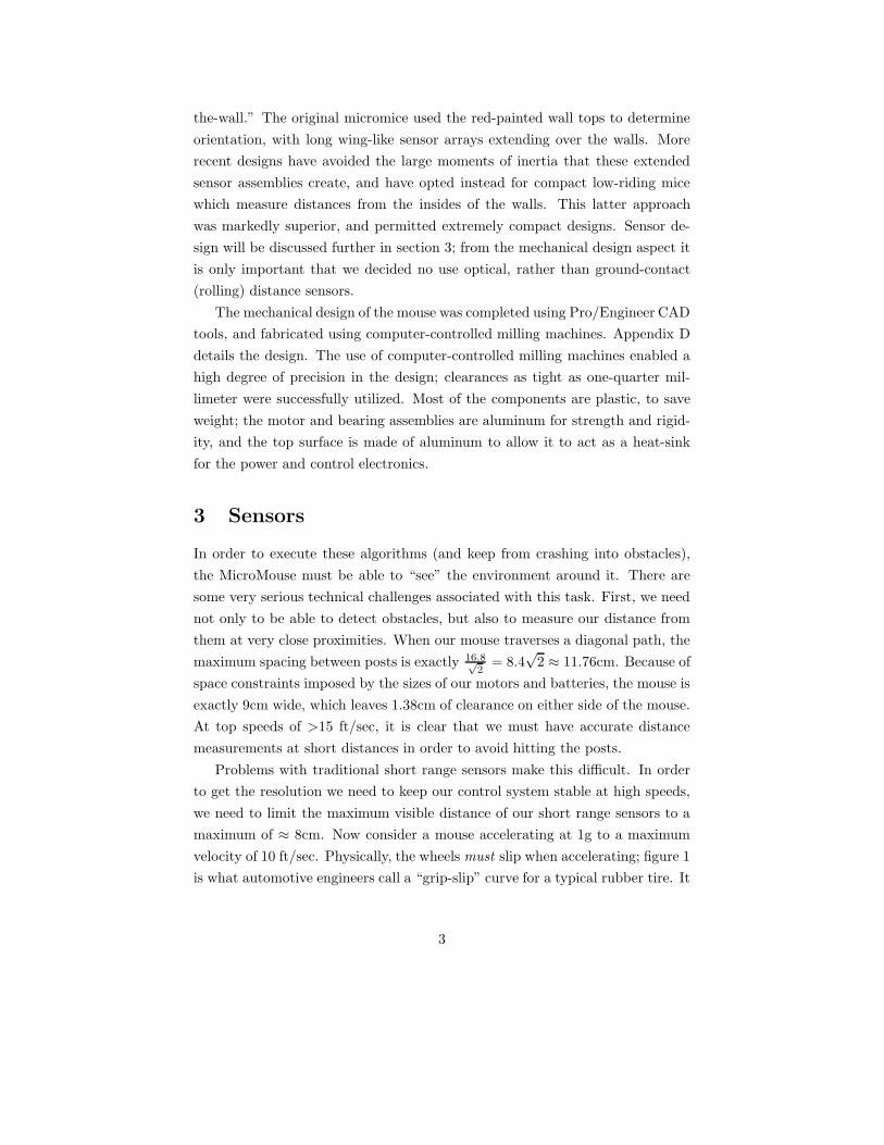
Problems with traditional short range sensors make this difficult. In order

to get the resolution we need to keep our control system stable at high speeds,

we need to limit the maximum visible distance of our short range sensors to a

maximum of ≈ 8cm. Now consider a mouse accelerating at 1g to a maximum

velocity of 10 ft/sec. Physically, the wheels must slip when accelerating; figure 1

is what automotive engineers call a “grip-slip” curve for a typical rubber tire. It

3

Gri

p

Slip

Figure 1: Grip-versus-slip curve for typical tire

is obvious that some amount of wheel slip is necessary to exert the acceleration

force. Worse, the actual grip-slip curve is dependent on floor material and thus

unknown to us—all we know about the floor is that it absorbs light. However,

we must have a reliable way to measure the distance we have traveled. It is clear,

then, that any distance measure we make can not totally rely on the motion

of the wheels or the motors. Typical advanced mouse designs get around this

problem by mounting “idler” wheels on the ground that are not powered by the

motors, but merely roll on the ground. While this solution is attractive, it uses

precious space under the mouse, and, in our design, this space is at a premium.

It was therefore necessary to design a solution on top of the mouse. This led to

the design of our long range sensing mechanisms.

3.1 Short range sensors

As discussed in the introduction to this section, our short range sensors need to

have a dynamic range of 1-8cm. To accomplish this, we use a fairly traditional

design for distance measurement. Our short range sensors use one infrared

LED and two photo-sensitive detectors, spaced a known distance apart. This

configuration is shown in figure 2.

Note that the angle of acceptance of the two detectors is very narrow, while

the angle of light given off by the LED is large. Therefore, because of the 1

r2

4

PHOTODIODE

WALL

LED

8 degrees

PHOTODIODE 8 degrees

60 degrees

Figure 2: Design for short range sensors

falloff nature of light, the quotient of the voltages produced by the two photo-

transistors will be a monotonic function that is directly related to distance. An

empirically determined lookup table will allow us to compute the actual distance

if necessary.

Another important property of this design is the fact that it is completely

insensitive to the operating environment. At startup time, we calibrate the

sensors by taking measurements of voltage readings in the contest environment.

This allows us to correct for the ambient light levels at run-time. In addition,

our two detector design has a significant advantage over the more conventional

one detector method: it is totally insensitive to the reflectivity of the surface.

Recall that MicroMouse mazes are typically designed as a lattice of square

posts with slots in the sides to accommodate modular wall units. It is well known

in the MicroMouse community that the reflectance of the walls of the maze may

not be the same as the reflectance of the posts, especially in Japanese mazes.

Many American mice have failed in Japan because their sensors got confused

when they were shining on a post. Because we are taking a quotient of two

voltages measured with a vertical displacement, as long as the reflectivity is

constant in the vertical dimension, our sensors will behave properly.

It is important to note that the above quotient is in fact proportional to

the square of the distance, which means we will get much higher resolution

measurements as the distance decreases. This is exactly the behavior we desire,

5

since it is very important to remain stable at close proximities to walls, especially

in the diagonal path case.

3.2 Long range sensors

Our long range sensor mechanisms are much more sophisticated. In order to

understand the design, it is first important to discuss how these sensors are to

be used. The long range sensors measure distance to an object that is much

farther away than can be measured by our short range sensors. However, we

expect the accuracy to be much less. The only requirements we place on our

short range sensors are that they can measure our position to within half a maze

block, or 9cm. The reason for this comes from the worst case scenario for wheel

slippage, shown in figure 3.

Figure 3: Worst case scenario for wheel slippage

Every time we pass an opening in a wall, our short range sensors will detect

this. As long as we know what block we’re in, we can update our current

absolute position with high accuracy. The worst case situation shown in figure

3 shows a maze configuration where we must speed down a long straightaway

and then make a very sharp turn somewhere in the middle. For motor control

reasons, the turn must begin before the front of the mouse crosses the opening

in the wall. Therefore, we must know where we are to within half a block, or

two things might go wrong. First, we might begin the turn at the wrong time,

hitting the wall mid-turn. Second, we might not begin braking early enough to

make the turn at all without slipping. Wheels slipping in place is a recoverable

error, but skidding around a turn poses a much harder problem.

6

To design a sensor to meet these requirements, we created a special purpose

laser range finder. Our design uses a linear triangulation method that exploits

properties of similar triangles in a way similar to the grade school method of

computing the height of a building based on its shadow. Our design is shown

in figure 4.

f

b

x

dPSD

LASER

WALL

Figure 4: A long range sensor

The spacing b between the laser and the lens is known, as is the distance

f between the lens and the rear surface (in fact, it is the focal length of the

lens). Because of this, we can compute the distance from the laser to the object

x if we can measure the displacement d of the image of the laser beam on the

rear surface. This turns out to be relatively easy; we simply use a “Position

Sensitive Detector”, or PSD. PSD’s are devices typically found in auto focus

cameras, where they are used for approximating distances to objects. This

application is very similar to what we are trying to accomplish with our long

range sensors. By focusing the image of a laser beam on the PSD, we can obtain

a fairly accurate measurement of our distance up to 5-6 feet away.

3.3 Electronics for long range sensing

The long-range sensors use sophisticated techniques to achieve maximum pos-

sible resolution. The raw sensor output is a micro-amp level current swamped

by light noise, especially 60Hz flourescent “buzz.” We modulate the laser in the

frequency-domain, and then demodulate the sensor output phase-locked to the

laser to recover the desired signal while achieving very high noise reduction. The

7

modulation frequency is 10kHz, which is as far from our 60Hz dominant noise

source as possible without running afoul of the limited high-frequency response

of the position-sensitive detector sensing element.

The first step in the signal chain is a pre-amplifier to convert the sensor

current to a voltage, amplified one million times. The output of this stage is a

nominally one-volt signal.

This signal is fed into a switched-capacitor bandpass filter. This device melds

digital and analog technology to allow filter design with excellent frequency

precision. The switched-capacitor device creates a bandpass filter using the

same frequency source as the laser modulation, so the center frequency of the

filter is guaranteed to coincide exactly with the laser modulation frequency. The

output of this stage is a small-amplitude 10kHz signal, which is then AC-coupled

to eliminate any DC bias. The bandpass filter is second order, so it reduces the

60Hz noise by more than 80dB.

This signal is fed into a demodulator, which multiplies it by a phase-corrected

version of the laser modulation to recover the signal amplitude. This signal is

low-level and contains some high-frequency noise at the modulation frequency

and higher.2

The next stage is a 3rd-order low-pass filter to remove this high-frequency

noise. This filter also amplifies the signal to the correct level for input to analog-

to-digital converter. The filter cut-off frequency is 1kHz, so the maximum signal

bandwidth is 1 sample/millisecond after passing through the filter. The 3rd

order filter attenuates the 10kHz carrier by 60dB.

The analog-to-digital conversion maintains higher than 60dB accuracy, so

the 10kHz ripple is still significant. To eliminate this effect, the two signals

from each sensor are fed into a sample-and-hold amplifier. This allows us to

sample both signals at exactly the same instant in time. Since the desired

information (distance) is a function of the ratio of the two signals, sampling

synchronously minimizes the effect of the high-frequency ripple.

The last stage allows an amplifier with gain of 4 to be inserted into the signal

chain, to enhance resolution at low signal amplitudes.

The use of a single frequency reference for the laser modulation, bandpass

filter, and demodulator allows high precision with simple circuitry. Furthermore,

the frequency generation is accomplished with a reprogrammable logic element,

so that the different signals can be phase-corrected through software.

2The switched capacitor filter also adds some 200kHz noise which will be eliminated alongwith the 10kHz modulation noise.

8

4 Hardware Platform

The electronics design centers around a Motorola MC68334 processor [4]. The

MC68334 has integrated motion-control functions which make it ideal for our

project and it’s high integration level helps keeps parts count low. It is interfaced

to 2MB of EEPROM for in-circuit reprogrammable non-volatile storage and 1M

of SRAM for data structures and stack. The BDM (Background Debugging

Mode) interface of the processor allows debugging and reprogramming [2].

The processor is interfaced with a complex analog signal chain described in

section 3.3 through the integrated A/D. Short-range and long-range sensors are

fed through analog multiplexors, sample-and-hold and variable gain amplifier

stages before being input to the A/D; battery-level and temperature signals use

the remaining channels of the integrated A/D.

Pulse-width-modulated outputs from the 68334 TPU (Time Processor Unit)

drive a pair of PALs programmed to do brushless-motor commutation. They

also generate an output signal whose frequency is proportional to commutation

speed, in order to provide a secondary velocity sensing mechanism. The com-

mutator output is fed through opto-isolators before input to an array of power

transistors, cooled by direct mounting to the aluminum mouse chassis.

A total of four reprogrammable logic devices (ispGALs) are used in the

design. This allows flexible modification to the electronics without necessitating

socketed parts or desoldering. Two are used for the motor commutation, one is

used for random processor support logic, and the last is used to generate the laser

modulation and demodulation clocks. The reprogrammable device allows us to

coalesce a long clock-divider chain into one device, as well as letting us flexibly

change the phase relationship of the modulation and demodulation clocks to

compensate for analog processing phase delays.

Power for the electronics is carefully conditions to isolate battery voltage

swings and motor transients from the sensitive digital and analog electronics.

The 12V, 2A battery pack (8 Lithium rechargable AA cells made by Tadrian

electronics) is rectified and filtered to isolate transient negative-going voltage

spikes, then down-converted to 8.0V by a pair of 1A regulators. The main

processor electronics are powered by a 5V 1A regulator from one of the 8V 1A

supplies. The other 8V 1A supply powers a second 5V 0.5A regulator feeding

the ispGALs, and also feeds the analog electronics. The 8V supply is mirrored

with a switched-capacitor voltage converted to -8V, and then the nominally

±8V supplies are down-converted to ±5V using low-noise linear regulators. The

9

output is a ±5V 100mA. Finally, a precision 3V reference (generated either by

an Analog Devices AD780AR part, or a National Semiconductor LP2950ACZ-

3.3 part) is generated from the stable analog +5V supply for use by the A/D

converter.

5 Algorithms

Traditional maze solving algorithms, while appropriate for purely software so-

lutions, break down when faced with real world constraints. When designing

software for a maze solving robot, it is important to consider many factors not

traditionally addressed in maze solving algorithms.

5.1 Traditional Algorithms

Our initial attempt at a maze solving algorithm was a traditional depth first

search. We were mainly interested in testing features of our simulator, and

wanted merely to find a path from the start to the center. Unmodified depth

first search is not applicable to a physical device, because it must backtrack

when it encounters a dead end in its search to reach its last decision point.

Except in the high school level competitions, MicroMouse mazes are almost

always constructed so that there is more than one path from the start of the

maze to the center. Therefore, depth first search fails miserably for use in a

MicroMouse competition. Although it will always find a path from the start to

the center, it will not even be the shortest path, much less the fastest.

Kruskal’s shortest path algorithm for graphs [6] can be easily modified to

solve mazes; the maze is simply represented by a graph with a node at each

cell, and links of equal weight connecting adjacent cells without a wall between

them. However, Kruskal’s algorithm suffers drawbacks, as well.

First, MicroMice do not have immediate random access to the maze config-

uration, as the mouse must explore unseen portions of the maze, which takes

time. In fact, most maze solving algorithms assume that the entire maze con-

figuration is known a priori, and that we have random access to the complete

maze configuration. Obviously, this is not the case.3 Our information about

the maze changes as we explore, so we must make certain assumptions about

unseen portions of the maze at certain steps in most algorithms.

3Actually, a team from Motorola created a mouse that extended a CCD camera overheadand performed image processing to determine the configuration of the maze before running.The mechanical overhead of the scheme ensured its failure.

10

Second, the path computed may not necessarily be the best path to choose.

Although it is true that Kruskal’s algorithm will return the shortest path, this

is not necessarily the fastest path because our mouse can accelerate and also

has cornering behavior. Therefore, we would like to favor paths that have long

straightaways, and few tight turns. Even if the maze configuration was known

a priori, the shortest path from the start to the finish may not be the fastest.

We must factor in things such as maximum acceleration, turning speed, vari-

able floor conditions, etc. This requires a sophisticated, physically based, path

planner, with the appropriate assumptions about unseen areas of the maze.

5.2 Maze solving

First, we present pseudocode for the main body of our maze solving algorithm.

procedure AlgorithmStep(path_t best_path)

{

if already in center

Take best_path back to start square

else if current position is on best_path

{

Follow best_path towards destination until in center or best_path blocked

if best_path blocked

best_path = ComputeBestPath(best_path.start, best_path.end);

AlgorithmStep(best_path)

}

else

{

new_path = ComputeBestPath(current_position, best_path);

AlgorithmStep(new_path); /* Now we know we’re on best_path */

AlgorithmStep(best_path);

}

}

Notice that the ComputeBestPath function can either compute the best path

between two points, or from a point to a path. The latter computation is simply

the minimum of all point-to-point path costs from the given point to every point

on the given path.

11

This algorithm not only finds the best path from the start to the center, but

it also deals nicely and efficiently with the fact that we do not have random

access to the maze.

In fact, this pseudocode is slightly simplified. The main code actually calls

this routine twice; once to search for the center, and once to search for the start.

When we are searching for the center of the maze, the best path variable is re-

computed at each step to go from the current position to the center, rather than

from the start to the center. This is to ensure that we find the center as quickly

as possible, in case we are unable to make a high speed run. Once the center is

found, the true best path is searched for. Another slight difference involves the

assumptions about the unseen portions of the maze. When computing the best

path between center and start, we assume that unseen portions of the maze are

open and can be traversed at high speeds. However, when computing best paths

from the current position, we make the more conservative assumption that the

space is open, but we must traverse that space at searching speed.

This is because if we are computing a best path that originates at our current

position, we intend to traverse it immediately, and we must therefore account

for entering unseen territories. However, for start-to-finish paths, we will ensure

that all blocks along the path are open, so once the path is computed and

verified as traversable, there is no longer a need to assume anything about it,

and we can traverse it at the highest speed possible. This distinction does not

matter for the simple flooding algorithm, but will come into play later once the

algorithms become more physically based.

With this algorithm, the bulk of the problem has been isolated to one routine,

called ComputeBestPath. This routine takes a start point and and end point

(and some parameters for assumptions to make), and computes the best path

between those points. The question remains then, how can we implement this

algorithm to fully encapsulate all the physical characteristics of our maze solving

device?

5.3 Naive shortest paths through flooding

Our first attempt was to use a slight modification of a shortest paths algorithm.

We call this a “flooding” algorithm. This is a simple implementation of Kruskal’s

shortest path algorithm made specific to mazes. Imagine a hose being placed

in a cell in the maze, and water being allowed to flow from a cell to a neighbor

in one unit time. A simple recursive algorithm will yield the amount of time

12

it takes for water to reach any point in the maze from any other point in the

maze, and an appropriate traversal of the matrix of flood values will yield the

shortest path.

Code for this algorithm is shown below. The flood values are represented

as a 16x16 array of integers (maze), and the wall configurations are represented

with four 16x16 boolean arrays called north, south, east, and west.

void Flood(int x, int y, int flood_val)

{

if (maze[y][x] > flood_val)

{

maze[y][x] = flood_val;

if (!east[y][x])

Flood(x+1,y,flood_val+1);

if (!west[y][x])

Flood(x-1,y,flood_val+1);

if (!north[y][x])

Flood(x,y+1,flood_val+1);

if (!south[y][x])

Flood(x,y-1,flood_val+1);

}

}

Once we have a flooding routine, it is easy to answer the question “what

is the best path from point a to point b”. We simply flood the maze starting

at b with a flood value of zero, and then traverse the maze starting at a and

following decreasing flood values until we reach b. This works because once

flooding is done, the flood value at a is exactly the length of the path from a

to b. Therefore, if we follow the flood values in a monotonic decreasing order,

we are guaranteed to reach b in exactly the minimum amount of steps. Note

that the path generated by this algorithm is not unique, as there may be several

paths from a to b with identical lengths.

Also, because we know that the center of the maze is open, the maximum

flood value for any flood in any square is 254, so we can use 255 to initialize the

flood array, and can therefore represent the entire array of flood values in 256

bytes of memory. This is because the worst case for flooding is a spiral in which

the flow has to touch every square. If our flood starts at one corner of the maze,

and spirals towards the center, it will have length 252 when it enters the center

13

of the maze. Because we know that the center is an open 2x2 square, it will take

254 steps to get to the corner of the center, not 255 in the closed-center worst

case. Therefore, if all flood values are initialized to 255, a flood value of 255

represents an unreachable portion of the maze. MicroMouse maze designers will

often put these in the maze (i.e., a fully walled off square) to test the robustness

of the MicroMouse algorithms.

Although the straightforward flooding algorithm works well for a shortest

path computation, it does not allow our mouse to take full advantage of its accel-

eration capabilities, and its ability to traverse diagonal paths without turning.

That is, because of how thin our mouse is, and the precise spacing of the sensors,

if we intend to traverse a “stairstep” pattern in the maze, we can simply turn 45

degrees and go straight without turning at all. This is a huge advantage, and is

yet another thing that MicroMouse maze designers will intentionally put in the

maze. The maze flooding algorithm is the one typically used by student mouse

projects when they are simply interested in getting something that works. It is

not a world class implementation of a physical maze solving algorithm, and we

clearly needed something better.

5.4 Better flooding

Our first attempt to account for the acceleration values was a modification to

the flooding algorithm to “weight” the flood values based on a record of how

long the water had been traveling without turning. This algorithm turned out

to be ugly to implement, but when fully functional, yielded promising results.

By creating a table lookup function based on measured acceleration values, we

were able to get a fairly accurate model of the characteristics of our mouse. This

simply required retaining state information at each cell in the graph. The state

information would store the current cost of the path, as well as the direction of

flow. This way, as the water flowed along a straight path, the added penalties

would be a function of the length of the flow.

Again, this algorithm does not deal with diagonal paths. Although our path

optimizer was able to collapse stair-step patterns in a path into a long diagonal,

it was not clear how a modification of the flooding algorithm could use the

knowledge of diagonal paths to allow water to “flow” diagonally.

Another severe disadvantage of both flooding algorithms is their large stack

requirements. Like depth first search, maze flooding is highly recursive. On a

maze that has 256 blocks, the stack requirements can quickly become unrea-

14

sonable, especially for an embedded system. The standard Computer Science

paradigm of “memory is cheap” simply doesn’t apply here. It was clear we

needed to come up with something new.

5.5 “Oracle” path planner

A software module named oracle implements our algorithm for computing the

fastest path while accounting for physical characteristics of our mouse. The

basic strategy is a textbook breadth-first search, extended with look-ahead and

pruning. The problem is that in order to compute the sequence of turns (and

thus the time required) to run a path, we need a certain amount of look-ahead.

For example, the cost to travel one square north is different if we’re describing

a straight-line path, or the top of a turn in which the next square to be visited

is to the east. It turns out that it is fairly simple to make a canonical collection

of such “turn patterns,” and efficiently search through them to discover path

cost.

This requires that we keep a certain amount of path context available. For

paths which include 45-degree turns, we need 7 unit-travel elements of context.

But the costs computed necessarily lag behind the extent of path “discovery”—

we can’t tell the cost of a turn until we’ve seen 4 blocks after the turn. Concep-

tually, we need to see enough blocks before the turn to determine the entrance

angle and enough blocks after the turn to determine the exit angle before we can

determine the angle subtended by the turn. The net result is that our computed

costs reflect the time needed to reach the mid-point of the 7 units of context.

This requires look-ahead in the standard breadth-first search algorithm; which

impacts the amount we can prune the path. We use some heuristics to eliminate

contexts which self-intersect or do other obviously incorrect things.

The only thing left is to efficiently map 7-unit “contexts” to their proper

turn costs. We have implemented a simple lexer to perform this mapping in

no more than 7 array references, with a compact 177-entry table. The base

patterns to be recognized are:

15

N-N-E-N 45-degree turn from orthogonal

N-N-E-E 90-degree turn from orthogonal

N-N-E-S-E 135-degree turn from orthogonal

N-N-E-S-S 180-degree turn from orthogonal

N-W-N-N 45-degree turn from diagonal

N-W-N-E-N 90-degree turn from diagonal

N-W-N-E-E 135-degree turn from diagonal

The patterns have been normalized so that the first direction is north. Orthogo-

nal directions are north, east, south, and west; diagonal directions are northeast,

southeast, southwest, and northwest. The lexer-generator we wrote automat-

ically generates the mirror-image and rotated versions of these patterns from

the normalized patterns. Further pattern expansion is necessary to smoothly

integrate the turn cost as the path is extended. See appendix B for the complete

lexer pattern input.

The lexer-generator creates the lexical analyzer from turn patterns. It is

extendible to accomodate the much larger library of turn patterns necessary to

properly evaluate 30-degree paths. Our lexer is provided with a set of predeter-

mined path costs for all types of patterns.

The search algorithm is optimized to grow the search tree from both the

start and goal simultaneously, to reduce the polynomial growth of cells searched.

The algorithm as implemented suffers from some search instabilities at the path

midpoint because of this optimization, as well as occasionally overly-agressive

search pruning. These trade-offs are acceptable for the performace gains they

allow.

6 A Simulator

Considering the amount of time required for the construction of the Micro-

Mouse, it was important that we understand the behavior of our algorithms

and visualize the behavior of the proposed system before the finalization of the

hardware and electronics.

To accomplish this, we created a MicroMouse simulator that accurately sim-

ulated both our algorithms and the physical characteristics of our mouse. This

simulator is highly cross-platform, and allows us to develop and debug our al-

gorithms in almost any environment.

16

6.1 Graphics

We wanted our simulations to be as graphical as possible, and to allow us to

visualize as many aspects of our system as possible. There are many issues

involved in implementing a visual simulation of a moving system, which we

discuss in this section.

6.1.1 Animated vs. static

Since we are simulating the motion of a robot in real time, obviously it would

be beneficial to have our simulation run in a graphical environment in real

time as well, to visualize the behavior of the mouse. However, since real time

graphics are notoriously system dependent, we also created a static version of

our simulator that merely dumps results to disk for later analysis.

Both methods have their advantages and disadvantages. The real-time sim-

ulator allows us to see exactly how the mouse moves while it is searching the

maze, which lets us optimize certain cases until we are satisfied that the mouse

searches in what we consider to be an intelligent way. In addition, the real-time

version can be compatible with telemetry information relayed back to the com-

puter by the mouse. This would allow us to debug high level software problems

specific to the embedded version of the algorithm. On the other hand, a com-

plete run on the real-time simulator takes considerable time, since the mouse

must animate slowly enough for the programmer to comprehend its motion

paths.

The static version allows us to make runs much more quickly, and merely

look at the path chosen by the mouse at the end of the search phase. This

method clearly has the advantage that the results can be viewed at a later

time, and that it allows more detailed analysis, since the path is not constantly

moving. However, the static version gives no insight into how the mouse arrived

at its decision of what path to take.

6.1.2 Static simulation

First, we look at the simpler case; the static version, named Frankie. In this

case, we simply want to be able to see the path that the mouse chose as the best

path through the maze. This information is not as useful as the full spectrum

of information afforded by the graphical version, but it served very well when

we were improving the algorithm for deciding which path through the maze is

17

“best”.

Another goal for Frankie was that it be completely portable to any system

that we had not written a real-time interface for, to allow us to work in any

environment that we encountered. To accomplish these goals, we chose to have

the simulator output TCL/TK code, which could be saved to a file and viewed

at a later time.

TCL is an interpreted language developed by John Ousterhout [5]. It has

been ported to many platforms, and offers a system-independent set of “widgets”

called TK, which allow the creation of graphical user interfaces in an extremely

simple, portable way. It is the perfect tool for our static graphical output.

Frankie outputs code to create a window, draw a picture of the maze in

question, and draw a long line representing the chosen path through the maze.

This output can then be saved to a file and interpreted by the TCL/TK inter-

preter, which then displays our graphics in a window, regardless of the system

we were working on. X Windows on a UNIX platform, Windows 3.1, Windows

95/NT, or Macintosh platforms are all supported by TCL/TK, thus achieving

our portability goal. We are even able to simulate our mouse’s behavior as a

web page using the TCL/TK plug in for Netscape Navigator.

6.1.3 Real-time simulation

To visualize the full behavior of our system, we needed a graphical simulator

that could animate the behavior of our mouse. In addition, we wanted a system

that would be compatible with a debugging telemetry board we designed for

the mouse. The real-time simulator, called Benji,4 runs with multiple threads

to allow this behavior.

A thread is a sequence of execution of instructions; one program can create

multiple threads, which are executed independently and either share a single

processor or can take advantage of multiple processors if they are available in

the simulator machine. Threads support the notion of “shared memory”. That

is, certain portions of memory are readable and writable by all threads within

one program. It is this shared memory feature that allowed us to create Benji.

Benji consists of two threads: one thread controlling the graphics, and one

thread controlling the motion of the mouse. The interaction between these two

threads is crucial to our design. The graphics thread is, in a sense, “dumb”. It

4Benji and Frankie were the two white mice in Douglas Adams’ The Hitchhiker’s Guide

To The Galaxy who oversaw the construction of the Earth [1].

18

doesn’t know anything about mice or physical properties or motion; all it knows

how to do is draw a picture of the world. To do this, it first draws a picture of

the maze in the window, and then looks in shared memory to find out where

to draw the mouse, and how to plot path tracking information. The structure

that holds the mouse position information is constantly being updated by the

other thread, which is simulating the motion of the mouse.

This behavior is very convenient for a number of reasons. First, it allows us to

separate the graphical user interface almost completely from the code doing the

computation. In fact, Benji and Frankie share most of their code. In addition,

it makes Benji more portable since it is very clear which portions of the code

need to be re-written for a new platform. In addition, since the graphics thread

is merely drawing whatever it finds in a shared structure, it has no knowledge

of what is making the values in that structure change. In particular, the second

thread of the application does not have to be our simulator. It can instead be

code that reads debugging information directly from the telemetry board on the

mouse, giving us a graphical representation of the mouse’s perspective on the

world. This feature allows us to determine quickly when the mouse’s internal

model of the world becomes inconsistent with the actual world.

Our first implementation of a real-time graphical engine for our simulator

was done for Silicon Graphics machines, using OpenGL. Although this version

was easy to implement and worked very well, it was not practical to cart an SGI

machine to the field where we wanted to take telemetry measurements from a

real mouse. Therefore, a second version for the Power Macintosh was written.

Versions of our simulator have also existed in various forms for the BeOS Op-

erating System, as well as Windows NT. We found that our simulator and our

separation of algorithm and visualization allowed us to critically evaluate our

choice of algorithm, as well as debug the actual code that would later run on

the embedded controller of the mouse.

7 Conclusion

MicroMouse is a prime example of an engineering challenge in which the short-

comings of theory are exposed. Many real-world constraints conspire to render

standard techniques for problem solving inappropriate. We have presented our

solutions to some of these problems.

Solving mazes is a problem that has been explored in great detail in Com-

19

puter Science, but none of the standard extant solutions were appropriate for

our problem. We have created a new maze solving technique appropriate for

use in a physical device that fully accounts for its physical characteristics. In

addition, we have created a cross platform MicroMouse development environ-

ment that facilitates investigation of new MicroMouse algorithms. Our system

shows great promise for physically correct simulation and solutions of real-world

problems that are not fully addressed by standard theoretical results.

In addition, we have created a hardware platform that is able to support

international-level MicroMouse contest competition. The cross-disciplinary na-

ture of the project has required us to learn elements of mechanical, control,

signal, and computer engineering. We are confident that future work will vali-

date our design decisions.

20

References

[1] Douglas Adams. The Hitchhiker’s Guide to the Galaxy. Ballantine Books,

1981.

[2] Scott Howard. A background debugging mode driver package for modular

microcontrollers. Application Note AN1230/D, Motorola Semiconductor,

1996.

[3] The MicroMouse competition. World Wide Web.

http://sst.lanl.gov/robot/micromouse rules.html .

[4] Motorola Semiconductor. MC68334 Technical Summary, 1996.

MC68334TS/D.

[5] John K. Ousterhout. Tcl and the Tk Toolkit. Addison-Wesley, 1994.

[6] Robert Sedgewick. Algorithms in C. Addison-Wesley, 1990.

[7] J. Y. Wong. Introduction to air-cushion vehicles. In Theory of Ground

Vehicles, chapter 8. J. Wiley, 2nd edition, 1993.

21

A MicroMouse contest specifications

These are the specifications for the MicroMouse Competition held at Princeton

University in April, 1997. This competition was part of the IEEE Region I

student conference.

A.1 Maze Specifications

1. The maze shall comprise 16 x 16 multiples of an 18 cm x 18 cm unit

square. The walls constituting the maze shall be 5 cm high and 1.2 cm

thick. Passageways between the walls shall be 16.8 cm wide. The outside

wall shall enclose the entire maze.

2. The sides of the maze shall be white, and the top of the walls shall be red.

The floor of the maze shall be made of wood and finished with a non-gloss

black paint. The coating on the top and sides of the walls shall be selected

to reflect infra-red light and the coating on the floor shall absorb it.

3. The start of the maze shall be located at one of the four corners. The

starting square shall have walls on three sides. The starting square ori-

entation shall be such that when the open wall is to the “north,” outside

maze walls are on the “west” and “south.” At the center of the maze

shall be a large opening which is composed of 4 unit squares. This central

square shall be the destination. A red post, 20 cm high, and 2.5 cm on

each side, may be placed at the center of the large destination square if

requested by the handler.

4. Small square posts, each 1.2 cm x 1.2 cm x 5 cm high, at the four corners

of each unit are called lattice points. The maze shall be constituted such

that there is at least one wall touching each lattice point, except for the

destination square.

5. The dimensions of the maze shall be accurate to within 5cm, whichever is

less. Assembly joints on the maze floor shall not involve steps greater than

0.5 mm. The change of slope at an assembly joint shall not be greater

than 4. Gaps between the walls of adjacent squares shall not be greater

than 1 mm.

22

A.2 Mouse Specifications

1. MicroMouse shall be self contained. It shall not use an energy source

employing a combustion process.

2. The length and width of a MicroMouse shall be restricted to a square

region of 25 cm x 25 cm. The dimensions of a Micro Mouse which changes

its geometry during a run shall never be greater than 25 cm x 25 cm. The

height of a MicroMouse is unrestricted.

3. A MicroMouse shall not leave anything behind while negotiating the maze.

4. A MicroMouse shall not jump over, climb, scratch, damage, or destroy the

walls of the maze.

A.3 Contest Rules

The basic function of a MicroMouse is to travel from the start square to the

destination square. This is called a run. The time it takes is called the run time.

Traveling from the destination square back to the start square is not considered

a run. The total time from the first activation of the MicroMouse until the start

of each run is also measured. This is called the maze time. If a mouse requires

manual assistance at any time during the contest it is considered touched. By

using these three parameters the scoring of the contest is designed to reward

speed, efficiency of maze solving, and self-reliance of the MicroMouse.

1. The scoring of a MicroMouse shall be done by computing a handicapped

time for each run. This shall be calculated by adding the time for each

run to 30 of the maze time associated with that run and subtracting a

10 second bonus if the MicroMouse has not been touched yet1. 1 For

example assume a MicroMouse, after being on the maze for 4 minutes

without being touched, starts a run which takes 20 seconds; the run will

have a handicapped time of: 20 + 4300− 10 = 18 seconds. The run with

the fastest handicapped time for each MicroMouse shall be the official

time of that MicroMouse.

2. Each contesting MicroMouse shall be subject to a time limit of 15 minutes

on the maze. Within this time limit, the MicroMouse may make as many

runs as possible.

23

3. When the MicroMouse reaches the maze center it may be manually lifted

out and restarted or it may make its own way back to the start square.

Manually lifting it out shall be considered touching the MicroMouse and

will cause it to lose the 10 second bonus on all further runs.

4. The time for each run shall be measured from the moment the Micro

Mouse leaves the start square until it enters the finish square. The total

time on the maze shall be measured from the time the MicroMouse is first

activated. The mouse does not have to move when it is first activated but

it must be positioned in the start square ready to run.

5. The time taken to negotiate the maze shall be measured either manually

by the contest officials or by infra-red sensors set at the start and destina-

tion. If infra-red sensors are used, the start sensor shall be positioned at

the boundary between the start square and the next unit square. The des-

tination sensor shall be placed at the entrance to the destination square.

The infra-red beam of each sensor shall be horizontal and positioned ap-

proximately 1 cm above the floor.

6. The starting procedure of the MicroMouse shall not offer a choice of strate-

gies to the handler.

7. Once the maze configuration for the contest is disclosed, the operator shall

not feed the MicroMouse with any maze information.

8. The illumination, temperature, and humidity of the room in which the

maze is located shall be those of an ambient environment. Requests to

adjust the illumination will not be accepted.

9. If a MicroMouse appears to be malfunctioning, the handlers may ask the

judges for permission to abandon the run and restart the MicroMouse at

the beginning. A MicroMouse shall not be re-started merely because it

has taken a wrong turn.

10. If a MicroMouse team elects to stop because of technical problems, the

judges may, at their discretion, permit the team to run again later in

the contest with a 3 minute maze time penalty. For example, assume a

MicroMouse is stopped after 4 minutes; it must be restarted as if it had

already run for 7 minutes, and will have only 8 more minutes to run.

24

11. If any part of a MicroMouse is replaced during its performance, such as

batteries or EPROMS, or if any significant adjustment is made, the mem-

ory of the maze within the MicroMouse shall be erased before restarting.

Slight adjustments, such as to the sensors may be allowed at the discre-

tion of the judges, but operation of speed or strategy controls is expressly

forbidden without a memory erasure.

12. No part of the MicroMouse (with the possible exception of batteries) shall

be transferred to another MicroMouse. For example if one chassis is used

with two alternative controllers, then they are the same MicroMouse and

must perform within a single 15 minute allocation. The memory must be

cleared with the change of a controller.

13. The contest officials shall reserve the right to stop a run, or disqualify

a MicroMouse, if they believe its continued operation is endangering the

condition of the maze.

25

B Lexer-generator Input

/* Pattern matching for 45 and 90 degree turns */

#ifndef PAT_C_INC

#define PAT_C_INC

/* The magical context parameter definitions */

#define CONTEXT_REQUIRED 7

#define CONTEXT_OFFSET 4

/* Set up yylex() prototypes & etc */

#define YY_DECL int context_match (char *yytext,

long *cost,

short *run_type,

short *straightaway)

/* prototype */

YY_DECL;

#ifndef HEADERS_ONLY

/* local definitions */

#include "patcost45.h" /* Pattern costs */

/* Default rule: assign straightaway costs */

#define YY_DEFAULT { *cost += straight_cost(*run_type, *straightaway); }

%%

..nnen. { *cost += turn_cost(PATH90, TURN45)/2; }

.nnen.. {

*cost += turn_cost(PATH90, TURN45)/2;

*straightaway = 0;

*run_type = PATH45;

}

..nnee. { *cost += turn_cost(PATH90, TURN90)/2; }

.nnee.. {


*straightaway = 0;

}

26

..nnese { *cost += turn_cost(PATH90, TURN135)/2; }

.nnese. {


*straightaway = 0;

*run_type = PATH45;

}

..nness { *cost += turn_cost(PATH90, TURN180)/3; }

.nness. { *cost += turn_cost(PATH90, TURN180)/3; }

nness.. {


*straightaway = 0;

}

..nwnn. { *cost += turn_cost(PATH45, TURN45)/2; }

.nwnn.. {


*straightaway = 0;

*run_type = PATH90;

}

..nwnen { *cost += turn_cost(PATH45, TURN90)/3; }

.nwnen. { *cost += turn_cost(PATH45, TURN90)/3; }

nwnen.. {


*straightaway = 0;

}

..nwnee { *cost += turn_cost(PATH45, TURN135)/2; }

.nwnee. {


*straightaway = 0;

*run_type = PATH90;

}

%%

#endif /* !HEADERS_ONLY */

#endif /* !PAT_C_INC */

27

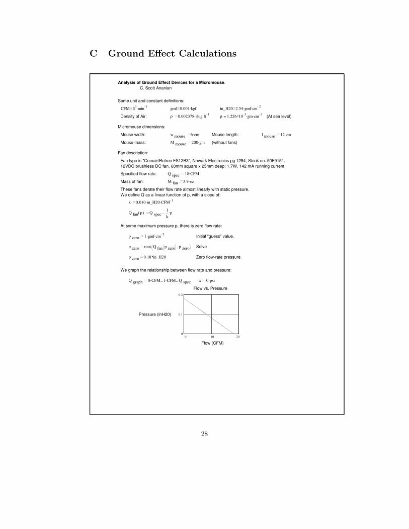
C Ground Effect Calculations

Analysis of Ground Effect Devices for a Micromouse. C. Scott Ananian

Some unit and constant definitions:

CFM .ft3 min 1 gmf .0.001 kgf in_H20 ..2.54 gmf cm 2

Density of Air: ρ ..0.002378 slug ft 3 =ρ 1.226 ..10 3 gm cm 3 (At sea level)

Micromouse dimensions:

Mouse width: w mouse.6 cm Mouse length: l mouse

.12 cm

Mouse mass: M mouse.200 gm (without fans)

Fan description:

Fan type is "Comair/Rotron FS12B3", Newark Electronics pg 1284, Stock no. 50F9151. 12VDC brushless DC fan, 60mm square x 25mm deep; 1.7W, 142 mA running current.

Specified flow rate: Q spec.18 CFM

Mass of fan: M fan.3.9 oz

These fans derate their flow rate almost linearly with static pressure. We define Q as a linear function of p, with a slope of:

k ..0.010 in_H20 CFM 1

Q fan( )p Q spec.1

kp

At some maximum pressure p, there is zero flow rate:

p zero..1 gmf cm 2 Initial "guess" value.

p zero root ,Q fan p zero p zero Solve

=p zero 0.18 in_H20 Zero flow-rate pressure.

We graph the relationship between flow rate and pressure:

Q graph ..,.0 CFM ..1 CFM Q spec x .0 psi

0 10 200

0.1

0.2

0.183.4688e-016

root ,Q fan( )x Q graph x

in_H20

180 Q graphCFM

Flow vs. Pressure

Pressure (inH20)

Flow (CFM)

28

Since power is defined as the product of pressure and flow rate, there is the following relation of power to flow rate:

0

0.05

0.1

0.0952211

0

.Q graph root ,Q fan( )x Q graph x

watt

180 Q graphCFM

Flow vs. Power

Power (Watts)

Flow (CFM)

Air cushion system.

Now we define the parameters of the air-cushion system. The mouse is in the shape of an ellipse, and the cushion wall is the outside edge of the mouse.

Number of fans: n 1

Cushion Perimeter: l cu.π .1

2w mouse

2 l mouse2 =l cu 29.804 cm

Effective Cushion Area: A c..π w mouse l mouse

Clearance height: h c.1 mm Discharge coefficient: D c 0.6

The fans pump air out from underneath the mouse to form a low-pressure area, generating a downward force to aid traction. Under steady-state conditions for this negative ground-effect vehicle, the air being pumped out of the space beneath the mouse is just sufficient to counteract the air leaking in through the gap beneath the chamber skirt. The force generated is obviously:

F cu p cu.p cu A c

Assuming that the air inside the chamber is initially at rest, the velocity of air escaping under the periperal gap is given by:

V c p cu

.2 p cu

ρ

The total volume flow of air into the chamber is thus:

Q gap p cu...h c l cu D c V c p cu

We solve for the steady state case where flow in equals flow out of the chamber:

p cu p zero Initial "guess" value.

Given

.n Q fan p cu...h c l cu D c

.2 p cu

ρ

p cu Find p cu

The steady-state pressure and corresponding fan flow rate is:=p cu 0.15 in_H20 =Q fan p cu 2.962 CFM

For comparison, the maximum (zero-flow rate) pressure specified for the fan is:=p zero 0.18 in_H20

29

Using the formula previously derived for generated force, we obtain:

F cu.p cu A c

=F cu 86.396 gmf Force generated by air cushion system

The augmentation factor is a measure of the effectiveness of air cushion as lift generating device:

K aA c

...2 h c l cu D c=K a 63.246

Now we analyze the weight/acceleration penalties of adding the ground effect device.

M ge M mouse.n M fan Mouse mass with ground effect fans

=F cu

.M ge g0.278 Added acceleration (in g's) due to ground effect fan.

For a "typical" one cell run in a maze (no maximum velocity restrictions), we might observe the following time improvement:

a before.0.5 g Best case for MITEE mouse III

a after a beforeF cu

M ge=a after 0.778 g

t .0 sec

t before.2 root ,..1

2a before t2 .9 cm t =t before 0.383 sec

t after.2 root ,..1

2a after t2 .9 cm t =t after 0.307 sec

=t before t after

t before19.843 %

In conclusion, this analysis indicates an almost 20% speed improvement using the ground effect devices.

References: J. Y. Wong, "Introduction to Air-cushion vehicles," in Theory of Ground Vehicles.

30

D Mechanical Drawings

D.1 Mouse front view

31

D.2 Mouse top view

32

D.3 Mouse bottom view

33

D.4 Gear train

D.5 Long-range sensor mount

34

EH

ardw

are

Schem

atic

s

E.1

Processo

rin

terfa

ce

4 3 2 1

A

B

C

D

1234

D

C

B

A

Date: April 11, 1997 Sheet 1 of 4

Size Document Number REV

C 1

TitleMicroMouse controller electronics

Princeton, NJ 08544Princeton UniversityC. Scott Ananian and Greg Humphreys

Ariadne Systems

VCCSDOUTSDINispENPLUGMODEGNDSCLK

12345678

J5

isp CONN.HDR1R.1/8

QUADA_LQUADB_LQUADA_RQUADB_R

ISP_SDOISP_SDI

ISP_MOD

ISP_CLK

GO_BUTTONSTOP_BUTTON

VCC VCC

13579

246810

J1

BDM conn.HDR2R.1/10

123456

J21

UNUSEDHDR2R.1/6

1 2 3 4 6 7 8 9

510

RP2

10k networkEXB-A

/BERRDSCLKFREEZEDSIDSO

UNUSED1

Background Debugging

Unused

/DS

/RESET

/BERR/HALT/DSACK0/DSACK1

TSCR/W

DSCLKMODCLK

VCC

VCC

1 2 3 4 6 7 8 9

510

RP1

10k networkEXB-A

DATA8DATA9DATA10DATA11DATA12DATA13DATA14DATA15A20 4

A19 5

A18 6

A17 7

A16 8

A15 10

A14 11

A13 12

A12 13

A11 17

A10 18

A9 19

A8 20

A7 22

A6 23

A5 24

A4 25

A3 26

A2 27

A1 28

A0 32

DQ15 52

DQ14 50

DQ13 47

DQ12 45

DQ11 41

DQ10 39

DQ9 36

DQ8 34

DQ7 51

DQ6 49

DQ5 46

DQ4 44

DQ3 40

DQ2 38

DQ1 35

DQ0 33

BYTE 31

CE0 14

CE1 2

OE 54

WE 55

WP 56

RP 16

RY/BY 53

3/5 1

VPP

15

U2LH28F016SUTTSOP-56

ADDR12ADDR13ADDR14ADDR15ADDR16ADDR17ADDR18ADDR19ADDR20

VCC

ADDR1ADDR2ADDR3ADDR4ADDR5ADDR6ADDR7ADDR8ADDR9ADDR10ADDR11

/OE

/CSBOOT

LED1POWER

GW_LED

LED2RUN

GW_LED

LED3ERROR

GW_LED

R68680RC0805A

R70680RC0805A

R69680

RC0805ADATA0DATA1DATA2DATA3DATA4DATA5DATA6DATA7

RY/BY

VCC

VCC

4.5mA current

TPUCH0 16TPUCH1 15TPUCH2 14TPUCH3 13TPUCH4 12TPUCH5 11TPUCH6 10TPUCH7 9TPUCH8 6TPUCH9 5TPUCH10 4TPUCH11 3TPUCH12 132TPUCH13 131TPUCH14 130TPUCH15 129

T2CLK 128PC7/ADDR23/CS10125

PC6/ADDR22/CS9124

PC5/ADDR21/CS8123

PC4/ADDR20/CS7122

PC3/ADDR19/CS6121

PC2/FC2/CS5120

PC1/FC1/CS4119

PC0/FC0/CS3118

/BGACK/CS2115

/BG/CS1114

/BR/CS0113

/CSBOOT112

ADDR18 42

ADDR17 41

ADDR16 38

ADDR15 37

ADDR14 36

ADDR13 35

ADDR12 33

ADDR11 32

ADDR10 31

ADDR9 30

ADDR8 27

ADDR7 26

ADDR6 25

ADDR5 24

ADDR4 23

ADDR3 22

ADDR2 21

ADDR1 20

ADDR0 90

DATA15 91

DATA14 92

DATA13 93

DATA12 94

DATA11 97

DATA10 98

DATA9 99

DATA8100

DATA7102

DATA6103

DATA5104

DATA4105

DATA3108

DATA2109

DATA1110

DATA0111

AN6/PADA6 53

AN5/PADA5 52

AN4/PADA4 49

AN3/PADA3 48

AN2/PADA2 47

AN1/PADA1 46

AN0/PADA0 45

VRH 50

VRL 51

/BKPT/DSCLK 56

/IFETCH/DSI 55

/IPIPE/DSO 54

FREEZE/QUOT 58

XFC 64

VDDSYN 61

TSC 57

R/W 79

/RESET 68

/HALT 69

/BERR 70

PF7/IRQ7 71

PF6/IRQ6 72

PF5/IRQ5 73

PF4/IRQ4 74

PF3/IRQ3 75

PF2/IRQ2 76

PF1/IRQ1 77

PF0/MODCLK 78

CLKOUT 66

XTAL 60

EXTAL 62PE7/SIZ1 80

PE6/SIZ0 81

PE5/AS 82

PE4/DS 85

PE3/RMC 86

PE2/AVEC 87

PE1/DSACK1 88

PE0/DSACK0 89

VSTBY 19

U1

MC68334GCFC20PQFP-132

ADDR19ADDR20

ECLKUNUSED1UNUSED2 UART_TX

UART_RX

F/R_LBRA_RBRA_L

WATCHDOG

UNUSED2UNUSED3UNUSED4UNUSED5UNUSED6

UNUSED5

UNUSED6

Quadrature Decode

1234

J4

Serial I/OHDR1R.1/4

R5 680 RC0805A

1234

J2

Left EncoderHDR1R.1/4

QUADA_L

VCC

VCC

Battery Monitor

R72110kRC0805A

R71110kRC0805A

VMtap

VM+

R4 680 RC0805A

1234

J3

Right EncoderHDR1R.1/4

QUADB_L

QUADA_RQUADB_R

VCC

ENA_RENA_LVEL_RVEL_L

QUADA_RQUADB_R

QUADA_LQUADB_L

F/R_R

AN0AN1AN2AN3TEMP

VSENSEHVSENSEL

ADDR6ADDR7ADDR8ADDR9ADDR10ADDR11ADDR12ADDR13ADDR14ADDR15ADDR16ADDR17ADDR18

/CSBOOT/CS0/CS1

DATA0DATA1DATA2DATA3DATA4DATA5DATA6

ADDRESS_BUS

A0 12

A1 11

A2 10

A3 9

A4 8

A5 7

A6 6

A7 5

A8 27

A9 26

A10 23

A11 25

A12 4

A13 28

A14 3

A15 31

A16 2

A17 30

A18 1

I/O0 13

I/O1 14

I/O2 15

I/O3 17

I/O4 18

I/O5 19

I/O6 20

I/O7 21

CE 22

WE 29

OE 24

U3

HM628512LTT-7SLTSOPII-32

ADDR1ADDR2ADDR3ADDR4ADDR5ADDR6ADDR7

/WE

A0 12

A1 11

A2 10

A3 9

A4 8

A5 7

A6 6

A7 5

A8 27

A9 26

A10 23

A11 25

A12 4

A13 28

A14 3

A15 31

A16 2

A17 30

A18 1

I/O0 13

I/O1 14

I/O2 15

I/O3 17

I/O4 18

I/O5 19

I/O6 20

I/O7 21

CE 22

WE 29

OE 24

U4

HM628512LTT-7SLTSOPII-32

ADDR8ADDR9ADDR10ADDR11ADDR12ADDR13ADDR14ADDR15ADDR16ADDR17ADDR18ADDR19

DATA_BUS

DATA7

/OE

/WE

/CS0

DATA6DATA7DATA8DATA9DATA10DATA11DATA12DATA13DATA14DATA15

ADDR0ADDR1ADDR2ADDR3ADDR4ADDR5

R6820RC0805A

/BERR

DSIDSO

DSCLK

R/W

/HALT

VRHVRL

GO_BUTTONSTOP_BUTTON

VCC

/RESET

Pull-ups in RP2

R7310kRC0805A

R7410kRC0805A

MGND

200mA max

SW2GO

SMT_SW

SW3STOP

SMT_SW

12

J6

FANHDR1R.1/2Q1

MOSFET NSOT-23(DSG2)

VM+

C5.1uFEIA_A

C2 22pFCC0805A

C1 22pF CC0805A

C40.1uF

CC1206A

R2 330kRC0805A

Y131.250kHz MC-405R1

10MRES200

FREEZE

MODCLK

TSC

RY/BYHOLD

FAN_ENSHS_LED

CLK_EN

/DS

DATA0DATA1DATA2DATA3DATA4DATA5

/DSACK0/DSACK1

AD_A0AD_A1AD_A2

UNUSED3UNUSED4

DATA8DATA9DATA10DATA11DATA12DATA13DATA14DATA15

/WE

/OE

/CS1

ADDR1ADDR2ADDR3ADDR4ADDR5ADDR6ADDR7ADDR8ADDR9ADDR10ADDR11ADDR12ADDR13ADDR14ADDR15ADDR16ADDR17ADDR18ADDR19

I1/CLK 2

I2 3

I3 4

I4 5

I5 6

I6 7

I7 9

I8 10

I9 11

I10 12

I/O1 27

I/O2 26

I/O3 25

I/O4 24

I/O5 23

I/O6 21

I/O7 20

I/O8 19

SDO 22

SDI 15

MODE 8

SCLK 1

I11 13

I12 16

I/O9 18

I/O10 17

U6

ISPGAL22V10C-7LJPLCC28

R/W/DS

/RESETQBQC

DATA0DATA1DATA4

DATA11DSCLK

/OE/WE

DATA9

CLKRST

ANALOG_MULTI_ADDRESSC3.1uFEIA_A

R3

470RC0805A

VCC

C60.01uFCC0805A

CLK_ENCLK_200k I1/CLK 2

I2 3

I3 4

I4 5

I5 6

I6 7

I7 9

I8 10

I9 11

I10 12

I/O1 27

I/O2 26

I/O3 25

I/O4 24

I/O5 23

I/O6 21

I/O7 20

I/O8 19

SDO 22

SDI 15

MODE 8

SCLK 1

I11 13

I12 16

I/O9 18

I/O10 17

U16


CLK_10kDCLK_10k

MGND

200mA max

Q9MOSFET N

SOT-23(DSG2)

12

J16

LASERHDR1R.1/2

Q10MOSFET N

SOT-23(DSG2)

12

J17

LASERHDR1R.1/2

12

J22

LASER_POWERHDR1R.1/2

VCC

ISP_SDOISP_SD3ISP_MODISP_CLK

Motor Drivers

MOTOR.SCH

F/R_RENA_RBRA_RVEL_R

F/R_LENA_LBRA_LVEL_L

ISP_SD3ISP_SD1ISP_MODISP_CLK



Analog Interface

ANALOG.SCH

AD_A2AD_A1AD_A0

HOLD

AN0AN1AN2AN3

CLK_200k

SHS_LEDVRH

DCLK_10k

AD_A0AD_A1AD_A2

HOLD

AN0AN1AN2AN3

CLK_200k

SHS_LEDVRH

DCLK_10k

Power Supply

POWER.SCH

VRHVRL

TEMP

VMtapVMtap

VRHVRL

TEMP

ECLK

CLKRST

VCC

A 14

B 1

R0(1) 2

R0(2) 3

QA 12

QB 9

QC 8

QD 11

U7

SN74LS93DSO14

ISP_SD1ISP_SDIISP_MODISP_CLK

QBQC

CLK_200k

VCC 1

VCC 2 RESET 7

WDI 6

GND 8 GND 4 GND 3

U5

LTC699IS8SO8

VCC

SW1

MANUAL RESETSMT_SW

WATCHDOGISP_CLKISP_MOD

ISP_SD3ISP_SD1

35

E.2

Analo

gele

ctr

onic

s

4 3 2 1

A

B

C

D

1234

D

C

B

A



C


Princeton University

3

2 1

U14A

OP490GSSOL16

R771.0kRC0805AR76 9.1k

RC0805A

ANALOG_MULTI_ADDRESS

AGND

3rd order Butterworth Low-PassCenter Freq. 1kHz

C12.022uFCC1206A

C11.056uFCC1210A

C13.0033uFCC0805A

R3110k

RC0805A

R3310k

RC0805A

R3210k

RC0805A

10kHz*20

SynchronousDemodulator

R55 10kRC0805A

R56 4.99k

RC0805A

R1510k

RC0805A

3

2 1

U13A

OP490GSSOL16

VDD

AGND

VEE

Switched CapacitorBandpass Filter

R14 100kRC0805A

R12

10kRC0805A

R1310k

RC0805A

INV 12

HP/N 11

BP 10

LP 9

S 8

CLK 18

V+ 7

AGND 6

V- 19

U11A

LTC1264CSWSOL24

Gain SetPreamp

1234

J7

LRS1HDR1R.1/4

R11

1MRC0805A

3

2 1

U12A

OP490GSSOL16

AGND

Gain SetPreamp

R16

1MRC0805A

5

6 7

U12B

OP490GSSOL16AGND


C72700pFCC1206A

R19 100kRC0805A

R17

10kRC0805A

R1810k

RC0805A

INV 1

HP/N 2

BP 3

LP 4

S 5

CLK 18

V+ 7

AGND 6

V- 19

U11B

LTC1264CSWSOL24

10kHz*20


Q2MOSFET NSOT-23(DSG2)

R57 10kRC0805A

R58 4.99k

RC0805A

R2010k

RC0805A

5

6 7

U13B

OP490GSSOL16

VDD

AGND

AGND

VEE


C15.022uFCC1206A

C14.056uFCC1210A

C16.0033uFCC0805A

R3410k

RC0805A

R3610k

RC0805A

R3510k

RC0805A

AGND AGND

5

6 7

U14B

OP490GSSOL16

S1 4

S2 5

S3 6

S4 7

S5 12

S6 11

S7 10

S8 9

D 8

A0 1A1 16A2 15

EN 2

U9

ADG408BRSO16

R791.0kRC0805AR78 9.1k

RC0805A

SHST1SHST2SHST3SHST4SHST5SHST6

AGND

R10 30kRC0805A

R810k

RC0805A

3

2 1

U15A

OP285GSSO8

AD_A0AD_A1AD_A2

VCC VIN1 3

S/H1 6

VIN2 5

S/H2 7

VIN3 11

S/H3 9

VIN4 12

S/H4 10

VOUT1 2

VOUT2 1

VOUT3 15

VOUT4 14

U8

SMP04ESSO16

HOLD

AN0

AN1

AN2

AN3

R9 30kRC0805A

5

6 7

U15B

OP285GSSO8

AD_A0AD_A1AD_A2

VCC

AGND

S1 4

S2 5

S3 6

S4 7

S5 12

S6 11

S7 10

S8 9

D 8

A0 1A1 16A2 15

EN 2

U10

ADG408BRSO16

R811.0kRC0805AR80 9.1k

RC0805A

SHSB1SHSB2SHSB3SHSB4SHSB5SHSB6

AGND


C17.056uFCC1210A

AGND AGND

10kHz*20



R2510k

RC0805A

AGND


C82700pFCC1206A

R22

10kRC0805A

R2310k

RC0805A

INV 24

HP/N 23

BP 22

LP 21

S 20

CLK 18

V+ 7

AGND 6

V- 19

U11C

LTC1264CSWSOL24

Gain SetPreamp

R21

1MRC0805A

Gain SetPreamp

1234

J8

LRS2HDR1R.1/4

R26

1MRC0805A

10

9 8

U12C

OP490GSSOL16

AGND


C92700pFCC1206A

R24 100kRC0805A

R27

10kRC0805A

R2810k

RC0805A

INV 13

HP/N 14

BP 15

LP 16

S 17

CLK 18

V+ 7

AGND 6

V- 19

U11D

LTC1264CSWSOL24

10kHz*20



R59 10kRC0805A

R60 4.99k

RC0805A

R3010k

RC0805A

10

9 8

U13C

OP490GSSOL16

VDD

AGND

VEE

AGND 3rd order Butterworth Low-PassCenter Freq. 1kHz

C18.022uFCC1206A

C19.0033uFCC0805A

R3710k

RC0805A

R3910k

RC0805A

R3810k

RC0805A

AGND AGND

10

9 8

U14C

OP490GSSOL16

R831.0kRC0805AR82 9.1k

RC0805A

R710k

RC0805A

AGND

DCLK_10kCLK_200k

12

1314

U14D

OP490GSSOL16

AGND

C21.022uFCC1206A

C20.056uFCC1210A

C22.0033uFCC0805A

R4010k

RC0805A

R4210k

RC0805A

R4110k

RC0805A

AGND AGND


R61 10kRC0805A

R62 4.99k

RC0805A

12

1314

U13D

OP490GSSOL16

VDD

AGND

VEE

AGND

C102700pFCC1206A

R29 100kRC0805A 12

1314

U12D

OP490GSSOL16

VRH

AGND

LEDTOPBOTGND

LEDTOPBOT

VCC

VCC

12345

J9SHS1

HDR1R.1/5

12345

J10SHS2

HDR1R.1/5

1

16

R44A220k

EXB-V16

1

16

R43A20k

EXB-V16

2

15

R44B220k

EXB-V16

2

15

R43B20k

EXB-V16

SHST1

SHST2

SHSB1

SHSB2

VCC

VCCAGND

3

14

R44C220k

EXB-V16

3

14

R43C20k

EXB-V16

4

13

R44D220k

EXB-V16

4

13

R43D20k

EXB-V16

5

12

R43E20k

EXB-V16

5

12

R44E220k

EXB-V16

6

11

R44F220k

EXB-V16

6

11

R43F20k

EXB-V16 1 2 3 4 6 7 8 9

5 10

RP3100 networkEXB-A

AD_A2

AD_A0AD_A1

AN0AN1AN2AN3

HOLD

CLK_200k

AD_A0AD_A1AD_A2

HOLD

AN0AN1AN2AN3

CLK_200k

SHS_LEDVRH

DCLK_10kSHS_LED

VRH

DCLK_10k

Q6 MOSFET NSOT-23(DSG2)SHS_LED

GND

LEDTOPBOTGND

LEDTOPBOT

VCC

VCC

12345

J11SHS3

HDR1R.1/5

12345

J12SHS4

HDR1R.1/5

SHST3

SHST4

SHSB3

SHSB4

VCC

VCC

AGND

AGND

GND

LEDTOPBOTGND

LEDTOPBOTGND

VCC

VCC

12345

J13SHS5

HDR1R.1/5

12345

J14SHS6

HDR1R.1/5

SHST5

SHST6

SHSB5

SHSB6

VCC

VCC

AGND

AGND

AGND

36

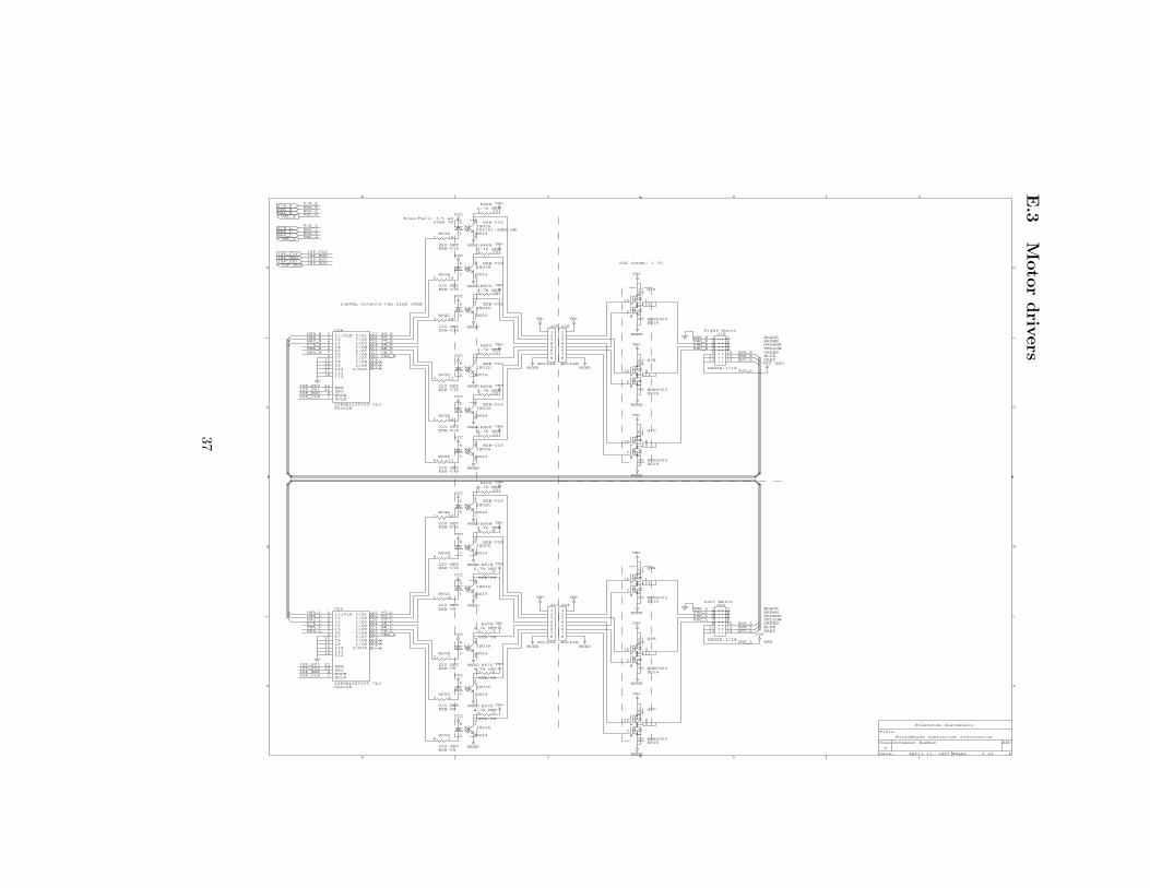
E.3

Moto

rdriv

ers

4 3 2 1

A

B

C

D

1234

D

C

B

A



C



VGS thres. 1-3V

2 15

R66B4.7k NET

EXB-V16

2

1

16

15

ISO1APS2701-4NEC-NDSO16

4

3

14

13

ISO1B

SO16

1 16

R66A4.7k NET

EXB-V16

VCC

VM+

VCC

VM+MGND

50mA IfRise/Fall: 3/5 uS

1 16R64A

220 NETEXB-V16



ISP_CLKISP_MODISP_SD1ISP_SD3



ISP_CLKISP_MODISP_SD1ISP_SD3

ispGAL outputs can sink 16mA

I1/CLK 2

I2 3

I3 4

I4 5

I5 6

I6 7

I7 9

I8 10

I9 11

I10 12

I/O1 27

I/O2 26

I/O3 25

I/O4 24

I/O5 23

I/O6 21

I/O7 20

I/O8 19

SDO 22

SDI 15

MODE 8

SCLK 1

I11 13

I12 16

I/O9 18

I/O10 17

U24


HSA_R

2 15R64B

220 NETEXB-V16

3 14R64C

220 NETEXB-V16

AT_R

3 14

R66C4.7k NET

EXB-V166

5

12

11

ISO1C

SO16

VCC

VM+

VM+

MGND

MGND

15

2

116

14

11

63

Q7A

NDM3000SO16

12345678

J25

MotorA

12345678

J26

MotorB

VM+

VM+

MGND+ 1

+ 3

+ 5

+ 7

+ 9

+ 11

+ 13

+ 2

+ 4

+ 6

+ 8

+ 10

+ 12

+ 14

J19Right Motor

HDR2R.1/14

BROWNORANGEYELLOW

RED

BLACK

GREENBLUEGREY

HSA_RHSB_RHSC_R

VDD_R

VCC

PHA_RPHB_RPHC_R

GND_R

12

5

413

14

11

63

Q7B

NDM3000SO16

VM+

MGND

MGND

4 13

R66D4.7k NET

EXB-V16

5 12

R66E4.7k NET

EXB-V16

8

7

10

9

ISO1D

SO16

2

1

16

15

ISO2A

SO16

VCC

VM+

VCC

VM+MGND

MGND

4 13R64D

220 NETEXB-V16

BT_RCT_RAB_RBB_RCB_RVEL_R

HSB_RHSC_RF/R_RENA_RBRA_R


5 12R64E

220 NETEXB-V16

6 11R64F

220 NETEXB-V16

6 11

R66F4.7k NET

EXB-V164

3

14

13

ISO2B

SO16

VCC

VM+MGND

MGND

10

7

89

14

11

63

Q7C

NDM3000SO16

VM+

MGND

7 10

R66G4.7k NET

EXB-V16

8 9

R66H4.7k NET

EXB-V16

6

5

12

11

ISO2C

SO16

8

7

10

9

ISO2D

SO16

VCC

VM+

VCC

VM+MGND

7 10R64G

220 NETEXB-V16

I1/CLK 2

I2 3

I3 4

I4 5

I5 6

I6 7

I7 9

I8 10

I9 11

I10 12

I/O1 27

I/O2 26

I/O3 25

I/O4 24

I/O5 23

I/O6 21

I/O7 20

I/O8 19

SDO 22

SDI 15

MODE 8

SCLK 1

I11 13

I12 16

I/O9 18

I/O10 17

U25


HSA_L

8 9R64H

220 NETEXB-V16

1 8R65A

220 NETEXB-V8

AT_L

1 8

R67A4.7k NET

EXB-V82

1

16

15

ISO3A

SO16

VCC

VM+

VM+

MGND

MGND

15

2

116

14

11

63

Q8A

NDM3000SO16

12345678

J23

MotorA

12345678

J24

MotorB

VM+

VM+

MGND+ 1

+ 3

+ 5

+ 7

+ 9

+ 11

+ 13

+ 2

+ 4

+ 6

+ 8

+ 10

+ 12

+ 14

J20Left Motor

HDR2R.1/14

PHA_LGND_L

BROWNBLACK

ORANGEYELLOW

RED

GREENBLUEGREY

HSA_LHSB_LHSC_L

VDD_L

VCC

PHB_LPHC_L

12

5

413

14

11

63

Q8B

NDM3000SO16

VM+

MGND

MGND

2 7

R67B4.7k NET

EXB-V8

3 6

R67C4.7k NET

EXB-V8

4

3

14

13

ISO3B

SO16

VCC

VM+

VCC

VM+MGND

MGND

2 7R65B

220 NETEXB-V8

BT_LCT_LAB_LBB_LCB_LVEL_L

HSB_LHSC_LF/R_LENA_LBRA_L


3 6R65C

220 NETEXB-V8

4 5R65D

220 NETEXB-V8

4 5

R67D4.7k NET

EXB-V8

6

5

12

11

ISO3C

SO16

8

7

10

9

ISO3D

SO16

VCC

VM+MGND

MGND

10

7

89

14

11

63

Q8C

NDM3000SO16

VM+

MGND

37

E.4

Pow

er

supply



B



Analog Board

Primary Digital Supply+5V @ 1A

VCC

Digital Board

IN 1 OUT 3

GND

2

U19LM2940CT-5.0

TO-220X

8V @ 1A

Intermediate Voltage

IN 1 OUT 3

GND

2

U26LM2940T-8.0

TO-220X

Power Board

8V @ 1A

C7522uFPANA_C

C3010uF

PANA_C

C2522uFPANA_C

INPUT 8

SHUTDOWN 3

GROUND 4

OUTPUT 1

SENSE 2

FEEDBACK 7

VTAP 6

ERROR 5

U20

LP2951ACMSO8

Analog Positive Supply+5V @ 100 mA

C2422uFPANA_C

VDDVoltage Reference

C3247uFEIA_D

VRHVRH

C33.1uFEIA_A

C311uFEIA_A

+VIN

2

NC

7

NC 1

TEMP 3

GND

4

SEL

8

VOUT 6

TRIM 5

U22

AD780ARSO8

C2822uF

PANA_C TEMP TEMPAGND

IN 2 OUT 3

GND

1

U21LM2990S-5.0TO-263-3

C2910uFPANA_C

R63

0 RC1206

LV 6OSC 7

CAP+ 2

CAP- 4

VOUT 5V+ 8

GND 3

U18

ICL7660SCBASO8

C2622uF

PANA_CD1

DO-214C27100uFCAP200PX

IN 1 OUT 3

GND

2

U17LM2940T-8.0

TO-220X

VMtap

VM+

Motor Power Supply

+12

J15

Left BatteryBATTCONN

VMtap

+12

J18

Right BatteryBATTCONN

R75

0RC1206 VSS

MGND

C2310uFPANA_C

C7622uFPANA_C

IN 1 OUT 3

GND

2

U27LM2940CT-5.0

TO-220X

Secondary Digital Supply+5V @ 0.5 A

VCC2Analog Negative Supply-5V @ 100 mA

VEE

IN 1 OUT 3GND

2

U23LP2950ACZ-3.3

TO-92

VDD

VRLVRL

VRH

VRL

VDD

AGNDADG608 Safety

VDD

SMP04ES

Digital Board

VDD68334

Bypass CapacitorsVCC

C34.1uFEIA_A

C35.1uFEIA_A

C36.1uFEIA_A

C37.1uFEIA_A

C38.1uFEIA_A

C39.1uFEIA_A

C40.1uFEIA_A

C41.1uFEIA_A

C42.1uFEIA_A

Safety

C43.1uFEIA_A

C44.1uFEIA_A

C45.1uFEIA_A

C46.1uFEIA_A

C56.1uFEIA_A

C55.1uFEIA_A

VEE

AGNDC60.1uFEIA_A

C59.1uFEIA_A

C58.1uFEIA_A

C57.1uFEIA_A

VEE

AGND AGND

C731uFEIA_A

C741uFEIA_A

VEE

C69.1uFEIA_A

C70.1uFEIA_A

OP490

C63.1uFEIA_A

C64.1uFEIA_A

C65.1uFEIA_A

C66.1uFEIA_A

C67.1uFEIA_A

C68.1uFEIA_A

VDD

AGND

LTC1264

C61.1uFEIA_A

C62.1uFEIA_A

VDD

VCC

AGND

C711uFEIA_A

C721uFEIA_A

VCC74LS93

C52.1uFEIA_A

C53.1uFEIA_A

C54.1uFEIA_A

VCC628512 ispGAL22V10

C49.1uFEIA_A

C50.1uFEIA_A

C51.1uFEIA_A

VCC2

28F016

628512

C47.1uFEIA_A

C48.1uFEIA_A

VCC

VEE VEE

38

theseus: a maze-solving robot c. scott ananian and greg

Documents