thermodynamics, maximum power, and the dynamics of
TRANSCRIPT
Hydrol. Earth Syst. Sci., 17, 225–251, 2013www.hydrol-earth-syst-sci.net/17/225/2013/doi:10.5194/hess-17-225-2013© Author(s) 2013. CC Attribution 3.0 License.
Hydrology and
Earth System
Sciences
Thermodynamics, maximum power, and the dynamics ofpreferential river flow structures at the continental scaleA. Kleidon1, E. Zehe2, U. Ehret2, and U. Scherer21Max-Planck Institute for Biogeochemistry, Hans-Knoll-Str. 10, 07745 Jena, Germany2Institute of Water Resources and River Basin Management, Karlsruhe Institute of Technology – KIT, Karlsruhe, Germany
Correspondence to: A. Kleidon ([email protected])
Received: 14 May 2012 – Published in Hydrol. Earth Syst. Sci. Discuss.: 11 June 2012Revised: 14 December 2012 – Accepted: 22 December 2012 – Published: 22 January 2013
Abstract. The organization of drainage basins shows somereproducible phenomena, as exemplified by self-similar frac-tal river network structures and typical scaling laws, andthese have been related to energetic optimization principles,such as minimization of stream power, minimum energy ex-penditure or maximum “access”. Here we describe the or-ganization and dynamics of drainage systems using thermo-dynamics, focusing on the generation, dissipation and trans-fer of free energy associated with river flow and sedimenttransport. We argue that the organization of drainage basinsreflects the fundamental tendency of natural systems to de-plete driving gradients as fast as possible through the maxi-mization of free energy generation, thereby accelerating thedynamics of the system. This effectively results in the maxi-mization of sediment export to deplete topographic gradientsas fast as possible and potentially involves large-scale feed-backs to continental uplift. We illustrate this thermodynamicdescription with a set of three highly simplified models re-lated to water and sediment flow and describe the mecha-nisms and feedbacks involved in the evolution and dynam-ics of the associated structures. We close by discussing howthis thermodynamic perspective is consistent with previousapproaches and the implications that such a thermodynamicdescription has for the understanding and prediction of sub-grid scale organization of drainage systems and preferentialflow structures in general.
1 Introduction
River networks are a prime example of organized structuresin nature. The effective rainfall, or runoff, from land does
not randomly diffuse through the soil to the ocean, but rathercollects in channels that are organized in tree-like structuresalong topographic gradients. This organization of surfacerunoff into tree-like structures of river networks is not a pe-culiar exception, but is persistent and can generally be foundin many different regions of the Earth. Hence, it would seemthat the evolution and maintenance of these structures of rivernetworks is a reproducible phenomenon that would be the ex-pected outcome of how natural systems organize their flows.The aim of this paper is to understand the basis for whydrainage systems organize in this way and relate this to thefundamental thermodynamic trend in nature to dissipate gra-dients as fast as possible. Such a basis will likely help us tobetter understand the central question of hydrology regardingthe partitioning of precipitation into evaporation and runofffrom first principles.
1.1 River systems and organizational principles
Several approaches have tried to understand this form of or-ganization from basic organization principles that involvedifferent forms of energetic optimization (see, e.g. the re-view by Phillips, 2010 and Paik and Kumar, 2010) or fromstability analysis of the conservation of sediment and waterand transport laws (e.g. Kirkby, 1971; Smith and Bretherton,1972). While the latter studies also provide explanations forthe evolution of spatial structures in river basins, these stud-ies do not consider changes in energy specifically. We focushere on those studies that deal with principles that explicitlytreat conversions of energy, as these are most closely relatedto thermodynamics and the second law, and thus should havethe greatest potential for formulating organizational princi-ples in the most general terms.
Published by Copernicus Publications on behalf of the European Geosciences Union.

226 A. Kleidon et al.: Thermodynamics and maximum power of river systems
In terms of energetic principles, Woldenberg (1969)showed that basic scaling relationships of river basins canbe derived from optimality assumptions regarding streampower. Similarly, Howard (1990) described optimal drainagenetworks from the perspectives that these minimize the to-tal stream power, while Rodriguez-Iturbe et al. (1992a,b)and Rinaldo et al. (1992) used the assumption of “minimumenergy expenditure” (also Leopold and Langbein, 1962;Rodriguez-Iturbe and Rinaldo, 1997) and were able to repro-duce the observed, fractal characteristics of river networks.Similar arguments were made by Bejan (1997) in the con-text of a “constructal law”, which states that the evolution ofriver networks should follow the trend to maximize “access”(the meaning of “access”, however, is ambiguous and diffi-cult to quantify). Likewise, West et al. (1997) showed thatthe assumption of minimizing frictional dissipation in threedimensional networks yields scaling characteristics in treesand living organisms that are consistent with observations.Related to these energetic minimization principles are
principles that seem to state exactly the opposite: that sys-tems organize to maximize power, dissipation or, more gen-erally, entropy production. These three aspects are closelyrelated. While power, the rate at which work is performedthrough time, describes the generation of free energy, thisfree energy is dissipated into heat in a steady state, resultingin entropy production. This maximization is also related tominimization. When frictional dissipation of a moving fluidis minimized, its ability to transport matter along a gradi-ent is maximized. This aspect is further explored in moredetail in this manuscript for the case of river networks aswell as their surrounding hillslopes. Hence, the maximiza-tion of any of these aspects in steady state yields roughlythe same result, namely, that driving gradients that yield thepower to drive the dynamics are dissipated as fast as pos-sible. The maximum power principle was originally formu-lated in electrical engineering in the 19th century, and foundrepeated considerations in biology (Lotka, 1922a,b), ecology(Odum, 1969, 1988) and Earth system science (e.g. Klei-don, 2010a). Closely related but developed independently,the proposed principle of Maximum Entropy Production(MEP) was first formulated in atmospheric sciences by Pal-tridge (1975, 1979) and has recently gained attention, e.g. inattempting to derive it theoretically from statistical physicsand information theory (Dewar, 2005, 2010), in applying itto a variety of environmental systems (Kleidon et al., 2010;Kleidon, 2010b) and to land surface hydrology in particular(e.g. Wang and Bras, 2011; Kleidon and Schymanski, 2008).A recent example of the application of maximum dissipa-tion to preferential water flow in soils is given in Zehe etal. (2010).In this paper, we use a thermodynamic perspective of the
whole continental system to show that these proposed opti-mality principles are not contrary to each other, but all re-flect the overall trend in Earth system functioning to depletedriving gradients as fast as possible. The term “as fast as
possible” is non-trivial and is fundamentally constrained bythe conservation laws of energy, mass, and momentum. Ap-plied to river network structures, this general trend translatesinto the hypothesis that these network structures form be-cause they represent the means to deplete the topographicgradients at the fastest possible rate. This might appear coun-terintuitive at first sight. It would seem that the second law ofthermodynamics would imply that gradients and thus spatialorganization are depleted, and not created. As we will seebelow, it is through a “detour” of structure formation thatthe overall dynamics to deplete gradients are accelerated andhence the presence of structure can be interpreted as the re-sult of the second law of thermodynamics in a broader sense.To evaluate this hypothesis, we need to understand the ener-getic limits to sediment transport, but we also need to take abroader view of what is driving continental dynamics and to-pographic gradients in the first place as these set the flexibleboundary conditions for river flow and its organization.
1.2 River systems in the broader, continental context
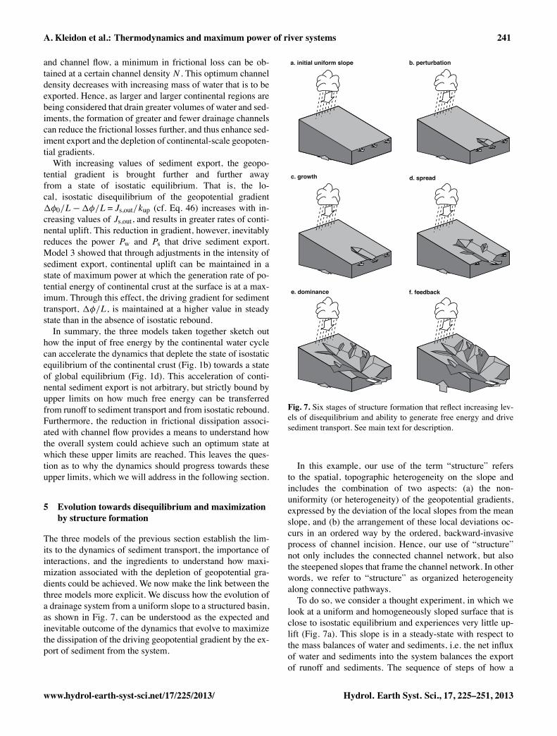
To understand the depletion of topographic gradients in rela-tion to changes in energy and the second law, we need to lookat the broader context of the processes that shape topographicgradients. This context involves the dynamics of the conti-nental crust as illustrated in Fig. 1 in a highly simplified way.This figure shows the dynamics of topographic gradients onland in terms of three steps from an initial state of local, iso-static equilibrium of continental crust to a state of global,“stratigraphic” equilibrium in which continental crust is uni-formly distributed over the planet. This trend from Fig. 1ato c is reflected in an energetic trend of decreased potentialenergy. In this idealized setup, we make the simplifying as-sumption that there is no tectonic activity that would act toform and concentrate continental crust and thus maintain thegeneration of continents.To relate the trend to energetic changes, we note that the
energy that describes the system consists of the potentialenergies of continental and oceanic crust. Continental crusthas a lower density than oceanic crust. At our starting point,Fig. 1a, the two masses are in a state of local, isostatic equi-librium. This state is associated with no uplift or subsidenceof continental crust, since the buoyancy force due to the dif-ference in densities is balanced by gravity. This local stateis associated with a horizontal gradient in topography, hererepresented by the difference�z =�zc,l− �zo,l, which mea-sures the tops of the two types of crust to a reference depth.The lowest value of potential energy in the system would
be achieved in a state of “global equilibrium”, in which thematerial of the continental crust is uniformly spread out overthe whole surface of the Earth, as shown in Fig. 1c. The as-sociated reduction in potential energy is shown mathemati-cally in the Appendix. In this state, the potential energy ofthe oceanic crust and the upper mantle would overall be low-ered to an elevation below �zo,g, while the potential energy
Hydrol. Earth Syst. Sci., 17, 225–251, 2013 www.hydrol-earth-syst-sci.net/17/225/2013/
A. Kleidon et al.: Thermodynamics and maximum power of river systems 227
a. local, isostatic equilibrium
Δzc,l
atmosphere
oceanic crust/mantle
continentalcrust
LLc
Δzo,l
b. local disequilibrium by sediment transport
atmosphere
oceanic crust/mantle
watercycle
LLc
continentalcrust
continentaluplift
sedimenttransport
c. global, stratigraphic equilibrium
atmosphere
oceanic crust/mantle
continentalcrust
L, Lc
Δzc,g
Δzo,g
Fig. 1. Highly simplified diagram to illustrate how continental crustevolves from (a) a state of local, isostatic equilibrium through (b) astate with sediment transport to (c) a state of global, stratigraphicequilibrium. Sediment transport provides the means to efficientlytransport continental crust along topographic gradients in the hor-izontal and thereby minimizes the potential energy within the sys-tem (see Appendix for details). The ocean is shown in black andplays a critical role here as the driver of the hydrologic cycle (thinarrows), which in turn provides a substantial power source to accel-erate sediment transport. Plate tectonics is excluded for simplicity.The symbols in the figures are used in the Appendix to quantify thisdirection towards minimizing the potential energy associated withoceanic and continental crust.
of the continental crust would be lowered to an elevation be-low �zc,g.The critical point relating to the role of river networks is
that getting from step (a) to (c) without fluvial transport ofsediments is extremely slow. With the work done by runoffand river flow in organized network structures on sedimenttransport, the depletion of the driving gradient�z is, overall,substantially enhanced, possibly to the fastest possible rateallowed by the system setting. Hence, our hypothesis relatesto step (b) shown in Fig. 1b. To evaluate this hypothesis, weneed to consider the response of continental uplift to the ero-sion of topographic gradients by sediment transport.
1.3 Structure of the paper
In the following, we first provide a brief overview of ther-modynamics to provide the context of a thermodynamic de-scription of the Earth system in Sect. 2. We then formulatedrainage systems as thermodynamic systems and describetheir dynamics in terms of conversions of energy of differ-ent forms. We then set up three simple models to demon-strate the means by which drainage basins act to maximizesediment transport and thereby the depletion of geopotentialgradients of continental crust. These examples are kept ex-tremely simple to show that such maximum states exist andwhat it needs to evolve to these maximum states. In Sect. 5we then explore why the evolution and dynamics of structureformation associated with river networks should be directedtowards achieving these maximum power states. In Sect. 6we characterize these dynamics in terms of different timescales that are based on rates of free energy generation andgradient depletion and the associated feedbacks that shapethe dynamics. In the discussion we then relate our results toprevious work on river networks, in particular to proposedenergy minimization principles, and more generally to ther-modynamics and optimality and explore the implications ofthese results. We close with a brief summary and conclusion.
2 Brief overview of the thermodynamics of Earthsystem processes
Thermodynamics is a fundamental theory of physics thatdeals with the general rules and limits for transforming en-ergy of different types. It is commonly applied to conversionsthat involve heat, and to systems with fixed boundary condi-tions, such as a heat engine. The scope of thermodynamics is,however, much wider. In the following overview, we sketchout the common basis to describe a system in terms of ex-changes of energy of different forms and how the first andsecond law of thermodynamics provide the limits of conver-sion rates from one form of energy into another. We thendescribe how thermodynamics provides the basis to describethe dynamics of systems in the context of Earth system func-tioning at large.
www.hydrol-earth-syst-sci.net/17/225/2013/ Hydrol. Earth Syst. Sci., 17, 225–251, 2013
228 A. Kleidon et al.: Thermodynamics and maximum power of river systems
Table 1. Different forms of energy relevant for the description of drainage basin dynamics and their thermodynamic description as pairs ofconjugate variables, one extensive variable that depends on the size of the system, and one intensive variable that is independent of the sizeof the system.
form of energy extensive intensive variable expression associated fluxesvariable variable for work and conservation laws
thermal entropy temperature dW = d(S T ) cpρ dT /dt =�JhS T (heat balance)
kinetic momentum velocity dW = d(pv) dp/dt =�F
p =mv v (momentum balance)
potential mass geopotential dW = d(mgz) dm/dt =�Jm(or gravitational) m (or gravitational (mass balance)
potential)g z
We start with the general description of a system in termsof its various contributions to the total energy U of the sys-tem. The different forms of energy can be described in termsof sets of conjugate variables, consisting each of an intensivevariable that is independent of the size of the system, suchas temperature, pressure, charge, surface tension or geopo-tential, and an extensive variable, which depends on the sizeof the system, such as entropy, volume, voltage, surface areaor mass. A brief overview of these sets of variables and therelated forms of energy relevant here is summarized in Ta-ble 1, while an overview of the thermodynamic terminologyis provided in Table 2.The formulation of the dynamics of a system in terms of
the conjugate variables and associated forms of energy setthe basis for applying the first and second law of thermo-dynamics to the dynamics. The first law of thermodynamicsessentially states the conservation of energy, i.e. it states thatthe sum of all changes of energy within the system balancesthe energy exchanges with the surroundings. Traditionally,the first law is expressed as the change in total energy dUof the system being balanced by external heating dQ and thework done by the system dW :
dU = dQ − dW. (1)
When we take a broader view of the total energy of thesystem, then dW is not removed from the system, but ratherconverted into another form of energy. For instance, when asmall amount of work dW is being performed from differen-tial heat to generate motion, kinetic energy is increased bydW at the expense of heat, which is reduced by −dW . Dur-ing this conversion process, the total energy of the systemremains constant, dU = 0, and it is merely the form of energythat is being altered. When we include these forms of en-ergy as contributions to the total energy of the system, thenthe first law limits the energy conversions within the system,and the dW term represents the conversion of heat to someother form of energy. More specifically, the dW term repre-sents the work done to create a gradient in another variable
under conservation of mass, momentum and other conserva-tion laws. For instance, when motion is generated (i.e. workis performed to accelerate mass), this corresponds to the gen-eration of a velocity gradient at the expense of exploiting an-other gradient (e.g. heating or geopotential). When work isperformed to lift mass, it corresponds to the generation ofa gradient in the geopotential, again, at the expense of ex-ploiting another gradient (e.g. a velocity gradient). Hence,the dynamics within the system is all about converting gra-dients associated with one form of energy into gradients ofanother form of energy. In a broader sense, the first law tellsus to do the proper accounting of the build-up and depletionof gradients of different types. These gradients allow workto be derived from them, so these gradients are associatedwith free energy, i.e. energy that is able to perform work.Note that sometimes this is referred to as “exergy”, or spe-cific forms of free energy are used (e.g. Gibbs free energy,Helmholtz free energy). In the following, we will refer to theterm “free energy” in a general way as a gradient in a vari-able associated with a certain form of energy that can be usedto generate another gradient. We will refer to the generationterm dW /dt =P as the power associated with this conversion.In this context, a broader interpretation of the first law tellsus that the total of all energy conversions between differentforms of energy within a system need to balance the energyexchanges with the surroundings.The second law of thermodynamics states that the entropy
of an isolated system can only increase. When this law is ex-tended to non-isolated systems that exchange energy and/ormass, it takes the form of a constraint for the budget of thesystem’s entropy S:
dS/dt = σ +�
i
Js,i , (2)
where σ ≥ 0 is the entropy produced within the system by ir-reversible processes, and
�i
Js,i is the sum of all entropy ex-
change fluxes with the surroundings associated with energy-and mass exchange. By constraining σ to values greater or
Hydrol. Earth Syst. Sci., 17, 225–251, 2013 www.hydrol-earth-syst-sci.net/17/225/2013/
A. Kleidon et al.: Thermodynamics and maximum power of river systems 229
Table 2. Overview of the different thermodynamic terms used here, their brief definitions and their relevance to hydrologic processes.
term description examples used here
conjugate variables A set of two variables for which the product describes a see Table 1form of energy. The pair is formed by one intensive andone extensive variable.
extensive variable a variable that depends on the size of the system stocks of water (soil, river, water vapor), momentum of flow
intensive variable a variable that does not depend on the size of the system geopotential (or gravitational potential), flow velocity
heat a specific form of energy measured by temperature soil heat storage(better term: thermal energy)
work the conversion of one form of energy into another; acceleration or lifting of water and sedimentmechanical definition: the exertion of a force over adistance
entropy unavailability of a system’s thermal energy for thermal energy is only considered in this manuscript asconversion into mechanical work. the end result of dissipative processes
free energy the capacity of a form of energy to perform work potential energy of surface water, kinetic energy of river flow
disequilibrium the presence of a gradient in conjugate variables, gradients in geopotential, velocityassociated with the presence of free energy of some form
power the generation rate of free energy of a particular process generation rate of kinetic energy of stream flow resultingat the expense (i.e. depletion) of another gradient from the depletion of potential energy of water
generation rate of free rate of increase in free energy of a particular form (same generation rate of potential and kinetic energy of waterenergy as power) and sediment
transfer the increase of free energy of one form due to the free energy transfer from river flow to sedimentdepletion of another form transport
import of free energy transport of free energy across the system boundary import of geopotential energy through precipitation
dissipation the depletion of free energy by an irreversible process frictional dissipation in fluid flowinto heat
depletion rate the reduction of free energy either by dissipation or by water flow and sediment export deplete gradients ofconversion into another form potential energy
irreversibility not able to be undone without the performance of work, frictional dissipation in fluid flowi.e. processes that dissipate free energy
equal to zero, the second law provides the direction intowhich processes evolve. This law is reflected in the sponta-neous depletion of gradients. For instance, heating gradientsare dissipated by heat conduction, while velocity gradientsare dissipated by friction. Hence, a broader interpretation ofthe second law implies that natural processes are directedsuch that they deplete their driving gradients.To obtain the limits to how much mechanical work can be
extracted from a heating source, as for instance is the case fora classical heat engine, the combination of the first and sec-ond law result in the well-known Carnot limit. To outline thederivation of this limit, we consider a fixed influx of heat intoa system Jh,in from a hot reservoir with fixed temperature Thand a heat flux Jh,out from the system to a cold sink with fixedtemperature Tc. The rate at which power can be extracted isgiven by the first law (noting that dQ/dt = Jh,in -Jh,out andP = dW /dt , both being in units of Watt W, or Wm−2 whileheatQ has the unit of J or Jm−2):
Jh,in − Jh,out = P. (3)
When we assume that no entropy is produced within thesystem (i.e. σ = 0), which is rather optimistic and servesmerely to establish the upper limit for P , we can then de-rive an expression of the maximum power Pmax that can beextracted from these heat fluxes by noting that the net entropyexchange of the system cannot become negative to fulfill thesecond law:�
i
Js,i = Jh,out�Tc − Jh,in
�Th ≥ 0 (4)
using the expression of dS = dQ/T for expressing the en-tropy of a heat flux. The entropy budget can be rearrangedto yield an expression for Jh,out (≥ Jh,inTc/Th) such that thesecond law is fulfilled. Taken together with the first law, thisyields the well-known expression for the Carnot limit (seecomment by Kleidon et al., 2012b for a derivation of thisequation):
www.hydrol-earth-syst-sci.net/17/225/2013/ Hydrol. Earth Syst. Sci., 17, 225–251, 2013
230 A. Kleidon et al.: Thermodynamics and maximum power of river systems
P ≤ Pmax = Jh,in (Th − Tc)�Th . (5)
When we relax the assumptions in this derivation and al-low for (a) other processes to deplete the temperature gradi-ent (e.g. diffusion or radiative exchange) so that entropy isproduced within the system and (b) the temperature gradi-ent is affected by the generated power (e.g. by the convec-tive heat flux that is associated with the resulting motion),then one can obtain a very similar expression for a maximumpower limit that is reduced by a factor of 4 due to the de-crease in the temperature gradient and due to a competingdissipative process (Kleidon, 2012). We can generalize thismaximum power limit to apply to practically all forms of en-ergy conversions, particularly to the ones involved in riverflow and sediment transport. We will describe the applica-tion to drainage basins in Sect. 3.When we now consider the dynamics of a system in the
context of the functioning of the Earth system at large, wefirst note that free energy plays a central role in describingthe interactions of the system with the Earth (Fig. 2). First,free energy is ultimately derived and transformed from thetwo planetary forcings of solar radiation and interior coolingthrough a sequence of energy conversions. Thermodynamics,as outlined above, is the basis to account for these conver-sions and inherent limits. The surface water at some elevationabove sea level (a.s.l.) has the potential energy that can beconverted to the kinetic energy associated with runoff. Thispotential energy is generated by the atmospheric cycling ofwater. The cycling of water, in turn, is driven by atmosphericmotion, which is driven by the differential heating associatedwith solar radiation. Likewise, the sediment that is eroded bywater flow gained its potential energy through lifting of con-tinental crust, which is related to the motion of plates and themantle, which is ultimately driven by heating gradients be-tween the Earth’s interior and the surface. It is only throughthis broader perspective that we can fully account for the ori-gin and the limits of free energy transfer from the primarydrivers to the dynamics of a drainage basin.In the following section we will nevertheless focus on the
forms of energy that are directly involved in the generation ofriver flow and sediment transport, with the larger-scale forc-ing taken as inputs of the associated forms of free energy.
3 Drainage basins as thermodynamic systems
We consider continental drainage basins as open thermody-namic systems that exchange mass and energy with theirsurroundings (Fig. 3). Incoming mass fluxes at elevationsa.s.l. add geopotential free energy to the system. The follow-ing description does not use thermodynamic analogies, as itwas done, for instance, by Leopold and Langbein (1962) whoviewed a river as a set of heat engines with water flow be-ing an analogy to a heat flow along a temperature gradient.Heat is not a direct driver of the dynamics of river flow, but
rather gradients in geopotential. We take thermodynamics asour starting point for the description of energy transfers indrainage basins as it provides the framework to describe en-ergy and energy conversions in general. The labeling conven-tion for variable names as well as an overview of variablesused in the following is summarized in Table 3.
3.1 Definition of drainage systems as thermodynamicsystems
The starting point for a thermodynamic description is the to-tal energyU of the drainage system. In the simple illustrationused here, the relevant contributions to U are the geopoten-tial energy of surface water (index “w”) and continental mass(index “s”), the kinetic energy of water and sediment flow, aswell as the dissipative heating sink term. Hence, changes intotal energy dU are expressed as
dU = d(mwφw) + d(msφs) + d(pw vw) + d(ps vs) + d(T S), (6)
wheremw andms are the mass of surface water and continen-tal crust within the system at certain geopotentials φw and φs,respectively, pw and ps the momentum associated with wa-ter and suspended sediment with velocities vw and vs, andT and S being the temperature and entropy within the sys-tem. For simplicity, we do not consider the forms of energy(particularly, binding energies) and the associated processesinvolved in the conversion of rock into sediment (i.e. phys-ical and chemical weathering or the wetting and drying ofsoils). We assume that the continental mass already consistsof loose sediment particles and thus only consider the mo-tion of continental mass suspended in water flow in form ofsediments. Furthermore, we neglect bedload and dissolvedtransport as well as debris flows. While these processes playimportant roles in transporting continental crust to the ocean,we focus here only on sediment transport. This focus is jus-tified because we aim to understand the role of river networkstructures, and these structures are formed by the redistri-bution of sediment mostly by fluvial processes. Hence, at aminimum, we need to consider the potential and kinetic en-ergy of water and sediments.
3.2 Thermodynamic equilibrium
To identify the state of thermodynamic equilibrium for theforms of energy considered in Eq. (6) in the catchment sys-tem, we exclude exchange fluxes from our consideration, sothat the total energy of the system as well as its mass and mo-mentum are conserved. For simplicity, we lump kinetic andpotential energy associated with water and sediment into asingle variable A that expresses the non-heat related formsof energy. When we then assume that the system is approxi-mately isothermal so that changes in T can be neglected (af-ter all, the dynamics within the system do not result in sub-stantial heating within the system), we can then write Eq. (6)as:
Hydrol. Earth Syst. Sci., 17, 225–251, 2013 www.hydrol-earth-syst-sci.net/17/225/2013/
A. Kleidon et al.: Thermodynamics and maximum power of river systems 231
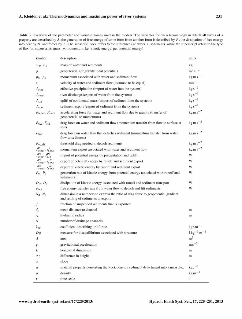
Table 3. Overview of the parameter and variable names used in the models. The variables follow a terminology in which all fluxes of aproperty are described by J , the generation of free energy of some form from another form is described by P , the dissipation of free energyinto heat by D, and forces by F . The subscript index refers to the substance (w: water, s: sediment), while the superscript refers to the typeof flux (no superscript: mass; p: momentum; ke: kinetic energy; pe: potential energy).
symbol description units
mw, ms mass of water and sediments kgφ geopotential (or gravitational potential) m2 s−2
pw, ps momentum associated with water and sediment flow kgm s−1
v velocity of water and sediment flow (assumed to be equal) m s−1
Jw,in effective precipitation (import of water into the system) kg s−1
Jw,out river discharge (export of water from the system) kg s−1
Js,in uplift of continental mass (import of sediment into the system) kg s−1
Js,out sediment export (export of sediment from the system) kg s−1
Fw,acc, Fs,acc accelerating force for water and sediment flow due to gravity (transfer of kgm s−2geopotential to momentum)
Fw,d,Fs,d drag force on water and sediment flow (momentum transfer from flow to surface at kgm s−2rest)
Fw,s drag force on water flow that detaches sediment (momentum transfer from water kgm s−2flow to sediment)
Fw,crit threshold drag needed to detach sediments kgm s−2
Jpw,out, J
ps,out momentum export associated with water and sediment flow kgm s−2
Jpew,in, J
pes,in import of potential energy by precipitation and uplift W
Jpew,out, J
pes,out export of potential energy by runoff and sediment export W
Jkew,out, J
kes,out export of kinetic energy by runoff and sediment export W
Pw, Ps generation rate of kinetic energy from potential energy associated with runoff and Wsediments
Dw, Ds dissipation of kinetic energy associated with runoff and sediment transport WPw,s free energy transfer rate from water flow to detach and lift sediments WNd, Ns dimensionless numbers to express the ratio of drag force to geopotential gradient
and settling of sediments to exportf fraction of suspended sediments that is exporteddc mean distance to channel mrc hydraulic radius mN number of drainage channelskup coefficient describing uplift rate kg sm−1
Dφ measure for disequilibrium associated with structure J kg−1 m−1
A area m2
g gravitational acceleration m s−2
L horizontal dimension m�z difference in height mα slope ◦
µ material property converting the work done on sediment detachment into a mass flux kg J−1
ρ density kgm−3
τ time scale s
www.hydrol-earth-syst-sci.net/17/225/2013/ Hydrol. Earth Syst. Sci., 17, 225–251, 2013
232 A. Kleidon et al.: Thermodynamics and maximum power of river systems
land
atmosphere
ocean land
mantle
crust
atmosphere
ocean
lifter:conversion of kinetic
energy of plate motioninto potential energy of
continental crust
conversion of differential heating and cooling in the interior into kinetic energy of
the crust
heat engine:
transporter:conversion of potential
and chemical free energy of precipitation into kinetic energy of
particulate and dissolved material
conversion of the kinetic energy of
atmospheric motion into potential and
chemical free energy of water vapor
desalinator:
conversion of radiative heating gradients into
kinetic energy associated with
atmospheric motion
heat engine:
warm cold
M
M
atmosphere
landcrust
generation of radiative heating gradients by
solar irradiation
driver:
generation of heating gradients by secular cooling
and radioactive decay
driver:
dynamics of the land surface
M
M
pow
er
pow
er
power
power
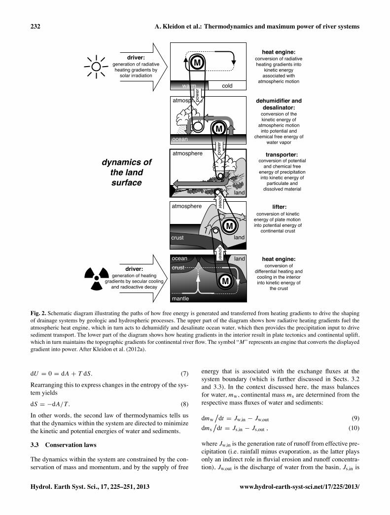
Fig. 2. Schematic diagram illustrating the paths of how free energy is generated and transferred from heating gradients to drive the shapingof drainage systems by geologic and hydrospheric processes. The upper part of the diagram shows how radiative heating gradients fuel theatmospheric heat engine, which in turn acts to dehumidify and desalinate ocean water, which then provides the precipitation input to drivesediment transport. The lower part of the diagram shows how heating gradients in the interior result in plate tectonics and continental uplift,which in turn maintains the topographic gradients for continental river flow. The symbol “M” represents an engine that converts the displayedgradient into power. After Kleidon et al. (2012a).
dU = 0 = dA + T dS. (7)
Rearranging this to express changes in the entropy of the sys-tem yields
dS = −dA/T . (8)
In other words, the second law of thermodynamics tells usthat the dynamics within the system are directed to minimizethe kinetic and potential energies of water and sediments.
3.3 Conservation laws
The dynamics within the system are constrained by the con-servation of mass and momentum, and by the supply of free
energy that is associated with the exchange fluxes at thesystem boundary (which is further discussed in Sects. 3.2and 3.3). In the context discussed here, the mass balancesfor water, mw, continental mass ms are determined from therespective mass fluxes of water and sediments:
dmw�dt = Jw,in − Jw,out (9)
dms�dt = Js,in − Js,out , (10)
where Jw,in is the generation rate of runoff from effective pre-cipitation (i.e. rainfall minus evaporation, as the latter playsonly an indirect role in fluvial erosion and runoff concentra-tion), Jw,out is the discharge of water from the basin, Js,in is
Hydrol. Earth Syst. Sci., 17, 225–251, 2013 www.hydrol-earth-syst-sci.net/17/225/2013/
A. Kleidon et al.: Thermodynamics and maximum power of river systems 233
Δz
LL
ps v
pw v
mw φ
ms φ
rainfall adds mass Jw,in
at φin
uplift adds mass Js,in
at φin
sediment export removes mass Js,out at
φout and v
river discharge removes mass Jw,out at
φout and v
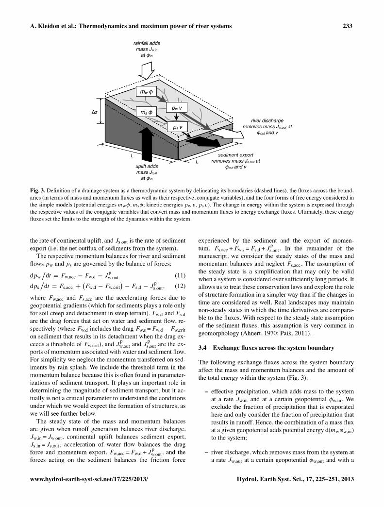
Fig. 3. Definition of a drainage system as a thermodynamic system by delineating its boundaries (dashed lines), the fluxes across the bound-aries (in terms of mass and momentum fluxes as well as their respective, conjugate variables), and the four forms of free energy considered inthe simple models (potential energies mwφ, msφ; kinetic energies pw v, ps v). The change in energy within the system is expressed throughthe respective values of the conjugate variables that convert mass and momentum fluxes to energy exchange fluxes. Ultimately, these energyfluxes set the limits to the strength of the dynamics within the system.
the rate of continental uplift, and Js,out is the rate of sedimentexport (i.e. the net outflux of sediments from the system).The respective momentum balances for river and sediment
flows pw and ps are governed by the balance of forces:
dpw�dt = Fw,acc − Fw,d − J
pw,out (11)
dps�dt = Fs,acc +
�Fw,d − Fw,crit
�− Fs,d − J
ps,out, (12)
where Fw,acc and Fs,acc are the accelerating forces due togeopotential gradients (which for sediments plays a role onlyfor soil creep and detachment in steep terrain), Fw,d and Fs,dare the drag forces that act on water and sediment flow, re-spectively (where Fw,d includes the drag Fw,s =Fw,d− Fw,criton sediment that results in its detachment when the drag ex-ceeds a threshold of Fw,crit), and J
pw,out and J
ps,out are the ex-
ports of momentum associated with water and sediment flow.For simplicity we neglect the momentum transferred on sed-iments by rain splash. We include the threshold term in themomentum balance because this is often found in parameter-izations of sediment transport. It plays an important role indetermining the magnitude of sediment transport, but it ac-tually is not a critical parameter to understand the conditionsunder which we would expect the formation of structures, aswe will see further below.The steady state of the mass and momentum balances
are given when runoff generation balances river discharge,Jw,in = Jw,out, continental uplift balances sediment export,Js,in = Js,out, acceleration of water flow balances the dragforce and momentum export, Fw,acc =Fw,d + J
pw,out, and the
forces acting on the sediment balances the friction force
experienced by the sediment and the export of momen-tum, Fs,acc +Fw,s =Fs,d + J
ps,out. In the remainder of the
manuscript, we consider the steady states of the mass andmomentum balances and neglect Fs,acc. The assumption ofthe steady state is a simplification that may only be validwhen a system is considered over sufficiently long periods. Itallows us to treat these conservation laws and explore the roleof structure formation in a simpler way than if the changes intime are considered as well. Real landscapes may maintainnon-steady states in which the time derivatives are compara-ble to the fluxes. With respect to the steady state assumptionof the sediment fluxes, this assumption is very common ingeomorphology (Ahnert, 1970; Paik, 2011).
3.4 Exchange fluxes across the system boundary
The following exchange fluxes across the system boundaryaffect the mass and momentum balances and the amount ofthe total energy within the system (Fig. 3):
– effective precipitation, which adds mass to the systemat a rate Jw,in and at a certain geopotential φw,in. Weexclude the fraction of precipitation that is evaporatedhere and only consider the fraction of precipitation thatresults in runoff. Hence, the combination of a mass fluxat a given geopotential adds potential energy d(mwφw,in)to the system;
– river discharge, which removes mass from the system ata rate Jw,out at a certain geopotential φw,out and with a
www.hydrol-earth-syst-sci.net/17/225/2013/ Hydrol. Earth Syst. Sci., 17, 225–251, 2013
234 A. Kleidon et al.: Thermodynamics and maximum power of river systems
certain momentum pw. This flux removes geopotentialenergy d(mwφw,out) and kinetic energy d(pw vw) fromthe system;
– continental uplift, which adds continental mass to thesystem at a rate Js,in at a certain geopotential φs,in. Thisaddition of mass at a given geopotential adds potentialenergy d(msφs,in) to the system;
– sediment export associated with river discharge, whichremoves mass from the system at a rate Js,out at a cer-tain geopotential φs,out (=φw,out) and with a certain mo-mentum ps. Sediment export hence exports potentiald(msφs,out) and kinetic energy d(ps vs) from the system.
For simplicity, we assume φin =φw,in =φs,in (we considerthe input of water and sediment at the surface at the sameelevation) and φout =φw,out =φs,out in the following.Since the heat balance does not play a central role for the
dynamics of drainage systems, we do not consider the wholeset of heat fluxes that shape the balances for temperature andentropy, d(T S), within the system. However, we will keeptrack of the dissipation within the system. Furthermore, weneglect the import of momentum associated with the uplift ofcontinental crust.
3.5 Dynamics within the system and its relation toenergy conversions
The hydrologic and geomorphic processes within the systemrelate to the conversions of potential energy that is addedto the system by Jw,in and Js,in to kinetic energy which isexported from the system by Jw,out and Js,out with a lowerpotential energy. Additionally, some of the kinetic energy isconverted to heat. In a simplified treatment we need to ac-count for at least the following processes:
– generation of motion associated with water flow, re-sulting from an accelerating force Fw,acc, at the ex-pense of depleting its potential energy. That is, the po-tential energy d(mwφin) is converted into kinetic en-ergy of the form d(pw vw). When we consider theclassical definition of mechanical work as dW =F dx,with dW = d(mwφin), this yields the well-known ex-pression for gravitational acceleration along the slopewith an angle α of Fw,acc =∇(mwφin)=mw g sin α ≈mw g�z/L;
– frictional dissipation of water flow Dw, associated witha drag force Fw,d, which is driven by the velocity gra-dient ∇v between the water flow and the resting, conti-nental crust. In other words, some of the kinetic energyd(pw vw) is converted into heat d(T S);
– the drag force Fw,s due to the difference in velocities ofthe water flow and the sediment performs work on thesediment. This work entails, e.g. overcoming of bind-ing forces of the sediment, the lifting of sediment into
the water flow, the acceleration to the speed of the flowand its maintenance in suspension against gravity. Thatis, some of the kinetic energy of the water flow d(pw v)is converted to kinetic energy of the sediment d(ps v),and, to some extent, potential energy and the reduc-tion of (negative) binding energy (the latter two con-tributions are neglected here). The partitioning of Fw,son the different forms of work performed on the sedi-ments depends on material properties of the sediments,slope and on the utilization of available transport capac-ity. In the following, we assume that a constant thresh-old stress Fw,crit is needed to detach sediment, while theremainder maintains the kinetic energy of the movingsediment. Hence, if Fw,s is smaller than the threshold,no sediment is detached and can be moved;
– frictional dissipation of sediment flow Ds. Similar tofrictional dissipation of water flow, some of the kineticenergy associated with sediment transport is convertedinto heat.
These conversions are characterized by the budget equa-tions of the potential and kinetic energies of water and sed-iments of the basin, (mwφw), (msφs), (pw vw) and (ps vs),respectively. At a minimum, they consist of the followingterms:
d(mwφw)/dt = Jpew,in − Pw − J
pew,out (13)
d(msφs)/dt = Jpes,in − Ps − J
pes,out (14)
d(pw vw)/dt = Pw − Dw − Pw,s − Jkew,out (15)
d(ps vs)/dt = Ps + Pw,s − Ds − Jkes,out. (16)
In these equations, J pew,in describes the import rate of poten-tial energy of water associated with the influx of mass Jw,in ata geopotential φin, Pw describes the conversion of this poten-tial energy into the kinetic energy of water flow, and J
pew,out
describes the export of potential energy due to lateral ex-change at a geopotential φout. Equivalently, J
pes,in describes
the import rate of potential energy by the addition of massJs,in at a geopotential φin associated with continental crustthrough uplift, which is converted into kinetic energy Ps forsediment transport and is depleted by the export of sedimentsJpes,out triggered by the water flow at a potential φout (i.e. itis related to the kinetic energy export J
kes,out associated with
sediment export). The kinetic energy of water flow is drivenby the input of kinetic energy Pw, and is depleted by fric-tional dissipation Dw (related to the friction force Fw,d andthe velocity gradient), the transfer of free energy to sedimenttransport Pw,s (related to the drag force Fw,s and the velocitygradient), and kinetic energy export J kew,out by river discharge.The kinetic energy associated with sediment transport resultsfrom the balance of the free energy input Pw,s, free energy in-put from the conversion of potential energy of the sediment tokinetic energy Ps (which generally plays a minor role, as de-scribed above), frictional dissipation Ds (related to the drag
Hydrol. Earth Syst. Sci., 17, 225–251, 2013 www.hydrol-earth-syst-sci.net/17/225/2013/
A. Kleidon et al.: Thermodynamics and maximum power of river systems 235
force Fs,d and the velocity gradient between the moving andresting sediment), and the export of kinetic energy by fluxJkes,out.These equations express the conservation of mass, mo-
mentum, and energy at a general level for water and sedi-ment flow within a river catchment and act as constraints tothe dynamics. At this general level, we can already identifyenergetic limits to the dynamics that are not apparent fromthe mass and momentum balances. The transfer of kineticenergy from water to sediment flow is driven by a velocitygradient, but at the same time acts to deplete this gradient.Transferring more and more kinetic energy to sediment trans-port would at first increase the rate of sediment transport, buteventually, the decrease in kinetic energy of the water flowwould slow down the overall export of water and sedimentfrom the drainage basin. Once sediment is transported, it canbe arranged into channel networks that have a lower wet-ted perimeter for a given water flow in relation to a uniformsurface, thereby reducing frictional dissipation. It is in thecontext of such simple considerations that we explore threeways of maximizing the power of sediment transport and itsrelation to preferential flow structures in the following.
4 Maximum power in drainage systems and sedimenttransport
We consider three models in the following that deal with thetransfer of free energy from water flow to sediment trans-port (model 1), the effect of rearranging sediments into theform of river channels on the overall power to drive the de-pletion of the topographic gradient (model 2), and the effectof enhanced removal of continental crust by sediment trans-port on continental uplift (model 3). The three models con-sider the mass, momentum, and energy balances in steadystate, i.e. the fluxes are constant and the state variables donot change in time. Furthermore, we assume that vw = vs = v
for simplicity. This implies that we neglect bedload transportand focus on the transport of suspended sediments.
4.1 Model 1: maximum power to drive sediment export
In the first model we consider the generation and dissipationof kinetic energy associated with surface runoff, and howmuch work can be extracted from this flow to drive sedi-ment export from the slope. To do so, we consider the massbalances of water and sediments as well as the momentumbalance for water flow in a steady state. Since we assumevw = vs = v, we need to consider only one momentum bal-ance, so our starting point are the three balance equations formw, pw, and ms.We start with the mass balance for mw, which balances
effective precipitation with the discharge from the slope:
dmw�dt = 0 = Jw,in − mw v/L . (17)
Here, the runoff is expressed as the mass of water on theslope, mw = ρwLW H , with L and W being the length andwidth of the slope and H corresponding to the height of wa-ter. Hence, the formulation of runoff is equal to ρwAv, withA=W H being the cross section of the flow. The mass bal-ance yields an expression for the total mass of water, mw, onthe slope as a function of effective precipitation, Jw,in, andthe flow velocity of runoff, v:
mw = Jw,inL/v. (18)
The momentum balance (Eq. 9) for water yields the flow ve-locity v on the slope:
d(mw v)�dt = 0 = Fw,acc − Fw,d − J
pw,out , (19)
where Fw,d is a drag force on water flow which includes fric-tion and the stress that the water flow applies to the sediment,Fw,s. The accelerating force for water flow on the slope perunit slope length, Fw,acc, depends on the slope (that is, thegeopotential gradient �φ/L) and on the mass of water onthe slope (we neglect the effect of the water column on theoverall geopotential gradient):
Fw,acc = mw g sin α ≈ mw�φ/L = Jw,in�φ/v, (20)
where the approximation is made that for small anglessin α ≈ α ≈ �z/L. The export of momentum from the slope,Jpw,out, is given by the mass export (which equals the importin steady state, Jw,out = Jw,in) at a velocity v:
Jpw,out = (mw v) v/L = Jw,in v. (21)
Without specifying the specific form of the drag force, wecan combine Eqs. (17)–(19) and obtain a quadratic equationfor v as a function of Fw,d:
v2 + Fw,d v
�Jw,in − �φ = 0 (22)
which yields a solution (with the restriction that v ≥ 0) of
v =�F2w,d/
�4J
2w,in
�+ �φ
�1/2− Fw,d/
�2Jw,in
�. (23)
Two limits of this expression can be derived, depending onthe relative magnitude of F 2
w,d/(4J2w,in) and�φ in the root of
Eq. (21). We use the ratio of these two quantities to define adimensionless number Nd:
Nd = Fw,d/�2Jw,in�φ
1/2�. (24)
This dimensionless number expresses the strength of thedrag force in relation to the slope, with a large value of Ndrepresenting strong drag on shallow slopes, while a smallvalue of Nd represents little drag on steep slopes. Then,the root in Eq. (21) is expressed as �φ
1/2(1 + N
2d )1/2 and
can be approximated for the limit of small (Nd≈ 0) andlarge (Nd� 1) values. At the limit of little frictional drag
www.hydrol-earth-syst-sci.net/17/225/2013/ Hydrol. Earth Syst. Sci., 17, 225–251, 2013

236 A. Kleidon et al.: Thermodynamics and maximum power of river systems
(Fw,d≈ 0 and Nd≈ 0), the root can be approximated by�φ
1/2(1 + N
2d )1/2≈ �φ
1/2 �1 + N
2d /2
�≈ �φ
1/2. This ap-proximation yields the limit for the steady state flow velocityof
v ≈ �φ1/2
. (25)
At the other limit of strong drag, Fw,d� 2 Jw,in�φ1/2 and
Nd� 1, the root in Eq. (21) can be approximated by�φ
1/2(1+N
2d )1/2≈ �φ
1/2(Nd+ 1/(2Nd))=Fw,d/(2Jw,in)
+ Jw,in�φ/Fw,d for large Nd. Then, the velocity isapproximately
v ≈�Jw,in/Fw,d
��φ. (26)
In this case the drag force strongly interacts with the flowvelocity and the dependence of the resulting flow velocityon the slope changes from being proportional to �φ
1/2 to�φ. Note that Eq. (23) represents supercritical flow, whileEq. (24) can yield expressions for Chezy or Darcy flow. Thelatter depends on the choice of Fw,d. If Fw,d is a turbulent,frictional force that depends on the flow velocity, this equa-tion would yield the expression for Chezy flow (in which casethe flow velocity would also be proportional to �φ
1/2). IfFw,d is a binding force that does not depend on the flow ve-locity, this equation yields an expression for Darcy flow.Before we explicitly consider the mass balance of sus-
pended sediments, we note that the drag on water flow isneeded to provide the stress to detach sediment and bring itinto suspension. We express detachment as a threshold pro-cess as
Fw,s = Fw,d − Fw,crit, (27)
where Fw,crit is a material-specific threshold stress and Fw,s isthe force involved in detaching sediment. We assume in thefollowing that the critical threshold stress Fw,crit describes thefrictional dissipation of the kinetic energy of water flow thatdoes not relate to the work of sediment detachment, so thatwe do not account for the frictional drag of water flow addi-tionally. The work performed by this force will then yield thepower to detach sediment, Pw,s, which is given by
Pw,s = Fw,s v. (28)
As it requires work to detach sediment, the rate of sedimentdetachment should be directly proportional to this power(Bagnold, 1966). The sediment export rate is then obtainedfrom the mass balance of suspended sediments, which in-volves the detachment work as well as a sedimentation andexport rate:
dms/dt = 0 = µPw,s − ms/τs − ms v/L, (29)
where µ is a material specific parameter which yields themass flux of detached sediment for a given power, τs is atime scale at which sediment remains in suspension, and the
sediment export flux is written as ms v/L. This mass balanceyields a steady state expression for ms of
ms = µPw,s (τsL)/(L + τs v) (30)
and a sediment export rate Js,out of
Js,out = ms v/L = µPw,s v/(L/τs + v) (31)= µ
�Fw,d − Fw,crit
�v2/(L/τs + v) .
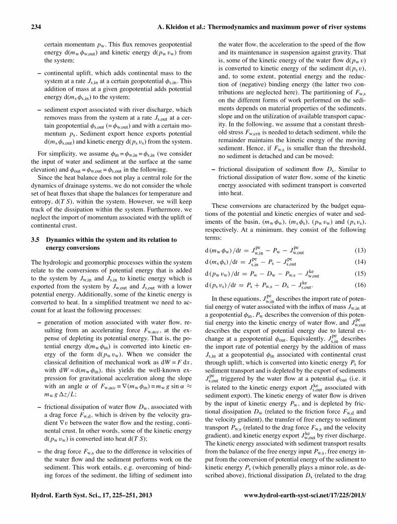
In this expression, both, Pw,s and v, depend on the dragforce, Fw,d, but in opposing ways. While Pw,s increases withFw,d, the terms including v decrease with Fw,d. This re-sults in a maximum possible sediment flux associated withan intermediate value of Fw,d. Figure 4 shows qualitativelythe variation of the different terms as well as the maxi-mum in Js,out as a function of Nd. For the plot, values ofL= 100m, Jw,in = 0.01 kgm−2 s−1, �φ = 1m2 s−2, τs = 10 s,µ= 1 kgm−2 W−1, and Fw,crit = 0.1N were used.We can characterize this maximum in terms of two con-
trasting limitations, the extent to which sediment is detached,and the ability of the water flow to export the sediment. Thesetwo limits are characterized by the ratio of a velocity that isdescribed by the length and time scale of suspended sedi-ments within the system, vs =L/τs, in relation to the velocityof water flow, v, and can be expressed by another dimension-less number Ns, defined by
Ns = vs /v . (32)
The first limit of low sediment deposition (Ns≈ 0, orτs v � L, which means that the effective transport distancebefore settling is much larger than the basin length) repre-sents the case where the power to detach sediment is lim-iting the sediment export flux. At this limit, we obtain theapproximation
Js,out ≈ µPw,s (33)
which represents the limit of low values of Nd in Fig. 4a,because a low drag results in high export ability (as reflectedby the high value of v) while detachment of sediments is lim-ited. The other limit is obtained for large values ofNs. In thiscase, v2/(vs + v) = v (v/vs)/(1 + v/vs) ≈ v
2/vs, and
Js,out ≈ µPw,s v�vs . (34)
This limit is shown for high values of Nd in Fig. 4a, wheredue to the high drag, the low flow velocity limits the exportof sediments from the system.We now trace the power that is provided by the generation
of potential energy by effective precipitation to drive sedi-ment export from the slope. To start, the power generated byeffective precipitation over a geopotential difference �φ isgiven by
Pw = Fw,acc v = Jw,in�φ, (35)
Hydrol. Earth Syst. Sci., 17, 225–251, 2013 www.hydrol-earth-syst-sci.net/17/225/2013/
A. Kleidon et al.: Thermodynamics and maximum power of river systems 237
0
0.2
0.4
0.6
0.8
1.0
0 0.5 1.0 1.5 2.0 2.5 3.0
v
Nd
Pow
er (W
m-2
)Ve
loci
ty (m
s-1
)Fl
ux (k
g m-2
s-1
)
a. Sediment Export
Js,out
Fig. 4b
Pw,s
0.01
0.02
0.05
0.10
0.20
0.50
1.00
0 0.5 1.0 1.5 2.0 2.5 3.0
Pw
Dw
Nd
b. Energetics
Pw,s
J kew,out
Fig. 4c
f Pw,s
Pow
er (W
m-2
)Fl
ux (W
m-2
)D
issi
patio
n (W
m-2
)
Fig. 4. Demonstration of a maximum rate of sediment export result-ing from the tradeoff of increased drag resulting in greater work indetaching sediments, Pw,s, but lower flow velocity, v. (a)Water flowvelocity v, free energy transfer, Pw,s, and rate of sediment export,Js,out, as a function of the dimensionless number, Nd, that charac-terizes the strength of the drag force, Fw,d, in relation to the acceler-ating force, Fw,acc, associated with the slope. (b) Sensitivity of totalpower, Pw, frictional dissipation, Dw, in water flow, kinetic energyexport, J kew,out, of water flow, and the free energy transfer, Pw,s, fromwater flow to sediment transport, and the fraction, f Pw,s, that re-sults in sediment export.
which is the well-known expression for stream power whenconsidered in a channel (Bagnold, 1966). A part of this poweris wasted by frictional loss,Dw, or exported as kinetic energyby runoff, J kew,out, while another part is used to power the de-tachment of sediment, Pw,s:
Dw = Fw,crit v (36)Jkew,out = J
pw,out v = Jw,in v
2 (37)Pw,s =
�Fw,d − Fw,crit
�v. (38)
Of the power available for sediment detachment Pw,s, a frac-tion f = v/(vs + v)= 1/(1 +Ns) results in the actual export ofsediment by the flux Js,out, and the remainder (1− f ) repre-sents the part of the power that is lost when detached sedi-ments are deposited and return to the bed. The different ener-getic terms are shown in Fig. 4b, with the fraction of powerprovided by runoff generation that ends up in sediment ex-port from the slope shown in the graph as f Js,out.
Table 4. Different dependencies of sediment export, Js,out, ongeopotential difference,�φ, (or slope) for different cases of dimen-sionless numbers Nd and Ns.
case drag on sediment sedimentwater export exportflow limitation (Js,out)(Nd) (Ns)
A low low ∝ (�φ)1/2
B low high ∝ (�φ)
C high low ∝ (�φ)
D high high ∝ (�φ)2
The importance of these two limits, as formulated by thetwo dimensionless numbersNd andNs, is that the limits yieldcontrasting dependencies of the sediment export rate Js,out onthe driving gradient, �φ (Table 4). In case A of small valuesof Nd and Ns, which describes conditions of low frictionaldrag and if sediment is being detached, it is easily exported.The expression for the sediment export is obtained by com-bining Eqs. (25) and (33)
Js,out ≈ µFw,s�φ1/2
. (39)
In this case, the rate of sediment export depends on the rootof the slope, Js,out∝ (�φ)
1/2. This case could, for instance,represent the case of the transport of very fine sediment ina channel. In case B of a high value of Nd, but a low valueof Ns, the expression for the sediment export is obtained bycombining Eqs. (26) and (33)
Js,out ≈ µ�Fw,s
�Fw,d
�Jw,in�φ. (40)
Here, Js,out∝ �φ. Case C is represented by a low value ofNd, but a high value of Ns. The expression for the sedimentexport is obtained by combining Eqs. (25) and (34)
Js,out ≈ µ�Fw,s
�vs
��φ. (41)
This case also yields a linear relationship of sediment export,Js,out∝ (�φ), and could represent transport of coarser sedi-ments in a channel. The last case D is obtained by high valuesof Nd and Ns. By combining Eqs. (26) and (34) we obtain
Js,out ≈ µ�Fw,s
�Fw,d
� �Jw,in
�vs
�(�φ)
2. (42)
This case of strong friction and limited ability to export sedi-ments yields Js,out∝ �φ
2. This case is representative of over-land (or subsurface) flow on relatively shallow slopes. As wewill see in the following, this is the most relevant case forstructure formation because the non-uniformity in the slopeenhances the sediment export rate of the slope.In summary, model 1 demonstrates that only a small frac-
tion of the power generated by runoff can be utilized to de-tach and export sediments and thereby deplete the geopo-tential driving gradient of the slope. The existence of a
www.hydrol-earth-syst-sci.net/17/225/2013/ Hydrol. Earth Syst. Sci., 17, 225–251, 2013
238 A. Kleidon et al.: Thermodynamics and maximum power of river systems
maximum in the sediment export rate results from the funda-mental trade-off of increased drag yielding greater sedimentdetachment, but also inevitably reducing the flow velocity atwhich sediment is exported. In the case of such strong inter-actions between water flow and sediment transport, the func-tional dependence of the sediment export rate on the slope isaltered to quadratic form. Even though a maximum rate ofsediment export may not be achieved, it is this case of stronginteraction and non-linear dependence on slope which will beof most relevance for the discussion of structure formation inSect. 5 below.
4.2 Model 2: maximization of sediment export byminimization of frictional losses
Once work is performed on the sediment, mass can be re-arranged to form structures, such as channel networks. Thepresence of channels will affect the intensity of frictionaldrag in model 1, as water flow in a channel has less frictionper unit volume of runoff compared to overland flow becausewater in the channel has, on average, less contact to the solidsurface at rest. In other words, the formation of a channel willresult in shifting the limit of high drag in the case of overlandflow towards less drag and hence towards the case of chan-nel flow. This effectively leads to a lower value of Nd, andthereby alters the relationship between sediment export andthe gradient in geopotential.The model presented here is set up to show that this dif-
ference of flow resistance can minimize frictional dissipationof water flow in the presence of channels, so that sedimentcan be exported at a higher rate and the export limitation as-sociated with overland flow can be reduced. To do so, weconsider a slope of dimension L (length and width) that iswetted uniformly with an effective precipitation Jw,in and onwhich the runoff is discharged from the slope through chan-nels. We assume a constant flow velocity v of water and agiven drag force Fw,d.We start by writing the frictional dissipation rate of the
water flow Dw as the sum of dissipation by overland flow,Dw,o, and channel flow, Dw,c, respectively:
Dw = Dw,o + Dw,c. (43)
The frictional dissipation of overland flow, Dw,o, takes placeacross a contact area of dcL, so that Dw,o can be expressedas
Dw,o ≈ Dw,0 dcL, (44)
where Dw,0 is the constant rate of kinetic energy dissipationof the water flow per unit wetted surface area, dc is the meandistance to the channel, which is dc≈ L/(4N) with N be-ing the number of channels on the slope and dc = 0 as N
approaches infinity (N → ∞). This expression is a simplifi-cation, as it is only an approximation of the actual flow pathsof water to the channel. Note that if we considered subsurface
flow in porous media, the contact area would be substantiallygreater. The actual state of minimum dissipation will be af-fected by such greater contact area, but the existence of aminimum dissipation state should not be affected.The dissipation by channel flow, Dw,c, is approximately
given by the wetted contact area of the perimeter of the chan-nel, π rc, over the length of the slope L:
Dw,c ≈ Dw,0π rcN L, (45)
where rc is the hydraulic radius of the channel, which is as-sumed to be a semicircle for simplicity. This radius rc is de-termined from the constraint that in steady state, the total fluxof water Jw,in is drained through the N channels at bank-fullflow:
Jw,in = N ρw vπ r2c�2 (46)
or
rc =�2Jw,in/(ρw vπ N)
�1/2. (47)
Using Eq. (41) to express rc in Dw,c, we get for the totaldissipation rate Dw:
Dw = Dw,0L2/(4N) + Dw,0
�2π N Jw,in/(ρw v)
�1/2L
= aN−1 + bN
1/2. (48)
This expression of total frictional dissipation exhibits a min-imum value for a certain optimum number of channels, Nopt,due to the tradeoff of a decrease inDw,o asN−1 with a highernumber of channels because the distance, dc, to the nextchannel decreases withN , and an increase inDw,c withN
1/2
because the total wetted perimeter of all channels increaseswith increasing N . This minimum in frictional dissipation,Dw,min, is found with an optimum number of channels, Nopt,to be
Dw,min = (3/2)π1/3Dw,0L4/3 �
Jw,in/(ρw v)�1/3 (49)
and
Nopt = (2a/b)2/3 = L
2/3(8π)
−1/3 �ρw v
�Jw,in
�1/3. (50)
When we express the water inflow as Jw,in = ρi L2, where i
is the effective precipitation intensity, then it follows that theoptimal channel density N
3opt = v/(8π i) depends on the ve-
locity and thus on the slope and the rainfall intensity, i. If thestream velocity does not vary too much, then regions witha high rainfall intensity should have a low optimum channeldensity, while regions with low rainfall intensity should havea high optimum channel density (although channel density isalso affected by other factors such as stage of development).Figure 5 shows qualitatively the variation of the dissi-
pation terms as a function of channel number N and il-lustrates the minimum dissipation state. For the plot, val-ues of L= 1m, Jw,in = 0.01 kgm−2 s−1, ρw = 1000 kgm−3,
Hydrol. Earth Syst. Sci., 17, 225–251, 2013 www.hydrol-earth-syst-sci.net/17/225/2013/
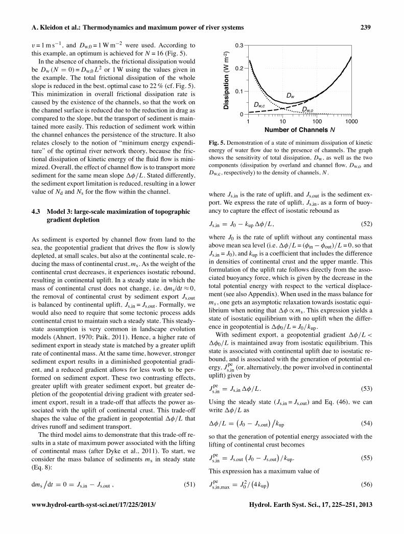
A. Kleidon et al.: Thermodynamics and maximum power of river systems 239
v = 1m s−1, and Dw,0 = 1Wm−2 were used. According tothis example, an optimum is achieved for N = 16 (Fig. 5).In the absence of channels, the frictional dissipation would
be Dw (N = 0)=Dw,0L2 or 1W using the values given inthe example. The total frictional dissipation of the wholeslope is reduced in the best, optimal case to 22% (cf. Fig. 5).This minimization in overall frictional dissipation rate iscaused by the existence of the channels, so that the work onthe channel surface is reduced due to the reduction in drag ascompared to the slope, but the transport of sediment is main-tained more easily. This reduction of sediment work withinthe channel enhances the persistence of the structure. It alsorelates closely to the notion of “minimum energy expendi-ture” of the optimal river network theory, because the fric-tional dissipation of kinetic energy of the fluid flow is mini-mized. Overall, the effect of channel flow is to transport moresediment for the same mean slope �φ/L. Stated differently,the sediment export limitation is reduced, resulting in a lowervalue of Nd and Ns for the flow within the channel.
4.3 Model 3: large-scale maximization of topographicgradient depletion
As sediment is exported by channel flow from land to thesea, the geopotential gradient that drives the flow is slowlydepleted, at small scales, but also at the continental scale, re-ducing the mass of continental crust,ms. As the weight of thecontinental crust decreases, it experiences isostatic rebound,resulting in continental uplift. In a steady state in which themass of continental crust does not change, i.e. dms/dt ≈ 0,the removal of continental crust by sediment export Js,outis balanced by continental uplift, Js,in = Js,out. Formally, wewould also need to require that some tectonic process addscontinental crust to maintain such a steady state. This steady-state assumption is very common in landscape evolutionmodels (Ahnert, 1970; Paik, 2011). Hence, a higher rate ofsediment export in steady state is matched by a greater upliftrate of continental mass. At the same time, however, strongersediment export results in a diminished geopotential gradi-ent, and a reduced gradient allows for less work to be per-formed on sediment export. These two contrasting effects,greater uplift with greater sediment export, but greater de-pletion of the geopotential driving gradient with greater sed-iment export, result in a trade-off that affects the power as-sociated with the uplift of continental crust. This trade-offshapes the value of the gradient in geopotential �φ/L thatdrives runoff and sediment transport.The third model aims to demonstrate that this trade-off re-
sults in a state of maximum power associated with the liftingof continental mass (after Dyke et al., 2011). To start, weconsider the mass balance of sediments ms in steady state(Eq. 8):
dms�dt = 0 = Js,in − Js,out , (51)
0
0.1
0.2
0.3
1 10 100 1000
Fig. 5b
Number of Channels N
Dis
sipa
tion
(W m
-2)
Dw
Dw,oDw,c
Fig. 5. Demonstration of a state of minimum dissipation of kineticenergy of water flow due to the presence of channels. The graphshows the sensitivity of total dissipation, Dw, as well as the twocomponents (dissipation by overland and channel flow, Dw,o andDw,c, respectively) to the density of channels, N .
where Js,in is the rate of uplift, and Js,out is the sediment ex-port. We express the rate of uplift, Js,in, as a form of buoy-ancy to capture the effect of isostatic rebound as
Js,in = J0 − kup�φ/L, (52)
where J0 is the rate of uplift without any continental massabove mean sea level (i.e.�φ/L= (φin − φout)/L= 0, so thatJs,in = J0), and kup is a coefficient that includes the differencein densities of continental crust and the upper mantle. Thisformulation of the uplift rate follows directly from the asso-ciated buoyancy force, which is given by the decrease in thetotal potential energy with respect to the vertical displace-ment (see also Appendix). When used in the mass balance forms , one gets an asymptotic relaxation towards isostatic equi-librium when noting that �φ ∝ ms. This expression yields astate of isostatic equilibrium with no uplift when the differ-ence in geopotential is �φ0/L= J0/kup.With sediment export, a geopotential gradient �φ/L <
�φ0/L is maintained away from isostatic equilibrium. Thisstate is associated with continental uplift due to isostatic re-bound, and is associated with the generation of potential en-ergy, J pes,in (or, alternatively, the power involved in continentaluplift) given by
Jpes,in = Js,in�φ/L. (53)
Using the steady state (Js,in = Js,out) and Eq. (46), we canwrite �φ/L as
�φ/L =�J0 − Js,out
��kup (54)
so that the generation of potential energy associated with thelifting of continental crust becomes
Jpes,in = Js,out
�J0 − Js,out
�/kup. (55)
This expression has a maximum value of
Jpes,in,max = J
20 /
�4kup
�(56)
www.hydrol-earth-syst-sci.net/17/225/2013/ Hydrol. Earth Syst. Sci., 17, 225–251, 2013
240 A. Kleidon et al.: Thermodynamics and maximum power of river systems
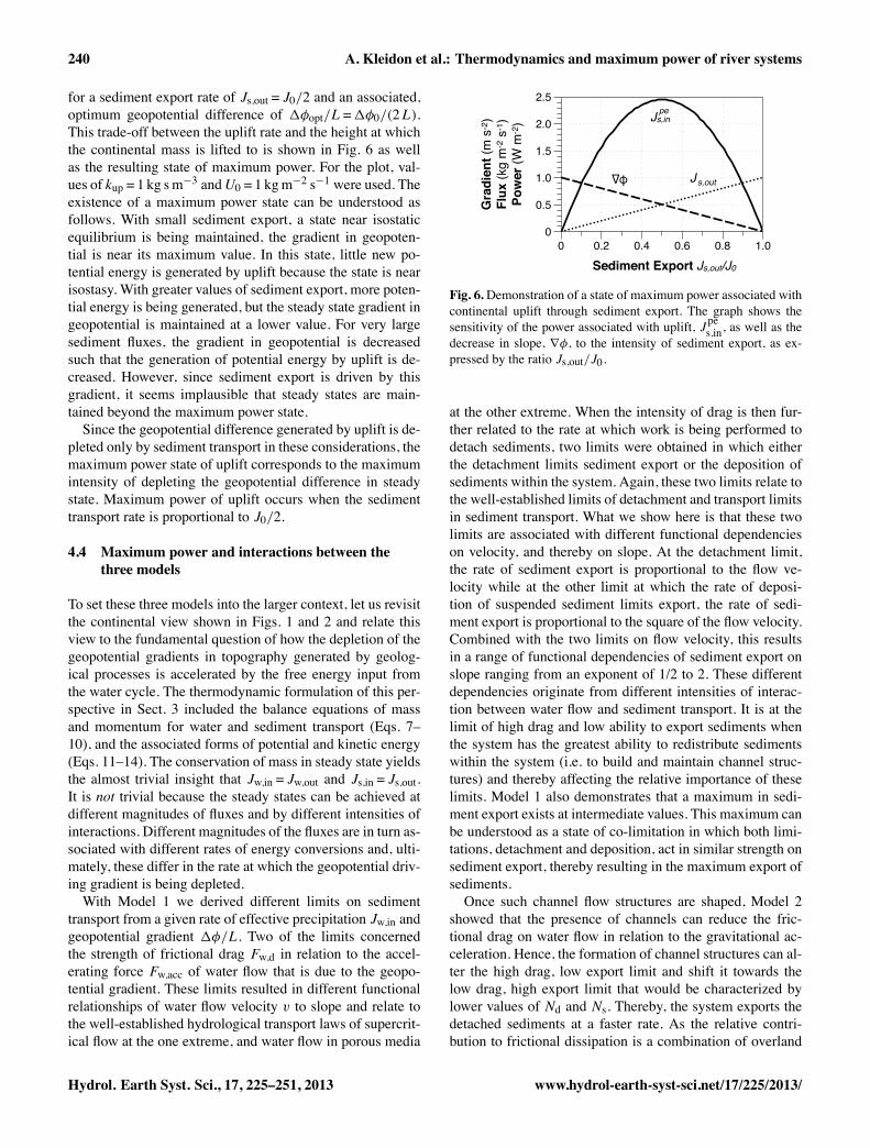
for a sediment export rate of Js,out = J0/2 and an associated,optimum geopotential difference of �φopt/L=�φ0/(2L).This trade-off between the uplift rate and the height at whichthe continental mass is lifted to is shown in Fig. 6 as wellas the resulting state of maximum power. For the plot, val-ues of kup = 1 kg sm−3 andU0 = 1 kgm−2 s−1 were used. Theexistence of a maximum power state can be understood asfollows. With small sediment export, a state near isostaticequilibrium is being maintained, the gradient in geopoten-tial is near its maximum value. In this state, little new po-tential energy is generated by uplift because the state is nearisostasy. With greater values of sediment export, more poten-tial energy is being generated, but the steady state gradient ingeopotential is maintained at a lower value. For very largesediment fluxes, the gradient in geopotential is decreasedsuch that the generation of potential energy by uplift is de-creased. However, since sediment export is driven by thisgradient, it seems implausible that steady states are main-tained beyond the maximum power state.Since the geopotential difference generated by uplift is de-
pleted only by sediment transport in these considerations, themaximum power state of uplift corresponds to the maximumintensity of depleting the geopotential difference in steadystate. Maximum power of uplift occurs when the sedimenttransport rate is proportional to J0/2.
4.4 Maximum power and interactions between thethree models
To set these three models into the larger context, let us revisitthe continental view shown in Figs. 1 and 2 and relate thisview to the fundamental question of how the depletion of thegeopotential gradients in topography generated by geolog-ical processes is accelerated by the free energy input fromthe water cycle. The thermodynamic formulation of this per-spective in Sect. 3 included the balance equations of massand momentum for water and sediment transport (Eqs. 7–10), and the associated forms of potential and kinetic energy(Eqs. 11–14). The conservation of mass in steady state yieldsthe almost trivial insight that Jw,in = Jw,out and Js,in = Js,out.It is not trivial because the steady states can be achieved atdifferent magnitudes of fluxes and by different intensities ofinteractions. Different magnitudes of the fluxes are in turn as-sociated with different rates of energy conversions and, ulti-mately, these differ in the rate at which the geopotential driv-ing gradient is being depleted.With Model 1 we derived different limits on sediment
transport from a given rate of effective precipitation Jw,in andgeopotential gradient �φ/L. Two of the limits concernedthe strength of frictional drag Fw,d in relation to the accel-erating force Fw,acc of water flow that is due to the geopo-tential gradient. These limits resulted in different functionalrelationships of water flow velocity v to slope and relate tothe well-established hydrological transport laws of supercrit-ical flow at the one extreme, and water flow in porous media
Jpes,in
∇φ Js,out
0
0.5
1.0
1.5
2.0
2.5
0 0.2 0.4 0.6 0.8 1.0
Fig. 6b
Sediment Export Js,out/J0
Gra
dien
t (m
s-2
)Fl
ux (k
g m-2
s-1
)Po
wer
(W m
-2)
∇φ Js,out
Js,inpe
Fig. 6. Demonstration of a state of maximum power associated withcontinental uplift through sediment export. The graph shows thesensitivity of the power associated with uplift, J pes,in, as well as thedecrease in slope, ∇φ, to the intensity of sediment export, as ex-pressed by the ratio Js,out/J0.
at the other extreme. When the intensity of drag is then fur-ther related to the rate at which work is being performed todetach sediments, two limits were obtained in which eitherthe detachment limits sediment export or the deposition ofsediments within the system. Again, these two limits relate tothe well-established limits of detachment and transport limitsin sediment transport. What we show here is that these twolimits are associated with different functional dependencieson velocity, and thereby on slope. At the detachment limit,the rate of sediment export is proportional to the flow ve-locity while at the other limit at which the rate of deposi-tion of suspended sediment limits export, the rate of sedi-ment export is proportional to the square of the flow velocity.Combined with the two limits on flow velocity, this resultsin a range of functional dependencies of sediment export onslope ranging from an exponent of 1/2 to 2. These differentdependencies originate from different intensities of interac-tion between water flow and sediment transport. It is at thelimit of high drag and low ability to export sediments whenthe system has the greatest ability to redistribute sedimentswithin the system (i.e. to build and maintain channel struc-tures) and thereby affecting the relative importance of theselimits. Model 1 also demonstrates that a maximum in sedi-ment export exists at intermediate values. This maximum canbe understood as a state of co-limitation in which both limi-tations, detachment and deposition, act in similar strength onsediment export, thereby resulting in the maximum export ofsediments.Once such channel flow structures are shaped, Model 2
showed that the presence of channels can reduce the fric-tional drag on water flow in relation to the gravitational ac-celeration. Hence, the formation of channel structures can al-ter the high drag, low export limit and shift it towards thelow drag, high export limit that would be characterized bylower values of Nd and Ns. Thereby, the system exports thedetached sediments at a faster rate. As the relative contri-bution to frictional dissipation is a combination of overland
Hydrol. Earth Syst. Sci., 17, 225–251, 2013 www.hydrol-earth-syst-sci.net/17/225/2013/
A. Kleidon et al.: Thermodynamics and maximum power of river systems 241
and channel flow, a minimum in frictional loss can be ob-tained at a certain channel density N . This optimum channeldensity decreases with increasing mass of water that is to beexported. Hence, as larger and larger continental regions arebeing considered that drain greater volumes of water and sed-iments, the formation of greater and fewer drainage channelscan reduce the frictional losses further, and thus enhance sed-iment export and the depletion of continental-scale geopoten-tial gradients.With increasing values of sediment export, the geopo-
tential gradient is brought further and further awayfrom a state of isostatic equilibrium. That is, the lo-cal, isostatic disequilibrium of the geopotential gradient�φ0/L − �φ/L= Js,out/kup (cf. Eq. 46) increases with in-creasing values of Js,out, and results in greater rates of conti-nental uplift. This reduction in gradient, however, inevitablyreduces the power Pw and Ps that drive sediment export.Model 3 showed that through adjustments in the intensity ofsediment export, continental uplift can be maintained in astate of maximum power at which the generation rate of po-tential energy of continental crust at the surface is at a max-imum. Through this effect, the driving gradient for sedimenttransport, �φ/L, is maintained at a higher value in steadystate than in the absence of isostatic rebound.In summary, the three models taken together sketch out
how the input of free energy by the continental water cyclecan accelerate the dynamics that deplete the state of isostaticequilibrium of the continental crust (Fig. 1b) towards a stateof global equilibrium (Fig. 1d). This acceleration of conti-nental sediment export is not arbitrary, but strictly bound byupper limits on how much free energy can be transferredfrom runoff to sediment transport and from isostatic rebound.Furthermore, the reduction in frictional dissipation associ-ated with channel flow provides a means to understand howthe overall system could achieve such an optimum state atwhich these upper limits are reached. This leaves the ques-tion as to why the dynamics should progress towards theseupper limits, which we will address in the following section.
5 Evolution towards disequilibrium and maximizationby structure formation
The three models of the previous section establish the lim-its to the dynamics of sediment transport, the importance ofinteractions, and the ingredients to understand how maxi-mization associated with the depletion of geopotential gra-dients could be achieved. We now make the link between thethree models more explicit. We discuss how the evolution ofa drainage system from a uniform slope to a structured basin,as shown in Fig. 7, can be understood as the expected andinevitable outcome of the dynamics that evolve to maximizethe dissipation of the driving geopotential gradient by the ex-port of sediment from the system.
a. initial uniform slope b. perturbation
c. growth d. spread
e. dominance f. feedback
Fig. 7. Six stages of structure formation that reflect increasing lev-els of disequilibrium and ability to generate free energy and drivesediment transport. See main text for description.
In this example, our use of the term “structure” refersto the spatial, topographic heterogeneity on the slope andincludes the combination of two aspects: (a) the non-uniformity (or heterogeneity) of the geopotential gradients,expressed by the deviation of the local slopes from the meanslope, and (b) the arrangement of these local deviations oc-curs in an ordered way by the ordered, backward-invasiveprocess of channel incision. Hence, our use of “structure”not only includes the connected channel network, but alsothe steepened slopes that frame the channel network. In otherwords, we refer to “structure” as organized heterogeneityalong connective pathways.To do so, we consider a thought experiment, in which we
look at a uniform and homogeneously sloped surface that isclose to isostatic equilibrium and experiences very little up-lift (Fig. 7a). This slope is in a steady-state with respect tothe mass balances of water and sediments, i.e. the net influxof water and sediments into the system balances the exportof runoff and sediments. The sequence of steps of how a
www.hydrol-earth-syst-sci.net/17/225/2013/ Hydrol. Earth Syst. Sci., 17, 225–251, 2013
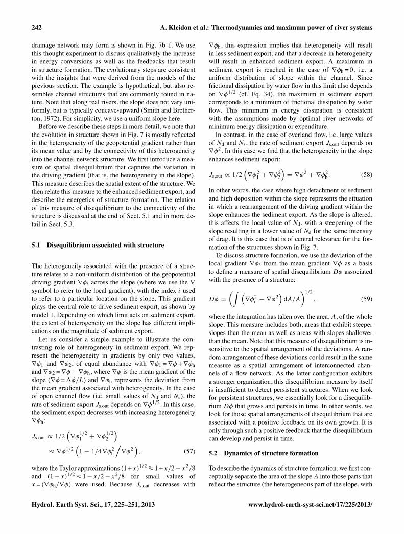
242 A. Kleidon et al.: Thermodynamics and maximum power of river systems
drainage network may form is shown in Fig. 7b–f. We usethis thought experiment to discuss qualitatively the increasein energy conversions as well as the feedbacks that resultin structure formation. The evolutionary steps are consistentwith the insights that were derived from the models of theprevious section. The example is hypothetical, but also re-sembles channel structures that are commonly found in na-ture. Note that along real rivers, the slope does not vary uni-formly, but is typically concave-upward (Smith and Brether-ton, 1972). For simplicity, we use a uniform slope here.Before we describe these steps in more detail, we note that
the evolution in structure shown in Fig. 7 is mostly reflectedin the heterogeneity of the geopotential gradient rather thanits mean value and by the connectivity of this heterogeneityinto the channel network structure. We first introduce a mea-sure of spatial disequilibrium that captures the variation inthe driving gradient (that is, the heterogeneity in the slope).This measure describes the spatial extent of the structure. Wethen relate this measure to the enhanced sediment export, anddescribe the energetics of structure formation. The relationof this measure of disequilibrium to the connectivity of thestructure is discussed at the end of Sect. 5.1 and in more de-tail in Sect. 5.3.
5.1 Disequilibrium associated with structure
The heterogeneity associated with the presence of a struc-ture relates to a non-uniform distribution of the geopotentialdriving gradient ∇φi across the slope (where we use the ∇symbol to refer to the local gradient), with the index i usedto refer to a particular location on the slope. This gradientplays the central role to drive sediment export, as shown bymodel 1. Depending on which limit acts on sediment export,the extent of heterogeneity on the slope has different impli-cations on the magnitude of sediment export.Let us consider a simple example to illustrate the con-
trasting role of heterogeneity in sediment export. We rep-resent the heterogeneity in gradients by only two values,∇φ1 and ∇φ2, of equal abundance with ∇φ1 =∇φ +∇φhand ∇φ2 =∇φ − ∇φh, where ∇φ is the mean gradient of theslope (∇φ =�φ/L) and ∇φh represents the deviation fromthe mean gradient associated with heterogeneity. In the caseof open channel flow (i.e. small values of Nd and Ns), therate of sediment export Js,out depends on ∇φ
1/2. In this case,the sediment export decreases with increasing heterogeneity∇φh:
Js,out ∝ 1/2�∇φ
1/21 + ∇φ
1/22
�
≈ ∇φ1/2
�1 − 1/4∇φ
2h
�∇φ
2�, (57)
where the Taylor approximations (1 + x)1/2≈ 1 + x/2− x
2/8
and (1− x)1/2≈ 1− x/2− x
2/8 for small values of
x = (∇φh/∇φ) were used. Because Js,out decreases with
∇φh, this expression implies that heterogeneity will resultin less sediment export, and that a decrease in heterogeneitywill result in enhanced sediment export. A maximum insediment export is reached in the case of ∇φh = 0, i.e. auniform distribution of slope within the channel. Sincefrictional dissipation by water flow in this limit also dependson ∇φ
1/2 (cf. Eq. 34), the maximum in sediment exportcorresponds to a minimum of frictional dissipation by waterflow. This minimum in energy dissipation is consistentwith the assumptions made by optimal river networks ofminimum energy dissipation or expenditure.In contrast, in the case of overland flow, i.e. large values
of Nd and Ns, the rate of sediment export Js,out depends on∇φ
2. In this case we find that the heterogeneity in the slopeenhances sediment export:
Js,out ∝ 1/2�∇φ
21 + ∇φ
22
�= ∇φ
2 + ∇φ2h . (58)
In other words, the case where high detachment of sedimentand high deposition within the slope represents the situationin which a rearrangement of the driving gradient within theslope enhances the sediment export. As the slope is altered,this affects the local value of Nd, with a steepening of theslope resulting in a lower value of Nd for the same intensityof drag. It is this case that is of central relevance for the for-mation of the structures shown in Fig. 7.To discuss structure formation, we use the deviation of the
local gradient ∇φi from the mean gradient ∇φ as a basisto define a measure of spatial disequilibrium Dφ associatedwith the presence of a structure:
Dφ =�� �
∇φ2i
− ∇φ2�dA/A
�1/2, (59)
where the integration has taken over the area,A, of the wholeslope. This measure includes both, areas that exhibit steeperslopes than the mean as well as areas with slopes shallowerthan the mean. Note that this measure of disequilibrium is in-sensitive to the spatial arrangement of the deviations. A ran-dom arrangement of these deviations could result in the samemeasure as a spatial arrangement of interconnected chan-nels of a flow network. As the latter configuration exhibitsa stronger organization, this disequilibrium measure by itselfis insufficient to detect persistent structures. When we lookfor persistent structures, we essentially look for a disequilib-rium Dφ that grows and persists in time. In other words, welook for those spatial arrangements of disequilibrium that areassociated with a positive feedback on its own growth. It isonly through such a positive feedback that the disequilibriumcan develop and persist in time.
5.2 Dynamics of structure formation
To describe the dynamics of structure formation, we first con-ceptually separate the area of the slopeA into those parts thatreflect the structure (the heterogeneous part of the slope, with
Hydrol. Earth Syst. Sci., 17, 225–251, 2013 www.hydrol-earth-syst-sci.net/17/225/2013/

A. Kleidon et al.: Thermodynamics and maximum power of river systems 243
both, steeper and shallower slopes than the mean), Astructure,and those of the remaining parts of the slope (the uniformpart of the slope), Aslope:
A = Astructure + Aslope. (60)
The spatial extent of the structure, Astructure, represents thoseareas in which the local slope deviates from the mean slopeby a certain threshold value and thus includes the channelnetwork. Then, the sediment export characteristics of thewhole slope can be separated into the contribution to the totalsediment export by the structure, Js,out,structure and by the sed-iment export of the mean properties of the slope, Js,out,slopefor the remaining area Aslope.Since the sediment export from the structure, i.e. the com-
bination of steeper hillslopes and less steep channels, is onaverage greater than the export from the remaining slope, thedepletion of potential energy of the sediment should differ.Hence, we separate the depletion of potential energy into twoterms, one representing the depletion of the potential energyof the structure, (msφs)structure, and one for the remainingslope, (msφs)slope:
d(msφs)�dt = d (msφs)structure
�dt + d (msφs)slope
�dt . (61)
We can then further express the individual changes of poten-tial energy by
d(msφs)structure�dt =
�Js,inφin − Js,out,structureφout
�Astructure
�A (62)
and
d(msφs)slope�dt =
�Js,inφin − Js,out,slopeφout
�Aslope
�A ,(63)
where we assume that both components are governed by thesame rate of uplift, Js,in, but differ in their rates of sedimentexport.Since the initial state of the slope shown in Fig. 7a most
likely represents the case of overland flow, the rate of sedi-ment export will be proportional to ∇φ
2i. Because the struc-
ture by definition reflects the part of the slope with hetero-geneity, it will have a greater rate of sediment export, so thatthe depletion rate of potential energy of the structure shouldproceed at a greater rate than that of the remaining slope.That is, |d(msφs)structure/dt | > |d(msφs)slope/dt |, with thedifference between the two rates being roughly proportionalto Dφ
2. On the other hand, the different rates of change in(msφs)structure and (msφs)slope affect the topographic gradi-ent and the spatial extent of the structure and the surroundingslope, so that this should result in accompanying changes inthe areal extent of the structure, Astructure, and the state ofdisequilibrium, Dφ, of the slope.
5.3 Evolution towards greater disequilibrium andstructure
The evolutionary trend in Fig. 7 is characterized by the arealextent of the channel network structure, Astructure, and its dis-equilibrium,Dφ. The different stages should furthermore re-flect clear and consistent trends in the variables that reflectthe intensity by which the geopotential gradient is depleted.These include the reduction of frictional dissipation of waterflow by overland flow because increasingly more water is ex-ported from the slope through the channel network, which iscaptured by the two variables Dw,o and Dw,c. The steepenedslopes at the boundary of the structure as well as the reducedfrictional dissipation within the channel network of the struc-ture should result in more work done to detach sedimentson the steepened slopes and more efficient export of sedi-ments by channel flow from the slope, which is captured bythe variables Js,out,structure and Js,out,slope. The trends in thesevariables is sketched qualitatively in Fig. 8 and described inmore detail in the following.Stage 1: uniformity (Fig. 7a). The initially uniform and ho-
mogeneously sloped surface has a uniform gradient in geopo-tential, so that ∇φi =∇φ at every location i, so that Dφ = 0.Hence, the runoff generated from incoming precipitation ex-periences the same, high drag throughout the slope whichis characterized by a high value of Nd. The resulting waterflow is dissipated entirely by overland flow as no channelsare present, i.e. Dw =Dw,o. As shown in model 2 above, thisconfiguration of flow has the greatest contact with the sed-iment at the surface and experiences the greatest frictionaldissipation. With the greatest intensity of friction, the forcesacting on the sediment are greatest as well, but because ofthe resulting slow flow velocity of overland flow, the actualtransport of sediments is small. Hence, little of the continen-tal mass is transported downslope by the flow, and if so, onlyfor a short distance. Overall, this results in little export of ki-netic energy of the overland flow as well as little sediment ex-port from the slope (Js,out≈ 0). In steady state, this small fluxof sediment export would be balanced by a small rate of con-tinental uplift (Js,in≈ 0), which would involve little power tosustain (J pes,in≈ 0).Stage 2: perturbation (Fig. 7b). We now consider a random
perturbation that leads to the removal of some sediment froma small area on the slope. This removal has the greatest prob-ability to occur at the lower end of the slope, as this is theplace where the highest flux of water per unit cross sectionoccurs. It could, however, also occur further upslope, or at adifferent location along the slope since we consider a randomperturbation. Such a perturbation would lead to a steepen-ing of the local slope, so that ∇φj > ∇φ for this location j .Our measure for disequilibrium becomes greater than zero,Dφ > 0 and the area of the structure, while small, starts to begreater than zero, Astructure> 0. Since the conditions of dragand sediment transport are characterized by high values ofNd and Ns, sediment export is proportional to (∇φj )
2. This
www.hydrol-earth-syst-sci.net/17/225/2013/ Hydrol. Earth Syst. Sci., 17, 225–251, 2013

244 A. Kleidon et al.: Thermodynamics and maximum power of river systems
local steepening of the slope hence results in disproportionalenhancement of sediment transport from the perturbed areaand the local enhancement of sediment export should act toenhance the growth of the perturbation.Stage 3: growth (Fig. 7c). The enhanced sediment export
from the locally steepened slope has two important conse-quences: first, it forms a positive feedback on the growth ofthis perturbation. When the locally enhanced export removesmaterial from the steepened slope, it pushes the steepenedslope further upslope, where more sediment can be removed.This then acts to enhance the perturbation in spatial extent,resulting in larger values of Astructure and Dφ. Second, thearea downslope of the steepened slope represents a confinedspatial channel structure with a reduced gradient within thechannel structure and a reduced contact area to volume flowratio. That is, drag is reduced, the value of Nd is decreased,while enhancing the ability to export sediment, i.e. the valueof Ns is reduced as well. Overall, this results in an enhancedexport of kinetic energy of water flow through the channelas well as enhanced export of sediments within the flow. Assome water is exported by the structure, the frictional dissi-pation by overland flow,Dw,o, is reduced, while the sedimentexport by the structure, Js,out,structure, is enhanced.Stage 4: spread (Fig. 7d). As the steepened slope pro-
gresses to grow further upslope and deepens, the slopes alongthe channel are steepened as well. This steepening of thechannel slopes makes them more susceptible to perturbationsthat remove sediments. The location of such a perturbationwould be another random event, with a higher probability tooccur in areas of steeper slopes. When such a perturbationarises, this perturbation would grow and experience the samepositive feedback as discussed in the previous two steps. Thisis essentially a self-similar process forming self-similar net-work structures and it would act to spread the steepening ofthe gradient in geopotential beyond areas directly upslope ofthe channel, increasing the values of Astructure and Dφ. Thisgrowth of the structure would collect more of the generatedrunoff of the slope, it would generate more work in detachingsediments on the steepened slopes at the edges of the struc-ture, and the channel network within the structure would ex-port water and sediments more effectively. The overall fric-tional dissipation is decreased, withDw,o decreasing substan-tially, while Dw,c slightly increasing simply because morewater is transported by channels. As more work on detach-ing sediments is performed and sediments are exported moreeffectively from the slope, the overall export of sediments,Js,out, should increase due to the increase in Js,out,structure.Stage 5: dominance (Fig. 7e). Eventually, the structure
spreads by the positive feedbacks on growth over the wholeslope. At this point, Astructure≈ A, Aslope≈ 0, and the extentof disequilibrium Dφ has increased further. As the structuregrows in size, it becomes more efficient at exporting runoffand sediments, as discussed in the context of model 2 interms of the sensitivity to Jw,in. This effect results in furtherreduction in frictional losses within the structure, although
the overall dissipation should still somewhat increase dueto the increase in size compared to the previous stage. Atthis stage, the structure composed of steepened gradients atthe edges and reduced gradients within the channel networkdominates the fluvial behavior of the slope. The steepenedslopes at the edges generate more power to provide morework to detach sediments from the slopes. At the same time,the leveling of slope and the reduction in wetted perimeterwithin the channels enhances the overall export of sedimentsfrom the slope. These effects should thus further enhance theoverall export of sediments by the structure, Js,out,structure.Stage 6: feedback (Fig. 7f). As the structure efficiently
erodes and transports the sediment from the slope, its totalmass is reduced and so is its weight. With this reduction ofmass, the mean slope is being reduced, and thereby the driv-ing force for runoff generation and sediment transport. Thisreduction in slope thereby acts as a negative feedback to thegrowth of the structure. On the other hand, the reduction ofweight at sufficiently large scales will bring the elevation outof a state of isostatic equilibrium (cf. Fig. 1), which will en-hance continental uplift to restore the equilibrium height, asshown by model 3. While the overall size of the structure canno longer increase as it already dominates the slope, the dis-equilibrium Dφ can potentially increase further due to thegreater uplift of continental crust. Such an increase in Dφ
could then affect frictional dissipation as it alters the localgradients, and it can further increase the overall export ofsediments from the slope due to the increase in uplift. This,in total, enhances the overall depletion of the topographicgradient between continental and oceanic crust, thereby ac-celerating the evolution to the global equilibrium state shownin Fig. 1d.
5.4 Disequilibrium, structures, and maximization
To sum up, the evolutionary sequence of channel networkformation as shown in Figs. 7 and 8 should follow a con-sistent trend towards greater power for fluvial processes thatare able to enhance the sediment export from the region. Thistrend is accompanied with an evolution towards greater val-ues of spatial disequilibrium, as introduced in Sect. 5.1. Fur-thermore, the dynamics are such that they inevitably result ingreater connectivity of the channel network. At the center ofthis evolutionary sequence are feedbacks that enhance sedi-ment export by the formation of structure. These feedbackswe explore in the following in more detail.
6 Time scales and feedbacks
To better identify the feedbacks that lead to the evolutionarydynamics towards maximization through structure forma-tion, we first introduce two time scales that describe the dy-namics described above. We then relate these time scales tothe dominant feedbacks that are involved in the maximization
Hydrol. Earth Syst. Sci., 17, 225–251, 2013 www.hydrol-earth-syst-sci.net/17/225/2013/
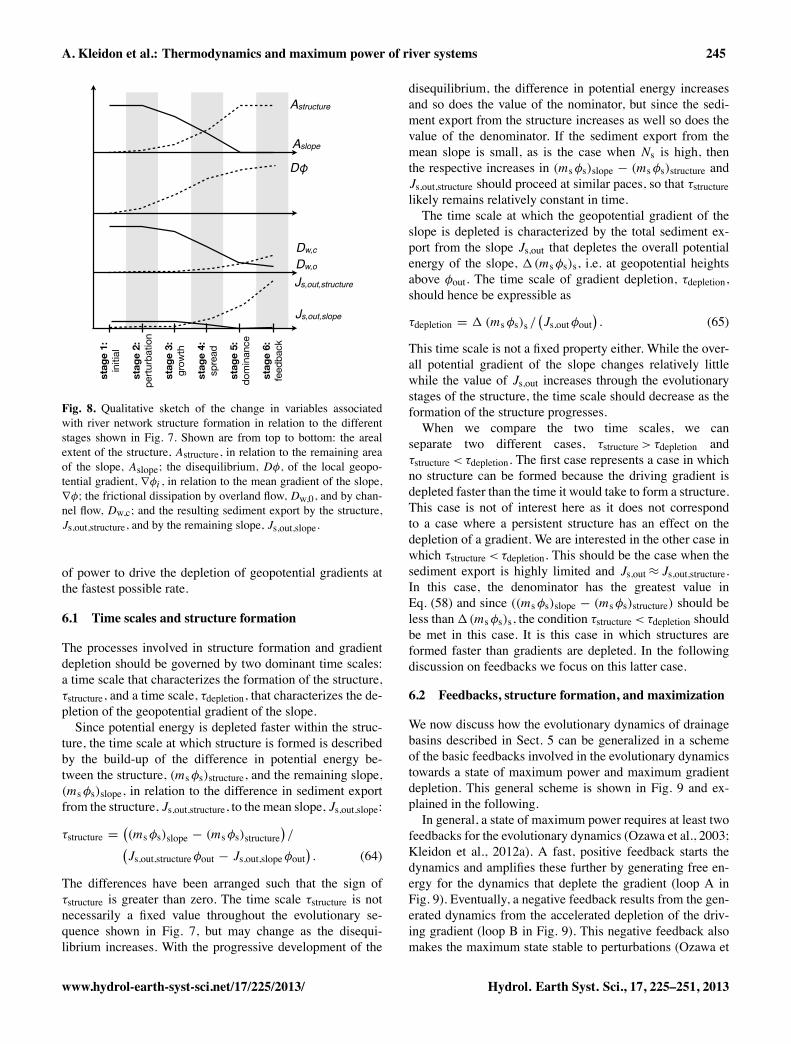
A. Kleidon et al.: Thermodynamics and maximum power of river systems 245
Fig. 8st
age
1:initial
stag
e 2:
perturbation
stag
e 3:
growth
stag
e 4:
spread
stag
e 5:
dominance
stag
e 6:
feedback
Js,out,structure
Astructure
Dφ
Aslope
Js,out,slope
Dw,o
Dw,c
Fig. 8. Qualitative sketch of the change in variables associatedwith river network structure formation in relation to the differentstages shown in Fig. 7. Shown are from top to bottom: the arealextent of the structure, Astructure, in relation to the remaining areaof the slope, Aslope; the disequilibrium, Dφ, of the local geopo-tential gradient, ∇φi , in relation to the mean gradient of the slope,∇φ; the frictional dissipation by overland flow, Dw,0, and by chan-nel flow, Dw,c; and the resulting sediment export by the structure,Js,out,structure, and by the remaining slope, Js,out,slope.
of power to drive the depletion of geopotential gradients atthe fastest possible rate.
6.1 Time scales and structure formation
The processes involved in structure formation and gradientdepletion should be governed by two dominant time scales:a time scale that characterizes the formation of the structure,τstructure, and a time scale, τdepletion, that characterizes the de-pletion of the geopotential gradient of the slope.Since potential energy is depleted faster within the struc-
ture, the time scale at which structure is formed is describedby the build-up of the difference in potential energy be-tween the structure, (msφs)structure, and the remaining slope,(msφs)slope, in relation to the difference in sediment exportfrom the structure, Js,out,structure, to the mean slope, Js,out,slope:
τstructure =�(msφs)slope − (msφs)structure
�/
�Js,out,structureφout − Js,out,slopeφout
�. (64)
The differences have been arranged such that the sign ofτstructure is greater than zero. The time scale τstructure is notnecessarily a fixed value throughout the evolutionary se-quence shown in Fig. 7, but may change as the disequi-librium increases. With the progressive development of the
disequilibrium, the difference in potential energy increasesand so does the value of the nominator, but since the sedi-ment export from the structure increases as well so does thevalue of the denominator. If the sediment export from themean slope is small, as is the case when Ns is high, thenthe respective increases in (msφs)slope − (msφs)structure andJs,out,structure should proceed at similar paces, so that τstructurelikely remains relatively constant in time.The time scale at which the geopotential gradient of the
slope is depleted is characterized by the total sediment ex-port from the slope Js,out that depletes the overall potentialenergy of the slope, �(msφs)s, i.e. at geopotential heightsabove φout. The time scale of gradient depletion, τdepletion,should hence be expressible as
τdepletion = � (msφs)s /�Js,outφout
�. (65)
This time scale is not a fixed property either. While the over-all potential gradient of the slope changes relatively littlewhile the value of Js,out increases through the evolutionarystages of the structure, the time scale should decrease as theformation of the structure progresses.When we compare the two time scales, we can
separate two different cases, τstructure> τdepletion andτstructure< τdepletion. The first case represents a case in whichno structure can be formed because the driving gradient isdepleted faster than the time it would take to form a structure.This case is not of interest here as it does not correspondto a case where a persistent structure has an effect on thedepletion of a gradient. We are interested in the other case inwhich τstructure< τdepletion. This should be the case when thesediment export is highly limited and Js,out≈ Js,out,structure.In this case, the denominator has the greatest value inEq. (58) and since ((msφs)slope − (msφs)structure) should beless than�(msφs)s, the condition τstructure< τdepletion shouldbe met in this case. It is this case in which structures areformed faster than gradients are depleted. In the followingdiscussion on feedbacks we focus on this latter case.
6.2 Feedbacks, structure formation, and maximization
We now discuss how the evolutionary dynamics of drainagebasins described in Sect. 5 can be generalized in a schemeof the basic feedbacks involved in the evolutionary dynamicstowards a state of maximum power and maximum gradientdepletion. This general scheme is shown in Fig. 9 and ex-plained in the following.In general, a state of maximum power requires at least two
feedbacks for the evolutionary dynamics (Ozawa et al., 2003;Kleidon et al., 2012a). A fast, positive feedback starts thedynamics and amplifies these further by generating free en-ergy for the dynamics that deplete the gradient (loop A inFig. 9). Eventually, a negative feedback results from the gen-erated dynamics from the accelerated depletion of the driv-ing gradient (loop B in Fig. 9). This negative feedback alsomakes the maximum state stable to perturbations (Ozawa et
www.hydrol-earth-syst-sci.net/17/225/2013/ Hydrol. Earth Syst. Sci., 17, 225–251, 2013
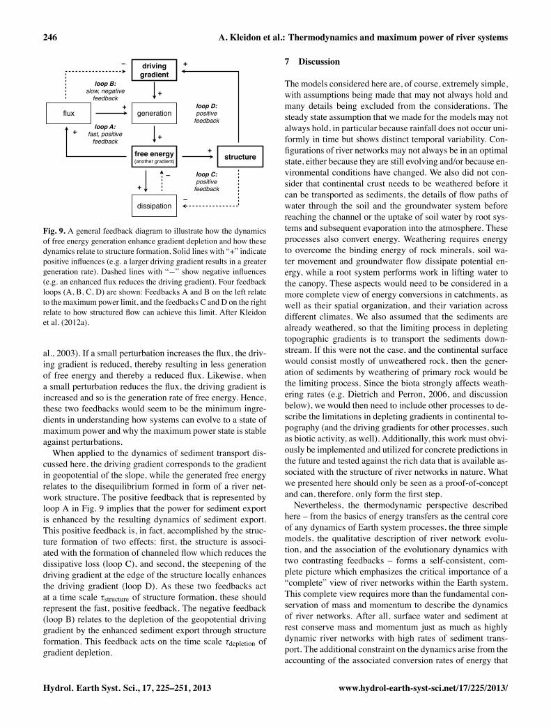
246 A. Kleidon et al.: Thermodynamics and maximum power of river systems
driving gradient
generationflux
free energy(another gradient)
dissipation
structure
+
+
+
+
+
–
–
–
loop B:slow, negative
feedback
loop A: fast, positive
feedback
loop C:positive
feedback
+
+
loop D:positive
feedback
Fig. 9
Fig. 9. A general feedback diagram to illustrate how the dynamicsof free energy generation enhance gradient depletion and how thesedynamics relate to structure formation. Solid lines with “+” indicatepositive influences (e.g. a larger driving gradient results in a greatergeneration rate). Dashed lines with “−” show negative influences(e.g. an enhanced flux reduces the driving gradient). Four feedbackloops (A, B, C, D) are shown: Feedbacks A and B on the left relateto the maximum power limit, and the feedbacks C and D on the rightrelate to how structured flow can achieve this limit. After Kleidonet al. (2012a).
al., 2003). If a small perturbation increases the flux, the driv-ing gradient is reduced, thereby resulting in less generationof free energy and thereby a reduced flux. Likewise, whena small perturbation reduces the flux, the driving gradient isincreased and so is the generation rate of free energy. Hence,these two feedbacks would seem to be the minimum ingre-dients in understanding how systems can evolve to a state ofmaximum power and why the maximum power state is stableagainst perturbations.When applied to the dynamics of sediment transport dis-
cussed here, the driving gradient corresponds to the gradientin geopotential of the slope, while the generated free energyrelates to the disequilibrium formed in form of a river net-work structure. The positive feedback that is represented byloop A in Fig. 9 implies that the power for sediment exportis enhanced by the resulting dynamics of sediment export.This positive feedback is, in fact, accomplished by the struc-ture formation of two effects: first, the structure is associ-ated with the formation of channeled flow which reduces thedissipative loss (loop C), and second, the steepening of thedriving gradient at the edge of the structure locally enhancesthe driving gradient (loop D). As these two feedbacks actat a time scale τstructure of structure formation, these shouldrepresent the fast, positive feedback. The negative feedback(loop B) relates to the depletion of the geopotential drivinggradient by the enhanced sediment export through structureformation. This feedback acts on the time scale τdepletion ofgradient depletion.
7 Discussion
The models considered here are, of course, extremely simple,with assumptions being made that may not always hold andmany details being excluded from the considerations. Thesteady state assumption that we made for the models may notalways hold, in particular because rainfall does not occur uni-formly in time but shows distinct temporal variability. Con-figurations of river networks may not always be in an optimalstate, either because they are still evolving and/or because en-vironmental conditions have changed. We also did not con-sider that continental crust needs to be weathered before itcan be transported as sediments, the details of flow paths ofwater through the soil and the groundwater system beforereaching the channel or the uptake of soil water by root sys-tems and subsequent evaporation into the atmosphere. Theseprocesses also convert energy. Weathering requires energyto overcome the binding energy of rock minerals, soil wa-ter movement and groundwater flow dissipate potential en-ergy, while a root system performs work in lifting water tothe canopy. These aspects would need to be considered in amore complete view of energy conversions in catchments, aswell as their spatial organization, and their variation acrossdifferent climates. We also assumed that the sediments arealready weathered, so that the limiting process in depletingtopographic gradients is to transport the sediments down-stream. If this were not the case, and the continental surfacewould consist mostly of unweathered rock, then the gener-ation of sediments by weathering of primary rock would bethe limiting process. Since the biota strongly affects weath-ering rates (e.g. Dietrich and Perron, 2006, and discussionbelow), we would then need to include other processes to de-scribe the limitations in depleting gradients in continental to-pography (and the driving gradients for other processes, suchas biotic activity, as well). Additionally, this work must obvi-ously be implemented and utilized for concrete predictions inthe future and tested against the rich data that is available as-sociated with the structure of river networks in nature. Whatwe presented here should only be seen as a proof-of-conceptand can, therefore, only form the first step.Nevertheless, the thermodynamic perspective described
here – from the basics of energy transfers as the central coreof any dynamics of Earth system processes, the three simplemodels, the qualitative description of river network evolu-tion, and the association of the evolutionary dynamics withtwo contrasting feedbacks – forms a self-consistent, com-plete picture which emphasizes the critical importance of a“complete” view of river networks within the Earth system.This complete view requires more than the fundamental con-servation of mass and momentum to describe the dynamicsof river networks. After all, surface water and sediment atrest conserve mass and momentum just as much as highlydynamic river networks with high rates of sediment trans-port. The additional constraint on the dynamics arise from theaccounting of the associated conversion rates of energy that
Hydrol. Earth Syst. Sci., 17, 225–251, 2013 www.hydrol-earth-syst-sci.net/17/225/2013/
A. Kleidon et al.: Thermodynamics and maximum power of river systems 247
drive the dynamics, and the recognition that these conversionrates are subjected to maximum power limits. This maximumpower limit is fundamental. Sediment transport requires freeenergy for the work needed to detach, lift and transport, butthe utilization of the energy source will inevitably impactits strength. The maximum power limit emerges from thetransfer of momentum from water flow to sediment workand inevitably must reduce the momentum of the water flowthrough the conservation of momentum. It is this fundamen-tal trade-off, the increase in power with a greater flux but adecline in power with increased depletion of the driving gra-dient that results in the maximum power limit. This two-wayinteraction of a driver causing a flux, but the flux depletingthe driver is what we mean by a “complete” view of the dy-namics of river networks. What we have shown here withvery simple models is that such strong interaction can ex-plain the emergence of structures as a way to deplete gradi-ents at a faster rate. Even though we omitted many aspectsin this study, it would seem that the representation of suchstrong interactions between driver and flux is critical for un-derstanding the presence of structures and for predicting theireffects. Hence, it is essential to properly account for the freeenergy that is generated, transferred and dissipated acrossprocesses. When free energy is utilized to drive one flux –like sediment detachment – the free energy of another pro-cess – river flow – needs to be depleted. It is through thiscoupling of free energy that the processes that shape rivernetworks interact with other Earth system processes, specif-ically with the dynamics of the continental crust and watercycling, as shown in Figs. 1 and 2. It is the evaluation of thedynamics that differentiates the one extreme case of surfacewater and sediment at rest from the other extreme of highsediment transport in terms of their ability to deplete the driv-ing gradient of continental topography. The presence of rivernetwork structures can then be seen as a consequence of thesecond law of thermodynamics in that these structures ac-celerate the depletion of the driving gradient associated withcontinental topography.Our line of reasoning is consistent with previous work.
Our very simple treatment of the mass and momentumbalances of water in the context of model 1 yielded thewell-known transport laws as limits related to the relativestrengths of drag in relation to gravitational acceleration.When extended to sediment transport, these yield the twowell-established detachment and transport limits of sedimenttransport (e.g. Whipple and Tucker, 2002). When combined,we were able to show that the rate of sediment export canshow contrasting functional relationships on slope, with ex-ponents ranging from 1/2 to 2. These relationships emergefrom different intensities of interactions between water andsediment flow. The different exponents explain the contrast-ing effects of heterogeneity on the rate of sediment export,where the lack of heterogeneity maximizes sediment ex-port for an exponent of 1/2 with a uniform flow velocity inchannel flow with minimum energy dissipation, while the
formation of heterogeneity maximizes sediment export forexponents greater than 1, which is consistent with the steep-ened hillslopes we find in drainage basins. Note that we donot consider different sediment sizes and increased dischargethat would be needed to derive a decrease in slope of rivernetworks and a uniform transport capacity.The fast, positive feedback that is associated with structure
formation (cf. Fig. 9) is consistent with what Phillips (2010)refers to as “hydraulic selection” (although Phillips, 2010,did not associate these feedbacks with optimality, we placesuch kind of feedbacks into the broader context of thermody-namic directions). Similar feedbacks have also been identi-fied in other systems. For instance, Lenton (1998) identified apositive feedback on growth in terms of coupled population-environment dynamics. It would seem that this close associ-ation of positive feedbacks and structure formation with en-hanced free energy generation is a very general phenomenonand could explain the omnipresence of structures in manyenvironmental systems. These feedbacks do not necessarilyneed to be formulated in thermodynamic terms to understandtheir relation to structure formation in environmental sys-tem. However, formulating these in thermodynamic termsprovides us with the most basic and quantitative basis, sothat we can formulate principles of structure formation in themost general terms with the widest range of applicability andrelate them to the evolutionary direction set by the secondlaw of thermodynamics. It would thus seem that a thermo-dynamic systems approach such as the one we have takenhere could be used to explore the general role of structure forthe dissipative intensity of environmental systems, but thiswould need to be explored in more detail in the future.The focus on maximum power that we pursue here con-
tradicts the substantial work related to minimization of ener-getic attributes, such as stream power (Howard, 1990), dissi-pation (West et al., 1997) or energy expenditure (Rodriguez-Iturbe and Rinaldo, 1997), only at first sight. Effective pre-cipitation generates the kinetic energy of runoff, which isthen either transported downslope, dissipated by friction, ortransferred to perform work to detach and transport sedi-ments. Hence, the minimization of frictional dissipation ofkinetic energy does not contradict the maximization of sed-iment export. Likewise, the reduction, or even minimizationof frictional dissipation by channel flow (as demonstrated bymodel 2) is associated with the maximization of transport.While the particular choice of which aspect is minimized ormaximized seems arbitrary, it is again the larger scale con-text which provides the key about the choice of optimization.After all, the processes involved in river network formationare all driven by the geopotential gradients of continental to-pography, and are directed towards depleting these gradients.It is in this broader context that these processes accelerate thedynamics of geopotential gradient depletion, i.e. they maxi-mize the depletion of thermodynamic gradients to the extentthat is possible given the mass and momentum balance con-straints. What this emphasizes is that the definition of the
www.hydrol-earth-syst-sci.net/17/225/2013/ Hydrol. Earth Syst. Sci., 17, 225–251, 2013
248 A. Kleidon et al.: Thermodynamics and maximum power of river systems
system boundary and the processes that act within the sys-tem is critical to evaluate whether processes within a systemminimize or maximize dissipation.Our work also relates closely to Bejan’s suggested “con-
structal law of nature” (Bejan, 1997). Bejan’s suggested lawstates that “for a finite-size system to persist in time its con-figuration must change such that it provides easier access toits currents” (Bejan, 1997). Much of the description of Be-jan’s work relates to the maximization of power, which inpart is accomplished by the minimization of frictional loss(e.g. see “engine and brake” discussion in Fig. 2 in Bejanand Lorente, 2011). Our description of structure evolution inSect. 5 is essentially consistent with Bejan’s work, in that theriver network evolves in such a way that it enhances over-all flux of sediment through the structure. This results in thepositive feedback of structure formation as shown in Fig. 9.The description provided here extends Bejan’s work in thatit (a) provides the basis to actually quantify these trends interms of fluxes, power and dissipation, and does not need torely on an ill-defined concept of “access” and (b) that it pro-vides the context of the thermodynamic limits as it relatesto the setting of the river network structure within the Earthsystem.The description of the evolutionary dynamics of river net-
work of Sect. 5 and the relation to feedbacks that were de-scribed in Sect. 6 would need to be evaluated at a quantita-tive level. It would seem that the outcome should be com-patible with previous approaches that evaluate instabilities inthe equations of water and sediment transport (e.g. Kirkby,1971; Smith and Bretherton, 1972; Izumi and Parker, 2000;Smith, 2010), but do not explicitly look at how such insta-bilities relate to changes in the energetics. It would seem thatthe fast, positive feedback on structure growth described herewould directly correspond to the instabilities found in theprevious approaches. In that sense, it seems that our approachis consistent with these previous studies, but this consistencywould need a more detailed evaluation in the future.What we have not considered here is the role of the biota
in shaping the dynamics of drainage systems. Dietrich andPerron (2006) have identified biotic contributions to practi-cally all processes that drive the shaping of the continentallandscape, such as enhancement of weathering by the biotaor slope stabilization by vegetation (see also Phillips, 2009).Yet the models that we developed here are general in estab-lishing the physical limits of the flow of water and sedimentand their relation to structure formation within which thebiota can have an effect (under the given assumptions of suf-ficient sediment availability). In this sense, the derivation ofthe limits, particularly with respect to model 1 in Sect. 4.1,should hold. It would seem instructive to explore biotic ef-fects in a thermodynamic context in future work. We couldthen ask whether biotic effects would accelerate the dynam-ics of drainage basins, thereby resulting in a topographic sig-nature of life that is associated with more dissipative drainagebasins.
8 Summary and conclusions
We described a thermodynamic perspective of the dynamicsof river networks in a highly simplistic, but self-consistentview to argue that the evolution and maintenance of riverflow structures reflect the fundamental tendency of nature todissipate gradients as fast as possible. The fastest possiblerates for the dynamics are set by the maximum power limit,which was illustrated in the context of three simple modelsrelated to drainage systems. The first model described thelimits that shape the rate of sediment export and demon-strated a maximum rate of sediment export that would de-plete geopotential gradients at the fastest possible rate. Thesecond model showed that channel flow reduces frictionaldissipation. The third model showed that on large spatial andtemporal scales, the interaction of sediment export with up-lift can result in a maximum rate of continental uplift. Wethen described how the evolution of river network structurescan be understood as the implementation of the maximiza-tion. Steepened gradients at the edges of the structure dispro-portionately enhance power generation, while the reductionof frictional dissipation within the structure enhances the ex-port from the structure. We related two basic feedbacks tothe evolutionary dynamics of structure formation, with a fastacting, positive feedback by which the growth of the struc-ture enables further growth, and a slow, negative feedbackthat relates to the depletion of the driving gradient by the dy-namics associated with structure formation. This descriptionof structure formation in terms of generation and dissipationof free energy as well as the associated feedbacks is verygeneral and should also be applicable to a broad range ofstructures that we observe in nature.In conclusion, our work emphasizes the importance of tak-
ing a complete view on Earth systems from a broader, ther-modynamic perspective that focuses on energy transforma-tions. The focus on such energy transfers is not an alterna-tive view of how nature works, it needs to be considered atthe same fundamental level as the conservation laws of en-ergy, mass, and momentum. The free energy that is gener-ated to drive the dynamics of a particular process needs tocome from somewhere and needs to be drawn from thesebalances. This inevitably not only results in interactions atthe small scale but also at the Earth system scale at large,as illustrated in Fig. 2. In the case explored here, it is thedrag term in the water flow momentum balance that not onlyprovides the driving force for sediment detachment and ex-port, but also the means to further slow down water flow.It is through the strength of such interactions that the lim-its on how much free energy can be generated to drive thedynamics of a process are determined and hence these playa central role for the dynamics. Since we can then explainthe formation of structures as “enhancers” of the dynamics,it shows how important it is to explore structures and inter-actions from the perspective of the energetics that are in-volved in the processes. It should be possible to extend the
Hydrol. Earth Syst. Sci., 17, 225–251, 2013 www.hydrol-earth-syst-sci.net/17/225/2013/
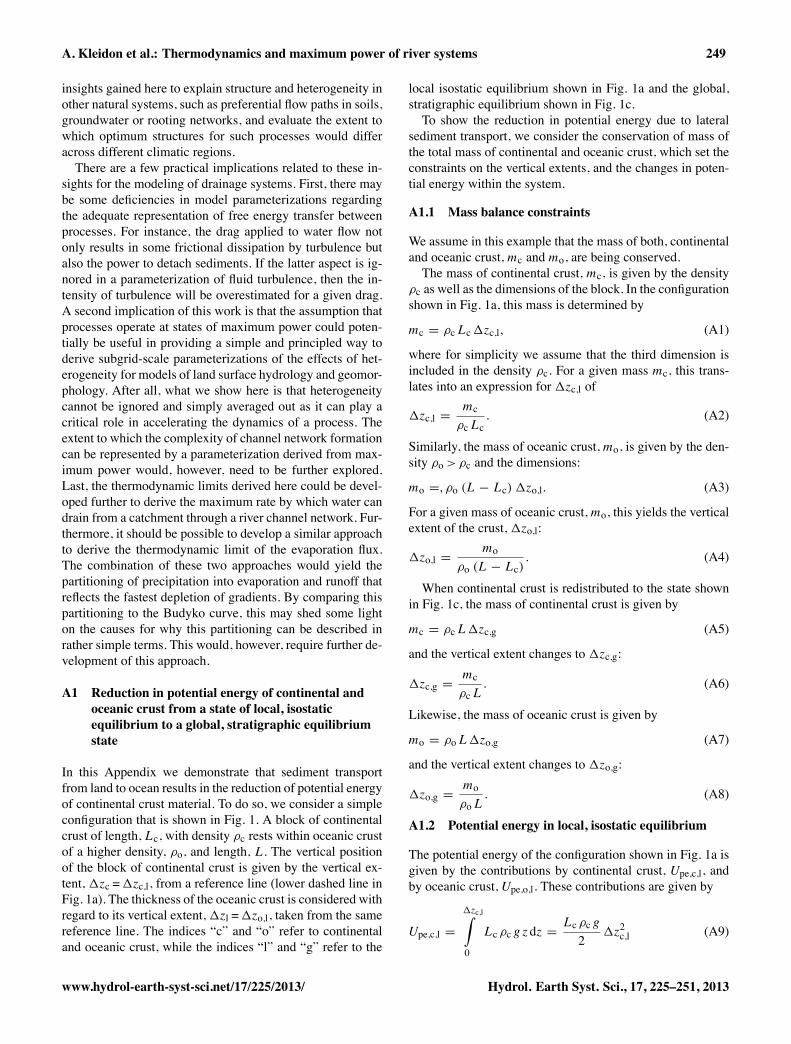
A. Kleidon et al.: Thermodynamics and maximum power of river systems 249
insights gained here to explain structure and heterogeneity inother natural systems, such as preferential flow paths in soils,groundwater or rooting networks, and evaluate the extent towhich optimum structures for such processes would differacross different climatic regions.There are a few practical implications related to these in-
sights for the modeling of drainage systems. First, there maybe some deficiencies in model parameterizations regardingthe adequate representation of free energy transfer betweenprocesses. For instance, the drag applied to water flow notonly results in some frictional dissipation by turbulence butalso the power to detach sediments. If the latter aspect is ig-nored in a parameterization of fluid turbulence, then the in-tensity of turbulence will be overestimated for a given drag.A second implication of this work is that the assumption thatprocesses operate at states of maximum power could poten-tially be useful in providing a simple and principled way toderive subgrid-scale parameterizations of the effects of het-erogeneity for models of land surface hydrology and geomor-phology. After all, what we show here is that heterogeneitycannot be ignored and simply averaged out as it can play acritical role in accelerating the dynamics of a process. Theextent to which the complexity of channel network formationcan be represented by a parameterization derived from max-imum power would, however, need to be further explored.Last, the thermodynamic limits derived here could be devel-oped further to derive the maximum rate by which water candrain from a catchment through a river channel network. Fur-thermore, it should be possible to develop a similar approachto derive the thermodynamic limit of the evaporation flux.The combination of these two approaches would yield thepartitioning of precipitation into evaporation and runoff thatreflects the fastest depletion of gradients. By comparing thispartitioning to the Budyko curve, this may shed some lighton the causes for why this partitioning can be described inrather simple terms. This would, however, require further de-velopment of this approach.
A1 Reduction in potential energy of continental andoceanic crust from a state of local, isostaticequilibrium to a global, stratigraphic equilibriumstate
In this Appendix we demonstrate that sediment transportfrom land to ocean results in the reduction of potential energyof continental crust material. To do so, we consider a simpleconfiguration that is shown in Fig. 1. A block of continentalcrust of length, Lc, with density ρc rests within oceanic crustof a higher density, ρo, and length, L. The vertical positionof the block of continental crust is given by the vertical ex-tent, �zc =�zc,l, from a reference line (lower dashed line inFig. 1a). The thickness of the oceanic crust is considered withregard to its vertical extent,�zl =�zo,l, taken from the samereference line. The indices “c” and “o” refer to continentaland oceanic crust, while the indices “l” and “g” refer to the
local isostatic equilibrium shown in Fig. 1a and the global,stratigraphic equilibrium shown in Fig. 1c.To show the reduction in potential energy due to lateral
sediment transport, we consider the conservation of mass ofthe total mass of continental and oceanic crust, which set theconstraints on the vertical extents, and the changes in poten-tial energy within the system.
A1.1 Mass balance constraints
We assume in this example that the mass of both, continentaland oceanic crust, mc and mo, are being conserved.The mass of continental crust, mc, is given by the density
ρc as well as the dimensions of the block. In the configurationshown in Fig. 1a, this mass is determined by
mc = ρcLc�zc,l, (A1)
where for simplicity we assume that the third dimension isincluded in the density ρc. For a given mass mc, this trans-lates into an expression for �zc,l of
�zc,l = mcρcLc
. (A2)
Similarly, the mass of oceanic crust, mo, is given by the den-sity ρo> ρc and the dimensions:
mo =,ρo (L − Lc) �zo,l. (A3)
For a given mass of oceanic crust, mo, this yields the verticalextent of the crust, �zo,l:
�zo,l = moρo (L − Lc)
. (A4)
When continental crust is redistributed to the state shownin Fig. 1c, the mass of continental crust is given by
mc = ρcL�zc,g (A5)
and the vertical extent changes to �zc,g:
�zc,g = mcρcL
. (A6)
Likewise, the mass of oceanic crust is given by
mo = ρoL�zo,g (A7)
and the vertical extent changes to �zo,g:
�zo,g = moρoL
. (A8)
A1.2 Potential energy in local, isostatic equilibrium
The potential energy of the configuration shown in Fig. 1a isgiven by the contributions by continental crust, Upe,c,l, andby oceanic crust, Upe,o,l. These contributions are given by
Upe,c,l =�zc,l�
0
Lcρc g zdz = Lcρc g
2�z
2c,l (A9)
www.hydrol-earth-syst-sci.net/17/225/2013/ Hydrol. Earth Syst. Sci., 17, 225–251, 2013
250 A. Kleidon et al.: Thermodynamics and maximum power of river systems
and
Upe,o,l =�zo,l�
0
(L − Lc) ρo g zdz = (L − Lc) ρo g
2�z
2o,l. (A10)
Using Eqs. (A2) and (A4) to express �zc,l and �zo,l interms of the masses mc and mo, the total potential energy isexpressed by
Upe,tot,l = Upe,o,l + Upe,c,l = g
2Lcρcm2c + g
2 (L − Lc) ρom2o. (A11)
A1.3 Potential energy in global, stratigraphicequilibrium
The potential energy of the configuration shown in Fig. 1cis derived equivalently. The individual contributions by thecontinental and oceanic crust are given by
Upe,c,g =�zc,g�
0
Lρc g zdz = Lρc g
2
��z
2c,g − �z
2o,g
�(A12)
and
Upe,o,g =�zo,g�
0
Lρo g zdz = Lρo g
2�z
2o,g. (A13)
Taken together, and using Eqs. (A6) and (A8) as above toexpress �zc,g and �zo,g in terms of the masses mc and mo,we obtain
Upe,tot,g = Upe,o,g + Upe,c,g = g
2Lρcm2c + g
2Lρom2o
�1 − ρc
ρo
�. (A14)
A1.4 Difference in potential energy
We now consider the difference in potential energy,�Upe,tot,between the global equilibrium state shown in Fig. 1c to thelocal equilibrium state shown in Fig.1a. We use Eqs. (A11)and (A14) to get the following expression for �Upe,tot:
�Upe,tot = Upe,tot,g − Upe,tot,l = gm2c
2ρc
�1L
− 1Lc
�
+ gm2o
2ρo
�1L
�1 − ρc
ρo
�− 1
L − Lc
�
= − gm2c
2ρcLc
�1 − Lc
L
�
− gm2o
2ρo (L − Lc)
�1 −
�1 − Lc
L
� �1 − ρc
ρo
��. (A15)
What can be seen from Eq. (A15) is that both terms are neg-ative, i.e. that the potential energy decreases from the stateshown in Fig 1a to c.
A1.5 Summary
In summary, this note shows in relatively simple terms thatthe transition from a local isostatic equilibrium to a globalstratigraphic equilibrium is accompanied by a reduction ofpotential energy in the overall system.In principle, one could also show that the initial state of
local isostatic equilibrium represents a state of minimum po-tential energy with respect to the vertical position of con-tinental crust, �zc,j, and that the state of global equilib-rium represents a state of minimum potential energy with re-spect to the horizontal extent of continental crust, Lc. Thiswould, however, require quite lengthly algebraic computa-tions, which has been omitted here for reasons of brevity.
Acknowledgements. We thank one anonymous reviewer, Hu-bert Savenije, Kyungrock Paik, and Greg Tucker for veryconstructive reviews that helped to improve this manuscript.A. K. acknowledges financial support from the Helmholtz Alliance“Planetary Evolution and Life”. This research contributes to the“Catchments As Organized Systems (CAOS)” research groupfunded by the German Science Foundation (DFG).
The service charges for this open access publicationhave been covered by the Max Planck Society.
Edited by: M. Sivapalan
References
Ahnert, F.: Functional relationships between denudation, relief anduplift in large mid-latitude drainage basins, Am. J. Sci., 268,243–263, 1970.
Bagnold, R. A.: An approach to the sediment transport problemfrom general physics, US Geological Survey professional paper422-I, US government printing officce, Washington, DC, USA,1966.
Bejan, A.: Advanced Engineering Thermodynamics, Wiley, NewYork, 1997.
Bejan, A. and Lorente, S.: The constructal law and the evolution ofdesign in nature, Phys. Life Rev., 8, 209–240, 2011.
Dewar, R. C.: Maximum entropy production and the fluctuation the-orem, J. Phys. A, 38, 371–381, 2005.
Dewar, R. C.: Maximum entropy production as an inference algo-rithm that translates physical assumptions into macroscopic pre-dictions: don’t shoot the messenger, Entropy, 11, 931–944, 2010.
Dietrich, W. E. and Perron, J. T.: The search for a topographic sig-nature of life, Nature, 439, 411–418, 2006.
Dyke, J. G., Gans, F., and Kleidon, A.: Towards understandinghow surface life can affect interior geological processes: a non-equilibrium thermodynamics approach, Earth Syst. Dynam., 2,139–160, doi:10.5194/esd-2-139-2011, 2011.
Howard, A. D.: Theoretical model of optimal drainage networks,Water Resour. Res., 26, 2107–2117, 1990.
Izumi, N. and Parker, G.: Linear stability analysis of channel incep-tion: downstream-driven theory, J. Fluid Mech., 419, 239–262,2000.
Hydrol. Earth Syst. Sci., 17, 225–251, 2013 www.hydrol-earth-syst-sci.net/17/225/2013/

A. Kleidon et al.: Thermodynamics and maximum power of river systems 251
Kirkby, M. J.: Hillslope process-response models based on the con-tinuity equation, Inst. Brit. Geogr., Spec. Publ., 3, 15–30, 1971.
Kleidon, A.: Life, hierarchy, and the thermodynamic machinery ofplanet Earth, Phys. Life Rev., 7, 424–460, 2010a.
Kleidon, A.: A basic introduction to the thermodynamics of theEarth system far from equilibrium and maximum entropy pro-duction, Philos. T. Roy. Soc. B, 365, 1303–1315, 2010b.
Kleidon, A.: How does the earth system generate and maintain ther-modynamic disequilibrium and what does it imply for the futureof the planet?, Philos. T. Roy. Soc. A, 370, 1012–1040, 2012.
Kleidon, A. and Schymanski, S. J.: Thermodynamics and optimalityof the water budget on land: a review, Geophys. Res. Lett., 35,L20404, doi:10.1029/2008GL035393, 2008.
Kleidon, A., Malhi, Y., and Cox, P. M.: Maximum entropy pro-duction in environmental and ecological systems, Philos. T. Roy.Soc. B, 365, 1297–1302, 2010.
Kleidon, A., Zehe, E., and Lin, H. S.: Thermodynamic Limits in theCritical Zone and Its Relevance to Hydropedology, in: Hydrope-dology: Synergistic Integration of Soil Science and Hydrology,edited by: Lin, H., Elsevier, Amsterdam, The Netherlands, 243–284, 2012a.
Kleidon, A., Zehe, E., Ehret, U., and Scherer, U.: Interactive Com-ment on “Thermodynamics, maximum power, and the dynamicsof preferential river flow structures on continents” by A. Kleidonet al., Hydrol. Earth Syst. Sci. Discuss., 9, C3466–C3469, 2012b.
Lenton, T. M.: Gaia and natural selection, Nature, 394, 439–447,1998.
Leopold, L. B. and Langbein, W. B.: The concept of entropy in land-scape evolution, US Geol. Surv. Prof. Pap. 500-A, US govern-ment printing office, Washington, DC, USA, 1962.
Lotka, A. J.: Contribution to the energetics of evolution, P. Natl.Acad. Sci. USA, 8, 147–151, 1922a.
Lotka, A. J.: Natural selection as a physical principle, P. Natl. Acad.Sci. USA, 8, 151–154, 1922b.
Odum, E. P.: The strategy of ecosystem development, Science, 164,262–270, 1969.
Odum, H. T.: Self-organization, transformity, and information, Sci-ence, 242, 1132–1139, 1988.
Ozawa, H., Ohmura, A., Lorenz, R. D., and Pujol, T.: The secondlaw of thermodynamics and the global climate system: a reviewof the maximum entropy production principle, Rev. Geophys.,41, 1018, doi:10.1029/2002RG000113, 2003.
Paik, K.: Optimization approach for 4-D natural landscape evolu-tion, IEEE T. Evol. Comput., 15, 684–691, 2011.
Paik, K. and Kumar, P.: Optimality approaches to describe charac-teristic fluvial patterns on landscapes, Philos. T. Roy. Soc. B, 365,1387–1395, 2010.
Paltridge, G. W.: Global dynamics and climate – a system of mini-mum entropy exchange, Q. J. Roy. Meteorol. Soc., 101, 475–484,1975.
Paltridge, G. W.: Climate and thermodynamic systems of maximumdissipation, Nature, 279, 630–631, 1979.
Phillips, J. D.: Biological energy in landscape evolution, Am. J. Sci.,309, 271–289, doi:10.2475/04.2009.01, 2009.
Phillips, J. D.: The job of the river, Earth Surf. Proc. Land., 35,305–313, 2010.
Rinaldo, A., Rodriguez-Iturbe, I., Rigon, R., Bras, R. L., Ijjasz-Vasquez, E., and Marani, A.: Minimum energy and fractal struc-tures of drainage networks, Water Resour. Res., 28, 2183–2195,1992.
Rodriguez-Iturbe, I. and Rinaldo, A.: Fractal River Basins, Chanceand Self-Organization, Cambridge University Press, New York,1997.
Rodriguez-Iturbe, I., Rinaldo, A., Rigon, R., Bras, R. L., Marani,A., and Ijjasz-Vasquez, E.: Energy dissipation, runoff production,and the three-dimensional structure of river basins, Water Resour.Res., 28, 1095–1103, 1992a.
Rodriguez-Iturbe, I., Rinaldo, A., Rigon, R., Bras, R. L., Ijjasz-Vasquez, E., and Marani, A.: Fractal structures as least energypatterns: the case of river networks, Geophys. Res. Lett., 9, 889–892, 1992b.
Smith, T. R.: A theory for the emergence of channelized drainage, J.Geophys. Res., 115, F02023, doi:10.1029/2008JF001114, 2010.
Smith, T. R. and Bretherton, F. P.: Stability and the conservation ofmass in drainage basin evolution, Water Resour. Res., 8, 1506–1529, 1972.
Wang, J. and Bras, R. L.: A model of evapotranspiration based onthe theory of maximum entropy production, Water Resour. Res.,47, W03521, doi:10.1029/2010WR009392, 2011.
West, G. B., Brown, J. H., and Enquist, B. J.: A general model forthe origin of allometric scaling laws in biology, Science, 276,122–126, 1997.
Whipple, K. X. and Tucker, G. E.: Implications of sediment-flux-dependent river incision models for landscape evolution, J. Geo-phys. Res., 107, 2039, doi:10.1029/2000JB000044, 2002.
Woldenberg, M. J.: Spatial order in fluvial systems: Horton’s lawsderived from mixed hexagonal hierarchies of drainage basin ar-eas, Geol. Soc. Am. Bull., 80, 97–112, 1969.
Zehe, E., Blume, T., and Bloschl, G.: The principle of maximumenergy dissipation: a novel thermodynamic perspective on rapidwater flow in connected soil structures, Philos. T. Roy. Soc. B,365, 1377–1386, 2010.
www.hydrol-earth-syst-sci.net/17/225/2013/ Hydrol. Earth Syst. Sci., 17, 225–251, 2013