thermodynamically consistent time-stepping algorithms for non-linear thermomechanical systems

INTERNATIONAL JOURNAL FOR NUMERICAL METHODS IN ENGINEERINGInt. J. Numer. Meth. Engng 2009; 79:706–732Published online 4 March 2009 in Wiley InterScience (www.interscience.wiley.com). DOI: 10.1002/nme.2588

Thermodynamically consistent time-stepping algorithmsfor non-linear thermomechanical systems

Ignacio Romero∗,†

Computational Mechanics Group, E.T.S. Ingenieros Industriales, Universidad Politecnica de Madrid,28006 Madrid, Spain

SUMMARY

We present the basic theory for developing novel monolithic and staggered time-stepping algorithms forgeneral non-linear, coupled, thermomechanical problems. The proposed methods are thermodynamicallyconsistent in the sense that their solutions rigorously comply with the two laws of thermodynamics:for isolated systems they preserve the total energy and the entropy never decreases. Furthermore, ifthe governing equations of the problem have symmetries, the proposed integrators preserve them too.The formulation of such methods is based on two ideas: expressing the evolution equation in the so-called General Equations for Non-Equilibrium Reversible Irreversible Coupling format and enforcing fromtheir inception certain directionality and degeneracy conditions on the discrete vector fields. The newmethods can be considered as an extension of the energy–momentum integration algorithms to coupledthermomechanical problems, to which they reduce in the purely Hamiltonian case. In the article, thenew ideas are applied to a simple coupled problem: a double thermoelastic pendulum with symmetry.Numerical simulations verify the qualitative features of the proposed methods and illustrate their excellentnumerical stability, which stems precisely from their ability to preserve the structure of the evolutionequations they discretize. Copyright q 2009 John Wiley & Sons, Ltd.

Received 10 September 2008; Revised 28 January 2009; Accepted 29 January 2009

KEY WORDS: time integration; structure preservation; geometric integration; coupled problems; thermo-dynamics

1. INTRODUCTION

Structure-preserving integrators, also known as geometric integrators, have had an incrediblesuccess in applied mathematics during the past two decades (see, for example, the monograph [1]).

∗Correspondence to: Ignacio Romero, Dpto. de Mecanica Estructural, E.T.S. Ingenieros Industriales, Jose GutierezAbascal, 2, 28006 Madrid, Spain.

†E-mail: [email protected]

Contract/grant sponsor: Spanish Ministry of Education and Science; contract/grant number: DPI2006-14104

Copyright q 2009 John Wiley & Sons, Ltd.

THERMODYNAMICALLY CONSISTENT TIME-STEPPING ALGORITHMS 707

At the same time, this type of methods has shown a remarkable development in the context ofcomputational mechanics. For example, the energy–momentum algorithm [2–7] has been an activetopic of research from the 1970s until today with many contributions. Another more recent typeof geometric integrators that is an active area of research is the field of variational integrators (see,among many others, [8–11]).

Mainly three reasons explain the success of structure-preserving integrators. First, by design,they capture faithfully the qualitative features of the systems that they try to model, yieldingaccurate insights into the global (qualitative) behavior of the latter. Second, excellent long-termperformance has been reported, which is associated precisely with the structure preservation. Third,as it has been repeatedly demonstrated in the case of energy–momentum integrators, they arenumerically very stable, and that allows them to solve even stiff differential equations with largetime step sizes.

In the context of computational mechanics, geometric integrators have been mainly appliedto conservative (Hamiltonian) problems. This is mainly because these problems possess a richgeometric structure (see, for example, [12]) that is well known and that can guide the developmentof appropriate integration algorithms [13–15]. For non-conservative problems, some of the fewexamples of time-stepping algorithms that preserve the conservation laws of momentum and thedissipative behavior of the continuum equations are References [16–18].

The development of structure-preserving integration algorithms for non-isothermal problemsand other coupled problems in computational mechanics has received scarce attention. Someremarkable exceptions are References [19–22] and more recently References [23, 24]. Apart fromthe complexity of this type of problems, probably the reason that explains the lack of geometricintegrators for them is that the ‘geometry’ of the continuum equations itself has not been asstudied as in the isothermal case. In the latter, the rich Hamiltonian or Poisson structure has beenstudied for many years and complete descriptions are common in the literature (for example, in[25–28]). A common structure underlies all the Hamiltonian problems, and this has simplifiedthe design of geometric integrators because the same ideas employed for the development ofgeometric integrators for a simple model such as a non-linear spring/mass system can be extendedand generalized to non-linear elasticity, rods, shells, etc. See, for example, the methodology ofReferences [13, 29, 30].

A common structure for general thermodynamic systems has been recently proposed in [31, 32].The General Equations for Non-Equilibrium Reversible Irreversible Coupling (GENERIC) frame-work allows one to express the evolution equations of any system in terms of reversible andirreversible operators. The reversible part of GENERIC is a generalization of the Poisson structureof Hamiltonian mechanics, and the irreversible part includes the dissipative structure of the equa-tions in the form of a ‘dissipative bracket’. The GENERIC formalism has been widely applied inthe context of non-equilibrium thermodynamics, fluid mechanics, and recently to some problemsof finite solid mechanics [33, 34].

Starting from the GENERIC formalism, we propose a methodology to construct time-steppingalgorithms that respect the reversible/irreversible structure of the evolution equations. Extendingthe general methodology that exists for the formulation of energy–momentum methods (explainedin detail in [13, 14]), we propose integrators that preserve the symmetries of the system whilecapturing accurately the time evolution of energy and entropy. The advantages of such approach arethe same three identified above for general geometric integrators: qualitative accuracy of the discretedynamics picture, good long-term behavior, and enhanced stability in the numerical integration.

Copyright q 2009 John Wiley & Sons, Ltd. Int. J. Numer. Meth. Engng 2009; 79:706–732DOI: 10.1002/nme

708 I. ROMERO

In this article, we present the ideas of a general methodology for algorithmic design to obtainthermodynamically consistent (TC) integrators. The proposed ideas can be applied to generalcoupled problems, but, for concreteness, we shall apply them to the formulation of integratorsfor a simple non-linear thermomechanical system with symmetry: an isolated double thermoe-lastic pendulum. This example, which is further simplified by considering only its motion ona plane, shows energy conservation (since it is isolated), entropy growth due to heat conduc-tion, and possesses a conserved momentum map, the only non-zero component of the angularmomentum.

The first class of TC algorithms proposed are second-order, monolithic methods that preservethe three qualitative properties of the continuum equations: the numerical solution will conformto the two laws of thermodynamics and the symmetries of the equations will be preserved too.The second type of TC algorithms that are introduced share with the first type the conservationproperties, but the latter is staggered and first-order accurate only. The motivation for the staggeredalgorithms stems directly from the GENERIC formalism, which expresses the thermodynamicevolution equations as a sum of a reversible and an irreversible part. Taking advantage of thisnatural partition, it will be simple to obtain fractional step methods in which each of the stepscomplies with the two laws of thermodynamics and preserves the symmetries in the fully discretesetting. This is related to the fractional step algorithms of Reference [19], but in the currentstudy the form of the split is dictated by the GENERIC formalism and, furthermore, each ofthe steps is built so as to numerically inherit the conservation/dissipation laws of the continuumequations.

The idea of discrete derivative [15] is central for the formulation of the proposed algorithms,but limits their order of accuracy to two. Composition strategies [1, 35] could be employed to raisethe order of accuracy if the methods were symmetric, but the presence of a ‘dissipative bracket’in the problems of interest here spoils this type of symmetry.

Finally, algorithmic numerical damping might be desirable in any time-stepping algorithm. Theideas of References [30, 36] could be incorporated almost directly to the methods developed inthis study, if desired, by modifying appropriately the discrete reversible evolution operator. Bydoing so, the law of energy conservation would be slightly violated (an error proportional tothe order of accuracy of the method), but energy dissipation would always be non-negative and,more importantly, due to the dissipation of unwanted high frequencies of the response. By leavingthe irreversible operators unchanged, the entropy evolution of the modified schemes would bepreserved.

An outline of the rest of the article is as follows. In Section 2 we outline the GENERIC frame-work, restricted to finite-dimensional thermodynamical systems. Next, in Section 3 we proposea general class of time-stepping algorithms that, based on the GENERIC equations, will alwaysconform to the two principles of thermodynamics, and preserve the symmetries of the evolutionequations, if there are any. These integration schemes can be monolithic or staggered, and theyboth share the same preservation properties. To make the ideas more concrete, we describe inSection 4 a relatively simple thermomechanical system with symmetry, and formulate its evolutionequations in the GENERIC form. In Section 5, TC algorithms are proposed for the model problemusing the ideas developed in Section 3. Some numerical simulations obtained with these methodsare presented in Section 6, which confirm the preservation properties of the proposed methods aswell as their remarkable stability and long-term behavior. The article ends with a summary andsome final conclusions in Section 7.



2. A SUMMARY OF THE GENERIC FRAMEWORKFOR FINITE-DIMENSIONAL SYSTEMS

The GENERIC framework is a two-generator formalism that describes the time evolution of generalthermodynamic systems. In this section we review its main features restricted, for simplicity, tofinite-dimensional isolated problems. We refer to the monograph [32] for a complete explanationof the framework, including the infinite-dimensional setting.

To describe the evolution of an isolated thermodynamic system in a time interval I=[0,T ],we consider the state space S whose elements contain all the mechanical, thermal, chemical, etc.variables required to fully represent the system. Denoting time by t ∈I, the state of the systemis a function zt =z(t) :I→S that belongs to C1(0,T ) and whose evolution is described by theinitial value problem

zt =L(zt )∇E(zt )+M(zt )∇S(zt ), z(0)=z0 (1)

where E and S are, respectively, the total energy and entropy of the system, ∇ is the gradientoperator with respect to the state variables z, and L,M are two matrices, possibly depending on z.The notation (·) indicates the time derivative and z0 is the initial state.

The matrix L must be skew-symmetric, whereas M has to be symmetric, positive semidefinite.Moreover, the following two degeneracy conditions must hold:

L(z)∇S(z)=M(z)∇E(z)=0 (2)

Under these conditions, the term associated with the L matrix, the so-called Poisson matrix, is thegenerator of the reversible evolution of the system. Similarly, the term associated with M, denotedas the friction matrix, is responsible for the irreversible part of the system’s evolution.

Expressing the evolution of a system with the formalism (1) has two immediate consequences.Taking the time derivative of the energy, using the skew-symmetry of L and the degeneracyconditions, we obtain

E(z)=∇E(z) · z=∇E(z) ·L(z)∇E(z)+∇E(z) ·M(z)∇S(z)=0 (3)

which expresses the conservation of energy in the isolated system. In a similar manner, taking thetime derivative of the total entropy S it follows that

S(z) = ∇S(z) · z= ∇S(z) ·L(z)∇E(z)+∇S(z) ·M(z)∇S(z)

= ∇S(z) ·M(z)∇S(z)�0 (4)

which is the statement of the second law of thermodynamics for isolated systems.

Remarks 1

1. In some cases, writing the evolution equations of a system in the form (1) serves only toseparate the reversible and irreversible contributions. In other more complex situations, thisframework has allowed to ‘guess’ the form of some of the terms in the equations, and to ruleout functional forms that are intuitively appealing but thermodynamically inconsistent. Thetype of systems we are considering in this article are simple, and their evolution equations


710 I. ROMERO

are well known and thermodynamically sound. However, still, the split (1) will guide us todevelop structure-preserving algorithms.

2. The choice of state variables is, among those that completely describe the system, irrelevantin the sense that if the evolution of the thermodynamical system can be expressed in the form(1) for a given variable z, then for any other complete set b=b(z), the GENERIC evolutionequations can be found by means of a change of variables. However, it is often the casethat the form of the matrices L,M and the gradients ∇E,∇S are much simpler for somechoices of state variables than others. This might be of great advantage for the formulationof time-stepping integration schemes, as will be shown in Section 3.

3. If the thermodynamical system is purely of mechanical nature and conservative, the choicezt =〈q(t),p(t)〉, with q and p being the position and momentum, respectively, results in azero friction matrix M and the Poisson matrix simplifying to

L(z)=[

0 1

−1 0

](5)

which is precisely the canonical symplectic matrix. In this particular situation, the evolutionequations (1) coincide with Hamilton’s equations of motion.

2.1. Symmetries in thermodynamical systems

Symmetries play a key role in the geometric description of Hamiltonian systems, and the same canbe said about more general thermodynamical systems. In the latter context, a symmetry is definedas the action of a (Lie) group on the state space that preserves the reversible and irreversibleoperators. Associated with such actions there are momentum maps that are constant along thesolution if the action preserves both energy and entropy.

In addition, systems with symmetry possess relative equilibria. They are solutions of the evolutionequations, which are also symmetry orbits. A complete description of such actions, as well as theirinfinitesimal generators and the attending momentum maps, is outside the goals of this article.The reader is referred to [28] for the purely Hamiltonian case and to Chapter 6 of [32] for thedefinitions in the GENERIC framework. In Section 3.3 we will address the implications thatsymmetry preservation imposes on TC integrators.

3. ABSTRACT TIME-STEPPING ALGORITHMS FOR GENERALTHERMODYNAMIC SYSTEMS

The design of energy–momentum algorithms for mechanical, conservative problems has benefitedmuch from the common structure that becomes evident when writing the evolution equations in theHamiltonian formalism. Of course, using this framework is not necessary for developing conservingintegrators, but it has made the process simpler, by allowing to identify the key ingredients inthe context of simple problems and then generalizing them to more complex situations. With thesame strategy in mind, we present in this section the basic design ideas that all algorithms forcoupled problems ought to share if they want to inherit the conserving/dissipative structure of thecontinuum equations. It is for this task that writing the equations in the simple form (1) becomesuseful.



To integrate the differential equations (1) in time, the interval [0,T ] is partitioned into N disjointsubintervals In =(tn−1, tn) of length �tn = tn− tn−1 with 0= t0<t1< · · ·<tN =T . At each discretetime tn the value of the state variables will be denoted by zn and thus we seek to approximate thefunction zt by a solution sequence {zn}Nn=0.

3.1. Monolithic integrators

We consider first a monolithic integrator for the complete set of evolution equations (1). We selectit to be of the form

zn+1−zn�tn

=L(zn+1,zn)DE(zn+1,zn)+M(zn+1,zn)DS(zn+1,zn) (6)

In the previous formula, we have replaced the time derivative zt of Equation (1) by its forwarddifferences approximation and the rest of the terms of the GENERIC evolution equation byconsistent approximations to be defined. The discrete operators L,M and the discrete gradientsDE,DS must be, at least, second-order approximation to their continuous counterparts at themidpoint tn+1/2=(tn+ tn+1)/2. The specific form of each of them is dictated by the propertiesthat we would like to enforce in the ensuing method. At this point we only point out that thediscrete operators and gradients are functions of two sets of state variables and they must verifythe consistency properties:

L(zn+1,zn) = L(zn+1/2)+O(�t2n )

M(zn+1,zn) = M(zn+1/2)+O(�t2n )

DE(zn+1,zn) = ∇E(zn+1/2)+O(�t2n )

DS(zn+1,zn) = ∇S(zn+1/2)+O(�t2n )

(7)

where zn+1/2= 12 (zn+zn+1).

The discrete Poisson matrix L is required to be skew-symmetric, and the discrete friction matrixM symmetric and positive semidefinite. As in [13, 14], we require that the discrete gradients DEand DS have the following directionality property:

DE(zn+1,zn) ·(zn+1−zn) = E(zn+1)−E(zn)

DS(zn+1,zn) ·(zn+1−zn) = S(zn+1)−S(zn)(8)

In the same references a specific expression for discrete gradients in Hamiltonian systems is given.For more general systems, such as those into consideration in this study, the formulas are slightlymore involved, as we will show, but the ideas are identical.

Finally, the degeneracy conditions (2) must be replicated by the discrete operators and thus werequire

L(zn,zn+1)DS(zn,zn+1)=M(zn,zn+1)DE(zn,zn+1)=0 (9)

Under the previous conditions we have the fundamental property:

Theorem 1A time-stepping algorithm of the form (6) that verifies (7)–(9) with L skew-symmetric and Msymmetric positive semidefinite has a solution sequence {zn}Nn=1 whose total energy E remainsconstant and whose total entropy S never decreases.


712 I. ROMERO

ProofThe proof follows the same arguments employed in Section 2 to show the conservation of energyand non-decay of entropy. First, to show that the energy is preserved, we start from (8)1 and usethe evolution equation (6):

E(zn+1)−E(zn) = DE(zn+1,zn) ·(zn+1−zn)

= �tnDE(zn+1,zn) ·L(zn+1,zn)DE(zn+1,zn)

+�tnDE(zn+1,zn) ·M(zn+1,zn)DS(zn+1,zn)

= 0 (10)

because of the skew-symmetry of L and the discrete degeneracy condition (9). To prove discretecounterpart of the second law of thermodynamics, we start from the directionality condition (8)2and use the discrete evolution equation (6) as well as the properties of the matrices L and M:

S(zn+1)−S(zn) = DS(zn+1,zn) ·(zn+1−zn)

= �tnDS(zn+1,zn) ·L(zn+1,zn)DE(zn+1,zn)

+�tnDS(zn+1,zn) ·M(zn+1,zn)DS(zn+1,zn)

� 0 (11)

�Remarks 2

1. As explained in Section 2, the choice of state variables is, to a certain extent, irrelevant forthe statement of the initial value problem. For the construction of time-stepping algorithmsthis choice is, however, considerably important. An appropriate choice of state variables cansimplify enormously the formulation and implementation of TC integrators. An unfortunatechoice of variables can have the opposite effect. It might happen that for a bad choice of statevariables the satisfaction of the discrete directionality and/or degeneracy conditions becomesimpossible.

2. As observed in Section 2, for Hamiltonian problems expressed in canonical coordinates,the friction matrix M vanishes and the Poisson matrix reduces to the (constant) symplecticmatrix. The formulation of TC methods greatly simplifies in this case since the degeneracyconditions are automatically satisfied. When the directionality condition is verified by thediscrete gradient DE, the resulting scheme is precisely the energy–momentum method. In thissense, in the same way that GENERIC can be thought of as a generalization of Hamilton’sequations, the TC integrators can be considered as a generalization of energy–momentummethods.

3. Numerical schemes that preserve the two laws of thermodynamics possess a strong stabilitycharacter that makes them very robust. In the context of Hamiltonian mechanics this has beenrepeatedly verified by the energy–momentum method (see, for example, [5]). In the contextof fluids, the importance of verifying the second law has been analyzed, for example, in [37].



3.2. Staggered integrators

The evolution equations (1) naturally suggest a split that can be used to define fractional steptime-stepping methods. The energy gradient, through the Poisson matrix, furnishes a vector fieldthat generates the reversible part of the dynamics. Likewise, the entropy gradient, through thefriction matrix, gives a vector field that generates the irreversible dynamics. A staggered integratorcan be formulated by performing, in each time step, first the numerical integration of the reversiblepart, and later the integration of the irreversible part (or vice versa). The practical usefulness ofsuch a split depends on the choice of state variables but it will be shown next that, in any case, itinherits the structure-preserving properties of its monolithic counterpart.

To define the fractional step method, we consider the same partition of the time integrationinterval [0,T ] as above. Given a solution zn at time tn , the solution zn+1 at the next discrete timeinstant tn+1= tn+�tn is obtained by solving first a reversible step:

zn+1−zn�tn

=L(zn+1,zn)DE(zn+1,zn) (12)

and then an irreversible step:

zn+1− zn+1

�tn=M(zn+1, zn+1)DS(zn+1, zn+1) (13)

The vector zn+1 represents the state of the system after it evolves, reversibly, from the state zn .The staggered method possesses the following property:

Theorem 2The fractional step method (12)–(13), with consistent discrete operators L,M and gradients DE,DSthat satisfy the discrete degeneracy and directionality conditions, yields a solution sequence {zn}Nn=1consistent with the two laws of thermodynamics.

ProofThe reversible step (12) is energy and entropy conserving. To check this, it suffices to repeatthe proof of Theorem 1 for the differences E(zn+1)−E(zn) and S(zn+1)−S(zn). The irreversiblestep (13) is energy conserving but entropy is non-decreasing. To prove this, it suffices again torepeat the same arguments for the differences E(zn+1)−E(zn+1) and S(zn+1)−S(zn+1). Detailsare omitted. �

Remarks 3

1. The staggered method (12)–(13) is only first-order accurate; therefore, the accuracy require-ments for the discrete matrices L,M as well as the discrete gradients DE,DS might berelaxed.

2. A second-order accurate, staggered method can be obtained by using the so-called Strangsplit, which would consist, in this context, of a reversible step of size �tn/2, followed bya irreversible step of size �tn , and finally another reversible step of size �tn/2 (or viceversa). The conservation properties of the ensuing method are also guaranteed by the samearguments as for the first-order method.

3. Staggered schemes that preserve the conservation/dissipation properties of their monolithiccounterparts also share their strong stability. See [19] for a discussion of this and related


714 I. ROMERO

aspects. In Section 5 we will show that the conservation of energy and non-decrease ofentropy imply the non-linear stability of the discrete solution.

4. In [19], the authors prove that in order to obtain fractional step methods with improvedstability, the split of the continuum operator has to be performed in such a way that eachof its parts generates a stable semigroup. The staggered TC methods not only are based onstable operators, but also the discrete advancing maps exactly preserve the stability of thecontinuum equations. This results in further stability gains.

3.3. Integrators for thermodynamical systems with symmetries

As mentioned in Section 2.1, general thermodynamic systems with symmetries possess momentummaps, which are preserved by the flow under certain conditions. If these conditions are met, itwould be desirable that the algorithms employed to integrate the equations also preserve them.

The key ideas to incorporate such desirable properties into the general type of TC algorithmsintroduced in this section can also be found in the literature of energy–momentum methods. Wefollow again Gonzalez [13, 14].

If the state spaceS has dimension n and the orbits of the symmetry group have dimension s thenthere must be n−s invariants of the symmetry denoted by p=(�1,�2, . . . ,�n−s). Let E :p(S)→R

and S :p(S)→R be the reduced energy and entropy, respectively, in a thermodynamical systemwith symmetry defined by

E(p(z))=E(z), S(p(z))= S(z) (14)

Then, extending the ideas of Reference [13], the following definitions of the discrete gradients:

DE(zn+1,zn) = ∇p(zn+1/2)TDE(p(zn+1),p(zn))

DS(zn+1,zn) = ∇p(zn+1/2)TDS(p(zn+1),p(zn))

(15)

will preserve the momentum map, in addition to satisfying the accuracy, directionality, and degen-eracy property. We will show a specific example of such a construction in Section 4.

Time-stepping algorithms that preserve energy and angular momentum have discrete relativeequilibria, that is, solutions that are themselves discrete symmetry orbits. These may or may notlie on the exact relative equilibria. See [38] for an illustration and explicit calculation of a relativeequilibrium in a simple context.

4. A THERMODYNAMIC MODEL PROBLEM

The ideas of Section 3 are applied next to the design of a TC time-stepping algorithm for a modelproblem: an isolated, plane, thermoelastic double pendulum. This simple thermodynamical systempossesses, despite its simplicity, many interesting features and serves to illustrate the constructionof TC integrators and their properties. In particular, in addition to verifying the two laws ofthermodynamics, this is a system with symmetry, and the attendant conservation law should bepreserved by the algorithm too.

The model problem under consideration consists of two point masses m1 and m2 connected bythermoelastic springs of internal energy ea and eb and tied to a fixed point as depicted in Figure 1.The motion of the masses takes place on the plane and their position and momenta are denoted



Figure 1. Model problem: a double thermoelastic pendulum.

as q1,q2 and p1,p2, respectively. The entropies of the springs are denoted, respectively, as sa,sb,and their natural lengths as �0a,�

0b. With this notation, we choose as state variables of the whole

system the vector

z=〈q1,q2,p1,p2,sa,sb〉 (16)

The state space is hence

S={z∈(R2×R2×R2×R2×R+×R+), q1 �=0, q2 �=q1} (17)

and thus has dimension equal to 10. The total energy of the system E can be expressed as thesum of the kinetic energy of the point masses Ki and the internal energy of the springs ei :

E = E(z)=K1(z)+K2(z)+ea(�a,sa)+eb(�b,sb)

Ki (z) = 1

2mi|pi |2 for i=1,2

(18)

The lengths of the springs �a,�b are defined solely in terms of the positions as

�a =√q1 ·q1, �b=√(q2−q1) ·(q2−q1) (19)

The total entropy of the system is obtained as the sum of the entropies of the two springs:

S= S(z)=sa+sb (20)

The model captures the simplest thermal effects: the internal energy should account for the stretchescaused by temperature changes, and the temperature changes due to Gough–Joule effect. Theprecise value of the absolute temperatures �i at each of the springs is obtained through the relations

�a = �ea�sa

, �b= �eb�sb

(21)


716 I. ROMERO

Temperature differences between the two springs cause a heat flux from the hottest to the coldestspring, passing through mass m1, being proportional to the temperature difference and a certainconductivity constant �>0.

The evolution equations of the previous thermodynamic system are

q1 = p1/m1

q2 = p2/m2

p1 = − ��q1

(ea+eb)

p2 = − ��q2

(ea+eb)

sa = �

(�b�a

−1

)

sb = �

(�a�b

−1

)

(22)

The last two equations express the balance of energy in each of the two springs.To restate these equations in the form (1) we start by evaluating the energy and entropy gradients:

∇E(z)=⟨fama− fbmb, fbmb,

p1m1

,p2m2

,�a,�b

⟩, ∇S(z)=〈0,0,0,0,1,1〉 (23)

In the previous expressions, fa, fb,ma,mb are, respectively, the stretching forces and the unitvectors in the directions of the corresponding springs. Using these gradients, Equations (22) canbe expressed in GENERIC form by defining the Poisson and friction matrices to be

L(z)=

⎡⎢⎢⎢⎢⎢⎢⎢⎢⎢⎢⎣

0 0 1 0 0 0

0 0 0 1 0 0

−1 0 0 0 0 0

0 −1 0 0 0 0

0 0 0 0 0 0

0 0 0 0 0 0

⎤⎥⎥⎥⎥⎥⎥⎥⎥⎥⎥⎦

, M(z)=

⎡⎢⎢⎢⎢⎢⎢⎢⎢⎢⎢⎢⎢⎢⎢⎣

0 0 0 0 0 0

0 0 0 0 0 0

0 0 0 0 0 0

0 0 0 0 0 0

0 0 0 0 ��b�a

−�

0 0 0 0 −� ��a�b

⎤⎥⎥⎥⎥⎥⎥⎥⎥⎥⎥⎥⎥⎥⎥⎦

(24)

The simple form of these two matrices will greatly simplify the development of TC algorithmsin Section 5. We remark that, as required, L is skew-symmetric and M is symmetric positivesemidefinite. In the matrix M, the temperature fields, although not indicated, are functions of thestate variables z.

Other choices of state variables are possible. For the energy variables z=〈q1,q2,p1,p2,ea,eb〉,the energy and entropy gradients are

∇E(z)=⟨0,0,

p1m1

,p2m2

,1,1

⟩, ∇S(z)=

⟨fa�ama− fb

�bmb,

fb�bmb,0,0,

1

�a,1

�b

⟩(25)



and the Poisson and friction matrices can be shown to be

L(z) =

⎡⎢⎢⎢⎢⎢⎢⎢⎢⎢⎢⎢⎣

0 0 1 0 0 0

0 0 0 1 0 0

−1 0 0 0 − fama fbmb

0 −1 0 0 0 − fbmb

0 0 famTa 0 0 0

0 0 − fbmTb fbm

Tb 0 0

⎤⎥⎥⎥⎥⎥⎥⎥⎥⎥⎥⎥⎦

M(z) = ��a�b

⎡⎢⎢⎢⎢⎢⎢⎢⎢⎢⎢⎣

0 0 0 0 0 0

0 0 0 0 0 0

0 0 0 0 0 0

0 0 0 0 0 0

0 0 0 0 1 −1

0 0 0 0 −1 1

⎤⎥⎥⎥⎥⎥⎥⎥⎥⎥⎥⎦

(26)

A third choice of state of state variable is ¯z=〈q1,q2,p1,p2,�a,�b〉. This is a very common choicedue to its clear physical meaning. However, the Poisson and friction matrices in this case arevery cumbersome. Even though the continuum GENERIC equations are equivalent, irrespectiveof the choice of state variables, the choice of physical variables would make it very difficult,if not impossible, to construct discrete Poisson and friction matrices that comply with all therequirements identified in Section 2. For this reason we will now pursue the development of a TCintegrator in physical variables.

5. TC INTEGRATORS FOR THE MODEL PROBLEM

We use next the algorithmic design guidelines of Section 4 to formulate TC integrators for themodel problem of Section 4. First, we construct discrete energy and entropy gradients that areconsistent, satisfy the directionality and degeneracy properties, and respect the symmetries ofcontinuum equations. With these gradients we formulate, first, a monolithic, second-order integratorand then a first-order staggered method. We must note that the construction of discrete gradientsfor thermomechanical problems is more involved than in the purely Hamiltonian case. The ideasare, however, identical.

5.1. Discrete gradients

The choice of state variables determines the functional form of the energy, entropy, and evolutionoperators. In order to successfully obtain discrete gradients and evolution matrices that complywith all the desired requirements, we choose to employ entropy variables for the simplicity of theensuing operators.


718 I. ROMERO

To form the discrete gradients, we first identify the invariants of the symmetry within the statespace. The state space has dimension n=10 and the orbits of the symmetry have dimension s=1and we identify, by inspection, the invariants:

�1 = �2a, �2=�2b, �3=|p1|2�4 = |p2|2, �5=sa, �6=sb

�7 = q1 ·p1, �8=q2 ·p2, �9=q1 ·q2(27)

The gradient of the symmetry projection p, required for the definition of the discrete derivatives,can be readily obtained:

∇p(zn+1/2)

=

⎛⎜⎜⎜⎜⎜⎜⎜⎜⎜⎜⎜⎜⎜⎜⎜⎜⎜⎜⎜⎝

2q1,n+1/2 0 0 0 0 0

2(q1,n+1/2−q2,n+1/2) 2(q2,n+1/2−q1,n+1/2) 0 0 0 0

0 0 2p1,n+1/2 0 0 0

0 0 0 2p2,n+1/2 0 0

0 0 0 0 1 0

0 0 0 0 0 1

p1,n+1/2 0 q1,n+1/2 0 0 0

0 p2,n+1/2 0 q2,n+1/2 0 0

q2,n+1/2 q1,n+1/2 0 0 0 0

⎞⎟⎟⎟⎟⎟⎟⎟⎟⎟⎟⎟⎟⎟⎟⎟⎟⎟⎟⎟⎠

(28)

The reduced energy and entropy can be obtained as functions of the reduced variables:

E(zn) = E(pn)= �3,n2m1

+ �4,n2m2

+ea(�1,n,�5,n)+eb(�2,n,�6,n)

S(zn) = S(pn)=�5,n+�6,n

(29)

The reduced discrete energy and entropy gradient can be evaluated by means of (15) together withthe expression (28) and

DE(pn+1,pn) =⟨D�1ea(pn+1,pn),D�2eb(pn+1,pn),

1

2m1,

1

2m2

D�5ea(pn+1,pn),D�6eb(pn+1,pn),0,0,0

⟩TDS(pn+1,pn) = 〈0,0,0,0,1,1,0,0,0〉T

(30)

It remains to define the discrete gradients D�i e j , for i=1,2,5,6 and j =a,b. To guarantee theirdirectionality, they must be constructed according to the rules set forth in [13], carefully accounting



for the multiple arguments of the internal energy functions. These ideas yield

D�i e j (pn+1,pn) = e j (�i,n+1,�i+4,n+1)−e j (�i,n,�i+4,n+1)

2(�i,n+1−�i,n)

+e j (�i,n+1,�i+4,n)−e j (�i,n,�i+4,n)

2(�i,n+1−�i,n), i=1,2 (31)

for the combinations (i, j)=(1,a) and (i, j)=(2,b) and

D�i e j (pn+1,pn) = e j (�i−4,n+1,�i,n+1)−e j (�i−4,n+1,�i,n)

2(�i,n+1−�i,n)

+e j (�i−4,n,�i,n+1)−e j (�i−4,n,�i,n)

2(�i,n+1−�i,n), i=5,6 (32)

for the combinations (i, j)=(5,a) and (i, j)=(6,b). In the limit cases �i,n =�i,n+1, the previousexpressions simplify to their midpoint approximations:

D�i e j (pn+1,pn) = 12 (D1e j (�i,n+1/2,�i+4,n+1)

+D1e j (�i,n+1/2,�i+4,n)), (i, j)=(1,a), (2,b)

D�i e j (pn+1,pn) = 12 (D2e j (�i−4,n+1,�i,n+1/2)

+D2e j (�i−4,n,�i,n+1/2)), (i, j)=(5,a), (6,b)

(33)

where Dk is the standard partial derivative with respect to the kth argument. When i=1,2,the discrete derivative D�i e j is the numerical approximation to the stretching force acting onthe j th spring. Similarly, when i=5,6, the derivative D�i e j is the numerical approximation of thetemperature on the j th spring.

5.2. A monolithic integrator

In addition to the discrete gradients already obtained, to formulate a monolithic integrator as in (6),a discrete Poisson and a friction matrix are required. Only by accuracy considerations, these mustbe of the form

L(zn+1,zn)=L, M(zn+1,zn)=

⎡⎢⎢⎢⎢⎢⎢⎢⎢⎢⎢⎢⎢⎢⎢⎢⎣

0 0 0 0 0 0

0 0 0 0 0 0

0 0 0 0 0 0

0 0 0 0 0 0

0 0 0 0 ��∗b

�∗a

−�

0 0 0 0 −� ��∗a

�∗b

⎤⎥⎥⎥⎥⎥⎥⎥⎥⎥⎥⎥⎥⎥⎥⎥⎦

(34)

where L is the constant Poisson matrix of (24) and �∗a,�

∗b are second-order accurate approxima-

tions to their midpoint counterparts, whose precise form is dictated by the discrete degeneracy


720 I. ROMERO

conditions (9). The degeneracy of L is trivially satisfied due to its simple form and the choice ofstate variables. To verify the degeneracy of the friction matrix M, it suffices to define, for j =a,b,

�∗j (zn+1,zn)=D�i e j (p(zn+1),p(zn)) (35)

with i=5 if j =a and i=6 if j =b. As mentioned above, the discrete derivative of the internalenergy with respect to the entropies �5,�6 yields the algorithmically consistent definitions of thetemperature.

By complying with the guidelines outlined in Section 3, we are certain that the resulting algorithmis TC and preserves the symmetries of the continuum problem. Thus we have the following:

Theorem 3The time-stepping algorithm defined by (6), (30)–(35) is a TC, second-order algorithm for themodel problem that satisfies the two laws of thermodynamics and preserves angular momentum.

5.3. A fractional step integrator

As before, once the discrete gradients and evolution operators are defined, a staggered, TC methodis automatically defined. By construction we also have the following:

Theorem 4The time-stepping algorithm defined by (12)–(13) and the definitions (30)–(35) is a two-step TCalgorithm for the model problem that satisfies the two laws of thermodynamics and that preservesangular momentum. The first step is energy and entropy conserving, and the second step is energyconserving, entropy non-decaying. Both steps preserve the angular momentum.

5.4. Stability

Following the analysis of Reference [19] for the full three-dimensional, finite thermoelasticproblem, we study the appropriate notion of stability for the model problem in its linearized context.In this setting, the double pendulum consists of two linear thermoelastic springs connecting thepoint masses m1, m2 moving on a line parametrized by the real variable x . If we denote by(u1,u2) :I→R2 the displacements of the masses, their momenta by (p1, p2) :I→∈R2, and theirtemperatures increments with respect to a reference temperature �ref by (ϑa,ϑb) :I→∈R2, thethermoelastic problem is contractive in the norm

‖(u1,u2, p1, p2,�a,�b)‖2= p212m1

+ p222m2

+�a(εa,�a)+�b(εb,�b) (36)

where �i =ei −�refsi is the free energy function and εi =�ui/�x , for i=a,b. The free energyfunction must be convex in both arguments so that indeed the function (36) is a true norm on thestate space.

The appropriate notion of stability for the non-linear problem must be analyzed in the extensionof the functional (36) to the non-linear range. With this goal in mind, we define

L(q1,q2,p1,p2,�a,�b)= |p1|22m1

+ |p2|22m2

+�a(�a,�a)+�b(�b,�b) (37)



where �i is, as before, the canonical free energy in the non-linear problem �i =ei −�refsi , fori=a,b. The continuous non-linear thermoelastic problem has then the following stability property:

Theorem 5The solution zt of the double thermoelastic pendulum described in Section 4 satisfies

d

dtL(zt )�0 (38)

ProofBy using the Legendre transform and the definitions of total energy (18) and entropy (20), werewrite

L=K1+K2+ea−�refsa+eb−�refsb=(K1+K2+ea+eb)−�ref(sa+sb) (39)

which means that the functional L can be expressed equivalently as L=E−�refS. Then, theevolution of L along the solution zt is

d

dtL(zt )= d

dtE(zt )−�ref

d

dtS(zt ) (40)

which is non-positive, since energy is preserved, the reference temperature is positive, and entropyhas non-negative time derivative. �

Naturally, time-stepping algorithms whose discrete solution inherit the stability inequality (38)are very robust. We now show that, by construction, all TC algorithms possess such desirableproperty, satisfying the discrete counterpart of Theorem 5.

Theorem 6The monolithic and staggered TC algorithms satisfy the discrete stability property

L(zn+1)�L(zn) (41)

ProofThe same proof as in Theorem 5 can be used, by replacing time derivatives by differences betweensuccessive instants of the discrete solution, since energy is unconditionally preserved by all typesof TC algorithms and entropy never decreases. �

6. NUMERICAL SIMULATIONS

In this section we show three simulations that serve to illustrate the major features of the TCintegrators proposed in Section 5.

6.1. Short-term simulation

In this first example we consider the model problem of Section 4 with the following data: m1=1,m2=2, Ca =0.1, Cb=1, �0a =2, �0b=1, �=300. The free energy of the i th spring takes thenon-linear expression

�i = �(�i ,�i )= Ci

2log2

�i

�0i−�(�i −�ref) log

�i

�0i+c0

(�i −�ref−�i log

�i�ref

)(42)


722 I. ROMERO

for i=a,b, where �ref=300 is the reference temperature, �=0.2 is the coupling parameter, andc0=5 is the heat capacity. The internal energy of each spring, obtained from the partial Legendretransform of the corresponding free energy, is

ei = e(�i ,si )= Ci

2log2

�i

�0i+��ref log

�i

�0i+c0�ref

(exp

(si −� log(�i/�

0i )

co

)−1

)(43)

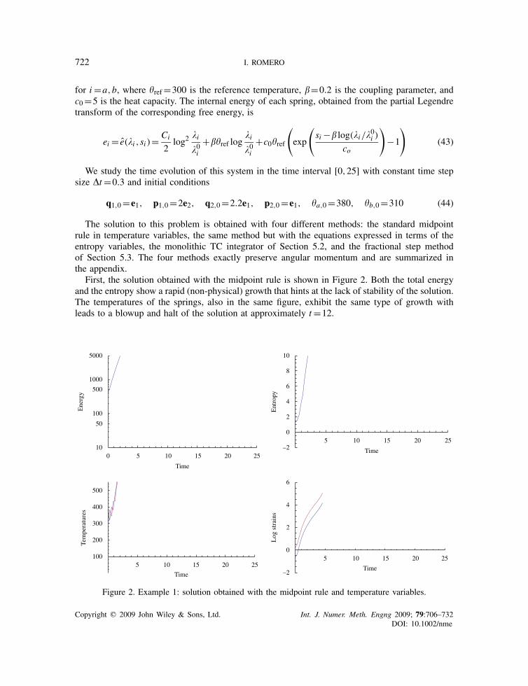
We study the time evolution of this system in the time interval [0,25] with constant time stepsize �t=0.3 and initial conditions

q1,0=e1, p1,0=2e2, q2,0=2.2e1, p2,0=e1, �a,0=380, �b,0=310 (44)

The solution to this problem is obtained with four different methods: the standard midpointrule in temperature variables, the same method but with the equations expressed in terms of theentropy variables, the monolithic TC integrator of Section 5.2, and the fractional step methodof Section 5.3. The four methods exactly preserve angular momentum and are summarized inthe appendix.

First, the solution obtained with the midpoint rule is shown in Figure 2. Both the total energyand the entropy show a rapid (non-physical) growth that hints at the lack of stability of the solution.The temperatures of the springs, also in the same figure, exhibit the same type of growth withleads to a blowup and halt of the solution at approximately t=12.

0 5 10 15 20 25

Time

10

50

100

500

1000

5000

Ene

rgy

5 10 15 20 25

Time–2

0

2

4

6

8

10

Ent

ropy

5 10 15 20 25

Time

100

200

300

400

500

Tem

pera

ture

s

5 10 15 20 25

Time–2

0

2

4

6

Log

str

ains

Figure 2. Example 1: solution obtained with the midpoint rule and temperature variables.



0 5 10 15 20 25

Time

10

50

100

500

1000

5000

Ene

rgy

5 10 15 20 25

Time–2

0

2

4

6

8

10

Ent

ropy

5 10 15 20 25

Time

100

200

300

400

500

Tem

pera

ture

s

5 10 15 20 25

Time–2

0

2

4

6

Log

str

ains

Figure 3. Example 1: solution obtained with the midpoint rule using entropy variables.

0 5 10 15 20 25

Time

10

50

100

500

1000

5000

Ene

rgy

0 5 10 15 20 25

Time

1.00

1.05

1.10

1.15

1.20

1.25

1.30

Ent

ropy

5 10 15 20 25

Time

100

200

300

400

500

Tem

pera

ture

s

5 10 15 20 25

Time–2

0

2

4

6

Log

str

ains

Figure 4. Example 1: solution obtained with the proposed monolithic TC algorithm.


724 I. ROMERO

The solution to the same model problem, using again the midpoint rule, but with the evolutionequations written in entropy variables is depicted in Figure 3. This simple change of variablesresults in a remarkable stability gain. This second method is able to integrate the solution in thewhole time interval although again the solution shows a non-physical evolution of the total energyand entropy. Both quantities oscillate, violating the two laws of thermodynamics. The lack ofcontrol on the energy and entropy is a manifestation of the possible loss of stability, which can beobserved when choosing larger time step sizes. For example, when �t=0.5, this implementationfails to converge after five time steps.

When the monolithic and staggered TC algorithms are employed, the discrete solutions showenergy and entropy evolutions depicted in Figures 4 and 5, respectively. In both cases the energyis perfectly preserved and entropy only grows (note the change of scale in the entropy plot in theselast two figures as compared with the first two). In addition, the algorithms are able to integratethe evolution equations with larger time steps than in the case of the midpoint rule methods. Timestep sizes of over �t=2 can be employed with the data of this example.

6.2. Long-term simulation and relative equilibria

In the second example, the same model problem as before is solved, now with initial data

q1,0=12e1, p1,0=2e2, q2,0=2.2e1, p2,0=e1−2e2, �a,0=290, �b,0=442 (45)

This example serves to illustrate first that, even when stable, a method that is not TC will lead tosolutions that are qualitatively wrong. Second, we want to show that the limit solution obtainedby the TC integrators, if the problem has a symmetry, is a relative equilibrium.

The solution is calculated with the same four methods as before, for a time interval [0,500]and with constant step size �t=0.3. As in the previous example, the standard midpoint ruleapplied to the evolution equations written in temperature variables fails to converge after28 computation steps. The other three methods are able to compute the whole solution. AsFigure 6 shows, the solution obtained with the midpoint rule applied to the evolution equa-tions written in entropy form gives an energy and entropy picture that is completely wrong.Temperature quickly drops to negligible values (close to absolute zero). Both energy and entropydecrease.

In contrast, both the monolithic and staggered TC methods provided almost identical solu-tions, which, furthermore, comply at every instant with the two principles of thermodynamics(Figures 7 and 8) . As before, the three solutions exactly preserve the angular momentum to its initialvalue.

If we compute the solution to this problem with either TC method up to time 1500, thesolution has the features depicted in Figure 9. In the long term, the solution obtained is amotion with constant energy and angular momentum. Moreover, we observe that the entropy,the temperatures, and the strains converge to asymptotic values. In this motion, the spring/masses rotate deformed but with constant stretches in a circular motion with constant angularvelocity and uniform temperature. This type of motion is a relative equilibrium for the problemat hand.

Having relative equilibria as limit sets is a desirable property for time-stepping methods thatintegrate dissipative equations with symmetry. See, for example, [18, 30].



0 5 10 15 20 25

Time

10

50

100

500

1000

5000E

nerg

y

0 5 10 15 20 25

Time

1.00

1.05

1.10

1.15

1.20

1.25

1.30

Ent

ropy

5 10 15 20 25

Time

100

200

300

400

500

Tem

pera

ture

s

5 10 15 20 25

Time–2

0

2

4

6

Log

str

ains

Figure 5. Example 1: solution obtained with the proposed staggered TC algorithm.

0 100 200 300 400 500

Time

10

20

50

100

200

500

1000

2000

Ene

rgy 100 200 300 400 500

Time

–10

–5

0

Ent

ropy

0 100 200 300 400 500

Time

0

100

200

300

400

500

600

Tem

pera

ture

s

100 200 300 400 500

Time

0

2

4

6

8

Log

str

ains

Figure 6. Example 2: solution obtained with the midpoint rule using entropy variables.


726 I. ROMERO

0 100 200 300 400 500

Time

10

20

50

100

200

500

1000

2000E

nerg

y 100 200 300 400

Time

500

–10

–5

0

Ent

ropy

0 100 200 300 400 500

Time

0

100

200

300

400

500

600

Tem

pera

ture

s

100 200 300 400 500

Time

0

2

4

6

8

Log

str

ains

Figure 7. Example 2: solution obtained with the proposed monolithic TC algorithm.

0 100 200 300 400 500

Time

10

20

50

100

200

500

1000

2000

Ene

rgy 100 200 300 400 500

Time

–10

–5

0

Ent

ropy

0 100 200 300 400 500

Time

0

100

200

300

400

500

600

Tem

pera

ture

s

100 200 300 400 500

Time

0

2

4

6

8

Log

str

ains

Figure 8. Example 2: solution obtained with the proposed staggered TC algorithm.



0 200 400 600 800 1000 1200 1400

Time

100

1000

500

200

300

150

700

Ene

rgy

Ene

rgy

0 200 400 600 800 1000 1200 1400

Time

0.0

0.5

1.0

1.5

2.0

2.5

3.0

0 200 400 600 800 1000 1200 1400

Time

200

250

300

350

400

Tem

pera

ture

s

200 400 600 800 1000 1200 1400

Time

0

2

4

6

8

10

Log

str

ains

Figure 9. Example 2: long-term solution obtained with the monolithic TC algorithm.

7. SUMMARY AND CONCLUSIONS

In this article we have proposed a general theory of TC time-stepping integrators for a fairly generalclass of evolution equations in thermomechanics. Such methods integrate in time these equations,providing discrete solutions that satisfy the two laws of thermodynamics and, furthermore, respectthe symmetries of the continuum equations.

The idea for our developments is to start from the GENERIC framework, a formalism that setsthe evolution equations of general thermodynamical systems in a simple and general form thatclearly identifies the reversible and irreversible parts of the dynamics. From this point of departure,and using many of the ideas of energy–momentum integrators, we have been able to set up aseries of requirements that, if satisfied by an integrator, will yield by construction a TC discretesolution.

The choice of state variables for the thermodynamical system is shown to be crucial for thealgorithmic design. Whereas in the continuum setting all state variables are equal, there are certainchoices that can make the formulation of TC algorithms much simpler.

For isolated systems, both the preservation of energy and non-decrease of entropy have beenshown to be crucial for the stability of the algorithms. In fact, energy conservation by itself doesnot provide the appropriate stability notion except for the purely Hamiltonian case. The suitablestability estimates in the continuum and discrete setting have been shown to be a consequence ofthe verification, at both levels, of the two laws of thermodynamics.


728 I. ROMERO

We have discussed these issues in a general finite-dimensional setting and then applied them toa simple thermomechanical problem with symmetry: a double thermoelastic pendulum moving ona plane. The simplicity of the model allows to work out all the specific details and construct, stepby step, the integrator. For this problem we have been able to formulate a second-order monolithicTC scheme and a first-order staggered scheme. The ideas, however, are general enough that canbe applied to any finite-dimensional thermodynamical system, as long as it can be expressed inthe GENERIC form.

The numerical examples presented verify that the proposed algorithms generate discrete solutionsthat comply with the principles of thermodynamics, preserve the symmetries of the problem, andfurthermore are extremely robust and stable when compared with standard implementations.

We are currently working on the extension of the ideas presented in this article to morecomplicated systems in thermomechanics and, in particular, to infinite-dimensional problems. Theextensions need to take care of the difficulties associated with field formulations and more complexsymmetries. For all these cases, the basic ideas of the corresponding TC integrators are those inthe current article, which have to be generalized or adapted.

APPENDIX A

In Section 6 we compared the numerical performance of four integration algorithms for the coupledsolution of the thermoelastic double pendulum. The expressions for the monolithic and staggeredTC algorithms were presented in the text. We summarize the update map for the proposed algorithmsand we provide, for completeness, the expressions of the standard midpoint rule in entropy andtemperature variables, respectively.

A.1. TC algorithms

Given the state of the system at time tn completely described by the state variable zn =(q1,q2,p1,p2,sa,sb), the solution zn+1 at time tn+1= tn+�t is obtained by solving the non-linearsystem of equations

q1,n+1−q1,n�t

= 1

m1p1,n+1/2

q2,n+1−q2,n�t

= 1

m2p2,n+1/2

p1,n+1−p1,n�t

= −2D�1 ea(pn+1,pn)q1,n+1/2−2D�1 eb(pn+1,pn)(q1,n+1/2−q2,n+1/2)

p2,n+1−p2,n�t

= −2D�2 eb(pn+1,pn)(q2,n+1/2−q1,n+1/2)

sa,n+1−sa,n

�t= �

(�∗b

�∗a−1

)

sb,n+1−sb,n�t

= �

(�∗a

�∗b−1

)

(A1)



together with the definitions (31), (32), and (35). The updates employed in each of the steps ofthe staggered TC method are identical to those above.

A.2. Midpoint rule in entropy variables

As before, given the state of the thermoelastic spring at time tn described by the state variablezn =(q1,q2,p1,p2,sa,sb), the solution zn+1 at time tn+1= tn+�t is obtained by solving thenon-linear equations

q1,n+1−q1,n�t

= 1

m1p1,n+1/2

q2,n+1−q2,n�t

= 1

m2p2,n+1/2

p1,n+1−p1,n�t

= −�ea��

(�a,n+1/2,sa,n+1/2)q1,n+1/2

�a,n+1/2

−�eb��

(�b,n+1/2,sb,n+1/2)q1,n+1/2−q2,n+1/2

�b,n+1/2

p2,n+1−p2,n�t

= −�eb��

(�b,n+1/2,sb,n+1/2)q2,n+1/2−q1,n+1/2

�b,n+1/2

sa,n+1−sa,n

�t= �

(�b,n+1/2

�a,n+1/2−1

)

sb,n+1−sb,n�t

= �

(�a,n+1/2

�b,n+1/2−1

)

(A2)

where (·)n+1/2= 12 (·)n+ 1

2 (·)n+1 except for the following terms:

�a,n+1/2 = |q1,n+1/2|�b,n+1/2 = |q2,n+1/2−q1,n+1/2|

�a,n+1/2 = �ea�s

(�a,n+1/2,sa,n+1/2)

�b,n+1/2 = �eb�s

(�b,n+1/2,sb,n+1/2)

(A3)

A.3. Midpoint rule in temperature variables

In contrast with the methods above, the thermomechanical state of the thermoelastic pendulum isdescribed in this method in terms of the temperatures, by means of the free energy. If the stateat time tn is given by the new state variable ¯zn =(q1,q2,p1,p2,�a,�b), the solution ¯zn+1 at time


730 I. ROMERO

tn+1= tn+�t is obtained by solving the non-linear equations

q1,n+1−q1,n�t

= 1

m1p1,n+1/2

q2,n+1−q2,n�t

= 1

m2p2,n+1/2

p1,n+1−p1,n�t

= −��a

��(�a,n+1/2,�a,n+1/2)

q1,n+1/2

�a,n+1/2

−��b

��(�b,n+1/2,�b,n+1/2)

q1,n+1/2−q2,n+1/2

�b,n+1/2

p2,n+1−p2,n�t

= −��b

��(�b,n+1/2,�b,n+1/2)

q2,n+1/2−q1,n+1/2

�b,n+1/2

sa,n+1−sa,n

�t= �

(�b,n+1/2

�a,n+1/2−1

)sb,n+1−sb,n

�t= �

(�a,n+1/2

�b,n+1/2−1

)

(A4)

where, as before, the midpoint notation is defined as (·)n+1/2= 12 (·)n+ 1

2 (·)n+1 except for thefollowing terms:

�a,n+1/2 = |q1,n+1/2|�b,n+1/2 = |q2,n+1/2−q1,n+1/2|

sa,n+1/2 = −��a

��(�a,n+1/2,�a,n+1/2)

sb,n+1/2 = −��b

��(�b,n+1/2,�b,n+1/2)

(A5)

ACKNOWLEDGEMENTS

The author would like to thank Prof. M. Laso of the E.T.S.I. Industriales for many helpful discussionsabout GENERIC and thermodynamics in general. The financial support for this work has been providedby the grant DPI2006-14104 from the Spanish Ministry of Education and Science.

REFERENCES

1. Hairer E, Lubich C, Wanner G. Geometric Numerical Integration. Springer Series in Computational Mathematics.Springer: Berlin, 2002.

2. Labudde RA, Greenspan D. Energy and momentum conserving methods of arbitrary order for the numericalintegration of equations of motion—i. Motion of a single particle. Numerische Mathematik 1976; 25:323–346.

3. Labudde RA, Greenspan D. Energy and momentum conserving methods of arbitrary order for the numericalintegration of equations of motion—ii. Motion of a system of particles. Numerische Mathematik 1976; 25:323–346.

4. Simo JC, Tarnow N, Wong KK. Exact energy–momentum conserving algorithms and symplectic schemes fornonlinear dynamics. Computer Methods in Applied Mechanics and Engineering 1992; 100(1):63–116.



5. Simo JC, Tarnow N. The discrete energy–momentum method. Conserving algorithms for nonlinear elastodynamics.Journal of Applied Mathematics and Physics 1992; 43(5):757–792.

6. Simo JC, Tarnow N, Doblare M. Non-linear dynamics of three-dimensional rods: exact energy and momentumconserving algorithms. International Journal for Numerical Methods in Engineering 1995; 38(9):1431–1473.

7. Simo JC, Tarnow N. A new energy and momentum conserving algorithm for the non-linear dynamics of shells.International Journal for Numerical Methods in Engineering 1994; 37(15):2527–2549.

8. Kane C, Marsden JE, Ortiz M. Symplectic-energy–momentum preserving variational integrators. Preprint, 1999.9. Lew A, Marsden JE, Ortiz M, West M. Variational time integrators. International Journal for Numerical Methods

in Engineering 2004; 60:153–212.10. Marsden JE, West M. Discrete mechanics and variational integrators. Acta Numerica 2001; 10:357–514.11. Wendlandt JM, Marsden JE. Mechanical integrators derived from a discrete variational principle. Physica D

1997; 106(3–4):223–246.12. Simo JC, Marsden JE, Krishnaprasad PS. The Hamiltonian structure of nonlinear elasticity: the material and

convective representations of solids, rods, and plates. Archive for Rational Mechanics and Analysis 1988;104(2):125–183.

13. Gonzalez O. Design and analysis of conserving integrators for nonlinear Hamiltonian systems with symmetry.Ph.D. Thesis, Department of Mechanical Engineering, Stanford University, 1996.

14. Gonzalez O. Time integration and discrete Hamiltonian systems. Journal of Nonlinear Science 1996; 6:449–467.15. Gonzalez O. Exact energy–momentum conserving algorithms for general models in nonlinear elasticity. Computer

Methods in Applied Mechanics and Engineering 2000; 190:1763–1783.16. Armero F, Petocz E. A new dissipative time-stepping algorithm for frictional contact problems: formulation and

analysis. Computer Methods in Applied Mechanics and Engineering 1999; 179:151–178.17. Meng XN, Laursen TA. Energy consistent algorithms for dynamic finite deformation plasticity. Computer Methods

in Applied Mechanics and Engineering 2002; 191:1639–1675.18. Armero F, Zambrana-Rojas C. Volume-preserving energy–momentum schemes for isochoric multiplicative

plasticity. Computer Methods in Applied Mechanics and Engineering 2007; 196:4130–4159.19. Armero F, Simo JC. A new unconditionally stable fractional step method for nonlinear coupled thermomechanical

problems. International Journal for Numerical Methods in Engineering 1992; 35(4):737–766.20. Armero F, Simo JC. Long-term dissipativity of time-stepping algorithms for an abstract evolution equation with

applications to the incompressible MHD and Navier–Stokes equations. Computer Methods in Applied Mechanicsand Engineering 1996; 131(1–2):41–90.

21. Simo JC, Armero F, Taylor CA. Stable and time-dissipative finite element methods for the incompressible Navier–Stokes equations in advection dominated flows. International Journal for Numerical Methods in Engineering1995; 38(9):1475–1506.

22. Simo JC, Armero F. Unconditional stability and long-term behavior of transient algorithms for the incompressibleNavier–Stokes and Euler equations. Computer Methods in Applied Mechanics and Engineering 1994;111(1–2):111–154.

23. Gross M, Betsch P. An energy consistent hybrid space–time Galerkin method for nonlinear thermomechanicalproblems. Proceedings in Applied Mathematics and Mechanics (PAMM), Berlin, vol. 6, 2006; 443–444.

24. Gross M, Betsch P. An energy consistent hybrid space–time finite element method for nonlinear thermo-viscoelastodynamics. In Computational Methods for Coupled Problems in Science and Engineering II,Papadrakakis M, Onate E, Schrefler B (eds). CIMNE: Barcelona, Spain, 2007; 413–416.

25. Abraham RS, Marsden JE. Foundations of Mechanics (2nd edn). Addison-Wesley: Reading, MA, 1978.26. Arnold VI. Mathematical Methods of Classical Mechanics. Springer: Berlin, 1989.27. Arnold VI, Kozlov VV, Neishtadt AI. Mathematical Aspects of Classical and Celestial Mechanics (2nd edn).

Springer: Berlin, 1997.28. Marsden JE, Ratiu TS. Introduction to Mechanics and Symmetry (1st edn). Springer: New York, 1994.29. Tarnow N. Energy and momentum conserving algorithms for hamiltonian systems in the nonlinear dynamics of

solids. Ph.D. Thesis, Stanford University, 1993.30. Armero F, Romero I. On the formulation of high-frequency dissipative time-stepping algorithms for nonlinear

dynamics. Part I: low order methods for two model problems and nonlinear elastodynamics. Computer Methodsin Applied Mechanics and Engineering 2001; 190:2603–2649.

31. Grmela M, Ottinger HC. Dynamics and thermodynamics of complex fluids. I. Development of a general formalism.Physical Review E 1997; 56(6):6620–6632.

32. Ottinger HC. Beyond Equilibrium Thermodynamics. Wiley: New York, 2005.


732 I. ROMERO

33. Hutter M, Tervoort TA. Finite anisotropic elasticity and material frame indifference from a nonequilibriumthermodynamics perspective. Journal of Non-Newtonian Fluid Mechanics 2007; 152:45–52.

34. Hutter M, Tervoort TA. Thermodynamic considerations on nonisothermal finite anisotropic elasto-viscoplasticity.Journal of Non-Newtonian Fluid Mechanics 2007; 152:53–65.

35. Tarnow N, Simo JC. How to render second order accurate time-stepping algorithms fourth order accurate whileretaining the stability and conservation properties. Computer Methods in Applied Mechanics and Engineering1994; 115(3–4):233–252.

36. Armero F, Romero I. On the formulation of high-frequency dissipative time-stepping algorithms for nonlineardynamics. Part II: second order methods. Computer Methods in Applied Mechanics and Engineering 2001;190:6783–6824.

37. Hughes TJR, Franca LP, Mallet M. A new finite element formulation for computational fluid mechanics:I. Symmetric forms of the compressible Euler and Navier–Stokes equations and the second law of thermodynamics.Computer Methods in Applied Mechanics and Engineering 1986; 54:223–234.

38. Gonzalez O, Simo JC. On the stability of symplectic and energy–momentum algorithms for non-linearHamiltonian systems with symmetry. Computer Methods in Applied Mechanics and Engineering 1996; 134(3–4):197–222.


thermodynamically consistent time-stepping algorithms for non-linear thermomechanical systems

Documents