thermo-mechanical modelling of wire-arc additive
TRANSCRIPT

metals
Article
Thermo-Mechanical Modelling of Wire-Arc AdditiveManufacturing (WAAM) of Semi-Finished Products
Marcel Graf 1,*, Andre Hälsig 2, Kevin Höfer 2, Birgit Awiszus 1 and Peter Mayr 2
1 Institute for Machine Tools and Production Processes, Professorship Virtual Production Engineering,Chemnitz University of Technology, Reichenhainer Str. 70, 09126 Chemnitz, Germany;[email protected]
2 Institute of Joining and Assembly, Professorship Welding Engineering, Chemnitz University of Technology,Reichenhainer Str. 70, 09126 Chemnitz, Germany; [email protected] (A.H.);[email protected] (K.H.); [email protected] (P.M.)
* Correspondence: [email protected]; Tel./Fax: +49-371-531-31796
Received: 23 October 2018; Accepted: 24 November 2018; Published: 1 December 2018�����������������
Abstract: Additive manufacturing processes have been investigated for some years, and arecommonly used industrially in the field of plastics for small- and medium-sized series. The use ofmetallic deposition material has been intensively studied on the laboratory scale, but the numericalprediction is not yet state of the art. This paper examines numerical approaches for predictingtemperature fields, distortions, and mechanical properties using the Finite Element (FE) softwareMSC Marc. For process mapping, the filler materials G4Si1 (1.5130) for steel, and AZ31 formagnesium, were first characterized in terms of thermo-physical and thermo-mechanical propertieswith process-relevant cast microstructure. These material parameters are necessary for a detailedthermo-mechanical coupled Finite Element Method (FEM). The focus of the investigations was on thenumerical analysis of the influence of the wire feed (2.5–5.0 m/min) and the weld path orientation(unidirectional or continuous) on the temperature evolution for multi-layered walls of miscellaneousmaterials. For the calibration of the numerical model, the real welding experiments were carriedout using the gas-metal arc-welding process—cold metal transfer (CMT) technology. A uniformwall geometry can be produced with a continuous welding path, because a more homogeneoustemperature distribution results.
Keywords: wire arc additive manufacturing (WAAM); multi-pass welding; FEA; MSC Marc; steelG4Si1; magnesium AZ31
1. Introduction
Additive manufacturing processes have become very significant in recent years. They have manyadvantages in comparison to conventional processes. The production of complex and individualcomponents is possible with additive manufacturing processes. In principle, the layer by layertechnology can use metals to produce almost any profile. The processes generate components by thejoining of meltable materials, where the geometry is continuously built [1]. Additive manufacturingprocesses can also be classified by EN ISO17296-2-2015 into initial material, workpiece size, or energysource [2]. In addition, metallic additive manufacturing processes are subdivided into powder-bed,powder-feed, and wire-feed systems [3,4].
Compared to the powder-bed system, wire-based additive manufacturing processes have a higherdeposition rate, use cheaper filler materials, and require lower investment [5]. Additionally, the wire-arcadditive manufacturing (WAAM) process, in combination with a robot, also allows the productionof complex geometries [6–8]. A component manufactured by a wire-based additive manufacturing
Metals 2018, 8, 1009; doi:10.3390/met8121009 www.mdpi.com/journal/metals

Metals 2018, 8, 1009 2 of 10
technique can achieve the tensile strength of a forged or cast complex component [6]. However,the surface finish and accuracy is poorer than with powder-bed or beam-melting additivetechnologies [9]. In order to produce a high-quality product, it is important to determine theinteraction of each process parameter with the component properties (microstructure, residual stresses),and to combine the process with other production technologies, if necessary [10]. An initial estimatecan be made using numerical methods that take different boundary conditions into consideration.The current aim of the numerical simulation of additive manufacturing processes is the modelling of athermo-mechanical coupled simulation without microstructural properties at mesoscopic level. Variousnumerical methods can be applied for this. On the one hand, the volume-of-fluid method is usedfor the geometrical prediction—to consider the flow behaviour of the molten wire as a drop, and tomodel its solidification and wetting behaviour to the nearest drop [3]. On the other hand, additivetechnologies, such as WAAM or wire laser metal deposition (LMD-W), can also be modelled by a FiniteElement (FE) method based on the element-birth technique, for the determination of real temperaturefields and residual stresses. The focus for this simulation of the WAAM process has been on calculatingtemperature distribution, displacement of components and residual stresses [11–16]. The focus of thispaper is not on powder-bed methods.
2. FE Model
2.1. Material Data
For a transient thermo-mechanical simulation of the multi-layer welding process, it is essentialthat the thermo-physical properties of the filler material be determined, taking the real microstructure(dendritic microstructure) into consideration, and modelled as a function of the temperature(see Figure 1) in addition to the real chemical composition. For the investigated filler materialsAZ31 (magnesium alloy) and G4Si1 (steel alloy), the necessary material data were partly takenfrom the literature [17] and partly calculated in the JMatPro material simulation software Version10 (Sente Software Ltd., Guildford, United Kingdom), or identified by experiments. The materialsoftware JMatPro uses thermo-physical and thermo-dynamic correlations and calculations for thedetermination of material properties in the material equilibria, under consideration of the chemicalcomposition [18]. It should be noted that the samples for the physical simulation were erodedfrom a welding seam, so a comparable microstructural state to the WAAM process was used inthe characterisation. The physical simulation of the thermal expansion coefficient was determinedin the quenching and forming dilatometer Bähr DIL 805 A/T (Bähr Thermoanalyse GmbH nowTA Instruments, Hüllhorst, Germany). The specific heat capacities were measured by differentialscanning calorimetry. For the characterisation of magnesium and G4Si1, the DSC-60 from MettlerToledo (Mettler-Toledo International Inc., Columbus, OH, USA). and the Multi HTC96 from Setaram(SETARAM Instrumentation, Caluire, France). were used respectively. The experimental data representthe average of three measurements.
In the case of material data for steel, the point of phase transformation can be detected inthe temperature range of AC1 between 750 ◦C and 800 ◦C during the measurement of the specificheat capacity. Therefore, the real thermal material behaviour is regarded in the Finite ElementMethod (FEM).
For a holistic approach to the material behaviour in the numerical simulation, the elastic-plasticmaterial properties are necessary. Hence, the temperature-dependent Young’s modules (see Figure 2)and the flow curves (see Figure 3) for both materials under technologically relevant parameters werealso established and implemented in the FE software MSC Marc (MSC Software Corporation nowHexagon AB, Newport Beach, CA, USA), as tables [14].

Metals 2018, 8, 1009 3 of 10
Materials 2018, 11, x FOR PEER REVIEW 2 of 10
However, the surface finish and accuracy is poorer than with powder-bed or beam-melting additive technologies [9]. In order to produce a high-quality product, it is important to determine the interaction of each process parameter with the component properties (microstructure, residual stresses), and to combine the process with other production technologies, if necessary [10]. An initial estimate can be made using numerical methods that take different boundary conditions into consideration. The current aim of the numerical simulation of additive manufacturing processes is the modelling of a thermo-mechanical coupled simulation without microstructural properties at mesoscopic level. Various numerical methods can be applied for this. On the one hand, the volume-of-fluid method is used for the geometrical prediction—to consider the flow behaviour of the molten wire as a drop, and to model its solidification and wetting behaviour to the nearest drop [3]. On the other hand, additive technologies, such as WAAM or wire laser metal deposition (LMD-W), can also be modelled by a Finite Element (FE) method based on the element-birth technique, for the determination of real temperature fields and residual stresses. The focus for this simulation of the WAAM process has been on calculating temperature distribution, displacement of components and residual stresses [11–16]. The focus of this paper is not on powder-bed methods.
2. FE Model
2.1. Material Data
For a transient thermo-mechanical simulation of the multi-layer welding process, it is essential that the thermo-physical properties of the filler material be determined, taking the real microstructure (dendritic microstructure) into consideration, and modelled as a function of the temperature (see Figure 1) in addition to the real chemical composition. For the investigated filler materials AZ31 (magnesium alloy) and G4Si1 (steel alloy), the necessary material data were partly taken from the literature [17] and partly calculated in the JMatPro material simulation software Version 10 (Sente Software Ltd., Guildford, United Kingdom), or identified by experiments. The material software JMatPro uses thermo-physical and thermo-dynamic correlations and calculations for the determination of material properties in the material equilibria, under consideration of the chemical composition [18]. It should be noted that the samples for the physical simulation were eroded from a welding seam, so a comparable microstructural state to the WAAM process was used in the characterisation. The physical simulation of the thermal expansion coefficient was determined in the quenching and forming dilatometer Bähr DIL 805 A/T (Bähr Thermoanalyse GmbH now TA Instruments, Hüllhorst, Germany). The specific heat capacities were measured by differential scanning calorimetry. For the characterisation of magnesium and G4Si1, the DSC-60 from Mettler Toledo (Mettler-Toledo International Inc., Columbus, OH, USA). and the Multi HTC96 from Setaram (SETARAM Instrumentation, Caluire, France). were used respectively. The experimental data represent the average of three measurements.
Figure 1. Thermo-physical properties of (a) magnesium AZ31 and (b) filler material G4Si1, taken partially from literature for magnesium [17], JMatPro for G4Si1 (calc), and partially from experiments (exp).
Figure 1. Thermo-physical properties of (a) magnesium AZ31 and (b) filler material G4Si1,taken partially from literature for magnesium [17], JMatPro for G4Si1 (calc), and partially fromexperiments (exp).
Materials 2018, 11, x FOR PEER REVIEW 3 of 10
In the case of material data for steel, the point of phase transformation can be detected in the temperature range of AC1 between 750 °C and 800 °C during the measurement of the specific heat capacity. Therefore, the real thermal material behaviour is regarded in the Finite Element Method (FEM).
For a holistic approach to the material behaviour in the numerical simulation, the elastic-plastic material properties are necessary. Hence, the temperature-dependent Young’s modules (see Figure 2) and the flow curves (see Figure 3) for both materials under technologically relevant parameters were also established and implemented in the FE software MSC Marc (MSC Software Corporation now Hexagon AB, Newport Beach, CA, USA). as tables [14].
Figure 2. Young’s modules as function of temperature for G4Si1 (blue) and AZ31 (orange).
Figure 3. Flow curves as function of temperature for constant strain rate of 0.1 s‒1 ((left) G4Si1; (right) AZ31).
2.2. Boundary Conditions
Some numerical studies consider each welding seam as rectangular cross-sections [11,12,19]. In the present investigation, a realistic simplified semi-circular cross section was modelled in MSC Marc for the first layers, followed by a sickle-shape for the subsequent layers, each shifted by the resulting offset relative to the previous position. The number of the layers for the wall were the same, but the volume depended on the wire feed (Figure 4). Increasing wire feed increased the seam volume (cross-section increase) of each layer at constant welding/deposition speed. For the additive tubes, the wire feed and welding speed were not varied.
0
100000
200000
300000
400000
500000
0
500000
1000000
1500000
2000000
2500000
0 150 300 450 600 750 900 1050 1200 1350 1500Yo
ung'
s mod
ules
in M
Pa (A
Z31)
Youn
g's m
odul
es in
MPa
(G4S
i1)
Temperature in °C
G4Si1
Az31
0
25
50
75
100
125
150
0 0,1 0,2 0,3 0,4 0,5 0,6 0,7 0,8 0,9 1
flow
str
ess
in M
Pa
equivalent plastic strain
300 °C_0.1 s-1350 °C_0.1 s-1400 °C_0.1 s-1
0
25
50
75
100
125
150
0 0,1 0,2 0,3 0,4 0,5 0,6 0,7 0,8 0,9 1
flow
str
ess
in M
Pa
equivalent plastic strain
900 °C_0.1 s-11050 °C_0.1 s-11150 °C_0.1 s-1
G4Si1 AZ31
Figure 2. Young’s modules as function of temperature for G4Si1 (blue) and AZ31 (orange).
Materials 2018, 11, x FOR PEER REVIEW 3 of 10
In the case of material data for steel, the point of phase transformation can be detected in the temperature range of AC1 between 750 °C and 800 °C during the measurement of the specific heat capacity. Therefore, the real thermal material behaviour is regarded in the Finite Element Method (FEM).
For a holistic approach to the material behaviour in the numerical simulation, the elastic-plastic material properties are necessary. Hence, the temperature-dependent Young’s modules (see Figure 2) and the flow curves (see Figure 3) for both materials under technologically relevant parameters were also established and implemented in the FE software MSC Marc (MSC Software Corporation now Hexagon AB, Newport Beach, CA, USA). as tables [14].
Figure 2. Young’s modules as function of temperature for G4Si1 (blue) and AZ31 (orange).
Figure 3. Flow curves as function of temperature for constant strain rate of 0.1 s‒1 ((left) G4Si1; (right) AZ31).
2.2. Boundary Conditions
Some numerical studies consider each welding seam as rectangular cross-sections [11,12,19]. In the present investigation, a realistic simplified semi-circular cross section was modelled in MSC Marc for the first layers, followed by a sickle-shape for the subsequent layers, each shifted by the resulting offset relative to the previous position. The number of the layers for the wall were the same, but the volume depended on the wire feed (Figure 4). Increasing wire feed increased the seam volume (cross-section increase) of each layer at constant welding/deposition speed. For the additive tubes, the wire feed and welding speed were not varied.
0
100000
200000
300000
400000
500000
0
500000
1000000
1500000
2000000
2500000
0 150 300 450 600 750 900 1050 1200 1350 1500
Youn
g's m
odul
es in
MPa
(AZ3
1)
Youn
g's m
odul
es in
MPa
(G4S
i1)
Temperature in °C
G4Si1
Az31
0
25
50
75
100
125
150
0 0,1 0,2 0,3 0,4 0,5 0,6 0,7 0,8 0,9 1
flow
str
ess
in M
Pa
equivalent plastic strain
300 °C_0.1 s-1350 °C_0.1 s-1400 °C_0.1 s-1
0
25
50
75
100
125
150
0 0,1 0,2 0,3 0,4 0,5 0,6 0,7 0,8 0,9 1
flow
str
ess
in M
Pa
equivalent plastic strain
900 °C_0.1 s-11050 °C_0.1 s-11150 °C_0.1 s-1
G4Si1 AZ31
Figure 3. Flow curves as function of temperature for constant strain rate of 0.1 s-1 ((left) G4Si1;(right) AZ31).
2.2. Boundary Conditions
Some numerical studies consider each welding seam as rectangular cross-sections [11,12,19].In the present investigation, a realistic simplified semi-circular cross section was modelled in MSCMarc for the first layers, followed by a sickle-shape for the subsequent layers, each shifted by theresulting offset relative to the previous position. The number of the layers for the wall were the same,but the volume depended on the wire feed (Figure 4). Increasing wire feed increased the seam volume

Metals 2018, 8, 1009 4 of 10
(cross-section increase) of each layer at constant welding/deposition speed. For the additive tubes,the wire feed and welding speed were not varied.Materials 2018, 11, x FOR PEER REVIEW 4 of 10
Figure 4. Finite Element (FE) models with the mesh: (a) wall with wire feed of 5 m/min; (b) wall with wire feed 2.5 m/min; (c) tube with wire feed 5 m/min.
Thus, the re-melting of the previous layer can be regarded to have a volume of 40–50% [20]. However, the introduced power/heat remained constant, so the temperature field and the thermally resulting component properties could be simulated. The geometry or volume used for each layer mainly depended on the wire diameter, wire feed and welding speed. All welding layers had gluing contacts between them, for the purposes of observing the heat transfer between them. In order that the temperature distribution could be calculated properly, the base plate was also modelled and, on the lower surface, a heat-transfer coefficient to the welding table was defined by the Thermal Face Flux condition (for steel with αG4Si1 = 2000 W/m2/K, and for magnesium with αAZ31 = 100 W/m2/K) [14,21]. The heat-transfer coefficient to the environment was αair = 35 W/m2/K for all numerical investigations.
In the numerical model, the double-ellipsoidal heat source according to Goldak [22] was considered. This is a typical approach for common arc-welding simulations, and replicates the thermal energy input well [13,14,19,22]. The underlying energy density function subdivides the weld pool along the welding path (z-axis) into the front (cf) and rear areas (cr), and is primarily dominated by the welding power [22].
For the simulation, the geometrical dimension of the melt pool was necessary for modelling the generated heat flow (see Table 1), which was influenced by the material-specific adjustments (process efficiency, current and voltage).
Table 1. Geometric parameters for describing the melt pool.
Parameter Symbol Unit G4Si1 AZ31 Wire feed vwire m/min 2.5 5 5
Welding speed vwelding cm/min 40 40 40 Half width a mm 2 3 3
Depth b mm 2 3 3 Front length cf mm 2 2 2 Rear length cr mm 3 3 6
The ‘element birth and death’ method was applied to the investigated deposition process, for which the melting temperature was employed as the activation criterion. A melting point of ϑmelt,AZ31 = 630 °C [17] was defined for the AZ31 alloy, and JMatPro calculated a melting point of ϑmelt,G4Si1 = 1503 °C for G4Si1 based on chemical composition [14]. This modelling method deactivates all elements of the weld seam until the melting point is reached, at which point all elements are activated and their material properties are considered. If an element is activated, it remains activated up to the defined criteria—here the melting point.
As in reality, the clamping devices were also taken into account within the FEM by defining a fixed displacement at the appropriate position to calculate the residual stresses, and therefore the distortion, of the final semi-finished products. All components were meshed with the eight-noded, isoparametric, three-dimensional brick element type 7 (8-layer wall model with around 150,000 elements, and 46-layer pipe model with around 220,000 elements). For the numerical analyses of the thermal behaviour of the semi-finished products, the number of elements was reduced in some
Figure 4. Finite Element (FE) models with the mesh: (a) wall with wire feed of 5 m/min; (b) wall withwire feed 2.5 m/min; (c) tube with wire feed 5 m/min.
Thus, the re-melting of the previous layer can be regarded to have a volume of 40–50% [20].However, the introduced power/heat remained constant, so the temperature field and the thermallyresulting component properties could be simulated. The geometry or volume used for each layermainly depended on the wire diameter, wire feed and welding speed. All welding layers hadgluing contacts between them, for the purposes of observing the heat transfer between them.In order that the temperature distribution could be calculated properly, the base plate was alsomodelled and, on the lower surface, a heat-transfer coefficient to the welding table was defined bythe Thermal Face Flux condition (for steel with αG4Si1 = 2000 W/m2/K, and for magnesium withαAZ31 = 100 W/m2/K) [14,21]. The heat-transfer coefficient to the environment was αair = 35 W/m2/Kfor all numerical investigations.
In the numerical model, the double-ellipsoidal heat source according to Goldak [22] wasconsidered. This is a typical approach for common arc-welding simulations, and replicates thethermal energy input well [13,14,19,22]. The underlying energy density function subdivides the weldpool along the welding path (z-axis) into the front (cf) and rear areas (cr), and is primarily dominatedby the welding power [22].
For the simulation, the geometrical dimension of the melt pool was necessary for modelling thegenerated heat flow (see Table 1), which was influenced by the material-specific adjustments (processefficiency, current and voltage).
Table 1. Geometric parameters for describing the melt pool.
Parameter Symbol Unit G4Si1 AZ31
Wire feed vwire m/min 2.5 5 5Welding speed vwelding cm/min 40 40 40
Half width a mm 2 3 3Depth b mm 2 3 3
Front length cf mm 2 2 2Rear length cr mm 3 3 6
The ‘element birth and death’ method was applied to the investigated deposition process,for which the melting temperature was employed as the activation criterion. A melting point ofϑmelt,AZ31 = 630 ◦C [17] was defined for the AZ31 alloy, and JMatPro calculated a melting point ofϑmelt,G4Si1 = 1503 ◦C for G4Si1 based on chemical composition [14]. This modelling method deactivatesall elements of the weld seam until the melting point is reached, at which point all elements areactivated and their material properties are considered. If an element is activated, it remains activatedup to the defined criteria—here the melting point.
As in reality, the clamping devices were also taken into account within the FEM by defining a fixeddisplacement at the appropriate position to calculate the residual stresses, and therefore the distortion,of the final semi-finished products. All components were meshed with the eight-noded, isoparametric,

Metals 2018, 8, 1009 5 of 10
three-dimensional brick element type 7 (8-layer wall model with around 150,000 elements, and 46-layerpipe model with around 220,000 elements). For the numerical analyses of the thermal behaviourof the semi-finished products, the number of elements was reduced in some simulations to reducecomputation time (the 46-layer tube required 82 h on a 12-core processor). The base plate was meshedvery coarsely compared to the seam.
3. Experimental Setup
A six-axis robotic handling system was used in combination with short-arc controlled gas–metalarc-welding (GMAW) process. Due to the low heat input combined with the highest possible amountof filler material per time, the cold metal transfer (CMT) welding process from Fronius InternationalGmbH (Wels, Austria) was used as the WAAM process. Regarding the difference in base material, twotypes of solid filler material were used:
• G4Si1 (1.5130) steel with a diameter of 1.2 mm; shielding gas 15 L/min (82% Ar and 18% CO2)• AZ31 magnesium alloy with a diameter of 1.2 mm; shielding gas 15 L/min pure argon.
During the investigation, the welding speed was constant (vwelding = 40 cm/min) throughout theexperiments, but the wire feed vwire varied between 2.5 m/min and 5.0 m/min. The offset per layerwas set to 1.7 mm, with no intermediate time between the single layers for cooling or to reach a definedlayer temperature. During the discontinuous wall welding, there was a break of approximately 2 s forthe robot to move to the start position. Various samples were thus produced (see Figure 5):
• 200-mm-long walls with minimum of 20 layers, produced by a continuous process from bothsides or by discontinuous welding from one side.
• Pipes with 20 layers and a diameter of 60 mm, produced by continuous process by a combinationof circles, where the z-level shift was done immediately after completing the circle below.
Materials 2018, 11, x FOR PEER REVIEW 5 of 10
simulations to reduce computation time (the 46-layer tube required 82 h on a 12-core processor). The base plate was meshed very coarsely compared to the seam.
3. Experimental Setup
A six-axis robotic handling system was used in combination with short-arc controlled gas–metal arc-welding (GMAW) process. Due to the low heat input combined with the highest possible amount of filler material per time, the cold metal transfer (CMT) welding process from Fronius International GmbH (Wels, Austria) was used as the WAAM process. Regarding the difference in base material, two types of solid filler material were used: • G4Si1 (1.5130) steel with a diameter of 1.2 mm; shielding gas 15 L/min (82% Ar and 18% CO2) • AZ31 magnesium alloy with a diameter of 1.2 mm; shielding gas 15 L/min pure argon.
During the investigation, the welding speed was constant (vwelding = 40 cm/min) throughout the experiments, but the wire feed vwire varied between 2.5 m/min and 5.0 m/min. The offset per layer was set to 1.7 mm, with no intermediate time between the single layers for cooling or to reach a defined layer temperature. During the discontinuous wall welding, there was a break of approximately 2 s for the robot to move to the start position. Various samples were thus produced (see Figure 5): • 200-mm-long walls with minimum of 20 layers, produced by a continuous process from both
sides or by discontinuous welding from one side. • Pipes with 20 layers and a diameter of 60 mm, produced by continuous process by a combination
of circles, where the z-level shift was done immediately after completing the circle below.
Figure 5. Scheme of the handling processes with continuous or discontinuous movement (left side: wall, right side: pipe).
The welding parameters measured were the average current and voltage, which depended on the filler material and the wire feed speed:
• G4Si1 with vwire = 2.5 m/min and current I = 90–110 A, voltage U = 11.5–13 V; • G4Si1 with vwire = 5.0 m/min and current I = 135–165 A, voltage U = 13–14.5 V; • AZ31 with vwire = 2.5 m/min and current I = 35–40 A, voltage U = 9–11 V; • AZ31 with vwire = 5.0 m/min and current I = 45–55 A, voltage U = 11–12 V;
To analyse the temperature level, several type-K thermocouples were integrated into the sample. The drilled thermocouples were pushed into the weld pool immediately after the welding arc. The recording time of the thermocouples started after the solidification of the filler material. This allowed the temperature–time behaviour to be analysed for defined layers and positions in the semi-finished product during welding, cooling, and reheating by the following layers.
4. Simulation and Experiments for WAAM
Figure 5. Scheme of the handling processes with continuous or discontinuous movement (left side:wall, right side: pipe).
The welding parameters measured were the average current and voltage, which depended on thefiller material and the wire feed speed:
• G4Si1 with vwire = 2.5 m/min and current I = 90–110 A, voltage U = 11.5–13 V;• G4Si1 with vwire = 5.0 m/min and current I = 135–165 A, voltage U = 13–14.5 V;• AZ31 with vwire = 2.5 m/min and current I = 35–40 A, voltage U = 9–11 V;• AZ31 with vwire = 5.0 m/min and current I = 45–55 A, voltage U = 11–12 V;
To analyse the temperature level, several type-K thermocouples were integrated into thesample. The drilled thermocouples were pushed into the weld pool immediately after the welding
Metals 2018, 8, 1009 6 of 10
arc. The recording time of the thermocouples started after the solidification of the filler material.This allowed the temperature–time behaviour to be analysed for defined layers and positions in thesemi-finished product during welding, cooling, and reheating by the following layers.
4. Simulation and Experiments for WAAM
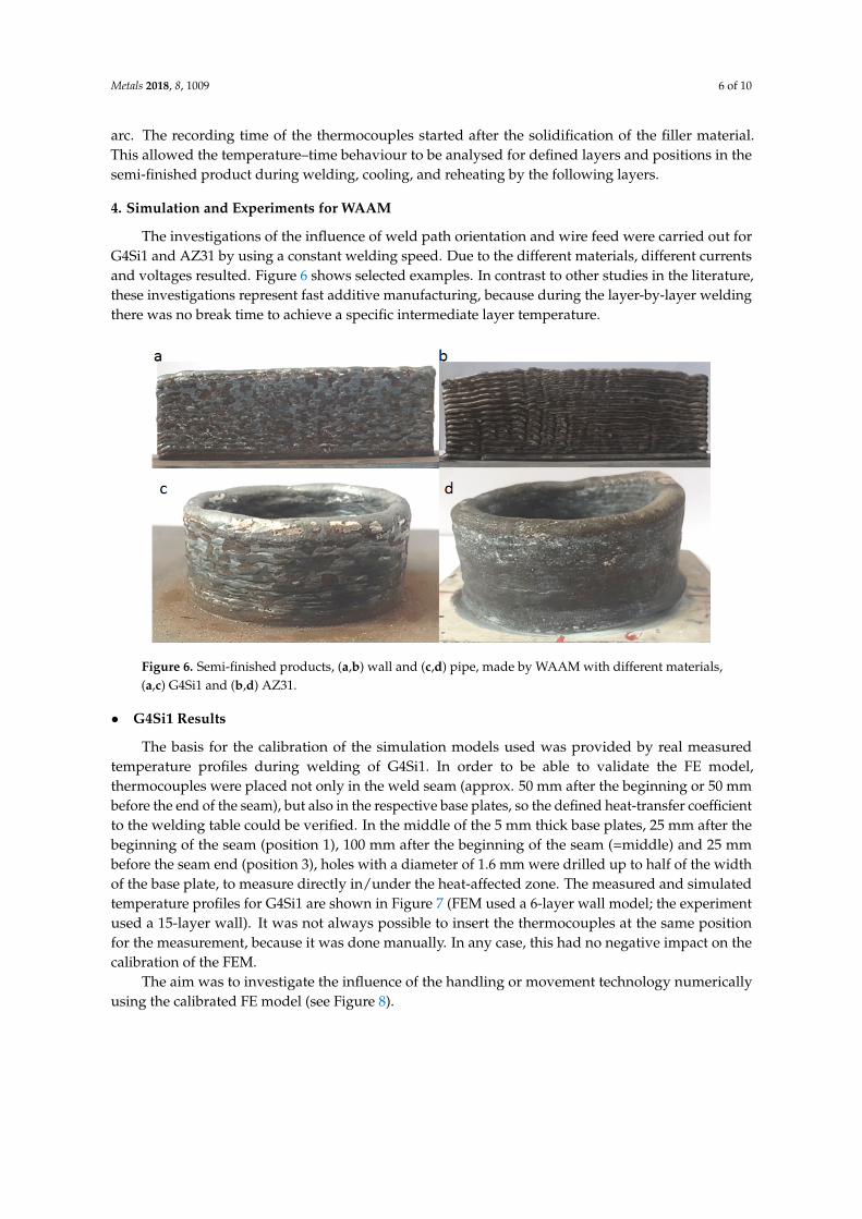
The investigations of the influence of weld path orientation and wire feed were carried out forG4Si1 and AZ31 by using a constant welding speed. Due to the different materials, different currentsand voltages resulted. Figure 6 shows selected examples. In contrast to other studies in the literature,these investigations represent fast additive manufacturing, because during the layer-by-layer weldingthere was no break time to achieve a specific intermediate layer temperature.
Materials 2018, 11, x FOR PEER REVIEW 6 of 10
The investigations of the influence of weld path orientation and wire feed were carried out for G4Si1 and AZ31 by using a constant welding speed. Due to the different materials, different currents and voltages resulted. Figure 6 shows selected examples. In contrast to other studies in the literature, these investigations represent fast additive manufacturing, because during the layer-by-layer welding there was no break time to achieve a specific intermediate layer temperature.
Figure 6. Semi-finished products, (a,b) wall and (c,d) pipe, made by WAAM with different materials, (a,c) G4Si1 and (b,d) AZ31.
• G4Si1 Results
The basis for the calibration of the simulation models used was provided by real measured temperature profiles during welding of G4Si1. In order to be able to validate the FE model, thermocouples were placed not only in the weld seam (approx. 50 mm after the beginning or 50 mm before the end of the seam), but also in the respective base plates, so the defined heat-transfer coefficient to the welding table could be verified. In the middle of the 5 mm thick base plates, 25 mm after the beginning of the seam (position 1), 100 mm after the beginning of the seam (=middle) and 25 mm before the seam end (position 3), holes with a diameter of 1.6 mm were drilled up to half of the width of the base plate, to measure directly in/under the heat-affected zone. The measured and simulated temperature profiles for G4Si1 are shown in Figure 7 (FEM used a 6-layer wall model; the experiment used a 15-layer wall). It was not always possible to insert the thermocouples at the same position for the measurement, because it was done manually. In any case, this had no negative impact on the calibration of the FEM.
Figure 7. Comparison of measured (solid line) and simulated (dotted line) temperatures of the discontinuous welding process for G4Si1 with vwire = 5.0 m/min and vwelding = 40 cm/min.
Figure 6. Semi-finished products, (a,b) wall and (c,d) pipe, made by WAAM with different materials,(a,c) G4Si1 and (b,d) AZ31.
• G4Si1 Results
The basis for the calibration of the simulation models used was provided by real measuredtemperature profiles during welding of G4Si1. In order to be able to validate the FE model,thermocouples were placed not only in the weld seam (approx. 50 mm after the beginning or 50 mmbefore the end of the seam), but also in the respective base plates, so the defined heat-transfer coefficientto the welding table could be verified. In the middle of the 5 mm thick base plates, 25 mm after thebeginning of the seam (position 1), 100 mm after the beginning of the seam (=middle) and 25 mmbefore the seam end (position 3), holes with a diameter of 1.6 mm were drilled up to half of the widthof the base plate, to measure directly in/under the heat-affected zone. The measured and simulatedtemperature profiles for G4Si1 are shown in Figure 7 (FEM used a 6-layer wall model; the experimentused a 15-layer wall). It was not always possible to insert the thermocouples at the same positionfor the measurement, because it was done manually. In any case, this had no negative impact on thecalibration of the FEM.
The aim was to investigate the influence of the handling or movement technology numericallyusing the calibrated FE model (see Figure 8).

Metals 2018, 8, 1009 7 of 10
Materials 2018, 11, x FOR PEER REVIEW 6 of 10
The investigations of the influence of weld path orientation and wire feed were carried out for G4Si1 and AZ31 by using a constant welding speed. Due to the different materials, different currents and voltages resulted. Figure 6 shows selected examples. In contrast to other studies in the literature, these investigations represent fast additive manufacturing, because during the layer-by-layer welding there was no break time to achieve a specific intermediate layer temperature.
Figure 6. Semi-finished products, (a,b) wall and (c,d) pipe, made by WAAM with different materials, (a,c) G4Si1 and (b,d) AZ31.
• G4Si1 Results
The basis for the calibration of the simulation models used was provided by real measured temperature profiles during welding of G4Si1. In order to be able to validate the FE model, thermocouples were placed not only in the weld seam (approx. 50 mm after the beginning or 50 mm before the end of the seam), but also in the respective base plates, so the defined heat-transfer coefficient to the welding table could be verified. In the middle of the 5 mm thick base plates, 25 mm after the beginning of the seam (position 1), 100 mm after the beginning of the seam (=middle) and 25 mm before the seam end (position 3), holes with a diameter of 1.6 mm were drilled up to half of the width of the base plate, to measure directly in/under the heat-affected zone. The measured and simulated temperature profiles for G4Si1 are shown in Figure 7 (FEM used a 6-layer wall model; the experiment used a 15-layer wall). It was not always possible to insert the thermocouples at the same position for the measurement, because it was done manually. In any case, this had no negative impact on the calibration of the FEM.
Figure 7. Comparison of measured (solid line) and simulated (dotted line) temperatures of the discontinuous welding process for G4Si1 with vwire = 5.0 m/min and vwelding = 40 cm/min.
Figure 7. Comparison of measured (solid line) and simulated (dotted line) temperatures of thediscontinuous welding process for G4Si1 with vwire = 5.0 m/min and vwelding = 40 cm/min.
Materials 2018, 11, x FOR PEER REVIEW 7 of 10
The aim was to investigate the influence of the handling or movement technology numerically using the calibrated FE model (see Figure 8).
Figure 8. Comparison of measured and simulated temperatures depending on welding orientation for G4Si1 with vwire = 5.0 m/min and vwelding = 40 cm/min: (a) discontinuous/unidirectional; (b) continuous/multidirectional.
The continuous process was significantly faster, because there was no need to move back to the subsequent starting position after finishing the welding of each layer. The comparison between simulation and experiment shows—particularly in the tests with steel filler material—that the maximum temperature cannot really be identified, because the thermocouples were not designed for the melting point of the steel, and the inertia of the measuring sensors meant they did not even record the short-term maximum temperature. However, the thermocouples were very important for the description of the cooling and reheating behaviour of each layer. Thereby, the thermal behaviour could be detected and compared with the simulated results. The analysis of the temperatures in the base plate shows that the thermal cycle oscillates more at the lower layer level. During the processes, the heating and cooling lay on a near steady state level, because the heat-affected zone was moved to higher layers and an increasing heat flow took place via the outside of the wall.
The quality of the FE results compared to the real tests was good in all cases. One result is that the welding orientation has an influence on the temperature profile and the wall geometry. During continuous multi-layered welding, the beginning and the end—depending on position—are exposed to the heat input twice within a short time and this input is symmetrical in both sides. In contrast, the welding speed and local heat input in discontinuous welding is the same in each layer, but the weld is not symmetrical. The base layer is colder at the beginning of the weld. As a result, the wetting behaviour is decreased and the viscosity is higher. The local build-up rate in the z-direction is therefore high. During welding, the base layer gets hotter. Simultaneously, the heat accumulation at the end is the highest. Since the welding power is constant, the weld acts on a continuously increasing base-material temperature level. The wetting behaviour therefore increases and the viscosity decreases. The local build-up rate in the upwards direction is therefore lower. The real samples therefore look different depending on the welding path direction, especially at the beginning, or rather, the end (see Figure 9).
Figure 8. Comparison of measured and simulated temperatures depending on welding orientationfor G4Si1 with vwire = 5.0 m/min and vwelding = 40 cm/min: (a) discontinuous/unidirectional;(b) continuous/multidirectional.
The continuous process was significantly faster, because there was no need to move back to thesubsequent starting position after finishing the welding of each layer. The comparison betweensimulation and experiment shows—particularly in the tests with steel filler material—that themaximum temperature cannot really be identified, because the thermocouples were not designedfor the melting point of the steel, and the inertia of the measuring sensors meant they did not evenrecord the short-term maximum temperature. However, the thermocouples were very important forthe description of the cooling and reheating behaviour of each layer. Thereby, the thermal behaviourcould be detected and compared with the simulated results. The analysis of the temperatures in thebase plate shows that the thermal cycle oscillates more at the lower layer level. During the processes,the heating and cooling lay on a near steady state level, because the heat-affected zone was moved tohigher layers and an increasing heat flow took place via the outside of the wall.
The quality of the FE results compared to the real tests was good in all cases. One result is thatthe welding orientation has an influence on the temperature profile and the wall geometry. Duringcontinuous multi-layered welding, the beginning and the end—depending on position—are exposedto the heat input twice within a short time and this input is symmetrical in both sides. In contrast,the welding speed and local heat input in discontinuous welding is the same in each layer, but theweld is not symmetrical. The base layer is colder at the beginning of the weld. As a result, the wettingbehaviour is decreased and the viscosity is higher. The local build-up rate in the z-direction is thereforehigh. During welding, the base layer gets hotter. Simultaneously, the heat accumulation at the endis the highest. Since the welding power is constant, the weld acts on a continuously increasing
Metals 2018, 8, 1009 8 of 10
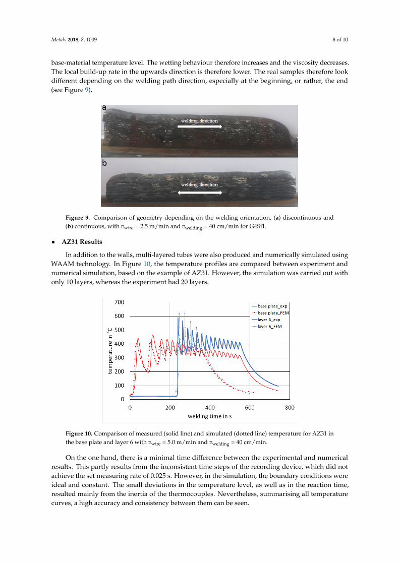
base-material temperature level. The wetting behaviour therefore increases and the viscosity decreases.The local build-up rate in the upwards direction is therefore lower. The real samples therefore lookdifferent depending on the welding path direction, especially at the beginning, or rather, the end(see Figure 9).Materials 2018, 11, x FOR PEER REVIEW 8 of 10
Figure 9. Comparison of geometry depending on the welding orientation, (a) discontinuous and (b) continuous, with vwire = 2.5 m/min and vwelding = 40 cm/min for G4Si1.
• AZ31 Results
In addition to the walls, multi-layered tubes were also produced and numerically simulated using WAAM technology. In Figure 10, the temperature profiles are compared between experiment and numerical simulation, based on the example of AZ31. However, the simulation was carried out with only 10 layers, whereas the experiment had 20 layers.
Figure 10. Comparison of measured (solid line) and simulated (dotted line) temperature for AZ31 in the base plate and layer 6 with vwire = 5.0 m/min and vwelding = 40 cm/min.
On the one hand, there is a minimal time difference between the experimental and numerical results. This partly results from the inconsistent time steps of the recording device, which did not achieve the set measuring rate of 0.025 s. However, in the simulation, the boundary conditions were ideal and constant. The small deviations in the temperature level, as well as in the reaction time, resulted mainly from the inertia of the thermocouples. Nevertheless, summarising all temperature curves, a high accuracy and consistency between them can be seen.
5. Conclusions
The experimental and numerical investigations on walls and tubes of G4Si1 and AZ31, using CMT for WAAM, have shown that the welding orientation has a critical influence on the temperature field as well as on the component geometry. The aim was the experimental, but especially the numerical, investigations of welding parameters and their influence on temperature development. For realistic numerical simulation, all temperature-dependent material data were first determined without database material but with samples, which have comparable microstructure to the WAAM
Figure 9. Comparison of geometry depending on the welding orientation, (a) discontinuous and(b) continuous, with vwire = 2.5 m/min and vwelding = 40 cm/min for G4Si1.
• AZ31 Results
In addition to the walls, multi-layered tubes were also produced and numerically simulated usingWAAM technology. In Figure 10, the temperature profiles are compared between experiment andnumerical simulation, based on the example of AZ31. However, the simulation was carried out withonly 10 layers, whereas the experiment had 20 layers.
Materials 2018, 11, x FOR PEER REVIEW 8 of 10
Figure 9. Comparison of geometry depending on the welding orientation, (a) discontinuous and (b) continuous, with vwire = 2.5 m/min and vwelding = 40 cm/min for G4Si1.
• AZ31 Results
In addition to the walls, multi-layered tubes were also produced and numerically simulated using WAAM technology. In Figure 10, the temperature profiles are compared between experiment and numerical simulation, based on the example of AZ31. However, the simulation was carried out with only 10 layers, whereas the experiment had 20 layers.
Figure 10. Comparison of measured (solid line) and simulated (dotted line) temperature for AZ31 in the base plate and layer 6 with vwire = 5.0 m/min and vwelding = 40 cm/min.
On the one hand, there is a minimal time difference between the experimental and numerical results. This partly results from the inconsistent time steps of the recording device, which did not achieve the set measuring rate of 0.025 s. However, in the simulation, the boundary conditions were ideal and constant. The small deviations in the temperature level, as well as in the reaction time, resulted mainly from the inertia of the thermocouples. Nevertheless, summarising all temperature curves, a high accuracy and consistency between them can be seen.
5. Conclusions
The experimental and numerical investigations on walls and tubes of G4Si1 and AZ31, using CMT for WAAM, have shown that the welding orientation has a critical influence on the temperature field as well as on the component geometry. The aim was the experimental, but especially the numerical, investigations of welding parameters and their influence on temperature development. For realistic numerical simulation, all temperature-dependent material data were first determined without database material but with samples, which have comparable microstructure to the WAAM
Figure 10. Comparison of measured (solid line) and simulated (dotted line) temperature for AZ31 inthe base plate and layer 6 with vwire = 5.0 m/min and vwelding = 40 cm/min.
On the one hand, there is a minimal time difference between the experimental and numericalresults. This partly results from the inconsistent time steps of the recording device, which did notachieve the set measuring rate of 0.025 s. However, in the simulation, the boundary conditions wereideal and constant. The small deviations in the temperature level, as well as in the reaction time,resulted mainly from the inertia of the thermocouples. Nevertheless, summarising all temperaturecurves, a high accuracy and consistency between them can be seen.

Metals 2018, 8, 1009 9 of 10
5. Conclusions
The experimental and numerical investigations on walls and tubes of G4Si1 and AZ31, using CMTfor WAAM, have shown that the welding orientation has a critical influence on the temperature fieldas well as on the component geometry. The aim was the experimental, but especially the numerical,investigations of welding parameters and their influence on temperature development. For realisticnumerical simulation, all temperature-dependent material data were first determined without databasematerial but with samples, which have comparable microstructure to the WAAM process. On the basisof these thermal material behaviours followed modelling, and then final implementation in the MSCMarc software. Based on this, it was possible to simulate the temperature profile in the semi-finishedproducts very well, when the seam geometry and heat source according to Goldak were defined.Purely for convenience, the welding table was not modelled, but its heat-transfer coefficient was takeninto account. The simulated temperatures in the components can be the basis for the prediction ofdistortion, residual stresses and, if necessary, coupling to microstructural phenomena (e.g., multiplephase transformation according to t8-5-time for steel grades). These effects are being analysed anddescribed in ongoing research work.
Author Contributions: M.G., A.H. and K.H. designed and realized the experiments; A.H. and K.H. identifiedand modeled the material properties; M.G. made the numerical simulation of WAAM processes; M.G. wrote thepaper; B.A. and P.M. are the project coordinators and supervisors.
Funding: This research was funded by German Academic Exchange Service (DAAD) grant number 57347629.
Acknowledgments: These results are part of the subproject “Digital Engineering in Different Cultures” from theGerman Academic Exchange Service (DAAD) project “Higher Education Dialogue with People from IslamicCountries”. The authors thank DAAD for the financial support. The authors thank also the colleagues from theInstitute of Metal Forming and Professorship of Technical Thermodynamics of TU Bergakademie Freiberg fortheir support with material characterization.
Conflicts of Interest: The authors declare no conflict of interest.
References
1. Gebhardt, A. Additive Fertigungsverfahren: Additive Manufacturing und 3D-Drucken für Prototyping-Tooling-Produktion; Carl Hanser Verlag: Munich, Germany, 2016; ISBN 978-3-446-44401-0.
2. EN ISO 17926-2:2015. Additive Manufacturing. General principles. Part 2: Overview of Process Categories andFeedstock; International Organization for Standardization: Geneva, Switzerland, 2015.
3. Ogino, Y.; Asia, S.; Hirata, Y. Numerical simulation of WAAM process by a GMAW weld pool model.Weld. World 2018, 62, 393–401. [CrossRef]
4. Frazier, W. Metal additive manufacturing: A review. J. Mater. Eng. Perform. 2014, 23, 1917–1928. [CrossRef]5. Ding, J.; Pan, Z.; Cuiuri, D.; Li, H. Thermo-mechanical analysis of wire and arc additive layer manufacturing
process on large multi-layer parts. Comput. Mater. Sci. 2011, 50, 3315–3322. [CrossRef]6. Brandl, E.; Baufeld, B.; Leyens, C.; Gault, R. Additive manufactured Ti-6Al-4V using welding
wire—Comparison of laser and arc beam deposition and evaluation with respect to aerospace materialspecifications. Physic. Procedia 2010, 5, 595–606. [CrossRef]
7. Derekar, K.S. A review of wire arc additive manufacturing and advances in wire arc additive manufacturingof aluminium. Mater. Sci. Technol. 2018, 34, 895–916. [CrossRef]
8. Kazanas, P.; Deherkar, P.; Almeida, P.; Lockett, H.; Williams, S. Fabrication of geometrical features using wireand arc additive manufacture. Proc. Inst. Mech. Eng. Part B J. Eng. Manuf. 2012, 226, 1042–1051. [CrossRef]
9. Schmidt, M.; Merklein, M.; Bourell, D.; Dimitrov, D.; Hausotte, T.; Wegener, K.; Overmeyer, L.; Vollertsen, F.;Levy, G.-N. Laser based additive manufacturing in industry and academia. CIRP Ann. Manuf. Technol. 2017,66, 561–583. [CrossRef]
10. Szost, B.A.; Terzi, S.; Martina, F.; Boisselier, D.; Prytuliak, A.; Pirling, T.; Hofmann, M.; Jarvis, D.J.A comparative study of additive manufacturing techniques: Residual stress and microstructural analysis ofCLAD and WAAM printed Ti-6Al-4V components. Mater. Des. 2016, 89, 559–567. [CrossRef]

Metals 2018, 8, 1009 10 of 10
11. Bock, F.E.; Froend, M.; Herrnring, J.; Enz, J.; Kashaev, N.; Klusemann, B. Thermal analysis of laser additivemanufacturing of aluminium alloys: Experiment and simulation. AIP Conf. Proc. 2018, 1960, 140004.[CrossRef]
12. Tran, H.-S.; Tchuindjang, J.T.; Paydas, H.; Mertens, A.; Jardin, R.T.; Duchêne, L.; Carrus, R.;Lecomte-Beckers, J.; Habraken, A.M. 3D thermal finite element analysis of laser cladding processed Ti-6Al-4Vpart with microstructural correlations. Mater. Des. 2017, 128, 130–142. [CrossRef]
13. Ferro, P.; Berto, F.; James, N.M. Asymptotic residual stress distribution induced by multipass weldingprocesses. Int. J. Fatigue 2017, 101, 421–429. [CrossRef]
14. Graf, M.; Pradjadhiana, K.P.; Haelsig, A.; Manurung, Y.H.P.; Awiszus, B. Numerical simulation of metallicwire arc additive manufacturing (WAAM). AIP Conf. Proc. 2018, 1960, 140010. [CrossRef]
15. Schwenk, C. FE-Simulation des Schweißverzugs Laserstrahlgeschweißter Dünner Bleche, Dissertation; FraunhoferIWM: Freiburg im Breisgau, Germany, 2001.
16. Denlinger, E.R. Thermo-Mechanical Model Development and Experimental Validation for Metallic Parts inAdditive Manufacturing. Ph.D. Thesis, The Pennsylvania State University, State College, PA, USA, 2015.
17. Miehe, A. Numerical Investigation of Horizontal Twin-Roll Casting of the Magnesium Alloy AZ31.Ph.D. Thesis, Technische Universität Bergakademie, Freiberg, Germany, 2014.
18. Dieckmann, U. Calculation of steeldata using JMatPro. COMAT Recent Trends Struct. Mater. 2012, 21, 11.19. Montevecchi, F.; Venturini, G.; Scippa, A.; Campatelli, G. Finite element modelling of wired-arc additive
manufacturing process. Procedia CIRP 2016, 55, 109–114. [CrossRef]20. Hoefer, K.; Haelsig, A.; Mayr, P. Arc-based additive manufacturing of steel components—Comparison of
wire- and powder-based variants. Weld. World 2017, 62, 243–247. [CrossRef]21. Meyer, T. Ein Beitrag zur Auslegung temperierter Tiefziehwerkzeuge für die Umformung von
Magnesiumfeinblechen. Ph.D. Thesis, Technische Universität Bergakademie, Freiberg, Germany, 1975.22. Goldak, J.; Chakravarti, A.; Bibby, M. A new finite element model for welding heat source. Metall. Trans. B
1984, 15, 299–305. [CrossRef]
© 2018 by the authors. Licensee MDPI, Basel, Switzerland. This article is an open accessarticle distributed under the terms and conditions of the Creative Commons Attribution(CC BY) license (http://creativecommons.org/licenses/by/4.0/).