thermally safe operation of liquid–liquid semibatch reactors. part i: single kinetically...

Chemical Engineering Science 60 (2005) 3309–3322

www.elsevier.com/locate/ces

Thermally safe operation of liquid–liquid semibatch reactors. Part I:Single kinetically controlled reactions with arbitrary reaction order

Francesco Maestri, Renato Rota∗

Politecnico di Milano, Dip. di Chimica, Materiali e Ingegneria Chimica “G. Natta”, via Mancinelli 7, 20131 Milano, Italy

Received 20 September 2004; received in revised form 26 November 2004; accepted 3 December 2004Available online 19 March 2005

Abstract

The thermally safe operation of an indirectly cooled semibatch reactor in which an exothermic reaction occurs corresponds to conditionsof potentially very high effective reaction rate compared to the dosing rate of the coreactant, whose accumulation in the reaction systemis consequently small. On this basis it is possible to build boundary diagrams in terms of suitable dimensionless parameters, whichsummarize all the possible thermal behaviors of the reactor and can be used for safe scaleup purposes.

In this work the influence of reaction kinetics on the shape and location of boundary diagrams for a single liquid–liquid reaction inthe slow regime is discussed. First of all, the theory of boundary diagrams, originally developed for (1,1) reaction order, is extended to ageneric(n,m) rate of reaction expression. Then it is shown that in many practical systems, using boundary diagrams based on (1,1) reactionorder can lead to both unsafe and unnecessary (from a safety point of view) low-production operating conditions. New boundary diagramsfor a few (n,m) reaction orders are presented. Some rules-of-thumb are also discussed to identify in which cases a boundary diagramdeveloped for a given(n,m) reaction order can be reasonably used to approximate the real kinetic behavior of the system of interest.

Moreover, since building a boundary diagram for the specific kinetics considered can be necessary, a simple and general procedure forbuilding such diagrams that can be easily implemented in a computer code is also presented.� 2005 Elsevier Ltd. All rights reserved.

Keywords:Semibatch reactors; Boundary diagrams; Kinetics; Runaway; Safety; Scaleup

1. Introduction

Runaway in chemical batch and semibatch reactors in-volving exothermic reactions is very frequent; for instance,in a typical EU country more than 100 runaways are expectedto occur annually (Benuzzi and Zaldivar, 1991). Fortunately,few accidents leads to serious consequences to either theworkers or the inhabitants of the neighborhood. However,when strong runaways occur, the consequences can be reallyserious, as happened, for instance, in 1976 in Seveso, Italy.

This motivates the huge amount of work that has beendone on runaway phenomena in chemical batch and semi-batch reactors, for developing simple and reliable procedures

∗ Corresponding author. Tel.: +39 0223993154; fax: +39 0223993180.E-mail address:[email protected](R. Rota).

0009-2509/$ - see front matter� 2005 Elsevier Ltd. All rights reserved.doi:10.1016/j.ces.2004.12.046

to scale up chemical processes from laboratory to industrialscale.

The main problem to face in practice is that in fine chem-ical industries, which produce very different amounts of awide range of chemical compounds, it is usually not possi-ble, because of time and money constraints, to investigatein detail the kinetics of all the reactions involved. This callsfor a procedure that must be not only reliable but also sim-ple, and explains why, in spite of the progress that has beenmade in understanding runaway phenomena, the problemhas not been solved yet for practice, so that runaways stilloccur (Westerterp and Molga, 2004).

It should be mentioned that the incorrect scale up of theprocess is not the only responsible for runaways. Otherevents can initiate a runaway, such as those related to humanfactors, maintenance, failure of the control system, agita-tor breakdown, etc. However, these events can be easily

http://www.elsevier.com/locate/ces

mailto:[email protected]

3310 F. Maestri, R. Rota / Chemical Engineering Science 60 (2005) 3309–3322

identified through standard techniques used for hazard iden-tification processes, such as the hazard and operability (HA-ZOP) analysis. Moreover, they can be handled enforcing asuitable design, working and maintenance procedure. Con-sequently, a correct scaleup is the key point for runawayprevention.

When the heat effects associated with a chemical reactionare high, the process cannot be carried out safely in a batchreactor (Steinbach, 1999). The rate of heat evolution can becontrolled by adding one of the reactants slowly to the othercomponent already present in the reactor, that is, by usingan indirectly cooled semibatch reactor (SBR). The dosingrate of one of the reactants (usually called coreactant) mustbe slow enough so that the cooling system can remove allthe heat released.

The first studies about the thermally safe operation ofSBRs were conducted byHugo and Steinbach (1985, 1986).Their work, based onhomogeneousreaction systems, in-troduced the accumulation criterion for the analysis of thethermal behavior of SBRs: accumulation of the coreactantin the system arises from a not negligible characteristic timeof the chemical reaction, compared with that of the coreac-tant supply and must be kept at sufficiently low values toavoid the thermal loss of control of the reactor (runaway).

If the coreactant accumulates in the reactor, the systemswitches from semibatch to batch-like conditions and thecooling system cannot control the heat evolution anymore.

Steensma and Westerterp (1988, 1990, 1991)extended theresults obtained by Hugo and Steinbach toheterogeneous(liquid–liquid) SBRs, introducing the concept of target tem-perature and producing the so-called boundary diagrams forsingle reactions (both in the slow or fast regime) of (1,1)reaction order kinetics, that is of the typer = kCACB.

Boundary diagrams define, in a suitable dimensionlessspace, the regions where different reactor behaviors are ex-pected. In particular, runaway and inherently safe regionsare defined, allowing for identifying safe and dangerous op-erating conditions.

van Woezik and Westerterp (2000, 2001)extended theconcepts introduced by Steensma and Westerterp to the caseof multiple (consecutive) reactions, studying both theoret-ically and experimentally the nitric acid oxidation of 2-octanol to 2-octanone with further oxidation of the desiredreaction product to carboxylic acids.

Recently, the work of Steensma and Westerterp on slowliquid–liquid reaction systems was improved byWesterterpand Molga (2004), with particular emphasis on how to usein practice the boundary diagrams and on how to defineinherently safe operating conditions.

As previously mentioned, detailed information on the re-action mechanism and kinetics are seldom available in prac-tice. However, modeling the behavior of a liquid–liquid SBRrequires the knowledge of the reaction kinetics, at least interms of a lumped overall reaction. Such information canbe obtained through calorimetric (e.g., RC1) experimentscarried out in the slow reaction (microkinetic) regime. This

means that some laboratory experimental work cannot beavoided (Westerterp and Molga, 2004). The main aim of de-veloping simple scaleup procedures is to keep such an ex-perimental effort as low as possible. Boundary diagrams area suitable tool to achieve this goal.

Experimental data are usually interpreted through power-law rate of reaction expressions with(n,m) reaction orders:r = kCn

ACmB . In spite of the fact that(n,m) usually differ

from (1,1), boundary diagrams have been developed till nowonly for the (1,1) case, and some rules-of-thumb have beenproposed to use the (1,1) boundary diagrams for a generic(n,m) reaction order (Westerterp and Molga, 2004). Con-sequently, the main aim of this work is to analyze in detailthe influence of the reaction orders on the boundary dia-grams, providing runaway and inherently safe regions forsome(n,m) couples. These boundary diagrams can be usedas a guide for a preliminary analysis of any reaction or-der. Moreover, to allow for a more rigorous analysis of ageneric(n,m) reaction order, a practical procedure for build-ing boundary diagrams for generic(n,m) reaction ordersis also presented, with particular attention to the physicalmeaning of the various dimensionless parameters required.

2. Mathematical model

Developing a boundary diagram for a generic(n,m) re-action order and discussing the physical meaning of the di-mensionless parameters introduced to define the space whererunaway or inherently safe regions are defined requires apreliminary discussion on how the investigated process canbe modeled.

We assume that at time equal to zero the feed of the core-actant A to an SBR filled with a given amount of componentB is started at a constant rate, until the stoichiometric ratiobetween the two species is reached, according to the overallstoichiometry:

�AA + �BB → C + �DD. (1)

The process involves two liquid phases: a continuousphase and a dispersed phase (in the following referred to,respectively, as the “c” phase and the “d” phase).

We further assume that the microkinetic rate expressionof reaction (1) can be described by a generic power-lawexpression:

r = kn,mCnAC

mB . (2)

A simple mathematical model can be formulated assumingthat:

(1) the reaction mass is perfectly macromixed;(2) the influence of the chemical reaction on the volume of

the single phase is negligible;(3) no phase inversions occur;(4) the solubility of the species A and C in the continuous

phase, c, and of components B and D in the dispersed

F. Maestri, R. Rota / Chemical Engineering Science 60 (2005) 3309–3322 3311

phase, d, is small (in other words, species A and C arealmost all in phase d, whereas species B and D arepresent almost only in phase c);

(5) the chemical reaction takes place only in one of the twoliquid phases: this situation is very common in manyindustrial processes (such as nitrations and oxidations),in which the catalyst (typically a strong acid) is presentonly in one phase;

(6) the heat effects are associated with the chemical reactiononly;

(7) at the beginning, the reaction mass is at the mean coolanttemperature,Tcool, which is assumed to remain constantfor the whole duration of the process (that is, the reactoroperates in isoperibolic conditions).

The mass balance equation for theith chemical species is

dnidt

= Fi,D + �i reffVr . (3)

The molar feed rate,Fi,D, differs from zero only for thespecies A during the supply period and, as usual, the stoi-chiometric coefficient,�i , is negative for reactants and pos-itive for products. Moreover, the number of moles in the re-actor att =0, ni,0, is different from zero only for species B.The effective reaction rate,reff , depends on the microkineticrate expression, the phase in which the reaction takes placeand the controlling step among the chemical reaction, theinterphase mass transfer and the supply of the coreactant.

In this work, we investigate the slow reaction regime,which means that the interphase mass transfer phenomenanever control the effective rate of the process, resulting innearly uniform concentration profiles in both the phases.

Since we assume to feed a stoichiometric amount of core-actant, the quantity of species A supplied to the reactorthroughout the dosing period,tD, (or, equivalently, from thebeginning to the dimensionless timeϑ = t/tD = 1) can becomputed asnA,1 = FA,DtD = (�A/�B)nB,0.

Moreover, since we are considering a single reaction, onescalar, such as the conversion of species B,�B=1−nB/nB,0,suffices to define the extent of the reaction.

Performing suitable combinations of the mass balanceequations (3) and integrating the resulting differentialequations, it is possible—using assumptions (2) and (4)

Table 1Expressions of the reactivity enhancement factor, RE, and of the function,f , for slow reactions taking place in the dispersed or continuous phase,(requirements for slow regime are also reportedWesterterp et al., 1984)

Slow reaction in the dispersed phase, d Slow reaction in the continuous phase, c

REslow,c/d

(�B

�A

)1−n

mmB

(�B

�A

)1−n

mnA

fslow,c/d(ϑ − �B)

n(1 − �B)m

(�ϑ)n−1(ϑ − �B)

n(1 − �B)m

(�ϑ)n

Check for slow reaction regimeHad = 1

kL,B

√2

m+1 kn,mDL,BCm−1B,Id

CnA,d <0.3

CB,d/CB,Id >0.95

Hac = 1

kL,A

√2

n+1 kn,mDL,ACn−1A,Ic

CmB,c<0.3

CA,c/CA,Ic >0.95

stated before—to derive the following equations, relating theconcentrations of A in the dispersed phase,CA,d, and of Bin the continuous phase,CB,c, to ϑ and�B:

CA,d = nB,0(ϑ − �B)�A/�B

VDϑ, (4)

CB,c = nB,0(1 − �B)

Vc. (5)

Moreover, the mass balance equation for the reactant B canbe rewritten as

d�B

dϑ= �BtD

nB,0reffVr . (6)

Along the line discussed bySteensma and Westerterp (1988,1990, 1991), this equation can be rewritten in the followingform:

d�B

dϑ= �ADa REslow,c/dfslow,c/d�n,m, (7)

whereDa = kn,m,RtDCn+m−1B,0 is the Damköhler number

for (n,m) order kinetics, which contains the physical in-formation about the dosing time, and�n,m = exp[�(1 −1/�)] is the dimensionless reaction rate constant, that isthe ratio of the reaction rate to the reaction rate evaluatedat a reference temperature,TR, with � = E/(RT R) and� = T/TR.

Introducing Eq. (2) in Eq. (7) and using relations (4)–(6),the expressions of the reactivity enhancement factor, RE,and of the function,f , can be easily derived for the casesof slow reaction taking place, respectively, in the dispersed(REslow,d and fslow,d) or in the continuous (REslow,c andfslow,c) phase.

These expressions, which are summarized inTable 1, alsoinvolve the relative volume increase throughout the dosingperiod, � = VD/Vc, as well as the distribution coefficient,mi , which is defined as the ratio between the equilibriumconcentrations of componenti in the two phases (moreprecisely, it is the ratio of the concentration of componenti in the phase in which its solubility is small to that in theother phase). The main difference with respect to the casen=m=1 is that now the functionfslow,c/d does not dependonly on� but also on the values ofn andm. This dependence


will reflect, as discussed in the following, on the shape andlocation of the boundary diagrams.

The energy balance equation for the reactor is

(ndCP,d + ncCP,c)dT

dt= FDCP,D(TD − T )

+ Vrreff(−�Hr )

− UA(T − Tcool), (8)

showing that the reactor temperature variations are the resultof three enthalpic contributions, associated with the dosingstream, the chemical reaction and the heat removal by thecoolant.

As done previously for the mass balance equation, usingEq. (7), the energy balance can be rewritten in the followingdimensionless form

(1 + RH �ϑ)d�dϑ

= ��ad,0d�B

dϑ− [U∗Da(1 + �ϑ) + �RH ]

× (� − �effcool), (9)

whereRH = �dCP,d/�cCP,c ≈ �DCP,D/�0CP,0 is the ratiobetween the volumetric thermal capacities of the dispersedand the continuous phase, respectively. Moreover, the reac-tion enthalpy has been expressed in the form of an adiabatictemperature rise,�Tad,0 = (−�Hr )nB,0/�B�cCP,cVc, and amodified Stanton number for the system has been defined asU∗Da = (UA)0tD/�cCP,cVc. Finally, an effective coolanttemperature has been introduced, which takes into accountthe enthalpic contributions of both the heat removal by thecoolant and the dosing stream,T eff

cool=U∗Da(1+�ϑ)Tcool+�RHTD/(U

∗Da(1 + �ϑ) + �RH).The numerical integration (carried out using the MAT-

LAB suite of programs) of Eqs. (7) and (9) with their ini-tial conditions generates the time evolutions of conversionand temperature in the reactor.Figs. 1and2 show, for thesake of example, the temperature–time profiles for differentreaction orders. We can see that the influence of the orderof reaction with respect to the dosed component,n, on thethermal behavior of the system is much greater than that ofthe order of reaction with respect to the reactant initiallycharged in the reactor,m. For the same set of parametersand the same initial conditions, a runaway situation can dis-appear for greater values ofn but not ofm. This is correct,since the reaction order with respect to the coreactant hasa direct influence on the accumulation of the coreactant it-self in the reactor: the higher the value ofn, the higher thereaction rates normally become for a given increase of theholdup of unreacted coreactant in the system. This fact obvi-ously counteracts the accumulation phenomenon and resultsin a safer operation of the reactor, as discussed in detail inthe following paragraphs.

3. Thermally safe operating conditions

The thermally safe operation of an SBR in which anexothermic reaction occurs corresponds to conditions in

Fig. 1. Temperature–time profiles in an SBR for a slow reaction in thedispersed phase.�A Da RE= 1.8, �= 0.4, �= 38, RH = 1, ��ad,0 = 0.6,Co=10. Coolant and dosing stream temperature values equal to the initialreactor temperature: (A) influence of the reaction order of the coreactant,n; and (B) influence of the reaction order of the reactant initially chargedin the reactor,m.

which the overall kinetics of the process is largely deter-mined by the dosing rate of the coreactant, whose accu-mulation in the system is consequently confined below acritical value.

This implies that the characteristic time of the chemicalreaction (eventually affected by the influence of interphasemass transfer) is much smaller than the characteristic timeof the coreactant supply. This can be quantified by intro-ducing the concept of target temperature,Tta (Steensma andWesterterp, 1988).

If we assume that the overall kinetics of the process iscompletely determined by the dosing rate of the coreactant,the mass balance (7) simplifies to

d�B

dϑ= 1. (10)


Fig. 2. Temperature–time profiles for a slow reaction in the continuousphase. Legend and other parameters as inFig. 1.

If we further assume that the reaction temperature evolutionis completely dominated by the heat removal contribution,we can introduce a quasi-steady-state assumption for thetemperature itself, which yields

d�dϑ

= 0. (11)

Looking at the right-hand side of the energy balance (9),this physically means that the characteristic time of the heatremoval from the system (related to both the cooling effi-ciency and the sensible heat of the dosing stream) is muchlower than that associated with the reaction enthalpy: theseoperating conditions minimize the time variations of the re-actor temperature, which consequently approaches zero asstated in Eq. (11).

Substituting these expressions into the energy balanceequation (9), we obtain the following temperature–time

relation, corresponding to the assumptions stated above:

� − �effcool =

��ad,0

U∗Da(1 + �ϑ) + �RH

. (12)

Even if it is natural to associate a “safe” operation of thereactor to the absence of temperature jumps above a “targettemperature”, it is basically arbitrary to give a quantitativedefinition of what an acceptable accumulation of the dosedcoreactant in the system is. Eq. (12) refers to a theoreti-cally negligible ratio between the characteristic times of thechemical reaction and the coreactant supply.

To take into account the unavoidable accumulation ofthe coreactant which occurs in every real system,Steensmaand Westerterp (1988)suggest—on the basis of the anal-ysis of a number of industrial cases—a 5% overestima-tion of this temperature difference and call the resultingtemperature–time relation target temperature,Tta:

�ta = �effcool + 1.05

��ad,0

U∗Da(1 + �ϑ) + �RH

. (13)

It should be mentioned that other criteria proposed in theliterature for identifying runaway conditions are intrinsicand consequently free from this limitation (cf.Varma et al.,1999).

Comparing now the real temperature evolution of an SBRwith the corresponding target temperature, it is possible toclassify the thermal behavior of the system from the safetypoint of view: the exceeding of the target temperature lineis regarded as a runaway and provides the starting pointfor building boundary diagrams on a suitable dimensionlessspace. The corresponding dimensionless groups can be iden-tified looking at the right-hand side of the energy balanceEq. (9). We can recognize an enthalpic contribution associ-ated with the chemical reaction:

Qr = ��ad,0d�B

dϑ(14)

and a combined enthalpic contribution which takes into ac-count the heat removal from the reactor by both the coolantand the dosing stream:

Qcool = [U∗Da(1 + �ϑ) + �RH ](� − �effcool). (15)

Following the same approach as in the classical explosiontheory ofSemenov (1940), we can quantify the entity of thetemperature dependence of the two contributions (14) and(15) by evaluating the corresponding temperature deriva-tives:

dQr

d�= ��ad,0�ADa REf�

��2 , (16)

dQcool

d�= U∗Da(1 + �ϑ) + �RH . (17)

The use of these derivatives can be simplified by introducingsome dimensionless quantities, that is a reactivity factor,


FR, which is mainly related to the reaction rate, an exother-micity factor,FE , which is mainly related to the adiabatictemperature rise, and a cooling factor,Fcool, related to thecooling potential:

FR = �ADa RE� = 1

f

d�B

dϑ, (18)

FE = ��ad,0��2 , (19)

Fcool = U∗Da(1 + �ϑ) + �RH , (20)

leading to a more compact expression of Eqs. (16) and (17):

dQr

d�= fFRFE , (21)

dQcool

d�= Fcool. (22)

It is easy to observe that, at the current value off , fordifferent sets of the parameters which appear in Eqs. (7) and(9), the same value of expression (21) can correspond to twoasymptotic situations and precisely:

(a) to a very high (theoretically infinite) value ofFR and avery low (theoretically approaching zero) value ofFE ;

(b) to a very low (theoretically approaching zero) value ofFR and a very high (theoretically infinite) value ofFE .

The situations (a) and (b), which generate the same instanta-neous value of dQr/d�, are on opposite sides from the safetypoint of view. Situation (a) corresponds to a very high reac-tion rate (which counteracts the accumulation of the core-actant in the system) and very low values of the activationenergy and/or the adiabatic temperature rise: regardless ofthe cooling potential this situation is always safe. Situation(b) implies the opposite and, regardless of the cooling po-tential, certainly results in a runaway.

Intermediate cases, characterized by finite values ofFR

andFE , cannot be classified (in terms of runaway or safeconditions) without relating them to the heat removal con-tribution from the system, dQcool/d�. The ratios of the re-activity and the exothermicity factor to the cooling factor,evaluated at the coolant temperature, are the two suitabledimensionless parameters to define the space where bound-ary diagrams can be reported. These ratios, called reactiv-ity, Ry , and exothermicity,Ex , numbers were introduced bySteensma and Westerterp (1988)and assume the followingexpressions:

Ry = FR

Fcool

∣∣∣∣ϑ=0

= �ADa RE�(�cool)

U∗Da + �RH

= �ADa RE�(�cool)

�(Co + RH), (23)

Ex = FE

Fcool

∣∣∣∣ϑ=0

= �

�2cool

��ad,0

U∗Da + �RH

= �

�2cool

��ad,0

�(Co + RH), (24)

where the cooling numberCo = U∗Da/� has also been in-troduced. The aforementioned asymptotic situations (a) and(b), reported in theRy vs. Ex space, imply that the left-upper region of the diagram always corresponds to safe con-ditions and that the right-bottom region always correspondsto runaway conditions.

The comparison between the temperature–time profile andthe corresponding target temperature line represents a use-ful way for classifying the thermal behavior of the system(Steensma and Westerterp, 1988). Given a set of values forthe parameters which appear in Eqs. (7) and (9), and solv-ing such equations for increasing values of the coolant tem-perature, it is possible to identify four typologies of thermalbehaviors of the reactor:

(1) for sufficiently low values of the coolant temperature,the maximum reaction temperature attained is lower thanthe local target value: this means that the reaction isnot ignited. In such a situation the accumulation of thecoreactant in the system reaches obviously high valuesbut the reaction is never fast enough to cause the loss ofcontrol of the system from the thermal point of view;

(2) as the coolant temperature increases, the maximum tem-perature “pinches” locally the target line: this situationis referred to as a marginal ignition;

(3) further increasing the coolant temperature, the reactionrate is at the same time not so high to keep the accumu-lation of the coreactant sufficiently low and not so lowto avoid—when the reaction itself ignites—the loss ofcontrol of the system from the thermal point of view.This situation implies maximum reaction temperatureslarger than the local target value and it is referred to asa runaway;

(4) as the coolant temperature still increases, the reactionrate becomes fast enough to keep the accumulation ofthe coreactant A in the system sufficiently low that norunaways can occur. The minimum coolant temperaturefor which the exceeding of the local target value by themaximum reaction temperature disappears is referred toas a quick onset, fair conversion, smooth temperatureprofile (QFS) situation (Steensma and Westerterp, 1988),because it is characterized by a temperature evolutionwhich quickly approaches the target line and remainsclose to it throughout the dosing period, at the end ofwhich the conversion�B is almost complete.

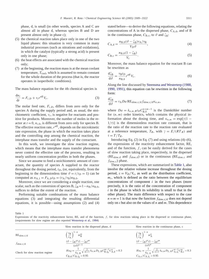
These regions can be reported on a boundary diagram asshown, for the sake of example, inFig. 3. The runawayregion is inside the continuous line and is surrounded bythe no ignition region (for lowRy values), the QFS region(for high Ry values) and by an inherently safe region. The


Fig. 3. Different SBR behavior regions and relation betweenRy andEx

with Tcool as a parameter.

letter is characterized by eitherEx values lower than theminimum Ex value of the runaway boundary,Ex,MIN , orby Ry values larger than the maximumRy value of therunaway boundary,Ry,QFS. The aforementioned asymptoticbehaviors (a) and (b) are also shown in the figure, the latteralways resulting in a runaway situation. This is the reasonwhy the runaway regions are not closed in the positiveEx

direction since a runaway always occurs forEx → ∞;the boundary diagrams reported in the figures extend untilrealistic values of the exothermicity number (Westerterp andMolga, 2004).

These diagrams can be easily used to solve two typologiesof problems:

1. for an existing reactor, operating at known values of thefixed parameters Co,RH , n andm, and in the slow re-action regime, the corresponding boundary diagram canbe used to identify thermally safe operating conditionswithout solving the mathematical model of the reactor;

2. the conclusions drawn for a given reactor from the useof the corresponding boundary diagram can be extendedto scaled up systems, provided that both the reactors arecharacterized by the sameCo, RH , n andm values andoperate in the same kinetic regime (in this case, the slowreaction regime).

As previously mentioned, to carry out a model simulationit is necessary to give a fixed value for all the dimen-sionless groups involved in the model, i.e. in Eqs. (7) and(9). Such dimensionless groups are�A Da RE, �, �, RH ,��ad,0, Co, n andm. As will be discussed in detail in Sec-tion 4, each boundary diagram involves a given range of theparameters:�A Da RE, �, � and��ad,0, but a fixed valueof the parametersCo, RH , n andm.

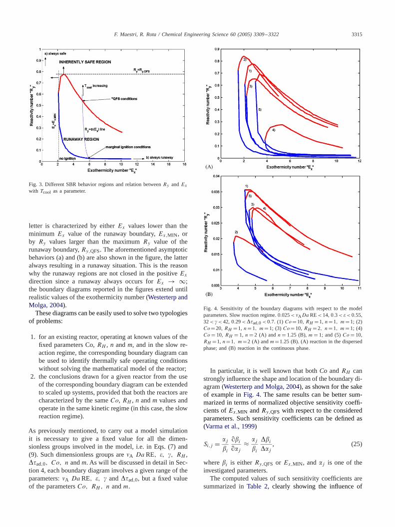
Fig. 4. Sensitivity of the boundary diagrams with respect to the modelparameters. Slow reaction regime. 0.025< �ADa RE<14, 0.3< �<0.55,32< �<42, 0.29<��ad,0 <0.7. (1)Co=10,RH =1, n=1, m=1; (2)Co=20,RH =1, n=1, m=1; (3) Co=10,RH =2, n=1, m=1; (4)Co = 10, RH = 1, n= 2 (A) andn= 1.25 (B), m= 1; and (5)Co = 10,RH =1, n=1, m=2 (A) andm=1.25 (B). (A) reaction in the dispersedphase; and (B) reaction in the continuous phase.

In particular, it is well known that bothCo andRH canstrongly influence the shape and location of the boundary di-agram (Westerterp and Molga, 2004), as shown for the sakeof example inFig. 4. The same results can be better sum-marized in terms of normalized objective sensitivity coeffi-cients ofEx,MIN andRy,QFS with respect to the consideredparameters. Such sensitivity coefficients can be defined as(Varma et al., 1999)

Si,j = �ji

�i

��j≈ �j

i

�i

��j, (25)

wherei is eitherRy,QFS or Ex,MIN , and�j is one of theinvestigated parameters.

The computed values of such sensitivity coefficients aresummarized inTable 2, clearly showing the influence of


Table 2Normalized sensitivity coefficients ofRy,QFS andEx,MIN computed from the data shown inFig. 4

Slow reaction in thedispersedphase, d Slow reaction in thecontinuousphase, c

Co RH n m Co RH n m

Ry,QFS 0.08 0.16 0.64 0.11 0.43 0.18 0.72 0.14Ex,MIN 0.28 0.07 0.82 0.44 0.17 0.03 0.27 0.08

the various parameters considered. From these data, we cansee that the influence of the reaction order on the values ofRy,QFSorEx,MIN can be larger than that of bothCoandRH .This conclusion is only partially tempered by noting thatthe range of variation ofCo in practical conditions is muchlarger than that of bothnandm(Westerterp and Molga, 2004;Steinbach, 1999): it is quite evident that the influence ofnandm on the shape and location of the boundary diagramscan be disregarded only as a first approximation.

However, the available boundary diagrams refer to reac-tion orders equal to (1,1) (Westerterp and Molga, 2004).This is obviously a limitation since reaction orders arenot always equal to one. The influence of the reactionorder values on the shape and location of the boundarydiagrams is shown inFigs. 5 and 6, referring to reac-tions in the dispersed and in the continuous phase, re-spectively. These diagrams are the results of a series ofsimulations extended to the following ranges of parame-ters: 0.025< �ADa RE<14, 0.3< �<0.55, 32< �<42,0.29<��ad,0 <0.7, Co = 10, RH = 1.

From these data we can observe that, when the order ofonly one component (that is, eithern or m) changes, the useof a boundary diagram obtained for a certain reaction orderis safe for reactions of larger order. Moreover, for both thecases (reaction taking place in the dispersed or in the contin-uous phase), variations in the order of the dosed coreactant,n, imply much larger differences in the extension of the cor-respondent runaway regions than variations of the reactionorder of the reactant initially charged in the reactor,m. Thisis obvious because the higher the reaction order of the dosedcoreactant, the faster the reaction rates become for a givenincrease (due to accumulation phenomena) of the holdup ofunreacted coreactant in the system: this counteracts directlythe accumulation of the coreactant itself in the reactor andconsequently can result in a narrower runaway region, evenfor relatively small increases ofn. Consequently, if betweenthe kinetic expression to which a boundary diagram refersto and that of the investigated system the order of the dosedcomponent changes, the conclusions drawn from the use ofthe diagram, even when safe, can be too conservative andhence unrealistic. For these reasons, the use of the correctboundary diagram is always advisable.

Finally it is quite evident that, for the same reaction or-der, the boundary diagram for the reaction taking place inthe dispersed phase shows always a runaway region largerthan the analogous diagram for the reaction occurring in thecontinuous phase. This is correct because for reactions tak-

Fig. 5. Boundary diagrams for slow(n,m) order reactions in thedispersed phase. 0.025< �ADa RE<14, 0.3< �<0.55, 32< �<42,0.29<��ad,0 <0.7, Co = 10, RH = 1: (A) influence of the reaction or-der of the coreactant,n; and (B) influence of the reaction order of thereactant initially charged in the reactor,m.

ing place in the dispersed phase, the reaction volume startsfrom zero and increases throughout the dosing period: thisimplies that the net production rates (i.e., thereffVr termin Eq. (6)) during the semibatch period are lower and theaccumulation of the coreactant is consequently higher.

It must be emphasized that the conclusions drawn aboveabout the safe use of an available boundary diagram for theanalysis of a system of different kinetics are true if between


Fig. 6. Boundary diagrams for slow(n,m) order reactions in the contin-uous phase. Legend and other parameters as inFig. 5.

the kinetic expression to which the boundary diagram refersto and that of the real system, only the reaction order of onecomponent (that is, eithern or m) changes, as is the case inFigs. 5and6.

If between the two kinetic expressions bothn and mchange, the overall reaction order (that is,n + m) is not asuitable parameter for establishing if the use of the boundarydiagram is safe: this comes from the different dependence ofthe shape and location of a boundary diagram onn andm,respectively, the former being much stronger. For the sakeof example, inFig. 7, the boundary diagram for a reactionoccurring in the dispersed phase withn=0.7 andm=1.4 iscompared with that forn=m=1. This figure clearly showsthat the runaway region for (0.7,1.4) is larger than that for(1,1) reaction order, even if the overall reaction order for theformer case is higher (that is, 0.7+ 0.4= 2.1 vs. 1+ 1= 2).

As previously discussed, while the influence of the re-action order of the reactant initially charged in the reactorcan be disregarded as a first approximation, the opposite

Fig. 7. Boundary diagrams for slow(n,m) order reactions in the dispersedphase. Legend and other parameters as inFig. 5.

is true for the reaction order of the coreactant. At a givenm value, increase inn leads to a significant narrowing ofthe runaway region, until, above a certainn, it is no morepossible to find a runaway region at the current values ofCo, RH , n, m in the investigated ranges of the parame-ters�A Da RE, �, �, ��ad,0. This is correct, since, as pre-viously shown, the higher then is, the more the reactionrates potentially increase as the holdup of unreacted A inthe system tends to grow. The aforementioned critical valueof n is lower for slow reactions occurring in the continuousphase: this is also correct since in this case the reaction vol-ume is maximum at the beginning of the supply period andthe reffVr term in Eq. (6) is consequently higher than forreactions occurring in the dispersed phase.

For practical use, boundary diagrams for different valuesof nare reported inFigs. 8–11. In these figures, the influenceof the cooling number and of the heat capacity ratio on thelocation and extension of a boundary diagram is shown forn = 0.5 and 2, for reactions taking place in the dispersedphase, and forn=0.5 and 1.25, for reactions taking place inthe continuous phase. Boundary diagrams for the basic caseof n = m = 1 have been already reported in the literature(Westerterp and Molga, 2004).

4. Procedure for building the boundary diagrams

As shown in the previous section, the use of a boundarydiagram built for a given reaction order can be unsafe forthe analysis of a system characterized by a different kinetics,and the comparison between the overall reaction orders isnot a suitable way for establishing that. Besides, even whenthe use of a boundary diagram for a different kinetics is safe,the conclusions drawn can be too conservative.

Consequently, the boundary diagrams reported in thiswork can be used as a first approximation, according to the


Fig. 8. Influence of the cooling number on the boundary diagramsshape and location. Slow reaction regime withn = 0.5, m = 1, RH = 1.0.025< �ADa RE<14, 0.3< �<0.55, 32< �<42, 0.29<��ad,0 <0.7:(A) reaction in the dispersed phase; and (B) reaction in the continuousphase.

rules-of-thumb given in the previous section and followingthe procedure discussed in detail elsewhere (Westerterp andMolga, 2004). On the other hand, there are several systemsfor which it could be useful to refer to the correct boundarydiagram. Once built, the boundary diagram for the real rateof reaction expression can be used for the a priori analysisof several changes in operating conditions of an existingreactor and for scaleup problems, provided that the remain-ing fixed parameters of the diagram (Co andRH ) and thekinetic regime (slow or fast reaction) are the same.

In the following, a simple and general procedure for build-ing the boundary diagrams for liquid–liquid SBR, in whicha single slow reaction of general power-law kinetics occurs,is presented. This procedure is not straightforward, since itinvolves the combination of many dimensionless parametersin several ways.

Fig. 9. Influence of the cooling number on the boundary diagrams shapeand location. Slow reaction regime withn = 2 (A) and n = 1.25 (B),m = 1, RH = 1. Legend and other parameters as inFig. 7.

As previously mentioned, eight dimensionless parametersappear in the mass and energy balance Eqs. (7) and (9) or,analogously, in expressions (23) and (24) of the reactivityand exothermicity numbers:�ADa RE, �, �, RH , ��ad,0,

Co, n andm. Assigning a value to each of these parame-ters in compliance with its accepted range and letting thecoolant temperature as a variable parameter, the functionaldependence between the exothermicity and reactivity num-bers,Ry = (Ex), is univocally identified. Eqs. (23) and(24) are the parametric form of this functional dependencesince they provide, for each value of the coolant tempera-ture, a couple of related values ofRy andEx , as shown, forthe sake of example, inFig. 3.

From Eqs. (23) and (24), it is evident that thesingleRy = (Ex) line (that is, a line representing the functionaldependence betweenRy andEx) on thesingleboundary di-agram (that is, forCo, RH , n, m values assigned and con-stant) is identified through the values of the following three


Fig. 10. Influence of the heat capacity ratio on the boundary diagramsshape and location. Slow reaction regime withn = 0.5, m = 1, Co = 10.0.025< �ADa RE<14, 0.3< �<0.55, 32< �<42, 0.29<��ad,0 <0.7:(A) reaction in the dispersed phase; and (B) reaction in the continuousphase.

dimensionless groups:

��ad,0

�(Co + RH)= const,

�ADa RE

�(Co + RH)= const,

� = const, (26)

that must be also constant along the singleRy =(Ex) line.The number of parameters that must be assigned to

solve the mathematical model of the reactor at the currentcoolant temperature, as previously mentioned, is equal toeight. Since four of them must be constant when a singleboundary diagram is considered, the number of indepen-dent parameters is equal to four. These must also fulfill thethree constraints (26). It follows that the number of sets ofparameters which generate the same lineRy = (Ex) ona given boundary diagram is equal to∞1. These sets of

Fig. 11. Influence of the heat capacity ratio on the boundary diagramsshape and location. Slow reaction regime withn = 2 (A) and n = 1.25(B), m = 1, Co = 10. Legend and other parameters as inFig. 9.

parameters can be generated from each member of the sin-gle family multiplying by the same factorK the parameters�A Da RE, �, ��ad,0 and U∗Da, while keeping the re-maining four(RH , �, n, m) constant. It should be noticedthat this allows to keepCo = U∗Da/� constant as well asto fulfill constraints (26).

The problem consists now in finding, on the single lineRy =(Ex), two particular values of the multiplying factorK: the first one corresponds to the set of parameters whichgenerates theminimum coolant temperature for which wehave marginal ignition; the second one corresponds to theset of parameters which generates themaximum coolant tem-perature for which we have QFS, as shown inFig. 3.

This procedure, which involves a cumbersome minimiza-tion or maximization procedure, cannot be avoided becauseit allows obtaining the maximum extension of the runawayregion. In fact, among all the sets of parameters that origi-nate the sameRy = (Ex) line, we chose the ones related


Fig. 12. “FF” function behavior in an SBR for a slow reaction in thedispersed phase.�ADa RE= 1.8, � = 0.4, � = 38, RH = 1, ��ad,0 = 0.6,Co = 10, n = 1, m = 1. Coolant and dosing stream temperature valuesequal to the initial reactor temperature.

to the minimum cooling temperature, for marginal ignition,and the maximum cooling temperature, for QFS.

Since the runaway boundary corresponds to a situationin which the maximum reactor temperature is just equal tothe local target temperature, we must look for conditionsfulfilling the constraint:

FF(�cool) = �max(�cool) − �ta(�cool)|ϑ(�max) = 0. (27)

The numerical search for the roots of this equation requiresthe solution of the system of ordinary differential equations(7) and (9) for different values of the coolant temperature.

The function FF(�cool), whose roots we are searching isshown inFig. 12 for a single slow reaction taking place inthe dispersed phase and for the following set of parameters:�ADa RE = 1.8, � = 0.4, � = 38, ��ad,0 = 0.6, Co = 10,RH = 1, n= 1,m= 1. In general, this function can have, inthe considered range of�cool, zero, one or two roots. In thislast case, the first root corresponds to a marginal ignition,while the second one to a QFS situation. In fact, for initialcoolant temperatures immediatelybelow the first root, thefunction FF isnegative, which means that the reaction isnot ignited; for initial temperatures immediatelyabovethesame root instead, the function FF ispositive, which meansthat a runaway occurs. Analogously, for initial temperaturesimmediatelybelowthesecondroot, the function FF isposi-tive, which again corresponds to a runaway; for initial tem-peratures immediatelyabovethe same root the function FFis negative, corresponding to QFS conditions. These criteriapermit to distinguish between the nature (marginal ignitionor QFS) of the single root of the function FF.

The same procedure is repeated for several sets of param-eters fulfilling two constraints: sharing the sameRy=(Ex)

line (that is, they are obtained from a basic set of param-eters by multiplying�ADa RE, �, ��ad,0, U∗Da for the

same factor,K) and lying inside the given ranges of inter-est. We obtain then several values of cooling temperaturesfor both marginal ignition and QFS: choosing the minimum(for marginal ignition) and the maximum (for QFS), definesthe boundary of the runaway region.

Repeating the same procedure for severalRy =(Ex) lines on the same diagram (that is, choosingdifferent basic sets for the values of the parameters�ADa RE, �, ��ad,0, �), two curves can be generated: thefirst one results from joining the marginal ignition points,previously determined on the severalRy = (Ex) lines;the second one results from joining the QFS points on thesame lines. The union of the two curves identifies the run-away region and consequently the boundary diagram. Thisprocedure can be easily implemented in a computer code toprovide any boundary diagram.

5. Conclusions

The boundary diagrams are a powerful tool to performsimple and fast safety analyses of any change in the oper-ating conditions of a liquid–liquid SBR without solving thecorrespondent mathematical model, as well as to scale up aprocess from the laboratory or pilot to the industrial scale.Practical procedures for using boundary diagrams in orderto identify inherently safe conditions have been thoroughlydiscussed elsewhere (Westerterp and Molga, 2004), wherealso rules-of-thumb for estimating the values of the dimen-sionless parameters involved in the use of these diagramsare reported.

However, it has been shown that the conclusions drawnfrom the use of boundary diagrams developed assuming a(1,1) reaction order are not always safe for the analysis ofsystems characterized by different kinetics. Moreover thecomparison between the overall reaction orders is not a suit-able way for establishing if an available boundary diagramcan be safely used when the orders of both the reactantschange.

Even when the use of a (1,1) boundary diagram is safe, ifthe order of the dosed coreactant changes, the conclusionsdrawn can be too conservative. In the paper a number ofboundary diagrams are provided for reaction orders differ-ent from one, which can be used—according to the rules-of-thumb reported—for better approximating the real con-ditions.

Requirements related to the reaction order of the reactantinitially charged in the reactor are less stringent. When justthis parameter changes, a boundary diagram obtained for agiven reaction order can be used also for the preliminaryanalysis of higher reaction order systems.

However, the best and more reliable results are obtainedusing the proper boundary diagram for the case of interest.The required boundary diagram can be built following theprocedure presented in this work. Once built, the diagramcan be used with a minimal calculation effort.


Notation

A heat transfer area of the reactor (associatedwith the jacket and/or the coil), m2

C molar concentration, kmol/m3

Co =U∗Da/�, cooling number, dimension-less

CP molar heat capacity, kJ/(kmol K)D diffusivity, m2/sDa =kn,m,RtDC

n+m−1B,0 , Damköhler number

for (n,m) order reactions, dimensionlessE activation energy, kJ/kmolEx exothermicity number, Eq. (24), dimen-

sionlessf function of the dimensionless time and

conversion of B in Eq. (7), dimensionlessF molar feed rate, kmol/sFE exothermicity factor, Eq. (19), dimension-

lessFR reactivity factor, Eq. (18), dimensionlessFcool cooling factor, Eq. (20), dimensionlessFF difference between the maximum temper-

ature and the local target value, Eq. (27),dimensionless

Ha Hatta number, dimensionlesskn,m reaction rate constant, m3(n+m−1)/

(kmoln+m−1 s)kL mass transfer coefficient, m/sm equilibrium distribution coefficient(mA =

CA,c/CA,d;mB =CB,d/CB,c), dimension-less

n number of moles, kmolQr enthalpic contribution due to reaction, Eq.

(14), dimensionlessQcool enthalpic contribution due to heat re-

moval, Eq. (15), dimensionlessr reaction rate referred to the total liquid

volume, kmol/(m3 s)R gas constant= 8.314, kJ/(kmol K)Ry reactivity number, Eq. (23), dimensionlessRH heat capacity ratio, dimensionlessRE reactivity enhancement factor in Eq. (7),

dimensionlessS normalized objective sensitivity coeffi-

cient, Eq. (25), dimensionlesst time, sT temperature, KU overall heat transfer coefficient,

kW/(m2 K)

U∗Da modified Stanton number, dimensionlessV liquid volume, m3

Greek letters

�, generic symbols, Eq. (25), dimensionless

� =E/(RT R), dimensionless activation en-ergy, dimensionless

� relative volume increase at the end of thesemibatch period, dimensionless

� molar conversion, dimensionless� =k/kR, dimensionless reaction rate con-

stant, dimensionless� stoichiometric coefficient, dimensionless� molar density, kmol/m3

� =T/TR, dimensionless temperature, di-mensionless

functional dependence betweenRy andEx

ϑ =t/tD, dimensionless time, dimensionless�H reaction enthalpy, kJ/kmol�Tad,0 adiabatic temperature rise, K

Subscripts and superscripts

ad adiabaticA,B,C,D components A, B, C and Dc continuous phasecool coolantd dispersed phaseD dosing stream or dosing timeE in the cooling factor,FE

eff effectiveH in the heat capacity ratio,RH

i “ ith” componentI interfaceL in the liquid phasem order of reaction with respect to compo-

nent Bmax maximum value of a quantity or at the

maximum value of a quantityMIN in Ex,MINn order of reaction respect to component AQFS inRy,QFSr reactionR referenceR in the reactivity factorFRslow slow reaction regimeta targetx in the exothermicity numberEx

y in the reactivity numberRy

0 start of the semibatch period1 end of the semibatch period

References

Benuzzi, A., Zaldivar, J.M., 1991 (Eds.). Safety of Chemical Reactorsand Storage Tanks. Kluwer Academic Publishers, Dordrecht, TheNetherlands.

Hugo, P., Steinbach, J., 1985. Praxisorientierte Darstellung der thermischenSicherheitsgrenzen für den indirekt gekühlten Semibatch-Reaktor.Chemie Ingenieur Technik 57 (9), 780–782.


Hugo, P., Steinbach, J., 1986. A comparison of the limits of safe operationof a SBR and a CSTR. Chemical Engineering Science 41, 1081–1087.

Semenov, N.N., 1940. Thermal theory of combustion and explosion.Progress of Physical Science 23, 251–292.

Steensma, M., Westerterp, K.R., 1988. Thermally safe operation of acooled semi-batch reactor. Slow liquid–liquid reactions. ChemicalEngineering Science 43 (8), 2125–2132.

Steensma, M., Westerterp, K.R., 1990. Thermally safe operation of asemibatch reactor for liquid–liquid reactions. Slow reactions. Industrialand Engineering Chemistry Research 29, 1259–1270.

Steensma, M., Westerterp, K.R., 1991. Thermally safe operation of asemibatch reactor for liquid–liquid reactions. Fast reactions. ChemicalEngineering Technology 14, 367–375.

Steinbach, J., 1999. Safety Assessment for Chemical Processes. Wiley-VCH, Weinheim.

van Woezik, B.A.A., Westerterp, K.R., 2000. The nitric acid oxidation of2-octanol. A model reaction for multiple heterogeneous liquid–liquidreactions. Chemical Engineering and Processing 39, 521–537.

van Woezik, B.A.A., Westerterp, K.R., 2001. Runaway behaviour andthermally safe operation of multiple liquid–liquid reactions in thesemibatch reactor. The nitric acid oxidation of 2-octanol. ChemicalEngineering and Processing 41, 59–77.

Varma, A., Morbidelli, M., Wu, H., 1999. Parametric Sensitivity inChemical Systems. Cambridge University Press, Cambridge.

Westerterp, K.R., Molga, E.J., 2004. No more runaways in fine chemicalreactors. Industrial Engineering and Chemistry Research 43 (16),4585–4594.

Westerterp, K.R., van Swaaij, W.P.M., Beenackers, A.A.C.M., 1984.Chemical reactor design and operation. second ed. Wiley, Chichester,UK.

thermally safe operation of liquid–liquid semibatch reactors. part i: single kinetically...

Documents