thermally-activated non-schmid glide of screw dislocations
TRANSCRIPT

Thermally-activated Non-Schmid Glide of Screw Dislocations inW using Atomistically-informed Kinetic Monte Carlo Simulations
Alexander Stukowskia,b, David Cerecedab,c, Thomas D. Swinburned,e, and Jaime Marianb
aInstitute of Materials Science, Darmstadt University of Technology, Darmstadt D-64287, GermanybPhysical and Life Sciences Directorate, Lawrence Livermore National Laboratory, Livermore, CA, USA
cInstituto de Fusión Nuclear, Universidad Politécnica de Madrid, E-28006 Madrid, SpaindDepartment of Physics, Imperial College London, Exhibition Road, London SW7 2AZ, United Kingdom
eCCFE, Culham Science Centre, Abingdon, Oxon, OX14 3DB, UK
Abstract
Thermally-activated 1/2〈111〉 screw dislocation motion is the controlling plastic mechanism atlow temperatures in body-centered cubic (bcc) crystals. Motion proceeds by nucleation and prop-agation of atomic-sized kink pairs susceptible of being studied using molecular dynamics (MD).However, MD’s natural inability to properly sample thermally-activated processes as well as tocapture 110 screw dislocation glide calls for the development of other methods capable of over-coming these limitations. Here we develop a kinetic Monte Carlo (kMC) approach to study sin-gle screw dislocation dynamics from room temperature to 0.5Tm and at stresses 0 < σ < 0.9σP,where Tm and σP are the melting point and the Peierls stress. The method is entirely parameter-ized with atomistic simulations using an embedded atom potential for tungsten. To increase thephysical fidelity of our simulations, we calculate the deviations from Schmid’s law prescribed bythe interatomic potential used and we study single dislocation kinetics using both projections. Wecalculate dislocation velocities as a function of stress, temperature, and dislocation line length.We find that considering non-Schmid effects has a strong influence on both the magnitude ofthe velocities and the trajectories followed by the dislocation. We finish by condensing all thecalculated data into effective stress and temperature dependent mobilities to be used in morehomogenized numerical methods.
Keywords: Screw dislocations, kinetic Monte Carlo, tungsten plasticity, multiscale modeling
1. Introduction
1/2〈111〉 screw dislocations are the main carriers of plasticity in body-centered cubic (bcc)single crystals. Experimentally, bcc slip is seen to occur on 110, 112, and 123 planes, orany combination thereof. To determine the slip plane for a general stress state, Schmid’s law isused, which states that glide on a given slip system commences when the resolved shear stresson that system, the Schmid stress, reaches a critical value (Schmid & Boas, 1935). This law isknown to break down in bcc metals, with great implications for the overall plastic flow and de-formation behavior in these systems. Experimentally, non-Schmid behavior is well documentedin the literature going back several decades (Sestak & Zarubova, 1965; Sherwood et al., 1967;Zwiesele & Diehle, 1979; Christian, 1983; Pichl, 2002)1, and its reasons have been thoroughly
1Although it was first recognized as early as in the 1920s and 30sPreprint submitted to International Journal of Plasticity October 30, 2018
arX
iv:1
406.
0119
v4 [
cond
-mat
.mtr
l-sc
i] 2
5 A
ug 2
014

investigated. First, as Vitek and co-workers have noted (Duesbery & Vitek, 1998; Ito & Vitek,2001), slip planes in bcc crystals do not display mirror symmetry (a common characteristic ofplanes belonging to the 〈111〉 zone), and so the sign of the applied stress does matter to determinethe critical stress. This is most often referred to as the twinning-antitwinning asymmetry. Sec-ond, studies using accurate atomistic methods (semi empirical interatomic potentials and densityfunctional theory calculations) have shown that stress components that are not collinear with theBurgers vector b couple with the core structure of screw dislocations resulting also in anomalousslip (Bulatov et al., 1999; Woodward & Rao, 2001; Gröger & Vitek, 2005; Chaussidon et al.,2006).
Although, effective corrections that reflect deviations from Schmid law have been imple-mented in crystal plasticity models, and their effects assessed at the level of grain deformation(Dao et al., 1996; Vitek et al., 2004; Gröger & Vitek, 2005; Yalcinkaya et al., 2008; Wang &Beyerlein, 2011; Lim et al., 2013; Chen et al., 2013; Soare, 2014), there is no model establishingthe fundamental impact of non-Schmid behavior on single screw dislocation motion. Molec-ular dynamics (MD) simulations naturally include non-Schmid effects as part of the simulateddynamics of screw dislocations (Gilbert et al., 2011; Cereceda et al., 2013). However, it is ex-ceedingly difficult to separate these effects from the bundle of processes (and artifacts) broughtabout by size and time limitations inherent to MD simulations. In addition, screw dislocationmotion proceeds by way of the nucleation and sideward relaxation of so-called kink pairs in abroad stress and temperature range. Kink pair nucleation may be regarded as a rare event oc-curring on a periodic energy substrate known as the Peierls potential. MD’s inability to samplethese events accurately often leads to overdriven dynamics and unrealistically high dislocationvelocities (Cereceda et al., 2013).
Here, we develop a kinetic Monte Carlo (kMC) model to study thermally activated screwdislocation motion in tungsten (W). Our approach –which builds on previous works on the sametopic (Lin & Chrzan, 1999; Cai et al., 2001, 2002; Deo & Srolovitz, 2002; Scarle et al., 2004;Ariza et al., 2012)– is based on the stochastic sampling of kink pair nucleation coupled with kinkmotion. The entire model is parameterized using dedicated atomistic simulations using a state-of-the-art interatomic potential for W (Marinica et al., 2013). Non-Schmid effects are incorporatedvia a dimensionless representation of the resolved shear stress, which provides the deviationfrom standard behavior for all the different activated slip planes. We explore the impact of thesedeviations on single dislocation glide and compare the results to direct MD simulations. Anothernovel aspect of our simulations is the inclusion of stress-assisted kink drift and kink diffusionsimultaneously in our model. This quantitatively reflects the behavior observed atomistically atthe level of single screw dislocation motion.
The paper is organized as follows. First we describe the kMC algorithm and the topologicalconstruct of screw dislocations and kink segments. We then provide a detailed account of theparameterization effort undertaken, beginning with single kink static and dynamic properties, andending with the calculation of the non-Schmid law. In the Results section we report calculationsof Schmid and non-Schmid glide as a function of stress, temperature, dislocation length, andmaximum resolved shear stress (MRSS) plane. We finish with a discussion of the results and theconclusions.
2

2. Kinetic Monte Carlo Model of Thermally-activated Screw Dislocation Motion
2.1. Physical BasisAll that is required to initialize a kMC run are the total initial screw dislocation line length
L, the temperature T , and the applied stress tensor σ. In the kMC calculations, we choose aworking representation of the stress tensor in its non-dimensional scalar form:
s =σRSS
σP
where σRSS is the resolved shear stress (RSS) and σP is the Peierls stress. We consider two dif-ferent contributions to σRSS, namely, from external sources –defined by an applied stress tensorσ– and from internal stresses originating from segment-segment elastic interactions. At a givendislocation segment i, the normalized resolved shear stress is:
si =σext + σint
σP=
t · σ · n +∑
j σi j(r j − ri)σP
(1)
Here, t and n are unit vectors representing the slip direction and the glide plane normal, and ri isthe position of dislocation segment i. The calculation of σi j is discussed in Section 2.2 but notethat this definition of σint introduces a certain locality in si, hence the subindex i.
The projection of the external stress tensor on the RSS plane as in eq. 1 is what is known asSchmid’s law. In the coordinate system depicted in Figure 1, this results in:
σext = t · σ · n = −σxz sin θ + σyz cos θ (2)
where the angle θ is measured from the positive x-axis to the glide plane defined by n. Here,the only active components of the stress tensor that result in a resolved component of the Peach-Köhler force on the glide plane are σxz and σyz. In Section 3.4, we explain how to substitute eq.2 by a suitable projection law that reflects non-Schmid behavior. In what follows, for brevity, weuse the shorthand notation s to denote the stress at any given segment, s ≡ si, and τ to refer tothe resolved shear stress, τ ≡ σRSS.
In the same spirit as previous works on the topic, our approach is to generate kink-pair config-urations by sampling the following general function representing the kink-pair nucleation prob-ability per unit time:
ri(s; T ) = ω f (s) exp−
∆H(s)kT
(3)
f (s) =
li−w(s)b if li > w(s)
0 if li < w(s)
where ω is the attempt frequency, ∆H(s) is the kink-pair activation enthalpy, w(s) is the kink-pair separation, k is Boltzmann’s constant, and T is the absolute temperature. The variable lirepresents the length of a rectilinear screw segment i, with L =
∑i li. Typically, a non screw
segment –e.g. a kink– separates each segment i from one another.The expression above merits some discussion. The stress-dependent functions ∆H(s) and
w(s) are of the following form:
∆H(s) = ∆H0 (1 − sp)q (4)3

MRSS plane
χ
θMRSS
θ
(110)(110)
(112)T
(112)AT
(101)
(211)T
(011)
(121)AT
(011)
(121)T
(211)AT
(101)
x
y
z
Figure 1: Schematic view of the glide planes of the [111] zone. A generic MRSS plane is labeled in red, while, byway of example, the (101) is the glide plane. The suffixes ‘T’ and ‘AT’ refer to the twinning and antitwinning senses,respectively.
w(s) = w0(s−m + c)(1 − s)−n (5)
where p, q, w0, m, c, and n are all adjustable parameters. Equation 4 represents the formationenthalpy of a kink pair at stress s and follows the standard Kocks-Argon-Ashby expression thatequals the energy of a pair of isolated kinks at zero stress and vanishes at s = 1 (τ = σP)(Kocks et al., 1975). For its part, eq. 5 is a phenomenological expressions (no physical basis)that diverges for both limits s = 0 and s = 1. This is because the equilibrium kink separationdistance is undefined at zero stress, while, at the Peierls stress, the notion of kink pair is itselfill-defined. A physical equation for w(s) could conceivably be obtained by, e.g., generatingkink pair configurations within a full elasticity model and measuring the force balance (elasticattraction vs. stress-induced repulsion) as a function of applied stress. However, as discussedbelow, kinks display a strong atomistic (inelastic) behavior at short distances and we prefer toobtain its atomistic dependence and fit to a function that captures the divergence for s = 0 ands = 1.
The function f (s) represents the number of possible nucleation sites for a kink pair of widthw on a segment i of available length li. It is through this function that the well-known dependenceof the screw dislocation velocity with its length at low stress is introduced.
Kink motion is defined by thermal diffusion at zero stress, characterized by a diffusion coef-ficient Dk, and a stress dependent drift characterized by the following viscous law
vk =σPb
Bs (6)
4

where vk is the kink drift velocity and B is a friction coefficient. Although phonon scatteringtreatments predict that B increases linearly with temperature, our MD calculations show B to beconstant across all temperatures, in agreement with previous studies on kink motion (Swinburneet al., 2013). The overall dynamic behavior of kinks must account for both contributions to themobility, which can be done by treating kink diffusion as a Wiener process within the kMC modelin the following fashion. Assuming that a time step δt has been selected within the kMC mainloop, one can write the incremental position of the kink as:
δx = vkδt ±√
Dkδt
where the ± sign reflects the random character of diffusion. The maximum kink flight time inthe code is obtained by inverting the above expression and solving for the parameter δtmig withδx = δxmax, which is an input parameter to the kMC algorithm (cf. Section 2.2).
2.2. Implementation Details
Figure 2: Schematic depiction of an arbitrarily kinked screw dislocation line showing kink-pairs on two different 110planes. The arrows indicate the direction of motion of kinks under an applied stress that creates a force on the dislocationin the [112] direction. The dashed line represents a cross-kink.
5

The dislocation is represented by a piecewise straight line extending a length L along the1/2 [111] Burgers vector direction, as depicted in Figure 2. It consists of pure screw segments,which can be of any length, and pure edge segments (kinks), which all have the same lengthh =
√6
3 a0, the unit kink height. The direction of kink segments can be any one of six 1/3 〈112〉directions, corresponding to glide of the dislocation on the three 110 planes of the [111] zone.Periodic boundary conditions are used in the direction parallel to the screw direction2.
Even though kinks are represented by pure edge segments in our model, we implicitly assumethat kink pairs have a trapezoidal shape of a certain width a (cf. Section 3.1.1). This is why thelength of a screw segment, where new kink pairs can nucleate, is effectively reduced by one kinkwidth a. Kink segments move parallel to the [111] screw direction and can recombine with otherkinks of opposite sign. The local kink-pair nucleation rate (eq. 3) and the drift velocity of kinksegments (eq. 6) depend on the local stress, which is the superposition of a fixed, externallyapplied stress tensor and varying internal stresses (cf. eq. 1). The internal contributions, σi j,originating from mutual interactions between the piecewise straight dislocation segments, arecomputed using non-singular isotropic elasticity theory with a core width of 0.5b (Cai et al.,2006). W is a perfectly isotropic elastic material and so using the theory by Cai et al. introducesno limitations in this regard.
The local stress on a given segment i may not be spatially uniform. To resolve this spatialdependence, we sample the local nucleation rate at multiple random positions along li. The sim-ulation proceeds in discrete time steps of variable length according to the following algorithm:
1. The current drift velocities of existing kinks are computed from the local stress at thecenter of each kink.
2. Assuming constant kink velocities, a migration time δtmig is computed, which is the lowesttime taken by any kink in the system to move a prescribed maximum distance δxmax = 40b,or before any kink-kink collision occurs3.
3. A nucleation time δtnuc is randomly generated from the exponential distribution definedby the total nucleation rate, which is the sum of all kink-pair nucleation rates on all screwsegments and for all kink directions.
4. If δtmig < δtnuc, then all kinks move at their current velocities for a time period δtmig and thesimulation time is incremented accordingly. Otherwise, the kinks move for a time periodδtnuc, followed by a kink-pair nucleation on a screw segment. The nucleation site is chosenaccording to the local nucleation rates by a standard kMC algorithm, and the simulationtime is incremented by the reciprocal of the total nucleation rate (Voter, 2007).
5. Any kink-kink reactions occurring after the propagation of kinks are carried out and thetopology of the line model is updated. Return to step 1.
In the last step, kink-kink annihilation and debris dislocation loop formation is considered. Asdescribed by Cai et al. (2001) and Marian et al. (2004), two pile-ups of cross kinks can spon-taneously reconnect to form a self-intersection of the dislocation line. At the self-intersectionpoint, the connectivity of the line is broken into two independent parts: the infinite screw dislo-cation, which continues moving through the material, and a closed prismatic loop, which remainsbehind.
2Although nothing precludes the use of fixed end points, akin to pinning points in real microstructures.3We have found that the calculations are quite insensitive to the value of δxmax. By way of example, a fourfold
increase or decrease of the nominal value of 40b results in only changes of ≈ 3% in the kink velocities.
6

Two kinks on the same screw segment, which have formed on different 110 planes, maycollide and form a so-called cross kink if their relative velocity is negative. Because they arepushed toward one another by the local stress, the kinks are thus constrained to move togetherwith a compound velocity equal to the arithmetic mean of their respective original velocities.
3. Fitting the kMC model to atomistic calculations
In a previous publication, we have conducted a detailed analysis of several W interatomicpotentials for the purpose of screw dislocation calculations (Cereceda et al., 2013). On the ba-sis of that analysis, an embedded-atom method (EAM) (Marinica et al., 2013) and a modifiedEAM (MEAM) potential (Park et al., 2012) were deemed as the most suitable for screw dislo-cation property calculations. For reasons of computational efficiency, in this work we choose toperform all supporting calculations for fitting the kMC model with the EAM potential. As a pre-liminary step, we calculate the Peierls potential on a 110 and a 112 plane to ascertain whetherdirect glide on 112-type planes is a feasible phenomenon. This is done using nudged-elasticband (NEB) calculations of a single screw dislocation in suitably constructed computational cellsdescribed below. The resulting functions represent the substrate potential U(x) as a function ofthe reaction coordinate x in each case. These are shown in Figure 3, where it is shown that ele-mentary glide on a 112 plane is a composite of two elementary steps on alternate 110 planes.Judging by these results, we conclude that glide on any given plane is achieved by way of se-
0.00
0.02
0.04
0.06
0.08
0.10
0.0 0.2 0.4 0.6 0.8 1.0 1.2 1.4
UP [e
V/b]
Reaction coordinate [a0]
(211)
(101) (110)−
− −
0
s
MRSS 110 planeMRSS 112T plane
0
s
Figure 3: Peierls potential for transitions from one equilibrium position to another on a generic 110 plane and on a112 plane, twinning sense. Each transition extends over the corresponding reaction coordinate, namely a0
√6/3 and
a0√
2. The geometric decomposition of the 112 transition into two alternating 110 steps is shown for reference. Thetwo insets show differential displacement maps of the configurations at ‘0’ and ‘s’.
quential 110 jumps. This is consistent with recent atomistic simulations (Gilbert et al., 2011;Hale et al., 2014) and the basis to simulate dislocation glide in the foregoing Sections.
7

3.1. Single kink calculations
3.1.1. Kink energeticsAnalytical solutions for the kink-pair energy Ukp using elasticity models have been proposed
by, among others, Dorn & Rajnak (1964), Seeger (2002), and Suzuki and collaborators (Koizumiet al., 1993; Suzuki et al., 1995; Edagawa et al., 1997) assuming full elastic and line tensionrepresentations of kink-pair configurations and several functional forms for U(x). However, thereis clear evidence in the literature that isolated kink segments display an asymmetry not presentin continuum models (Mrovec et al., 2011; Swinburne et al., 2013). This asymmetry emanatesfrom crystallographic and energetic considerations of atomistic nature, and thus calculating kinkenergies necessitates special methods that capture these particularities. Ventelon et al. (2009)have devised a procedure to compute the energies of so-called ‘left’ and ‘right’ kinks, the valuesof which are given by Marinica et al. (2013) for the current potential:
Ulk = 0.71 eVUrk = 0.92 eV
The energy of an infinitely separated kink pair is the sum of both energies above: Ukp(∞) = 1.63eV.
Additional useful information that can be extracted from these calculations is the width of anisolated kink, that is, the stretch along the [111] direction over which the kink extends. Figure 4shows the kink shape and its width obtained via Volterra analysis (Ventelon et al., 2013; Gilbertet al., 2013). The kink shape is fit to a function of the form:
x(z) =h2
(1 + tanh
( zε
))where h is again the distance between Peierls valleys and ε is a fitting parameter4. The kink widtha is measured as the distance over which x(z) varies from 0.05h to 0.95h, which is approximately3ε. Fitting x(z) to the data points shown in Fig. 4 yields a value of ε = 8.4b or a = 3ε ≈ 25b.This is the value used in the kMC code to represent kinks as trapezoidal elastic segments.
3.1.2. Kink mobilityAs noted above, kinks can display both mechanical driven (stress-dependent) and diffusive
(stress-independent) motion. Both of these must be characterized to define kink motion in thecontext of the kMC code. In bcc metals, including W, the energy barrier to kink motion on 110planes is negligible. This calls for a diffusion model of the following type:
Dk =kThγk
(7)
where γk is a temperature-independent friction coefficient. For its part, stress-driven drift motionis assumed to follow eq. 6, which for practical reasons is expressed as:
z =b · σ
B
4Note that here we are using a coordinate system consistent with Fig. 1.
8

−0.2
0.0
0.2
0.4
0.6
0.8
1.0
1.2
10 20 30 40 50 60 70 80
Pei
erls
val
ley
dist
ance
[h]
Dislocation line [b]
a= 25b
Atomistic right kinkfitting function
Figure 4: Single kink shape as obtained with atomistic calculations. The width of the kink, a, is measured from by fittingthe data points to a hyperbolic tangent function.
where z ≡ vk. Atomistic simulations of suitable geometric setups can be performed to obtain γk
by mapping eq. 7 to the temperature dependence of the diffusivity, obtained as Dk = d〈∆z2〉/dtwith 〈∆z2〉 the mean square displacement. In turn, B is calculated by obtaining the velocity-stresscurves at different temperatures and mapping to eq. 6, with the two friction coefficients connectedthrough Einstein’s relation B = hγk. The detailed calculations are provided in Appendix A andare summarized here as well as in Table 1. An effective diffusivity for left and right kinks istaken:
Dk(T ) = 7.7 × 10⁻¹⁰T
with the diffusivity in m2·s−1 and T in Kelvin. This corresponds to a friction coefficient ofγk = 7.0 × 10⁻⁵ Pa·s. For the drift velocity we obtain a stress dependence of:
vk = 3.8 × 10⁻⁶τ
where the velocity is in m·s−1 when the stress is given in Pa. This results in a friction coefficientB = 8.3 × 10⁻⁵ Pa·s.
3.2. Kink pair enthalpy
As it was shown in the preceding section, kinks are short dislocation segments displayinga sign asymmetry that cannot be captured by using elasticity theory. To compute ∆H, here wetake a direct atomistic approach by treating kink pair configurations as activated states of longstraight dislocation lines moving along the Peierls trajectory. In the same manner as a number ofprevious studies (Wen & Ngan, 2000; Rodney & Proville, 2009; Gordon et al., 2010; Narayanan
9

et al., 2014), we perform nudged-elastic band (NEB) calculations of screw dislocation lines 100bin length going from one Peierls valley to the next as a function of stress. These calculationsare periodic along the dislocation line but finite on 110 surfaces parallel to the glide plane,where the external shear stress is applied. To break the translational symmetry along the [111]direction, we create intermediate replicas seeded with kink-pair configurations. We then calculatethe maximum total energy along the NEB path and measure the kink separation at the activatedstate. An artifact of this calculations results from using periodic boundary conditions along theline direction for the zero stress case. In these conditions, a separation of exactly 50b is attained,which results in a small but non-negligible elastic interaction energy. Thus, the following limitingvalues are directly assumed:
∆H(s = 0) = ∆H0 = Ukp = Urk + Ulk = 1.63 eV
w(s = 0)→ ∞
Figure 5 shows the NEB calculations of the Peierls transition pathway as a function of stress forthe screw dislocation lines of length 100b. The unrelaxed NEB trajectory consists of straightdislocations as the initial and final states, separated by one Peierls valley. The intermediate statesare obtained by introducing a kink pair at some arbitrary location along the line, separated bya distance varying linearly from 50b (L/2) for the second replica to 10b for the penultimateone. We then relax the entire trajectory using the nudged elastic band procedure and measurethe energy along the path. The final trajectory is obtained as the lowest-energy superpositionbetween the NEB energy path and the Peierls energy for a dislocation of length L = 100b. Theactivated state is chosen as the maximum energy point on the final trajectory.
Figures 6(a) and 6(b) show the extracted activation enthalpies and separation distances as afunction of stress. Fits to eqs. 4 and 5 result in the parameters given in Table 1, which are thenused in eq. 3 for the kMC simulations.
3.3. Attempt frequency
The attempt frequency ω is chosen to be the fundamental mode of the Granato-Lücke vibrat-ing string model (Lin & Chrzan, 1999):
ω =πCt
λ(8)
where Ct is the shear wave velocity and λ is a characteristic wavelength. For the purpose of thispaper, Ct can be obtained as:
Ct =
õ
ρ
where µ is the shear modulus and ρ is mass density of W. ρ can be trivially obtained from theinverse of the atomic volume Ω = a3
0/2. The parameter λ is the wavelength of the vibratingundulation, which in this case can be taken as λ = w + a. Using the parameter values listed inTable 1 and, from Fig. 6(b), an effective kink pair separation of w = 11b, we obtainω = 9.1×10¹¹
s−1.
10

3.4. Non-Schmid law from atomistic calculations
Schmid’s law states that a slip system will become activated when shear stress, resolved onthe slip plane and in the slip direction, reaches a certain critical value called critical resolvedshear stress (CRSS). This implies (i) that the CRSS does not depend on the orientation of theload axis, and (ii) that the CRSS is independent of the sign of the loading direction (tensionor compression). Many authors have now demonstrated, first, that in bcc crystals the loadingsymmetry is broken, and, second, that there is a coupling between CRSS and non-glide stresscomponents, all resulting in a breakdown of Schmid’s law (Duesbery & Vitek, 1998; Ito & Vitek,2001; Woodward & Rao, 2001; Gröger & Vitek, 2005; Chen et al., 2013; Barvinschi et al., 2014).
Here, our approach is to study deviations from Schmid behavior solely when pure shear stressis applied on different maximum resolved shear stress (MRSS) planes. We use the standardgeometry of the [111] zone as shown in Fig. 1 to compute the CRSS using atomistic simulations.The CRSS is calculated as a function of the angle χ between the primary glide plane and theMRSS plane. For simplicity, in the atomistic calculations the primary glide plane is representedby θ = 0 (cf. Fig. 1) and, then, by symmetry, only the angular interval − π6 < χ < + π
6 need beexplored.
The calculations are done by performing atomic relaxations of a single screw dislocationsin crystals with periodic boundary conditions subjected to various levels of applied stress. Thesize of the simulation box is 1 × 21 × 24 multiples of the bcc lattice vectors [111] × [121] ×[101] containing nominally 3024 atoms. This setup is essentially identical to that used in otheratomistic studies. The dependence of the CRSS with χ for the EAM potential employed here isgiven in Figure 7. The figure also shows a fit to the data according to the expression:
σχc =
a1σP
cos χ + a2 cos (π/3 + χ)
which is customarily used to represent deviations from the Schmid law (Vitek et al., 2004; Chaus-sidon et al., 2006). A least-squares fit to the data yields a1 = 1.26 and a2 = 0.60, which are addedto Table 1. The details about the implementation of this equation into the kMC code for simula-tions of non-Schmid glide are given in Appendix B.
4. Results
In this section, we calculate the dislocation velocity for a number of different conditions.The velocity is obtained as the derivative of the average position of the dislocation projected onthe MRSS plane with respect to time. We study loading on both 110 and 112 MRSS planesat different temperatures and stresses. We also investigate three different initial dislocation linelengths: 100b is near the maximum extent of what can be presently simulated in MD simulations;1000b is near the average dislocation segment length (L ≈ ρ−
1/2
d ) in well-annealed W singlecrystals (Lassner & Schubert, 1999), and 4000b is approximately one micron in length. Westudy stresses from zero to just below the Peierls stress 0 < σMRS S < 0.9σP and temperaturesfrom room temperature to 1800 K in 300-K intervals. The stress interval ensures that thermalactivation is the operating dynamic mechanism, while the temperature limits are roughly thosewhere severe embrittlement and recrystallization are known to limit the usefulness of W as astructural material (Lassner & Schubert, 1999).
11
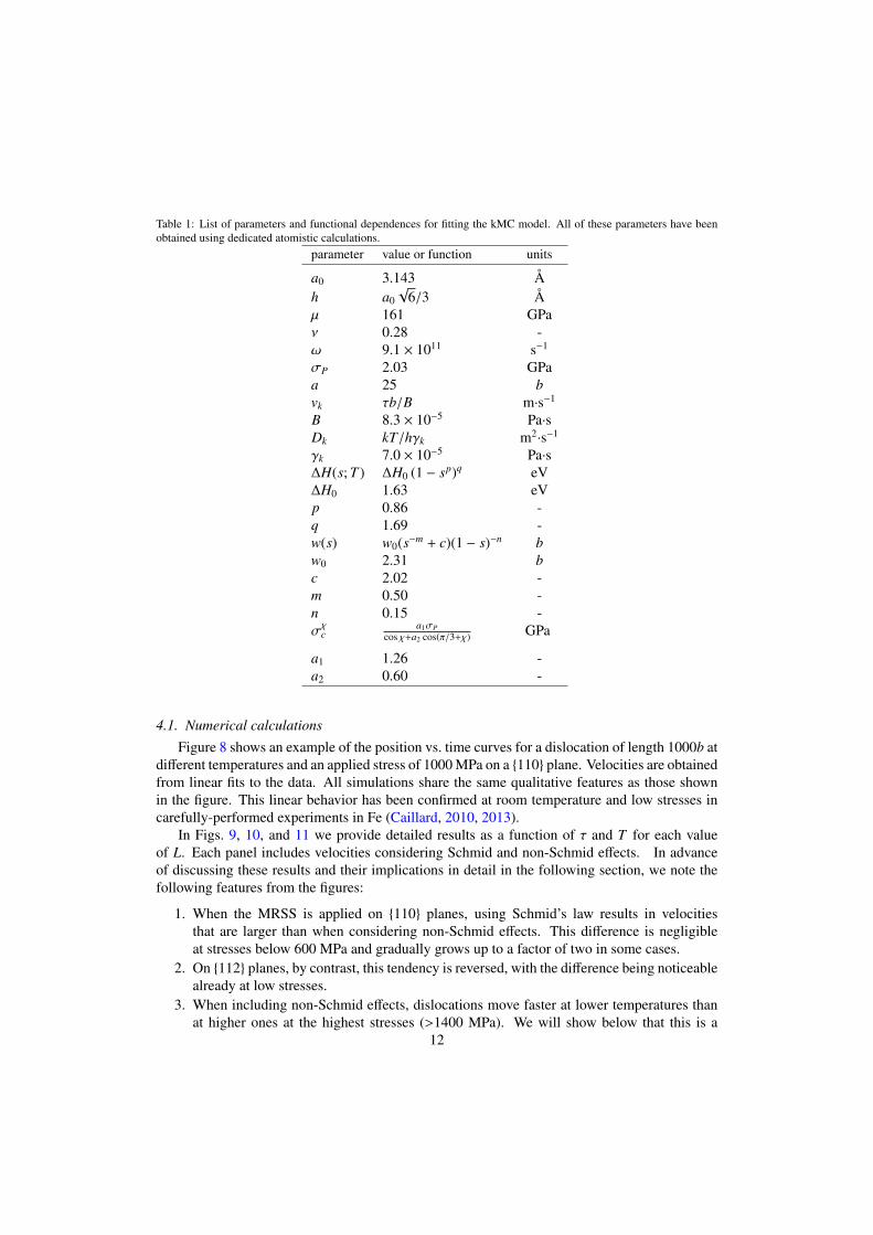
Table 1: List of parameters and functional dependences for fitting the kMC model. All of these parameters have beenobtained using dedicated atomistic calculations.
parameter value or function units
a0 3.143 Åh a0
√6/3 Å
µ 161 GPaν 0.28 -ω 9.1 × 10¹¹ s−1
σP 2.03 GPaa 25 bvk τb/B m·s−1
B 8.3 × 10⁻⁵ Pa·sDk kT/hγk m2·s−1
γk 7.0 × 10⁻⁵ Pa·s∆H(s; T ) ∆H0 (1 − sp)q eV∆H0 1.63 eVp 0.86 -q 1.69 -w(s) w0(s−m + c)(1 − s)−n bw0 2.31 bc 2.02 -m 0.50 -n 0.15 -σχc
a1σPcos χ+a2 cos(π/3+χ) GPa
a1 1.26 -a2 0.60 -
4.1. Numerical calculationsFigure 8 shows an example of the position vs. time curves for a dislocation of length 1000b at
different temperatures and an applied stress of 1000 MPa on a 110 plane. Velocities are obtainedfrom linear fits to the data. All simulations share the same qualitative features as those shownin the figure. This linear behavior has been confirmed at room temperature and low stresses incarefully-performed experiments in Fe (Caillard, 2010, 2013).
In Figs. 9, 10, and 11 we provide detailed results as a function of τ and T for each valueof L. Each panel includes velocities considering Schmid and non-Schmid effects. In advanceof discussing these results and their implications in detail in the following section, we note thefollowing features from the figures:
1. When the MRSS is applied on 110 planes, using Schmid’s law results in velocitiesthat are larger than when considering non-Schmid effects. This difference is negligibleat stresses below 600 MPa and gradually grows up to a factor of two in some cases.
2. On 112 planes, by contrast, this tendency is reversed, with the difference being noticeablealready at low stresses.
3. When including non-Schmid effects, dislocations move faster at lower temperatures thanat higher ones at the highest stresses (>1400 MPa). We will show below that this is a
12

consequence of self-pinning, which is favored in that regime. Using Schmid’s law, thistendency is observed in some selected cases, but not generally.
4. At high stresses, there are no appreciable differences between the velocity response forL = 100b, L = 1000b, and L = 4000b lines. A detailed investigation of the lengthdependence of the dislocation velocity will be conducted below.
4.2. Dislocation length dependence
It has been traditionally assumed that screw dislocation velocity depends linearly on itslength, a dependence introduced by construction in dislocation dynamics models (Tang et al.,1998; Naamane et al., 2010) but also confirmed experimentally in some limited cases at roomtemperatures and low stresses (Caillard, 2010, 2013). Here we perform a systematic study ofdislocation velocity as a function of L at several temperatures and stresses, and for Schmid andnon-Schmid conditions. First we study nominally the same regime as in the experimental worksby Caillard, i.e. room temperature (300 K) and low stress (200 MPa). We present results for thetwo slip systems of interest in Figure 12, where the linear dependency is clearly distinguished.This is a direct consequence of the form of eq. 3, when nucleation is the rate-limiting step andthe dynamics is governed by the existence of one single kink-pair on the line at a given time,i.e. li ≡ L. This is the expected behavior at low strain rates or in quasistastic conditions.
However, as the stress and/or the temperature increase, this trend becomes gradually weak-ened until it is lost altogether. Figure 13 shows results for τ = 1000 MPa at different temper-atures. In this situation, multiple kink-pairs may coexist at once, giving rise to cross-kinks andother self-pinning features that remove the linear dependence on L. These are the conditions thatare representative of high-strain rate situations.
4.3. Trajectory
Next we analyze the impact of considering non-Schmid effects on the trajectory of a screwdislocation projected on the [111] plane. Figure 14(a) shows an example at 300 K and 200 MPawhere the MRSS is on the (110) plane (for this analysis we use the axes convention given inFig. 1). As the figure shows, considering non-Schmid effects results only in a slight deviationfrom the MRSS plane, characterized by sporadic slip episodes on the (101) forming +60 withthe MRSS plane. More revealing is perhaps the case of glide when the MRSS is resolved on a112 plane –(211)T to be precise–. In this case, Schmid behavior is generally recovered wheneq. 2 is used, as Fig. 14(a) illustrates. The trajectory in this case follows a zig-zag pattern,characteristic of wavy slip observed in bcc systems at low temperature (e.g. Franciosi (1983)).However, non-Schmid behavior results in effective glide on the (101) plane, forming +30 withthe MRSS plane. This behavior is not inconsistent with recent Laue diffraction experiments ofslip in W (Marichal et al., 2013) and with MD simulations performed with the same potentialemployed here by Cereceda et al. (2013).
At higher stresses and temperatures (cf. Fig.14(b)) the same general behavior can be ob-served, although the deviation from the MRSS plane for non-Schmid 110 loading is morenotable than under low stress/temperature conditions. In all cases, deviations from the MRSSplane are reliably in a counterclockwise direction. This is a direct manifestation of the twinning-antitwinning asymmetry that biases kink-pair nucleation toward planes that are consistent withthe critical stresses shown in Fig. 7.
13

4.4. Dislocation self-pinningThe reason for the loss of linearity in the v-L dependence at high temperature or stress (Figs.
13(a) and 13(b)) is related to the increased probability of forming kink pairs on multiple glideplanes simultaneously. According to equation 3, this probability increases with temperature,stress, and line length, consistent with the behavior discussed above. As alluded to in Section2.2, in multislip conditions the interaction among kink pairs on different planes results in crosskinks. These defects essentially halt the progress of the dislocation by acting as pinning pointsthat must be overcome before motion can resume. When this happens, debris loops are formedin the wake of the main dislocation. Figure 15 shows the final configuration after 5000 kMCcycles of a screw dislocation of length L = 1000b under 112-Schmid loading at 1000 MPa anda temperature of 1800 K. The figure clearly shows trailing chains of debris loops. The readeris referred to the work by Marian et al. (2004) for more details on the atomistic characteristicsof this process. Here we quantify the formation of these loops and relate it to dislocation self-pinning and slowing down.
From analysis of trajectories such as that shown in Fig. 15, the number of debris loops perunit time per unit length can be tallied as a function of τ, T , L, and MRSS plane. This debrisloop generation rate –which we term γ– is shown in Figure 16 for 112 non-Schmid loading fora dislocation with L = 4000b. As expected, γ increases with increasing temperature and stress.However, for a given temperature and glide condition, the loop generation rate per unit length isindependent of L. This is illustrated in Figure 17, where γ is shown as a function of stress for112 non-Schmid conditions and at 900 K for L = 100, 1000, and 4000b. In other words, thedebris loop generation rate only depends on temperature, stress, and the glide condition. Theexample shown here is representative of other temperatures and MRSS plane orientations.
These results show that there may be a correlation between the degree of self-pinning in Figs.9, 10, and 11 and the value of γ for each case. For the specific example shown in Fig. 17, Fig.11(b) suggests that the dislocation velocity deviates from the nominal exponential behavior at astress of ≈1500 MPa. This corresponds to a value of γ = 1.5×10⁸ s−1 b−1 (the approximate valueof the three curves in Fig. 17 at 1500 MPa). This apparent threshold is of course temperature de-pendent and varies with loading orientation, although here we only consider the case showcasedin Figs. 16 and 17.
4.5. Computational efficiencyAs discussed in the previous section, the compounded effect of stress, temperature, and initial
screw dislocation length, as well as stress orientation, is to enhance the probability to nucleatekink-pairs in multiple slip planes. This increases the number of segments and may lead to astalled kinetic evolution as a consequence of self-pinning. Both of these phenomena decreasethe computational efficiency of the kMC code, interpreted as the utilization of CPU time to resultin net dislocation motion. The number of segments increases the numerical workload of theO(N2) segment-segment stress calculation function5, while self-pinning arrests the dislocationprogress resulting in slower net motion. To assess these overhead costs quantitatively, we plot inFigure 18 the dependence of the computational efficiency η as a function of applied RSS and L.The calculations were performed for a fixed number of 2000 kMC cycles at 900 K. For claritywe display η in arbitrary units to showcase the effect of each parameter studied, with quantitativedetails about the numerical values in each case given in Appendix C. As shown in the figure,
5Profiling tests reveal that > 92% of the CPU time in any given kMC cycle is spent in this function.14

increasing the stress, the dislocation line length, and/or under 112 loading, all contribute toefficiency losses. Stress and temperature are generally equivalent in their effect on η, and so hereonly the impact of τ is evaluated.
5. Discussion
Motivation for using kMC simulations – The motion of screw dislocations proceeds via thethermally-activated nucleation of kink-pairs and kink propagation along the screw direction.Kinks are atomistic entities –as described in Figure 4– but also elastic ones. This means thattheir properties must be characterized at the atomistic scale, but their effects can be potentiallylong-ranged. Dynamically, by virtue of its rare-event nature, kink pair nucleation operates ontime scales that are hardly accessible by atomistic methods. This precludes, in most cases theuse of direct MD or other atomistic methods. However, dislocations containing kink pairs aresubjected to long-range elastic self-forces, which have to be integrated along the dislocation inorder to be evaluated and resolved spatially. As this is typically very numerically-intensive, weresort to discretization methods that treat dislocation lines as piece-wise entities in which allsegments interact with all segments. This, for its part, precludes the use of effective-mediummethodologies such as the line-tension approximation or other techniques in which these O(N2)interactions are not captured. KMC, in our mind, offers the ideal alternative to bridge these twolimits. On the one hand, the dislocation is treated as a piece-wise object attached to an under-lying lattice. This allows us to represent some of the most important atomistic features of thedislocation fairly accurately. At the same time, this piece-wise representation enables the cal-culation of all the elastic forces in an efficient manner. The result is a method that can accesstime scales long enough to statistically capture dislocation motion, yet it retains sufficient detailto accurately provide a clear connection to the underlying atomistic physical features.
Comparison with MD results – One of the main motivations behind the development of ourkMC model was MD’s inability to sample thermally activated motion within its space and timelimitations. It is then useful to compare MD and kMC results of screw dislocation glide subjectedto nominally identical boundary conditions. However, as discussed above, the overdriven natureof MD simulations causes the occurrence of cross-kinks and associated debris for line lengths forwhich the kMC simulations predict smooth glide. This is illustrated in Figure 19, where a screwdislocation of length 100b is seen to leave vacancy clusters behind at 300 K and 1100 MPa ofstress applied on a 112 plane. For the current interatomic potential, the threshold length belowwhich cross kinks are not seen to occur was estimated to be 25b (Cereceda et al., 2013). Thisis below the length for which kMC simulations can support an elementary kink pair. Therefore,we are forced to make an imperfect comparison between the MD results with L = 25b and thekMC results for L = 75b, which is near the minimum length in kMC calculations to contain onekink-pair.
Results from both approaches are shown in Figure 20. The figure shows that the MD veloc-ities are systematically higher than their kMC counterparts below 1500 MPa. Above this value,the kMC velocities at 300 and 600 K overtake the MD-calculated values. It is interesting to notethat the qualitative shape of the MD curves coincides with those of the kMC curves at the highesttemperatures of 1200 and 1800 K. This is symptomatic of the limitations of MD, which evenat low stresses and temperatures create simulation conditions that are representative of highervalues. It must also be kept in mind that a sensitivity study has not been conducted on the kMCparameters, and thus the present comparison is only valid inasmuch as the current parameter-ization can be considered a sufficiently valid one for the method. In terms of computational
15

overhead, MD simulations are approximately three to seven orders of magnitude costlier thantheir kMC counterparts on the basis of the metric employed in Table C.3. We refer the reader toAppendix C for more details.
Dislocation self-pinning – Self-pinning occurs as a consequence of the formation of cross-kinks, which act as strong sessile junctions. Cross-kinks may be resolved topologically by com-plementary kink pairs, resulting in the closing of a debris loop behind. Loop generation con-tributes to self-pinning as well. The energy expended in producing debris loops is taken outof the total mechanical work available to make the dislocation glide, which results in an effec-tive ‘reduced’ stress and, therefore, lower velocities. Physically, self-pinning is seen to becomeimportant above a certain generation rate threshold, which correlates with a leveling-off of dis-location velocity curves as a function of stress.
This notion of threshold generation rate originates in the creation of kink-pairs on multipleslip planes, whose effect in the kinetic behavior depends on the combined effects of cross-kinkproduction and resolution. An enhanced probability of kink pair production (brought about byincreasing temperature, stress, and/or multislip conditions) may facilitate the production of cross-kinks, leading to potentially higher self-pinning. At the same time, the probability for resolutionof these is also intensified by the same processes. Resolution of cross kinks results in debrisloop production. Beyond the apparent debris generation threshold, however, the production ofcross-kinks overruns the likelihood of resolution, effectively arresting the dislocation progressand stagnating the velocity increase with temperature and stress. When this happens, debris pro-duction is simply a manifestation of self-pinning on the larger scale. This is one of the reasonsleading to the length independent behavior observed at mid-to-high temperatures and stresses(cf. Fig. 13), and which is behind the anomalous behavior of some dislocations observed experi-mentally (Hsiung, 2007).
Extraction of effective mobility laws – Ultimately, the data compiled in this work via extensivekMC calculations must be used to fit mobility functions suitable for, e.g. dislocation dynamics,phase field, or crystal plasticity simulations (see for example Tang & Marian (2014)). The de-viations exposed by our calculations from the expected exponential behavior due to self-pinningcall for a possible fitting function of the following type:
v(s,T ) = A′sn′ f ′(s,T )(1 − B′ f ′(s,T )
)(9)
f ′(s,T ) = exp−
∆H0
kT
(1 − sp′
)q′
where A′, B′, n′, p′, and q′ are all adjustable parameters and s is defined as in eq. 2 or B.4.The above expression captures the leveling-off displayed in the v-τ relations at high stress andtemperature. By way of example, here we fit the results for L = 4000b. Table 2 gives the param-eters under each specific glide condition. Figure 21 shows the fit for non-Schmid conditions ona 112 plane. The agreement between the fitting functions and the data is similar for other glideconditions and/or values of L.
Limitations of the method – We conclude this section discussing some of the limitations ofour model. First, the sampling function 3 contains several parameters with exponential depen-dence that have been obtained via atomistic calculations using a recent interatomic potential. Assuch, they are subjected to errors associated with the atomistic technique used (NEB), the typeof potential and its parameterization (EAM), and the least-squares fitting procedure. In a way,all these errors are unavoidable –in the sense that we have employed ‘state-of-the-art’ techniquesand procedures– but their impact on the overall kinetics, although unassessed at the moment,
16

Table 2: Adjustable parameters for the fitting function given in eq. 9. The units of A′ are such that v(s,T ) is in m·s−1,i.e. m·s−1·MPa−n. All other parameters are non-dimensional.
Temperature range [K] A′ n′ B′ p′ q′
110 Schmid loadingAll temperatures 3693.4 2.47 0.97 0.16 1.00
110 Non-Schmid loading300 698.2 0.30 0.0 1.15 2.97> 300 1444.2 1.78 0.72 0.26 1.40
112 Schmid loadingAll temperatures 755.6 0.38 0.50 0.22 1.01
112 Non-Schmid loading≤ 600 2084.2 1.39 0.68 0.81 2.45> 600 3416 2.72 0.89 0.19 1.32
might conceivably be notable in some cases. Next, the very physical foundation of the code–the Arrhenius expression for the thermally activated kink-pair nucleation rate– may be calledinto question under some of the conditions explored here. Indeed, at high stresses (and tempera-tures) the kinetics is better represented by generalized Arrhenius forms, e.g. the Jackson formula(Swinburne, 2013), and this may affect the high stress/temperature tails of the velocity-stressrelations given in Figs. 9, 10, and 11. The representation of dislocation segments may also be asource of errors in our setting. Kinks and screw segments are joined by sharp corners that giverise to stress singularities –these are avoided here by resorting to a screening distance withinwhich the stress is not calculated– that are artifacts of our piecewise rectilinear representation ofdislocation lines. Another physical phenomenon not captured in these simulations is the soften-ing of the elastic constants and Peierls (critical) stress with temperature. In particular, today’scomputational resources permit the direct calculation of the temperature dependence of the crit-ical stress (Gilbert et al., 2013). It is not clear at his point how significant this dependence ison the dislocation velocities calculated here. Finally, it is worth mentioning that the impact ondislocation motion of non-glide stresses –another source of non-Schmid effects– is not presentlyconsidered in this work, although its implementation is straightforward if the data were available.
6. Summary
We have developed a kinetic Monte Carlo model of thermally-activated screw dislocationmotion in bcc crystals, with a current parameterization for W using a state-of-the-art interatomicpotential. Our method includes all relevant physical processes attendant to screw dislocationmotion, including –for the first time– kink diffusion and non-Schmid effects.
With the versatility and efficiency afforded by our kMC algorithm, we have studied disloca-tion mobility as a function of stress, temperature, initial dislocation line length, and MRSS planeorientation. An attractive feature of the present calculations is that they allow us to separateimportant mobility dependencies and assess their impact on the kinetics individually.
We find that non-Schmid effects have an important influence on the absolute value of the ve-locity as function of both stress and temperature, suggesting that they cannot be neglected in plas-ticity simulations. We also find that at sufficiently high stresses and temperatures, self-pinningprocesses control dislocation motion. Finally, some effective fitting functions are proposed that
17

capture the essential features of dislocation motion to be used in more homogenized models ofcrystal deformation.
Acknowledgments
We are indebted to V. Bulatov for useful discussions and helpful guidance. Conversationswith D. Rodney, M. Gilbert, and W. Cai are gratefully acknowledged. This work was performedunder the auspices of the U.S. Department of Energy by Lawrence Livermore National Labora-tory under Contract No. DE-AC52-07NA27344. J. M. acknowledges support from DOE’s EarlyCareer Research Program. D. C. acknowledges support from the Consejo Social and the PhDprogram of the Universidad Politécnica de Madrid. T. D. S. was supported through a studentshipin the Centre for Doctoral Training on Theory and Simulation of Materials at Imperial CollegeLondon funded by EPSRC under Grant No. EP/G036888/1. This work was part-funded bythe RCUK Energy Programme (Grant Number EP/I501045) and by the European Union’s Hori-zon 2020 research and innovation programme. The views and opinions expressed herein do notnecessarily reflect those of the European Commission. This work was also part-funded by theUnited Kingdom Engineering and Physical Sciences Research Council via a programme grantEP/G050031.
18

−20
−15
−10
−5
0
5
10
0.0 0.2 0.4 0.6 0.8 1.0
H [e
V]
Reaction coordinate [a0√6/3]
0 MPa100 MPa
200 MPa300 MPa400 MPa
500 MPa600 MPa700 MPa800 MPa
900 MPa1000 MPa1100 MPa
1200 MPa1300 MPa1400 MPa
1500 MPa1600 MPa
Peierls path
Figure 5: NEB transition pathway along the Peierls coordinate for screw dislocation segments of length 100b. The acti-vated state is taken as the point of maximum enthalpy in each case, where the kink pair separation is measured. The insetscorrespond to kink pair configurations at several points along the NEB trajectory visualized using the centrosymmetrydeviation parameter.
19

0.0
0.5
1.0
1.5
2.0
0.0 0.2 0.4 0.6 0.8 1.0
Kin
k pa
ir en
thal
py [e
V]
s
∆H0 = 1.63 eVp = 0.86q = 1.69
∆H(s)=∆H0(1−sp)q
Atomistic data
(a)
0
10
20
30
40
50
60
0.0 0.2 0.4 0.6 0.8 1.0
Kin
k pa
ir se
para
tion
[b]
s
w0 = 2.31b
m = 0.50c = 2.02n = 0.15
w(s)=w0(s−m +c)(1−s)−n
Atomistic data
(b)
Figure 6: Kink pair activation enthalpy and separation as a function of stress. The data in each case are fitted to eqs. 4and 5, with the resulting fitting parameters shown in each case.
20

(121)AT
[111] (110)
(211)T
+χ-χ
Stress
[σ P]
0.0
0.5
1.0
1.5EAM data
Schmid lawNon-Schmid fit
Figure 7: Dependence of the critical resolved shear stress with the angle between the MRSS plane and the primary glideplane. The standard Schmid law is shown as a vertical green-colored line.
21

0
50
100
150
200
250
300
350
400
450
0 1 2 3 4 5 6 7 8
Pos
ition
[×10
−10
m]
Time [×10−10 s]
L=1000b
110 glideσ = 1000 MPa
300 K600 K900 K
1200 K1800 K
0.0
0.2
0.4
0 5 10 15
Figure 8: Average dislocation position vs. time at different temperatures for L = 1000b with a RSS of 1000 MPa on a110 plane. These simulations were carried out including non-Schmid effects. Due to differences in scale, the trajectoryat 300 K is shown separately in the inset.
22

0
100
200
300
400
500
600
0 500 1000 1500 2000
velo
city
[m⋅s
-1]
τ [MPa]
L=100b
110 glide
300K600K900K
1200K1800K
SchmidNon-Schmid
(a) L = 100b, 110 loading
0
100
200
300
400
500
600
0 500 1000 1500 2000
velo
city
[m⋅s
-1]
τ [MPa]
L=100b
112 glide
300K600K900K
1200K1800K
SchmidNon-Schmid
(b) L = 100b, 112 loading
Figure 9: Velocity-stress relations for L = 100b for all temperatures, stresses, and including Schmid and non-Schmidloading.
23

0
100
200
300
400
500
600
0 500 1000 1500 2000
velo
city
[m⋅s
-1]
τ [MPa]
L=1000b
110 glide
300K600K900K
1200K1800K
SchmidNon-Schmid
(a) L = 1000b, 110 loading
0
100
200
300
400
500
600
0 500 1000 1500 2000
velo
city
[m⋅s
-1]
τ [MPa]
L=1000b
112 glide
300K600K900K
1200K1800K
SchmidNon-Schmid
(b) L = 1000b, 112 loading
Figure 10: Velocity-stress relations for L = 1000b for all temperatures, stresses, and including Schmid and non-Schmidloading.
24

0
100
200
300
400
500
600
700
0 500 1000 1500 2000
velo
city
[m⋅s
-1]
τ [MPa]
L=4000b 110 glide
300K600K900K
1200K1800K
SchmidNon-Schmid
(a) L = 4000b, 110 loading
0
100
200
300
400
500
600
700
0 500 1000 1500 2000
velo
city
[m⋅s
-1]
τ [MPa]
L=4000b 112 glide
300K600K900K
1200K1800K
SchmidNon-Schmid
(b) L = 4000b, 112 loading
Figure 11: Velocity-stress relations for L = 4000b for all temperatures, stresses, and including Schmid and non-Schmidloading.
25

0.0
0.2
0.4
0.6
0.8
1.0
1.2
1.4
0 500 1000 1500 2000 2500 3000 3500 4000
velo
city
[×10
−15
m⋅s
−1 ]
L [b]
T = 300 Kσ = 200 MPa
110 Schmid110 Non−Schmid
112 Schmid112 Non−Schmid
Figure 12: Dependence of the dislocation velocity on its initial length for a resolved shear stress of 200 MPa at 300 Kand under Schmid and non-Schmid conditions.
26

0
50
100
150
200
0 500 1000 1500 2000 2500 3000 3500 4000
velo
city
[m⋅s
−1 ]
L [b]
600K900K
1200K
1800KSchmid
Non−Schmid
(a) τ = 1000 MPa, 110 loading
0
50
100
150
200
0 500 1000 1500 2000 2500 3000 3500 4000
velo
city
[m⋅s
−1 ]
L [b]
600K900K
1200K
1800KSchmid
Non−Schmid
(b) τ = 1000 MPa, 112 loading
Figure 13: Dependence of the dislocation velocity on its initial length for a resolved shear stress of 1000 MPa at hightemperatures and under Schmid and non-Schmid conditions.
27

0
50
100
150
0 50 100 150 200 250
y [b
]
x [b]
(110)
(211) T
(101
)
−
−−
−
−−
−
(110) Schmid(110) Non−Schmid
(211) Schmid(211) Non−Schmid
(a) T = 300 K and τ = 200 MPa.
−5
0
5
10
15
20
25
0 5 10 15 20 25 30 35 40
y [b
]
x [b]
(110)
(211) T
(101
)
−
−−
−
−−
−
(110) Schmid(110) Non−Schmid
(211) Schmid(211) Non−Schmid
(b) T = 1800 K and τ = 1000 MPa.
Figure 14: Trajectory of a dislocation line of length L = 4000b under Schmid and non-Schmid conditions.
28

(211) plane
Connected dislocation
L
Figure 15: Final configuration after 5000 kMC cycles of a screw dislocation of length L = 1000b under 112-Schmidloading conditions at 1000 MPa and a temperature of 1800 K. Segments in dark blue belong to the main dislocation,while colored segments belong to detached loops. The depicted line configuration is scaled in the z direction to facilitateviewing. See the Supplementary animation of the time evolution of the dislocation.
29

0
5
10
15
20
0 200 400 600 800 1000 1200 1400 1600 1800
γ [×
108 b
−1 ⋅s
−1 ]
τ [MPa]
.
112 non−Schmid glide
L=4000b
300 K600 K900 K
1200 K1800 K
Figure 16: Debris loop generation rate as a function of temperature and applied stress for 112 non-Schmid conditionsfor a dislocation with L = 4000b. At 300 K there is zero loop generation.
0.0
0.5
1.0
1.5
2.0
2.5
3.0
3.5
4.0
0 200 400 600 800 1000 1200 1400 1600 1800
γ [×
108 b
−1 ⋅s
−1 ]
τ [MPa]
.
112 non−Schmid glideT=900 K
Apparent threshold
L=100b
L=1000b
L=4000b
Figure 17: Debris loop generation rate at 900 K during 112 non-Schmid conditions for three different initial dislocationlengths. The apparent threshold above which self-pinning is seen to dominate the kinetics is marked with a dashed line.
30

0 200 400 600 800 1000
400
800
1200
η
110 MRSS plane 112 MRSS plane
L [b]σ [MPa]
η
Figure 18: Computational efficiency η measured in arbitrary units as a function of L, τ, and MRSS plane for a number ofsimulations conducted at 900 K for a fixed duration of 2000 kMC cycles.
31

Figure 19: MD simulation of a screw dislocation under the following conditions: L = 100b, T = 300 K, σRSS = 1100MPa, MRSS plane ≡ 112. After a few time steps, the dislocation starts producing debris in the form of vacancy andinterstitial clusters. These are akin to small dislocation loops in he kMC simulations.
0
100
200
300
400
500
600
0 500 1000 1500 2000
velo
city
[m⋅s
-1]
τ [MPa]
112 glide 300K600K900K
1200K1800K
Non-Schmid kMCMD
Figure 20: Comparison of dislocation velocities from MD results (Cereceda et al., 2013) and kMC calculations.
32

0
100
200
300
400
500
600
700
0 200 400 600 800 1000 1200 1400 1600 1800
velo
city
[m⋅s
−1 ]
τ [MPa]
L=4000b
112 non−Schmid glide
300K600K900K
1200K1800K
Figure 21: Comparison between eq. 9 (solid lines) parameterized for L = 4000b under non-Schmid 112 glide conditionsand the actual kMC data.
33

Appendix A. Computing diffusion and drift coefficients of isolated single kinks
To generate isolated kinks in an MD supercell, we use especial boundary conditions that en-force a tilt equal to a lattice vector k. Depending on the value of k kinks of opposite signs –‘right’and ‘left’, to employ the usual convention– are created in cells containing a balanced dislocationdipole. These configurations are then equilibrated at finite temperature and the simulation outputis then time averaged and energy filtered in both zero and finite stress conditions to produce aseries of kink positions x from which a kink drift and diffusivity can be statistically determined.This procedure is described in detail by Swinburne et al. (Swinburne et al., 2013), and a typicalsimulation supercell (containing around 106 atoms) is depicted in Figure A.22.
Figure A.22: Illustration of kink drift simulations. Kinks on a 1/2〈111〉101 screw dislocation dipole, characterized bya lattice ‘kink’ vector k, are subject to an applied stress on bounding (101) planes. Under no applied stress with fullyperiodic boundary conditions the kinks diffuse freely. Inset: Cartoon of the supercell along [101], illustrating the relationof the kink vector to a kinked dislocation line.
The results of these simulations are displayed in Figure A.23. Kinks were observed to freelydiffuse with a diffusivity D = kT/B under no applied stress with fully periodic boundary con-ditions, while, under stresses of 2∼10 MPa applied to the bounding (101) planes, kinks wereobserved to drift with a viscous drag law x = |σ · b|/B. Although the two screw dislocationseventually annihilate under applied stress, for a sufficiently wide and long supercell, the kinksdrift independently for at least two supercell lengths (∼600 Å) before any influence of their mu-tual attraction can be detected.
The drift and diffusion simulations are fitted to the Einstein relation:
D = kT lim|σ·b|→0
x|σ · b|
whereupon it is seen that the viscous drag B is independent of temperature and shows littlevariation between left and right kinks. The final mobility laws were determined to be vk =
34

0
50
100
150
200
250
300
0 100 200 300 400 500 600
Kin
k P
ositi
on [
A]
Time [ps]
T = 30K, 60K,120K, 180K
Kink velocity = | b|/B
| | = 10 M
Pa
| | = 2 MPa
04
8
12
16 D=kT/B
0 60 120 180 240
D [
A2 /p
s]
T [K]
Left k=[010]
Right k=1/2[111]_
Figure A.23: Results of kink drift simulations for k = 1/2[111] (right) kinks on 1/2〈111〉101 screw dislocations. We seea temperature independent drift velocity vk = |σ · b|/B in very good agreement with B determined from zero stress kinkdiffusion simulations (green lines). Inset: Results from kink diffusion simulations. We see the diffusivity D = kT/B riseslinearly with temperature, meaning that B is independent of temperature.
3.8×10⁻⁶τ for k = 1/2[111] (‘right’ or ‘interstitial’) kinks and vk = 4.0×10⁻⁶τ for k = [010] (‘left’or ‘vacancy’) kinks. These velocities are in m·s−1 when the stress is in Pa. Phonon scatteringtreatments (Hirth & Lothe, 1991) predict that B should increase linearly with temperature dueto the increased phonon population, but the observed temperature independence of B agreeswith previous studies of kink diffusion (Swinburne et al., 2013) and other nanoscale defects(Dudarev, 2008). The assumption of constant kink velocity is justified on the basis of the energylandscape over which kinks move. This landscape is effectively flat –albeit with significantthermal roughness– due to the onset of vibrational chaos, which destroys inertial motion andleaves linear viscous motion as the dominant one. Potentially, at very low temperatures and highstresses this regime could break down and be replaced by one where inertial effects are dominant.However, we have not contemplated this possibility.
Appendix B. Implementing non-Schmid effects in the kinetic Monte Carlo calculations
In the reference system used in Fig. 1, the MRSS is unequivocally defined as:
σMRSS =
√σ2
xz + σ2yz
35

with
θMRSS = arctan(−σxz
σyz
)and
χ = θMRSS − θ
For the purpose of the implementation of non-Schmid effects, we express eq. 2 in terms of theMRSS by noting that, from Fig. 1, σRSS = σMRSS cos χ:
s(χ) =σMRSS cos χ
σP(B.1)
Schmid law states that the critical stress σc(χ) depends on χ as:
σc(χ) =σP
cos χ(B.2)
which results in rewriting eq. 2 as:s(χ) =
σMRSS
σc(χ)(B.3)
Proving that eqs. 2 and B.3 are equivalent is straightforward:
σRSS = σMRSS cos χ= σMRSS cos(θMRSS − θ)= σMRSS [sin θMRSS sin θ + cos θMRSS cos θ]= σMRSS sin θMRSS sin θ + σMRSS cos θMRSS cos θ= −σxz sin θ + σyz cos θ
From this, non-Schmid effects are introduced by substituting the following expression:
σc(χ) =a1σP
cos χ + a2 cos (π/3 + χ)
into eq. B.3:
s(χ) =σMRSS
σc(χ)=σMRSS (cos χ + a2 cos (π/3 + χ))
a1σP(B.4)
whence it is readily seen that Schmid behavior is recovered for a1 = 1 and a2 = 0. Figure B.24showcases the difference between s(χ) for Schmid and non-Schmid behavior as a function of θ.
Appendix C. Computational efficiency
The computational efficiency is assessed in the following manner. For the purposes of thispaper, we assume that the productivity of a kMC run is based on the distance traveled by a dislo-cation during a fixed number of cycles, as a longer distance results in better converged velocitycalculations and more precise data. Our performance metric of choice is then to normalize thedistance traveled in each case by the CPU time invested in achieving it. Table C.3 gives thenumerical values for this metric in Å per second of CPU time for various dislocation lengths andapplied stresses. These data are the basis for what is shown in Fig. 18.
36

Non−SchmidSchmid
−90 −60 −30 0 30 60 90
θMRSS [°]−90−60
−300
3060
90
θ [°]
−1.5
−1.0
−0.5
0.0
0.5
1.0
1.5
s
Figure B.24: Comparison between the normalized stress s under Schmid and non-Schmid conditions as a function of θand θMRSS. Recall that χ = θMRSS − θ.
As a point of comparison with ‘equivalent’6 MD simulations, we first resort to the data pub-lished by Cereceda et al. (2012), where the nominal cost of one time step per atom is ≈ 1.5×10⁻⁵
CPU seconds for the interatomic potential employed here. For 750,000 atoms, that is 11.25 CPUs per time step. Typical MD simulations involve 105 steps of 1 fs each, which results in 1.12×10⁶
CPU seconds. Again, per the data in ref. (Cereceda et al., 2012), those simulations achieve dis-placements on the order of 850 Å, which results in 7.5×10⁻⁴ Å per CPU second. This representsefficiencies of three to seven orders of magnitude lower than our kMC simulations.
References
Ariza, M. P., Tellechea, E., Menguiano, A. S., & Ortiz, M. (2012). Double kink mechanisms for discrete dislocations inBCC crystals. International Journal of Fracture, 174, 29–40.
Barvinschi, B., Proville, L., & Rodney, D. (2014). Quantum Peierls stress of straight and kinked dislocations and effectof non-glide stresses. Modelling and Simulation in Materials Science and Engineering, 22, 025006.
Bulatov, V. V., Richmond, O., & Glazov, M. V. (1999). An atomistic dislocation mechanism of pressure-dependentplastic flow in aluminum. Acta Materialia, 47, 3507–3514.
Cai, W., Arsenlis, A., Weinberger, C. R., & Bulatov, V. V. (2006). A non-singular continuum theory of dislocations.Journal of the Mechanics and Physics of Solids, 54, 561–587.
Cai, W., Bulatov, V. V., Justo, J. F., Argon, A. S., & Yip, S. (2002). Kinetic Monte Carlo approach to modeling dislocationmobility. Computational Materials Science, 23, 124–130.
6In the sense that they are designed to measure similar properties.37

Table C.3: Numerical values in Å per CPU second of the efficiency metric considered to evaluate the kMC code’sperformance under different conditions.
τ = 400 MPa, T = 900 K, 2000 kMC stepsL 100b 200b 500b 1000b
110MRSS plane 1180 634 267 113112MRSS plane 640 534 209 88
τ = 800 MPa, T = 900 K, 2000 kMC stepsL 100b 200b 500b 1000b
110MRSS plane 921 219 20.0 2.7112MRSS plane 150 23.0 1.0 -
τ = 1200 MPa, T = 900 K, 2000 kMC stepsL 100b 200b 500b 1000b
110MRSS plane 267 34.7 2.0 0.21112MRSS plane 8.3 1.7 - -
Cai, W., Bulatov, V. V., Yip, S., & Argon, A. S. (2001). Kinetic Monte Carlo modeling of dislocation motion in BCCmetals. Materials Science and Engineering: A, 309-310, 270–273.
Caillard, D. (2010). Kinetics of dislocations in pure Fe. Part I. In situ straining experiments at room temperature. ActaMaterialia, 58, 3493–3503.
Caillard, D. (2013). A TEM in situ study of alloying effects in iron. I-Solid solution softening caused by low concentra-tions of Ni, Si and Cr. Acta Materialia, 61, 2793–2807.
Cereceda, D., Perlado, J. M., & Marian, J. (2012). Techniques to accelerate convergence of stress-controlled moleculardynamics simulations of dislocation motion. Computational Materials Science , 62, 272–275.
Cereceda, D., Stukowski, A., Gilbert, M. R., Queyreau, S., Ventelon, L., Marinica, M.-C., Perlado, J. M., & Marian,J. (2013). Assessment of interatomic potentials for atomistic analysis of static and dynamic properties of screwdislocations in W. Journal of Physics: Condensed Matter, 25, 085702.
Chaussidon, J., Fivel, M., & Rodney, D. (2006). The glide of screw dislocations in bcc Fe: Atomistic static and dynamicsimulations. Acta Materialia, 54, 3407–3416.
Chen, Z. M., Mrovec, M., & Gumbsch, P. (2013). Atomistic aspects of 12 〈111〉 screw dislocation behavior in α-iron and
the derivation of microscopic yield criterion. Modelling and Simulation in Materials Science and Engineering, 21,055023.
Christian, J. W. (1983). Some surprising features of the plastic deformation of body-centered cubic metals and alloys.Metallurgical Transactions A, 14, 1237–1256.
Dao, M., Lee, B. J., & Asaro, R. J. (1996). Non-Schmid Effects on the Behavior of Polycrystals with Applications toNi3Al. Metallurgical and Materials Transactions A, 27A, 81.
Deo, C. S., & Srolovitz, D. J. (2002). First passage time Markov chain analysis of rare events for kinetic Monte Carlo:double kink nucleation during dislocation glide. Modelling and Simulation in Materials Science and Engineering, 10,581.
Dorn, J. E., & Rajnak, S. (1964). Nucleation of kink pairs and the Peierls mechanism of plastic deformation. Trans.Metall. Soc. AIME, 230, 1052.
Dudarev, S. L. (2008). The non-Arrhenius migration of interstitial defects in bcc transition metals. Comptes RendusPhysique, 9, 409 – 417. doi:10.1016/j.crhy.2007.09.019.
Duesbery, M. S., & Vitek, V. (1998). Plastic anisotropy in b.c.c. transition metals. Acta Materialia, 46, 1481–1492.Edagawa, K., Suzuki, T., & Takeuchi, S. (1997). Motion of a screw dislocation in a two-dimensional Peierls potential.
Physical Review B, 55, 6180.Franciosi, P. (1983). Glide mechanisms in b.c.c. crystals: An investigation of the case of ?-iron through multislip and
latent hardening tests. Acta Metallurgica, 31, 1331–1342.Gilbert, M. R., Queyreau, S. R., & Marian, J. (2011). Stress and temperature dependence of screw dislocation mobility
in α-Fe by molecular dynamics. Physical Review B, 84, 174103.Gilbert, M. R., Schuck, P. C., Sadigh, B., & Marian, J. (2013). Free Energy Generalization of the Peierls Potential in
Iron. Physical Review Letters, 111, 095502.Gordon, P. A., Neeraj, T., Li, Y., & Li, J. (2010). Screw dislocation mobility in BCC metals: the role of the compact core
on double-kink nucleation. Modelling and Simulation in Materials Science and Engineering, 18, 085008.
38

Gröger, R., & Vitek, V. (2005). Breakdown of the Schmid Law in BCC Molybdenum Related to the Effect of ShearStress Perpendicular to the Slip Direction. Materials Science Forum, 482, 123–126.
Hale, L. M., Zimmerman, J. A., & Weinberger, C. R. (2014). Simulations of bcc tantalum screw dislocations: Whyclassical inter-atomic potentials predict 112 slip. Computational Materials Science, 90, 106–115.
Hirth, J., & Lothe, J. (1991). Theory Of Dislocations. Malabar, FL Krieger.Hsiung, L. (2007). Dynamic Dislocation Mechanisms for the Anomalous Slip in a Single-Crystal BCC Metal Oriented
for “Single Slip”. Technical Report UCRL-TR-227296 Lawrence Livermore National Laboratory Livermore, CA.URL: https://e-reports-ext.llnl.gov/pdf/342520.pdf.
Ito, K., & Vitek, V. (2001). Atomistic study of non-Schmid effects in the plastic yielding of bcc metals. PhilosophicalMagazine A, 81, 1387–1407.
Kocks, U. F., Argon, A. S., & Asby, M. F. (1975). Thermodynamics and Kinetics of Slip. Progress in Materials Science,19, 1.
Koizumi, H., Kirchner, H. K. H., & Suzuki, T. (1993). Kink pair nucleation and critical shear stress. Acta Metallurgicaet Materialia, 41, 3483.
Lassner, E., & Schubert, W. F. (1999). Tungsten:Properties, Chemistry, Technology of the Element, Alloys, and ChemicalCompounds. New York: Kluwer.
Lim, H., Weinberger, C. R., Battaile, C. C., & Buchheit, T. E. (2013). Application of generalized non-Schmid yield law tolow-temperature plasticity in bcc transition metals. Modelling and Simulation in Materials Science and Engineering,21, 045015.
Lin, K., & Chrzan, D. C. (1999). Kinetic Monte Carlo simulation of dislocation dynamics. Physical Review B, 60, 3799.Marian, J., Cai, W., & Bulatov, V. V. (2004). Dynamic transitions from smooth to rough to twinning in dislocation
motion. Nature Materials, 3, 158–163.Marichal, M., Van Swygenhoven, H., Van Petegem, S., & Borca, C. (2013). 110 Slip with 112 slip traces in bcc
Tungsten. Scientific Reports, 3, 2547.Marinica, M.-C., Ventelon, L., Gilbert, M. R., Proville, L., Dudarev, S. L., Marian, J., Bencteux, G., & Willaime, F.
(2013). Interatomic potentials for modelling radiation defects and dislocations in tungsten. Journal of Physics:Condensed Matter, 25, 395502.
Mrovec, M., Nguyen-Manh, D., Elsässer, W., & Gumbsch, P. (2011). Magnetic Bond-Order Potential for Iron. PhysicalReview Letters, 106, 246402.
Naamane, S., Monnet, G., & Devincre, B. (2010). Low temperature deformation in iron studied with dislocation dynam-ics simulations. International Journal of Plasticity, 26, 84–92.
Narayanan, S., McDowell, D. L., & Zhu, T. (2014). Crystal plasticity model for BCC iron atomistically informed bykinetics of correlated kinkpair nucleation on screw dislocation. Journal of the Mechanics and Physics of Solids, 65,54–68.
Park, H., Fellinger, M. R., Lenosky, T. J., Tipton, W. W., Trinkle, D. R., Rudin, S. P., Woodward, C., Wilkins, J. W., &Hennig, R. G. (2012). Ab initio based empirical potential used to study the mechanical properties of molybdenum.Physical Review B, 85, 214121.
Pichl, W. (2002). Slip Geometry and Plastic Anisotropy of Body-Centered Cubic Metals. Physica Status Solidi (b), 189.Rodney, D., & Proville, L. (2009). Stress-dependent Peierls potential: Influence on kink-pair activation. Physical Review
B, 79, 094108.Scarle, S., Ewels, C. P., Heggie, M. I., & Martsinovich, N. (2004). Linewise kinetic Monte Carlo study of silicon
dislocation dynamics. Phys. Rev. B, 69, 075209. URL: http://link.aps.org/doi/10.1103/PhysRevB.69.075209. doi:10.1103/PhysRevB.69.075209.
Schmid, E., & Boas, W. (1935). Plasticity of Crystals. Berlin: Springer. English translation: “Plasticity of Crystals”,Hughes, London, 1950.
Seeger, A. (2002). Peierls barriers, kinks, and flow stress: Recent progress. Zeitschrift für Metallkunde, 93, 760.Sestak, B., & Zarubova, N. (1965). Asymmetry of Slip in Fe-Si Alloy Single Crystals. Physica Status Solidi (b), 10.Sherwood, P. J., Guiu, F., Kim, H. C., & Pratt, P. L. (1967). Plastic Anisotropy of Tantalum, Niobium, and Molybdenum.
Canadian Journal of Physics, 45, 1075–1089.Soare, S. C. (2014). Plasticity and non-Schmid effects. Proc. R. Soc. A, 470.Suzuki, T., Koizumi, H., & Kirchner, H. K. H. (1995). Plastic Flow Stress of b.c.c. Transition Metals and the Peierls
Potential. Acta Metallurgica et Materialia, 43, 2177–2187.Swinburne, T. D. (2013). Collective transport in the discrete Frenkel-Kontorova model. Phys. Rev. E, 88, 012135.Swinburne, T. D., Dudarev, S. L., Fitzgerald, S. P., Gilbert, M. R., & Sutton, A. P. (2013). Theory and simulation of the
diffusion of kinks on dislocations in bcc metals. Physical Review B, 87, 064108.Tang, M., Kubin, L. P., & Canova, G. R. (1998). Dislocation mobility and the mechanical response of bcc single crystals:
a mesoscopic approach. Acta Materialia, 46.Tang, M., & Marian, J. (2014). Temperature and high strain rate dependence of tensile deformation behavior in single-
crystal iron from dislocation dynamics simulations. Acta Materialia, 70, 123–129.
39

Ventelon, L., Willaime, F., Clouet, E., & Rodney, D. (2013). Ab initio investigation of the Peierls potential of screwdislocations in bcc Fe and W. Acta Materialia, 61, 3973.
Ventelon, V., Willaime, F., & Leyronnas, P. (2009). Atomistic simulation of single kinks of screw dislocations in α-Fe.Journal of Nuclear Materials, 386-388, 26–29.
Vitek, V., Mrovec, M., & Bassani, J. L. (2004). Influence of non-glide stresses on plastic flow: from atomistic tocontinuum modeling. Materials Science and Engineering A, 365, 31–37.
Voter, A. F. (2007). Introduction to the kinetic Monte Carlo method. In K. E. S. et al. (Ed.), Radiation Effects in Solids(pp. 1–23). Springer volume 235 of NATO Science Series.
Wang, Z. Q., & Beyerlein, I. J. (2011). Non-Schmid Effects on the Behavior of Polycrystals with Applications to Ni3Al.International Journal of Plasticity, 27, 1471–1484.
Wen, M., & Ngan, A. H. W. (2000). Atomistic simulation of kink-pairs of screw dislocations in body-centred cubic iron.Acta Materialia, 48, 4255.
Woodward, C., & Rao, S. I. (2001). Ab-initio simulation of isolated screw dislocations in BCC Mo and Ta. PhilosophicalMagazine, 81, 1305–1316.
Yalcinkaya, T., Brekelmans, W. A. M., & Geers, M. G. D. (2008). BCC single crystal plasticity modeling and itsexperimental identification. Modelling and Simulation in Materials Science and Engineering, 16, 085007.
Zwiesele, S., & Diehle, J. (1979). Temperature and Strain Rate Dependence of the Macro Yield Stress of High PurityIron Single Crystals. In P. Haasen, V. Gerold, & G. Kostorz (Eds.), Strength of metals and alloys: proceedings of the5th International Conference (p. 59). Pergamon Press volume 1.
40