thermal evaluation of an urbanized watershed using swmm
TRANSCRIPT

Thermal Evaluation of an Urbanized Watershed using SWMM and MINUHET: a
Case Study of the Stroubles Creek Watershed, Blacksburg, VA
Mehdi Ketabchy
Thesis submitted to the faculty of the Virginia Polytechnic Institute and State University
in partial fulfillment of the requirements for the degree of
Master of Science
in
Biological Systems Engineering
David J. Sample, Chair
Theresa M. Thompson, Co-Chair
William C. Hession
Erich T. Hester
Virginia Beach, Virginia
December 20, 2017
Keywords: Stormwater pollution, MINUHET, SWMM, Temperature, Stroubles Creek,
Watershed, Thermal
Copyright 2017, Mehdi Ketabchy

Thermal Evaluation of an Urbanized Watershed using SWMM and MINUHET: a Case Study of
the Stroubles Creek Watershed, Blacksburg, VA
Mehdi Ketabchy
Scholarly Abstract
Urban development significantly increases water temperatures within watersheds,
primarily from the construction of impervious surfaces for buildings and pavement. While
thermally enriched runoff can be harmful to aquatic life, available research and guidance on
predicting these effects is limited. The goal of this assessment is to provide guidance on how to
achieve necessary temperature regimes that meet aquatic health criteria for sensitive species such
as trout. To address this need, the Minnesota Urban Heat Export Tool (MINUHET) and U.S.
Environmental Protection Agency’s Storm Water Management Model (SWMM) models were
utilized to simulate hourly streamflow, water temperature, and heat flux in an urban watershed in
Blacksburg, VA for typical summer periods using continuous-based simulation. SWMM and
MINUHET were combined in a unique, hybrid approach that emphasized each model’s
strengths, i.e., SWMM for runoff and streamflow, and MINUHET for water temperature. The
watershed is 14.1 km2, and is portion of Stroubles Creek located near downtown Blackburg,
Virginia and the main campus of Virginia Tech. Streamflow, water temperature, and climate data
were acquired from Virginia Tech StREAM Lab (Stream Research, Education, and
Management) monitoring stations. SWMM and MINUHET were calibrated manually for the
summers of 2016, and were validated for the summer of 2015. Model sensitivity analyses
revealed that simulations were especially sensitive to imperviousness (SWMM predicted
streamflow as outputs) and dew point temperature (MINUHET predicted water temperatures as
outputs), both resulted in increased outputs of SWMM and MINUHET models, respectively.

Model performance in simulating streamflow was evaluated using Nash-Sutcliffe Efficiency
(NSE) and correlation (R2). NSE and R2 values were 0.65 and 0.7 for the SWMM Model and
0.57 and 0.55 for the MINUHET model during the validation period, indicating that SWMM
performed better than MINUHET in streamflow simulation. Streamflow temperatures were
simulated using MINUHET with a NSE and R2 statistical values of 0.58, and 0.83, respectively,
demonstrating a satisfactory simulation of water temperature. Heat loads were simulated using
the MINUHET and Hybrid models, demonstrating less Percent BIAS of the Hybrid approach in
simulation of watershed total heat load than MINUHET alone. Furthermore, a number of
practices were implemented to reduce thermal loading within a watershed. These included
infiltration practices, methods for decreasing absorption of thermal energy primarily by reducing
albedo, and increased vegetation canopies. An index titled Percentage of Time Temperature
Exceeded 21°C Threshold (PTTET) for trout habitat was used to represent the effectiveness of
thermal mitigation practices. Installing concrete pavement (thermal diffusivity: 15×10-7 m2/s,
pavement thickness: 0.20 m, and heat capacity: 4.0×10⁶ J/m3∙°C) and Acrylic Coated Galvalume
(ACG) roofs for all pavement and roofs, respectively, in the watershed reduced heat load by
45%, and the PTTET index declined 4.5%. Installing bioretention with 61 cm of media
thickness, and soil-media infiltration rate of 25 mm/hr. for 53 selected parking lots in the
watershed, resulted in 11.1% reduction in watershed heat load and 1.4% reduction in PTTET.
Planting forest canopies for the entire pervious area of the watershed, sufficient to shade 90% of
all lands, resulted in reduction in heat load by 24% and PTTET by 4.6%.

Thermal Evaluation of an Urbanized Watershed using SWMM and MINUHET: a Case Study of
the Stroubles Creek Watershed, Blacksburg, VA
Mehdi Ketabchy
General Audience Abstract
Development within urbanized regions increase impervious surfaces, which further cause
significant storm events in watersheds. The increased impervious surfaces result in hotter
stormwater particularly during hot summers, which has diverse effects on aquatic health of
downstream receiving streams. The main objective of the current study is to evaluate the thermal
impact of urbanization on aquatic health habitats in Stroubles Creek Watershed, Blacksburg,
Virginia. To aim this goal and achieve the thermal evaluation of the highly urbanized Stroubles
Creek Watershed, a U.S. Environmental Protection Agency’s Storm Water Management Model
(SWMM) and a Minnesota Urban Heat Export Tool (MINUHET) models from scratch of the
Stroubles Creek watershed, using Town of Blacksburg and Virginia Tech Physical Facility
information were developed. This necessitated combining information from a wide variety of
sources, including geologic maps, geodatabases, hydraulic models, computer-aided design
(CAD) files, and scanned as-built information. In addition to the models, a hybrid model was
developed that combines SWMM and MINHET outputs. The temperatures and heat loads at the
downstream of the watershed were predicted using SWMM, MINUHET, and Hybrid models for
two summer periods of 2016 and 2015, and the predicted temperature were compared to the
criteria for survival of aquatic health such as trout. Furthermore, a number of thermal mitigation
strategies such as bioretentions systems, concrete pavements (which has lighter color compared
to asphalt pavements), and increased vegetation canopies were simulated within the MINUHET
and SWMM models configurations to reduce simulated temperatures and heat loads at the

watershed scale. The simulated temperatures and heat loads represented that concrete pavements
results in better performance of thermal mitigation within watersheds than bioretention systems,
and increased vegetation canopies.

vi
This thesis is dedicated to my mother, thank you!

vii
ACKNOWLEDGEMENTS
First, I would like to thank my advisors and mentors, Dr. David Sample and Dr. Tess
Thompson for giving me the chance to attend graduate school at the Virginia Tech Biological
Engineering Department, and for all their valuable advice, input, and guidance throughout this
entire process.
I would also like to thank my committee members, Dr. Hester and Dr. Hession for their
time and effort, and especially for their professional advice over the last 2 years. I would like to
thank specially Dr. William Herb at the University of Minnesota for his advice and comments on
my research program throughout the last 1 year. I also thank Dr. Saied Mostaghimi Graduate
Dean of our college for being supportive and sympathetic over my career at Virginia Tech.
Thanks to my mom and dad, Farideh Nahreini and Mehran Ketabchi for being
understanding and loving parents. Thank also to the rest of my family including my brother
Farbod Ketabchi for his supportive personality, and my friend Shima Safinia for making 2 years
of my graduate school at Virginia Tech a great time.
Thank you all!

viii
TABLE OF CONTENTS
Chapter 1.0 Introduction ............................................................................................................... 1
1.1 Criteria on temperature threshold for trout habitat........................................................... 1
1.2 Research problem and purpose ........................................................................................ 3
Chapter 2.0 Literature Review ...................................................................................................... 4
2.1 Human effects on stream thermal processes .................................................................... 4
2.2 Stormwater control measures to mitigate thermal pollution ............................................ 7
2.3 Review of models and empirical equations to simulate water temperature ................... 11
2.4 MINUHET and SWMM application .............................................................................. 13
Chapter 3.0 Research Objectives ................................................................................................ 16
Chapter 4.0 Materials and Methods ............................................................................................ 18
4.1 Site Description of the Case Study ................................................................................. 18
4.2 Data Collection ............................................................................................................... 21
4.3 SWMM and MINUHET Models Setup ......................................................................... 22
4.4 Sensitivity Analysis ........................................................................................................ 24
4.5 Calibration and Validation at the Watershed Outlet ...................................................... 25
4.6 The Hybrid Model .......................................................................................................... 29
Chapter 5.0 Comparison of SWMM, MINUHET, and Hybrid Models for the Stroubles Creek
Watershed ................................................................................................................ 31
5.1 Sensitivity Analysis Results ........................................................................................... 31
5.2 Calibration and Validation for Streamflow .................................................................... 33
5.3 Temperature Simulation in the Watershed Downstream using MINUHET .................. 46
5.4 Implications for Trout Habitats ...................................................................................... 57
5.5 Comparison of Hydro-Thermal Streamflow Analysis of MINUHET and Hybrid Models
.................................................................................................................................... 58

ix
5.6 Simulating Temperature and Heat Loads at the Watershed-Scale ................................. 63
Chapter 6.0 Utilizing Watershed-Scale Practices/Approaches to Mitigate Thermal Effects ..... 67
6.1 Cooling Effects of Various Pavements and Roofs Installation ...................................... 67
6.2 Bioretention Systems Hydrologic and Thermal Mitigation Effects ............................... 76
6.3 Canopy Thermal Effects................................................................................................. 84
6.4 A Comprehensive Plan to Mitigate Thermal Pollution .................................................. 88
Chapter 7.0 Conclusion and Future Works ................................................................................. 89
Literature Cited …………………………………………………………..………………………92
Appendix A. The geologic map of the Stroubles Creek Watershed ............................................. 98
Appendix B. Watershed Characteristics as Input to the SWMM Model .................................... 100
Appendix C. Areas of parking lots and bioretention systems, and number of bioretention units for
each parking lots .................................................................................................... 104
Appendix D. The baseflow separation method ........................................................................... 106
x
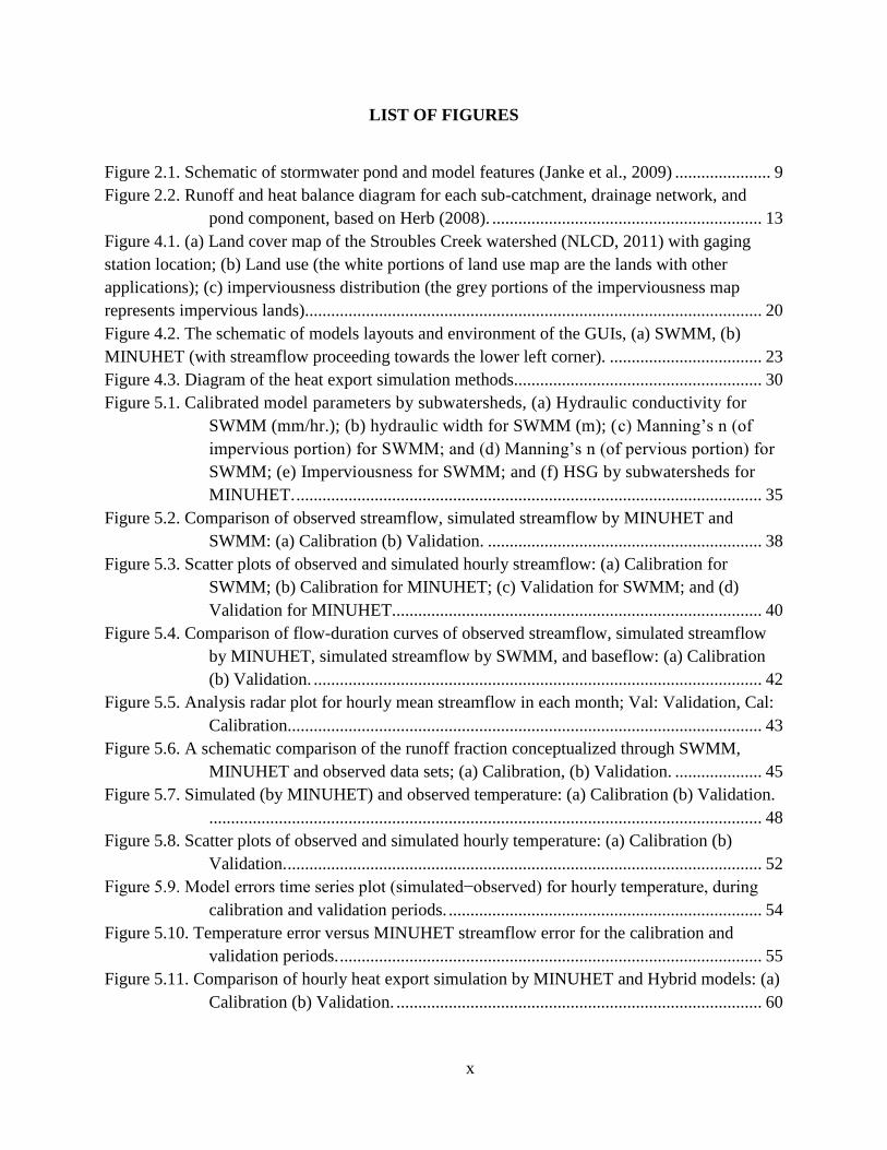
LIST OF FIGURES
Figure 2.1. Schematic of stormwater pond and model features (Janke et al., 2009) ...................... 9
Figure 2.2. Runoff and heat balance diagram for each sub-catchment, drainage network, and
pond component, based on Herb (2008). .............................................................. 13
Figure 4.1. (a) Land cover map of the Stroubles Creek watershed (NLCD, 2011) with gaging
station location; (b) Land use (the white portions of land use map are the lands with other
applications); (c) imperviousness distribution (the grey portions of the imperviousness map
represents impervious lands)......................................................................................................... 20
Figure 4.2. The schematic of models layouts and environment of the GUIs, (a) SWMM, (b)
MINUHET (with streamflow proceeding towards the lower left corner). ................................... 23
Figure 4.3. Diagram of the heat export simulation methods......................................................... 30
Figure 5.1. Calibrated model parameters by subwatersheds, (a) Hydraulic conductivity for
SWMM (mm/hr.); (b) hydraulic width for SWMM (m); (c) Manning’s n (of
impervious portion) for SWMM; and (d) Manning’s n (of pervious portion) for
SWMM; (e) Imperviousness for SWMM; and (f) HSG by subwatersheds for
MINUHET. ........................................................................................................... 35
Figure 5.2. Comparison of observed streamflow, simulated streamflow by MINUHET and
SWMM: (a) Calibration (b) Validation. ............................................................... 38
Figure 5.3. Scatter plots of observed and simulated hourly streamflow: (a) Calibration for
SWMM; (b) Calibration for MINUHET; (c) Validation for SWMM; and (d)
Validation for MINUHET..................................................................................... 40
Figure 5.4. Comparison of flow-duration curves of observed streamflow, simulated streamflow
by MINUHET, simulated streamflow by SWMM, and baseflow: (a) Calibration
(b) Validation. ....................................................................................................... 42
Figure 5.5. Analysis radar plot for hourly mean streamflow in each month; Val: Validation, Cal:
Calibration............................................................................................................. 43
Figure 5.6. A schematic comparison of the runoff fraction conceptualized through SWMM,
MINUHET and observed data sets; (a) Calibration, (b) Validation. .................... 45
Figure 5.7. Simulated (by MINUHET) and observed temperature: (a) Calibration (b) Validation.
............................................................................................................................... 48
Figure 5.8. Scatter plots of observed and simulated hourly temperature: (a) Calibration (b)
Validation. ............................................................................................................. 52
Figure 5.9. Model errors time series plot (simulated−observed) for hourly temperature, during
calibration and validation periods. ........................................................................ 54
Figure 5.10. Temperature error versus MINUHET streamflow error for the calibration and
validation periods. ................................................................................................. 55
Figure 5.11. Comparison of hourly heat export simulation by MINUHET and Hybrid models: (a)
Calibration (b) Validation. .................................................................................... 60
xi
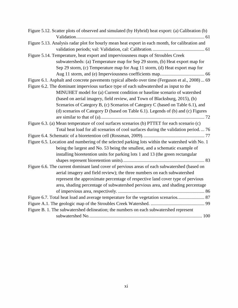
Figure 5.12. Scatter plots of observed and simulated (by Hybrid) heat export: (a) Calibration (b)
Validation. ............................................................................................................. 61
Figure 5.13. Analysis radar plot for hourly mean heat export in each month, for calibration and
validation periods; val: Validation, cal: Calibration. ............................................ 61
Figure 5.14. Temperature, heat export and imperviousness maps of Stroubles Creek
subwatersheds: (a) Temperature map for Sep 29 storm, (b) Heat export map for
Sep 29 storm, (c) Temperature map for Aug 11 storm, (d) Heat export map for
Aug 11 storm, and (e) Imperviousness coefficients map. ..................................... 66
Figure 6.1. Asphalt and concrete pavements typical albedo over time (Ferguson et al., 2008) ... 69
Figure 6.2. The dominant impervious surface type of each subwatershed as input to the
MINUHET model for (a) Current condition or baseline scenario of watershed
(based on aerial imagery, field review, and Town of Blacksburg, 2015), (b)
Scenarios of Category B, (c) Scenarios of Category C (based on Table 6.1), and
(d) scenarios of Category D (based on Table 6.1). Legends of (b) and (c) Figures
are similar to that of (a). ........................................................................................ 72
Figure 6.3. (a) Mean temperature of cool surfaces scenarios (b) PTTET for each scenario (c)
Total heat load for all scenarios of cool surfaces during the validation period. ... 76
Figure 6.4. Schematic of a bioretention cell (Rossman, 2009). .................................................... 77
Figure 6.5. Location and numbering of the selected parking lots within the watershed with No. 1
being the largest and No. 53 being the smallest, and a schematic example of
installing bioretention units for parking lots 1 and 13 (the green rectangular
shapes represent bioretention units). ..................................................................... 83
Figure 6.6. The current dominant land cover of pervious areas of each subwatershed (based on
aerial imagery and field review); the three numbers on each subwatershed
represent the approximate percentage of respective land cover type of pervious
area, shading percentage of subwatershed pervious area, and shading percentage
of impervious area, respectively. .......................................................................... 86
Figure 6.7. Total heat load and average temperature for the vegetation scenarios. ...................... 87
Figure A.1. The geologic map of the Stroubles Creek Watershed. .............................................. 99
Figure B. 1. The subwatershed delineation; the numbers on each subwatershed represent
subwatershed No. ................................................................................................ 100

xii
LIST OF TABLES
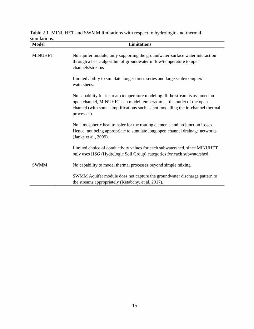
Table 2.1. MINUHET and SWMM limitations with respect to hydrologic and thermal
simulations. ........................................................................................................... 15
Table 4.1. Land use categories of the case study watershed. ........................................................ 19
Table 4.2. Impervious cover of the case study watershed. ........................................................... 19
Table 4.3. Ranges of selected models input parameters based on literature and field data. ......... 25
Table 4.4. Model performance rating system (Moriasi et al., 2007). ........................................... 30
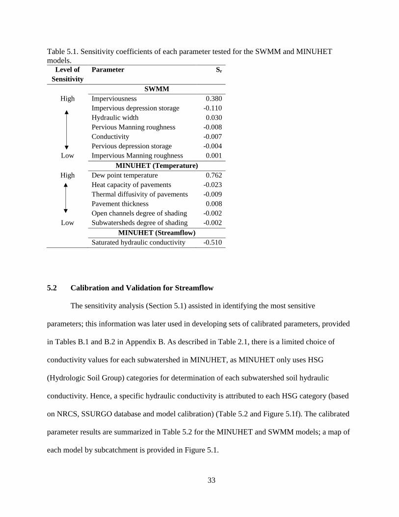
Table 5.1. Sensitivity coefficients of each parameter tested for the SWMM and MINUHET
models. .................................................................................................................. 33
Table 5.2. SWMM and MINUHET hydrologic calibrated input parameters for simulating
streamflow............................................................................................................. 34
Table 5.3. Goodness-of-fit test results for assessing the reliability of calibration and validation
results of SWMM and MINUHET models for streamflow. ................................. 34
Table 5.4. Observed runoff fraction and predicted runoff fraction by SWMM and MINUHET, for
10 storm events, during the calibration and validation periods. ........................... 44
Table 5.5. Goodness-of-fit test results for assessing the reliability of calibration and validation
results of MINUHET model for temperature, mean temperature of simulation and
observation for periods, and percent differences of simulation. ........................... 46
Table 5.6. Quantile estimation of simulated hourly stream temperature compared to measured
stream temperature, for calibration and validation periods. ................................. 57
Table 5.7. Goodness-of-fit test results for assessing the reliability of simulated heat export by
Hybrid and MINUHET models and total heat export calculations throughout the
calibration and validation periods. ........................................................................ 58
Table 5.8. Hydrologic and thermal characteristics of the selected storms for the validation period.
............................................................................................................................... 65
Table 6.1. The properties of pavements and roofs, which are used as input to the MINUHET
model, based on 10 scenarios. ............................................................................... 73
Table 6.2. Heat load and temperature values of cool roof and pavement installation scenarios, at
the outlet of the watershed, during the validation period. ..................................... 75
Table 6.3. Specifications of bioretention cells/infiltration ponds used in SWMM and MINUHET
models to mitigate hydrologic and thermal loads to the Stroubles Creek
watershed. ............................................................................................................. 82
Table 6.4. Hydrologic and thermal results of installation of bioretention systems. ..................... 83
Table 6.5. Various scenarios of using vegetation to reduce thermal effects in the watershed. .... 85
Table 6.6. Heat load and temperature values of canopies scenarios. ............................................ 87
Table B.1. The input watershed parameters for the calibrated SWMM model. ......................... 101
Table B.2. The input watershed parameters for the calibrated MINUHET model. .................... 102
Table C.1. Areas of parking lots and bioretention systems, and number of bioretention units for
each parking lots. ................................................................................................ 104

1
Chapter 1.0 Introduction
Urban development significantly impacts thermal processes within watersheds primarily
through the construction of impervious surfaces for buildings and pavement. These surfaces are
typically darker than natural surfaces, and absorb, and hold more thermal energy, thereby raising
the temperature of runoff. Higher temperature runoff directly impacts receiving streams. Stream
temperature is an important aspect of water quality, playing a critical role in physical, chemical,
and biological processes (Caissie, 2006). Water temperature regimes in streams and rivers are
influenced by changes in air and groundwater temperatures, shading, and alterations to the
hydrologic regime. These changes occur due to stream and land surface modifications, and can
be the result of natural and human-induced activities. The principal anthropogenic and natural
influences on stream temperature regime are described in Table 1.1. The natural processes
affecting stream temperature are solar energy, type of substrate through which the water flows
(Johnson, 2004), heat exchanges across the water surface and streambed (Webb and Zhang,
1999) and the water surface and air, and heat advection from tributaries and groundwater flows
(Evans et al., 1998).
1.1 Criteria on temperature threshold for trout habitat
The recent rapid increase in the thermal pollution of streams due to urbanization and
runoff inputs (which create both intermittent temperature spikes as well as elevating the average
water temperature) has prompted the evaluation of thermal effects on aquatic health and the
associated monitoring studies (Herb et al., 2009a). The sensitivity of trout to daily average and
daily maximum stream temperatures was evaluated (Wehrly et al., 2007). According to the study
findings, the threshold maximum daily temperature varies from 27.5°C for a single-day exposure
to 25.5°C for a seven-day exposure; Single day maximum temperatures (27.5°C) can be used as

2
an acute toxicity threshold for trout. Another study indicated that even at very short exposure
times (10 min), water at 30°C could be fatal for trout (Elliott and Elliott, 1995). Most trout begin
to experience some level of stress at approximately 21°C (Herb et al., 2009a). While many trout
species can withstand gradual warming with changes in seasons, rapid changes in temperature
can be fatal (Agersborg, 1930); hence, high magnitude temperatures and heat loads spikes should
be evaluated.
Table 1.1. The principal anthropogenic and natural influences on stream temperature regime.
Influences Description References
Anthropogenic
Reduced stream shading
and riparian vegetation
Increases net radiation, which results in
stream temperature rise during summer
days up to 10°C.
(Cooter and Cooter,
1990; Hester and
Doyle, 2011)
Reduced groundwater
exchange
Increased groundwater temperature during
baseflow conditions leads to greater
stream temperature.
(Taylor and Stefan,
2009)
Increase in impervious
surface areas
Warmer surface runoff and consequently
warmer streams/rivers immediately after
storms during hot summers.
(Hester and Bauman,
2013; Li et al., 2013)
Heat energy of incoming
wastewater effluents of
industries
Stream temperature increases due to direct
heat inflow to the stream/river.
(Hester and Doyle,
2011)
Channelization Leads to less shading and increases daily
and seasonal temperature fluctuations.
(Hester and Doyle,
2011)
Natural
Type of Substrate Bedrock substrate cools the stream
temperature and dampens diurnal
temperature fluctuations.
(Johnson, 2004)
Heat advection Due to tributaries, and groundwater flows;
can have either cooling effect
(groundwater flows in summer) or
warming effect (groundwater flows in
winter or thermally enriched tributaries).
(Evans et al., 1998)
3
1.2 Research problem and purpose
It is clear that thermally enriched runoff can be harmful to aquatic life; however, only
limited research and guidance is available for predicting these impacts at the watershed level. In
Blacksburg, Virginia, Stroubles Creek is a stream with a watershed is highly urbanized,
particularly in its headwaters, due to the presence of downtown Blacksburg, Virginia and a
portion of the campus of Virginia Tech. These urbanized areas impact Stroubles Creek
significantly via thermal loads from urban runoff. While several studies (Hester and Bauman,
2013; Long and Dymond, 2014) have investigated thermal loads in Stroubles, none has been
conducted at the watershed scale or analyzed mitigation measures. Addressing these impacts on a
watershed basis is needed. Stroubles Creek provides an excellent case study site due to extensive
monitoring and available geodatabase information, relatively small size, and extensive
impervious coverage in headwater regions. Thus, the purpose of this research is to evaluate the
thermal processes occurring within the Stroubles Creek watershed and their impacts to
downstream aquatic health.

4
Chapter 2.0 Literature Review
2.1 Human effects on stream thermal processes
Water temperature regimes in streams and rivers are influenced by changes in air and
groundwater temperatures and alterations to the hydrologic regime. In addition, land surface
temperatures have substantial effects on stream/river temperature. These changes occur because
of natural and human-modified energy exchange processes. The sections below discuss the major
anthropogenic influences on stream/river temperature.
Altering stream shading by removing vegetation increases net radiation, resulting in
daytime stream temperature increases of up to 7°C (Cooter and Cooter, 1990) and 10°C (Hester
and Doyle, 2011). This impact is more critical in summer, due to greater solar radiation (Jones
and Hunt, 2009).
Groundwater flow is another significant factor in the temperature of gaining streams,
especially during periods with low precipitation. On the other hand, if a stream is losing, then
stream temperature is unaffected by groundwater temperature. Groundwater flow and
temperature are influenced by climate, hydrogeology, and surface water temperature (Taylor and
Stefan, 2009). Taylor and Stefan (2009) investigated the effects of land use and climate change
on shallow groundwater temperature in Minneapolis-St. Paul, MN. Their analysis showed that
pavement is the main controlling factor of groundwater temperature, as documented by a 3°C
increase in groundwater temperatures under paved areas, as compared to temperatures in
unpaved areas. According to their study, urbanization, which leads to less pervious lands and
infiltration, increases groundwater temperature, which leads to increased stream temperatures
during baseflow conditions. When urbanization and climate change influences are considered
together, groundwater temperature was projected to rise by 5°C, and that during the summer,

5
groundwater influence on stream temperature is generally greater than climate change influence.
Conversely, in another study conducted by Herb et al. (2009a), stream temperature was highly
correlated with air temperature, possibly due to low groundwater inputs. As a result of the low
groundwater inputs, the stream may be particularly sensitive to climate change.
During warm season storm events, thermal energy, which is absorbed by impervious
surfaces and pavements, is conveyed by surface runoff to streams, leading to warmer surface
runoff and thus warmer streams and rivers. Thompson et al. (2005) conducted a study on thermal
pollution differences between asphalt pavement and turfgrass surfaces under a range of simulated
rainfall conditions, using experimental plots. According to their findings, solar radiation was the
most important factor affecting asphalt surface runoff temperature. Before the storm event
simulations, the asphalt and sod average surface temperatures were 43.6°C and 23.3°C,
respectively. Immediately after simulated rainfall events, the pavement and turfgrass surface
temperatures declined an average of 12.3°C and 1.3°C, respectively. Increasing turf areas within
the watershed was shown to be highly effective in mitigating urban runoff temperature and heat
energy (Thompson et al., 2008). In a similar study, the effect of permeable and impermeable
pavements on surface temperature reduction and cooling of surface runoff temperature was
investigated (Li et al. 2013). The authors assessed three kinds of permeable pavements including
interlocking concrete paver, asphalt concrete, and Portland cement concrete, and found that
permeable pavement reduced surface temperature and thence runoff temperature; conversely,
impervious surfaces led to warmer surface runoff and consequently higher stream temperature.
Overall, higher impervious surfaces in urban areas resulted in increased average and peak runoff
temperature and variability (Li et al., 2013). Immediately after a summer storm event, stream
temperature increases dramatically mainly due to two reasons; 1) warmer surface runoff due to

6
more developed areas (Li et al., 2013); and 2) less groundwater discharge to the stream due to
less infiltration in watersheds (Taylor and Stefan, 2009). Groundwater aquifers play a dampening
role, and decrease stream temperature during warm months of the year (Herb, 2008).
Temperature surges in runoff: Temperature surges in runoff are a common phenomenon
in urban areas during hot summers, resulting in spikes in receiving stream temperature, health
impacts to aquatic biota through rapid changes of temperature, and increased pollutant loading
(Hester and Bauman, 2013). Hester and Bauman (2013) monitored urban storm sewer outfalls in
Blacksburg, Virginia and assessed runoff temperatures. Temperature surges occurred
approximately a dozen times per summer months (during early June to mid-August) ranging up
to 8.1°C with average duration of 2 hr. in a stream and up to 11.2°C with average duration of 7
hr. in a detention pond. Surges were more common in the afternoon, but were observed during
all times of the day (Hester and Bauman 2013).
Temperature changes due to industrial wastewater effluents, dam releases, and water
diversions: Wastewater discharges entering streams are considered continuous sources.
Wastewater increases stream temperature over time, mainly because of heat inflow to the
stream/river. Increased stream temperature by aforementioned influence (wastewater discharge)
is more prominent during the winter seasons, when there is a large gap between stream
temperatures and effluent temperatures levels (Xin and Kinouchi, 2013). Releases from
reservoirs increases the stream/river temperature during winter, mainly due to water releases
from the lower layers of a thermally stratified reservoir. These influences are most prominent in
headwater streams. Some anthropogenic influences have cooling effects on stream temperature,
such as diverting tributaries (Hester and Doyle, 2011). Xin and Kinouchi (2013) found that the
Tama River, a major river system running through central Tokyo had significantly greater water

7
temperatures in winter due to warm effluent discharges from wastewater treatment facilities. A
large water temperature increase was observed due to the effects of water withdrawals, in
summer (Xin and Kinouchi, 2013). Results indicated that the largest contributions to water and
heat gains were attributable to wastewater effluents, while other factors such as groundwater
recharge acted as heat energy sinks, specifically in summer. Heat exchange at the air–water
interface contributed less to heat budgets in winter and summer seasons for all river segments.
Therefore, the effect of heat exchange through the air–water interface was minor (Kinouchi et
al., 2007; Xin and Kinouchi, 2013).
Channelization: Stream channelization causes streamflow to move more quickly, and
leads to less shading (mainly because of reduced stream-bank vegetation). Channelization is
most prominent is urban areas and increases daily and seasonal temperature fluctuations (Gorney
et al., 2012)
2.2 Stormwater control measures to mitigate thermal pollution
One tool for mitigating thermal pollution is infiltrative stormwater control measures
(SCMs), also known as urban stormwater best management practices (BMPs). The purpose of
BMPs is to mimic predevelopment hydrology, water quality, and temperature of runoff.
Infiltrative BMPs may be the most effective technique to mitigate thermal impacts of runoff on
the environment. Infiltration recharges the groundwater and becomes part of the baseflow to
coldwater streams. In addition to single infiltrative BMP types, infiltrative BMPs in series (such
as infiltration ponds and bioretention systems), known as an “infiltrative BMP treatment trains”,
provide thermal treatment of runoff.

8
Restoration of the aquatic habitat in urban streams should consider potential strategies to
mitigate thermal pollution from impervious surfaces. Once such BMP is bioretention, which has
been shown to be effective in reducing maximum and median runoff temperatures (Jones and
Hunt, 2009). However, several studies (Dietz and Clausen, 2005; Hester and Bauman, 2013;
Jones and Hunt, 2009; Long and Dymond, 2014) have suggested that these practices alone will
likely be insufficient to maintain runoff temperatures from an urban watershed during the
summer below the toxicity threshold for trout (21°C).
Jones and Hunt (2010) investigated the effects of wetlands and wet ponds on the urban
runoff temperature in western North Carolina for acute toxicity to trout populations. The paved
surfaces during summer months absorb and retain the solar radiation, which transfer this thermal
energy to urban runoff during rainfall events. The authors found that the volume of enriched
runoff could have harmful effects on aquatic systems. Jones and Hunt (2010) found that the
parking lot runoff temperatures were far higher than 21°C, which is a threshold for trout. The
wetlands and wet ponds raised temperatures between their respective inlets and outlets,
indicating these BMPs were a source of thermal pollution, although the wetland outflow
temperatures increase in temperature was less than what was observed in the wet pond, mainly
due to the effect of wetlands shading vegetation. The authors found that underground pipes that
conveyed runoff from the wetland to the receiving stream were effective in cooling discharges
(Jones and Hunt, 2010). According to Jones et al. (2012) findings, BMP practices alone cannot
be effective separately (or even as a train) in reducing thermal pollution of urban runoff. In other
words, with the threshold for acute toxicity for trout being 21°C, current practices were unable to
mitigate temperatures to below this level during the summer. Hence, Jones et al. (2012) suggest
that other factors related to catchments characteristics and a watershed-scale plan or response can

9
be used to mitigate thermal pollution. These actions include tree canopies for increased shading
of streams to reduce median and maximum surface temperature of the contributing catchment,
and light-colored chip seal application to reduce runoff temperatures, in addition to
implementation of infiltrative practices such as bioretention. These factors reduce the median
and maximum surface runoff of parking lot. Utilizing BMP trains together with in-catchment
control factors of stormwater may lead to better mitigation of thermal pollution.
Janke et al. (2009) developed an unsteady, 1-D model to simulate heat transfer within a
detention pond to assess thermal pollution of a cold-water stream in Minnesota. The authors
simulated the system for six years using observed rainfall events and found the long-term
average outflow temperature was 1.2°C higher than the inflow temperature. However,
temperature spikes in the stream were reduced mainly due to the reductions in the peak runoff
rate. The schematic of stormwater pond and model features is shown in Figure 2.1 (Janke et al.,
2009).
Figure 2.1. Schematic of stormwater pond and model features (Janke et al., 2009)

10
Jones and Hunt (2009) investigated the effect of bioretention on runoff temperature. The
smaller bioretention cells reduced peak and median discharge water temperature significantly. In
comparison, the proportionally larger bioretention cell was unable to match the lower
temperature of the smaller bioretention cell due to a much larger runoff volume input. This study
points out that while small and large bioretention cells provided temperature mitigation and
thermal load reduction, outflow temperatures still exceeded 21°C. The authors suggest it will be
necessary to implement more bioretention cells, to achieve a healthy stream in a trout habitat. A
key finding of Jones and Hunt (2009) study was that deeper bioretention cells lead to cooler
runoff temperatures during the summer months.
Dietz and Clausen, (2005) investigated the temperature mitigation of roof runoff by roof
gardens in all seasons of a year; while there was no installed control roof to evaluate the
effectiveness of roof gardens compared to a baseline scenario. The ANOVA statistical test
results on the difference between roof runoff temperature (produced by asphalt shingle roofs)
and roof gardens underdrain-systems outflow temperature showed no significant differences
between the inflow and outflow temperature among all seasons. Another study in Blacksburg,
southwest Virginia by Long and Dymond (2014) was conducted through 10 artificial runoff
events generated by a nearby fire hydrant. Runoff median and maximum temperature were
reduced by 8.8°C and 8.6°C, respectively, between the inlet and discharge of the bioretention
cell. The bioretention reduced runoff volume by 1.4 m3, or 10%, and reduced heat export from
the site by 37 MJ/m3. Bioretention systems, in comparison to wetlands and wet ponds, increases
runoff reduction, and results in less heat export (Jones and Hunt, 2009; Jones et al., 2012; Long
and Dymond, 2014). Bioretention systems are particularly effective at runoff and thermal load

11
reduction when installed in coarse textured soils, such as well sorted gravel, well sorted sand or
sand and gravel, which have greater hydraulic conductivity (Long and Dymond, 2014).
2.3 Review of models and empirical equations to simulate water temperature
Numerous process-based models and empirical relationships have been developed for
simulating runoff quantity and temperature from urban surfaces during rainfall events. For
example, a hydro-thermal model was developed to simulate runoff temperatures from a paved
surface (Janke et al., 2009). The authors found that heat export was strongly correlated with the
rainfall parameters such as intensity, duration, and temperature; higher intensities resulted in
lower runoff temperature. The authors found that any activities that alter the timing or magnitude
of streamflow regime likely would alter stream temperature (Janke et al., 2009). A physically
based model was assessed to estimate the spatiotemporal variability of river water temperature in
summer at a regional scale (Beaufort et al., 2016). Air temperature was used as an index to
predict stream temperature (Morrill et al., 2005), using a nonlinear regression equation (Eq. 1).
𝑇𝑠 = 𝜇 +(𝛼−𝜇)
1+𝑒(𝛾∗(𝛽−𝑇𝑎)) Eq. 1
Where Ts= estimated stream temperature (°C); Ta = is measured air temperature for the period of
interest (°C); µ=minimum stream temperature (°C); α=maximum stream temperature (°C); and
β= inflection point, defined as the function of the steepest slope of the Ts function.
Brogan (2003) used Equilibrium Temperature (Eq.T), which is the stream temperature at
which the sum of all heat fluxes through the stream is 0.0, as an indicator of stream temperature
(ST). The relationship between Eq.T and ST was assessed using an empirical linear regression
relationship (Bogan, 2003).
12
Arrington et al. (2004) developed and applied the Thermal Urban Runoff Model (TURM)
to evaluate the impact of urbanized watersheds on stream temperature. TURM predicts surface
runoff and runoff temperature from pervious and impervious surfaces. The TURM model uses
the curve number method (NRCS, 1986) for simulating runoff, so it is applicable mainly for
design storm events.
SNTEMP (Stream Network Temperature Model), a 1-D steady-state heat transport
model, simulates daily average and maximum stream temperatures versus downstream distance
as function of groundwater inputs, channel geometry, discharge, climate, and riparian shading
(Herb et al., 2009a). Current stream temperature models are reach-based models working at
daily/hourly time steps. Simple empirical models are inadequate or inappropriate for catchment-
scale applications, while spatially distributed physical models require substantial field-measured
input data to run.
The Minnesota Urban Heat Export Tool (MINUHET) was developed to address some of
the shortcomings of models described above. MINUHET is both an event-based and continuous
simulation model that produces a time series of runoff temperature and heat loading at the
catchment outlet. MINUHET includes three main simulation modules for hydrologic routing,
hydrologic/thermal modeling of watersheds, and hydrologic and thermal effects of SCMs.
Runoff is assumed to be thin (sheet flow) and well mixed, with the heat capacity of pure water.
MINUHET enables the user to simulate landuse effects on overland runoff temperature and heat
loading to a stream, thereby predicting the thermal impact of landuse on receiving streams (Janke
et al., 2013). In its current implementation, MINUHET includes all major hydrologic modules
and heat transfer processes applicable to a small urban watershed. A schematic diagram showing
the balance of runoff and heat flux for each sub-catchment, drainage network, and pond
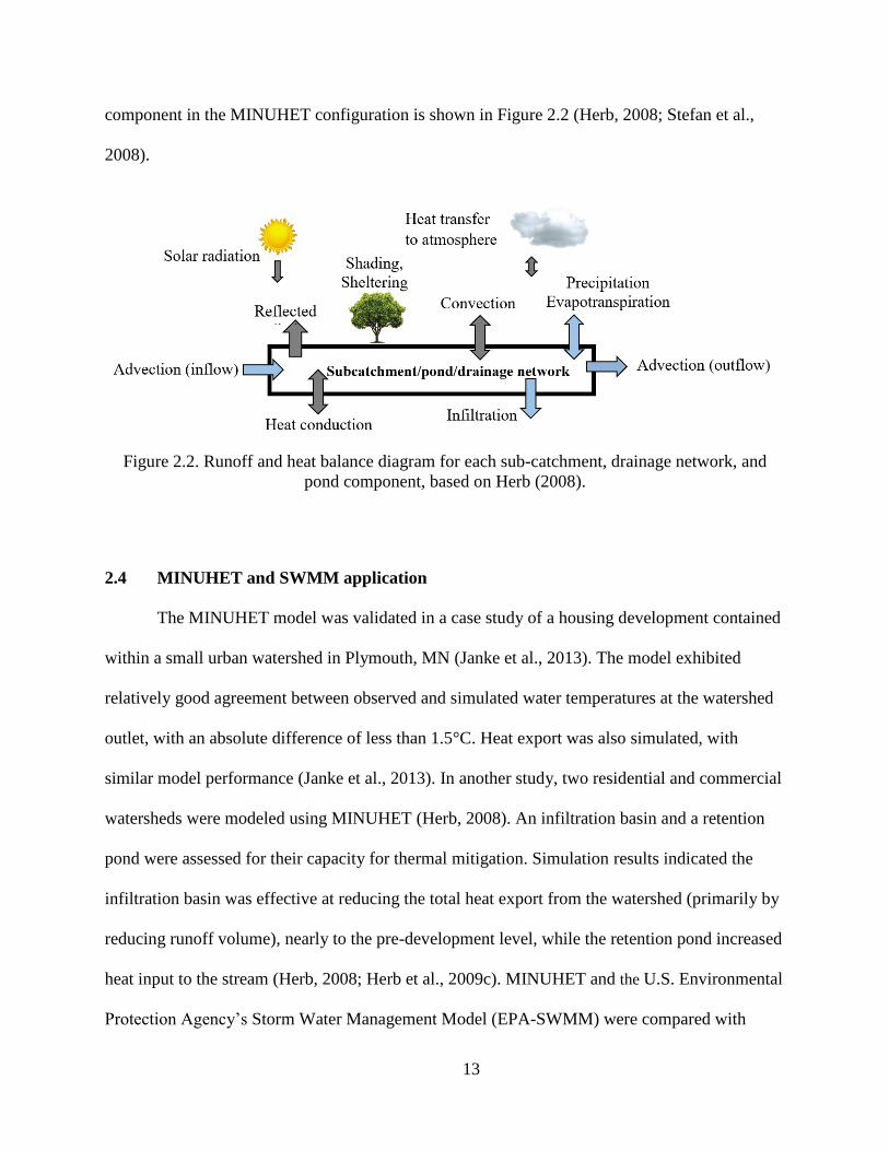
13
component in the MINUHET configuration is shown in Figure 2.2 (Herb, 2008; Stefan et al.,
2008).
Figure 2.2. Runoff and heat balance diagram for each sub-catchment, drainage network, and
pond component, based on Herb (2008).
2.4 MINUHET and SWMM application
The MINUHET model was validated in a case study of a housing development contained
within a small urban watershed in Plymouth, MN (Janke et al., 2013). The model exhibited
relatively good agreement between observed and simulated water temperatures at the watershed
outlet, with an absolute difference of less than 1.5°C. Heat export was also simulated, with
similar model performance (Janke et al., 2013). In another study, two residential and commercial
watersheds were modeled using MINUHET (Herb, 2008). An infiltration basin and a retention
pond were assessed for their capacity for thermal mitigation. Simulation results indicated the
infiltration basin was effective at reducing the total heat export from the watershed (primarily by
reducing runoff volume), nearly to the pre-development level, while the retention pond increased
heat input to the stream (Herb, 2008; Herb et al., 2009c). MINUHET and the U.S. Environmental
Protection Agency’s Storm Water Management Model (EPA-SWMM) were compared with
14
respect to runoff generation during a single rainfall event. Both models had similar results for
runoff volume (Herb, 2008).
Several public domain hydrologic models are capable of simulating runoff in urban
watersheds, e.g., the Hydrologic Modeling Systems, or HMS, Hydrologic Simulation Program-
Fortran, or HSPF and SWMM. SWMM is a dynamic hydrology-hydraulic model, which is
employed to simulate stormwater quantity and quality for event-based and continuous-based
scenarios. The current SWMM configuration determines runoff by evaluating infiltration
processes using the Green-Ampt equation (Green and Ampt, 1911), Horton, or Curve Number
methods and then makes use of the dynamic wave, kinematic wave, or steady-flow
approximations for runoff routing. The capabilities of these models for simulating runoff
processes exceed that of MINUHET; the strength of MINUHET is its unique ability to simulate
heat export and runoff temperature, thus providing a tool for evaluating the thermal impacts of
urban runoff on receiving water bodies.
The limitations of MINUHET and SWMM are shown in Table 2.1. Unlike SWMM,
MINUHET does not include a comprehensive aquifer module; however, SWMM does not have
the capability to model thermal processes (Table 2.1). While individual MINUHET components
have been validated, (Herb, 2008; Janke et al., 2013), to date, MINUHET has not been applied to
a larger urbanized watershed which includes open channels, detention/retention ponds, and a
variety of urban land covers (Janke et al., 2013).
15
Table 2.1. MINUHET and SWMM limitations with respect to hydrologic and thermal
simulations. Model Limitations
MINUHET No aquifer module; only supporting the groundwater-surface water interaction
through a basic algorithm of groundwater inflow/temperature to open
channels/streams
Limited ability to simulate longer times series and large scale/complex
watersheds.
No capability for instream temperature modeling. If the stream is assumed an
open channel, MINUHET can model temperature at the outlet of the open
channel (with some simplifications such as not modelling the in-channel thermal
processes).
No atmospheric heat transfer for the routing elements and no junction losses.
Hence, not being appropriate to simulate long open channel drainage networks
(Janke et al., 2009).
Limited choice of conductivity values for each subwatershed, since MINUHET
only uses HSG (Hydrologic Soil Group) categories for each subwatershed.
SWMM No capability to model thermal processes beyond simple mixing.
SWMM Aquifer module does not capture the groundwater discharge pattern to
the streams appropriately (Ketabchy, et al. 2017).

16
Chapter 3.0 Research Objectives
Despite the significance of thermal issues associated with urban runoff, only a few tools
exist that are capable of simulating runoff temperature and heat loads. The best available tool,
MINUHET, has a limited ability to simulate complex urban watersheds; such analyses are often
performed using SWMM. The current SWMM configuration has no capability to model thermal
processes. The objective of this research is to apply MINUHET and SWMM to a medium-sized
urban watershed, Stroubles Creek, in Blacksburg, Virginia. Stroubles Creek has several
monitoring locations at which streamflow, groundwater level, climatological data, and water
temperatures have been recorded for several years at the Virginia Tech Stream Research,
Education, and Management Lab (StREAM Lab)
(https://www.bse.vt.edu/research/facilities/StREAM_Lab.html). The StREAM Lab is a
nationally recognized research facility that monitors streamflow quantity and quality data.
MINUHET and SWMM models were developed, calibrated, and validated using data from two
StREAM Lab monitoring stations. Model sensitivity was assessed and event-based and
continuous streamflow estimates by models were compared. Then SWMM-simulated streamflow
and water temperature from MINUHET were combined in a unique, hybrid approach to simulate
heat export from the watershed (Hybrid model). In the next step, the comparison of MINUHET
and Hybrid models capabilities for simulating heat export was conducted. Lastly, the effects of
retrofitting the watershed for thermal mitigation using infiltration practices and increased canopy
shading were evaluated. While these practices have a demonstrated ability to mitigate
downstream water temperatures, this effect has not been assessed at the watershed scale. The
primary purpose of the assessment is to provide guidance in achieving temperature regimes that
meet aquatic health criteria for sensitive species such as trout. This standard is likely going to be

17
difficult to achieve. To address this issue, a more general approach was developed to assess the
relationship between downstream heat loads as a function of upstream infiltration capacity, and
thermal mitigation practices such as cool pavement installations.

18
Chapter 4.0 Materials and Methods
4.1 Site Description of the Case Study
The 58-km2 Stroubles Creek watershed is located in Montgomery County, Virginia and is
tributary to the New River, part of the Ohio-Mississippi River-Gulf of Mexico system. The study
was conducted on a 14.1-km2 upstream portion of the Stroubles Creek watershed (Figure 4.1a).
A monitoring station operated by the Virginia Tech StREAM Lab is located at the
watershed outlet as is shown on Figure 4.1a. Land cover is primarily urbanized (75%), with 21%
agricultural and 4% forest, based on the 2011 National Land Cover Database (Figure 4.1a). The
Duck Pond (Figure 4.1a) acts as a divider between the highly urbanized headwater portion
(approximately 7.8 km2 in area) and the downstream agricultural and forested portion of the
Stroubles Creek watershed, the entirety of which is referred to as the Main watershed. The
Central Branch and the Webb Branch are the two tributaries that merge at the Virginia Tech
Duck Pond to form Stroubles Creek (Figure 4.1a).
Many forms of channel modification exist throughout the watershed, including piped
stream reaches, ponds, and channelization. The Town of Blacksburg land use classifications
(http://www.gis.lib.vt.edu/gis_data/Blacksburg/GISPage.html) and geographic information
system (GIS) data were used for the watershed (Table 4.1 and Figure 4.1b). The breakdown of
imperviousness across the watershed and imperviousness distribution, computed by tracing aerial
photography (http://www.gis.lib.vt.edu/gis_data/Blacksburg/GISPage.html) are shown in Table
4.2 and Figure 4.1c, respectively. Imperviousness of the entire watershed is 32%, with buildings
and parking lots constituting approximately 61% of the total impervious area (Table 4.2).

19
Characterized by limestone and dolomite formations, the Stroubles Creek streambed is
formed of gravel and cobbles and has alluvium-floodplain deposits of stratified clay, sand, and
silt (Mostaghimi et al., 2003). The dominant Hydrologic Soil Group of the upstream of
watershed is category C (NRCS, 2007), while downstream of Duck Pond consists mainly of
category B, or silt loam and loam (Refer to Appendix A for the Stroubles Creek geologic map
and respective description). The depth to the water table in the downstream portion of the
watershed is approximately 1 m and mean annual precipitation is approximately 1030 mm
(Hofmeister et al., 2015).
Table 4.1. Land use categories of the case study watershed.
Land use type Percentage
Commercial/Industrial 4.0
Very low density residential and agricultural 12.8
Low density residential 17.1
Medium density residential 4.0
High density residential 7.0
University 25.4
Park land/Opens spaces 3.3
Civic 5.5
Others 20.9
Table 4.2. Impervious cover of the case study watershed.
Impervious land cover type % of Impervious areas
Building 28.4
Sidewalks 10.3
Ponds 1.8
Streets 22.4
Parking lots 31.3
Driveways 4.1
Others 1.7
Percent imperviousness of
StREAM Lab watershed 32.0

20
Figure 4.1. (a) Land cover map of the Stroubles Creek watershed (NLCD, 2011) with gaging
station location; (b) Land use (the white portions of land use map are the lands with other
applications); (c) imperviousness distribution (the grey portions of the imperviousness map
represents impervious lands).
21
4.2 Data Collection
The Town of Blacksburg and Virginia Tech provided storm sewer and surface elevation
GIS data. Soil information was acquired from the Soil Survey Geographic Database (SSURGO)
of Natural Resources Conservation Service (NRCS)
(https://websoilsurvey.sc.egov.usda.gov/App/HomePage.htm), at the watershed scale. At the
StREAM Lab monitoring station, a pressure transducer (CS451, Campbell Scientific Inc., Logan,
UT, U.S.A., water level resolution: 0.0035% FS) and a datalogger (CR1000, Campbell Scientific
Inc., U.S) record stream stage every 15 minutes (Figure 4.1a). Stage is converted to discharge
using a rating curve, which was developed based on Stroubles Creek stage-discharge historical
data. In addition, an YSI Sonde (6920 V2, Xylem Analytics, U.S, +/- 0.15°C) records water
temperature. Temperature measurements are checked against a calibrated thermometer to
calibrate the Sonde. Precipitation is recorded by Town of Blacksburg and the meteorology
station of the StREAM Lab, on 15 minutes time steps. A tipping bucket rainfall sensor (TR-
525USW, Texas Electronics, Inc., Dallas, TX, +/- 1%) is to monitor precipitation at the Town of
Blacksburg weather station. Solar radiation, wind speed, relative humidity, and air temperature
are measured in every 30 minutes at the StREAM Lab weather station, located approximately
300 m downstream of the Stroubles Creek monitoring station (Figure 4.1a). StREAM Lab sensor
specifications are as follows: (1) rain, TE525, Campbell Scientific, U.S, 1.0% up to 2 in/hr.; (2)
wind speed, 034A/034B, Campbell Scientific, U.S, 0.1 m/s; (3) air temperature and relative
humidity, CS215, Campbell Scientific, U.S, ±2% at 25°C); and (4), solar radiation, CS300,
Campbell Scientific, U.S, ±5% for daily total radiation. A datalogger (CR1000, Campbell
Scientific Inc., U.S), and a radio modem as the communication equipment (Digi X-Tend 1 W
900mHz spread spectrum, Digi International Inc., MN) are used to store and transmit the weather
22
station data at StREAM Lab. Cloud cover data every 20 minutes were acquired through NOAA
(https://www.ncdc.noaa.gov/cdo-web/). The depth to groundwater is measured every 10 minutes
in two piezometers installed in the floodplain adjacent to weather station using two similar water
level loggers (CS451, Campbell Scientific, U.S, water-level resolution: 0.0035% FS). The data-
sampling period was split into two warm periods of mid-June to late September, for 2015 and
2016. The 2015 warm period was drier and relatively cooler than the 2016 warm period. The
total rainfall and average hourly temperature during the two measurement periods were 20.6 cm
and 20.1 +/-5°C and 34.5 cm and 21.0 +/- 4.6°C for 2015 and 2016, respectively. The mean
discharge for Stroubles Creek during the 2015 and 2016 warm periods was 0.15 and 0.24 m3s-1,
respectively. Groundwater is assumed to be the main control of discharge (Hofmeister et al.,
2015); hence, due to minimal precipitation, the stream was at baseflow during much of the two
monitoring periods.
4.3 SWMM and MINUHET Models Setup
A total of 43 subwatersheds and 30 detention/retention ponds were delineated within the
watershed. The urbanized portion of the watershed (upstream of the Duck Pond) is more
complex than the watershed downstream of the Duck Pond due to presence of intensive urban
development. Hence, the subwatershed delineation was conducted manually in the urbanized
portion of the watershed based on the locations of the ponds and the stormwater drainage
network/infrastructure. Downstream of the Duck Pond, elevation data were used to delineate the
subwatersheds using a GIS application (the watershed extension) (Ketabchy et al., 2016a).
Stroubles Creek was modeled as a pervious open-channel system with irregular cross-sections in
downstream and impervious rectangular cross-sections beneath the Virginia Tech campus, for
both the MINUHET and SWMM configurations. The outlet of each pond was modeled as a weir

23
structure. Routing computations were conducted for each pond, and the stage-storage
(bathymetry) characteristics of ponds were computed through Town of Blacksburg information
and the watershed data elevation models (DEMs). The lengths of the impervious and pervious
areas of each subwatershed were estimated from the longest overland runoff paths, while these
runoff paths were used to calculate the hydraulic width of each subcatchment, a required SWMM
parameter of each subcatchment. Green-Ampt infiltration and dynamic wave methods were used
for the infiltration and routing models of SWMM, respectively. Groundwater table elevation was
quantified using geological maps of Geology and Mineral Resources Division of Commonwealth
of Virginia (Appendix A) (https://www.dmme.virginia.gov/dgmr/mapspubs.shtml), and data
from the StREAM Lab pre-installed floodplain piezometers. To build the model structure and
conduct the sensitivity analysis, PC-SWMM was used to directly import spatial information and
attributes from a geodatabase GIS. MINUHET was used to simulate the time series of runoff
temperature for the impervious and pervious sections of a subcatchment. Based on these two
simulated time series, the watershed thermal module of MINUHET uses a simple mixing method
to produce composite hydrograph and time series of runoff temperature. The schematic of
SWMM and MINUHET graphic user interfaces (GUIs) and structures are shown in Figure 4.2.
Figure 4.2. The schematic of models layouts and environment of the GUIs, (a) SWMM, (b)
MINUHET (with streamflow proceeding towards the lower left corner).
24
4.4 Sensitivity Analysis
A sensitivity analysis was conducted to assess the influence of individual model input
parameters on model (SWMM and MINUHET) streamflow and temperature output. To perform
the sensitivity analysis and identify the crucial input parameters, the value of a particular input
parameter was varied while holding all other parameters constant during the simulation.
Identification of the most sensitive parameters focuses the calibration on a subset of input
parameters (Ahmadisharaf et al., 2016; Janke et al., 2013; Nayeb Yazdi et al., 2015).
The sensitivity of the following SWMM and MINUHET model outputs were quantified:
average total streamflow and streamflow-averaged temperature, throughout the calibration period
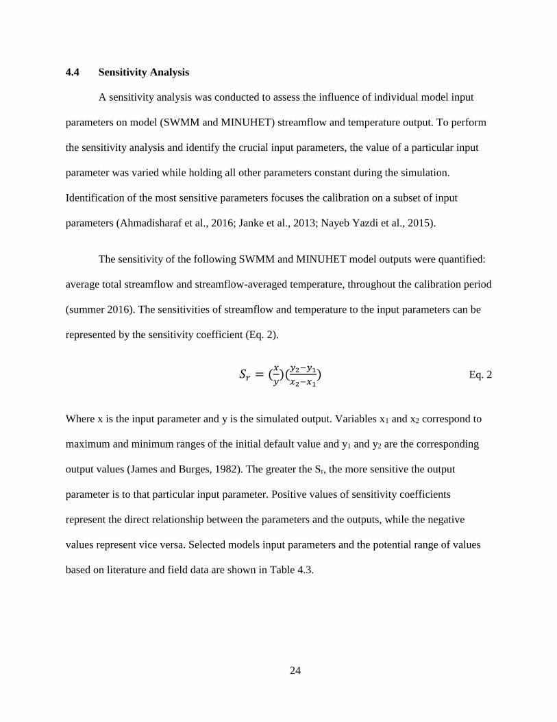
(summer 2016). The sensitivities of streamflow and temperature to the input parameters can be
represented by the sensitivity coefficient (Eq. 2).
𝑆𝑟 = (𝑥
𝑦)(
𝑦2−𝑦1
𝑥2−𝑥1) Eq. 2
Where x is the input parameter and y is the simulated output. Variables x1 and x2 correspond to
maximum and minimum ranges of the initial default value and y1 and y2 are the corresponding
output values (James and Burges, 1982). The greater the Sr, the more sensitive the output
parameter is to that particular input parameter. Positive values of sensitivity coefficients
represent the direct relationship between the parameters and the outputs, while the negative
values represent vice versa. Selected models input parameters and the potential range of values
based on literature and field data are shown in Table 4.3.

25
Table 4.3. Ranges of selected models input parameters based on literature and field data.
Parameter Unit Value Range References
SWMM
Imperviousness % ±15% of each
subwatershed
(Kong et al., 2017)
Hydraulic width (H.W.) m ±10% of each
subwatershed
(James et al., 2010)
Impervious Manning roughness - 0.01–0.03 (Wanielista MP, 1997)
Pervious Manning roughness - 0.02–0.45 (Huber and Dickinson, 1988)
Impervious depression storage mm 0.3–4.0 (Huber and Dickinson, 1988)
Pervious depression storage mm 2.5–7.5 (Huber and Dickinson, 1988)
Conductivity mm/hr. ±20% of initial values U.S Department of
Agriculture
MINUHET
Heat capacity of pavements J/m3.°C 1.9-3.7×10⁶ (Kavianipour and Beck, 1977)
Thermal diffusivity of pavements m2/s 4.42×10⁻⁷-14.4×10⁻⁷ (Luca and Mrawira, 2005)
Pavement thickness m 0.102-0.203 (Kavianipour and Beck, 1977)
Saturated hydraulic conductivity m/s 3.61×10⁻⁷ (HSG: D) -
2.75×10⁻⁵ (HSG: A)
(Rawls, 2006)
Subwatersheds degree of shading % ±15% of initial
estimate
Aerial photos and field data
Open channels degree of shading % ±15% of initial
estimate
Aerial photos and field data
Dew point temperature °C ±2°C of initial
calculated values
(Stefan et al., 2008)
4.5 Calibration and Validation at the Watershed Outlet
SWMM and MINUHET inputs were chosen for the models calibration process based
upon the sensitivity analysis, current manuals, field data, model defaults, and literature sources.
Sensitivity analysis indicated the most sensitive parameters, which were adjusted to optimize
agreement between the simulated and observed values. Measured streamflow at StREAM Lab
between June 15 and September 30 of 2016 were selected to represent summer conditions and
were used to calibrate the models; streamflow for the same period in 2015 was used for model
validation. The focus is on the summer periods because this is the critical period for temperature
in terms of sensitive species, such as trout. The goal of model validation was to assess whether

26
the calibrated model was able to mimic streamflow behavior for events outside of the calibration
period.
To build and run the thermal module of MINUHET, the tool requires climate data as an
input, including solar radiation, air temperature, relative humidity, wind speed, cloudiness, and
precipitation. Climate files for the calibration and validation periods were built using 15 minute-
intervals. The MINUHET model was calibrated for thermal processes by adjusting the heat
capacity of pavement, thermal diffusivity of pavement, and pavement thickness to match
observed water temperature.
Goodness of fit criteria: The efficacy of calibration and validation results were evaluated
using a group of goodness-of-fit tests that are described in the following sections.
Nash-Sutcliffe efficiency (NSE): NSE specifies the relative magnitude of the observed
data variance compared to the residual (observed-simulated) variance (Nash and Sutcliffe, 1970).
It represents how well the plot of predicted versus observed data fits a 1:1 line. NSE is calculated
as shown in Eq. 3.
𝑁𝑆𝐸 = 1 − [∑ (𝑌𝑖
𝑜𝑏𝑠−𝑌𝑖𝑠𝑖𝑚)
2𝑛𝑖=1
∑ (𝑌𝑖𝑜𝑏𝑠−𝑌𝑚𝑒𝑎𝑛𝑛
𝑖=1 )2] Eq. 3
Where Yiobs is the ith observation for the observation data set, Yi
sim is the ith predicted value for the
simulated data set, Ymean is the mean of observed data set, and n is the total number of
observations. NSE equal to 1.0 is the optimal value, while NSE ranges between −∞ and 1.0.
Percent bias (PBIAS): PBIAS calculates the average tendency of the simulated data set to
be smaller or larger than the observed data set (Gupta et al., 1999). The optimal value of PBIAS
is 0.0, with lower values representing more accurate model prediction. Negative values represent

27
model over-prediction bias, while positive values represent model under-prediction bias. It is
calculated as shown in Eq. 4.
𝑃𝐵𝐼𝐴𝑆 = [∑ (𝑌𝑖
𝑜𝑏𝑠−𝑌𝑖𝑠𝑖𝑚)∗100𝑛
𝑖=1
∑ (𝑌𝑖𝑜𝑏𝑠)𝑛
𝑖=1
] Eq. 4
RMSE-observations standard deviation ratio (RSR): RMSE (Eq.5) is an error index
statistic (Moriasi et al., 2007; Singh et al., 2004), which is standardized through the standard
deviation of the observations and named RSR (standard deviation ratio). RSR was calculated as
the ratio of the RMSE and standard deviation of observed data set, as shown in Eq. 5.
𝑅𝑆𝑅 =𝑅𝑀𝑆𝐸
𝑆𝑇𝐷𝐸𝑉𝑜𝑏𝑠= [
√∑ (𝑌𝑖𝑜𝑏𝑠−𝑌𝑖
𝑠𝑖𝑚)2𝑛
𝑖=1
√∑ (𝑌𝑖𝑜𝑏𝑠−𝑌𝑚𝑒𝑎𝑛𝑛
𝑖=1 )2] Eq. 5
By definition, RSR cannot be less than zero. The optimal value of the standard deviation
ratio is 0.0, which indicates zero RMSE and hence perfect model performance. Therefore, the
lower the RSR, the better the model prediction.
Regression method: This method was conducted by fitting a line using linear regression
between the predicted and observed values where the slope of the fitted line is compared to the
1:1 slope (perfect match). Generally, the best calibration performance requires that the
coefficient of determination (r2) and the fitted slope be as close to 1.0 as possible.
Statistical Analysis: To assess the equality of the observed and simulated sample means,
student’s t-test (as a parametric analysis test) and the Wilcoxon rank sum test (as a non-
parametric analysis test) can be used. The t-test assumes the underlying population is normally
distributed and the data are independent. Most data that are recorded over time (weather data,

28
streamflow, etc.) are temporally (serially) correlated. Therefore, they are not independent. To
assess if the data are serially correlated, the differences of observed and simulated data sets
(model errors) can be used. To investigate the normality of differences, a Shapiro-Wilk test may
be used to see if the differences are from a normal distribution. Then, the differences can be
plotted versus time, to see if a wave-like pattern was present. If the differences distribution was
normal and a wave-like pattern was not observed, then t-test can be used. Otherwise, if the
differences distribution was not normal and a wave-like pattern was not observed, then the
Wilcoxon rank sum test would be applied to see if the differences are significantly different from
zero. Lastly, if a wave-like pattern was observed, it is not appropriate to conduct t.test, Wilcoxon
test, and Shapiro-Wilk test.
Model performance evaluation: To evaluate the model performance, a qualitative
performance rating system (Table 4.4) was developed. It provides a means to qualitatively
compare the simulated data set with the observed data set based on the values provided from the
aforementioned statistical methods (Moriasi et al., 2007).
Table 4.4. Model performance rating system (Moriasi et al., 2007). Statistical Method Value Range Model Performance Rating
R2 ≥ 0.8 Good
≥ 0.6 Satisfactory
< 0.6 Unsatisfactory
NSE > 0.65 Good
> 0.50 Satisfactory
≤ 0.50 Unsatisfactory
RSR ≤ 0.55 Good
≤ 0.70 Satisfactory
> 0.7 Unsatisfactory
PBIAS ≤ ± 15% Good
≤ ± 25% Satisfactory
> ± 25% Unsatisfactory
29
4.6 The Hybrid Model
The objective of the development of the SWMM and MINUHET models are to assess the
thermal impact of urbanization on Stroubles Creek. Heat export, which represents the heat
content of the streamflow/runoff, has been indicated as a reliable index for assessing aquatic
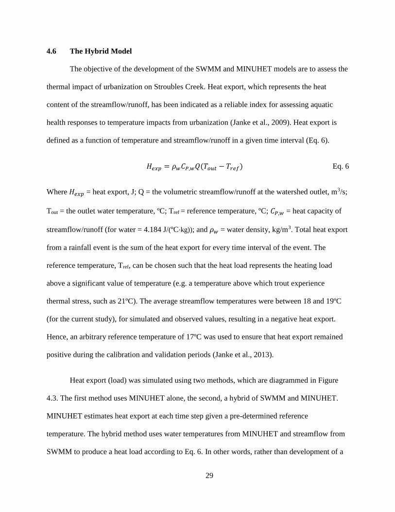
health responses to temperature impacts from urbanization (Janke et al., 2009). Heat export is
defined as a function of temperature and streamflow/runoff in a given time interval (Eq. 6).
𝐻𝑒𝑥𝑝 = 𝜌𝑤𝐶𝑃,𝑤𝑄(𝑇𝑜𝑢𝑡 − 𝑇𝑟𝑒𝑓) Eq. 6
Where 𝐻𝑒𝑥𝑝 = heat export, J; Q = the volumetric streamflow/runoff at the watershed outlet, m3/s;
Tout = the outlet water temperature, ºC; Tref = reference temperature, ºC; 𝐶𝑃,𝑤 = heat capacity of
streamflow/runoff (for water = 4.184 J/(ºC⋅kg)); and 𝜌𝑤 = water density, kg/m3. Total heat export
from a rainfall event is the sum of the heat export for every time interval of the event. The
reference temperature, Tref, can be chosen such that the heat load represents the heating load
above a significant value of temperature (e.g. a temperature above which trout experience
thermal stress, such as 21ºC). The average streamflow temperatures were between 18 and 19ºC
(for the current study), for simulated and observed values, resulting in a negative heat export.
Hence, an arbitrary reference temperature of 17ºC was used to ensure that heat export remained
positive during the calibration and validation periods (Janke et al., 2013).
Heat export (load) was simulated using two methods, which are diagrammed in Figure
4.3. The first method uses MINUHET alone, the second, a hybrid of SWMM and MINUHET.
MINUHET estimates heat export at each time step given a pre-determined reference
temperature. The hybrid method uses water temperatures from MINUHET and streamflow from
SWMM to produce a heat load according to Eq. 6. In other words, rather than development of a

30
de-coupled model (streamflows from SWMM input into MINUHET and then running
MINUHET), which is not feasible in MINUHET configuration, Eq. 6 was utilized to simulate
heat export based on SWMM outputs (streamflow) and MINUHET outputs (temperature).
Figure 4.3. Diagram of the heat export simulation methods.

31
Chapter 5.0 Comparison of SWMM, MINUHET, and Hybrid Models for the Stroubles
Creek Watershed
In this Chapter, the sensitivity of predicted streamflow to inputs to the MINUHET and
SWMM models was investigated. Downstream streamflow was then simulated using both the
SWMM and MINUHET models and the results were compared. The MINUHET model was also
employed to predict temperature downstream to evaluate the exceedance threshold temperature
for trout habitat. Lastly, heat loads were predicted by the MINUHET and hybrid models, and the
respective results were compared.
5.1 Sensitivity Analysis Results
A sensitivity analysis was conducted based on similar studies (Alamdari et al., 2017;
Xing et al., 2016) and the results are provided in Table 5.1. The average total streamflow volume
was most sensitive to imperviousness (Sr=0.380), followed by impervious depression storage
(Sr=-0.110), and subwatershed hydraulic width (Sr=0.030). The parameters in Table 5.1 are
ordered based on the absolute values of level of sensitivity, from high to low. Unlike similar
studies (Barco et al., 2008), the SWMM model of the Stroubles watershed was not very sensitive
to the Green-Ampt infiltration parameter (conductivity, Sr=-0.007). Likewise, it was also not
sensitive to Manning’s roughness for pervious and impervious surface and depression storage for
pervious lands.
The MINUHET Stroubles watershed model predicted water temperature exhibited a high
sensitivity to dew point temperature (Sr= 0.762, calculated from air temperature and relative
humidity) compared to other thermal parameters, such as heat capacity and thermal diffusivity of
pavements (Table 5.1). This was especially true during conditions free of large atmospheric or
ground heat fluxes, which commonly occur early in the morning. One of the key reasons that the
32
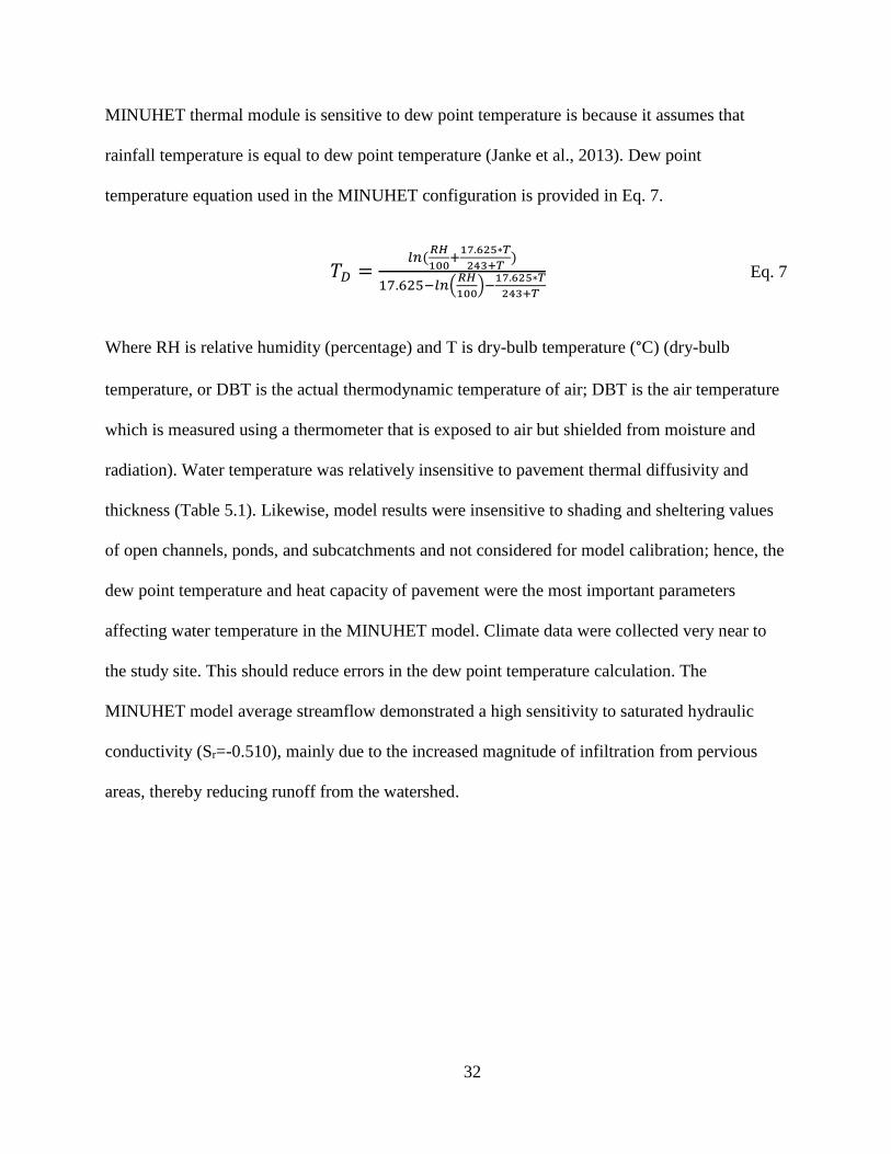
MINUHET thermal module is sensitive to dew point temperature is because it assumes that
rainfall temperature is equal to dew point temperature (Janke et al., 2013). Dew point
temperature equation used in the MINUHET configuration is provided in Eq. 7.
𝑇𝐷 =𝑙𝑛(
𝑅𝐻
100+
17.625∗𝑇
243+𝑇)
17.625−𝑙𝑛(𝑅𝐻
100)−
17.625∗𝑇
243+𝑇
Eq. 7
Where RH is relative humidity (percentage) and T is dry-bulb temperature (°C) (dry-bulb
temperature, or DBT is the actual thermodynamic temperature of air; DBT is the air temperature
which is measured using a thermometer that is exposed to air but shielded from moisture and
radiation). Water temperature was relatively insensitive to pavement thermal diffusivity and
thickness (Table 5.1). Likewise, model results were insensitive to shading and sheltering values
of open channels, ponds, and subcatchments and not considered for model calibration; hence, the
dew point temperature and heat capacity of pavement were the most important parameters
affecting water temperature in the MINUHET model. Climate data were collected very near to
the study site. This should reduce errors in the dew point temperature calculation. The
MINUHET model average streamflow demonstrated a high sensitivity to saturated hydraulic
conductivity (Sr=-0.510), mainly due to the increased magnitude of infiltration from pervious
areas, thereby reducing runoff from the watershed.
33
Table 5.1. Sensitivity coefficients of each parameter tested for the SWMM and MINUHET
models. Level of
Sensitivity
Parameter Sr
SWMM
High Imperviousness 0.380
Impervious depression storage -0.110
Hydraulic width 0.030
Pervious Manning roughness -0.008
Conductivity -0.007
Pervious depression storage -0.004
Low Impervious Manning roughness 0.001
MINUHET (Temperature)
High Dew point temperature 0.762
Heat capacity of pavements -0.023
Thermal diffusivity of pavements -0.009
Pavement thickness 0.008
Open channels degree of shading -0.002
Low Subwatersheds degree of shading -0.002
MINUHET (Streamflow)
Saturated hydraulic conductivity -0.510
5.2 Calibration and Validation for Streamflow
The sensitivity analysis (Section 5.1) assisted in identifying the most sensitive
parameters; this information was later used in developing sets of calibrated parameters, provided
in Tables B.1 and B.2 in Appendix B. As described in Table 2.1, there is a limited choice of
conductivity values for each subwatershed in MINUHET, as MINUHET only uses HSG
(Hydrologic Soil Group) categories for determination of each subwatershed soil hydraulic
conductivity. Hence, a specific hydraulic conductivity is attributed to each HSG category (based
on NRCS, SSURGO database and model calibration) (Table 5.2 and Figure 5.1f). The calibrated
parameter results are summarized in Table 5.2 for the MINUHET and SWMM models; a map of
each model by subcatchment is provided in Figure 5.1.

34
Table 5.2. SWMM and MINUHET hydrologic calibrated input parameters for simulating
streamflow. Parameters Unit Values range
SWMM
Percentage of impervious surfaces % 7.00-68.67
Total width of subcatchments m 72-1160
Subcatchments hydraulic conductivity mm/hr. 0.1-44.7
Impervious depression storage mm 2.5
Pervious Manning’s n - 0.218-0.388
Impervious Manning’s n - 0.008-0.014
MINUHET
Saturated hydraulic conductivity m/s HSG:B = 2.7×10⁻⁶
HSG:C = 1.8×10⁻⁶
After calibration, simulated streamflow matched the observed values well for the models
for both the calibration and validation periods. The goodness-of-fit results (model performance)
for the calibration and validation periods are summarized in Table 5.3. The simulated and
observed hydrographs for the calibration and validation periods are shown in Figure 5.2. As
shown in Table 5.3, SWMM provides a better estimate in terms of average percent difference
between observed and simulated streamflow. Judging from the relatively high values of NSE and
low values of PBIAS, the SWMM model was considered well calibrated and validated for
streamflow estimation at StREAM Lab (Table 5.3) monitoring location.
Table 5.3. Goodness-of-fit test results for assessing the reliability of calibration and validation
results of SWMM and MINUHET models for streamflow. Parameter SWMM MINUHET
Calibration Validation Calibration Validation
Model performance (hourly)
NSE 0.67(G*) 0.65(G) 0.62(S) 0.57(S)
R2 0.7(S*) 0.65(S) 0.65(S) 0.55(S)
RSR 0.58(S) 0.58(S) 0.61(S) 0.69(S)
PBIAS (% differences) -0.26%(G) -8.2%(G) -14.5%(G) -16.6%(S)
* G: Good; S: Satisfactory

35
Figure 5.1. Calibrated model parameters by subwatersheds, (a) Hydraulic conductivity for
SWMM (mm/hr.); (b) hydraulic width for SWMM (m); (c) Manning’s n (of impervious
portion) for SWMM; and (d) Manning’s n (of pervious portion) for SWMM; (e)
Imperviousness for SWMM; and (f) HSG by subwatersheds for MINUHET.

36
Since the value of PBIAS for SWMM is very close to zero during the calibration period,
the model appears to be reasonably accurate; however, the negative value of PBIAS during the
validation period indicates a slight overestimation bias. The R2 values of the calibration and
validation periods, 0.7 and 0.65, indicate that the model matches up well between simulated and
observed values. Evaluating model performance across events, the SWMM model predicted the
observed data set well during the calibration period (Figure 5.2a), but underpredicted streamflow
during high intensity storm events in the validation period, i.e., the storm events of July 5 and
September 29 (Figure 5.2b). This underprediction could possibly be due to the fact that our
criterion was to evaluate all streamflow, including baseflow and storm events, rather than
focusing strictly on storm events. Streamflow simulation using SWMM was considered
satisfactory by RSR index (Table 5.3)
Based on the values of NSE and PBIAS (Table 5.3), the MINUHET model was
considered satisfactorily calibrated and validated for streamflow. The negative value of PBIAS
during the calibration and validation periods indicates an overestimation bias. RSR is sufficiently
low to receive a satisfactory rating. Simulated and observed values for streamflow were
correlated, and R2 values of the calibration and validation periods were 0.65 and 0.55,
respectively. Model performance during the calibration and validation periods matched
streamflow of simulated and observed values reasonably well (Table 5.3). The MINUHET model
predicted the observed streamflow data set well during the calibration period, except for the first
15 days. This is likely due to dry antecedent conditions (Figure 5.3a). Furthermore, MINUHET
predicted streamflow reasonably well during intense events with less dry antecedent periods in
the validation period. Specifically, the verified simulation captured the peak streamflow
relatively well during the storm events of July 5 and September 29, 2015 (Figure 5.3b). Due to
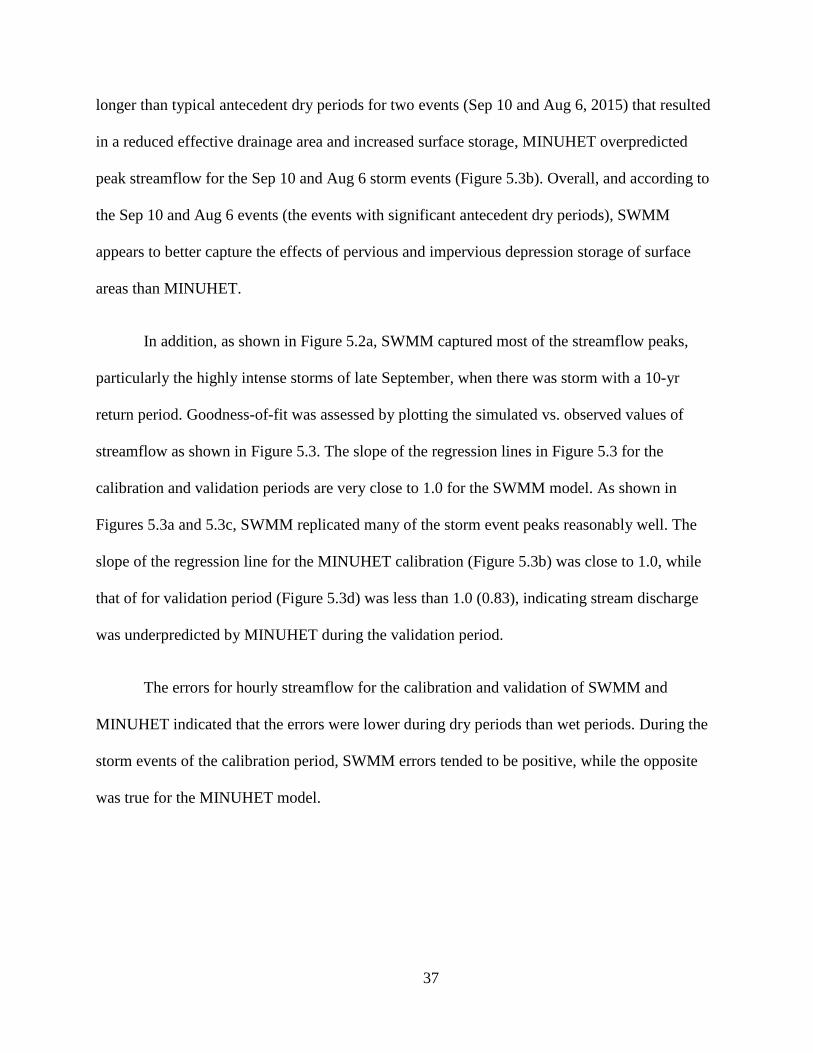
37
longer than typical antecedent dry periods for two events (Sep 10 and Aug 6, 2015) that resulted
in a reduced effective drainage area and increased surface storage, MINUHET overpredicted
peak streamflow for the Sep 10 and Aug 6 storm events (Figure 5.3b). Overall, and according to
the Sep 10 and Aug 6 events (the events with significant antecedent dry periods), SWMM
appears to better capture the effects of pervious and impervious depression storage of surface
areas than MINUHET.
In addition, as shown in Figure 5.2a, SWMM captured most of the streamflow peaks,
particularly the highly intense storms of late September, when there was storm with a 10-yr
return period. Goodness-of-fit was assessed by plotting the simulated vs. observed values of
streamflow as shown in Figure 5.3. The slope of the regression lines in Figure 5.3 for the
calibration and validation periods are very close to 1.0 for the SWMM model. As shown in
Figures 5.3a and 5.3c, SWMM replicated many of the storm event peaks reasonably well. The
slope of the regression line for the MINUHET calibration (Figure 5.3b) was close to 1.0, while
that of for validation period (Figure 5.3d) was less than 1.0 (0.83), indicating stream discharge
was underpredicted by MINUHET during the validation period.
The errors for hourly streamflow for the calibration and validation of SWMM and
MINUHET indicated that the errors were lower during dry periods than wet periods. During the
storm events of the calibration period, SWMM errors tended to be positive, while the opposite
was true for the MINUHET model.
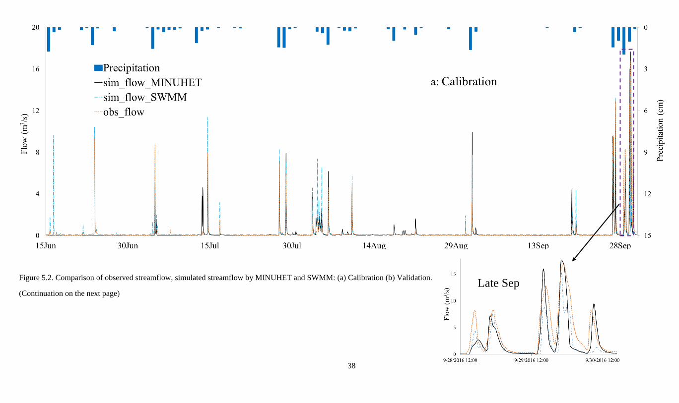
38
Figure 5.2. Comparison of observed streamflow, simulated streamflow by MINUHET and SWMM: (a) Calibration (b) Validation.
(Continuation on the next page)
Late Sep

39
July 5 Aug 6 Sep 10 Sep 29
40
Figure 5.3. Scatter plots of observed and simulated hourly streamflow: (a) Calibration for
SWMM; (b) Calibration for MINUHET; (c) Validation for SWMM; and (d) Validation for
MINUHET.
As is apparent in the scatter plots (Figure 5.3), some of the errors may be due to the
inability of the models to match streamflow peaks for some of the events. To analyze the error
data, the Shapiro-Wilk test was first conducted on the errors of simulated and observed discharge
(for calibration and validation steps), to see whether the errors are normally distributed. The p-
values of Shapiro-Wilk tests were obtained less than 0.05 for models, indicating the validation
and calibration errors were not normally distributed. Hence, a non-parametric Wilcoxon test
conducted to see if the medians of the errors obtained from SWMM and MINUHET were

41
significantly different from zero. According to the corresponding calculated p-values for SWMM
errors (for validation and calibration steps), the median of the errors was significantly different
from zero (<0.05), likely due to the storm events during wet periods, which resulted in higher
errors as compared to dry periods. Based upon the p-value for the MINUHET calibration
(<0.05), the median of the errors is also statistically different from zero. Regarding MINUHET
validation, The Wilcoxon test, which was conducted on the errors of MINUHET model (p-
value=0.44>0.05), indicates that the median streamflow errors may not be different from zero.
To further explore differences in predicted and observed discharge values for each model,
flow-duration curves (Figure 5.4) as cumulative frequency plots were developed. The observed
flow, simulated streamflow by SWMM, simulated streamflow by MINUHET, and baseflow (that
representing the groundwater contribution to streamflow) were plotted as shown on Figure 5.4.
Two-parameter filter method was used as the baseflow separation method in the current study to
generate baseflow and baseflow index (Figure 5.4); The description concerning Eckhardt method
is provided in Appendix D (Eckhardt, 2008). The flow-duration curves indicated that the
SWMM and MINUHET models simulated streamflow reasonably well during the calibration
period. During the calibration period (Figure 5.4a) and for small flows (less than 0.1 m3/s), the
SWMM simulation results were slightly greater than the observed discharges and MINUHET
simulations. As shown in Figure 5.4a, for MINUHET and observed results, the groundwater
contribution (which is assumed equal to baseflow) is the main source for streamflow when flows
are less than 0.05 m3/s, mainly because the groundwater discharge was an input. However,
simulated and observed flows less than 0.1 m3/s make up more than 80% of all flows. The
validated SWMM and MINUHET models resulted in lower agreement of observed and
simulated streamflow than during the calibration period (Figure 5.4b). However, simulation

42
using MINUHET experienced greater periods of streamflow >0.1 m3/s than SWMM and
observed flows.
Figure 5.4. Comparison of flow-duration curves of observed streamflow, simulated streamflow
by MINUHET, simulated streamflow by SWMM, and baseflow: (a) Calibration (b) Validation.
(a) Calibration
(b) Validation

43
Monthly variations of hourly streamflows for the summer were compared using a radar
plot (Figure 5.5). SWMM results appear to reflect a relatively better agreement with observed
streamflow than MINUHET during July and August for the calibration and validation periods.
The percentage difference between the simulated streamflow and the observed hourly mean
streamflow ranged from 1% to 25%, which may be classified as very good to relatively good
results (Al-Abed and Al-Sharif, 2008). The exception to this is in September; during which the
percent differences in hourly streamflows predicted by MINUHET were slightly lower than by
SWMM (for calibration and validation).
Figure 5.5. Analysis radar plot for hourly mean streamflow in each month; Val: Validation, Cal:
Calibration.
The calibrated and validated models were used to simulate streamflow for a total of ten
storm events, as listed in Table 5.4. Runoff fractions were calculated as the runoff depth

44
(volume) divided by rainfall depth (volume). During the less intense storm events of the
calibration period, the MINUHET model had a lower computed runoff fraction than SWMM. In
contrast, during larger storm events, the MINUHET model demonstrated much greater runoff
fractions than the SWMM model. Moreover, MINUHET had a better peak streamflow response
to the storm event of No. 5 (which was approximately a 10-yr rainfall event) than SWMM.
Overall, the SWMM model was a better predictor of runoff fraction than MINUHET model for
the calibration period. During all the storm events of the validation period (Table 5.4),
MINUHET resulted in far greater runoff fractions than the runoff fractions obtained from
observed data and SWMM model results. SWMM was closer to observed values of runoff
fraction for the validation period.
Table 5.4. Observed runoff fraction and predicted runoff fraction by SWMM and MINUHET, for
10 storm events, during the calibration and validation periods. Runoff Fraction
Storm No. Storm date Rainfall Intensity
(mm/hr.)
Rainfall
Depth (mm)
Observed SWMM MINUHET
Calibration
1 7/4/2016 5.9 29.50 0.17 0.14 0.13
2 7/14/2016 7.0 37.60 0.16 0.17 0.12
3 8/3/2016 1.2 39.60 0.13 0.31 0.25
4 8/31/2016 8.4 61.00 0.05 0.05 0.12
5 9/29/2016 3.5 73.15 0.71 0.37 0.63
Validation
6 7/5/2015 2.5 36.60 0.32 0.23 0.60
7 7/12/2015 1.7 43.70 0.12 0.16 0.18
8 8/10/2015 1.5 13.21 0.37 0.58 0.94
9 9/3/2015 1.3 11.18 0.02 0.04 0.01
10 9/29/2015 4.6 111.7 0.20 0.22 0.48
While storm events 8 and 9 were similar in terms of rainfall depth, storm event No. 9
resulted in a far lower runoff fraction than storm event No. 8 (Figure 5.6 and Table 5.4). The
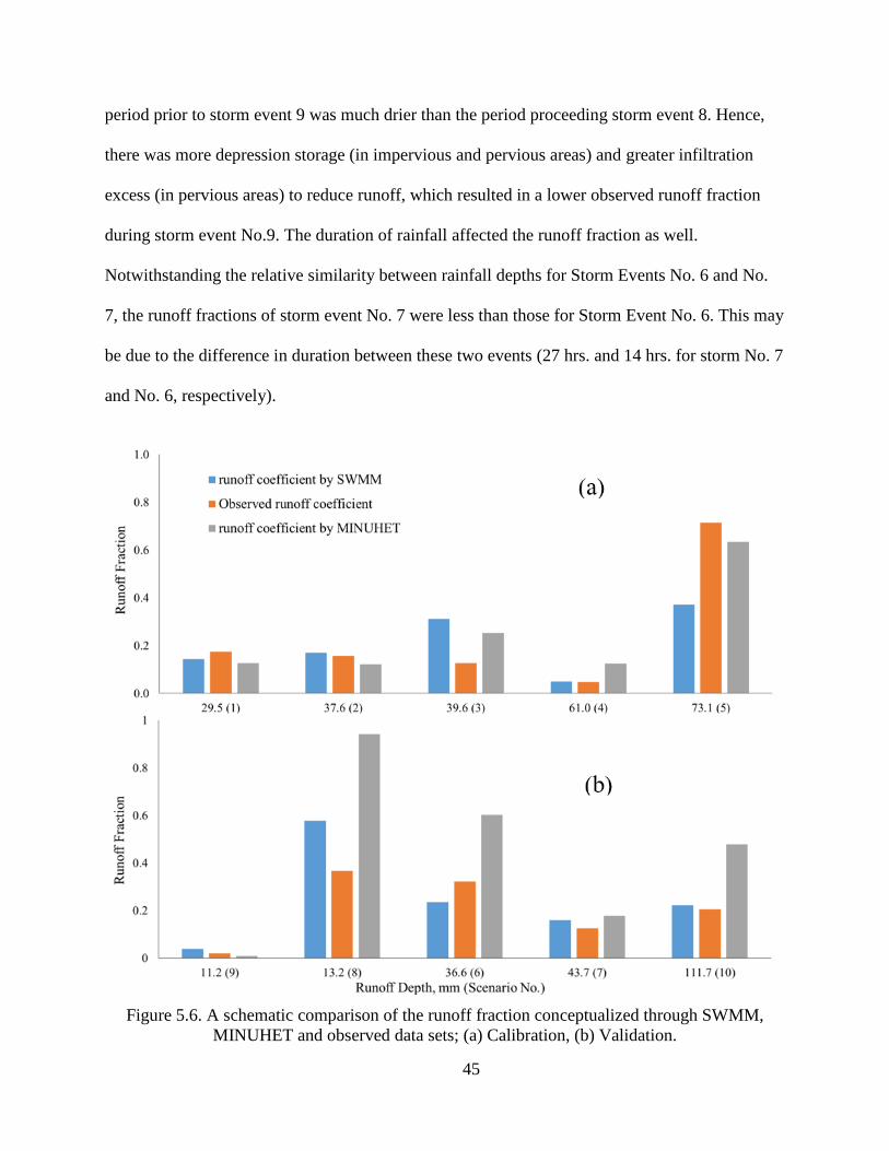
45
period prior to storm event 9 was much drier than the period proceeding storm event 8. Hence,
there was more depression storage (in impervious and pervious areas) and greater infiltration
excess (in pervious areas) to reduce runoff, which resulted in a lower observed runoff fraction
during storm event No.9. The duration of rainfall affected the runoff fraction as well.
Notwithstanding the relative similarity between rainfall depths for Storm Events No. 6 and No.
7, the runoff fractions of storm event No. 7 were less than those for Storm Event No. 6. This may
be due to the difference in duration between these two events (27 hrs. and 14 hrs. for storm No. 7
and No. 6, respectively).
Figure 5.6. A schematic comparison of the runoff fraction conceptualized through SWMM,
MINUHET and observed data sets; (a) Calibration, (b) Validation.

46
5.3 Temperature Simulation in the Watershed Downstream using MINUHET
Streamflow temperatures were simulated using MINUHET for the watershed
downstream. After calibration, the water temperature at the watershed outlet predicted by
MINUHET matched reasonably well with the observed values for the calibration and validation
periods. Goodness-of-fit results for water temperature for the calibration and validation periods
are summarized in Table 5.5 and the simulated and observed temperatures for the calibration and
validation periods are shown in Figure 5.7. In general, the simulation captures the overall
pattern/trend of the observed water temperatures. Additionally, the absolute value of percent
differences of simulated and observed mean temperature (PBIAS) for the calibration period is
greater than the validation period (Table 5.5), mainly due to the better prediction of water
temperature in the validation period.
Table 5.5. Goodness-of-fit test results for assessing the reliability of calibration and validation
results of MINUHET model for temperature, mean temperature of simulation and observation
for periods, and percent differences of simulation. Parameter Calibration Validation
Model Performance
NSE 0.55(S*) 0.58(S)
R2 0.70(S) 0.83(G**)
RSR 0.54(G) 0.68(S)
PBIAS (Percent differences) 5.60%(G) 4.80%(G)
Mean Water Temperature (°C)
Simulated 20.2 19.8
Observed 21.4 20.8
Average Daily Maximum Water Temperature (°C)
Simulated 22.0 21.8
Observed 24.0 23.7
Errors calculations (°C); Simulated-observed
Min error 0.0 0.0
Max error -5.48 -5.6
Mean error -1.16 -0.99
*S: Satisfactory; **G: Good

47
The MINUHET model was considered satisfactorily calibrated and validated for water
temperature based on NSE and PBIAS. The positive values of PBIAS during the calibration and
validation periods indicates an underestimation bias. RSR indicated a good calibration and
satisfactory validation. In terms of correlation, R2 values during the calibration and validation
periods were 0.70 and 0.83, or satisfactory and good performance, respectively. Surprisingly, the
model performed better in the validation period than in the calibration period, likely because for
the case study conditions, there is strong dependence (sensitivity) of simulated temperature to
dew point temperatures.
The factors driving the thermal regime in Stroubles Creek are illustrated by the storm
event of September 10, 2015. During the initial portion of the September 10 storm event (in the
afternoon), which had a significant antecedent dry period (Figure 5.7b), previously heated and
stored water in the Duck Pond was released to the stream. The Duck Pond is the largest pond in
the watershed in terms of surface area, and being downstream from most of the urbanized
watershed, is capable of capturing peak flows (Figure 4.1). However, during this event, a release
occurs as a result of the arrival of heated runoff from upstream impervious areas, which mixes
with and pushes out the stored, heated water in the Duck Pond, creating the second peak in
Figure 5.7b; the initial broad rise was due to diurnal temperature changes.
Water temperature at the watershed outlet was primarily influenced by dew point
temperature (according to sensitivity analysis results), except during large storm events. The
correlation between water temperature at the watershed outlet and dew point temperature is
strong during the beginning of high magnitude floods (e.g. September 29 of the validation
period), when there is significant surface runoff (Figure 5.7b). In this case, there is likely enough
surface runoff that any heat absorbed from the pavement is diluted by the large runoff volume
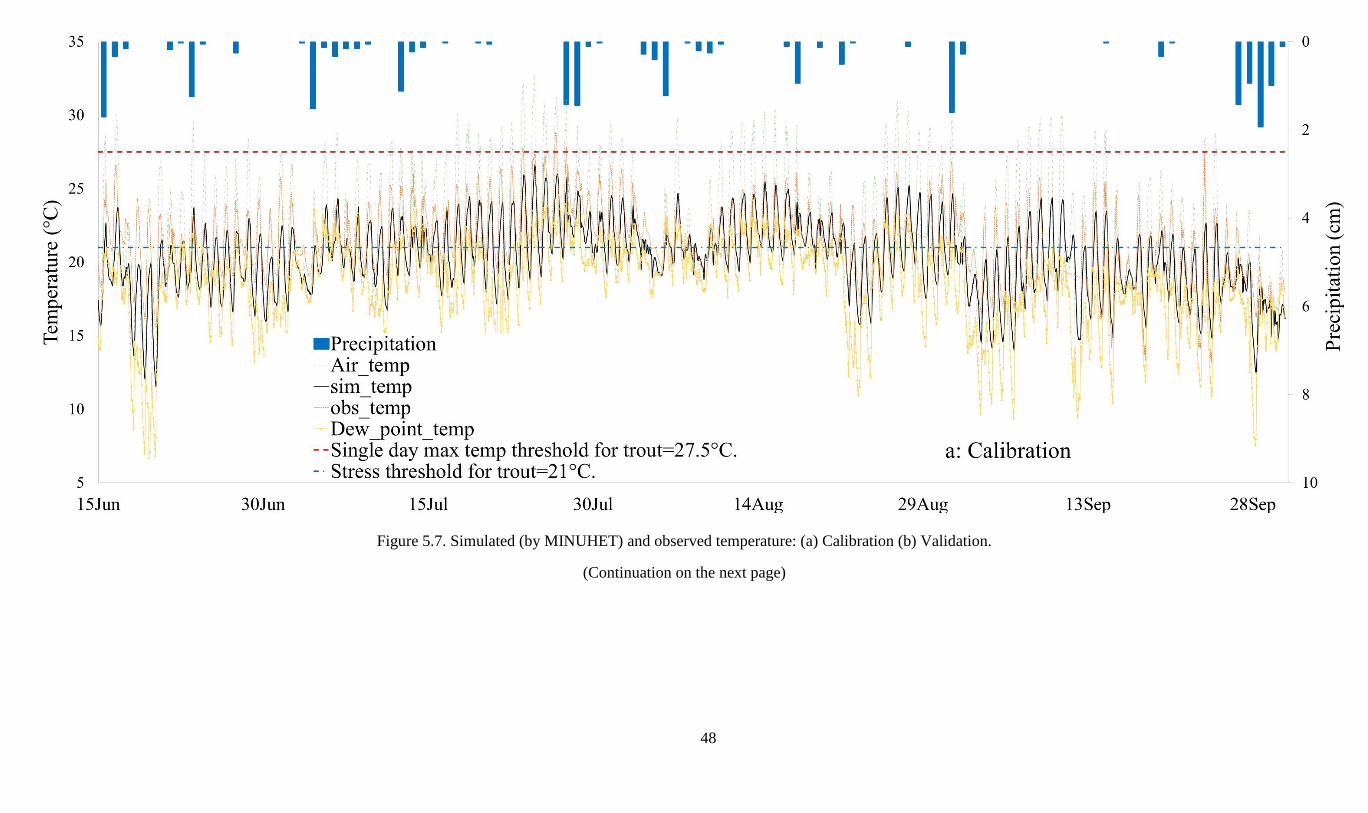
48
Figure 5.7. Simulated (by MINUHET) and observed temperature: (a) Calibration (b) Validation.
(Continuation on the next page)

49
(Continuation on the next page)
The graph of Sep 10 is
shown on the next page
The graph of Late Sep is
shown on the next page
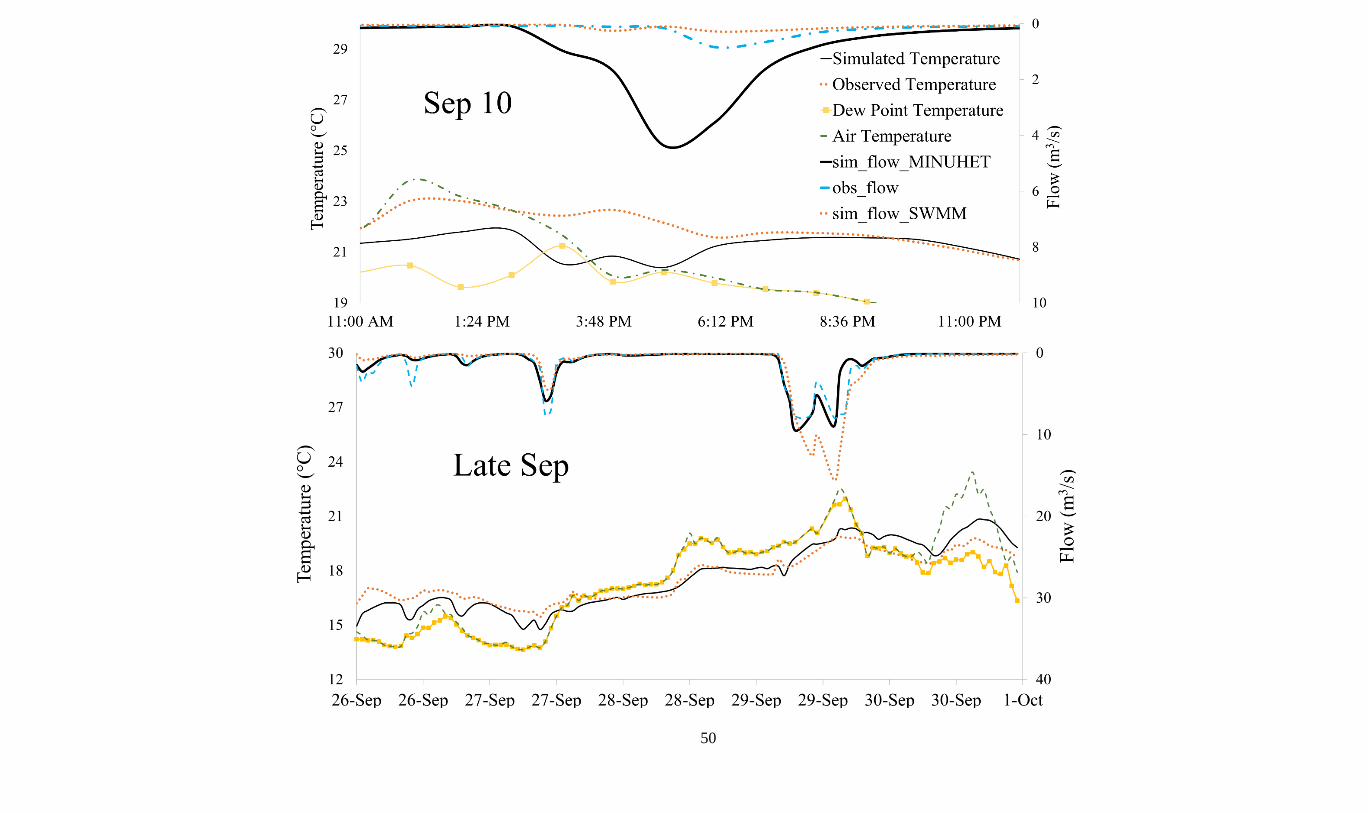
50
51
and is relatively unaffected by its temperature. In addition, as the rainwater falls, water
condenses and releases heat energy and the surface water (streamwater) temperature and air
temperature values become closer than dry period (as shown in the last three days of calibration
and validation periods, Figure 5.7). Overall, the dew point temperature and observed and
simulated temperatures match relatively better during flood (defined as high magnitude storm
events with runoff topping stream banks) compared to dry periods (Figure 5.7b). During floods,
the dew point temperature matches the air temperature well since the air is completely saturated
(Figure 5.7b). In contrast, during the initial hours of lesser magnitude storm events (Sep 27 of the
validation period), water temperature (simulated and observed) was well above dew point
temperature since water temperature during baseflow is strongly influenced by the groundwater
temperature which was warmer than the dew point temperature at that time (Figure 5.7b).
However, towards the end of the lesser magnitude storms, as most of the available heat was
absorbed from the ground surface by the runoff, water temperature at the watershed outlet tended
to approach dew point temperature, likely because the bulk of the streamflow towards the end of
the storm stems from surface water, rather than groundwater (Figure 5.7b).
Model performance was also assessed by plotting the simulated vs. observed values of
temperature as shown in Figure 5.8. Looking at calibration and validation graphs, the model
under-predicts water temperature at low temperatures, which are, presumably, baseflow
temperatures, likely because it is expected the baseflow to be warmer than stormflow in the
summer. In addition, for the calibration period, there seems to be two different sets of data. In
one set, the model is over-predicting and in the other instance, it is under-predicting. In other
words, there seems to be two “lines” of data at lower temperatures (these areas were highlighted
with black boxes). The slope of the regression line during calibration was 0.79, while the slope
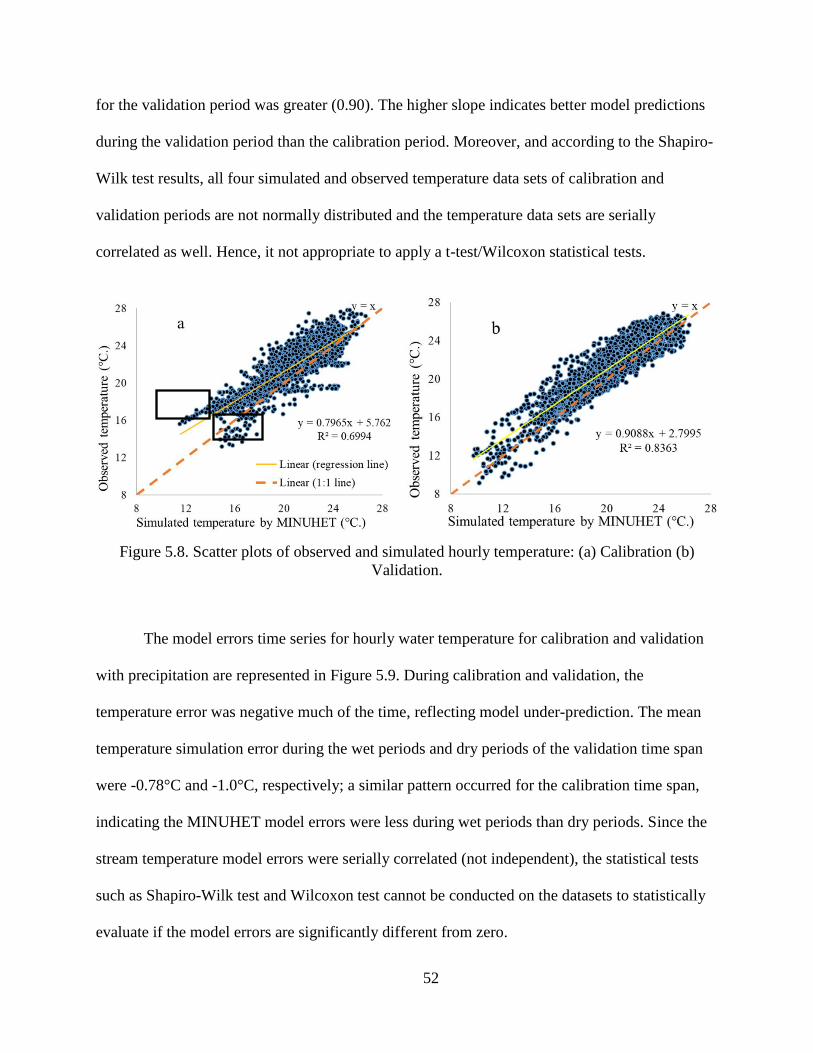
52
for the validation period was greater (0.90). The higher slope indicates better model predictions
during the validation period than the calibration period. Moreover, and according to the Shapiro-
Wilk test results, all four simulated and observed temperature data sets of calibration and
validation periods are not normally distributed and the temperature data sets are serially
correlated as well. Hence, it not appropriate to apply a t-test/Wilcoxon statistical tests.
Figure 5.8. Scatter plots of observed and simulated hourly temperature: (a) Calibration (b)
Validation.
The model errors time series for hourly water temperature for calibration and validation
with precipitation are represented in Figure 5.9. During calibration and validation, the
temperature error was negative much of the time, reflecting model under-prediction. The mean
temperature simulation error during the wet periods and dry periods of the validation time span
were -0.78°C and -1.0°C, respectively; a similar pattern occurred for the calibration time span,
indicating the MINUHET model errors were less during wet periods than dry periods. Since the
stream temperature model errors were serially correlated (not independent), the statistical tests
such as Shapiro-Wilk test and Wilcoxon test cannot be conducted on the datasets to statistically
evaluate if the model errors are significantly different from zero.

54
Figure 5.9. Model errors time series plot (simulated−observed) for hourly temperature, during calibration and validation periods.

55
To evaluate the effects of streamflow simulation on temperature simulation, temperature
error vs MINUHET streamflow error was plotted (Figure 5.10). Despite the errors in simulated
streamflow, the model generally predicted the overall pattern of stream temperature well. The
errors in stream temperature may be the result of errors in streamflow prediction, since errors in
the volume of streamflow could result in incorrectly modelled stream temperature, even if the
remaining heat fluxes are accurately simulated. The dominant processes controlling stream
temperature are advection (associated with streamflow during high flows), and surface heat
fluxes (during low flows). During high flows of the validation period when MINUHET
streamflow error was positive, temperature error tended to be negative (underestimation of
temperature), while during low flows and reduced streamflow errors, the opposite pattern was
observed (Figure 5.10).
Figure 5.10. Temperature error versus MINUHET streamflow error for the calibration and
validation periods.

56
Comparing the simulated versus observed values (Figure 5.8), it is apparent that the
simulation underestimated water temperature during calibration and validation periods; this
could be the result of any of the many assumptions made in the model. For example, errors in the
estimation of effective impervious area would affect partitioning of precipitation between surface
runoff and groundwater, resulting in errors in stream temperature predictions. Another
consideration was that Blacksburg is located at an elevation of ~670 m; however, the calculation
of dew point temperature, equation (Eq. 7), assumes standard atmosphere (i.e. sea level).
Although the input parameters of dew point temperature equation (air temperature and relative
humidity) were measured onsite (at the StREAM Lab meteorological station), for a given relative
humidity, the dew point temperature at sea level is approximately 2.4°C higher than at an
elevation of 670 m. This difference could be a source of systematic bias in the calculation of dew
point temperature.
The under-prediction of water temperature could have been the result of the model
assumption that the temperature of the precipitation was the dew point temperature. In reality,
water droplets condense high in the atmosphere (i.e. clouds) and only fall to the ground once the
droplets become large enough to overcome the force from the wind that keeps them in the air.
Since air temperature decreases with altitude/elevation, the air where the raindrops form is
significantly colder than the air below it. Hence, as the water droplets fall, they move through air
that is warmer than the air where they formed. Therefore, it would not be unreasonable to assume
that the temperature of the water droplets increases as they fall. In addition, as water vapor
condenses, it releases energy, which increases the air temperature. Thus, there may be many
reasons why the raindrops are likely warmer than the dew point temperature by the time they
reach the ground.

57
5.4 Implications for Trout Habitats
Trout toxicity threshold values of 27.5°C and 21°C are plotted in Figure 5.7 to assess the
impact of water temperature on aquatic health. Simulated water temperature exceeded the trout
stress threshold (21°C) during 39% and 38% of calibration and validation periods, respectively,
while the observed temperature exceeded the threshold 59% and 53% of the time for the
calibration and validation periods, respectively. Quantiles of simulated and observed hourly
stream temperatures representing the calibration and validation periods were developed (Table
5.6) to estimate how often water temperatures exceeded the trout stress threshold. Stream
temperature in summer is the most critical factor affecting production of trout (Selbig, 2015).
Each cell in Table 5.6 is shaded proportionately to increasing stress to trout as a function of
stream temperature. Trout mortality due to water temperature can occur outside of this standard,
as the degree of thermal stress outside of these tolerance ranges is a function of the rate and
exposure duration. Thus, restoration of the aquatic habitat of Stroubles Creek should consider
potential strategies to mitigate thermal pollution from impervious surfaces. An example of such
practices are bioretention cells, tree canopy restoration for increased shading of streams, and
installation of light-colored chip seal pavement.
Table 5.6. Quantile estimation of simulated hourly stream temperature compared to measured
stream temperature, for calibration and validation periods.
Percentile
1% 5% 10% 25% 50% 75% 90% 95% 99%
Calibration
Sim.** 14.0 15.9 17.0 18.7 20.3 21.8 23.3 24.1 25.2
Obs.*** 15.5 17.5 18.6 19.8 21.5 22.9 24.4 25.3 26.6
Validation
Sim. 11.3 14.7 15.8 18.1 20.2 21.9 23.2 24.1 25.3
Obs. 11.8 15.7 16.7 19.4 21.2 22.8 24.2 25.1 26.0
* Threshold maximum daily temperature for a seven-day exposure (>25.5°C), Initial thermal trout stress
(>21°C); **Sim. = Simulated streamflow temperature; ***Obs. = Observed streamflow temperature.
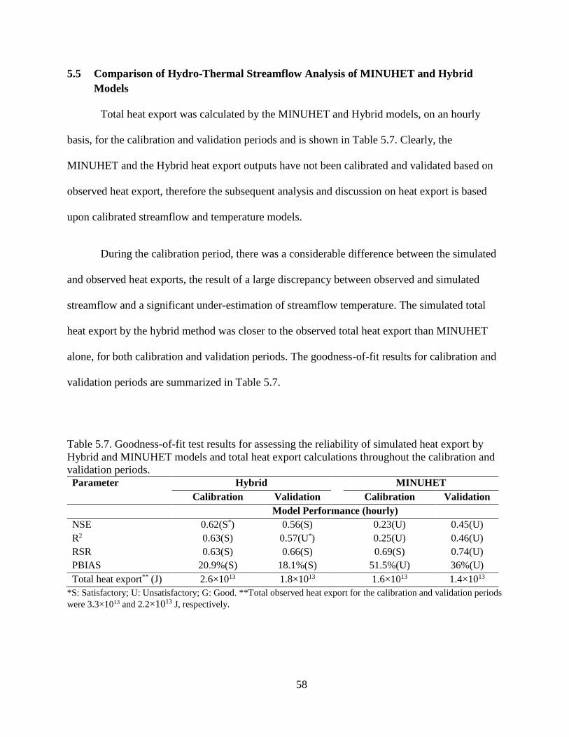
58
5.5 Comparison of Hydro-Thermal Streamflow Analysis of MINUHET and Hybrid
Models
Total heat export was calculated by the MINUHET and Hybrid models, on an hourly
basis, for the calibration and validation periods and is shown in Table 5.7. Clearly, the
MINUHET and the Hybrid heat export outputs have not been calibrated and validated based on
observed heat export, therefore the subsequent analysis and discussion on heat export is based
upon calibrated streamflow and temperature models.
During the calibration period, there was a considerable difference between the simulated
and observed heat exports, the result of a large discrepancy between observed and simulated
streamflow and a significant under-estimation of streamflow temperature. The simulated total
heat export by the hybrid method was closer to the observed total heat export than MINUHET
alone, for both calibration and validation periods. The goodness-of-fit results for calibration and
validation periods are summarized in Table 5.7.
Table 5.7. Goodness-of-fit test results for assessing the reliability of simulated heat export by
Hybrid and MINUHET models and total heat export calculations throughout the calibration and
validation periods. Parameter Hybrid MINUHET
Calibration Validation Calibration Validation
Model Performance (hourly)
NSE 0.62(S*) 0.56(S) 0.23(U) 0.45(U)
R2 0.63(S) 0.57(U*) 0.25(U) 0.46(U)
RSR 0.63(S) 0.66(S) 0.69(S) 0.74(U)
PBIAS 20.9%(S) 18.1%(S) 51.5%(U) 36%(U)
Total heat export** (J) 2.6×10¹³ 1.8×10¹³ 1.6×10¹³ 1.4×10¹³
*S: Satisfactory; U: Unsatisfactory; G: Good. **Total observed heat export for the calibration and validation periods
were 3.3×10¹³ and 2.2×10¹³ J, respectively.

59
The hybrid model can be considered satisfactorily calibrated and validated for estimation
of heat export based on NSE and R2 (Table 5.7). In contrast, the MINUHET model shows poor
agreement and correlation between simulated and observed heat export for the calibration period
(low NSE and R2), with improved agreement and correlation for the validation period (i.e.
greater NSE and R2 compared to the calibration period). The improved model predictions during
the validation period are likely due to the better water temperature predictions in the validation
period, as compared to the calibration period. RSR is satisfactory for the hybrid model for
calibration and validation; however, MINUHET did not perform satisfactorily for the validation
period. The PBIAS positive values indicate that the MINUHET and the Hybrid models under-
predicted observed total heat exports (Figure 5.11).
Goodness of fit for the Hybrid model was assessed by plotting the simulated vs. observed
values of heat export as shown in Figure 5.12. The slope of the regression line during validation
was very close to 1.0, while that of for calibration period was greater (1.24). It shows that the
two data sets (during the calibration period) may be slightly different from zero, compared to the
validation period. Overall, predicting heat export by the Hybrid method was better than
simulating heat export by MINUHET alone (Table 5.7, Figures 5.11 and 5.12).
The radar plot of hourly mean heat export for the summer months (Figure 5.13) indicates
that the Hybrid model results in lower percent differences than MINUHET during July and
August for both calibration and validation periods. The percentage difference between the
simulated hourly mean heat export and the observed hourly mean heat export ranged from 7% to
35%, which may be classified as very good to poor (Al-Abed and Al-Sharif, 2008). Heat export
for September simulated by MINUHET and Hybrid was far less than the observed values for

60
Figure 5.11. Comparison of hourly heat export simulation by MINUHET and Hybrid models: (a) Calibration (b) Validation (heat export unit is Watt as it defined to the energy consumption rate of one
joule per second

61
Figure 5.12. Scatter plots of observed and simulated (by Hybrid) heat export: (a) Calibration (b)
Validation.
Figure 5.13. Analysis radar plot for hourly mean heat export in each month, for calibration and
validation periods; val: Validation, cal: Calibration.

62
both calibration and validation periods. This likely stems from MINUHET’s under-predicting
water temperature in September, for calibration and validation periods.
It is apparent that the heat export simulation by Hybrid underestimated observed heat
export during calibration and validation periods. The existing percentage difference value
(PBIAS) between observed and simulated heat export by the Hybrid model (Table 5.7) may be
due to the existing relatively long open channels (Stroubles Creek) in the watershed, and the
aforementioned uncertainties in simulating streamflow in MINUHET. Since MINUHET does not
model open channel thermal processes, simulated water temperature at the outlet of the
watershed may have some uncertainties and error. Another consideration is using all streamflow
rather than storm events to simulate streamflow by SWMM, which resulted in underestimation of
observed streamflow peaks (because SWMM was mainly developed to simulate storm events);
Hence, simulation using Hybrid model underestimated observed heat export, and can be
considered as a relatively non-conservative model.
MINUHET was applied to a simple, small watershed and predicted total heat export with
error less than 15% (Janke et al., 2013). In this study, with a much more complex and larger
watershed, the error was larger. The Hybrid model resulted in better percent differences of total
heat export than MINUHET, for calibration and validation periods (Table 5.7). The percent
differences for heat export obtained by the Hybrid model were approximately similar to the
values simulated by MINUHET in the Janke et al., (2013) study. This suggests using the Hybrid
model of SWMM and MINUHET for complex urban watersheds, would likely result in better
agreement between observed and simulated heat export than MINUHET alone.
63
5.6 Simulating Temperature and Heat Loads at the Watershed-Scale
The temperature and heat export results of the calibrated MINUHET and the Hybrid
models were plotted based upon respective values at the outlet of each subwatershed (Figure
5.14). Based on these plots, two storms (Table 5.8) were selected from the validation period to
assess the impact of storm events antecedent dry periods (ADPs) on temperature and heat load
simulation and the ability of MINUHET and Hybrid models in simulation of temperature and
heat load, respectively, in watershed-scale, with regards to imperviousness percentage of each
subwatershed. These two were the only storms of the validation period that produced runoff at
the all subwatershed outlets during the simulation by both MINUHET and SWMM, and these
storms had the shortest and longest antecedent dry periods (ADPs). Thus, they were selected for
maximum contrast (Table 5.8).
Mean temperature at the outlet of each subwatershed (MTOES) for each storm was
compared to assess each models’ capabilities at a range of ADPs and air temperatures. The
Shapiro-Wilk test was conducted on each data sets of MTOES to check for normality; p-values
were less than 0.05, thus the data do not appear to be normally distributed. Hence, the Wilcoxon
test was used to compare the median ranks of each data set; p-values were less than 0.05,
indicating that the median temperature of subwatershed data sets for the two storms was
significantly different (Table 5.8). The simulated mean/average temperature of all subwatersheds
outlet runoff for the Aug 11 storm was greater than that of storm Sep 29 due to greater ADP
(which led to greater absorbed heat from the pavement), greater mean air temperature, and less
surface runoff volume (Table 5.8). The Sep 29 storm experienced only 2 days of ADP, while
ADP was 28 days for the Aug 11 storm. The Sep 29 storm produced far greater runoff than Aug
11 storm, which consequently resulted in greater total heat export.

64
The temperature, heat export, and imperviousness maps of the watershed for the Sep 29
and Aug 11 storms of summer 2015 are provided in Figure 5.14. The red colors of the
temperature and heat export maps of each subwatershed represent the respective values at the
outlet of each subwatershed. Since MINUHET was mainly developed to simulate urbanized
watersheds, and the central and eastern sections of the urbanized portion of watershed are highly
urbanized (Figure 5.14e), the urbanized portion of watershed imperviousness pattern corresponds
relatively well with the temperature map of Sep 29 storm (simulated by MINUHET) as shown in
Figure 5.14a.
The temperature map of the downstream portion of the Stroubles Creek Watershed during
Sep 29 storm is not consistent with the imperviousness map (Figures 5.14a and e), due to the
mitigating effects of agricultural and forestry land cover downstream. The heat export maps
(simulated by the Hybrid model) of Sep 29 and Aug 11 events (Figures 5.14b and d) are
approximately consistent with the imperviousness map (Figure 5.14e) at the watershed-scale; this
may be due to the more accurate simulation of runoff at each subwatershed outlet by SWMM.
The temperature map of Aug 11 storm (Figure 5.14c) does not match Figure 5.14e, possibly
because there is far less runoff at the subwatershed outlets in the Aug 11 than the Sep 29 event,
resulting in uncertainties in temperature simulation.
Overall, MINUHET and the hybrid models can be considered reliable indexes/models in
developing the temperature and heat export maps of urbanized watersheds, respectively, during
large storm events.

65
Table 5.8. Hydrologic and thermal characteristics of the selected storms for the validation period.
Parameter Storms Date
9/29/2015 8/11/2015
Intensity (mm/hr.) 9.46 5.10
ADP* (day) 2 28
Mean air temperature during ADP (°C) 18.24 21.57
Total Precipitation (mm) 108.71 13.20
Total runoff volume (m3) 1.37×10⁵ 1.65×10⁴
Simulated Mean temperature** (°C) 19.16 20.33
Total heat export by Hybrid model (J) 1.04×10¹² 2.46×10¹¹
P-value of Shapiro-Wilk test for temperature at the subwatersheds outlets <0.05 <0.05
P-value of Wilcoxon test for the temperatures of storms <0.05
*Antecedent Dry Period; **Mean temperature of all subwatersheds runoff.

66
Figure 5.14. Temperature, heat export and imperviousness maps of Stroubles Creek
subwatersheds: (a) Temperature map for Sep 29 storm, (b) Heat export map for Sep 29 storm, (c)
Temperature map for Aug 11 storm, (d) Heat export map for Aug 11 storm, and (e)
Imperviousness coefficients map.
67
Chapter 6.0 Utilizing Watershed-Scale Practices/Approaches to Mitigate Thermal Effects
In this chapter, the calibrated and validated SWMM and MINUHET models presented in
Chapter 5 were utilized to apply watershed-scale infiltration practices and thermal mitigation
approaches to reduce temperature and heat loads at the watershed outlet. Bioretention, various
modified conventional pavements/roofing materials (referred to as “cool surfaces”), and
increased vegetation canopies were used individually in a number of scenarios with the objective
of mitigating predicted thermal pollution during the validation period (Summer 2015).
6.1 Cooling Effects of Various Pavements and Roofs Installation
Impervious conventional pavements consisting of either concrete and asphalt increase the
peak surface temperature to 48-75°C (Ferguson et al., 2008). During daylight, heat builds and
propagates downward in the pavement to the subsurface; this heat is later released as radiative
heat during the night. Higher temperature pavements surfaces transfer this heat to runoff, which
is discharged to local water bodies. In addition to pavements, residential and commercial roofs
contribute to increased heat load of surface runoff. Urban runoff causes a host of aforementioned
water quantity and quality issues in receiving streams (Walsh et al., 2005), including excessive
temperatures which impair aquatic life (Li et al., 2013). Pavement and roof properties control the
rate of heat absorption and are critical in mitigating hot pavements. Modified or “cool
pavements/roofs” reflect solar radiation and lower the surface temperature when compared to
unmodified conventional pavements/roofs.
A newly installed concrete pavement has a high magnitude solar reflectance which is
generally considered as cool pavements (Mohegh et al., 2017). The albedo of a specific surface is
the percentage of solar energy reflected by that surface. In addition to the pavement surface type,
the albedo of the pavement affects its temperature below the pavement surface, since less heat is

68
available at the surface to be transferred downward. Concrete and asphalt conventional
pavements have an approximate initial albedo of 5 and 35%, respectively (at the beginning of
construction) (Ferguson et al., 2008). This is what these materials are assigned in MINUHET.
Over time, use of the surfaces for foot and vehicle traffic dirty the cement causing it to darken
during the life time of concrete pavement, gradually lowering the albedo; in contrast to concrete,
asphalt tends to lighten as the binder oxidizes and the aggregate is exposed to weathering, which
leads to higher albedo over time (Figure 6.1). Therefore, the actual albedo depends on pavement
material and age (Ferguson et al., 2008). Generally, lighter pavements tend to have greater
albedo, affecting surface temperatures considerably (Mohegh et al., 2017).
Thermal emittance of a surface is the radiant energy at a specific temperature per unit
area. Unlike albedo, which is mostly dependent on color, thermal emittance correlates with
surface material type and properties (Ferguson et al., 2008). Solar reflectance which is a term
used for visible spectrum is an index representing effects of both albedo and thermal emittance
combined. In addition, pavement thickness indicates how much heat is stored in a pavement,
with thicker pavements storing more heat (Herb et al., 2009b). The typical unit of heat capacity
is J/kg·°C, but MINUHET models heat capacity unit is in J/m3·°C; hence the density of each
material must be considered to compute the approximate heat capacity of each material (Table
6.1) (Ferguson et al., 2008; Herb et al., 2010).

69
Figure 6.1. Asphalt and concrete pavements typical albedo over time (Ferguson et al., 2008)
Asphalt and concrete pavement types and commercial and residential rooftops are the
dominant impervious surface types of the Stroubles Creek Watershed, which were used as input
to the watershed module of MINUHET model. There is a limitation in MINUHET configuration,
as there is no option to divide an impervious area of a subwatershed into various impervious land
uses mentioned above. Hence, the designer has to choose only one of the aforementioned
impervious land uses for each subwatershed as the dominant impervious surface type (Figure
6.2a); this could be a source of systematic bias in heat load simulation. The current dominate
condition of the impervious surface type of each subwatershed is shown in Figure 6.2a (based on
aerial imagery, field review, and Town of Blacksburg GIS layers information). After MINUHET
calibration, various types of pavement and roofing materials were installed in the watershed
through the calibrated MINUHET configuration to evaluate temperature and heat load variations
downstream. Lastly, a combination of utilizing cool pavements installation and cool roofing
materials (at the watershed-scale) was simulated in two individual scenarios to maximize heat
load and temperature reduction downstream (Figure 6.1d, and scenarios 9 and 10 shown on
Table 6.1).
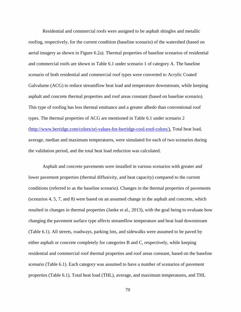
70
Residential and commercial roofs were assigned to be asphalt shingles and metallic
roofing, respectively, for the current condition (baseline scenario) of the watershed (based on
aerial imagery as shown in Figure 6.2a). Thermal properties of baseline scenarios of residential
and commercial roofs are shown in Table 6.1 under scenario 1 of category A. The baseline
scenario of both residential and commercial roof types were converted to Acrylic Coated
Galvalume (ACG) to reduce streamflow heat load and temperature downstream, while keeping
asphalt and concrete thermal properties and roof areas constant (based on baseline scenario).
This type of roofing has less thermal emittance and a greater albedo than conventional roof
types. The thermal properties of ACG are mentioned in Table 6.1 under scenario 2
(http://www.berridge.com/colors/sri-values-for-berridge-cool-roof-colors/). Total heat load,
average, median and maximum temperatures, were simulated for each of two scenarios during
the validation period, and the total heat load reduction was calculated.
Asphalt and concrete pavements were installed in various scenarios with greater and
lower pavement properties (thermal diffusivity, and heat capacity) compared to the current
conditions (referred to as the baseline scenario). Changes in the thermal properties of pavements
(scenarios 4, 5, 7, and 8) were based on an assumed change in the asphalt and concrete, which
resulted in changes in thermal properties (Janke et al., 2013), with the goal being to evaluate how
changing the pavement surface type affects streamflow temperature and heat load downstream
(Table 6.1). All streets, roadways, parking lots, and sidewalks were assumed to be paved by
either asphalt or concrete completely for categories B and C, respectively, while keeping
residential and commercial roof thermal properties and roof areas constant, based on the baseline
scenario (Table 6.1). Each category was assumed to have a number of scenarios of pavement
properties (Table 6.1). Total heat load (THL), average, and maximum temperatures, and THL

71
reduction (compared to baseline scenario) were simulated for each of eight scenarios during the
validation period (Table 6.2). Since asphalt and concrete have similar thermal emittance, the
thermal emittance of both asphalt and concrete pavements was kept constant at a value of 91%
(https://heatisland.lbl.gov/). Thermal diffusivity is the thermal conductivity of a pavement, which
ranges from 5×10⁻⁷ to 30×10-7 m2/s within MINUHET (Table 6.1). Pavement thickness is
required to be at least 15 cm for semi-heavy traffic areas to meet structural stability (Iowa storm
water management manual, 2008; Ketabchy et al., 2016b). The current MINUHET model input
for asphalt and concrete pavement thickness was assumed to be 20 cm based on requirements for
design standards of streets for Blacksburg, VA (Moore et al., 2016; Wakchaure et al., 2001).
Heat loads and temperature values of pavement and roof surfaces and percentage of time
that temperature exceeded the 21°C threshold (PTTET) for each are provided in Table 6.2.
Concrete pavement showed better performance in reducing mean temperature and total heat load
compared to asphalt pavements (Table 6.2 and Figure 6.3). The albedo coefficient of concrete is
far greater than asphalt (Table 6.1), resulting in lower total heat loads in all pavement scenarios.
Thermal diffusivity is the rate of heat conductivity of pavement, and greater thermal diffusivity
results in more heat energy transferred between the hot side and cold side of a pavement, thereby
storing less heat energy through the pavement surface (which is exposed to stormwater) (Li et
al., 2013). Specific heat capacity of pavements are less than wet soil and greater than dry soil
(https://www.engineeringtoolbox.com/specific-heat-solids-d_154.html); therefore, build-up areas
capture more thermal energy than undeveloped areas covered by dry soil. Hence, scenarios with
higher specific heat capacity of pavements resulted in less stored heat (scenarios 4 and 7 of
Tables 6.1 and 6.2). The sensitivity analysis results of thermal diffusivity and heat capacity
mentioned in Table 5.1 confirm these results.

72
Figure 6.2. The dominant impervious surface type of each subwatershed as input to the
MINUHET model for (a) Current condition or baseline scenario of watershed (based on aerial
imagery, field review, and Town of Blacksburg GIS layers information), (b) Scenarios of
Category B, (c) Scenarios of Category C (based on Table 6.1), and (d) scenarios of Category D
(based on Table 6.1). Legends of (b) and (c) Figures are similar to that of (a).

73
Table 6.1. The properties of pavements and roofs, which are used as input to the MINUHET model, based on 10 scenarios. Scenario No. Albedo (%) Thermal Emittance (%) Surface Roughness* Thermal Diffusivity (m2/s) Thickness (m) ~ Value of Heat Capacity (J/m3·°C)
Category A: scenarios of roof surfaces
1** RR***: 15
CR***: 30
RR: 94
CR: 70
RR: 0.010
CR: 0.010
RR: 10.0×10⁻⁷
CR: 04.2×10⁻⁶
RR: 0.01
CR: 0.02
RR: 3.0×10⁶
CR: 3.0×10⁶
2 67 (H****) 0.20 (L****) 0.010 9.7 × 10⁻⁵ (H) 0.02 3.0×10⁶
Category B: 100% of roadways, streets, parking lots, and sidewalks paved by asphalt
3** 5 91 0.013 10×10-7 0.20 3.0×10⁶
4 5 91 0.013 15×10-7 (H) 0.20 4.0×10⁶ (H)
5 5 91 0.013 5×10⁻⁷ (L) 0.20 1.5×10⁶ (L)
Category C: 100% of roadways, streets, parking lots, and sidewalks paved by concrete
6** 35 91 0.011 10×10-7 0.20 3.0×10⁶
7 35 91 0.011 15×10-7 (H) 0.20 4.0×10⁶ (H)
8 35 91 0.011 5×10⁻⁷ (L) 0.20 1.5×10⁶ (L)
Category D: scenarios 2 and 7 were combined for all roof and pavement surfaces of watershed
9 GR***: 67
CP***: 35
GR: 20
CP: 91
GR: 0.010
CP: 0.011
GR: 9.7 × 10⁻⁵
CP: 15×10-7
GR: 0.02
CP: 0.20
GR: 3.0×10⁶
CP: 4.0×10⁶
10***** GR***: 67
CP***: 25
GR: 20
CP: 91
GR: 0.010
CP: 0.011
GR: 9.7 × 10⁻⁵
CP: 15×10-7
GR: 0.02
CP: 0.20
GR: 3.0×10⁶
CP: 4.0×10⁶
*based on Herb et al. 2010 and Rossman, 2009
**represents the current properties of roofs/pavement, or baseline scenario of pavements/roofs properties;
***RR: Residential Roof; CR: Commercial Roof; GR: Galvalume Roof; CP: Concrete Pavement
****H: Higher than baseline scenario; L: Lower than baseline scenario.
***** Scenario 10 represents assumption of 6-year concrete age, while scenario 9 assumed concrete pavement newly constructed.

74
Scenario 7 resulted in the lowest total heat and water temperature between all scenarios
of asphalt and concrete pavements. Scenario 7 showed better performance of urban heat island
effect reduction compared to other scenarios. Overall, solar reflectance was the most critical
parameter concerning how pavements interact thermally with the environment when exposed to
stormwater, radiation and sunlight; thermal diffusivity and heat capacity of pavements count as
second order factors (Iowa storm water management manual, 2008). Scenario 5 (asphalt
pavement) resulted in increased heat load compared to scenario 0 (Current Condition) since
thermal diffusivity and heat capacity increased. Scenario 8 (concrete pavement) resulted in lower
heat reduction compared to scenarios 6 and 7, since the aforementioned thermal properties
increased. Surprisingly, all concrete and asphalt scenarios performed similar in simulating
maximum temperature of streamflow during the validation period, while PTTET of concrete
scenarios were approximately 3% less than asphalt scenarios (Table 6.2 and Figure 6.3).
ACG was used as surface type for both commercial and residential roofs. ACG
installation considerably reduced heat load of the watershed during validation period (-35.6%, as
shown on Table 6.2 as scenario 2). Greater albedo, less thermal emittance (greater solar
reflectance combined), and far greater thermal diffusivity compared to current condition of roofs
resulted in better performance of heat reduction and PTTET (Table 6.2).
Pavements and roofs scenarios with the best performance (scenarios 2 and 7) were
combined at the watershed-scale to minimize thermal pollution downstream, thus creating
scenarios 9 and 10 (Table 6.1). Installations of ACG for roofs material and concrete for
pavement were utilized to evaluate heat load and temperature downstream. Scenario 9,
representing newly-constructed concrete pavements, resulted in 46% and 4.5% reduction in heat
load and Percentage of Time Temperature Exceeded 21°C Threshold (PTTET), respectively

75
(compared to baseline scenario), which were greater than using either concrete pavement or
ACG alone. Concrete pavement with 6 years of age assessed and used in scenario 10 to evaluate
effect of pavement age on heat load of watershed (Tables 6.1 and 6.2). According to Ferguson et
al. 2008, the albedo of concrete pavements declines by 25%, 6 years after construction (Figure
6.1). Hence, scenario 10 assumed concrete pavement to have an age of 6 years, thereby resulting
in less reduction of total heat load than scenario 9 (which assumed concrete pavement was
newly-constructed) (Figure 6.3).
Table 6.2. Heat load and temperature values of cool roof and pavement installation scenarios, at
the outlet of the watershed, during the validation period. Scenario
No.
Total Heat
Load (J)
Heat Red.*
(%)
Mean
Temperature (°C)
Maximum
Temperature (°C)
PTTET
(%)
0*** 1.40×10¹³ - 19.83 25.76 37.90
1 1.40×10¹³ - 19.83 25.76 37.90
2 9.04×10¹² -35.60 18.93 25.76 34.88
3 1.40×10¹³ ~00.00 19.83 25.76 37.90
4 1.40×10¹³ -00.38 19.82 25.74 37.82
5 1.42×10¹³ 01.05 19.84 25.76 37.90
6 1.28×10¹³ -8.54 19.22 25.75 35.57
7 1.24×10¹³ -11.40 19.08 25.48 35.34
8 1.33×10¹³ -05.22 19.69 25.75 37.44
9 7.56×10¹² -46.10 18.71 25.72 33.73
10 8.41×10¹² -39.75 18.84 20.78 34.53
*Heat load percentage reduction compared to baseline scenario (reference temperature for heat load calculations is
17°C). The negative values represent heat load reduction while the positive values represents increased heat load;
**threshold for trout; ***this scenario represents the Current Condition or baseline scenario of the watershed.
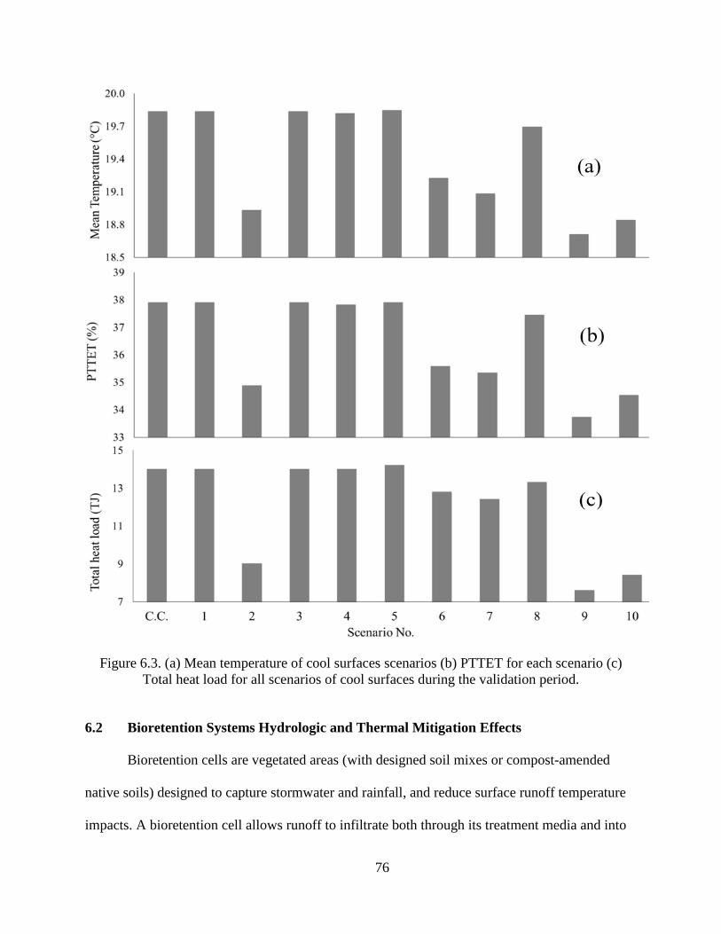
76
Figure 6.3. (a) Mean temperature of cool surfaces scenarios (b) PTTET for each scenario (c)
Total heat load for all scenarios of cool surfaces during the validation period.
6.2 Bioretention Systems Hydrologic and Thermal Mitigation Effects
Bioretention cells are vegetated areas (with designed soil mixes or compost-amended
native soils) designed to capture stormwater and rainfall, and reduce surface runoff temperature
impacts. A bioretention cell allows runoff to infiltrate both through its treatment media and into

77
the native soil beneath it; this infiltrated water provides recharge for the shallow water table.
Bioretention is a stormwater BMP that can moderate mean runoff temperature, i.e., keeping it
cool in seasonally hot weather and prevents severe temperature fluctuations during cold months
(Herb et al., 2010). This section evaluates the effectiveness of bioretention cells in reducing heat
load and temperature through installation of bioretentions systems at the down-gradient end of a
number of selected parking lots using the calibrated SWMM and MINUHET models. Schematic
of a bioretention cell is shown in Figure 6.4.
Figure 6.4. Schematic of a bioretention cell (Rossman, 2009).
Based on a specified bioretention system volume, depression storage is increased in the
pervious part of the subwatershed (extra depressional storage = bioretention volume/pervious
area). Bioretention cells were simulated in SWMM using the specific attributes listed in Table
6.3. Infiltration ponds were used instead of bioretention in the MINUHUET model because: 1) in
the current configuration of MINUHET, only rooftops can be routed to a bioretention cell, while,
in our watershed, the main portion of the impervious area is pavement; 2) Since infiltration
ponds are external to a subwatershed within MINUHET, they are defined individually, which is
similar to the SWMM approach; 3) There is a software issue in the data entry for bioretention
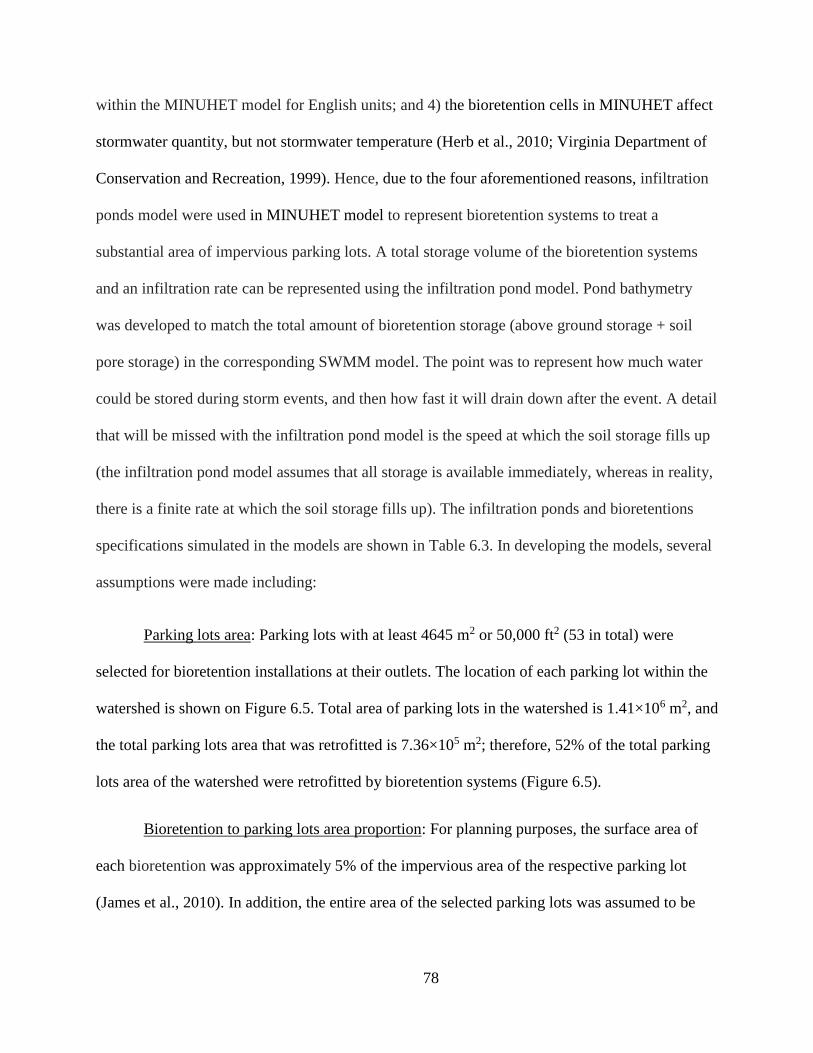
78
within the MINUHET model for English units; and 4) the bioretention cells in MINUHET affect
stormwater quantity, but not stormwater temperature (Herb et al., 2010; Virginia Department of
Conservation and Recreation, 1999). Hence, due to the four aforementioned reasons, infiltration
ponds model were used in MINUHET model to represent bioretention systems to treat a
substantial area of impervious parking lots. A total storage volume of the bioretention systems
and an infiltration rate can be represented using the infiltration pond model. Pond bathymetry
was developed to match the total amount of bioretention storage (above ground storage + soil
pore storage) in the corresponding SWMM model. The point was to represent how much water
could be stored during storm events, and then how fast it will drain down after the event. A detail
that will be missed with the infiltration pond model is the speed at which the soil storage fills up
(the infiltration pond model assumes that all storage is available immediately, whereas in reality,
there is a finite rate at which the soil storage fills up). The infiltration ponds and bioretentions
specifications simulated in the models are shown in Table 6.3. In developing the models, several
assumptions were made including:
Parking lots area: Parking lots with at least 4645 m2 or 50,000 ft2 (53 in total) were
selected for bioretention installations at their outlets. The location of each parking lot within the
watershed is shown on Figure 6.5. Total area of parking lots in the watershed is 1.41×10⁶ m2, and
the total parking lots area that was retrofitted is 7.36×10⁵ m2; therefore, 52% of the total parking
lots area of the watershed were retrofitted by bioretention systems (Figure 6.5).
Bioretention to parking lots area proportion: For planning purposes, the surface area of
each bioretention was approximately 5% of the impervious area of the respective parking lot
(James et al., 2010). In addition, the entire area of the selected parking lots was assumed to be

79
treated by bioretention systems, and the overflow from the bioretention drained to the outlet of
the subwatershed.
Width vs. length dimensions: Each bioretention systems dimensions was at least assumed
to be of the ratio 1:2 (width vs. length) (James et al., 2010). For the current study, the width of
each bioretention system was assumed 6.1 m (20 ft.).
Each bioretention unit area: A number of bioretention cell units were installed at the
outlet of each selected parking lot to capture the surface runoff during storm events.
Determination the number of units of each bioretention systems was based on the area of the
respective parking lots in acres. In other words, one acre of each parking lots was assigned to one
bioretention unit. For example, if there is a 20,000 m2-parking lot (and 20,000 m2 is
approximately equivalent to 5.0 acres), and the total bioretention size assigned to this parking lot
is 5% of 20,000 m2 (i.e. 1000 m2), therefore, the number of bioretention units would be five with
each being 202 m2 in terms of area. Hence, the standard area of each bioretention unit was
chosen as 202 m2. Since each bioretention unit width was assumed 6.1 m, length of each
bioretention unit would be 33.1 m. The area of selected parking lots and bioretention systems,
and the number of bioretention units for each parking lot are shown on Appendix C.
Bioretention soil moisture: The soil moisture within each bioretention cell was assumed
to be dry, at the wilting point, initially (Rossman, 2009).
Media thickness: The Virginia Department of Environmental Quality specifies a
minimum media thickness of 61 cm (24 in) and storage layer depth of 30 cm (12 in), so these
were used (Table 6.3).

80
Media soil infiltration rate: this parameter was set at three engineered amount scenarios
of 4.16, 25, and 41.6 mm/hr. (Table 6.3). The aforementioned infiltration rates represent sandy
clay loam, sand, and sandy gravel conditions of media soil, respectively (Virginia Department of
Conservation and Recreation, 1999).
Installation of underdrain systems: Since Virginia Department of Environmental Quality
(DEQ) requires that all bioretention cells installed in karst areas (Blacksburg geology is karst)
should be lined with either a synthetic or clay liner, underdrain systems were included for all the
bioretention cells. Unlike SWMM, there is no built-in underdrain option for infiltration ponds in
the MINUHET model, which can be a source of errors in temperature simulation. The underdrain
page of the SWMM model requires the following input data: flow exponent (n), flow coefficient
(C), and offset height (Hd, mm). The outflow equation used for underdrain systems is as Eq. 6.1
(Rossman, 2009).
Q = C × (h-Hd)n Eq. 6.1
Where Q is outflow, mm/hr., and h is the height of stored water (mm). If the goal is to drain a
fully saturated soil media in a specific amount of time, a typical value for n (flow exponent)
would be 0.5 (which makes the drain act like an orifice). A rough estimate for C (flow
coefficient) would be as Eq. 6.2 (Rossman, 2009).
𝐶 =2×𝐷0.5
𝑇 Eq. 6.2
Where D is the depth of stored water (mm) and T is the time in hours to drain. A typical value
for T is 12 hr. Therefore, for the current study, n and offset height were chosen to be 0.5, and 0,
81
respectively; while C was calculated through the equation mentioned above for different depth of
water in the storage layer (Rossman, 2009).
Scenarios of bioretention installation: Four scenarios to evaluate the effectiveness of
bioretention cells were defined: 1) current condition of the watershed without retrofitting with
bioretention systems (baseline scenario), 2) installing bioretention systems with soil media
conductivity of 4.16 mm/hr., 3) installing bioretention systems with soil media conductivity of
25 mm/hr., and 4) installing bioretention systems with soil media conductivity of 41.6 mm/hr.
Model utilization: The calibrated SWMM and MINUHET models were used to simulate
streamflow, and temperature, respectively. Then, a Hybrid approach was employed to simulate
total heat load during the validation period, for each scenario.
Total streamflow (TSFs) and total heat load (THLs) for the bioretention installations are
shown in Table 6.4. Scenario 1 represents the current water condition (simulated through Hybrid
model), while scenarios 2, 3 and 4 represent media infiltration rates of 4.16, 25, and 41.6 mm/hr.,
respectively (Virginia Department of Conservation and Recreation, 1999). Scenario 3 resulted in
approximately 11% heat reduction compared to current conditions. Surprisingly, total streamflow
flow and consequently total heat load of scenario 4 was greater than scenario 3 (Table 6.4).
Scenario 3 (with soil-media infiltration rate of 25 mm/hr., which represents sand and sandy loam
soil type) resulted in better total heat reduction, while scenario 4 of bioretention installation
performed better in mitigating mean temperature (Table 6.4). The PTTET index indicates the
scenario 3 configuration of bioretention performed poorly in reducing thermal effects on trout
habitats (Table 6.4). This performance of bioretention in reducing of average temperature and
PTTET is similar to results from the Herb (2008) study on Vermillion River Watershed.
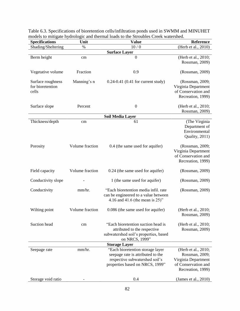
82
Table 6.3. Specifications of bioretention cells/infiltration ponds used in SWMM and MINUHET
models to mitigate hydrologic and thermal loads to the Stroubles Creek watershed. Specifications Unit Value Reference
Shading/Sheltering % 10 / 0 (Herb et al., 2010)
Surface Layer
Berm height cm 0 (Herb et al., 2010;
Rossman, 2009)
Vegetative volume Fraction 0.9 (Rossman, 2009)
Surface roughness
for bioretention
cells
Manning’s n 0.24-0.41 (0.41 for current study) (Rossman, 2009;
Virginia Department
of Conservation and
Recreation, 1999)
Surface slope Percent 0 (Herb et al., 2010;
Rossman, 2009)
Soil Media Layer
Thickness/depth cm 61 (The Virginia
Department of
Environmental
Quality, 2011)
Porosity Volume fraction 0.4 (the same used for aquifer) (Rossman, 2009;
Virginia Department
of Conservation and
Recreation, 1999)
Field capacity Volume fraction 0.24 (the same used for aquifer) (Rossman, 2009)
Conductivity slope - 1 (the same used for aquifer) (Rossman, 2009)
Conductivity mm/hr. “Each bioretention media infil. rate
can be engineered to a value between
4.16 and 41.6 (the mean is 25)”
(Rossman, 2009)
Wilting point Volume fraction 0.086 (the same used for aquifer) (Herb et al., 2010;
Rossman, 2009)
Suction head cm “Each bioretention suction head is
attributed to the respective
subwatershed soil’s properties, based
on NRCS, 1999”
(Herb et al., 2010;
Rossman, 2009)
Storage Layer
Seepage rate mm/hr. “Each bioretention storage layer
seepage rate is attributed to the
respective subwatershed soil’s
properties based on NRCS, 1999”
(Herb et al., 2010;
Rossman, 2009;
Virginia Department
of Conservation and
Recreation, 1999)
Storage void ratio - 0.4 (James et al., 2010)

83
Figure 6.5. Location and numbering of the selected parking lots within the watershed with No. 1
being the largest and No. 53 being the smallest, and a schematic example of installing
bioretention units for parking lots 1 and 13 (the green rectangular shapes represent bioretention
units).
Table 6.4. Hydrologic and thermal results of installation of bioretention systems. Scenario Total Streamflow
(m3)2
Total Heat
Load (J)3
Heat
Reduction (%)
Mean
Temperature (°C)
PTTET
(%)
11 1.95×10⁶ 1.80×10¹³ - 19.83 37.90
2 1.89×10⁶ 1.76×10¹³ -2.22 19.51 37.11
3 1.76×10⁶ 1.60×10¹³ -11.11 19.48 37.02
4 1.90×10⁶ 1.74×10¹³ -3.33 19.37 36.54
1. Represents the Current Condition or baseline scenario. 2. Simulated by SWMM model. 3. Simulated by Hybrid.

84
6.3 Canopy Thermal Effects
Vegetation and tree canopies reduce surface and air temperature through shading,
sheltering, and evapotranspiration (Bell et al., 2009). Shading and sheltering reduce solar
radiation and lower surface temperatures below canopies (which can be paved parking lots in
urbanized area). These cooler surfaces result in a reduction of heat transmitted in the local
atmosphere and building. Evapotranspiration reduces air temperature by using heat from air to
evaporate water and add moisture to the atmosphere, which results in increased humidity levels.
Various studies showed that peak air temperature in tree canopies is 5.0ºC less than open terrain
areas, and suburban surface areas with mature tree canopies are cooler than those without tree
canopies (Huang et al., 1990; Mcpherson et al., 2005; Sandifer and Givoni, 2002). This section
evaluates the effectiveness of various pervious land cover types on the reduction of heat loads
and temperatures at the watershed downstream, through the calibrated MINUHET model during
the validation period. The Stroubles Creek watershed has three main land cover types for
pervious area, which were used as input to the MINUHET model (Figure 6.6). Six scenarios of
land cover type for pervious areas (including the current condition or baseline scenario) were
designed to investigate the effects of vegetation on thermal processes within the watershed
(Table 6.5). Three land cover types of bare soil, short grass, and forest canopies were selected.
The scenarios were designed based on the current condition, minimum level, and maximum level
of vegetation density (LVD), shading for impervious land (SIL), and shading for pervious land
(SPL). The main difference between the scenarios of forest canopies (4, 5, and 6) are SIL and
SPL values, which are mainly due to the height of forest canopies for each scenario (short forest
canopies for scenario 4, and tall forest canopies for scenario 6). In addition and according to
Herb et al. (2010), the actual maximum level of shading value would be 0.9. The current

85
condition of subwatersheds LVD, SIL, and SPL are illustrated on Figure 6.6 and more
information concerning vegetation canopies of the watershed can be found on Appendix B.
Table 6.5. Various scenarios of using vegetation to reduce thermal effects in the watershed. Scenario
No.
Land cover of Watershed
Pervious Land
Vegetation
Density (%)
Shading for
Impervious Land
(%)
Shading for
Pervious Land
(%)
1 C.C.* C.C. C.C. C.C.
2 Bare Soil 0 C.C. 0
3 Short Grass 100 C.C. C.C.
4 Forest Canopies 100 C.C. C.C.
5 Forest Canopies 100 C.C. 90
6 Forest Canopies 100 90 90
* Current Condition of the watershed (referred to as the baseline scenario).
The scenarios including forest canopies resulted in lower total heat loads and average
temperatures than current conditions and short grass scenarios, primarily because of more
shading on soil and impervious surfaces, and more evapotranspiration (Figure 6.7 and Table 6.6).
Clearly, bare soil (scenario 2) resulted in higher heat loads and temperatures due to lower soil
moisture and no shading/sheltering. SIL values of the bare soil scenario are primarily due to
shading by buildings. Stream temperatures had low sensitivity to shading, while lower sensitivity
for wind sheltering; in other words, stream temperature was least impacted by wind sheltering
(approximately 0.0). SIL, such as roads with overhanging trees had the most sensitivity, since
this can drop the temperature of the pavement prior to a storm, and the temperature of the runoff
itself in the first part of a storm. Compared to impervious areas, the SPL has less of an effect,
since there is less runoff from these areas. Hence, the total heat loads of scenarios 4 and 5 are
similar in magnitude (SIL of scenario 5 was assumed equal to current conditions and SPL was
increased to 90%). In contrast, scenario 6 resulted in far less total heat load compared to scenario
4 due to increased percentage of SIL of the watershed (Figure 6.7 and Table 6.6).

86
Figure 6.6. The current dominant land cover of pervious areas of each subwatershed (based on aerial imagery and field review); the three numbers on each subwatershed represent the approximate
percentage of respective land cover type of pervious area, shading percentage of subwatershed pervious area, and shading percentage of impervious area, respectively.

87
Employing forest canopies in all pervious areas of the Stroubles Creek watershed and
assuming shading of the pervious and impervious lands of 90% yielded a 24% reduction in total
heat load from the watershed. The percentage of time temperature exceeded 21°C, which is a
threshold for trout habitats, was 33.56% for scenario 6. There was an approximately 3.5%
decrease in the aforementioned criteria compared to the baseline scenario.
Figure 6.7. Total heat load and average temperature for the vegetation scenarios.
Table 6.6. Heat load and temperature values of canopies scenarios. Scenario No. Total Heat load (J) Heat Red.* (%) Mean
Temperature (°C)
PTTET
(%)
1*** 1.40×10¹³ - 19.83 37.90
2 1.53×10¹³ 8.75 20.19 39.40
3 1.44×10¹³ 2.48 19.91 38.04
4 1.25×10¹³ -11.05 19.06 36.22
5 1.24×10¹³ -12.29 19.04 36.18
6 1.07×10¹³ -24.03 18.54 33.56
*Heat load percentage reduction compared to baseline scenario (reference temperature for heat load calculations is
17°C). The negative values represent heat load reduction while the positive values represents increased heat load;
**threshold for trout; ***Current Condition or baseline scenario.

88
6.4 A Comprehensive Plan to Mitigate Thermal Pollution
According to the simulated results concerning the effectiveness of infiltration practices
and watershed-based approaches (i.e. bioretention systems, concrete pavement/cool roofs, and
planting forests), they can be applied through a comprehensive plan to mitigate the thermal
effects of urbanization. In other words, a combination of aforementioned approaches with
optimum performance can be employed to decrease the thermal impacts of urbanization within
the Stroubles Creek watershed. Hence, the best of all scenarios of pavement/roofs installation,
bioretention practices, and vegetation canopies were employed in a single combined scenario.
The combined effects of utilizing concrete pavement and ACG roofing (scenario 9 of Table 6.1)
on the impervious lands, installing bioretention systems at the outlets of selected parking lots
(scenario 3 of Table 6.4), and planting trees in pervious areas (scenario 6 of Table 6.5), resulted
in better performance of total heat load and mean temperature reduction than any single scenario.
Total heat load reduction, mean temperature, and PTTET index of the comprehensive
plan were -69.2%, 18.02°C, and 26.61%, respectively. Using the comprehensive plan, the water
temperatures violated the temperature standard for trout approximately 13% less than the
scenario without any infiltration practices and watershed-based approaches. In other words, there
would be less (in terms of percentage of time) thermal stress on trout population.

89
Chapter 7.0 Conclusion and Future Works
SWMM and MINUHET are simulation models for routing stormwater and heat loads,
respectively, through urbanized mixed-land use watersheds. SWMM and MINUHET models
produce high-resolution time series of streamflow and heat loads, respectively, at the outlet of a
watershed. To date, MINUHET has not been evaluated for an urbanized watershed of the scale
and size of the Stroubles Creek Watershed, approximately 14.1 km2 in area. Thus, in this study
MINUHET and SWMM were used to simulate streamflows and/or thermal effects of the
Stroubles Creek Watershed to serve as a case study. Further, strength of each model (i.e.
streamflow for SWMM and temperature for MINUHET) were combined in a unique hybrid
approach to increase the accuracy of heat load simulations. The models demonstrated an ability
to effectively simulate streamflow, water temperature, and heat load.
Overall, concrete pavement and ACG roof installation performed better at reducing mean
temperature, heat load, and PTTET index than bioretention systems and forest canopies in the
Stroubles Creek watershed. The comprehensive plan of utilizing infiltration practices and
watershed-based approaches resulted in lower heat reduction and outlet mean temperature than
any single scenario concrete pavement and ACG roofing, bioretention systems, and forest
canopies.
The following recommendations are made for future applications of the current models:
Incorporating MINUHET routines in SWMM submodules: A catchment-based stream
temperature model with hourly time step resolution and capability of utilizing a broad range of
LID practices is required to evaluate temperature and heat load variations of streamflow. Since
SWMM performed better at streamflow simulation, and it has a larger number of LID
90
submodels, it is recommended that SWMM be modified to incorporate thermal modeling
capability. Hence, the mentioned method allows investigation the possible stream temperature
variations impacted due to urbanization by incorporating temperature routines for both sheet and
channel flow as well as runoff routines from MINUHET into SWMM.
Conducting uncertainty analysis to identify areas in which estimates of parameters needs
to be improved: The sensitivity analysis conducted in this study determined the key parameters
and weather variables that had a substantial impact on model simulations. Hence, any uncertainty
in these parameters has the potential to considerably affect MINUHET and SWMM simulation
results. Sensitivity analysis should be conducted with the key input parameters and weather
parameters for a couple of large storm events, to investigate the extent to which input
uncertainties may affect simulation results. The sensitivity analysis conducted in this study
would provide reasonable error limits for expected uncertainties in the models inputs.
Eventually, uncertainty analysis could produce a probability distribution for the models
simulated results to assist in risk analysis.
Assess various thermal mitigation strategies with life cycle cost to identify the most cost-
effective options: Although the effectiveness of infiltration practices and watershed-based
approaches were demonstrated in this study in a number of scenarios, there is a need to assess
their implementation and maintenance costs and balance these with benefits.
Evaluate the effects of combined land use and climate changes in an analysis of
uncertainty for temperature and heat load: The potential for increases in stream heat loads and
temperature across the Stroubles Creek Watershed as a result of combined land use and climate
changes can cause challenges for the survival of sensitive aquatic species. Simulated changes to

91
the thermal and hydrologic regime of Stroubles Creek can be evaluated in response to a variety
of scenarios of projected changing climate and land use, and consider implications of thermal
stresses to sensitive aquatic species such as Trout.
Application of the models in a smaller watershed: Application of MINUHET, SWMM,
and Hybrid models in a smaller watershed would likely result in a more accurate output of
streamflow, heat load, and temperature. This is due to more accurate delineation of
pavement/roof, and vegetation canopies areas. A smaller watershed within the main Stroubles
Creek watershed could be selected, and portable gauging stations and temperature measurements
conducted at its outlet. Corresponding MINUHET, SWMM and Hybrid models could then be
developed, calibrated and validated. Infiltration practices and watershed-based thermal reduction
approaches can be assessed at a smaller scale.

92
Literature Cited
Abiy, A.Z., Demissie, S.S., MacAlister, C., Dessu, S.B., Melesse, A.M., 2016. Groundwater
Recharge and Contribution to the Tana Sub-basin, Upper Blue Nile Basin, Ethiopia, in:
Landscape Dynamics, Soils and Hydrological Processes in Varied Climates. pp. 463–481.
doi:10.1007/978-3-319-18787-7_22
Agersborg, H.P.K., 1930. The Influence of Temperature on Fish. Ecology 11, 136–144.
doi:10.2307/1930786
Ahmadisharaf, E., Tajrishy, M., Alamdari, N., 2016. Integrating flood hazard into site selection
of detention basins using spatial multi-criteria decision-making. J. Environ. Plan. Manag.
59, 1397–1417. doi:10.1080/09640568.2015.1077104
Al-Abed, N., Al-Sharif, M., 2008. Hydrological modeling of Zarqa River Basin - Jordan using
the hydrological simulation program - FORTRAN (HSPF) model. Water Resour. Manag.
22, 1203–1220. doi:10.1007/s11269-007-9221-9
Alamdari, N., Sample, D., Steinberg, P., Ross, A., Easton, Z., 2017. Assessing the Effects of
Climate Change on Water Quantity and Quality in an Urban Watershed Using a Calibrated
Stormwater Model. Water 2017, Vol. 9, Page 464 9, 464. doi:10.3390/W9070464
Barco, J., Wong, K.M., Stenstrom, M.K., 2008. Automatic Calibration of the U.S. EPA SWMM
Model for a Large Urban Catchment. J. Hydraul. Eng. 134, 466–474.
doi:10.1061/(ASCE)0733-9429(2008)134:4(466)
Beaufort, A., Moatar, F., Curie, F., Ducharne, A., Bustillo, V., Thiéry, D., 2016. River
Temperature Modelling by Strahler Order at the Regional Scale in the Loire River Basin,
France. River Res. Appl. 32, 597–609. doi:10.1002/rra.2888
Bell, R., Cole, D., Deangelo, B., Desaultes, L., Dickerhoff, E., Estes, M., Heisler, G., Hitchcock,
D., Klunich, K., Kollin, C., Lewis, M., Magee, J., Mcpherson, G., Nowak, D., Rodbell, P.,
Rosenthal, J., Sarkovich, M., Wolf, K., Yarbrough, J., Zalph, B., 2009. Reducing Urban
Heat Islands: Compendium of Strategies: Trees and Vegetation.
Bogan, T., 2003. Stream temperature-equilibrium temperature relationship. Water Resour. Res.
39, 1–12. doi:10.1029/2003WR002034
Caissie, D., 2006. The thermal regime of rivers: A review. Freshw. Biol. 51, 1389–1406.
doi:10.1111/j.1365-2427.2006.01597.x
Company, B.M., 2002. BERRIDGE SRI VALUES [WWW Document].
doi:http://www.berridge.com/colors/sri-values-for-berridge-cool-roof-colors/
Cooter, E.J., Cooter, W.S., 1990. Impacts of greenhouse warming on water temperature and
water quality in the southern United States. Clim. Res. 1, 1–12.

93
Dietz, M.E., Clausen, J.C., 2005. a Field Evaluation of Rain Garden Flow and Pollutant
Treatment. Water. Air. Soil Pollut. 167, 123–138.
Eckhardt, K., 2008. A comparison of baseflow indices, which were calculated with seven
different baseflow separation methods. J. Hydrol. 352, 168–173.
doi:10.1016/j.jhydrol.2008.01.005
Elliott, J.M., Elliott, J.A., 1995. The effect of the rate of temperature increase on the critical
thermal maximum for parr of Atlantic salmon and brown trout. J. Fish Biol. 47, 917–919.
doi:10.1111/j.1095-8649.1995.tb06014.x
Evans, E.C., McGregor, G.R., Petts, G.E., 1998. River energy budgets with special reference to
river bed processes. Hydrol. Process. 12, 575–595. doi:10.1002/(SICI)1099-
1085(19980330)12:4<575::AID-HYP595>3.0.CO;2-Y
Ferguson, B., Fisher, K., Golden, J., Hair, L., Haselbach, L., Hitchcock, D., Kaloush, K.,
Pomerantz, M., Tran, N., Waye, D., 2008. Reducing Urban Heat Islands: Compendium of
Strategies, Cool Pavements.
Gorney, R.M., Williams, M.G., Ferris, D.R., Lance, R., Gorney, R.M., Williams, M.G., 2012.
The University of Notre Dame The Influence of Channelization on Fish Communities in an
Agricultural Coldwater Stream System Source : The American Midland Naturalist , Vol .
168 , No . 1 ( July 2012 ), pp . 132-143 Published by : The University of Notre Da.
Green, W.H., Ampt, G., 1911. Studies on soil physics: I. Flow of air and water throught soils. J.
Agric. Sci. 4, 1–24.
Gupta, Vijai, H., Sorooshian, S., Yapo, Ogou, P., 1999. Status of Automatic Calibration for
Hydrologic Models: Comparison with Multilevel Expert Calibration. J. Hydrol. Eng. 4,
135–143.
Herb, W.R., 2008. Analysis of the effect of stormwater runoff volume regulations on thermal
loading to the Vermillion River. St. Anthony Falls Lab. Proj. Reports 1–34.
Herb, W.R., Janke, B., Mohseni, O., Stefan, H.G., 2010. MINUHET (Minnesota Urban Heat
Export Tool) USER MANUAL.
Herb, Erickson, T., Stefan, H.G., 2009a. Stream Temperature Modeling of Miller Creek , Duluth
, Minnesota by, ST. ANTHONY FALLS LABORATORY Engineering, Minnesota
Pollution Control Agency.
Herb, Janke, B., Mohseni, O., Stefan, H.G., 2009b. Runoff Temperature Model for Paved
Surfaces. J. Hydrol. Eng. 14, 1146–1155. doi:10.1061/(ASCE)HE.1943-5584.0000108
Herb, Mohseni, O., Stefan, H.G., 2009c. Simulation of temperature mitigation by a stormwater
detention pond. J. Am. Water Resour. Assoc. 45, 1164–1178. doi:10.1111/j.1752-
1688.2009.00354.x
94
Hester, E.T., Bauman, K.S., 2013. Stream and Retention Pond Thermal Response to Heated
Summer Runoff From Urban Impervious Surfaces. J. Am. Water Resour. Assoc. 49, 328–
342. doi:10.1111/jawr.12019
Hester, E.T., Doyle, M.W., 2011. Human impacts to river temperature and their effects on
biological processes: A quantitative synthesis. J. Am. Water Resour. Assoc. 47, 571–587.
doi:10.1111/j.1752-1688.2011.00525.x
Hofmeister, K.L., Cianfrani, C.M., Hession, W.C., 2015. Complexities in the stream temperature
regime of a small mixed-use watershed, Blacksburg, VA. Ecol. Eng. 78, 101–111.
doi:10.1016/j.ecoleng.2014.05.019
Huang, Y.J., Akbari, H., Taha, H., 1990. The wind-shielding and shading effects of trees on
residential heating and cooling requirements, in: Proceedings of the ASHRAE Winter
Conference. United States, pp. 11–14.
Huber, W.C., Dickinson, R.E., 1988. Storm Water Management Model , Version 4 : User’s
Manual 720. doi:EPA/600/3-88/001a
Iowa storm water management manual, 2008. Iowa storm water management manual.
James, L., Burges, S., 1982. Selection, calibration, and testing of hydrologic models. Hydrol.
Model. small watersheds.
James, W., Rossman, L.A., James, W.R.., 2010. User’s guide to SWMM5.
Janke, B.D., Herb, ; William R., Mohseni, ; Omid, G., S. and H., 2013. Case Study of Simulation
of Heat Export by Rainfall Runoff from a Small Urban Watershed Using MINUHET. J.
Hydrol. Eng. 18, 995–1006.
Janke, B.D., Herb, W.R., Mohseni, O., Stefan, H.G., 2009. Simulation of heat export by rainfall-
runoff from a paved surface. J. Hydrol. 365, 195–212. doi:10.1016/j.jhydrol.2008.11.019
Johnson, S., 2004. Factors influencing stream temperatures in small streams: substrate effects
and a shading experiment. Can. J. Fish. Aquat. Sci. 61, 913.
Jones, M., Hunt, W., 2009. Bioretention impact on runoff temperature in trout sensitive waters. J.
Environ. Eng. 577–585. doi:10.1061/41009(333)80
Jones, M.P., Hunt, W.F., 2010. Effect of Storm-Water Wetlands and Wet Ponds on Runoff
Temperature in Trout Sensitive Waters. J. Irrig. Drain. Eng. 136, 656–661.
doi:doi:10.1061/(ASCE)IR.1943-4774.0000227
Jones, M.P., Hunt, W.F., Winston, R.J., 2012. Effect of Urban Catchment Composition on
Runoff Temperature. J. Environ. Eng. 138, 1231–1236. doi:doi:10.1061/(ASCE)EE.1943-
7870.0000577
Kavianipour, A., Beck, J. V., 1977. Thermal property estimation utilizing the Laplace transform

95
with application to asphaltic pavement. Int. J. Heat Mass Transf. 20, 259–267.
doi:10.1016/0017-9310(77)90212-5
Ketabchy, M., Nayeb Yazdi, M., Ahamdisharaf, E., 2016a. An Overview on Geographic
Information System ( GIS ) Application in Environmental Management , Case Study :
Algae Growth Assessment in Tampa Bay. Casp. Sea J. 10, 8–13.
Ketabchy, M., Tajrishy, M., Ahmadisharaf, E., 2016b. Development of Permeable Pavement
Design Model (PPDM) for Runoff Reduction and Pollutant Removal Efficiency Prediction,
in: EWRI Congress Annual Meeting Abstract. West Palm Beach, FL.
doi:http://eventscribe.com/2016/ASCE-EWRI/ajaxcalls/presentationinfo.asp?pres=140280
Kinouchi, T., Yagi, H., Miyamoto, M., 2007. Increase in stream temperature related to
anthropogenic heat input from urban wastewater. J. Hydrol. 335, 78–88.
doi:10.1016/j.jhydrol.2006.11.002
Kong, F., Ban, Y., Yin, H., James, P., Dronova, I., 2017. Modeling stormwater management at
the city district level in response to changes in land use and low impact development.
Environ. Model. Softw. 95, 132–142. doi:http://dx.doi.org/10.1016/j.envsoft.2017.06.021
Li, H., Harvey, J.T., Holland, T.J., Kayhanian, M., 2013. Corrigendum: The use of reflective and
permeable pavements as a potential practice for heat island mitigation and stormwater
management. Environ. Res. Lett. 8, 49501. doi:10.1088/1748-9326/8/4/049501
Long, D.L., Dymond, R.L., 2014. Thermal Pollution Mitigation in Cold Water Stream
Watersheds Using Bioretention. J. Am. Water Resour. Assoc. 50, 977–987.
doi:10.1111/jawr.12152
Lott, D.A., Stewart, M.T., 2016. Base flow separation: A comparison of analytical and mass
balance methods. J. Hydrol. 535, 525–533. doi:10.1016/j.jhydrol.2016.01.063
Luca, J., Mrawira, D., 2005. New Measurement of Thermal Properties of Superpave Asphalt
Concrete. J. Mater. Civ. Eng. ASCE 17, 72–79. doi:10.1061/(ASCE)0899-1561(2005)17
Mcpherson, G., Simpson, J.R., Peper, P.J., Maco, S.E., Xiao, Q., 2005. Municipal Forest
Benefits and Costs in Five US Cities. J. For.
Mohegh, A., Rosado, P., Jin, L., Millstein, D., Levinson, R., Ban-Weiss, G., 2017. Modeling the
climate impacts of deploying solar reflective cool pavements in California cities. J.
Geophys. Res. Atmos. 122, 6798–6817. doi:10.1002/2017JD026845
Moore, W., Mirshahi, M., Bates, K., Thrasher, B., 2016. 2016 Road and Bridge Specifications.
doi:http://www.virginiadot.org/business/resources/const/VDOT_2016_RB_Specs.pdf
Moriasi, D.N., Arnold, J.G., Van Liew, M.W., Binger, R.L., Harmel, R.D., Veith, T.L., 2007.
Model evaluation guidelines for systematic quantification of accuracy in watershed
simulations. Trans. ASABE 50, 885–900. doi:10.13031/2013.23153

96
Morrill, J.C., Bales, R.C., Conklin, M.H., 2005. Estimating stream temperature from air
temperature: Implications for future water quality. J. Environ. Eng. 131, 139–146.
doi:10.1061/(asce)0733-9372(2005)131:1(139)
Mostaghimi, S., Benham, B., Brannan, K., Dillaha, T.A., Wagner, R., Wynn, J., Y., G.,
Zeckoski, R., 2003. Benthic TMDL for Stroubles Creek in Montgomery County, Virginia.
Nash, J.E., Sutcliffe, J. V, 1970. River Flow Forecasting Through Conceptual Models Part I-a
Discussion of Principles*. J. Hydrol. 10, 282–290. doi:10.1016/0022-1694(70)90255-6
Nayeb Yazdi, M., Delavarrafiee, M., Arhami, M., 2015. Evaluating near highway air pollutant
levels and estimating emission factors: Case study of Tehran, Iran. Sci. Total Environ.
doi:10.1016/j.scitotenv.2015.07.141
Neff, B.P., Day, S.M., Piggott, A.R., Fuller, L.M., 2005. Base flow in the Great Lakes basin.
U.S. Geol. Surv. Sci. Investig. Rep. 32.
NRCS, 2007. National Engineering Handbook Chapter 7 Hydrologic Soil Groups, United States
Department of Agriculture.
doi:https://directives.sc.egov.usda.gov/OpenNonWebContent.aspx?content=17757.wba
NRCS, 1986. Urban Hydrology for Small Watersheds TR-55. USDA Nat. Resour. Conserv.
Serv. Conserv. Engeneering Div. Tech. Release 55 164. doi:Technical Release 55
Rawls, W.J., 2006. Infiltration properties, 2nd Ed. ed. Taylor and Francis, Boca Raton, FL.
Rossman, L.A., 2009. Storm Water Management Model: User’s Manual.
doi:https://www.epa.gov/water-research/storm-water-management-model-swmm
Sandifer, S., Givoni, B., 2002. THERMAL EFFECTS OF VINES ON WALL
TEMPERATURES-COMPARING LABORATORY AND FIELD COLLECTED DATA,
in: Proceedings of the Annual Conference of the American Solar Energy Society. Reno,
NV.
Selbig, W.R., 2015. Simulating the effect of climate change on stream temperature in the Trout
Lake Watershed, Wisconsin. Sci. Total Environ. 521–522, 11–18.
doi:10.1016/j.scitotenv.2015.03.072
Singh, J., Knapp, H.V., Arnold, J.G., Demissie, M., 2004. Hydrologic Modeling of the Iroquois
River Watershed Using HSPF and SWAT. J. Am. Water Resour. Assoc. 41, 343–360.
doi:10.1111/j.1752-1688.2005.tb03740.x
Stefan, H.G., Herb, W.R., Janke, B., Mohseni, O., Stefan, H.G., 2008. Thermal Pollution of
Streams by Runoff From Paved Surfaces. Hydrol. Process. 22, 987–999.
doi:10.1002/hyp.6986
Taylor, C.A., Stefan, H.G., 2009. Shallow groundwater temperature response to climate change
and urbanization. J. Hydrol. 375, 601–612. doi:10.1016/j.jhydrol.2009.07.009
97
The Virginia Department of Environmental Quality, 2011. VA DEQ STORMWATER DESIGN
SPECIFICATION NO. 9 BIORETENTION.
doi:http://www.vwrrc.vt.edu/swc/documents/2013/DEQ%20BMP%20Spec%20No%209_B
IORETENTION_FinalDraft_v1-9_03012011.pdf
Thompson, A.M., Kim, K., Vandermuss, A.J., 2008. Thermal characteristics of stormwater
runoff from asphalt and sod surfaces. J. Am. Water Resour. Assoc. 44, 1325–1336.
doi:10.1111/j.1752-1688.2008.00226.x
Virginia Department of Conservation and Recreation, 1999. Virginia Stormwater Management
Handbook Volume I I, 619.
Wakchaure, A.S., Randolph, J., Zahm, D., Carstensen, L.W., 2001. An ArcView tool for
simulating Land Subdivision for Build Out Analysis. Virginia Tech.
doi:https://vtechworks.lib.vt.edu/bitstream/handle/10919/37156/Ashwini_W_Project.pdf?se
quence=1
Walsh, C.J., Allison, H.R., Feminella, J.W., Cottingham, P.D., Groffman, P.M., Ii, R.P.M., 2005.
The urban stream syndrome: current knowledge and the search for a cure. J. North Am.
Benthol. Soc. 24, 706–723. doi:10.1899/04-028.1
Wanielista MP, 1997. Hydrology and water quality control, 2nd edn. ed. Wiley, New York.
Webb, B., Zhang, Y., 1999. Water temperatures and heat budgets in Dorset chalk water courses.
Hydrol. Process. 13, 309–321. doi:10.1002/(sici)1099-1085(19990228)13:3<309::aid-
hyp740>3.0.co;2-7
Wehrly, Wang, L., Mitro, M., 2007. Field-Based Estimates of Thermal Tolerance Limits for
Trout: Incorporating Exposure Time and Temperature Fluctuation. Trans. Am. Fish. Soc.
136, 365–374. doi:10.1577/T06-163.1
Xin, Z., Kinouchi, T., 2013. Analysis of stream temperature and heat budget in an urban river
under strong anthropogenic influences. J. Hydrol. 489, 16–25.
Xing, W., Li, P., Cao, S., Gan, L., Liu, F., Zuo, J., 2016. Layout effects and optimization of
runoff storage and filtration facilities based on SWMM simulation in a demonstration area.
Water Sci. Eng. 9, 115–124. doi:http://dx.doi.org/10.1016/j.wse.2016.06.007

98
Appendix A. The geologic map of the Stroubles Creek Watershed
The geologic map of the Stroubles Creek Watershed (georeferenced and digitized as a
hard copy from the Geology and Mineral Resources Division of Commonwealth of Virginia,
1985) is displayed in Figure A.1 (https://www.dmme.virginia.gov/dgmr/mapspubs.shtml). Below
are the descriptions regarding the geologic characteristics of areas of the watershed; the
followings description can be used as legend for Figure A.1.
Al (Alluvium; the area along the Stroubles Creek, which is represented by red yellow
color): Floodplain deposits of stratified light-gray to light-brown, unconsolidated sand, silt, and
clay with beds and lenses of pebbles and cobbles. Thickness: 0-9.2m.
Td (Talus deposits; the area beneath the ponds of the watershed, which is represented by
yellow): Unconsolidated, unsorted boulder fields composed of 0.3-1.8m thick angular boulders
of quartzite, siliceous sandstone and quartzes conglomerate. This detritus has been derived from
nearby state of Mississippian, Silurian and Devonian age. Thickness: 0-9.2m.
Ce (Elbrook Formation; which is represented by red color): The uppermost part of the
formation is characterized by interbedded sandy, commonly crossbed, fine-grain dolomite
containing thin (1-10cm) lenses of fine to medium-grained sandstone and 0.3-1.2m thick ribbon-
banded limestone dolomite.
Cr (Rome Formation; the area mostly at the eastern portion of the watershed, which is
represented by red color and black lines): Consists of interbedded mottled, maroon and green
phylittic mudstone, fine-grained sandstone and siltstone, and dark-gray, fine-grained dolomite.

99
Ccr (Copper Ridge Formation; the area upstream of the watershed, which is represented
by yellow color): inter-bedded medium-gray, fine to medium-grained locally grained, massive
dolomite, supper siliceous oolite and quartzose sandstone. Total thickness is about 366m.
Figure A.1. The geologic map of the Stroubles Creek Watershed.

100
Appendix B. Watershed Characteristics as Input to the SWMM Model
The subwatershed characteristics, which were used as input to the Calibrated SWMM
Model, are shown in Figure B.1 and Table B.1. In addition to SWMM, the input data used for
subwatershed characteristics of MINUHET model are shown in Table B.2. Area, length, width,
roughness and slope parameters values used for pervious and impervious lands of SWMM model
were used as input for MINUHET model as well; hence, the parameters mentioned above are not
included in Table B.2.
Figure B.1. The subwatershed delineation; the numbers on each subwatershed represent
subwatershed No.

101
Table B.1. The input watershed parameters for the calibrated SWMM model.
Wat. No.*
Area
(m2)
Width
(m)
Slope
(%)
Imperv.
(%)
N
Imperv.*
N
Perv.*
Suction
Head
(cm)
Conductivity
(mm/hr.)
Initial
Deficit
(frac.)
2 2.14E+05 620 1.12 37 0.010 0.239 16.99 7.87 0.284
4 5.07E+04 354 1.25 37 0.012 0.342 16.99 6.15 0.284
5 2.21E+05 271 0.81 53 0.009 0.365 14.00 7.98 0.237
6 8.07E+04 213 0.94 50 0.013 0.369 16.99 7.29 0.284
7 1.95E+05 946 0.89 51 0.011 0.348 14.00 9.53 0.237
8 1.94E+05 304 1.46 26 0.011 0.355 24.00 5.84 0.284
9 6.68E+05 772 1.10 40 0.013 0.343 24.00 5.94 0.284
11 9.10E+05 733 1.40 26 0.009 0.220 24.00 4.37 0.284
12 1.04E+05 203 0.58 41 0.014 0.350 21.50 1.30 0.244
13 3.93E+04 231 0.46 55 0.010 0.231 24.00 0.81 0.321
15 2.36E+05 957 0.60 48 0.009 0.339 08.53 20.14 0.147
16 3.63E+05 583 0.98 32 0.010 0.305 14.00 10.36 0.237
17 2.12E+05 661 1.74 22 0.014 0.386 6.10 34.34 0.105
18 9.60E+05 674 0.78 50 0.008 0.245 14.00 7.32 0.237
21 4.24E+05 551 0.86 29 0.012 0.326 24.00 6.10 0.284
22 7.06E+04 512 1.18 15 0.012 0.356 09.14 11.46 0.170
23 8.18E+05 568 0.73 50 0.011 0.218 32.00 0.05 0.378
24 1.74E+05 1161 1.76 12 0.011 0.291 19.48 4.14 0.264
25 8.04E+05 930 0.85 30 0.011 0.341 24.00 6.63 0.284
26 2.72E+05 392 0.83 28 0.013 0.292 07.90 21.16 0.140
27 1.02E+06 830 0.99 35 0.012 0.329 11.00 12.80 0.190
28 7.56E+05 541 0.98 21 0.013 0.291 11.00 11.51 0.190
29 3.37E+05 403 0.96 46 0.013 0.279 14.00 5.87 0.237
30 6.92E+05 695 0.73 15 0.014 0.354 14.00 6.65 0.237
31 5.60E+05 605 0.89 24 0.012 0.280 14.00 9.58 0.237
32 1.32E+06 915 0.80 33 0.013 0.260 12.93 5.16 0.264
34 9.43E+05 732 0.78 20 0.011 0.366 14.00 11.43 0.237
35 5.93E+05 510 0.92 10 0.008 0.275 14.00 8.71 0.237
38 6.99E+04 244 1.80 7 0.009 0.291 12.93 3.25 0.264
39 1.33E+04 182 0.77 61 0.013 0.300 12.93 3.63 0.264
40 1.96E+04 294 0.85 43 0.009 0.229 10.29 10.36 0.180
41 7.82E+04 418 1.29 29 0.008 0.316 14.00 9.98 0.237
42 2.99E+04 253 1.56 38 0.010 0.262 14.00 6.93 0.237
43 6.78E+04 240 1.75 31 0.013 0.302 19.48 4.01 0.264
44 9.22E+04 222 1.50 26 0.008 0.341 11.00 15.21 0.190
45 1.07E+05 176 0.96 25 0.010 0.364 21.50 1.47 0.244
47 3.16E+04 200 0.93 44 0.012 0.344 05.97 44.73 0.090
48 9.70E+04 435 0.80 30 0.010 0.286 21.50 1.40 0.244
49 1.58E+04 72 0.77 55 0.010 0.274 14.00 7.67 0.237

102
Continuation of previous page
50 4.06E+04 110 0.98 68 0.013 0.388 14.00 7.34 0.237
51 2.61E+04 73 2.02 22 0.014 0.385 06.10 33.81 0.105
52 2.49E+05 447 1.61 29 0.012 0.366 11.00 8.92 0.190
53 2.43E+04 141 0.69 62 0.009 0.232 24.00 7.92 0.284
*Wat: Watershed; N Imperv.: Manning’s n for impervious area; N Perv.: Manning’s n for pervious area.
Table B.2. The input watershed parameters for the calibrated MINUHET model. Pervious Land Impervious Land
Wat.
No.1
Shading
(%)2
Soil
Type3
Soil moisture
status4
Vegetation
density (%)5
Dominant
Land use6
Shading
(%)
Dominant
Land use7
2 45 C nor8 90 S.G10 0 RR9
4 15 C nor 90 S.G 5 RR
5 10 B nor 100 S.G 10 RR
6 0 C nor 90 S.G 0 CR9
7 0 C nor 90 S.G 10 RR
8 25 C nor 70 S.G 10 A9
9 45 C nor 90 S.G 0 A
11 50 C nor 70 S.G 25 RR
12 35 C nor 90 S.G 10 RR
13 5 C nor 90 S.G 10 A
15 0 C nor 100 S.G 0 A
16 15 C nor 100 S.G 10 A
17 80 C nor 80 F10 20 RR
18 5 C nor 100 S.G 5 RR
21 0 C nor 90 S.G 10 A
22 10 C nor 90 R.C 5 A
23 10 C nor 90 S.G 15 CR
24 10 C nor 85 S.G 10 RR
25 0 C nor 100 S.G 10 CR
26 10 C nor 60 R.C 0 RR
27 15 C nor 100 S.G 5 A
28 0 B nor 80 R.C 5 RR
29 5 B nor 100 S.G 0 RR
30 5 B nor 80 R.C 0 CR
31 10 B nor 80 S.G 10 A
32 15 C nor 100 S.G 10 CR
34 0 B nor 80 R.C10 0 RR
35 15 B nor 80 R.C 10 RR
38 10 C nor 90 R.C 10 C9
39 10 C nor 90 S.G 0 A
40 0 C nor 100 S.G 0 A
41 10 B nor 80 S.G 10 CR
42 20 C nor 90 S.G 10 RR
43 20 C nor 90 S.G 10 RR

103
Continuation of previous page
44 15 C nor 80 S.G 10 A
45 40 C nor 100 S.G 10 RR
47 15 B nor 100 S.G 15 A
48 25 C nor 100 S.G 5 RR
49 10 C nor 90 S.G 10 RR
50 25 C nor 90 S.G 5 A
51 10 C nor 80 S.G 5 A
52 10 C nor 100 S.G 15 A
53 0 C nor 100 S.G 0 A
1. Wat: Watershed.
2. The degree of shading from trees and buildings, 0.0 = no shading, 100= full shading.
3. USDA hydrologic soil group.
4. Near surface soil moisture prior to storm events.
5. The vegetation canopy density, 0.0 = no vegetation, 100 = full vegetation.
6. The dominant pervious land use for the watershed.
7. The dominant impervious surface type.
8. Normal.
9. RR: Residential Roof, CR: Commercial Roof, A: Asphalt, C: Concrete.
10. S.G: Short Grass, F: Forest, R.C: Row_Crop

104
Appendix C. Areas of parking lots and bioretention systems, and number of bioretention
units for each parking lots
Table C.1. Areas of parking lots and bioretention systems, and number of bioretention units for
each parking lots. Parking Lot No. Parking Lot Area (m2) Total Bioretention are (m2)1 No. of Bioretention Units2
1 46016 2301 11
2 46016 2301 11
3 40491 2025 10
4 31425 1571 8
5 28706 1435 7
6 27538 1377 7
7 25693 1285 6
8 24386 1219 6
9 24353 1218 6
10 23009 1150 6
11 22952 1148 6
12 21504 1075 5
13 20837 1042 5
14 19437 972 5
15 16998 850 4
16 16334 817 4
17 14790 739 4
18 13396 670 3
19 12723 636 3
20 12108 605 3
21 11810 590 3
22 11810 590 3
23 11492 575 3
24 11271 564 3
25 10870 544 3
26 9443 472 2
27 9344 467 2
28 9344 467 2
29 9026 451 2
30 8865 443 2
31 8380 419 2
32 8036 402 2
33 7642 382 2
34 7321 366 2
35 7276 364 2
36 7167 358 2

105
Continuation of previous page
37 7159 358 2
38 6298 315 2
39 6228 311 2
40 6214 311 2
41 6119 306 2
42 6114 306 2
43 5878 294 1
44 5781 289 1
45 5677 284 1
46 5505 275 1
47 5437 272 1
48 5433 272 1
49 5429 271 1
50 5327 266 1
51 5250 263 1
52 5128 256 1
53 5038 252 1
1. It represents 5% of respective parking lot area. 2. Each bioretention unit area is assigned to 202 m2.
106
Appendix D. The baseflow separation method
Baseflow separation involves separating stream hydrograph into baseflow and runoff. The
most widely used methods of baseflow separation are analytical methods (Lott and Stewart,
2016). A hydrograph is composed of long and short waves; analytical methods assume that the
long waves are due to baseflow with a lower amplitude, while direct runoff makes shorter waves
with greater frequency variability of streamflow (Abiy et al., 2016). Eckhardt, (2008) developed
a two parameters equation through numerical analysis for baseflow separation, which is provided
in Eq. 5
𝑏𝑘 = (1−𝐵𝐹𝐼max)𝑎𝑏𝑘−1+(1−𝑎)𝐵𝐹𝐼×𝑦𝑘
1−𝑎𝐵𝐹𝐼𝑚𝑎𝑥 Eq. D.1
Where a is, the groundwater recession constant, y is the total streamflow, b is the baseflow, and
k is the time step number. There are three values for maximum baseflow index (BFImax)
parameter; 0.80 for perennial streams with porous aquifers, 0.50 for ephemeral streams with
porous aquifers, and 0.25 for perennial streams with hard rock aquifers. In the current study, a
web-based hydrograph analysis tool (WHAT) was used for baseflow separation using the
Eckhardt method (Eckhardt, 2008). The aforementioned method is able to separate baseflow
more accurate than other numerical methods, since it utilizes two-parameter filters (Eckhardt,
2008; Neff et al., 2005). Since the current stream study is perennial with porous aquifers
underneath, a BFImax of 0.80 was applied.