arX

iv:m

ath/

0110

195v

2 [

mat

h.A

P] 2

0 M

ar 2

002

Thermal convection in a cylindrical annulus heated

laterally

S. Hoyas⋆, H. Herrero⋆ and A. M. Mancho†⋆ Departamento de Matematicas, Facultad de Ciencias Quımicas

Universidad de Castilla-La Mancha, 13071 Ciudad Real, Spain.

† Department of Mathematics, School of Mathematics

University of Bristol, University Walk,

Bristol BS8 1TW, United Kingdom.

E-mail: Sergio.Hoyas@uclm.es (S Hoyas), Henar.Herrero@uclm.es

(H Herrero) and A.M.Mancho@Bristol.ac.uk (A M Mancho)

December 4, 2017

Abstract

In this paper we study thermoconvective instabilities appearing in a fluid within acylindrical annulus heated laterally. As soon as a horizontal temperature gradient

is applied a convective state appears. As the temperature gradient reaches a crit-ical value a stationary or oscillatory bifurcation may take place. The problem is

modelled with a novel method which extends the one described in [10]. The NavierStokes equations are solved in the primitive variable formulation, with appropriate

boundary conditions for pressure. This is a low order formulation which in cylin-drical coordinates introduces lower order singularities. The problem is discretized

with a Chebyshev collocation method easily implemented and its convergence has

been checked. The results obtained are not only in very good agreement with thoseobtained in experiments, but also provide a deeper insight into important physical

parameters developing the instability, which has not been reported before.

1

1 Introduction

The problem of thermoconvective instabilities in fluid layers driven by a temperature

gradient has become a classical subject in fluid mechanics [1, 2]. It is well known thattwo different effects are responsible for the onset of motion when the temperature

difference becomes larger than a certain threshold: gravity and capillary forces.When both effects are taken into account the problem is called Benard-Marangoni

(BM) convection [3].To solve numerically hydrodynamical problems in the primitive variable for-

mulation raises two questions, one is the handling of first order derivatives for pres-sure and the other is finding its boundary conditions [4, 5, 6], which are not intuitive.

In thermoconvective problems pressure usually is avoided, for instance in Refs. [7, 8]the method of potentials of velocity is used to eliminate it from the equations. This

technique raises the order of the differential equations and additional boundary con-ditions may be required. This is particularly troublesome in cylindrical coordinates

where high order derivatives cause awkward difficulties. In Ref. [9] the primitivevariables formulation is used although the use of a particular spectral method allows

the removal of pressure. In Ref. [10] the linear stability analysis of two convection

problems are solved in the primitive variables formulation and taking appropriateboundary conditions for pressure. In this article very good accuracy is obtained

both for cartesian and cylindrical coordinates. This method has been succesfullyapplied to describe experimental results in cylindrical containers [11]. In this paper

we extend this method to study a BM problem in a cylinder heated laterally.The physical set up (Fig. 1) consists of a fluid filling up a container bounded

by two concentric cylinders. The upper surface is open to the air and the fluidis heated laterally through the lateral walls which are conducting. This set up

corresponds to the experiment reported in Ref. [12], and also it is comparable tosimilar experiments in rectangular containers [13, 14]. In [15] a similar problem is

treated theoretically, however in this work rotation is considered and the gravity fieldis along the radial coordinate. In the problem we treat, as soon as a slight difference

of temperature is imposed between the lateral walls, a stationary solution appearswhich is called basic state. When the temperature of the walls is modified the basic

state can become unstable and bifurcate to different patterns, both stationary andoscillatory. When the bifurcation is stationary, the emerging pattern consists of a

3D structure of rolls whose axes are parallel to the radial coordinate (radial rolls)

and in the oscillatory case, the axes are tilted with respect the radial axis. Theseresults coincide with those obtained experimentally [12, 13, 14].

The basic state is calculated solving a set of nonlinear equations wherebythe first contribution is obtained by a linear approach. To improve the solution we

expand the corrections of the unknown fields in Chebyshev polynomials, and we

2

pose the equations at the Gauss-Lobatto collocation points [16]. The bifurcationthresholds are obtained through a generalized eigenvalue problem with the same

Chebyshev collocation method. The convergence of the method is studied by com-paring different expansions.

The organization of the article is as follows. In Sec. 2 the formulation of theproblem with the equations and boundary conditions is explained. In the third sec-

tion the basic state is calculated and the results obtained are discussed for different

physical conditions. In the fourth section the linear stability of the basic solution isperformed and instabilities are studied for different parameters. In the fifth section

conclusions are detailed.

2 Formulation of the problem

The physical set up considered is shown in Fig. 1. A horizontal fluid layer of depthd (z coordinate) is in a container bounded by two concentric cylinders of radii a and

a+δ (r coordinate). The bottom plate is rigid and the top is open to the atmosphere.The inner cylinder has a temperature Tmax whereas the outer one is at Tmin and the

environment is at T0. We define T = Tmax − T0 and Th = Tmax − Tmin, whichare the main two parameters controlling instabilities in this problem. The system

evolves according to the momentum and mass balance equations and to the energyconservation principle. In the equations governing the system ur, uφ and uz are the

components of the velocity field u of the fluid, T the temperature, p the pressure,r the radio vector and t the time are denoted. The magnitudes are expressed in

dimensionless form after rescaling in the following form: r′ = r/d, t′ = κt/d2,u′ = du/κ, p′ = d2p/ (ρ0κν) , Θ = (T − T0) /T . Here κ is the thermal diffusivity, ν

the kinematic viscosity of the liquid and ρ0 is the mean density at the environmenttemperature T0.

The governing dimensionless equations (the primes in the corresponding fields

have been dropped) are the continuity equation,

∇ · u = 0. (1)

The energy balance equation,

∂tΘ+ u · ∇Θ = ∇2Θ, (2)

The Navier-Stokes equations,

∂tu+ (u · ∇)u = Pr

(

−∇p +∇2u+Rρ

αρ0Tez

)

, (3)

3

where the operators and fields are expressed in cylindrical coordinates [5] and ezis the unit vector in the z direction. Here the Oberbeck-Bousinesq approximation

has been used. It consist of considering only in the buoyant term, the followingdensity dependence on temperature ρ = ρ0 [1− α (T − T0)], where α is the thermal

expansion coefficient. The following dimensionless numbers have been introduced:

Pr =ν

κ, R =

gαTd3

κν, (4)

where g is the gravity constant. Pr is the Prandtl number which is assumed to have

a large value and R the Rayleigh number, representative of the buoyancy effect.

2.1 Boundary conditions

We discuss now the boundary conditions (bc). The top surface is flat, which impliesthe following condition on the velocity,

uz = 0, on z = 1. (5)

The variation of the surface tension with temperature is considered: σ (T ) = σ0 −

γ (T − T0) , where σ0 is the surface tension at temperature T0, γ is the constantrate of change of surface tension with temperature (γ is positive for most current

liquids). This effect supplies the Marangoni conditions for the velocity fields whichin dimensionless form are,

∂zur +M∂rΘ = 0, ∂zuφ +M

r∂φΘ = 0, on z = 1. (6)

Here M = γTd/ (κνρ0) is the Marangoni number. In our particular problem

the Rayleigh and the Marangoni numbers are related in the same way as in theexperiments in Ref. [12] M = 9.2 · 10−8R/d2, so buoyancy effects are dominant.

The remaining boundary conditions correspond to rigid walls and are expressed asfollows,

ur = uφ = uz = 0, on z = 0, (7)

ur = uφ = uz = 0, on r = a∗, r = a∗ + δ∗, (8)

where a∗ = a/d and δ∗ = δ/d.

For temperature we consider the dimensionless form of Newton’s law for heat

exchange at the surface,∂zΘ = −BΘ, on z = 1, (9)

where B is the Biot number. At the bottom a linear profile is imposed,

Θ =(

−r

δ∗+

a

δ

)

Th

T+ 1, on z = 0, (10)

4

while in the lateral walls conducting boundary conditions are considered

Θ = 1, on r = a∗, (11)

Θ =(

−1 +a

δ

)

Th

T+ 1, on r = a∗ + δ∗. (12)

¿From this boundary conditions it is clear how not only T defining the Rayleighnumber is involved in the problem, but also Th. Due to the fact that pressure is

kept in the equations, additional boundary conditions are needed. They are obtainedby the continuity equation at z = 1 and the normal component of the momentum

equations on r = a∗, r = a∗ + δ∗ and z = 0, [10].

∇ · u = 0, on z = 1, (13)

Pr−1

(

∂ur

∂t+ ur

∂ur

∂r+

uφ

r

∂ur

∂φ+ uz

∂ur

∂z−

u2φ

r

)

=

= −∂p

∂r+∆ur −

ur

r2−

2

r2∂uφ

∂φ, on r = a∗, r = a∗ + δ∗, (14)

Pr−1

(

∂uz

∂t+ ur

∂uz

∂r+

uφ

r

∂uz

∂φ+ uz

∂uz

∂z

)

=

= −∂p

∂z+∆uz − b+RT, on z = 0, (15)

where b = d3g/(κν), and ∆ = r−1∂/∂r(r∂/∂r) + r−2∂2/∂φ2 + ∂2/∂z2.

3 Basic state

As soon as the lateral walls are at different temperatures and a horizontal tem-

perature gradient is set at the bottom, a stationary convective motion appears

in the fluid. In contrast to the classical Benard-Marangoni problem with uni-form heating, here the basic state is not conductive, but convective. In order to

calculate it, for computational convenience, the following change has been per-formed: r′ = 2r/δ∗ − 2a∗/δ∗ − 1 and z′ = 2z − 1, which transforms the domain

Ω1 = [a∗, a∗ + δ∗] × [0, 2π] × [0, 1] into Ω = [−1, 1] × [0, 2π] × [−1, 1]. After thesechanges, and since the basic state has radial symmetry (there is no dependence on

φ) the steady state equations in the infinite Prandtl number approach become (theprimes have been dropped),

A∂rp+G2ur = ∆∗ur, (16)

2∂zp + b− RΘ = ∆∗uz, (17)

Gur + A∂rur + 2∂zuz = 0, (18)

urA∂rΘ+ 2uz∂zΘ = ∆∗Θ, (19)

5

where ∆∗ = A2∂2r +GA∂r+4∂2

z , b = d3g/κν, A = 2d/δ and G (r) = 2d/(2a+δ+rδ).The boundary conditions are now as follows,

uz = 2∂zur +MA∂rT = 2∂zΘ+BΘ = 0, on z = 1, (20)

Gur + A∂rur + 2∂zuz = 0, on z = 1, (21)

ur = uz = 0,Θ = (1− r)/2, on z = −1, (22)

2∂zp+ b−RΘ = ∆∗uz, on z = −1, (23)

ur = uz = 0, Θ = 0, on r = 1, (24)

A∂rp +G2ur = ∆∗ur, on r = 1, (25)

ur = uz = 0, Θ = 1, on r = −1, (26)

A∂rp +G2ur = ∆∗ur, on r = −1. (27)

3.1 Numerical method

We have solved numerically Eqs. (16)-(19) together with the boundary conditions

(20)-(27) by a Chebyshev collocation method. This approximation is given by fourperturbation fields ur (r, z) , uz (r, z) , p (r, z) and Θ (r, z) which are expanded in a

truncated series of orthonormal Chebyshev polynomials:

ur (r, z) =N∑

n=0

M∑

m=0

anmTn (r)Tm (z) , (28)

uz (r, z) =N∑

n=0

M∑

m=0

bnmTn (r) Tm (z) , (29)

p (r, z) =N∑

n=0

M∑

m=0

cnmTn (r)Tm (z) , (30)

Θ (r, z) =N∑

n=0

M∑

m=0

dnmTn (r)Tm (z) . (31)

Expressions (28)-(31) are replaced into the equations (16)-(19) and boundary condi-

tions (20)-(26). The N+1 Gauss-Lobato points (rj = cos(π(1− j/N)), j = 0, ..., N)

in the r axis and theM+1 Gauss-Lobato points (zj = cos(π(1− j/M), j = 0, ...,M)in the z axis are calculated. The previous equations are evaluated at these points ac-

cording to the rules explained in Ref. [17], in this way 4 (N + 1) (M + 1) equationsare obtained with 4 (N + 1) (M + 1) unknowns. The system has not maximun rank

because pressure is only determined up to a constant value. Since this value is notaffecting to the other physical magnitudes, we replace the evaluation of the normal

component of the momentum equations at (rj=N = 1, zj=4 = cos(π(1−4/M))) by avalue for the pressure at this point, for instance p = 0. To solve the resulting nonlin-

ear equatins, a Newton-like iterative method is used. In a first step the nonlinearity

6

is discounted and a solution is found by solving the linear system. It is corrected bysmall perturbation fields: ur (r, z) , uz (r, z) , p (r, z) and Θ (r, z) ,

ui+1

r (r, z) = uir (r, z) + ur (r, z) , (32)

ui+1

z (r, z) = uiz (r, z) + uz (r, z) , (33)

pi+1 (r, z) = pi (r, z) + p (r, z) , (34)

Θi+1 (r, z) = Θi (r, z) + Θ (r, z) , (35)

in such way that solutions at i + 1 step are obtained after solving Eqs. (16)-(26)linearized around the approach at step i. The considered criterion of convergence

is that the difference between two consecutive approximations in l2 norm should besmaller than 10−9.

3.2 Results on the basic state

Previous theoretical works [18, 19, 20] dealing with this problem have approached

the basic state solution as a parallel flow, where only the horizontal componentof the velocity field exists. This approach requires the imposition of a constant

temperature gradient over all the fluid layer and at the top boundary. In thosedescriptions this gradient becomes the main control parameter. In our model lateral

effects are considered, so parallel flow is no longer valid and no restrictions areneeded in the temperature boundary conditions which, as explained in the previous

section, is the usual Newton law. This boundary condition is the origin of twocontrol parameters related to temperature, i. e., Th and T . This possibility,

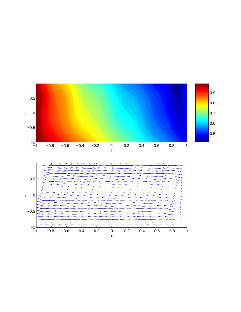
which had been already addressed in [21], is explored in detail in the next section.We have found two types of basic states. The first one, displayed in Fig. 2

shows the isotherms obtained at B = 1.25, δ∗ = 10 and ∆hT = T = 6.4oC. Thebottom profile is linear, as expected from the boundary condition, however at the

top it approaches the constant ambient temperature, since the Biot number is large.This field is similar to that of the layer heated from below, i.e. roughly speaking

hotter at the bottom. This feature is shared with the linear flow described in [20].

Fig. 3 shows the velocity fields for the same conditions. They are formed by two co-rotative rolls perpendicular to the gradient. This result is similar to that obtained

in experiments reported in Refs. [12, 13, 14], where co-rotative rolls perpendicularto the gradient are found as well. These results coincide with those obtained in Ref.

[21] for a rectangular geometry.The second kind of basic state is represented in Fig. 4 for B = 0.8, δ∗ = 2.5,

∆hT = 0.3oC, T = 1.84oC. The most striking feature is that along the verticalaxis there are changes in the sign of the temperature gradient. It seems that the

Biot number is not dissipating heat effectively at the top and then heat is advected

7

by the velocity field. This temperature profile coincides with that of the return flow

defined in Ref. [20], where the role of the transport of heat by the velocity field

as the origin of the instability is discussed. As we will demonstrate in the nextsection this flow becomes unstable through an oscillatory bifurcation, as it is also

reported in [20]. Crucial to the appearence of the two different flows described inthis section, is not only the Biot number that dissipates heat at the top, but also

the role of parameters T and Th which introduces heat into the system.

Fig. 5 shows a transition between the two states we have just described. Itis obtained at B = 0.3, δ∗ = 10, ∆hT = 10oC, T = 20.41oC. At this stage the

flow already becomes unstable through an oscillatory bifurcation.

4 Linear stability of the basic state

The stability of the basic state is studied by perturbing it with a vector field de-

pending on the r, φ and z coordinates, in a fully 3D analysis:

ur (r, φ, z) = ubr (r, z) + ur (r, z) e

imφ+λt, (36)

uφ (r, φ, z) = ubφ (r, z) + uφ (r, z) e

imφ+λt, (37)

uz (r, φ, z) = ubz (r, z) + uz (r, z) e

imφ+λt, (38)

Θ (r, φ, z) = Θb (r, z) + Θ (r, z) eimφ+λt, (39)

p (r, φ, z) = pb (r, z) + p (r, z) eimφ+λt. (40)

Here the superscript b indicates the corresponding quantity in the basic state andthe bar refers to the perturbation. We have considered Fourier modes expansions

in the angular direction, because along it the boundary conditions are periodic. Wereplace the expressions (36)-(40) into the basic equations and after linearizing the

resulting system, we obtain the following eigenvalue problem (the bars have beendropped):

∆mur − A∂rp−G2ur − 2G2imuφ = 0, (41)

∆muφ −Gimp+ 2G2imur −G2uφ = 0, (42)

∆muz − 2∂zp+RΘ = 0, (43)

Gur + A∂rur +Gimuφ + 2∂zuz = 0, (44)

∆mΘ− urA∂rΘb − ub

rA∂Θ− 2ubz∂zΘ− 2uz∂zΘ

b = λΘ, (45)

where ∆m = A2∂2r + GA∂r − m2G2 + 4∂2

z . The following boundary conditions forthe pertubations are obtained,

uz = 2∂zur +MA∂rΘ = 2∂zuφ +GMimΘ = 2∂zΘ+BΘ = 0, on z = 1,(46)

8

ur = uφ = uz = Θ = 0, on z = −1, (47)

ur = uφ = uz = 0, Θ = 0, on r = 1, (48)

ur = uφ = uz =, Θ = 0, on r = −1, (49)

together with

∆mur −A∂rp− 2G2imuφ = 0, on r = ±1, (50)

∆muz − 2∂zp+RΘ = 0, on z = −1, (51)

Gur + A∂rur +Gimuφ + 2∂zuz = 0, on z = 1. (52)

4.1 Numerical method

The eigenvalue problem is discretized with the Chebyshev collocation method usedfor the basic state. Now there is a new field, the angular velocity, which is expanded

as follows,

uφ(r, z) =N∑

n=0

M∑

m=0

enmTn (r)Tm (z) . (53)

In order to calculate the eigenfunctions and thresholds of the generalized eigenvalueproblem the equations are posed at the collocation points according to the rules

explained in [17], so that a total of 5(N+1)(M+1) algebraic equations are obtainedwith the same number of unknowns. If the coefficients of the unknowns which

form the matrices A and B satisfy det(A − λB) = 0, a nontrivial solution of the

linear homogeneous system exists. This condition generates a dispersion relationλ ≡ λ(m, R,M,B, ub,Θb, pb), equivalent to calculate directly the eigenvalues from

the system AX = λBX , where X is the vector which contains the unknowns. IfRe(λ) < 0 the basic state is stable while if Re(λ) > 0 the basic state becomes

unstable. In the Appendix a study of the convergence of the thresholds calculatedwith this method is shown.

4.2 Results on the stability analysis

The basic solutions obtained in section 3, become unstable when the control pa-rameter, T in this work, is increased. When T is changed, Th which is not

the control parameter in our choice, is fixed to a non zero value. In the exploredparameter range two types of bifurcations take place: stationary and oscillatory.

Figure 6 depicts the m dependence of Re(λ) for B = 1.25, δ∗ = 10 and Th = T

at the threshold (Tc = 6.4oC) and below it (T < 6.4oC). The bifurcation isstationary since the imaginary part of the eigenvalue λ is zero at the critical value

mc = 20. Figure 7 is similar to Figure 6 but at B = 0.5, δ∗ = 10 and Th = 5oC

9

and Tc = 8.63oC. Now the bifurcation is oscillatory since the imaginary part ofthe eigenvalue is non zero at the critical value mc = 18. In order to understand how

physical conditions affect the instability, Fig. 8 summarizes the influence of heatrelated parameters in the bifurcation. There, it is shown the critical value of Tc,

as a function of the Biot number B, for several values of Th. In this figure station-ary and oscillatory bifurcations are observed and it shows that having one or other

transition depends on an equilibrium between these parameters. Travelling waves

are favoured by systems storing a lot of heat, i.e., low values of the Biot number, andhigh values of hT , which facilitates the transport of heat by the velocity field [20].

We notice here the novelty of these results, where transitions between stationaryrolls and oscillatory waves are due to changes in heat related parameters. This has

not been reported in any experimental or theoretical work before, where transitionshave been found due to variations in Prandtl number [20] or in aspect ratio [13, 14].

In Fig. 8 it is also clear that thresholds decrease as B increases while thedependence of thresholds on Th is not monotonous, it presents a minimum for

Th = 2oC as figure 9 a) displays. In Fig. 9 b) it is shown how the criticalwavenumber increases with Th, on the other hand it remains almost constant with

B.The geometry and size of the box is also affecting the instability as it is

noticed mainly in low aspect ratio systems. Although a detailed study of patternsin small containers is beyond the scope of this work, table I gives an insight into

it. It shows the critical value of Tc and the corresponding critical wavenumber mc

for some δ∗. The wavenumber does not change monotonously with the aspect ratio,as also happens in small containers with uniform heating from below [9, 10, 11] as

well.The critical wavenumber for the stationary bifurcation shows that a 3D struc-

ture appears which consists of radial rolls whose axes are parallel to the radial co-ordinate as Fig. 10 shows for B = 1.25 and δ∗ = 10 and Tc = 6.4oC. The growing

perturbation along the transverse plane is plotted in Fig. 11, where a structureappears near the hot side as in the experiment reported in [23]. This is so because,

in this case, the instability has the same origin as a static fluid heated from below,so since the vertical temperature gradient is greater at this boundary, perturbation

grows there first. On the other hand since the hot cylinder counteracts the verticaltemperature gradient it inhibits the instability threshold. These results are in good

agreement with those obtained in Ref. [21] in similar conditions but in a cartesiangeometry. In that article at a threshold Tc = 6.8oC, the critical wavenumber is

kc = 2.4, which would correspond to 12 − 36 periods respectively in the inner and

outer radii of an annulus as ours. This matches rather well with our critical thresh-old and wavenumber which is mc = 20, suggesting that, at least for this aspect

ratio, geometry does not strongly affect the results. These results and discussions

10

of the stationary bifurcation are in good agreement with those reported in Refs.[13, 18, 19, 20, 22].

We also obtain oscillatory bifurcations. For instance, there is one at δ∗ = 10(d = 2 mm), Th = 5oC, B = 0.5 and Tc = 8.63oC, which corresponds to

travelling waves or hydrothermal waves described in Refs. [13, 12, 14]. Fig. 12depicts the eigenfunction along the transverse plane, where the tilted axis of the

waves can be seen. This result is comparable to that reported in Ref. [14] where

for a cartesian container with Lx = 20 mm, d ∼ 2 mm, hydrothermal waves ofwavenumber kc ∼ 1, emerge above a threshold. This would correspond to a pattern

with 6 − 19 periods in the inner and outer radii of our annulus respectively, whichis not far from our critical wavenumber mc = 18. The angle of inclination of the

waves in Fig. 10 is φ ∼ 3π/4 also close to that of 2.60− 1.75 rad of Ref. [14].

5 Conclusions

We have studied a BM lateral heating problem in a cylindrical annulus. The problemhas been solved with a Chebyshev collocation method by keeping the original Navier-

Stokes equations, where appropriate boundary conditions are required for pressure[10]. The scheme developed in Ref. [10] for stability problems has been extended

to calculate a non trivial basic state. The procedure is confirmed to be reliable,effective and easy to implement.

We have obtained two kinds of basic solutions. One type is formed by co-rotative rolls such as those reported in experiments [12, 13, 14], and in similar

theoretical studies [21]. The second kind of solution has similar features to those of

the return flow described in [20].The linear stability analysis of these solutions shows stationary bifurcations

to radial rolls and oscillatory bifurcations to hydrothermal waves, whose appearancehas been proved to depend on their heat related parameters (B, Th andT ). This

fact has not been adressed before, perhaps because experimentally these parame-ters are hard to manipulate. Properties of the growing patterns coincide with those

reported in previous works. Stationary solutions appear in basic flows with temper-ature profiles close to the static fluid heated from below [21, 20]. Their wavenumbers

are in the range of experimental [12, 13, 14] and theoretical studies [21]. Also thestructure in the z − r plane agrees with previous results [21, 23]. Oscillatory solu-

tions emerge from a basic state of the type of return flow as predicted in [20]. Theirstructure is comparable to that obtained in experiments [14].

Acknowledgments

We gratefully thank Christine Cantell, Maureen Mullins and Angel Garci-

martın for useful comments and suggestions. This work was partially supported by

11

a Research Grant MCYT (Spanish Government) BFM2000-0521 and by the Univer-sity of Castilla-La Mancha.

References

[1] Benard H 1900 Rev. Gen. Sci. Pures Appl. 11 1261

[2] Pearson J R A 1958 J. Fluid Mech. 4 489

[3] Nield D A 1964 J. Fluid Mech. 19 341.

[4] Gresho P M and Sani R L 1987 Int. J. Num. Meth. Fluids 7 1111

[5] Pozrikidis C 1997 Introduction to theoretical and computational fluid dynamics

(Oxford: Oxford University Press)

[6] Orszag S A, Israeli M and Deville O 1986 J. Scient. Comp. 1(1) 75

[7] Mercader I, Net M and Falques A 1991 Comp. Methods Appl. Mech. and Engrg.

91 1245

[8] Marques F, Net M, Massaquer J M and Mercader I 1993 Comp. Methods Appl.

Mech. and Engrg. 110 157

[9] Dauby P C, Lebon G and Bouhy E 1997 Phys. Rev E 56 520

[10] Herrero H and Mancho A M To appear in Int. J. Numer. Methods Fluids

http://arXiv.org/abs/math.AP/0109200

[11] Ramon M L, Maza D M, Mancini H, Mancho A M and Herrero H 2001 Int.

J. of Bifurcation and Chaos 11 (11) 2779

[12] Ezersky A B, Garcimartın A, Burguete J, Mancini H L and C. Perez-GarcıaC 1993 Phys. Rev. E 47 1126

[13] Daviaud F and Vince J M 1993 Phys. Rev. E 48 4432

[14] Burguete J, Mukolobwiez N, Daviaud F, Garnier N and Chiffaudel A 2001

Phys. Fluids 13 2773

[15] Alonso M A 1999 Ph. D. Thesis (Barcelona: Universitat Politecnica de

Catalunya)

12

[16] Canuto C, Hussaini M Y, Quarteroni A and Zang T A 1988 Spectral Methods

in Fluid Dynamics (Berlin: Springer)

[17] Hoyas S, Herrero H and Mancho A M 2001 Actas del XVII CEDYA/VII CMA

[18] Mercier J F and Normand C 1996 Phys. Fluids 8 1433

[19] Parmentier P, Regnier V and Lebon G 1993 Int. J. Heat Mass Transfer 36

2417

[20] Smith M K and Davis S H 1983 J. Fluid Mech. 132 119

[21] Mancho A M and Herrero H 2000 Phys. Fluids 12 1044

[22] Gershuni G Z, Laure P, Myznikov V M, Roux B and Zhukhovitsky E M 1992

Microgravity Q 2 141

[23] De Saedeleer C, Garcimartin A, Chavepeyer G, Platten J K and Lebon G 1996

Phys. Fluids 8(3) 670

[24] Mancho A M, Herrero H and Burguete J 1997 Phys. Rev. E 56 2916

[25] Hoyas S, Herrero H and Mancho A M, in preparation

13

Appendix

Convergence of the global numerical method

To carry out a test on the convergence of the global numerical method (calculation ofthe basic state and subsequent linear stability analysis) we compare the differences

in the thresholds of the differences of temperature (T ) to different orders of expan-sions for some values of the parameters involved in the problem: δ∗ ∈ [8.26, 10.52].

In table II the thresholds for these states varying the aspect ratio are shown for fourconsecutive expansions varying the number of polynomials taken in the r (N) and

z (M) coordinates. ¿From the table it is seen that convergence is reached within arelative precision for Tc of 10

−2. If M is increased the difference between succes-

sive expansions is order 10−1 while increasing N it is order 10−2. Further increments

of the order of the expansions give thresholds values oscillating around the quotedones, so within that error, thresholds are convergent. The range of parameters has

been selected in order to reach this convergence criterium.

14

Table captions

Table I

Critical T and critical mc vs the aspect ratio δ∗. The value of the horizontal

temperature difference is Th = 0.4 and B = 1.

Table II

Critical temperature differences (C) for different values of the aspect ratio at con-secutive orders in the expansion in Chebyshev polynomials (B = 1.25).

Figure captions

Figure 1

Problem set up (a = 0.01 m, δ = 0.02 m).

Figure 2

Isotherms of the basic state corresponding to values of the parameters R = 2228, M =

51, δ∗ = 10, B = 1.25 (∆T = 6.4oC, ∆Th = 6.4oC, d = 2 mm).

Figure 3

Velocity field at same conditions of Fig. 2.

Figure 4

Isotherms and velocity field of the basic state corresponding to values of the param-

eters R = 40995, M = 59, δ∗ = 2.5, B = 0.8 (∆T = 1.84oC, ∆Th = 0.3oC, d = 8mm).

Figure 5

Isotherms and velocity field of the basic state corresponding to values of the param-eters R = 7105, M = 163, δ∗ = 10, B = 0.3 (∆T = 20.41oC, ∆Th = 10oC, d = 2

mm).

Figure 6

Maximum real part of the growth rate λ as a function of m for basic state at M = 51,

δ∗ = 10, B = 1.25. The top line stands for the threshold condition Rc = 2228 (or

Tc = 6.4oC), and its maximum determines the critical mc. The bottom line is forR < Rc. Solid lines correspond to branches with real eigenvalues while the dotted

ones stand for complex eigenvalues.

Figure 7

15

Maximum real part of the growth rate λ as a function of m for a basic state atM = 69, δ∗ = 10, B = 0.5, at the threshold condition Rc = 3004 (or Tc = 8.63oC).

The maximum determines the critical mc. The solid line correspond to a branch withreal eigenvalues while the dotted one is for complex eigenvalues.

Figure 8

Critical T vs the Biot number B for different values of Th (δ∗ = 10).

Figure 9

Critical T and mc vs Th for δ∗ = 10 and B = 0.7.

Figure 10

Isotherms of the growing perturbation in the x− y plane at a stationary bifurcation

point (T = Th = 6.4C, δ∗ = 10, B = 1.25).

Figure 11

a) Isotherms of the growing perturbation in the r−z plane at a stationary bifurcation

point (T = Th = 6.4C, δ∗ = 10, B = 1.25). b) Velocity field of the growingperturbation in the r − z plane at same conditions.

Figure 12

a) Isotherms of the eigenfunction in the x − y plane at an oscillatory bifurcation

point (Th = 5C, T = 8.63C, δ∗ = 10, B = 0.5).

Figure 13

a) Isotherms of the eigenfunction in the r − z plane at the oscillatory bifurcation

point considered in Fig. 12. b) Velocity field of the eigenfunction in the r− z planeat same conditions.

16

Table I

δ∗ Tc mc

2.5 3.91 1110/3 2.63 15 3.28 210 4.03 10

Table II

δ∗ 13× 9 13× 13 25× 13 29× 1310.52 6.8711 6.8519 6.9551 6.922910.25 6.5131 6.5224 6.6792 6.666510.00 6.2223 6.2298 6.3717 6.39389.52 5.8794 5.9490 5.9126 5.95199.09 5.8415 6.0807 5.6626 5.68688.26 5.7341 5.9204 5.6812 5.6892

17

This figure "figure1.jpg" is available in "jpg" format from:

http://arxiv.org/ps/math/0110195v2

0.2

0.4

0.6

0.8

−1 −0.8 −0.6 −0.4 −0.2 0 0.2 0.4 0.6 0.8 1−1

−0.5

0

0.5

1

r

z

This figure "figure4.gif" is available in "gif" format from:

http://arxiv.org/ps/math/0110195v2

0.5

0.6

0.7

0.8

0.9

−1 −0.8 −0.6 −0.4 −0.2 0 0.2 0.4 0.6 0.8 1−1

−0.5

0

0.5

1

r

z

−1 −0.8 −0.6 −0.4 −0.2 0 0.2 0.4 0.6 0.8 1−1

−0.5

0

0.5

1

r

z

0 5 10 15 20 25 30−4.5

−4

−3.5

−3

−2.5

−2

−1.5

−1

−0.5

0

0.5

m

max(λ)

This figure "figure7.jpg" is available in "jpg" format from:

http://arxiv.org/ps/math/0110195v2

0 0.2 0.4 0.6 0.8 1 1.20

5

10

15

20

25

30

35

40

B

∆ T

∆ Th = 2

∆ Th = 5

∆ Th = 10

1 2 3 4 5 6 7 8 9 104

6

8

10

12

14

∆ Th

∆ T

1 2 3 4 5 6 7 8 9 1010

12

14

16

18

20

22

24

∆ Th

mc

This figure "figure10.jpg" is available in "jpg" format from:

http://arxiv.org/ps/math/0110195v2

0

5

10

15

−1 −0.8 −0.6 −0.4 −0.2 0 0.2 0.4 0.6 0.8 1−1

−0.5

0

0.5

1

r

z

−1 −0.8 −0.6 −0.4 −0.2 0 0.2 0.4 0.6 0.8 1−1

−0.5

0

0.5

1

r

z

x 10−4

This figure "figure12.jpg" is available in "jpg" format from:

http://arxiv.org/ps/math/0110195v2

This figure "figure13.jpg" is available in "jpg" format from:

http://arxiv.org/ps/math/0110195v2