TransmissionThermal Analysis of an Electrical Variable

Academic year 2018-2019

Master of Science in Electromechanical Engineering

Master's dissertation submitted in order to obtain the academic degree of

Counsellor: Dr. ir. Hendrik VansompelSupervisor: Prof. dr. ir. Peter Sergeant

Student number: 01407437Willem Maertens

TransmissionThermal Analysis of an Electrical Variable

Academic year 2018-2019

Master of Science in Electromechanical Engineering

Master's dissertation submitted in order to obtain the academic degree of

Counsellor: Dr. ir. Hendrik VansompelSupervisor: Prof. dr. ir. Peter Sergeant

Student number: 01407437Willem Maertens

The author gives permission to make this master dissertation available for consultation and to

copy parts of this master dissertation for personal use. In all cases of other use, the copyright

terms have to be respected, in particular with regard to the obligation to state explicitly the

source when quoting results from this master dissertation.

May 31, 2019

Preface

This master dissertation is submitted as a completion of the academic degree of Masterof Science in Electromechanical Engineering at Ghent University. It is the conclusion of alonger period of research on the topic of thermal modelling of electrical machines, whichhas proven to be a challenging research field. Five years ago, I have decided to startthe engineering program at Ghent University because I have always had a great interestin machines and mechanics. This broad formation made it possible to tackle numerouschallenges in the fields of thermodynamics, physics and electronics. This work is not theachievement of a single person however, and it would not have been possible to completethis research without the help and guidance of my promotor and counsellor. Therefore Iwould like to thank Prof. Dr. ir. Peter Sergeant for introducing me to the topic of EVTsystems, his advice and guidance during the research period and for his flexibility withrespect to the originally intended exchange with the university of Lille. My appreciationgoes to my counsellors for this project, Dr. ir. Hendrik Vansompel, and Ir. Florian Ver-belen. Thank you for addressing my numerous questions and for sharing your knowledgeand experiences in the field of thermal modelling. Thanks to your repeated explanationsI gained valuable insights on the topic, which has increased the quality of this work. Inaddition, I would like to mention the lab technicians Tony and Vincent. Thank you foryour assistance in the lab and for machining the sensors holders. Finally, I would like tothank my mother for proofreading this text and both my parents, my girlfriend and myclosest friends for their advice and support during my studies.

Willem MaertensGhent, May 31, 2019

Thermal Analysis of an Electrical Variable Transmission

WILLEM MAERTENS

Supervisor: Prof. Dr. ir. P. Sergeant

Counsellors: Dr. ir. H. Vansompel, Ir. F. Verbelen

Faculty of Engineering Sciences Department of Electrical Energy, Metals, Mechanical Construction

and Systems

Dissertation submitted in fulfilment of the requirements for the degree of MASTER OF SCIENCE IN

ELECTROMECHANICAL ENEGINEERING OPTION ELECTRICAL POWER ENGINEERING

Academic year 2018-2019

Keywords

Electrical Variable Transmission, EVT, thermal modelling

Abstract

In this dissertation, the development of a 2D FEM thermal model of an EVT with hybrid

excitation is discussed. This thermal model fits in an overarching framework of modelling tools

which can be used in the design process of EVT systems intended for e.g. hybrid vehicle

applications. These applications require a high power and torque density. For a lot of electrical

machines however, the attainable power and torque density is limited by temperature

constraints. A thorough understanding of the thermal behaviour is necessary to safely operate

the machine in wider ranges of torque, speed and power.

The objective of this work includes a literature study of thermal modelling techniques for

electrical machines and EVT systems in particular and the application of such techniques to the

specific case of a prototype EVT. In order to validate the outcome of the obtained model,

thermal experiments are conducted on the prototype machine. These experiments are designed

to enable an experimental validation of the model parameters with the highest uncertainty.

When thermal experiments show a discrepancy between the simulated and the actual thermal

behaviour of the EVT, it is tried to reveal the underlying shortcomings in the thermal model

and to adapt the concerned parameters in a substantiated manner. The resulting thermal model

can be used to predict the thermal temperature distribution within the prototype EVT depending

on the operating point in steady state conditions as well as for a transient analysis.

Thermal Analysis of an Electrical VariableTransmission

Willem Maertens

Supervisor(s): Prof. Dr. ir. Peter Sergeant, Dr. ir. Hendrik Vansompel

Abstract— Electric motors can have high power and torque densities,which are valuable characteristics for numerous applications. In manycases however, the attainable power and torque densities are limited by tem-perature constraints. Excessive temperatures will have a negative effect onthe lifetime of different machine components and the machine efficiencyand may even lead to early failure of the electrical machine. A thoroughunderstanding of the thermal behaviour of the device may lead to a safe op-eration in broader ranges of torque speed and power for a given machine.This paper discusses the development of a 2D FEM thermal model of anEVT with hybrid excitation. This model is validated against thermal exper-iments conducted on a prototype EVT. The thermal experiments have beendesigned in such way that the obtained data could be used to tune the mostuncertain parameters in the model.

Keywords—Thermal model, EVT

I. INTRODUCTION

ELECTRICAL machines of all kinds are widespread in themodern world. They play a key role in the modern econ-

omy and are indispensable in various industries like manufac-turing and energy production. One of the advantages of electricmotors in particular is their ability to deliver the rated torqueover a wide range of rotational speed. This is one of many rea-sons why the transport industry shows interest in electric motors.In the light of current efforts that are done to reduce vehicleweight and fuel consumption, it is favourable to have a powersource that is light and compact. Electric motors can have highpower and torque densities and are promising in this aspect.

In many cases however, the attainable power and torque den-sities are limited by temperature constraints. Too high temper-atures can reduce the lifetime of vital machine components ormay even lead to an early failure of the complete machine. Thestator, rotors, housing and bearings may suffer from thermal fa-tigue and the excessive temperatures may lead to demagneti-zation of the magnets in permanent magnet electrical machines.Furthermore, the lifetime of the winding insulation will decreaseconsiderably when the machine is operated above its tempera-ture limits for longer periods of time. Moreover, the energeticefficiency of the machine will be lower at elevated temperaturesdue to increased winding resistance and reduced magnetic sus-ceptibility of the iron in the yokes.

Thermal modelling of electrical machines has proven to bea challenging research field. Due to a lack of accurate thermaldata, many machines are only operated between conservativeboundaries in order to protect machine components from exces-sive hot spot temperatures. Improved quality of thermal modelscould give the opportunity to predict critical temperatures witha higher accuracy. In this way, the power output of a certain ma-chine can be increased without shortening it’s lifetime, or morecompact designs of the machine for the same power rating be-comes possible.

This research is devoted to the development of a thermalmodel of an electrical variable transmission with hybrid exci-tation. The electromagnetic modelling and the efficiency of thisspecific machine has been extensively studied in [1], which hasresulted in a loss model of a prototype EVT with hybrid excita-tion. The main heat flow within cylindrical electrical machinessuch as an EVT is in the radial direction, therefore it has beendecided to develop a two-dimensional thermal model. For com-patibility reasons, a FEM themal model has been establishedusing the software packages Comsol Multiphysics and Matlab.As the results of such a model are not valuable as such, thermalexperiments are conducted on the prototype EVT available inorder to validate the thermal model. Furthermore, thermal datathat has been obtained through these experiments is used to tunethe model parameters with the highest uncertainties to improvethe model reliability.

II. 2D FEM THERMAL MODEL OF THE EVT PROTOTYPE

A. Introduction

The temperature distribution within an electrical machine isgoverned by the heat equation (1). For the model under con-sideration, the temperature distribution can be calculated withthe Heat Transfer by Conduction equation system, which solvesthe heat equation for every mesh point. In this process, all sub-domains in the model’s geometry are treated as solid materials.In this work, the thermal analysis of the EVT with hybrid ex-citation is limited to the main heat flow in the radial direction.Consequently, the temperature in the axial direction is consid-ered to be constant and the forced air cooling of the air gaps inthe axial direction is not yet considered. The heat sources for thethermal model are obtained using the loss model of the EVT thathas been established in [1], which provide a detailed analysis ofthe different loss components depending on the operating pointof the EVT. With a transient thermal analysis in mind, it is triedto keep the computation times short. To this end, the symme-try of the machine is exploited to reduce the modelled geome-try. The development of this FEM thermal model consists of thefollowing steps: the specification of the thermal properties forall subdomains in the model, the integration of the loss modelas input for the heat sources and the allocation of appropriateboundary conditions.

ρcp∂T

∂t−∆(k ·∆T ) = Q (1)

B. Geometry and boundary conditions

The EVT prototype is a four pole pair electrical machine andthe copper as well as the iron losses are considered to be evenly

Fig. 1. Machine geometry and model subdomains

distributed over the cross sections of the windings and the yoke.Both the machine geometry and the heat sources are thus sym-metrical for each segment of 180° electrical or 45° mechanical.The resulting zero heat flux across the boundaries in the radialdirection can be modelled with a Neumann boundary condition:∂T∂n = 0. The boundaries in the circumferential direction aremodelled with a Dirichlet boundary condition, correspondingwith an imposed fixed temperature. The measured temperatureon the corresponding location of the physical EVT will be usedas input for these fixed temperatures. In this way, the unknownconvective heat transfer coefficient of the EVT to the ambientfor both boundaries can be ommited, which increases the modelreliability. The machine geometry used in the thermal model isshown in figure 1.

C. Thermal material properties

The different materials used in the prototype EVT are speci-fied in the technical data, which are available to the author. Anoverview of the thermal parameters of the materials used in theprototype is given in tables I and II.

TABLE IOVERVIEW OF THE MATERIALS USED IN THE EVT PROTOTYPE.

Nr. Subdomain Material1 Central annulus Al 70752 Axial holes air3 Inner rotor yoke NO204 Inner rotor windings Cu, epoxy5 Air gap air6 Permanent magnets NdFeB7 Interrotor yoke NO208 Air gap air9 Slot liner Nomex10 Stator windings Cu, epoxy11 Stator yoke NO2012 DC winding Cu, epoxy

The blank spots in table II correspond to the thermal prop-erties of the three winding regions and the two air gaps of theEVT. These subdomains can not be treated as pure solid materi-als, what makes it more challenging to determine their thermalproperties.

TABLE IITHERMAL PROPERTIES OF THE MATERIALS USED IN THE EVT PROTOTYPE.

Nr. k [W/mK] ρ [kg/m³] cp [J/kgK]1 130 280 9602 0.029 1.038 1008.53 28 7700 4864 / / /5 / / /6 9 760 4407 28 7700 4868 / / /9 0.139 960 120010 / / /11 28 7700 48612 / / /

C.1 Equivalent thermal properties of the air gaps

One of the most important thermal barriers that are present inan electrical machine is the air gap. The modelling of the airgap is particularly important for machine designs of which theair gap convection limits the overall heat transfer. This can bethe case for e.g. cylindrical induction machines where an impor-tant part of the heat generation may take place within the rotor[2]. Double rotor machines such as an EVT have important heatgeneration in the rotor(s) as well, and these machines have twoair gaps which makes that the heat flow from both rotors to thestator and eventually to the cooling system will be dictated bythe thermal resistances of both air gaps. Consequently, it is in-dispensable to have a good knowledge of the surface convectiveheat transfer coefficient in the airgap in order to establish an ac-curate thermal model.

The convective heat transfer coefficient in the air gap is afunction of the air flow in the air gap. This kind of flow of aviscous fluid in the space between two concentric cylinders inclose proximity, one of which is rotating, is described in fluiddynamics as Taylor-Couette flow. The fundamental empiricialand theoretical study of Taylor [3] showed that there exist a crit-ical value of the angular speed for stable flow. Below this criti-cal value, the flow is dominated by viscous effects and referredto as circular Couette flow. When exceeding the critical value,the state of the flow changes and centrifugally-driven instabili-ties may occur. In this state, axisymmetric toroidal vortices aresuperimposed on the circular Couette flow and the rate of heattransfer is enhanced. These contrarotating structures are alsocalled Taylor vortices and this state of the flow is known as Tay-lor vortex flow. For even higher values of the angular speed,the instabilities will be more and more pronounced, leading tostates with greater spatio-temporal complexity. Eventually, theflow will become completely turbulent for the highest values ofthe angular speed. As the convective heat transfer coefficientdepends on the state of the flow in the air gap, its value willis a function of the angular speed. This dependency is usuallyexpressed in the form of Nusselt number correlations specifiedfor a range of the Taylor number, e.g. the correlation of Bjork-lund and Kays (2) for laminar shear flow and the correlations of

Becker and Kaye (3) and (4) for flow with vortices and turbulentflow respectively [2].

Nu =2(δ/a)

ln(1 + δ/a)

Ta2mF 2g

< 1700 (2)

Nu = 0.128(Ta2/F 2g )0.367 1700 <

Ta2mF 2g

< 104 (3)

Nu = 0.409(Ta2/F 2g )0.241 104 <

Ta2mF 2g

< 107 (4)

The Nusselt number Nu, the Taylor number Ta and the geo-metric factor Fg are defined in equations (5) to (10).

Nu =hDh

k(5)

Dh = 2δ = 2(b− a) (6)

Ta =ωar

0.5m δ1.5

ν(7)

rm =a+ b

2(8)

Fg =π2

41.19√S

[1− δ

2rm

]−1

(9)

S = 0.0571

[1− 0.652

δ/rm1− δ/2rm

]

+ 0.00056

[1− 0.0652

δ/rm1− δ/2rm

]−1

(10)

With h the convective heat transfer coefficient in the air gap,k the thermal conductivity of the fluid, a and b the radius of theinner and outer annulus respectively. ωa denotes the angularspeed and ν stands for the kinematic viscosity of the fluid.

C.2 Equivalent thermal properties of the winding regions

The prototype EVT has three windings: a three phase wind-ing in the stator, a three phase winding in the inner rotor anda DC winding in the interrotor. All windings have copper con-ductors and are impregnated with an epoxy resin. The windingamalgam is thus a composite material with three different mate-rial: the copper windings which are surrounded by a polyamide-imide insulation layer (the enamel) and the epoxy matrix. Con-sequently, the thermal properties will differ significantly fromthose of pure copper. In order to calculate equivalent thermalconductivity for the winding amalgam, analytical homogeniza-tion techniques such as the Hashin and Shtrikman approxima-tion (11) can be used.

ke = kp(1 + vc)kc + (1− vc)kp(1− vc)kc + (1 + vc)kp

(11)

Here, kc and kp stand for the conductor and potting thermal con-ductivity and vc and vp denote the respective volumetric ratios,with vc + vp = 1. The volume ratio of the conductors in theamalgam is also referred to as the packing or fill factor PF andFF. This analytical expression can be used to estimate the equiv-alent thermal conductivity of a composite winding with round

conductor profiles consisting of two different materials [4]. Asthe thermal conductivity of the enamel and the epoxy are simi-lar, they can be treated as a single material, what justifies thath(11) has been applied to three-material composite.

The equivalent specific heat capacity and mass density arecalculated as a weighted average of the conductor and the im-pregnation material using equations (12) and (13) [4].

cp,e =PF ρccp,c + (1− PF ) ρpcp,p

PF ρc + (1− PF ) ρp(12)

ρe = PF ρc + (1− PF ) ρp (13)

With PF the packing factor of the winding, and the subscriptse, c and p denoting the equivalent, conductor and potting prop-erties. The resulting thermal properties are given in table III.

TABLE IIITHERMAL PROPERTIES OF THE WINDINGS IN THE EVT PROTOTYPE.

Winding k [W/mK] ρ [kg/m³] cp [J/kgK]Stator 2.64 6111 533DC 2.08 6050 538Inner rotor 2.01 5378 600

III. EXPERIMENTAL VALIDATION

To validate the thermal model of the EVT prototype, thermalexperiments are conducted on the EVT. The temperatures of ma-chine componenets that are at standstill are measured by Pt-100sensors, while accessible rotating machine parts are measuredusing infrared thermal sensors. The infrared sensors have beencalibrated to the Pt-100 sensors ensure a qualitative temperaturemeasurement. The tolerance on both types of sensors is in theorder of ± 1°C.

The parameters in the thermal model with the highest uncer-tainty are the convective heat transfer coefficients of the innerand outer boundary in the circumferential direction and the ef-fective thermal conductivity of the insulation layer surroundingthe windings.The EVT is equipped with a water jacket coolingsystem at the outer surface, which can be included in the ther-mal model by means of a thermal convective heat transfer co-efficient specified for the outer circumferentiall boundary. It ispossible that the rough interface between the stator yoke and thealuminum machine housing is the limiting factor for this heatflow path [5] [6] [7]. Therefore it is not straightforward to comeup with a value for the equivalent convective heat transfer co-efficient for the outer boundary. The same holds for the innercircumferential boundary. These parameters can be omitted bythe use of a fixed temperature boundary condition however, ashas been explained above. The uncertainty of the thermal con-duction coefficient of the slot liner is a result of possible irreg-ularities and air inclusions during the winding manufacturingprocess. Since the slot liner is positioned on the main heat pathfor the heat generated in the windings due to copper losses to thecooling system and the ambient, its influence on the maximumwinding temperature is large. With this in mind, the thermal ex-periments are designed in such way that it is possible to verifythe value of this parameter.

Fig. 2. Simulation compared to experimental values for P,cu = 193W andN1 = N2 = 8 rpm

A. Design of experiments

In order to determine the effective thermal conductivity of theinsulation layer surrounding the stator windings, a thermal ex-periment has been conducted on the EVT. In this experiment, afixed power is dissipated in the stator windings, while the tem-perture of the stator back iron and the winding temperature ismeasured. The dependency of the stator winding temperatureon the equivalent thermal conduction coefficient of the stator-rotor air gap has been studied using the simulation software. Asthe mean stator winding temperature does not depend on thethermal properties of the air gap for the conditions of the ex-periment, the conduction coefficient of the slot liner is the onlyvariable in the system.

B. Results

The measured temperatures are plotted together with the sim-ulated temperatures in figure 2. It is clear that the thermal modeloverestimates the mean stator winding temperature. The valueof the thermal conductivity of the slot liner is thus too low. Inorder to increase this value in a substantiated way, the composi-tion of the winding region is examined in more detail in figure3. When comparing the actual winding with the visualizationof the homogenization technique (see figure 4), it can be seenthat the due to the absence of the epoxy layer between someof the conductors which are in direct contact with the slot liner,the thermal resistance is overestimated in the winding model. Toadress this discrepancy, the thermal conductivity of the slot lineris increased using equations (refeq:adaptionkbegin) to (21).

Fig. 3. sketch of the winding region. Legend: (A) physical winding, (B) il-lustration of the homogenization technique, (1) Nomex insulation layer, (2)epoxy resin, (3) copper conductor

Fig. 4. Thermal network of the winding region. Legend: (A) as modelled, (B)physical winding

Ac =Aslot

Nc(14)

Acu = FF ·Ac = πr21 (15)

Aepoxy = (1− FF )Ac = π(r22 − r21) (16)

r1 =

√FF Ac

π(17)

r2 =

√(1− FF )Ac

π+ r21 (18)

Rmodel = kepoxy(r2 − r1) + knomex lnomex (19)Rphysical = ke lnomex (20)Rphysical = Rmodel

−→ ke =knomex lnomex + kepoxy (r2 − r1)

lnomex(21)

With Ac the cross section of a single conductor, Aslot thecross section of one slot, Nc the number of conductors in a slot,FF the fill factor of the winding and lnomex the slot liner thick-ness. For the stator winding, this corresponds with an increaseof the thermal conductivity of the slot liner from 0.139 W/mKto 0.53 W/mK. The resulting mean stator winding temperatureis shown in figure 5. The steady state error on the mean sta-tor winding temperature is now in the order of 0.8°C, which iswithin the tolerance limits of the thermal sensors. Consequently,the adapted value for the thermal conductivity is be used in thethermal model of the EVT

Fig. 5. Comparison between simulated and experimental data with the adaptedvalue for knomex. Ps,cu=193 W and N1 = N2 = 8 rpm

IV. CONCLUSION

The objective of this work was the development of a 2D FEMthermal model for a prototype EVT with hybrid excitation. Tothis end, theoretical approaches as described in literature are ap-plied to the specific case of this electrical machine, as well asthermal material data published by suppliers. To validate themodel, the resulting temperature transients are compared withthe results of a suitable thermal experiment. The thermal ex-periments have been designed in such way that the obtaineddata could be used to tune the most uncertain parameters in themodel. When the thermal experiments showed a discrepancybetween the simulated and the actual thermal behaviour of themachine, it has been tried to reveal the underlying shortcomingsin the thermal model and to adapt the concerned parameters in asubstantiated manner.

The resulting thermal model is can be used to predict the ther-mal temperature distribution within the prototype EVT depend-ing on the operating point of the machine both for steady stateconditions as well as for transient analysis. The model has beenvalidated by means of thermal experiments in which losses havebeen dissipated in the stator windings. The results show a goodagreement between the experimental data and the simulations.

ACKNOWLEDGMENTS

The author would like to thank the promotors for their adviceduring the realisation of this work. He would like to thank thetechnical staff at EELAB for the fabrication of the machinedparts that were used for the thermal experiments.

REFERENCES

[1] J. Druant, Modeling and Control of an Electrical Variable Transmissionwith Hybrid Excitation. PhD thesis, Ghent University, 2018.

[2] D. A. Howey, P. R.N. Childs, and A. S. Holmes, “Air-gap convection inrotating electrical machines,” IEEE Transactions on Industrial Electronics,vol. 59, pp. 1367–1375, 3 2012.

[3] G. Taylor, “Stability of a viscous liquid contained between two rotatingcylinders,” Philosophical Transactions of the Royal Society of London,vol. 102, pp. 289–343, 02 1923.

[4] N. Simpson, R. Wrobel, and P. H. Mellor, “Estimation of equivalent ther-mal parameters of impregnated electrical windings,” IEEE Transactions onIndustry Applications, vol. 49, pp. 2505–2515, 11 2013.

[5] J. Driesen, R. J. M. Belmans, and K. Hameyer, “Finite-element modelingof thermal contact resistances and insulation layers in electrical machines,”IEEE Transactions on Industry Applications, vol. 37, pp. 15–20, 1 2001.

[6] X. Sun and M. Cheng, “Thermal analysis and cooling system design of dualmechanical port machine for wind power application,” IEEE Transactionson Industrial Electronics, vol. 60, pp. 1724–1733, 5 2013.

[7] P. Mellor, D. Roberts, and D. Turner, “Lumped parameter thermal modelfor electrical machines of tefc design,” IEE Proceedings B - Electric PowerApplications, vol. 138, pp. 205–218, 9 1991.

Contents

Contents i

List of Figures iii

List of Tables iv

List of symbols and abbreviations v

1 Introduction 11.1 Motivation . . . . . . . . . . . . . . . . . . . . . . . . . . . . . . . . . . . 11.2 Objective . . . . . . . . . . . . . . . . . . . . . . . . . . . . . . . . . . . 21.3 Outline . . . . . . . . . . . . . . . . . . . . . . . . . . . . . . . . . . . . . 2

2 Thermal modelling of electrical machines 42.1 Heat transfer mechanisms in electrical machines . . . . . . . . . . . . . . 4

2.1.1 Mechanisms of heat transfer . . . . . . . . . . . . . . . . . . . . . 42.1.2 Application on electrical machines . . . . . . . . . . . . . . . . . . 7

2.2 Thermal properties of important machine components . . . . . . . . . . . 122.2.1 Contact resistances . . . . . . . . . . . . . . . . . . . . . . . . . . 122.2.2 Thin material layers . . . . . . . . . . . . . . . . . . . . . . . . . 132.2.3 End winding convection . . . . . . . . . . . . . . . . . . . . . . . 132.2.4 Model of the slot windings . . . . . . . . . . . . . . . . . . . . . . 142.2.5 Heat transfer in the air gap . . . . . . . . . . . . . . . . . . . . . 19

3 Thermal model of the EVT 263.1 The electrical variable transmission with hybrid excitation . . . . . . . . 263.2 Geometry . . . . . . . . . . . . . . . . . . . . . . . . . . . . . . . . . . . 283.3 Thermal material properties . . . . . . . . . . . . . . . . . . . . . . . . . 29

3.3.1 Thermal properties of solids . . . . . . . . . . . . . . . . . . . . . 303.3.2 Equivalent thermal properties of the windings . . . . . . . . . . . 30

3.4 Integration of the loss model . . . . . . . . . . . . . . . . . . . . . . . . . 313.5 Boundary conditions . . . . . . . . . . . . . . . . . . . . . . . . . . . . . 33

4 Experimental validation 354.1 Introduction . . . . . . . . . . . . . . . . . . . . . . . . . . . . . . . . . . 354.2 Experimental set-up . . . . . . . . . . . . . . . . . . . . . . . . . . . . . 35

4.2.1 Pt-100 sensor . . . . . . . . . . . . . . . . . . . . . . . . . . . . . 35

i

4.2.2 Infrared sensor . . . . . . . . . . . . . . . . . . . . . . . . . . . . 364.2.3 Calibration of the sensors . . . . . . . . . . . . . . . . . . . . . . 40

4.3 Identification of uncertain parameters . . . . . . . . . . . . . . . . . . . . 444.3.1 Insulation layer stator winding . . . . . . . . . . . . . . . . . . . . 45

5 Conclusion 50

ii

List of Figures

2.1 Thermal equivalent circuit of a typical electrical machine [24] . . . . . . . 102.2 FEM thermal model . . . . . . . . . . . . . . . . . . . . . . . . . . . . . 112.3 Hexagonal geometrical unit [36] . . . . . . . . . . . . . . . . . . . . . . . 182.4 Equivalent thermal model to describe heat transfer in a hexagonal unit [36] 18

4.1 Temperature-resistance characteristic of Pt-100 sensor. . . . . . . . . . . 374.2 Pt100 sensor with data acquisition PCB. . . . . . . . . . . . . . . . . . . 384.3 Pt100 sensors attached to the stator yoke, the machine housing and the

stator winding. . . . . . . . . . . . . . . . . . . . . . . . . . . . . . . . . 394.4 Infrared sensor in cylindrical holder. . . . . . . . . . . . . . . . . . . . . . 404.5 MLX 90614 infrared thermal sensor by Melexis. . . . . . . . . . . . . . . 414.6 Accuracy of the MLX90614 IR sensor . . . . . . . . . . . . . . . . . . . . 424.7 Set-up for the calibration experiment . . . . . . . . . . . . . . . . . . . . 424.8 Calibration of IR sensor to Pt100 sensor . . . . . . . . . . . . . . . . . . 434.9 Simulation compared to experimental values for P,cu = 193W and N1 =

N2 = 8 rpm . . . . . . . . . . . . . . . . . . . . . . . . . . . . . . . . . . 474.10 sketch of the winding region. Legend: (A) physical winding, (B) illus-

tration of the homogenization technique, (1) Nomex insulation layer, (2)epoxy resin, (3) copper conductor . . . . . . . . . . . . . . . . . . . . . . 48

4.11 Thermal network of the winding region. Legend: (A) as modelled, (B)physical winding . . . . . . . . . . . . . . . . . . . . . . . . . . . . . . . 48

4.12 Comparison between simulated and experimental data with the adaptedvalue for knomex. Ps,cu=193 W and N1 = N2 = 8 rpm . . . . . . . . . . . 49

iii

List of Tables

2.1 Thermal conductivity of some materials used in electrical machines at 293Kif not otherwise declared [24] . . . . . . . . . . . . . . . . . . . . . . . . . 6

2.2 Emissivities for some materials used in electrical machines [24] . . . . . . 72.3 Thermal quantities and their electrical counterparts [24] . . . . . . . . . 10

3.1 Subdomains of the thermal model geometry . . . . . . . . . . . . . . . . 293.2 Thermal conductivity of the materials used in the EVT prototype . . . . 303.3 Characteristics of the different windings in the EVT prototype . . . . . . 313.4 Equivalent thermal properties for the different windings in the EVT pro-

totype . . . . . . . . . . . . . . . . . . . . . . . . . . . . . . . . . . . . . 313.5 Overview of different loss components that are included in the 2D FEM

thermal model . . . . . . . . . . . . . . . . . . . . . . . . . . . . . . . . . 33

4.1 Relation between resistance, temperature and voltage of the Pt-100 sensors 414.2 Overview of thermal parameters with high uncertainty . . . . . . . . . . 454.3 Ts,mean for fixed energy input and varying ke,airgap . . . . . . . . . . . . . 464.4 simulation of Ts,mean for energy dissipation in stator windings and stator

yoke . . . . . . . . . . . . . . . . . . . . . . . . . . . . . . . . . . . . . . 46

iv

List of symbols and abbreviations

EVT Electrical variable transmissionFEM Finite element methodFEA Finite element analysisPF, FF Packing factor, fill factorAFPM Axial flux permanent magnetCVT Continuous variable transmissionDC Direct currentPWM Pulse width modulationVSI Voltage source inverterRTD Resistance temperature detectorFOV Field of viewOPAMP Operational amplifierPCB Printed circuit boardEMC Electromagnetic compatibilityRC Resistive-capacitiveDAC Data acquisition IRInfrared EMI Electromagnetic interferenceRe Reynolds numberTa Taylor numberNu Nusselt numberPr Prandtl numberP PowerI CurrentR ResistanceRth Thermal resistanceq heat fluxk Thermal conductivityh Convective heat transfer coefficientρ Mass densitycp Specific heat capacityν Kinematic viscosityµ Dynamic viscosityv volume fractionV Speedω angular velocityδ Air gap length

v

vi

Chapter 1

Introduction

1.1 Motivation

Electrical machines of all kinds are widespread in the modern world. They play a key rolein the modern economy and are indispensable in various industries like manufacturingand energy production, but they are equally important in modern households where theyfind use in numerous electrical appliances. In many cases, electrical machines are usedas a source of mechanical power, as a power converter or as an electric power generator.One of the advantages of electric motors in particular is their ability to deliver their ratedtorque over a wide range of rotational speed. In this aspect, they differ from e.g. internalcombustion engines. This is one of many reasons why the transport industry shows in-terest in electric motors. Furthermore it is favourable, in the light of current efforts madein the transport sector to reduce vehicle weight and fuel consumption, to have a powersource that is light and compact. Electric motors can have high power densities andare promising in this aspect. In many cases however, the attainable power and torquedensities are limited by temperature constraints. Too high temperatures can reduce thelifetime of vital machine components or may even lead to an early failure of the completemachine. The stator, rotors, housing and bearings can suffer from thermal fatigue whichcan eventually lead to failure while excessive temperatures can lead to demagnetizationof the magnets in permanent magnet electric machines. Furthermore, the lifetime of thewinding insulation will decrease considerably when the machine is operated above itstemperature limits for longer periods of time. Moreover, the energetic efficiency of themachine will be lower at elevated temperatures due to increased winding resistances andreduced magnetic susceptibility of the iron in the yokes.

Thermal modelling of electrical machines has proven to be a challenging research field.Due to a lack of accurate data, many machines are only operated between conservativeboundaries in order to protect machine components from excessive hot spot temperat-ures.Improved thermal models could give the opportunity to predict critical temperatureswith a higher accuracy. This knowledge can be used to increase the power output of acertain machine without shortening the lifetime, or to design more compact machineswith the same power rating. Additionally, a better understanding of the internal temper-ature distributions will help to improve the design of the cooling system and to attain ahigher overall machine efficiency.

1

1.2 Objective

This dissertation will focus on one electrical machine in particular: an electrical variabletransmission (EVT) with hybrid excitation. An EVT is a sort of electrical machine withtwo electrical and two mechanical connections. The machine topology consists of twoconcentric rotors, each connected to a shaft of the machine, and a stator. This machinewill be discussed in more depth further on in this work. The use of this kind of elec-trical machine as a power split transmission system has been researched at EELAB by J.Druant [8]. The scientific objectives of his work were the development of electromagneticmodelling tools and the implementation of a control algorithm for EVT systems. Theefficiency of a prototype EVT has been researched and this has resulted in a loss modelfor this prototype EVT.

The use of an EVT as power split transmission system for applications in hybrid vehiclesis the topic of promising research. For these transport applications it is important tohave a high power and torque density along with a high level of reliability. A thoroughunderstanding of the heat generation inside the machine in combination with an accuratethermal model is necessary to operate the EVT in wide power and torque ranges whilstrespecting the safety limits at all times.

The scientific objective of this work is the development of thermal modelling tools forEVT-systems with the focus on an EVT with hybrid excitation. This can be split up insmaller subtasks as follows

• a study of thermal modelling techniques for electrical machines and EVT systems inparticular together with the identification of and possible approaches for the moredifficult aspects in this process

• the development of a thermal model of the EVT with hybrid excitation

• a design of experiments to validate the model.

This steady state thermal model will have its part in the development of a complete setof design tools which will facilitate the design and development of application-specificEVT systems with hybrid excitation.

1.3 Outline

In the first chapter of this work, the reader is introduced to the basic principles of heattransfer in electrical machines. The principles of heat transfer by conduction, by convec-tion and radiation heat transfer are discussed. Next, the thermal properties of machinecomponents that have a large influence on the thermal behaviour of the electrical machineare considered in more detail. In chapter 3 the prototype EVT with hybrid excitationis introduced, after which the thermal modelling principles of chapter 2 are applied todevelop a thermal model for this specific machine. This thermal model fits in an overarch-ing set of design tools for the EVT with hybrid excitation and therefore, it is decided todevelop a two-dimensional FEM thermal model. Once this model has been fully worked

2

out, the reliability of its results are considered. This is the topic of chapter 4. The test-set up is introduced and it is argued that the parameters with a high uncertainty usedin the model can be adapted to predict more accurately the actual thermal behaviourof the EVT using the results of well-designed thermal experiments. Where necessary,shortcomings in the thermal model studied in more depth and the concerned parametersare adapted. Subsequently, the accuracy of the validated model is discussed. Finally, inchapter 5 the main conclusions of this dissertation are summarized, and some limitationsof the developed thermal model as well as some recommendations for further research onthe thermal modelling of the EVT are given.

3

Chapter 2

Thermal modelling of electricalmachines

2.1 Heat transfer mechanisms in electrical machines

2.1.1 Mechanisms of heat transfer

Heat transfer is a result of a difference in temperature within a system. This temperaturedifference will eventually equalize due to a heat flow from parts of the system at highertemperatures to parts at a lower temperature. This process is governed by the second lawof thermodynamics. Thermal problems related to electrical machines are twofold: firstlythere is the issue of heat removal. A sufficient amount of heat has to be transferredfrom the device to its surroundings to keep the temperature rise within certain limits.This heat removal can be achieved by a combination of air or water cooling, conduc-tion through fastening surfaces of the machine and radiation to ambient. Secondly, thetemperature distribution within the electrical machine has to be considered. This is acomplex three-dimensional process of heat diffusion. To accurately describe this process,the distribution of losses and heat removal power in the different machine parts has to beknown in detail. Finally, the thermal behaviour of an electrical machine can differ signi-ficantly when comparing transients to steady state conditions. It is for example possibleto overload electric motors for short periods of time by storing the excess heat in the heatcapacity of the device [24].

Before diving into the specific heat transfer mechanisms in electrical machines, it is im-portant to have an understanding of the basic mechanisms of energy transfer and thefundamental equations for evaluating the rate of energy transfer. All heat transfer pro-cesses involve one or more of the three modes of energy transfer: conduction, convectionand radiation. An overview is given in [25] and has been summarized here.

A first mode of energy transfer is heat conduction. This process takes place in twodifferent ways. A first mechanism is the molecular interaction between molecules withdifferent energy levels: energy from high-level molecules is passed to adjacent moleculeswith lower energy levels. As the temperature of a molecule is a measure for its energy level,the result of this mechanism is a heat transfer of ‘hot’ molecules to colder, neighbouring

4

molecules. This process takes place when and where there is a temperature gradient,i.e. a difference in energy level, and there are molecules of a gas, liquid or solid present.A second mechanism of heat transfer by conduction is energy transfer by free electrons.As the concentration of these free electrons is high in pure metals, lower and variable inmetal alloys and very low in non-metallic solids, this is a mechanism that is predominantlyimportant for pure metals. This process can be described by Fourier’s first law of heatconduction, equation (2.1) and (2.2) for the one-dimensional case.

q

A= −k∆T (2.1)

qxA

= −kdTdx

(2.2)

Here, qx is the heat-transfer rate in the x direction, A is the area normal to the directionof heat flow, dT/dx is the temperature gradient in the x direction and k is a materialproperty referred to as the thermal conductivity. The heat-transfer per unit area normalto the direction of the heat flow, this is the so called heat flux, is thus proportional to thetemperature gradient. The proportionality constant is the thermal conductivity, whichis primarily a function of temperature. The value of the thermal conductivity has beenexperimentally determined and tabulated for numerous materials. Some values are givenin table 2.1

A second mode of energy transfer is heat convection. In this process, energy is ex-changed between a surface and an adjacent fluid. The fluid can be forced to flow pastthe surface (forced convection) or the driving force can be the density difference resultingfrom the temperature variation in the fluid (natural convection). This process can bedescribed by the Newton rate equation (2.3).

q

A= h∆T (2.3)

Here, q stands for the rate of heat convective heat transfer and A refers to the area normalto the direction of heat flow. ∆T denotes the temperature difference between the fluidand the surface and h stands for the convective heat transfer coefficient. For this mode aswell, the heat flux is proportional to temperature gradient. The convective heat transfercoefficient h however, is not a material property but depends on system geometry, fluidand flow properties, and on ∆T . In literature, correlations can be found for commonfluids and system geometries. These can be used to estimate the convective heat transfercoefficient in function of e.g. flow properties.

A last mode of energy transfer is radiation. This is electromagnetic radiation witha wavelength in the range of 0.1 to 100 µm. This is a form of heat transfer betweena first surface and a second surface in its line of sight. Radiation does not require amedium in between both surfaces and will even be at its maximum when the surfacesare separated by a vacuum. When a body is subject to radiation from an emitting body,the radiation energy will be partly absorbed, partly reflected back to the ambient and aremaining part may be transmitted through the object. Oxygen and nitrogen moleculesin air neither absorb nor emit radiation. Thus it can be assumed for electrical machines

5

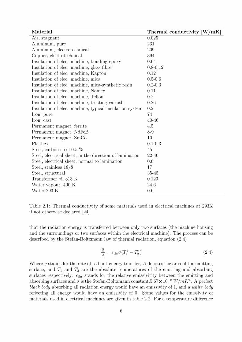
Material Thermal conductivity [W/mK]Air, stagnant 0.025Aluminum, pure 231Aluminum, electrotechnical 209Copper, electrotechnical 394Insulation of elec. machine, bonding epoxy 0.64Insulation of elec. machine, glass fibre 0.8-0.12Insulation of elec. machine, Kapton 0.12Insulation of elec. machine, mica 0.5-0.6Insulation of elec. machine, mica-synthetic resin 0.2-0.3Insulation of elec. machine, Nomex 0.11Insulation of elec. machine, Teflon 0.2Insulation of elec. machine, treating varnish 0.26Insulation of elec. machine, typical insulation system 0.2Iron, pure 74Iron, cast 40-46Permanent magnet, ferrite 4.5Permanent magnet, NdFeB 8-9Permanent magnet, SmCo 10Plastics 0.1-0.3Steel, carbon steel 0.5 % 45Steel, electrical sheet, in the direction of lamination 22-40Steel, electrical sheet, normal to lamination 0.6Steel, stainless 18/8 17Steel, structural 35-45Transformer oil 313 K 0.123Water vapour, 400 K 24.6Water 293 K 0.6

Table 2.1: Thermal conductivity of some materials used in electrical machines at 293Kif not otherwise declared [24]

that the radiation energy is transferred between only two surfaces (the machine housingand the surroundings or two surfaces within the electrical machine). The process can bedescribed by the Stefan-Boltzmann law of thermal radiation, equation (2.4)

q

A= εthrσ(T 4

1 − T 42 ) (2.4)

Where q stands for the rate of radiant-energy transfer, A denotes the area of the emittingsurface, and T1 and T2 are the absolute temperatures of the emitting and absorbingsurfaces respectively. εthr stands for the relative emissivitity between the emitting andabsorbing surfaces and σ is the Stefan-Boltzmann constant,5.67×10−8 W/mK4. A perfectblack body absorbing all radiation energy would have an emissivity of 1, and a white bodyreflecting all energy would have an emissivity of 0. Some values for the emissivity ofmaterials used in electrical machines are given in table 2.2. For a temperature difference

6

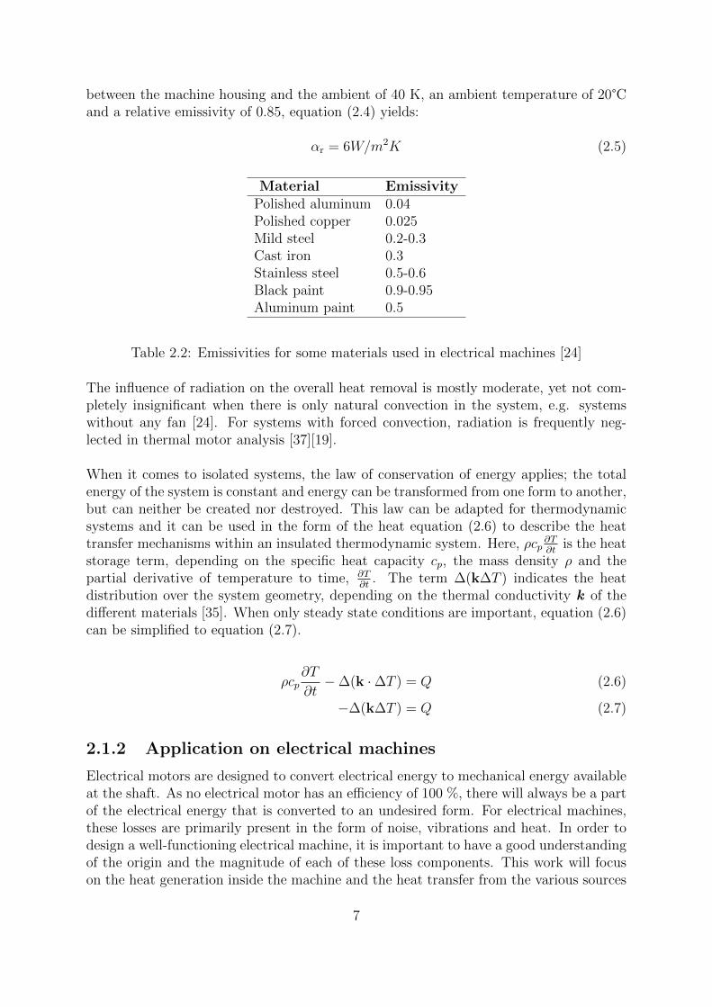
between the machine housing and the ambient of 40 K, an ambient temperature of 20°Cand a relative emissivity of 0.85, equation (2.4) yields:

αr = 6W/m2K (2.5)

Material EmissivityPolished aluminum 0.04Polished copper 0.025Mild steel 0.2-0.3Cast iron 0.3Stainless steel 0.5-0.6Black paint 0.9-0.95Aluminum paint 0.5

Table 2.2: Emissivities for some materials used in electrical machines [24]

The influence of radiation on the overall heat removal is mostly moderate, yet not com-pletely insignificant when there is only natural convection in the system, e.g. systemswithout any fan [24]. For systems with forced convection, radiation is frequently neg-lected in thermal motor analysis [37][19].

When it comes to isolated systems, the law of conservation of energy applies; the totalenergy of the system is constant and energy can be transformed from one form to another,but can neither be created nor destroyed. This law can be adapted for thermodynamicsystems and it can be used in the form of the heat equation (2.6) to describe the heattransfer mechanisms within an insulated thermodynamic system. Here, ρcp

∂T∂t

is the heatstorage term, depending on the specific heat capacity cp, the mass density ρ and thepartial derivative of temperature to time, ∂T

∂t. The term ∆(k∆T ) indicates the heat

distribution over the system geometry, depending on the thermal conductivity k of thedifferent materials [35]. When only steady state conditions are important, equation (2.6)can be simplified to equation (2.7).

ρcp∂T

∂t−∆(k ·∆T ) = Q (2.6)

−∆(k∆T ) = Q (2.7)

2.1.2 Application on electrical machines

Electrical motors are designed to convert electrical energy to mechanical energy availableat the shaft. As no electrical motor has an efficiency of 100 %, there will always be a partof the electrical energy that is converted to an undesired form. For electrical machines,these losses are primarily present in the form of noise, vibrations and heat. In order todesign a well-functioning electrical machine, it is important to have a good understandingof the origin and the magnitude of each of these loss components. This work will focuson the heat generation inside the machine and the heat transfer from the various sources

7

to the cooling system. During operation of an electrical motor, heat will mainly originatefrom resistive losses due to electrical currents in the windings (copper losses) and fromthe iron losses in the yokes of the machine. These iron losses are caused by hysteresiseffects and eddy currents in the electrical steel [16]. Other sources of heat are e.g. frictionlosses in bearings and slip ring contacts, if present, or magnet losses when the machine isequipped with permanent magnets. In steady state conditions, all heat generated in theinterior of the machine will be transferred by a combination of conduction and convec-tion (and, as mentioned before, to a negligible extend by radiation) to the cooling system.

These processes can be described by a thermal model of the machine. Such a model cangive insight in the heat flow inside the machine and can be used to predict the temperat-ure of various machine components in different operating points. This knowledge can beused to increase the power output of a certain machine without shortening the lifetime,or to design more compact machines with the same power rating. Additionally, a betterunderstanding of the internal temperature distributions will help to improve the designof the cooling system and to attain a higher overall machine efficiency. A thermal modelis thus a valuable tool to ensure that the machine is controlled in safe operating areas ofspeed and torque that will result in internal temperatures below the critical temperatureof the different machine components. Additionally, the thermal model can highlight pos-sibilities to improve the thermal design as well.

Thermal failure will in most cases occur in the windings. Therefore, peak slot or end-winding temperatures must remain below the designated insulation class limit. Whenoperated above these limits for longer periods of time, the lifetime of the winding insu-lation will decrease considerably. Exposure to peak temperatures can lead to electricalbreakdown of the insulation of the windings which will result in a short-circuit. Othernegative effects of high internal temperatures are possible distortion and thermal fatigueof rotors, stator, housing and bearings. Additionally, the use of highly temperature sens-itive materials in electrical machines, such as neodymium-iron-boron permanent magnets,lead to a lower tolerance to thermal overload as these can be permanently demagnetizedwhen exposed to temperatures that are too high. Furthermore, the lifetime of the windinginsulation will decrease considerably when the machine is operated above the temperat-ure limits for longer periods of time. Finally, the energetic efficiency of the machine willbe lower at elevated temperatures due to increased winding resistances and reduced mag-netic susceptibility of the iron in the yokes as well. This non-exhaustive listing stressesthe importance of an accurate thermal model, in particular when high torque and powerdensities are being pursued in the machine design, as the margin for error is then oftensmall [19].

Now the basic heat transfer modes and the importance of an accurate thermal modelhave been explained, the different modes of heat transfer can be modelled to describe theheat transfer mechanisms inside an electrical machine. In literature, mainly two differentapproaches are described. A first possibility is the use of a so called Lumped Parameter -model [19] [20]. In a model of this kind, the electrical machine is divided into a numberof subdomains in which simplifying assumptions with respect to the heat transfer areadopted. The heat flow between these regions is calculated using an equivalent thermal

8

circuit in which thermal parameters such as temperature, heat flux and thermal resistanceare represented by their respective electrical counterparts (see table 2.3); voltage, currentand resistance [13]. These regions are modelled as thermal nodes having a bulk thermalstorage, a heat source and interconnections to neighbouring components through a lin-ear mesh of thermal resistances [19]. These resistances are calculated using the machinegeometry and the thermal properties of the materials as well as the flow in the machine.The nodes approximate the mean temperature within the corresponding component. Theheat generation due to losses is introduced as a point source in the corresponding node.An example of such a thermal circuit is shown in figure 2.1. These circuits can be solvedwith the nodal point method as is used in common circuit theory or with general circuitanalysis software such as e.g. Spice [24] to obtain both a steady-state and a transientsolution for the temperature distribution within the electrical machine. For a good ac-curacy, the number of nodes has to be high enough to include the major componentsand heat transfer mechanisms in the machine. The lumped-parameter approach requireslittle computational effort and offers the possibility to include both radial and axial heatflow but is however based on many assumptions.

The second approach for the thermal analysis of an electrical machine is the use of fi-nite element methods (FEM). In this kind of model, a mesh is fitted over a physicalrepresentation of the machine and subsequently, material properties are assigned to thedifferent parts of the machine model and the proper boundary conditions are allocatedto the edges of the machine geometry. When the model is meant to be used for transientanalysis, the starting conditions of the system need to be specified as well. The differentloss components can be introduced as volumetric heat sources in the corresponding modelsections. The thermal problem is solved by evaluating the heat equation (2.6) for all de-grees of freedom, resulting in a temperature distribution over the machine geometry. Anexample of a temperature distribution obtained using a FEM model is shown in figure2.2. The physical representation can be a 2D or 3D geometrical model of the machine,although most models in literature only use a 2D geometry to limit computation timesand because the most important heat flow is in the radial direction only [27][31]. Heatflow in the axial direction can be modelled to a certain extent with a 2D representationas well; this will be explained further on in chapter 3, where the FE thermal model ofthe prototype EVT is discussed. Finite element methods offer more detailed models,especially when they are combined with electromagnetic FEM models for accurate lossdetermination [7]. Notwithstanding the advancements in FEM software packages andthe increased availability of computational force, the accuracy of FEM models is stilldepending on the quality of the various input parameters for the model, e.g. solid ma-terial properties, machine geometry and fluid properties. For numerous applications, theaccuracy is nowadays predominantly determined by the quality of this input data.

9

Thermal flow Unit Electric flow UnitQuantity of heat J Electric charge CHeat flow rate W Electric current AHeat flow density W/m2 Current density A/m2

Temperature K Electric potential VTemperature rise K Voltage VThermal conductivity W/mK Electric conductivity σThermal resistance K/W Electric resistance ΩThermal conductance W/K Electric conductance SHeat capacity J/K Capacitance F

Table 2.3: Thermal quantities and their electrical counterparts [24]

Figure 2.1: Thermal equivalent circuit of a typical electrical machine [24]

10

(a) FEM mesh (b) temperature distribution

Figure 2.2: FEM thermal model

11

2.2 Thermal properties of important machine com-

ponents

2.2.1 Contact resistances

In order to have an accurate thermal model, it is not sufficient to regard only correctthermal material properties. These properties are important to describe the heat flowthrough the different materials in the machine, but it is necessary to include the thermalcontact resistances at the interface of two different machine components as well. Thesecontact resistances can be found at several locations inside electrical machines [7][31][19]

• stator-frameThe stator to frame interface lies on the main heat flow path of the stator losses tothe ambient air or water jacket if present. Due to the rough surface of the statorlaminations at the interface with the machine housing, the thermal resistance willbe non-zero. Its value is a function of the pressure created by the shrink fit.

• winding-slotThe bare conductor strands are insulated with a coating, while the total winding isinsulated as a whole from the yoke by the slot insulation. In most cases, the con-ductor strands are not modelled individually, but the complete winding is modelledby an equivalent material (see subsection 2.2.4). However, the slot insulation ma-terial and the contact resistance of the insulation-yoke interface have to be modelledseparately from the equivalent winding material.

• bar-slotWhen a winding is made out of bars, the contact resistance between these bars andthe surrounding yoke is determined by the embedding.

• rotor yoke-shaftWhen there is heat generation in a rotor, the heat path through the shaft and anybearings has to be modelled. Thereby a thermal contact resistance between rotorand shaft has to be considered.

• permanent magnets – yokeIn machines with permanent magnets, there is a thermal barrier between the yokeand the magnet material due to the fixation of the magnets to the yoke. Thisbarrier can e.g. be a layer of glue. This barrier will play a role when the lossesin the magnets are included in the model. This can be necessary for temperaturedependent magnet materials, such as neodymium-iron-boron.

• rotor bandageThe supporting bandage around rotors of high speed machines forms a thermalbarrier between the rotor yoke with the winding and the air gap.

These contact resistances can be incorporated in the FEM thermal model in differentways. A possible approach is to include the thermal resistance in the material propertiesby using a single equivalent material. When using an equivalent thermal conductivity,

12

the temperature at the layer surface will be correct but the temperature distribution inthe bulk material will deviate. Nevertheless, the average temperature will be calculatedcorrectly. This approach offers the advantage of a clear geometrical relation between themodel and the actual machine [7]. Another possibility is to model the contact resistanceby means of a thin air gap [31]. Further on in this work, it will be specified how andwhen contact resistances are incorporated into the FEM thermal model.

2.2.2 Thin material layers

When looking at the geometry of electrical machines, one can discern multiple thin ma-terial layers. Although these layers are geometrically negligible, some of them play a keyrole in the thermal behaviour of the machine. A first important thin layer is the insula-tion layer between the copper windings and the yoke. As the copper losses are generatedin the windings, the insulation layer has a great influence on the hot spot temperature inthe windings [31] and the heat transfer to the yoke. A second example of a thin layer arethe air gaps between stator and rotor or between two rotors. For machines with consid-erable heat generation in the rotor, the airgap lies on an important heat flow path to thesurroundings or the cooling system. It is thus important that these layers are modelledwith appropriate consideration, regardless of their geometrical dimensions.

In FEM models, thin layers can be problematic. When the dimensions of the meshelements equal the dimensions of the layer, this can be troublesome. If the modelledgeometry is large compared to the layer, rounding errors will make the nodal coordinatesof the layer elements almost identical. This will lead to badly conditioned elements andhas to be avoided [7]. Possible solutions are to refine the mesh in those areas or to rescalethe dimensions in the layers. This implies that thermal conductivities and possible heatsources need to be rescaled accordingly. In this work, the mesh will be refined in the thinlayers that are present in the electrical machine here considered.

2.2.3 End winding convection

When a radial 2D representation of the electrical machine is used in the FEM model, onlythe parts of the windings in the slots are modelled. The copper losses are then assumedto be generated uniformly in the copper volume in the slots. The end winding regionshowever, contribute to the heat transfer as well. When axial air cooling is applied, therewill be forced convection heat transfer between the end windings and the air flowingthrough the machine. If no axial air cooling is applied, a natural convection between theend windings and the surrounding air will be noticed. This phenomenon can be modelledwith a convective heat transfer coefficient and a scaling factor for the winding surface nor-mal to the radial plane. The surface that will participate in the convective heat transferis the sum of all outer surfaces of a toroid structure and short cylindrical extensions of theslot windings. This contact area can be calculated based on the construction drawings ofthe machine and is increased by 50 % to include the surface irregularities and the greaterarea of the flatter structure of a true endwinding [19]

With the obtained geometrical factor, the thermal convective heat coefficient can be

13

scaled. This coefficient can then be used in the model as a boundary condition in theaxial direction. In this way it is possible to accommodate for the axial heat flow evenwhen the model is only two-dimensional.

2.2.4 Model of the slot windings

A variety of winding topologies can be found in electrical machines. These windingsusually consist of multiple materials such as the conductor material, the conductor in-sulation (commonly referred to as enamel), and impregnation insulation material suchas a varnish or epoxy, and possible air inclusions. Most windings are constructed withmultiple individual aluminum or copper conductors with circular or rectangular crosssections. Depending on the winding process, the winding can be loose or more firm, andthe conductor arrangement can be random or orderly. The impregnation material can beair for less demanding applications, but more advanced machine designs make use of avarnish or epoxy potting to improve electrical, mechanical and thermal properties of thewinding. These impregnated windings require more complicated production processesand the use of additional materials, which make them more expensive compared to non-impregnated windings. The impregnation provides mechanical support and enhances thethermal conductivity of the winding amalgam however. Due to the multitude of differentmaterials in the winding amalgam and the variety of possible configurations, electricalwindings are one of the more challenging machine parts when it comes to thermal mod-elling. In addition, a major part of the heat generated due to losses inside an electricalmachine find their origin in the conductors in the windings. As the insulation lifetimeis an exponential function of the peak operating temperature, hotspot temperatures ex-ceeding the thermal limits will significantly reduce the lifetime of the machine and mayeven lead to insulation breakdown and short circuiting of the winding. Furthermore, thematerial in the direct vicinity of the conductors has a large influence on the thermalproperties of the composite winding. The use of certain impregnation techniques forexample, can increase the thermal capacity of the winding considerably when comparedto air-surrounded windings. This will alter the temperature distribution in the windingregion so that some machines can be submitted to short periods of overload [13]. It isthus important to accurately predict the temperature distribution in the winding regionin the design stage of an electrical machine. Therefore it is necessary that the compositeelectrical winding is well modelled.

Due to the composite nature of an electrical winding, the thermal properties are highlyanisotropic. Because of the very high thermal conductivity of the conductor material(kCu=385 W/mK, kAl=234 W/mK) compared to the insulation materials (k=0.2 .. 1),the equivalent thermal conductivity in the axial direction is assumed to be equal to thatof the conductor material. The heat transfer in the radial direction however, is muchmore difficult to represent, as the conductor sections are insulated from each other bythe insulation materials.

Several approaches to model electrical windings have been proposed in literature. Themost straightforward approach would be to model each individual conductor and all ma-terials present in the winding amalgam using a FEA. This approach has some pronounced

14

drawbacks however, as such model is very demanding with respect to set-up times andcomputational efforts due to the detailed model geometries. Additionally, it is not alwayspossible to model the exact placing of every conductor in the winding, as the internalstructure of the winding is not always known. This is for example the case for randomlywound windings or windings made from conductors that are transversally transposed(e.g. Litzwire). FEM models in which each individual conductor within the winding isconsidered are used in literature to generate benchmark data to validate other, more con-venient approaches [29][27][36][4]. When used in thermal modelling on a higher level, thisapproach would prove to be too complex and to have too long solution times for a prac-tical application in transient analysis or iterative design and optimization procedures [29].

Other approaches attempt to describe the winding amalgam with a simplified equivalentor lumped parameter model. Different methods have been described in literature [29]

• layered winding models

• the use of a composite thermal conductivity to describe the winding region

• lumped-parameter methods.

These methods have in common that they use equivalent thermal properties of the wind-ing amalgam in some way. The accuracy is thus dependent on how accurately theseequivalent properties reflect the thermal properties of the actual winding. Ideally, exper-imental data of the electrical machine that is subject of the thermal analysis is available.Such empirical measurements of thermal properties include factors such as impregnationgoodness, insulation thickness variations and manufacturing methods, which are hard orimpossible to include in analytical or numerical models. Therefore empirically obtaineddata are preferred to include in the thermal model of electrical machines. It is howeverexpensive and time consuming to fabricate winding samples and to conduct these tothermal experiments. For this reason it is important to have other analytical or numer-ical methods to estimate equivalent thermal properties of the winding, particularly sowhen the thermal model will be used in an iterative design or optimization procedure toanalyze e.g. effects of different insulation systems, conductor shapes and dimensions ora variable packing factor.

One possibility to avoid expensive and time consuming sample manufacturing is the useof analytical homogenization procedures. These techniques have short computation timesthanks to their analytical nature and are widely used in thermal modelling of electricalwindings. The most basic form of analytical homogenization are the expressions for seriesand parallel positioning of different materials in a composite material, eqs. (2.8) and (2.9)respectively.

ke =k1k2

v1k2 + v2k1

(2.8)

ke = v1k1 + v2k2 (2.9)

Here, ke, k1, k2 and v1 and v2 are the total equivalent thermal conductivity, the thermalconductivities of the different materials and their respective volume ratios (v1 + v2 = 1)

15

[29]. As these expressions are based on the electrical counterpart of the thermal circuitas explained in subsection 2.1.2, they offer an intuitive understanding. They are how-ever not useful to describe discrete inclusions in a matrix accurately, as e.g. individualconductors surrounded by a potting material. A better analytical expression (2.10) hasbeen developed by Hashim and Shtrikman in the context of research on composite ma-terials. This expression can be used to estimate the equivalent thermal conductivity ofa composite winding with round conductor profiles consisting of two different materials[29].

ke = kp(1 + vc)kc + (1− vc)kp

(1− vc)kc + (1 + vc)kp

(2.10)

Here, kc and kp stand for the conductor and potting thermal conductivity and vc andvp denote the respective volumetric ratios, with vc + vp = 1. The volume ratio of theconductors in the amalgam is also referred to as the packing or fill factor PF and FF.Electrical windings mostly consist of three different materials however; the conductormaterial, the enamel and the impregnation material or potting. To overcome this problem,adaptations to the Hashin and Shtrikman expression have been proposed by Simpson [29].In order to account for a third material, the enamel and the impregnation material arerepresented by a parallel model and (2.10) is adjusted with equations (2.11) to (2.17).

ka = kiivii

vii + vci+ kci

vcivii + vci

(2.11)

vc + vci = PF (2.12)

vc + vci + vii = 1 (2.13)

vii = (1− PF ) (2.14)

vc = PF · r2c

(rc + li)2(2.15)

vci = PF · 2rcli + l2i(rc + li)2

(2.16)

ke = ka(1 + vc)kc + (1− vc)ka(1− vc)kc + (1 + vc)ka

(2.17)

Here, the subscripts ii and ci denote the impregnation insulation and the conductorinsulation, while rc and li represent the conductor radius and the insulation thickness.Equations (2.11) and (2.14)to (2.16) are evaluated for a value of the packing factor PFand substituted in (2.17). In this way, the three materials that are present in the windingamalgam can be represented using the Hashin and Shtrikman approximation.

Another possibility to adapt the Hashin and Shtrikman approximation for applicationswith three different materials is to assume comparable thermal properties for the enameland the impregnation material. In that case, the three-material composite can be reducedto a two-material system. This approach lead to accurate results in [27] (kenamel=0.26,kpotting=0.21) but to an overestimation of the equivalent thermal conductivity in [29](kenamel=0.26, kpotting=0.85). It is thus necessary that the assumption of similar thermalconductivities for both enamel and impregnation material hold when the Hashin and

16

Shtrikman approximation (2.10) is applied. The modified Hashin and Shtrikman expres-sion (2.17) on the other hand, still overestimated the equivalent thermal conductivity in[29], but to a lower extent.

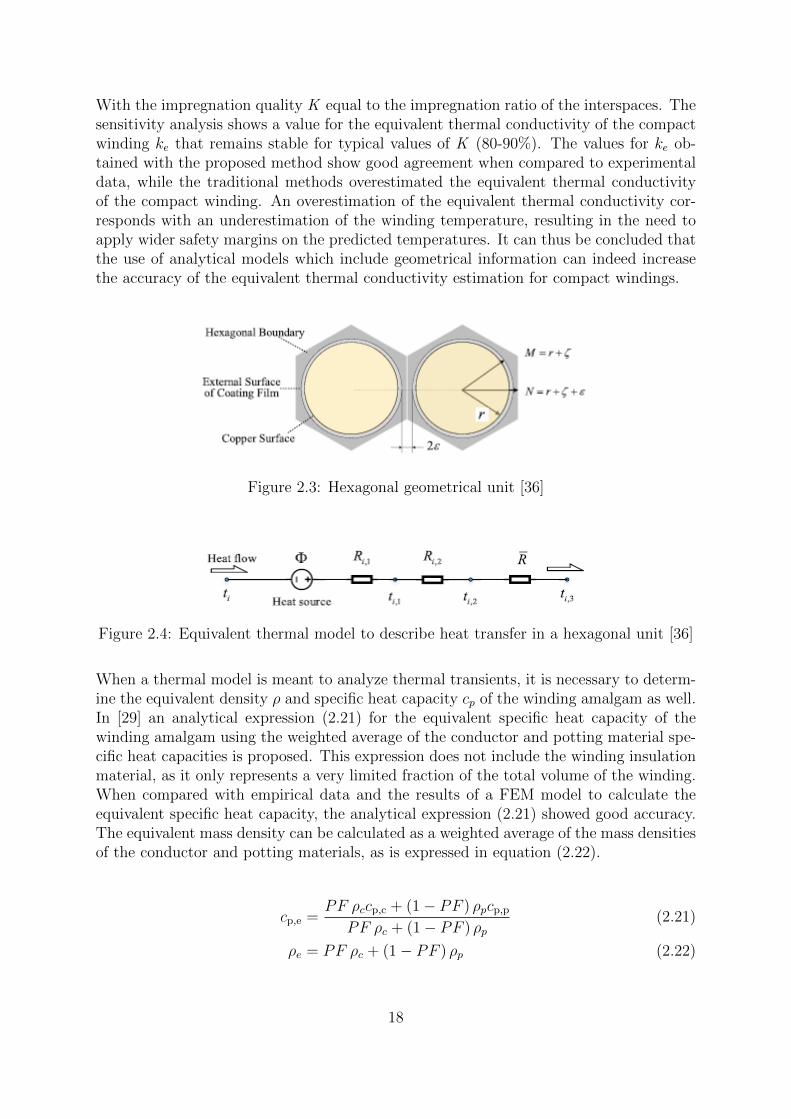
Due to an increasing demand for compact electrical machines with high power densitiesand increased speed ranges, the thermal limitations of the winding region become moreapparent. Winding designs with a maximal fill factor show improved heat dissipationand can reduce the machine frame size. Due to improvements in winding fabrication,compact electrical windings show an increased regularity in the cross section comparedto loosely and randomly wound windings. This geometrical information can possibly beused to improve the analytical homogenization methods that are traditionally used. In[36] an analytical estimation method based on hexagonal units has been proposed. Thesehexagonal units contain all different materials and take the geometrical characteristicsof the internal winding structure into account, see figure 2.3. The heat transfer processinside such a hexagonal unit is described using the equivalent thermal circuit depictedin figure 2.4. The heat source Φ is evenly distributed over the conductor cross section,Ri,1 represents the thermal resistance from the centre of the conductor to the surface,Ri,2 the thermal resistance from the conductor surface to the surface of the enamel andR represents the thermal resistance from the enamel surface to the boundary of thehexagonal unit. The equivalent thermal conductivity for the compact winding can becalculated using equations (2.18) and (2.19).

ke =

[1

kc+

2 ln(1 + ζ

r

)

kf+

4π

kgP (N/M)

]−1

(2.18)

P (η) =5.273η − 0.283

ν − 0.984(2.19)

Where ζ, r,N and M are geometrical parameters and kc, kf and kg the thermal conductiv-ities of the conductor, the enamel and the impregnation material respectively. Neverthe-less these compact windings show an increased regularity, the exact winding distributionand the impregnation quality can still deviate from machine to machine. Therefore theauthors carried out two sensitivity studies. Firstly, the effect of deformed interspaces dueto wire dislocations [figure] was examined. When conductors slip away from their regularstacking position, the interspace will increase which will affect the equivalent thermalconductivity of the winding. There will always be some dislocations present in a compactwinding, but the total percentage will be limited by space constraints and surface contactforces between the wires. Therefore the sensitivity analysis has been carried out for aproportion of generalized deformed interspaces in the range of 5 to 50 %. The resultsshow a stable value for ke, even when the exact geometry of the compact winding is un-known. Using the proposed model, ke can be determined in a small range, of which theboundary values can be calculated. Secondly, the interspaces will only be partially filledduring the impregnation process. Even more so when impregnation materials with higherviscosities (e.g. impregnation materials with higher thermal conductivity) are used. Forthis reason the thermal conductivity of the impregnation material used in the model isadapted with equation (2.20).

ki,e = Kki + (1−K)kair (2.20)

17

With the impregnation quality K equal to the impregnation ratio of the interspaces. Thesensitivity analysis shows a value for the equivalent thermal conductivity of the compactwinding ke that remains stable for typical values of K (80-90%). The values for ke ob-tained with the proposed method show good agreement when compared to experimentaldata, while the traditional methods overestimated the equivalent thermal conductivityof the compact winding. An overestimation of the equivalent thermal conductivity cor-responds with an underestimation of the winding temperature, resulting in the need toapply wider safety margins on the predicted temperatures. It can thus be concluded thatthe use of analytical models which include geometrical information can indeed increasethe accuracy of the equivalent thermal conductivity estimation for compact windings.

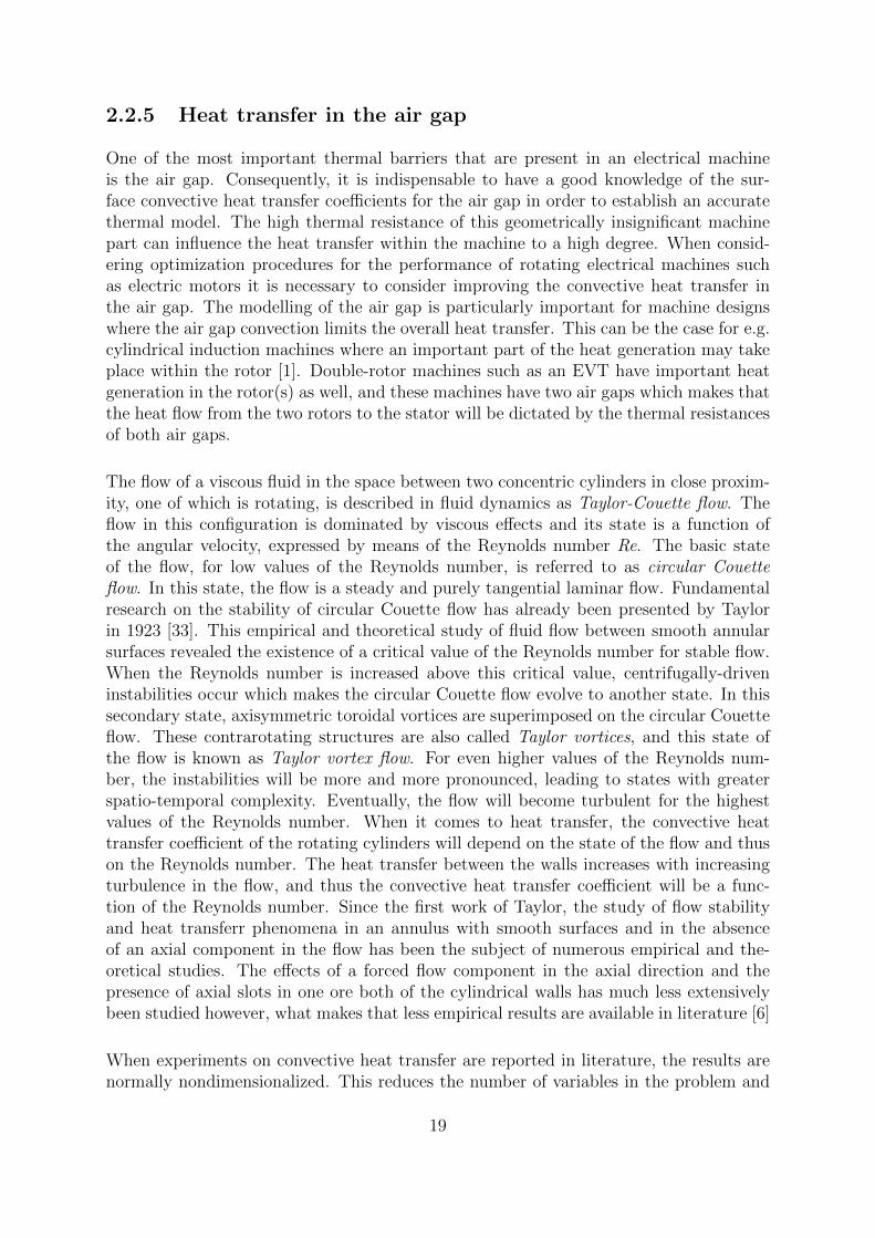
Figure 2.3: Hexagonal geometrical unit [36]

Figure 2.4: Equivalent thermal model to describe heat transfer in a hexagonal unit [36]

When a thermal model is meant to analyze thermal transients, it is necessary to determ-ine the equivalent density ρ and specific heat capacity cp of the winding amalgam as well.In [29] an analytical expression (2.21) for the equivalent specific heat capacity of thewinding amalgam using the weighted average of the conductor and potting material spe-cific heat capacities is proposed. This expression does not include the winding insulationmaterial, as it only represents a very limited fraction of the total volume of the winding.When compared with empirical data and the results of a FEM model to calculate theequivalent specific heat capacity, the analytical expression (2.21) showed good accuracy.The equivalent mass density can be calculated as a weighted average of the mass densitiesof the conductor and potting materials, as is expressed in equation (2.22).

cp,e =PF ρccp,c + (1− PF ) ρpcp,p

PF ρc + (1− PF ) ρp(2.21)

ρe = PF ρc + (1− PF ) ρp (2.22)

18

2.2.5 Heat transfer in the air gap

One of the most important thermal barriers that are present in an electrical machineis the air gap. Consequently, it is indispensable to have a good knowledge of the sur-face convective heat transfer coefficients for the air gap in order to establish an accuratethermal model. The high thermal resistance of this geometrically insignificant machinepart can influence the heat transfer within the machine to a high degree. When consid-ering optimization procedures for the performance of rotating electrical machines suchas electric motors it is necessary to consider improving the convective heat transfer inthe air gap. The modelling of the air gap is particularly important for machine designswhere the air gap convection limits the overall heat transfer. This can be the case for e.g.cylindrical induction machines where an important part of the heat generation may takeplace within the rotor [1]. Double-rotor machines such as an EVT have important heatgeneration in the rotor(s) as well, and these machines have two air gaps which makes thatthe heat flow from the two rotors to the stator will be dictated by the thermal resistancesof both air gaps.

The flow of a viscous fluid in the space between two concentric cylinders in close proxim-ity, one of which is rotating, is described in fluid dynamics as Taylor-Couette flow. Theflow in this configuration is dominated by viscous effects and its state is a function ofthe angular velocity, expressed by means of the Reynolds number Re. The basic stateof the flow, for low values of the Reynolds number, is referred to as circular Couetteflow. In this state, the flow is a steady and purely tangential laminar flow. Fundamentalresearch on the stability of circular Couette flow has already been presented by Taylorin 1923 [33]. This empirical and theoretical study of fluid flow between smooth annularsurfaces revealed the existence of a critical value of the Reynolds number for stable flow.When the Reynolds number is increased above this critical value, centrifugally-driveninstabilities occur which makes the circular Couette flow evolve to another state. In thissecondary state, axisymmetric toroidal vortices are superimposed on the circular Couetteflow. These contrarotating structures are also called Taylor vortices, and this state ofthe flow is known as Taylor vortex flow. For even higher values of the Reynolds num-ber, the instabilities will be more and more pronounced, leading to states with greaterspatio-temporal complexity. Eventually, the flow will become turbulent for the highestvalues of the Reynolds number. When it comes to heat transfer, the convective heattransfer coefficient of the rotating cylinders will depend on the state of the flow and thuson the Reynolds number. The heat transfer between the walls increases with increasingturbulence in the flow, and thus the convective heat transfer coefficient will be a func-tion of the Reynolds number. Since the first work of Taylor, the study of flow stabilityand heat transferr phenomena in an annulus with smooth surfaces and in the absenceof an axial component in the flow has been the subject of numerous empirical and the-oretical studies. The effects of a forced flow component in the axial direction and thepresence of axial slots in one ore both of the cylindrical walls has much less extensivelybeen studied however, what makes that less empirical results are available in literature [6]

When experiments on convective heat transfer are reported in literature, the results arenormally nondimensionalized. This reduces the number of variables in the problem and

19

makes it possible to apply the results to machine geometries other than the one used inthe reported experiment. The most important nondimensional groups are [1]

• the Reynolds number Re, which is a function machine size and rotational speed

• the average Nusselt number Nu, which is the nondimensional surface convectiveheat transfer coefficient

• the Prandtl number Pr, defined as the ratio of momentum diffusivity to thermaldiffusivity

• Cw, which is the nondimensional air mass flow rate through a machine

• the Taylor number Ta, which gives an indication of the relative effects of inertialforces and viscosity for an annulus with rotation of one or more of the cylindricalsurfaces

• geometric parameters such as the gap ratio G.

When using the Reynolds number and the Nusselt number, one has to specify whichcharacteristic length is used in the definition. When the rotor radius is used, thesenondimensional groups are referred to as the rotational Reynolds number Reθ and therotational Nusselt number Nuθ, whereas they are called the gap Reynolds number Reg

and the gap Nusselt number Nug when the air gap width is used as characteristic length.When the air gap length Lδ is used as characteristic length, the Reynolds number isreferred to as the axial Reynolds number Rea. For cylindrical annuli, the Nusselt numberis expressed in terms of the hydraulic diameter Dh. The various dimensionless groups aredefined as

Reg =ωδR

ν(2.23)

Reθ =ωR2

ν(2.24)

Rea =vaxialDh

ν(2.25)

Nu =hDh

k(2.26)

Pr =cpµ

k(2.27)

Dh = 2δ (2.28)

G =g

R(2.29)

Cw =m

µR(2.30)

Ta =ωa r

0.5m δ1.5

ν(2.31)

rm =a+ b

2(2.32)

20

Where R is the rotor radius, ω stands for the angular speed and ν denotes the fluidkinematic viscosity (usually at ambient temperature). h is the convective heat trans-fer coefficient, k is the fluid thermal conductivity (usually at ambient temperature), Lδ

stands for the length of air gap in the axial direction, δ is the gap size between the rotorand the stator, m is the air mass flow rate, µ denotes the dynamic viscosity of the fluidand a and b stand for the inner and outer annulus diameters respectively.

To apply a convective heat transfer coefficient to a thermal model of the air gap, theappropriate Nusselt number correlation for the situation has to be selected, e.g. Nu =AReBθ . The Nusselt number can be calculated from the correlation and subsequently,the convective heat transfer coefficient can be calculated from the Nusselt number usingequation (2.26). For lumped parameter models, a thermal resistance can be calculatedwith equation (2.33). When a FEM model is used, the thermal convective heat transfercoefficient can be applied as a boundary condition or an equivalent thermal conductivityfor the air gap subdomain can be calculated with equation (2.34) [16].

Rth =1

hA=

Dh

Akfluid Nu(2.33)

kairgap =δ

Rth A(2.34)

When considering heat transfer in the air gap of cylindrical machines which do not havea forced gas flow through the air gap, it can be assumed that the mean heat transferpath will be in the radial direction. This is generally the case for electrical machines ofthe totally enclosed type without external fan. For these machines the cooling throughthe air gap is not very effective and the heat will be transferred from the hotter rotorsurface through the air gap to the stator surface by combined effects of convection andconduction. As has been explained above, the heat transfer is a function of the state ofthe Taylor-Couette flow in the air gap. When the annular gap size δ = b − a is smallcompared to the mean radius rm, i.e. the small gap approximation holds, Taylor foundthat the angular velocity ωcrit that indicates the transition from circular Couette flow toTaylor-Couette flow equals [1]

ωcrit = π2ν

√a+ b

2S(b− a)3a2 [1− (ωb/ωa) b2/a2] (1− ωb/ωa)(2.35)

S = 0.0571

[1 + ωb/ωa1− ωb/ωa

+ 0.652(a− x)

]+ 0.00056

[1 + ωb/ωa1− ωb/ωa

+ 0.652(a− x)

]−1

(2.36)

x =b

a(2.37)

For common machine topologies with a stationary outer cylinder and a narrow air gap,ωb = 0 and a

b→ 1, thus (2.35) and (2.36) reduce to (2.38) and (2.39) which result in

(2.40) for the critical Taylor number

21

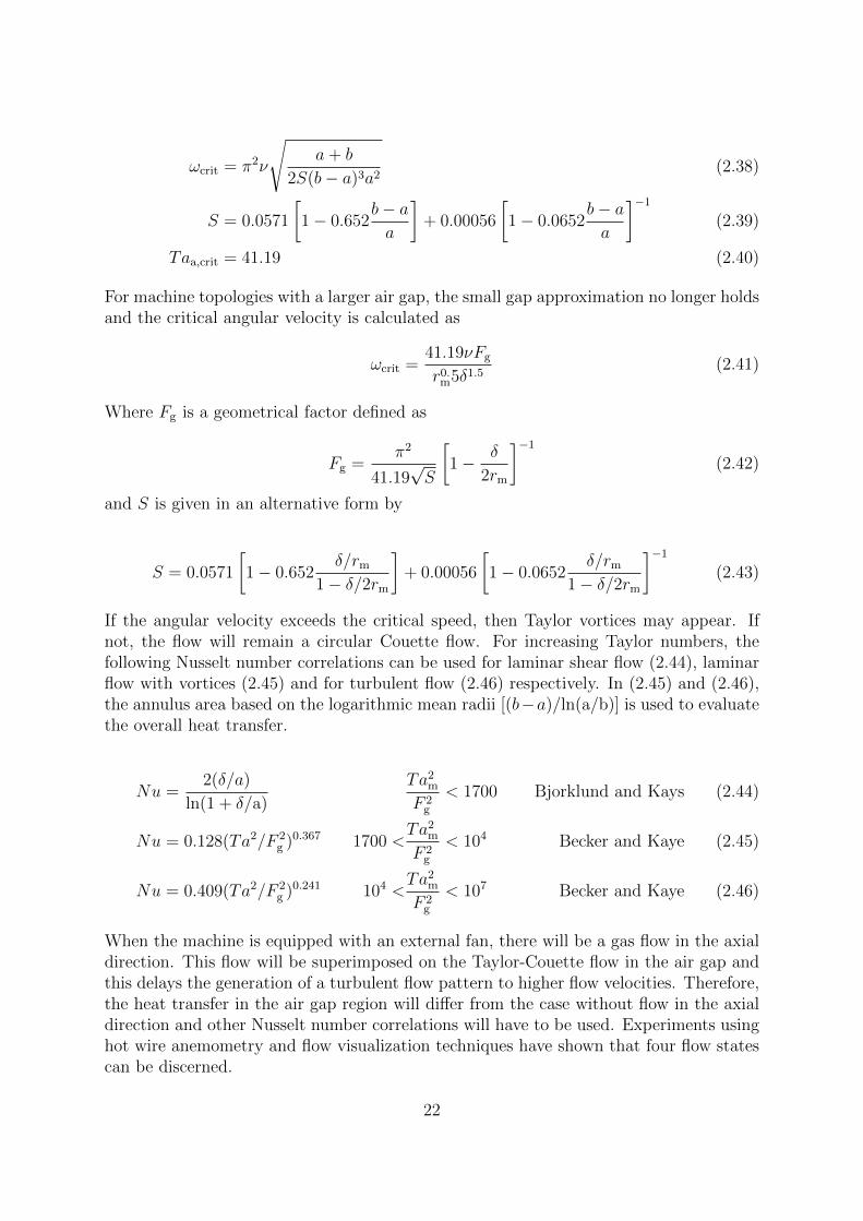
ωcrit = π2ν

√a+ b

2S(b− a)3a2(2.38)

S = 0.0571

[1− 0.652

b− aa

]+ 0.00056

[1− 0.0652

b− aa

]−1

(2.39)

Taa,crit = 41.19 (2.40)

For machine topologies with a larger air gap, the small gap approximation no longer holdsand the critical angular velocity is calculated as

ωcrit =41.19νFg

r0.m5δ1.5

(2.41)

Where Fg is a geometrical factor defined as

Fg =π2

41.19√S

[1− δ

2rm

]−1

(2.42)

and S is given in an alternative form by

S = 0.0571

[1− 0.652

δ/rm

1− δ/2rm

]+ 0.00056

[1− 0.0652

δ/rm

1− δ/2rm

]−1

(2.43)

If the angular velocity exceeds the critical speed, then Taylor vortices may appear. Ifnot, the flow will remain a circular Couette flow. For increasing Taylor numbers, thefollowing Nusselt number correlations can be used for laminar shear flow (2.44), laminarflow with vortices (2.45) and for turbulent flow (2.46) respectively. In (2.45) and (2.46),the annulus area based on the logarithmic mean radii [(b−a)/ln(a/b)] is used to evaluatethe overall heat transfer.

Nu =2(δ/a)

ln(1 + δ/a)

Ta2m

F 2g

< 1700 Bjorklund and Kays (2.44)

Nu = 0.128(Ta2/F 2g )0.367 1700 <

Ta2m

F 2g

< 104 Becker and Kaye (2.45)

Nu = 0.409(Ta2/F 2g )0.241 104 <

Ta2m

F 2g

< 107 Becker and Kaye (2.46)

When the machine is equipped with an external fan, there will be a gas flow in the axialdirection. This flow will be superimposed on the Taylor-Couette flow in the air gap andthis delays the generation of a turbulent flow pattern to higher flow velocities. Therefore,the heat transfer in the air gap region will differ from the case without flow in the axialdirection and other Nusselt number correlations will have to be used. Experiments usinghot wire anemometry and flow visualization techniques have shown that four flow statescan be discerned.

22

• purely laminar flow

• laminar flow with Taylor vortices

• turbulent flow with vortices

• turbulent flow

For the laminar flow with Taylor vortices, Simmers and Coney derived the Nusselt numbercorrelation (2.47) [28].

Nu =4Pr Re0.5

a Ta2·0.3675

B[A

1−x

]0.5 [ x1−x

]0.25Ta2·0.6175

crit

(2.47)

A =

[1 + x2 +

(1− x2

lnx

)](2 +

1− x2

lnx

)−1

(2.48)

B = Pr + ln

[1 + Pr exp

(2

3

(1− xx

)0.25(xA

(1− x)2

)0.5

Re−0.5a Ta0.265 Ta0.235

crit − 1

)− Pr

]

(2.49)

For turbulent flow with vortices, Gazley derived the Nusselt number correlation (2.50),based on a Reynolds number that uses the vector sum of the bulk axial flow velocity andthe rotor speed, Ree. Kosterin and Finatev presented the correlation (2.52) [1]

Nu = 0.03Re0.8e for Rea < 1.2 · 104 and Reθ < 1.1 · 105 (2.50)

Ree =

√v2

axial + v2θDh

ν(2.51)

Nu = 0.018[Rea

[1 + 0.6((ωa aDh/ν)/Rea)2

]0.5]0.8

for 0 <ωaaDh

ν< 105 and 3 · 103 < Rea < 3 · 104 (2.52)

For turbulent flow in an annulus of which the inner cylinder is rotating, Kuzay and Scottpresented the correlation (2.53) based on measurements conducted on a rig with a radiusratio equal to 0.57. Childs et al. and Childs and Turner presented the correlation (2.54)based on experiments on a large rotating drum with a diameter of 400 mm [1].

Nu = 0.022

[1 +

Dhvθπava

2]0.8714

Re0.8a Pr0.5 for Rea < 6.5 · 105 and Reθ < 4 · 104

(2.53)

Nu−Nux

Nux

= 0.068

(vθva

)2

for 1.7 · 105 < Rea < 3.7 · 105

and 1.4 · 104 < Reθ = ωa2/ν < 2.7 · 1061.65 < z/Dh < 5 (2.54)

Nux = 0.023Re0.8a

√Pr (2.55)

23

For other machine types, the main heat flow is in the axial direction. This is for examplethe case for high speed machines with forced gas cooling. The cooling of these types ofelectrical machines relies on a forced fluid flow in the axial direction through the airgap.This cooling strategy is characterized by the fact that the heat is mainly transferred byforced convection from the hotter stator and rotor surfaces to the fluid in the airgap andno longer from the rotor to the stator through the fluid in the airgap by combined effectsof convection and conduction. A highly turbulent flow in the airgap is preferred, as thiswill result in an increased convective heat transfer coefficient [21]. Typical peripheral ro-tor speeds are in the 100-300 m/s range and the axial velocity of the cooling gas is 20-60m/s. This corresponds with axial flow Reynolds numbers Rea in the range 4457-13370and Taylor numbers in the range 5914-13223. The convective heat transfer coefficientfor stator and rotor surfaces can be calculated using the semi-empiric Nusselt numbercorrelation given in equation (2.56). This correlation has been experimentally validatedfor rotor speeds from 30 000 to 80 000 RPM (peripheral speed 112-297 m/s) in [17]. Theauthors found that the measured heat transfer coefficients of the rotor and stator surfacesfollowed the trend predicted by the Nusselt correlation (2.56) but were generally slightlyoverestimated.

Some machine geometries have axial slots in one or both walls confining the air gap.These slots which contain the windings may notably modify the dynamic and thermalbehaviour of the flow in the air gap. It can therefore be necessary to evaluate the effectsof these slots on the heat transfer mechanisms in the air gap in the developing process ofa thermal model. Gazley has been first to investigate the flow in an annular set-up withaxial slots in the rotor or stator wall. In his set-up, the rotating cylinder was heated andthe stationary cylinder was cooled.

Nu = 0.0214 (Re0.8 − 100)Pr0.4

[1 +

Dh

Lδ

23

](2.56)

Rea =vredDh

ν(2.57)

Dh = δ

√8

3(2.58)

vred =

√ωR

2

2

+ vaxial (2.59)

(2.60)

With Lδ the axial length of the airgap, ρ the mass density of the cooling fluid and vred thereduced velocity in the helical direction in the air gap. ω stands for the angular velocityof the rotor, R is the outer radius of the rotor and vaxial denotes the axial velocity of thecooling fluid.

In addition to cylindrical electrical machines, so-called disk-type electrical machines canbe discerned as well, e.g. the axial flux permanent magnet (AFPM) brushless machine.The air gap magnetic field of these machines is oriented in the axial direction and the airgap is confined between two disk, one or both of which are rotating. The flow in the air

24

gap is driven by a pressure difference caused by the rotation of the rotor(s), and is thusfundamentally different from the air gap flow in cylindrical machines, where any axial flowcan only be present as the result of an externally imposed pressure difference. Therefore,the heat transfer mechanisms within the air gap will be different as well, and other Nusseltnumber correlations have to be applied, see e.g. [1]. These machine geometries are notwithin the scope of the present work however, and are thus not discussed in more detail.

25

Chapter 3

Thermal model of the EVT

3.1 The electrical variable transmission with hybrid

excitation

In [8] an EVT is described as “an electromagnetic power split transmission, having twomechanical and two electrical ports. A power split transmission converts mechanicalinput power from a prime mover by means of two different paths. An EVT transfersmechanical power from an input shaft to the output shaft by means of an electric andan electromagnetic path. ” It is a sort of rotating electrical machine with two concentricshafts and two electrical connections with the grid and/or with an external energy storage.

Two possible applications of an EVT system are its use as a series-parallel power splittransmission system for hybrid electrical vehicles [9] and the implementation of an EVTsystem as a shaft-to-shaft CVT [14][15]. As a power split transmission system, an EVTcan be applied in hybrid electric vehicles such as passenger cars and city busses, but alsoin railway and maritime driving systems [11]. When used as a power split transmissionsystem, the EVT with hybrid excitation offers the possibility to transfer the power to theload by two different paths. The power delivered by a primary mover that is connectedto the input shaft of the EVT can be transferred to the load that is connected to theoutput shaft of the EVT through electromagnetic forces. The remainder of the the powerdemanded by the load can then be delivered through power electronic converters con-nected to the windings of the EVT, what makes that these power electronic componentscan be dimensioned for a lower power rating. This is not the case for e.g. Diesel-Electricsystems, where the full output power needs to be converted by two power electronicconverters (e.g. rectifier and inverter) and two electrical machines (e.g. generator andelectric motor). When compared to mechanical CVT systems such as a push-belt CVTor a half-toroidal CVT, the EVT has some inherent advantages that are characteristicfor electromagnetic devices [8]

• low maintenance due to the absence of mechanical power transferring contacts

• built-in overload protection due to the electromagnetic nature of the torque trans-mission

• no need for a reversing unit as the system can operate with negative gear ratios

26

• no need for a clutch as one shaft can be at standstill while the other is rotating

• a higher efficiency

• faster dynamics.

Different topologies of EVT’s are described in literature; the working principle can bebased on induction machines or on synchronous machines. In the former case, the rotorshave squirrel cages and the rotor torques depend on the slip frequencies. In the lattercase, (part of) the magnetic flux is provided by permanent magnets. This dissertationwill focus on the electrical variable transmission with hybrid excitation and more spe-cifically on a prototype built by the Dutch company Electric Variable Transmission BVthat is used in the test set-up of EELAB at Ghent University. As stated before, thismachine has two concentric rotors and a stator. Both rotors are connected to a differentshaft, which form the two mechanical ports of the system. The stator and the inner rotorare equipped with a three-phase winding. Each three-phase winding is connected to aninverter and theses inverters are connected back-to-back to a common DC bus. Theyform the two electrical ports of the four-port system. As the prototype EVT has beendesigned for application in hybrid electric vehicles, the designers aimed at a high torquedensity. Permanent magnet EVTs tend to have higher power and torque densities thaninduction machine based EVTs, especially when combined with water cooling [14]. TheEVT considered in this work is indeed equipped with permanent magnets on the insideof the outer rotor. To facilitate stator flux weakening in order to reduce iron losses andstator inverter requirements at high speeds, the outer rotor has a DC winding as well.This winding can be used to control the saturation in the part of the outer rotor yokeunderneath the DC winding (the so called ‘flux bridge’) and so the level of flux linkageof the inner rotor with the stator [9]. Due to both the permanent magnets and the DCwinding, this EVT topology is referred to as ‘hybridly excited’.

This EVT can for example be used to decouple a load with varying speed and torquelevels from a prime mover which is controlled in a fixed optimal operating point. Poweris transferred from the prime mover connected to the inner rotor to the load connectedto the outer rotor by the electromagnetic interaction between the current in the innerrotor winding and the magnetic flux coupled with the inner rotor windings. The torquedifference between both is delivered by the stator torque which originates from the elec-tromagnetic interaction between the three phase current in the stator winding and themagnetic flux coupled with this winding. The presence of the stator makes that theinput torque and speed can differ from the output torque and speed. The load is thusdecoupled from the prime mover and input and output power does not have to be equal.This additional power is exchanged with an external energy source through power elec-tronic converters. An example of such a source is the battery of a hybrid electric vehicle.

As previously stated, one of the objectives of this dissertation is the development of athermal model of this prototype EVT with hybrid excitation. This thermal model willbe part of a larger set of design tools, which will facilitate the design and development ofapplication-specific EVT systems. This implies the use of a parametric and thus scalablemachine geometry in the modelling process. As the model will eventually be integrated

27

in an overarching framework, it has to be compatible with previously created tools suchas the electromagnetic model and the loss model developed in [8]. Therefore, it has beendecided to create a FEM thermal model for the EVT using the simulation software ComsolMultiphysics together with Matlab. The temperature distribution can be calculated withthe Heat Transfer by Conduction equation system, which solves the heat equation (2.6)for every mesh point. In this process, all geometry regions are treated as solid materials.In a first step, the thermal analysis of the EVT with hybrid excitation will be limited toa two dimensional model, as the most important paths for the heat transfer within theEVT lies in the radial plane from the different windings and yokes to the water jacketcooling at the outer surface of the stator. This model will assume a constant temperaturedistribution in the axial direction and will not yet take the forced air cooling in the axialdirection into account. The model geometry will be based on the machine geometryused for the electromagnetic modelling, which will be adapted to include all importantparameters for the thermal analysis. The different heat sources in the thermal modelwill be defined by the loss model established in [8], which offers a detailed analysis of thedifferent loss components depending on the operating point of the EVT. With a transientanalysis in mind, short calculation times for the FEM model are aimed for. To thisend, the symmetry will be exploited to reduce the model geometry as much as possible.The development of this FEM model consists of the following steps: define an adequatemachine geometry, determine the thermal conductivities for all subdomains in the model,integrate the loss model into the thermal model and allocate the appropriate boundaryconditions. These steps will be discussed in detail in the remainder of this chapter.

3.2 Geometry

The prototype EVT has four pole pairs, this means that 360 electrical degrees correspondwith 360/4=90 mechanical degrees. Both copper and iron losses in an electrical machineare equal in the sections from 0°to 180°electrical and from 180°to 360°electrical. Thecomplete machine can thus be modelled using a section of 45°electrical, or 1/8 of thereal machine geometry. The heat source distribution and heat transfers in the completemachine have a symmetry axis each 180°electrical or 45°mechanical. These symmetry axiscan be modelled with well-chosen boundary conditions (see section 3.5). The geometryused in the thermal model is based on the geometry used in the electromagnetic modelof the EVT [8]. To include all important parameters for the thermal analysis however,the geometry is adapted as follows.

• The copper losses are assumed to be distributed evenly over the winding crosssection. Therefore, the complete slot surface of the double layer windings is treatedas one subdomain in the thermal model.

• The thin insulation layer surrounding each winding (i.e. the slot liner) has not beenincluded in the electromagnetic model, as its effect is insignificant. The effect ofthis layer on the heat transfer between winding and yoke is very important however,so it is included in the thermal model.

• The machine housing and the surrounding water jacket are not included in thethermal model as separate subdomains. The heat removal potential of the coolant

28

flow in the water jacket is high but the heat flow from stator yoke to the water jacketwill be limited by the thermal resistance of the rough interface between stator yokelaminations and the machine housing. To accurately model this limitation, theeffect of the yoke-housing interface and the housing material on the heat transferin the EVT is combined in a single parameter. This parameter is used to define theboundary condition on the outer surface of the stator yoke, see section 3.5.

• The yoke of the inner rotor is connected to one of the two shafts of the EVTprototype by means of an aluminum annulus with axial holes. This component isattached to the shaft on its inner surface and to the rotor yoke on its outer surface.As was the case for the slot liner material, this central annulus does not affect theelectromagnetic phenomena and is thus not included in the electromagnetic model.This component is situated on the heat transfer path from the inner rotor to the airin the axial holes, which facilitate forced air cooling in the axial direction, and onthe path from the inner rotor to the shaft and eventually the ambient. Therefore,its influence on the internal heat distribution of the EVT will not be insignificantand the component is included in the thermal model geometry. The circumferentialdistribution of the axial holes in the annulus is not exactly symmetrical for eachsegment of 45 °, but this is disregarded in the model geometry.

Prior to solving the heat equation, a mesh is fitted over the machine geometry. As stressedin subsection 2.2.2, it has to be ensured that this mesh is fine enough in the thin materiallayer subdomains within the machine geometry (i.e. the slot liner and the air gaps). Anoverview of the different subdomains of the model geometry is given in table 3.1.

SubdomainStator yokeInterrotor yokeInner rotor yokeStator slot windingsDC windingInner rotor slot windingsSlot linerAir gap stator-interrotorAir gap interrotor-inner rotorPermanent magnetsCentral annulusAxial holes

Table 3.1: Subdomains of the thermal model geometry

3.3 Thermal material properties

As has been mentioned earlier, the quality of the simulations obtained with modern FEMsoftware packages is predominantly reliant on good input data. For the solid domain

29

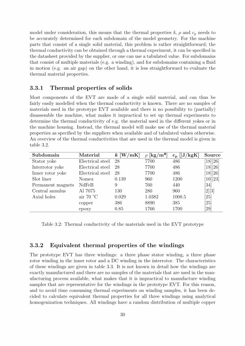
model under consideration, this means that the thermal properties k, ρ and cp needs tobe accurately determined for each subdomain of the model geometry. For the machineparts that consist of a single solid material, this problem is rather straightforward; thethermal conductivity can be obtained through a thermal experiment, it can be specified inthe datasheet provided by the supplier, or one can use a tabulated value. For subdomainsthat consist of multiple materials (e.g. a winding), and for subdomains containing a fluidin motion (e.g. an air gap) on the other hand, it is less straightforward to evaluate thethermal material properties.

3.3.1 Thermal properties of solids

Most components of the EVT are made of a single solid material, and can thus befairly easily modelled when the thermal conductivity is known. There are no samples ofmaterials used in the prototype EVT available and there is no possibility to (partially)disassemble the machine, what makes it impractical to set up thermal experiments todetermine the thermal conductivity of e.g. the material used in the different yokes or inthe machine housing. Instead, the thermal model will make use of the thermal materialproperties as specified by the suppliers when available and of tabulated values otherwise.An overview of the thermal conductivities that are used in the thermal model is given intable 3.2.

Subdomain Material k [W/mK] ρ [kg/m³] cp []J/kgK] SourceStator yoke Electrical steel 28 7700 486 [18][26]Interrotor yoke Electrical steel 28 7700 486 [18][26]Inner rotor yoke Electrical steel 28 7700 486 [18][26]Slot liner Nomex 0.139 960 1200 [10][23]Permanent magnets NdFeB 9 760 440 [34]Central annulus Al 7075 130 280 960 [2][3]Axial holes air 70 °C 0.029 1.0382 1008.5 [25]

copper 386 8890 385 [25]epoxy 0.85 1766 1700 [29]

Table 3.2: Thermal conductivity of the materials used in the EVT prototype

3.3.2 Equivalent thermal properties of the windings

The prototype EVT has three windings: a three phase stator winding, a three phaserotor winding in the inner rotor and a DC winding in the interrotor. The characteristicsof these windings are given in table 3.3. It is not known in detail how the windings areexactly manufactured and there are no samples of the materials that are used in the man-ufacturing process available, what makes that it is impractical to manufacture windingsamples that are representative for the windings in the prototype EVT. For this reason,and to avoid time consuming thermal experiments on winding samples, it has been de-cided to calculate equivalent thermal properties for all three windings using analyticalhomogenization techniques. All windings have a random distribution of multiple copper

30

conductors and are impregnated with an epoxy resin. The conductors are insulated witha polyamide-imide coating but there is no information about the thickness of this layeravailable. The diameters of the conductors in the three-phase stator and inner rotorwinding are similar to those of the copper conductors in [29]. Therefore, the thicknessof the insulation layer is assumed to be equal to the thickness specified in the paper (35µm). As the conductors in the DC winding are of a smaller diameter, the thickness of theinsulation layer for this winding is assumed to be 25 µm. The equivalent thermal prop-erties for the winding amalgams are calculated using the adapted Hashin and Shtrikmanapproximation (2.17) and equations (2.22) and (2.21). To compare the results of boththe Hashin and Shtrikman and the adapted Hashin and Shtrikman approximation, thethermal conductivities are calculated using equation (2.10) as well. The resulting valuesare summarized in table 3.4.

Characteristic Symbol unit Stator DC Rotornumber of conductorsin a slot N [-] 24 240 20cross sectionof one conductor Ac ×106 [m²] 4.24 0.514 2.54cross sectionof one slot A ×104 [m²] 1.67 2.05 1.01insulation thickness li [µm] 35 25 35

Table 3.3: Characteristics of the different windings in the EVT prototype

Winding k [W/mK] k [W/mK] ρ [kg/m³] cp [J/kgK](adapted H+S) (H+S)

stator 2.64 3.48 6111 533DC 2.08 3.39 6050 538rotor 2.01 2.56 5378 600

Table 3.4: Equivalent thermal properties for the different windings in the EVT prototype

3.4 Integration of the loss model

When an electrical machine is operated, there is an energy conversion between electricaland mechanical energy. As with all physical systems, this conversion has an efficiencybelow 100 %, which means that part of the energy will be converted into other formsother than mechanical energy. These losses can e.g. give rise to noise, vibrations or heatdissipation within the system. This heat component of the losses in the system will giverise to a temperature increase and is thus an important input parameter for a thermalmodel. In order to accurately predict the temperature distribution within the system, itis not only necessary to know the magnitude of these thermal losses, as their distributionover the different machine components plays a key role as well. A study of the origin of

31

the different loss components in the system gives insight in this distribution.

A first important loss component in electrical machines are resistive losses due to thecurrents in the conductors. These so-called copper losses give rise to an energy dissip-ation within the conductors, and hence a temperature rise for this machine component.The heat generation can be assumed to be uniformly distributed over the volume of theconductor. Second, a changing magnetic field results in hysteresis losses in ferromagneticmaterials and induces eddy currents in conducting materials. In electrical machines,these effects will lead to heat generation within the yokes that are subject to a changingmagnetic field. These iron losses can be reduced by the use of a laminated yoke andspecial steel grades, but not be eliminated however. If the current in the windings has ahigh frequency component (as is e.g. the case in the prototype EVT of which the innerrotor and stator currents are controlled by a PWM current control and fed by a VSI),this will lead to additional iron losses due to the periodically magnetizing and demagnet-izing of the of the iron. The magnitude of this loss is characterized by small secondaryloops on the BH-curve [8]. The heat that is dissipated as a result of iron losses can beassumed to be evenly distributed over the volume of the iron. A third loss componentare the magnet losses. This loss component will be present in electrical machines thatare equipped with permanent magnets. When these magnets are subject to a changingmagnetic field, eddy currents will be induced within the magnetic material and thus heatwill be dissipated within the magnets. Last, mechanical friction in different machinecomponents will result in energy dissipation in the friction surfaces. In the EVT proto-type, this occurs within the different bearings and in the contact surfaces of the slip rings.

In the preceding paragraphs, a concise overview of different loss mechanisms that occurwithin electrical machines is given. It has been argued that the magnitude of the lossesand the distribution of the different loss components over the machine parts are importantinput parameters of the thermal model. To this end, the loss model of [8] that has beendeveloped for the prototype EVT will serve as an indispensable input parameter. Thismodel has been developed using multiple no-load measurements and has been validatedagainst measurements on the EVT in loaded conditions. The machine losses have beensplit up in their different origins for several reasons: first, this is interesting from adesigner’s point of view, as the distribution of losses can give insight in where to improvethe machine design. Second, the different loss components scale in a different way withthe machine dimensions, what makes that the separation of the different loss componentsis a requirement to develop a scalable model of the EVT. With respect to the 2D FEMthermal model of the prototype EVT, the different loss components are introduced asvolumetric heat sources in the respective subdomains. As not all machine parts arerepresented in the 2D model, not all loss components are included. This is for examplethe case for the bearing losses of the double angular contact bearings that support thecombination of inner and outer rotor within the machine housing and for the frictionlosses in the slip rings connected to the three phase winding on the inner rotor and tothe DC winding in the outer rotor. The magnitude of these loss components is ratherlimited and due to their location on the shafts of the EVT, the resulting heat flow will bemainly in the axial direction. Therefore, the importance of these losses for the 2D thermalmodel that focuses on the temperature distribution in the radial plane is assumed to be

32

negligible. The loss components that are included in the thermal model are convertedto volumetric heat sources using the area of the subdomain in the model geometry andthe active axial length of the EVT prototype (87 mm). An overview of the different losscomponents included in the thermal model is given in table 3.5.

Loss component SubdomainStator iron losses stator yokeInner rotor iron losses inner rotor yokeStator copper losses stator slot windingsInterrotor copper losses DC windingInner rotor copper losses inner rotor slot windings

Table 3.5: Overview of different loss components that are included in the 2D FEM thermalmodel

3.5 Boundary conditions

The heat distribution within the model geometry is governed by the heat equation (2.6).As the heat equation is a differential equation, calculating the temperature distributionmathematically corresponds to solving a boundary value problem. When the boundaryvalue problem is well posed, there exists a unique solution to the problem. To this endit is necessary that the conditions at the boundaries of the domain are specified prior tosolving the problem. Two different kinds of boundary conditions and combinations ofboth are discerned in mathematics:

• Dirichlet boundary conditionwith a Dirichlet boundary condition, the value of the function itself can be specifiedfor the boundary. With respect to the heat equation, this corresponds with a fixedtemperature boundary condition.

• Neumann boundary conditiona Neumann boundary condition dictates the value of the normal derivative of thefunction on the boundary. When solving the heat equation, this corresponds witha given heat flux across the boundary.

• Cauchy boundary conditiona Cauchy boundary condition is a combination of the Dirichlet and Neumann bound-ary condition. Mathematically, both the function value as the normal derivativeare specified on the boundary. When considering the heat equation, this wouldcorrespond to a given heat flux combined with a fixed temperature.

As has been explained in section 3.2, the geometry used in the thermal model of theprototype EVT is kept minimal in order to keep the calculation times low. It has beenexplained that due to the symmetrical nature of the EVT it is sufficient to model 1/8 ofthe machine geometry. In addition to the geometry, the distribution of the different heat

33

sources over the EVT is symmetrical with respect to the same symmetry axis as well.Therefore, the resulting heat flow in the system will share these symmetry axis. As theheat flow in the complete cross section of the EVT is symmetrical on both sides of theradial boundaries confining the model geometry, the flux that crosses these boundariesis zero. Mathematically this corresponds with a Neumann boundary condition for theseboundaries: ∂T

∂n= 0. Physically, the model prohibits any heat flux across these boundar-

ies.

The two remaining boundaries in the circumferential direction physically represent thesurface between the EVT and the ambient. The inner boundary represents the heat flowpath from the central disk through the shafts to the ambient and the outer boundaryrepresents the heat flow path from the stator yoke through the machine housing to thewater jacket or the ambient. The normal heat flux across these boundaries will thus benonzero. The magnitude of these heat fluxes is not known and depends on the differentheat sources within the model however. One possible approach to model this kind ofboundary in Comsol Multiphysics is to specify a convective heat transfer coefficient on theboundary. Another possibility is to use the Dirichlet boundary condition and to specify afixed temperature for the boundary. With an empirical validation of the thermal modelin mind, this last approach will eliminate the uncertainty of the convective heat transfercoefficient, and is thus preferred here. Consequently, measurements of the temperatureof the corresponding surfaces of the EVT prototype will be necessary to validate thethermal model (see chapter 4).

34

Chapter 4

Experimental validation

4.1 Introduction

With the information specified in chapter 3, the heat equation can be solved for themodel geometry. The output of this model is not valuable as such however, as it isnot guaranteed that the model outcome corresponds with the actual thermal behaviourof the prototype EVT. Consequently, it is desirable to validate the thermal model, e.g.by comparing the predicted temperatures with temperature measurements on the actualmachine. In addition, it is possible to tune different parameters of the thermal modelwhen empirical data is available. The goal of this chapter is to validate the thermalmodel that has been developed in the previous chapter using only theoretical approachesand information from literature using suitable thermal experiments conducted on theprototype EVT.

4.2 Experimental set-up

In order to validate the FEM model, thermal experiments will be conducted on the EVTprototype. Therefore it is necessary to have temperature measurements on some well-chosen positions on the prototype. The temperature of accessible machine parts that areat standstill can be measured by Pt-100 sensors, for the rotating parts it is necessaryto have some sort of contactless sensor. To this end, an infrared temperature probe hasbeen developed based on the MLX 90614 sensor family by Melexis.

4.2.1 Pt-100 sensor

The temperature of the parts of the prototype that are at standstill can be measuredwith wired Pt-100 sensors. This is a cheap and convenient way of contact temperaturemeasurement and is often used in thermal experiments. The sensor is a type of resistancetemperature detector or RTD and consists of a thin platinum wire of which the tem-perature dependency of the resistance is well-known. At a reference temperature of 0°Cthis platinum wire has a nominal resistance of 100 Ohms. The temperature-resistancecharacteristic of platinum almost linear and is given in the data sheet [12], see figure 4.1.The accuracy depends on the temperature and is given in the data sheet as well.

35

RT = R0(1 + aT + bT 2) (4.1)

R0 = 100Ω (4.2)

a = 3.9083e− 03 (4.3)

b = −5.775e− 07 (4.4)

Tolerance = ±(0.60 + 0.01T

°C)°C (4.5)

(4.6)

This type of sensor can be used in a two-, three- or four-wire configuration. In a two-wireconfiguration, the two sensor legs are connected to the data-acquisition board by means oftwo connection wires. The resistance of these wires adds up to the sensor resistance, whatleads to an error on the temperature measurement. The configurations with three or fourwires do not have this inconvenience because the resistance of the wires themselves areexcluded from the measurement. For the experiments discussed in this work, a four-wireconfiguration is used because this has the highest precision and there is no need to limitthe number of connection wires in the EVT prototype. The sensors are connected to adata-acquisition board where the value of the resistance is converted in a voltage between0 and 5 V, see figure 4.2. This type of board has been developed in the lab and is readilyavailable. This signal can be read into the analog inputs of the MicroLabBox by meansof a coaxial cable and is in a final step converted to a temperature in the SimuLink model.

The EVT prototype has Pt100 sensors on the following points:

• Cooling water inlet

• Cooling water outlet

• Stator yoke

• Stator winding

• Inside of the machine housing

The exact position of the Pt100 sensors inside the EVT is shown in figures 4.3.

4.2.2 Infrared sensor

The contactless sensor that will be used for the thermal experiments is built around theMLX 90614 family by Melexis, this is an infrared thermometer in a TO-39 package. Theworking principle is based on the radiation flux between the sensitive element in the sensorand the object of interest. The output is a measure for the mean temperature of all objectsin the field of view (FOV) of the sensor. These sensors are then mounted in aluminumcylindrical sensor holders that are fixed to the machine. In this way, temperature ‘probes’are constructed that can be brought into close proximity of the points of interest, as seenin figures 4.5 and 4.4. Sensors of the MLX90614 family are built from 2 chips developedand manufactured by Melexis:

36

Figure 4.1: Temperature-resistance characteristic of Pt-100 sensor.

• The infrared thermopile detector MLX81101

• The signal conditioning ASSP MLX90302, specially designed to process the outputof the IR sensor

In order to meet the accuracy specified in the data sheet (figure 4.6), thermal gradientsacross the sensor package need to be avoided. For the operating conditions on the EVT,the expected accuracy is ± 1 ° C. This means that is important to avoid temperaturedifferences across the sensor package. For applications where this kind of thermal gradi-ents can be expected, Melexis has developed the xCx version of the MLX90614. Thesesensors are internally compensated, which means that the thermal gradients are meas-ured internally and the output is compensated for them. This reduces the sensitivity tothermal gradients, although the effect is not totally eliminated. For the application onthe EVT, the sensors will be used to measure the temperature of the interrotor yoke. Inthe EVT prototype, the available space is limited, thus inflicting the sensors’ need to bein close proximity of hot machine parts. Therefore the internally compensated version isused. In theory the sensors need to be mounted as far as possible from the heat sources,but due to the small size of the surface which has to be measured and the FOV of 35 °ofthe sensors, it is necessary to mount them close to the surface in order to avoid measuringother machine parts as well.

Infrared temperature measurements depend on the emissivity of the object that is meas-ured. To have good results, the emissivity setting of the sensor has to be adapted to the

37

Figure 4.2: Pt100 sensor with data acquisition PCB.

specific situation. For the EVT this parameter has been set to a value of 0.89. This valuehas been successfully used in similar conditions on other set-ups in the lab. The surfacethat will be measured should be coated with an organic varnish, because the emissivityof organic materials is well-known and has a value of approximately 0.9.

The output mode of the MLX90614 can be set to either SMBus or PWM. In this applic-ation the output of the MLX90614 will be transferred to the MicroLabBox by means ofa PWM signal because this type of signal tends to be more robust in environments witha high degree of electromagnetic interference (as can be expected in the proximity of aninverter-fed electrical machine). In PWM mode, the sensor output is a 5V block wavewith a duty cycle that is dependent on the temperature (equation (4.7)). The PWMsignal has a 5V reference on the sensor side, while the MicroLabBox needs a groundreference. To overcome this, an OPAMP is used to invert the signal and the formulathat links the DC to a temperature changes from equation (4.7) to equation (4.8). Thislay-out has been tested on the prototype EVT but a first version showed severe elec-tromagnetic interference problems as soon as the inverters of the EVT where switchedon. The noise on the signal leads to errors on the temperature measurements. In a firstapproach to solve this problem, the wiring between the infrared sensor and the PCB withthe OPAMP circuit is kept as short as practically possible. Upon testing this reviewedset-up however, electromagnetic interference was still visible. Additional measures aretherefore necessary to reduce the noise on the sensor signals. One can work on severalelements in the signal conditioning chain to further reduce the noise on the signal. One

38

Figure 4.3: Pt100 sensors attached to the stator yoke, the machine housing and the statorwinding.

possible approach is to add a low-pass filter to attenuate the high-frequency switchingnoise of the inverters of the EVT. With a sufficiently low cut-off frequency, this wouldconvert the PWM signal to a DC signal, after which the signal has to be treated as ananalog input for the MicroLabBox. When a loss of accuracy due to this digital-to-analogconversion is not acceptable, a second possibility is to use a digital filtering principle inthe SimuLink model to exclude deviating measurements. This filter can be based on thefinite thermal inertia of the EVT: the temperature cannot increase faster than a certainlimit, so temperature measurements taken on a time instant t1 that deviate more than acertain value from measurements taken on time t0 can be excluded.

To tailor this kind of digital filter to the specific application, the noise on the signal isexamined in more depth. When the temperature measurements without filter are plottedwith respect to time, it becomes apparent that a considerable part of the incorrect meas-urements are situated on the limit values of the temperature range. The high-frequencynoise complicates the detection of raising and falling edges of the PWM signal, what leadsto a 0 or 100 % duty-cycle measurement and thus a maximal or minimal temperatureread-out. This observation can be combined with the reasoning described in the preced-ing paragraph to implement the digital filter. Both approaches have been implemented inorder to improve the sensor signals on the EVT prototype. These efforts have not lead toa sufficient stability of the temperature read-outs however. Observation showed that themeasured temperature changed by several degrees Celsius from the moment the invertersare switched on. In a second approach to cope with the EMC problematic, an RC filterhas been added to the DAC board between the IR sensors and the MicroLabBox. Thecut-off frequency is chosen at the frequency of the PWM signal (1 kHz) to filter out thenoise coming from the inverters switching at 10 kHz. With this filter the temperatureread-outs were still unstable. The EMC problems could eventually be overcome by usinga low-pass filter in the software that converts the block wave signal to a mean DC value.In this way the sensor output can be connected to an analog input of the MicroLabBox,and the mean DC voltage can be linked to a temperature in the SimuLink code withequation (4.9) (For dSpace, analog inputs always need to be multiplied with a factor 10).

39

This approach gives stable results, but the output still changes when the inverters areswitched on. A large part of the noise originates from the connection with the Micro-LabBox. When the sensors are connected to another DAC system (DS1104) and PC, theoutput remained constant when the inverters are switched on. For all experiments, thedata of the temperature sensors will be read out with the use of this separate DS1104system.

T = 280(DC − 0.125)− 20 (4.7)

T = 280(0.875−DC ′)− 20 (4.8)

T = 280(Vavg ·10

5V− 0.125)− 20 (4.9)

Figure 4.4: Infrared sensor in cylindrical holder.

4.2.3 Calibration of the sensors

Before the sensors can be used, their outputs need to be converted to the proper units.Additionally, it is important that both types of sensors measure the same temperaturein similar conditions. To this end the Pt-100 sensors will be taken as a reference for thecalibration of the infrared sensors.

40

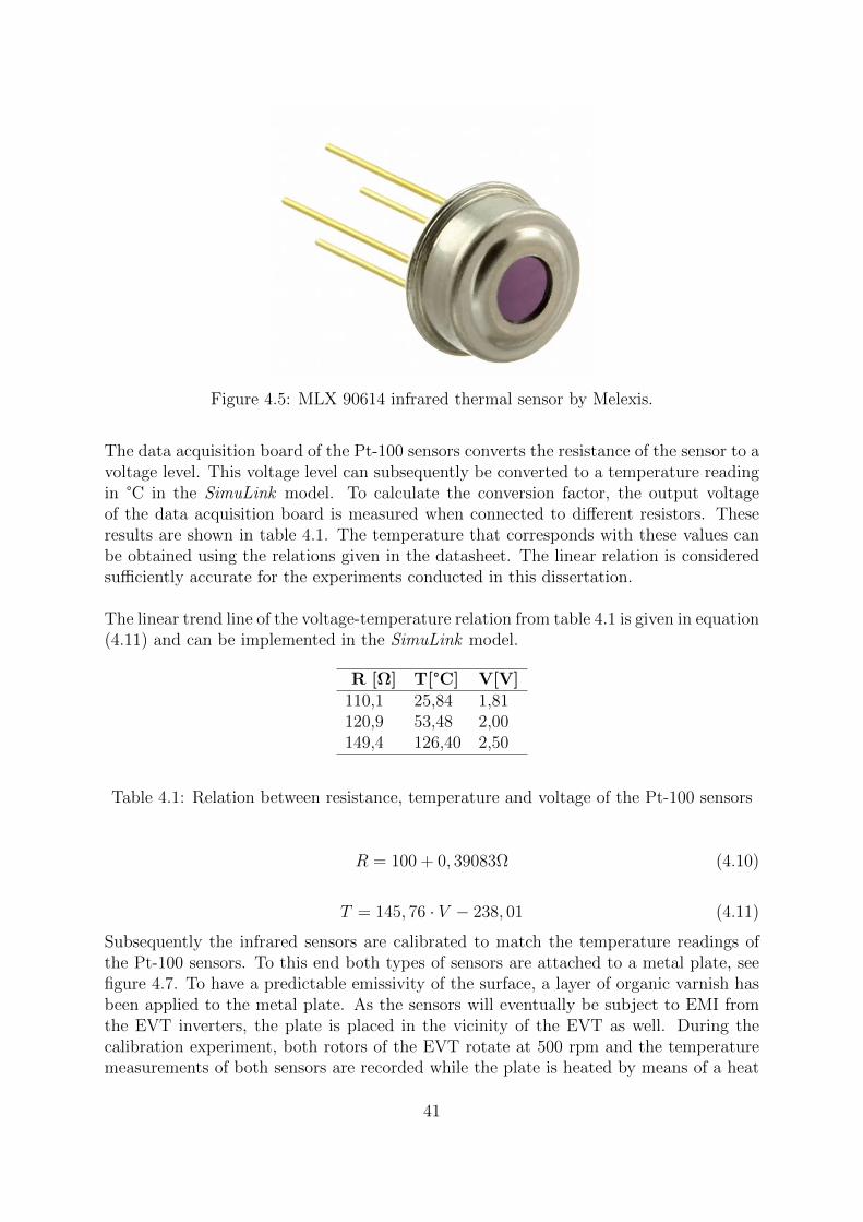
Figure 4.5: MLX 90614 infrared thermal sensor by Melexis.

The data acquisition board of the Pt-100 sensors converts the resistance of the sensor to avoltage level. This voltage level can subsequently be converted to a temperature readingin °C in the SimuLink model. To calculate the conversion factor, the output voltageof the data acquisition board is measured when connected to different resistors. Theseresults are shown in table 4.1. The temperature that corresponds with these values canbe obtained using the relations given in the datasheet. The linear relation is consideredsufficiently accurate for the experiments conducted in this dissertation.

The linear trend line of the voltage-temperature relation from table 4.1 is given in equation(4.11) and can be implemented in the SimuLink model.

R [Ω] T[°C] V[V]110,1 25,84 1,81120,9 53,48 2,00149,4 126,40 2,50

Table 4.1: Relation between resistance, temperature and voltage of the Pt-100 sensors

R = 100 + 0, 39083Ω (4.10)

T = 145, 76 · V − 238, 01 (4.11)

Subsequently the infrared sensors are calibrated to match the temperature readings ofthe Pt-100 sensors. To this end both types of sensors are attached to a metal plate, seefigure 4.7. To have a predictable emissivity of the surface, a layer of organic varnish hasbeen applied to the metal plate. As the sensors will eventually be subject to EMI fromthe EVT inverters, the plate is placed in the vicinity of the EVT as well. During thecalibration experiment, both rotors of the EVT rotate at 500 rpm and the temperaturemeasurements of both sensors are recorded while the plate is heated by means of a heat

41

Figure 4.6: Accuracy of the MLX90614 IR sensor

gun. The results are shown in figure 4.8. There is clearly a steep heating slope anda slow cooling slope. The temperatures of the two sensors show similar trends withthe IR sensor measuring higher temperatures at all times. To calibrate the sensors, thetemperature reading from the IR sensor is plotted against the output of the Pt100 sensorand subsequently linearized for both the heating and the cooling slope, figures 4.8. Thislinearization results in almost the same linear functions. Because the cooling is slower,this slope will be closer to the steady state outputs of both sensors. Therefore thisfunction is used in the SimuLink model, equation (4.12).

T ′IR =TIR − 2.38

1.05(4.12)

Figure 4.7: Set-up for the calibration experiment

42

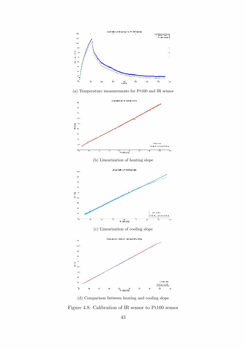
(a) Temperature measurements for Pt100 and IR sensor

(b) Linearization of heating slope

(c) Linearization of cooling slope

(d) Comparison between heating and cooling slope

Figure 4.8: Calibration of IR sensor to Pt100 sensor

43

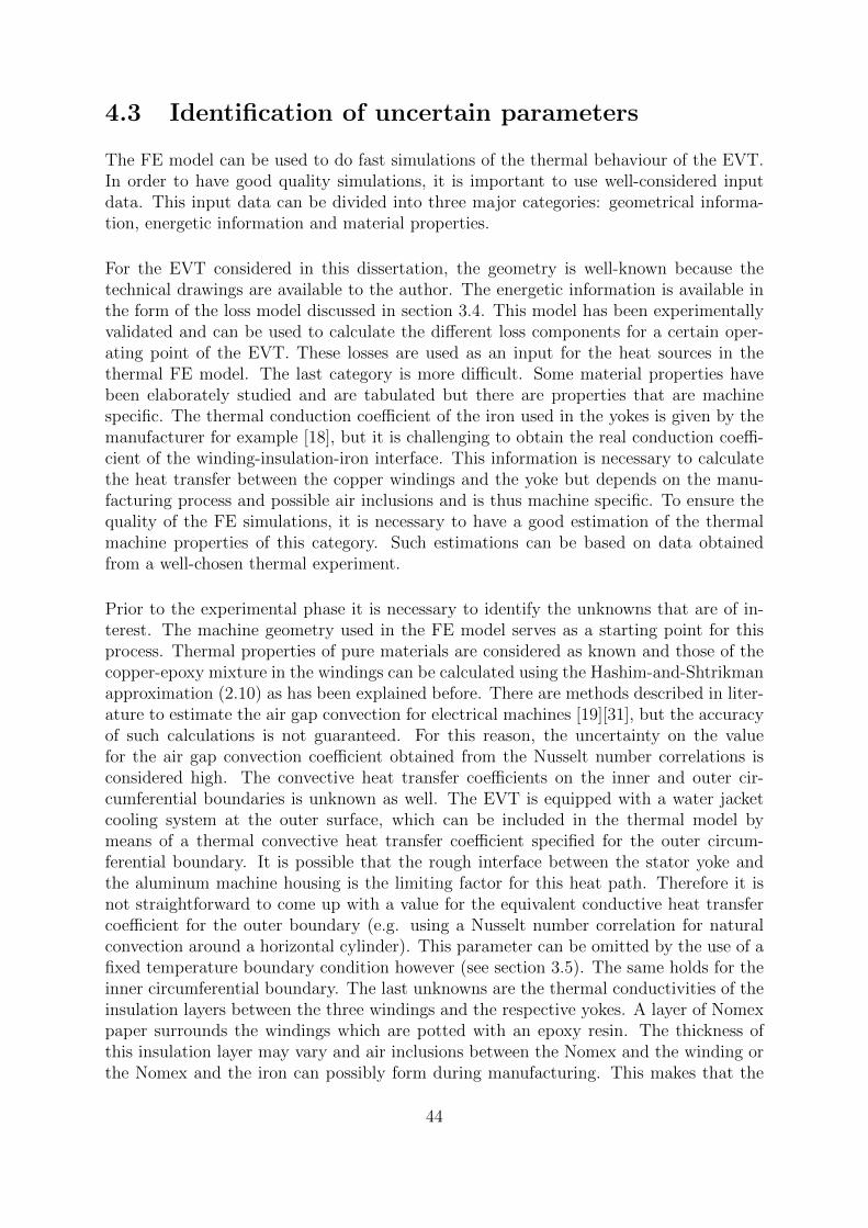
4.3 Identification of uncertain parameters

The FE model can be used to do fast simulations of the thermal behaviour of the EVT.In order to have good quality simulations, it is important to use well-considered inputdata. This input data can be divided into three major categories: geometrical informa-tion, energetic information and material properties.

For the EVT considered in this dissertation, the geometry is well-known because thetechnical drawings are available to the author. The energetic information is available inthe form of the loss model discussed in section 3.4. This model has been experimentallyvalidated and can be used to calculate the different loss components for a certain oper-ating point of the EVT. These losses are used as an input for the heat sources in thethermal FE model. The last category is more difficult. Some material properties havebeen elaborately studied and are tabulated but there are properties that are machinespecific. The thermal conduction coefficient of the iron used in the yokes is given by themanufacturer for example [18], but it is challenging to obtain the real conduction coeffi-cient of the winding-insulation-iron interface. This information is necessary to calculatethe heat transfer between the copper windings and the yoke but depends on the manu-facturing process and possible air inclusions and is thus machine specific. To ensure thequality of the FE simulations, it is necessary to have a good estimation of the thermalmachine properties of this category. Such estimations can be based on data obtainedfrom a well-chosen thermal experiment.

Prior to the experimental phase it is necessary to identify the unknowns that are of in-terest. The machine geometry used in the FE model serves as a starting point for thisprocess. Thermal properties of pure materials are considered as known and those of thecopper-epoxy mixture in the windings can be calculated using the Hashim-and-Shtrikmanapproximation (2.10) as has been explained before. There are methods described in liter-ature to estimate the air gap convection for electrical machines [19][31], but the accuracyof such calculations is not guaranteed. For this reason, the uncertainty on the valuefor the air gap convection coefficient obtained from the Nusselt number correlations isconsidered high. The convective heat transfer coefficients on the inner and outer cir-cumferential boundaries is unknown as well. The EVT is equipped with a water jacketcooling system at the outer surface, which can be included in the thermal model bymeans of a thermal convective heat transfer coefficient specified for the outer circum-ferential boundary. It is possible that the rough interface between the stator yoke andthe aluminum machine housing is the limiting factor for this heat path. Therefore it isnot straightforward to come up with a value for the equivalent conductive heat transfercoefficient for the outer boundary (e.g. using a Nusselt number correlation for naturalconvection around a horizontal cylinder). This parameter can be omitted by the use of afixed temperature boundary condition however (see section 3.5). The same holds for theinner circumferential boundary. The last unknowns are the thermal conductivities of theinsulation layers between the three windings and the respective yokes. A layer of Nomexpaper surrounds the windings which are potted with an epoxy resin. The thickness ofthis insulation layer may vary and air inclusions between the Nomex and the winding orthe Nomex and the iron can possibly form during manufacturing. This makes that the

44

real, machine specific thermal conductivity of this layer possibly deviates from the valuesgiven in the datasheet of the Nomex paper. The parameters with high uncertainty aresummarized in table 4.2.

Parameter Theoretical valuekins,s 0.139kins,DC 0.139kins,r1 0.139

Table 4.2: Overview of thermal parameters with high uncertainty

Once the parameters of interest are identified, one can think about suitable thermal ex-periments to determine their real values. Ideally, each experiment is set up in such mannerthat there is a single unknown in the system. The (in)dependence of the steady statetemperature distribution on a certain parameter can be checked using the FEM model.Furthermore, it is important that the thermal experiment is designed in such way that itcan be conducted on the set-up available in the lab and that the expected temperaturedependency of the variable of interest is as such that it’s value can be determined withsufficient accuracy. All of this will be discussed in detail for each experiment.

4.3.1 Insulation layer stator winding

To determine the effective thermal conductivity of the insulation layer between the statorwindings and the stator yoke, it is necessary to have a known energy flow across this borderand two points of known temperature. When possible, this type of experiment can beconducted using two temperature sensors: one between the winding and the Nomex paperand another one between the Nomex paper and the yoke [35]. When a known power isapplied in the winding, the effective heat conduction coefficient can be calculated whenthe system reaches steady state:

ke =P

A∆T(4.13)

When an existing electrical machine is used in the experiments however, as is the casehere, it is physically not possible to measure the temperature between Nomex and windingand between Nomex and yoke if no temperature sensors have been inserted in theselocations during the manufacturing process. On the EVT prototype, the temperaturecan be measured with Pt-100 sensors attached to the outside of the stator yoke, to theinside of the machine housing and on stator end winding. A known heat source can beinduced in the windings in the form of copper losses or in the stator yoke in the form ofiron losses. When the measured temperature at the outside of the stator iron is used as afixed boundary condition, two uncertainties remain in the system: the equivalent thermalconductivity of the air gap subdomain and the thermal conductivity of the insulationlayer between the stator winding and the stator yoke. The dependency of the steadystate stator winding temperature on the thermal parameter in the air gap can be studiedusing the simulation software. The mean stator winding temperature for a fixed energyinput and varying thermal conductivity in the air gap is given in table 4.3. Based on these

45

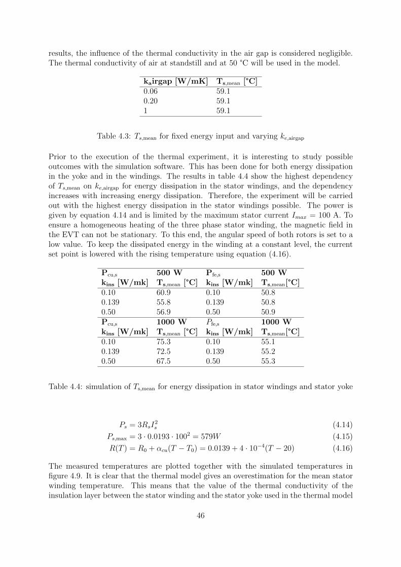
results, the influence of the thermal conductivity in the air gap is considered negligible.The thermal conductivity of air at standstill and at 50 °C will be used in the model.

kairgap [W/mK] Ts,mean [°C]0.06 59.10.20 59.11 59.1

Table 4.3: Ts,mean for fixed energy input and varying ke,airgap

Prior to the execution of the thermal experiment, it is interesting to study possibleoutcomes with the simulation software. This has been done for both energy dissipationin the yoke and in the windings. The results in table 4.4 show the highest dependencyof Ts,mean on ke,airgap for energy dissipation in the stator windings, and the dependencyincreases with increasing energy dissipation. Therefore, the experiment will be carriedout with the highest energy dissipation in the stator windings possible. The power isgiven by equation 4.14 and is limited by the maximum stator current Imax = 100 A. Toensure a homogeneous heating of the three phase stator winding, the magnetic field inthe EVT can not be stationary. To this end, the angular speed of both rotors is set to alow value. To keep the dissipated energy in the winding at a constant level, the currentset point is lowered with the rising temperature using equation (4.16).

Pcu,s 500 W Pfe,s 500 Wkins [W/mk] Ts,mean [°C] kins [W/mk] Ts,mean[°C]0.10 60.9 0.10 50.80.139 55.8 0.139 50.80.50 56.9 0.50 50.9Pcu,s 1000 W Pfe,s 1000 Wkins [W/mk] Ts,mean [°C] kins [W/mk] Ts,mean[°C]0.10 75.3 0.10 55.10.139 72.5 0.139 55.20.50 67.5 0.50 55.3

Table 4.4: simulation of Ts,mean for energy dissipation in stator windings and stator yoke

Ps = 3RsI2s (4.14)

Ps,max = 3 · 0.0193 · 1002 = 579W (4.15)

R(T ) = R0 + αcu(T − T0) = 0.0139 + 4 · 10−4(T − 20) (4.16)

The measured temperatures are plotted together with the simulated temperatures infigure 4.9. It is clear that the thermal model gives an overestimation for the mean statorwinding temperature. This means that the value of the thermal conductivity of theinsulation layer between the stator winding and the stator yoke used in the thermal model

46

Figure 4.9: Simulation compared to experimental values for P,cu = 193W and N1 = N2 =8 rpm

is too low. In order to increase this value in a substantiated way, the composition of thewinding region is examined in more detail. The winding region is depicted in the sketch offigure 4.10. Region A represents the real winding while region B gives an illustration of theapplied homogenization in the winding. The application of a homogenization techniquefor the winding amalgam has as a consequence that the conductors are modelled ascopper cylinders within a layer of epoxy resin of constant thickness. Thus, all conductorsare modelled as completely surrounded by a homogeneous layer of epoxy resin. As isshown in region A of the figure however, it is possible that some of the conductors in thewinding are in direct contact with the Nomex insulation layer. Due to the absence ofthe epoxy layer between the copper conductor and the Nomex insulation layer, and theexcellent thermal conductivity of the copper in the longitudinal direction, this discrepancybetween the model and the physical winding can possibly result in an underestimation ofthe thermal conductivity of the insulation layer surrounding the winding amalgam. Toinclude this observation in the thermal model, the thermal conductivity of the insulationlayer is adapted by excluding the thermal resistance of the layer of epoxy using equations(4.17) to (4.24), see figure 4.11.

47

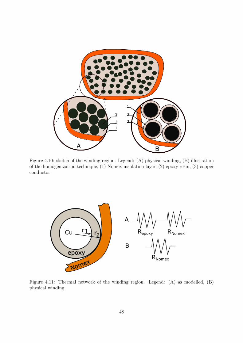
Figure 4.10: sketch of the winding region. Legend: (A) physical winding, (B) illustrationof the homogenization technique, (1) Nomex insulation layer, (2) epoxy resin, (3) copperconductor

Figure 4.11: Thermal network of the winding region. Legend: (A) as modelled, (B)physical winding

48

Figure 4.12: Comparison between simulated and experimental data with the adaptedvalue for knomex. Ps,cu=193 W and N1 = N2 = 8 rpm

Ac =AslotNc

(4.17)

Acu = FF · Ac = πr21 (4.18)

Aepoxy = (1− FF )Ac = π(r22 − r2

1) (4.19)

r1 =

√FF Acπ

(4.20)

r2 =

√(1− FF )Ac

π+ r2

1 (4.21)

Rmodel = kepoxy(r2 − r1) + knomex lnomex (4.22)

Rphysical = ke lnomex (4.23)

Rphysical = Rmodel −→ ke =knomex lnomex + kepoxy (r2 − r1)

lnomex(4.24)

For the stator winding, this corresponds with an increase of the thermal conductivityfor the insulation layer of 0.139 W/mK to 0.53 W/mK. The resulting mean windingtemperature is given in figure 4.12, where it can be seen that increase of the thermalconductivity of the insulation layer results in an improved prediction of the steady statetemperature by the 2D FEM thermal model. The error on the steady value of the meanstator winding temperature is in the order of 0.8 °C, which is within the tolerance limitsof the Pt-100 sensors. Consequently, the adapted value for the thermal conductivity willbe used in the thermal model.

49

Chapter 5

Conclusion

The scientific objective of this work was the development of thermal modelling tools foran EVT with hybrid excitation. These tools can be used in the design process of EVTsystems which are e.g. intended for use in hybrid vehicle applications. In order to op-erate these electrical machines in wide power and torque ranges, it is necessary to havea thorough understanding of the heat generation and heat transfer processes within thesystem to keep the maximum temperatures between the safety limits at all times.

Prior to developing a thermal model for the EVT under consideration, the basic heattransfer mechanisms in electrical machines have been considered. Different thermal mod-elling techniques have been studied in literature as well as the thermal properties ofimportant components of electrical machines. Subsequently a thermal model for theprototype EVT has been developed using the technical drawings of the EVT, thermalmaterial data provided by suppliers or literature and the theoretical approaches from theliterature study applied to the EVT. As this work will be part of a larger frameworkof design tools for the EVT with hybrid excitation, the compatibility with previouslydeveloped electromagnetic models has been a decisive factor for the choice of thermalmodelling approach. For this reason, it has been decided to develop a two-dimensionalFEM thermal model with the software packages Comsol Multiphysics and Matlab.

Once the thermal model for the EVT prototype had been established, it was possibleto predict the temperature distribution within the machine for a given operating point(torque and speed of inner and outer rotor). It is argued in this work that the results ofa thermal model that has been developed using only theoretical approaches and generalmaterial properties can not be regarded as a valuable and reliable output for a designtool. To verify the accuracy of the model’s output, thermal experiments have been con-ducted on the EVT test set-up in EELAB. To this end, both contact and non-contactthermal sensors have been attached to the EVT prototype on reachable and strategicallychosen locations. The thermal experiments have been designed in such way that the ob-tained data could be used to tune the most uncertain parameters in the model. When thethermal experiments showed a discrepancy between the simulated and the actual thermalbehaviour of the machine, it has been tried to reveal the underlying shortcomings in thethermal model and to adapt the concerned parameters in a substantiated manner.

50

The resulting thermal model is can be used to predict the thermal temperature distribu-tion within the prototype EVT depending on the operating point of the machine both forsteady state conditions as well as for transient analysis. The model has been validated bymeans of thermal experiments in which losses have been dissipated in the stator or innerrotor windings and with varying rotational speeds for both rotors. The results show agood agreement between the experimental data and the simulations.

The thermal model as it has been described in tis work is limited in different aspects aswell: first, only heat transfer in the transversal cross section of the EVT has been con-sidered, and second, the model uses fixed temperature boundary conditions on both theinner and outer circumferential boundaries of the geometry. The first limitation inhibitsthe modelling of heat fluxes in the axial direction and assumes a constant temperature inthis direction. When one would want to model more complex heat transfer phenomenasuch as e.g. the end winding cooling in more detail, the use of a three-dimensional thermalmodel may be necessary. The second limitations emerges as soon as it is tried to use thethermal model to simulate the thermal behaviour of the prototype EVT in an operatingpoint other than those of the thermal experiments: the fixed temperatures for the circum-ferential boundary conditions are now unknown, as there is no empirical data available.To overcome this problem, an convective heat transfer coefficient has to be specified forboth boundaries. To this end, the empirical data that has been accumulated during thethermal experiments conducted for this word, could be used together with the simulationsoftware to calculate the thermal convective heat transfer coefficients for both boundaries.

51

Bibliography

[1] David A. Howey, Peter R.N. Childs and Andrew S. Holmes. ‘Air-Gap Convectionin Rotating Electrical Machines’. In: IEEE Transactions on Industrial Electronics59.3 (Mar. 2012), pp. 1367–1375.

[2] Aluminum 7075 Alloy (UNS A97075). url: https://www.azom.com/article.aspx?ArticleID=6652. Accessed: 2019-10-03.

[3] ALuminum 7075-T6; 7075-T651. url: http://asm.matweb.com/search/SpecificMaterial.asp?bassnum=MA7075T6. Accessed: 2019-09-03.

[4] S. Ayat et al. ‘Estimation of equivalent thermal conductivity for impregnated elec-trical windings formed from profiled rectangular conductors’. In: 8th IET Interna-tional Conference on Power Electronics, Machines and Drives (PEMD 2016). Apr.2016, pp. 1–6.

[5] Gaber Beges. ‘Influence of Resistance Method on Motor Winding TemperatureRise Measurement’. In: International Journal of Thermophysics 32 (Dec. 2011).doi: 10.1007/s10765-011-1121-9.

[6] M. Bouafia, Y. Bertin and J. B. Saulnier. ‘Estimation of Equivalent Thermal Para-meters of Impregnated Electrical Windings’. In: International Journal on Heat andMass Transfer 41.10 (1998), pp. 1279–1291.

[7] J. Driesen, R. J. M. Belmans and K. Hameyer. ‘Finite-element modeling of thermalcontact resistances and insulation layers in electrical machines’. In: IEEE Transac-tions on Industry Applications 37.1 (Jan. 2001), pp. 15–20.

[8] Joachim Druant. ‘Modeling and Control of an Electrical Variable Transmission withHybrid Excitation’. PhD thesis. Ghent University, 2018.

[9] J. Druant et al. ‘Dual rotor electrical variable transmission for hybrid vehicles:Performance analysis with focus on losses over a driving cycle’. In: May 2017, pp. 1–6.

[10] DuPont. DuPont Nomex 410 Technical Data Sheet. 2016.

[11] electrical variable transmission homepage. url: http://electricvariabletransmission.com. Accessed: 2019-04-20.

[12] Measurement Specialties Inc. Pt temperature sensor - PTF family. Oct. 2015.

[13] David James Powell. ‘Modelling of high power density electrical machines for aerospace’.PhD thesis. University of Sheffield, 2003.

52

[14] J.Druant et al. ‘Benchmarking the permanent magnet electrical variable transmis-sion against the half toroidal continuously variable transmission’. In: Mechanismand Machine Theory 113 (July 2017), pp. 141–157.

[15] J.Druant et al. ‘Efficiency of a CVT-Operated EVT Experimentally EvaluatedAgainst Half-Toroidal and Push-Belt CVTs’. In: IEEE Transactions on IndustrialElectronics 65.4 (Apr. 2018), pp. 3095–3103.

[16] Damian Kowal. ‘Methodology to Evaluate the Influence of Electrical Steel Prop-erties on the Design of Wind Turbine Generators’. PhD thesis. Ghent University,2013.

[17] Maunu Kuosa, Petri Sallinen and Jaakko Larjola. ‘Numerical and experimentalmodelling of gas flow and heat transfer in the air gap of an electric machine’. In:Journal of Thermal Science 13 (Aug. 2004), pp. 264–278.

[18] Cogent Power Ltd. Electrical Steel Thin Non Oriented.

[19] P.H. Mellor, D. Roberts and D.R. Turner. ‘Lumped parameter thermal model forelectrical machines of TEFC design’. In: IEE Proceedings B - Electric Power Ap-plications 138.5 (Sept. 1991), pp. 205–218.

[20] Janne Nerg. ‘Thermal Modeling of a High-Speed Solid-Rotor Induction Motor’.In: Proceedings of the 5th WSEAS International Conference on Applications ofElectrical Engineering. (Prague, Czech Republic). Prague, 2006, pp. 90–95.

[21] Janne Nerg, Marko Rilla and J Pyrhonen. ‘Thermal Analysis of Radial-Flux Elec-trical Machines With a High Power Density’. In: Industrial Electronics, IEEE Trans-actions on 55 (Nov. 2008), pp. 3543–3554.

[22] Melexis NV. MLX90614 family Single and Dual Zone Infra Red Thermometer inTO-39 Data Sheet. June 2015.

[23] Polyaramid Polymetaphenylene Isopthalamide (Nomex) Properties and ApplicationsSupplier Data by Goodfellow. url: https://www.azom.com/article.aspx?

ArticleID=1994. Accessed: 2019-09-03.

[24] J Pyrhonen, Tapani Jokinen and Valeria Hrabovcova. Design of Rotating ElectricalMachines. Dec. 2008.

[25] J. R. Welty, G. L. Rorrer and D. G. Foster. ‘Fundamentals of Momentum, Heatand Mass Transfer’. In: John Wiley & Sons, 2015. Chap. 14.

[26] H Shimoji, Takashi Todaka and Masato Enokizono. ‘Core loss distribution measure-ment of electrical steel sheets using a thermographic camera’. In: Przeglad Elektro-techniczny 87 (Jan. 2011), pp. 65–68.

[27] L. Siesing, A. Reinap and M. Andersson. ‘Thermal properties on high fill factorelectrical windings: Infiltrated vs non infiltrated’. In: 2014 International Conferenceon Electrical Machines (ICEM). Sept. 2014, pp. 2218–2223.

[28] D.A. Simmers and J.E.R. Coney. ‘A Reynolds Analogy for the Heat Transfer Char-acteristics of Combined Taylor Vortex and Axial Flow’. In: International Journalof Heat and Mass Transfer - INT J HEAT MASS TRANSFER 22 (May 1979),pp. 679–689.

53

[29] N. Simpson, R. Wrobel and P. H. Mellor. ‘Estimation of Equivalent Thermal Para-meters of Impregnated Electrical Windings’. In: IEEE Transactions on IndustryApplications 49.6 (Nov. 2013), pp. 2505–2515.

[30] Dave Staton, Aldo Boglietti and Andrea Cavagnino. ‘Solving the More DifficultAspects of Electric Motor Thermal Analysis’. In: IEEE Transactions on EnergyConversion 20.3 (Aug. 2005), pp. 620–628.

[31] X. Sun and M. Cheng. ‘Thermal Analysis and Cooling System Design of DualMechanical Port Machine for Wind Power Application’. In: IEEE Transactions onIndustrial Electronics 60.5 (May 2013), pp. 1724–1733.

[32] O. J. Tassicker. ‘Measurement of winding temperatures by change of resistance’. In:Proceedings of the Institution of Electrical Engineers 111.8 (Aug. 1964), pp. 1454–1460.

[33] Geoffrey Ingram Taylor. ‘Stability of a Viscous Liquid contained between Two Ro-tating Cylinders’. In: Philosophical Transactions of the Royal Society of London102 (718 Feb. 1923), pp. 289–343. Series A: Containing Papers of a Mathematicalor Physical Character.

[34] Robert Wolf. Physical Properties of Permanent Magnet Materials. url: https:

//www.allianceorg.com/pdfs/PhysicalPropertiesofMagnets.pdf. Accessed:2019-10-03.

[35] Anna Yarantseva. Improvement of the thermal model of an electric machine usinginverse modeling techniques. 2017.

[36] X. Zhang, T. Dong and F. Zhou. ‘Equivalent Thermal Conductivity Estimation forCompact Electromagnetic Windings’. In: IEEE Transactions on Industrial Elec-tronics 66.8 (Aug. 2019), pp. 6210–6219.

[37] P. Zheng et al. ‘Research on the Cooling System of a 4QT Prototype Machine Usedfor HEV’. In: IEEE Transactions on Energy Conversion 23.1 (Mar. 2008), pp. 61–67.

54