Thermal Analysis of a Road on Permafrost

Source: http://simmakers.com/road-on-permafrost/

(Keywords: thermal analysis of a road on permafrost, thermal analysis of a road, simulation of a road in permafrost

area, thermal analysis of roadbed, thermal analysis of road surface)

Road maintenance in permafrost areas is connected with the problem of ensuring soil stability. Roadbed deformations are the result of settlement and heave due to the respective thawing and freezing of underlying moist permafrost soils. These processes cause large amounts of damage on road surfaces.

It is therefore important to pay particular attention to the thermal analysis of soil bases and roadbeds at the design stage to determine the road characteristics such as embankment height, thermal insulation layer thickness, and so on.

Simple 2D thermal analysis cannot account for the changes in terrain and geological structure of the soil throughout the simulated road segment and proper temperature distribution analysis also requires consideration of the influence of solar radiation, road thermal radiation and convective heat transfer due to groundwater filtration. Thus, valid soil and roadbed temperature forecasts must be based on software that allows you to carry out 3D analyses of soil thermal fields, taking into account the above factors. Frost 3D Universal is the most convenient tool for such purposes. An example 3D road section thermal analysis in Frost 3D Universal For our computation, we model a 1.3 km road section located in the upper horizon of permafrost soil.

The three-dimensional geometry of the geotechnical soil structure is reconstructed using geological data interpolation to form the 3D geometry of the embankment, an insulation layer and concrete slabs; all designed natively in the software with special tools for geometric constructions. The computational domain encompasses an area of 1000x300x90 meters.

3D model of a road and geological structure of the soil in an area with complex terrain

Zoom of the 3D model

Roadway design and soils in a cross-section of the computational domain

Boundary conditions are set on the borders of the 3D geometry and the conditions regarding heat exchange with the environment are defined.

The boundary conditions on the 3D hydrogeological model of the road section

In order to consider convective heat exchange with the atmosphere, third-type boundary conditions at the soil/road boundary are set. Air temperature (Tв) is set as a periodic dependency on time over an interval of 1 year:

Month I II III IV V VI VII VIII IX X XI XII

Air temperature, oC -26.4 -26.4 -19.2 -10.3 -2.6 8.4 15.4 11.3 5.2 -6.3 -18.2 -24

The software bases convective heat transfer coefficient (αв) calculations on average wind speeds, which in our example are given in the following table:

Month I II III IV V VI VII VIII IX X XI XII

Wind speed, m/s 2.3 2.3 2.6 3.2 3.2 3.4 3.1 2.6 2.7 2.8 2.4 2.4

To account for the influence of snow cover on heat transfer from soil to the atmosphere, the following snow cover thickness dynamics are set:

Month I II III IV V VI VII VIII IX X XI XII

Snow cover thickness, m 0.47 0.49 0.51 0.47 0.16 0 0 0 0 0.18 0.25 0.38

The calculation assumes that there is no snow cover on the road surface. To consider heating by solar radiation, the following radiation increment is set:

Month I II III IV V VI VII VIII IX X XI XII

Solar radiation, W/m2 1.9 21.2 84.1 157.8 247.7 310.6 296.3 205.6 121.9 39.4 9.3 1.9

For soil, albedo A is assumed to be 0.75; for a reinforced concrete slab, A = 0.2. Surface infrared radiation is factored in via the Stefan – Boltzmann law, with the coefficient of surface emissivity ε taken as 0.9, and the fraction of surface infrared radiation reflected by the atmosphere back to the Earth’s surface, p = 0.9. On the lower boundary, the first-type boundary condition is set: the temperature of the permafrost soil, which is equal to -1.5 oC.

On the lateral boundary of the computational domain, heat flow is equal to zero.

For construction materials (reinforced concrete slab and «penoplex» insulation material), the following thermophysical properties are set:

Parameters

Material short text

Reinforced concrete

slab

Heat insulation

Volumetric heat capacity of material, kJ/(m3∙оС) 2500 62.1

Heat conductivity, W/(m∙оС) 1.5 0.031

Total gravimetric moisture, % 0.0001 0

Density, Kg/m3 2500 45

Phase transition temperature, оС 0 0

Filtration coefficient, µm/s 0.001 0.0000001

Thermophysical properties of some geological layers:

Parameters

Material short text

Embankment Layer 1 Layer 2 Layer 4 Layer

11

Layer

14

Volumetric heat capacity of

thawed ground, kJ/(m3∙оС)

2480 4000 3170 2310 2390 2160

Volumetric heat capacity of

frozen ground, kJ/(m3∙оС)

1890 2310 2410 2140 2080 1800

Heat conductivity of thawed

ground, W/(m∙оС)

1.57 0.81 1.57 1.62 2.0 1.54

Heat conductivity of frozen

ground, W/(m∙оС)

1.86 1.34 1.8 1.74 2.2 1.62

Total gravimetric soil moisture, % 0.2 3.47 0.29 0.18 0.21 0.21

Density of dry soil, Kg/m3 1400 80 1450 1710 1630 1550

Phase transition temperature, оС 0 0 -0.31 -0.38 -0.32 0

Filtration coefficient, µm/s 0.01 0.01 0.01 10 10 10

The dependence of unfrozen water content on temperature is given for each soil type in compliance with SNIP 2.02.04-88 «Bases and Foundations on Permafrost Soils». To solve the heat-filtration equation numerically, the 3D geometry is discretized on the computational mesh consisting of 45.27 million nodes.

3D model computational mesh of the road on permafrost

Computational mesh with decorations of trees and houses

Soil thermal regime forecast can be developed in Frost 3D Universal for any simulation period. Let’s conduct the forecast of soil temperature regime and roadbed for a 3-year period.

As a result of the model computation, we obtain the temperature distribution over different points in time.

The temperature distribution (oC) in the second layer of the ground in the winter after 2.5 years. Top

layer of soil (Layer 1) is disabled

The temperature distribution in the second layer of the ground in summer after 3 years

The temperature distribution on the surface of the ground and the road in the summer after 3 years

The analysis of temperature field dynamics may be performed in a cross-section of the computational domain. The heat distribution in the cross-section may be performed in the form of isolines in addition to color filling. Asymmetrical distribution of temperature isolines is caused by convective heat transfer due to filtration.

The temperature distribution in the cross section of computational domain (winter after 2 years)

The temperature distribution in the form of isolines in the computational domain cross section (winter

after 2 years)

The temperature distribution in the summer after 2 years in the cross section of the computational

domain

The next figure shows that ground located directly beneath the roadbed is thawing up to the embankment basement (see isoline 0 oC position).

The temperature distribution in the cross section of the computational domain in isolines (summer

after 2 years)

A more accurate analysis of the soil thaw depth can be performed in the unfrozen water content view in the program postprocessor.

Relative unfrozen water content distribution (ratio of the unfrozen water content to the total

gravimetric soil moisture: Ww/Wtot) during summer after 2 years

Since the value of the total gravimetric soil moisture (Wtot), is known for each soil type, in order to more accurately represent fully thawed sections, the resulting distribution of unfrozen water content is derived as the ratio of unfrozen water to the total gravimetric soil moisture: Ww/ Wtot(for thawing soil, the unfrozen water content Ww is almost equal to the total gravimetric soil moisture Wtot). The unfrozen water content distribution is hence expressed in the range from zero to one, where one represents fully thawed soil as the unfrozen water content is equal to total gravimetric soil moisture. When soil temperatures is below the initial temperature of the phase transition, the value of the unfrozen water content decreases, and the ratio Ww/Wtot tends towards zero. However, according to the dependence of unfrozen water content on temperature established by SNIP 2.02.04-88 «Bases and Foundations on Permafrost Soils», only sand can have zero unfrozen water when temperatures are below zero degrees Celsius. For other soils at negative temperatures, there is always some

nonzero quantity of unfrozen water. Distribution analysis of the relative unfrozen water content is more conveniently performed on the cross-section of the computational domain.

Relative unfrozen water content distribution after 2 years in summer (computational domain cross

section)

In Frost 3D Universal, the groundwater flow process is simulated based on the Darcy differential equation. For groundwater filtration simulation, the corresponding hydraulic head levels (from 40 to 100 m above sea level) are specified on the side boundaries of the computational domain. For a «headless» ground layer, the value of the hydraulic head is equal to the groundwater level. When considering seasonal changes in groundwater filtration, the value of the hydraulic head on the boundaries is set as a time dependency (e.g., a specific value for each month).

The resulting groundwater filtration velocity simulations in winter and summer in the x-axis direction are shown below.

Filtration velocity along x-axis (micrometers per second) in winter after 2 years

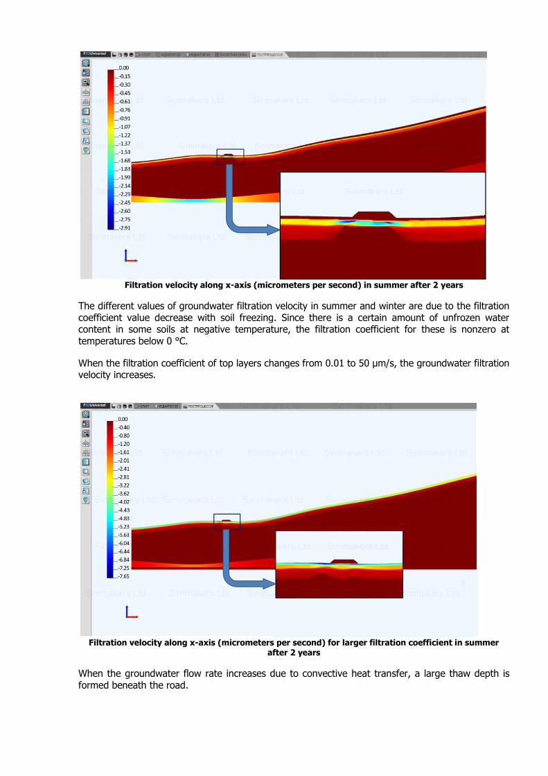
Filtration velocity along x-axis (micrometers per second) in summer after 2 years

The different values of groundwater filtration velocity in summer and winter are due to the filtration coefficient value decrease with soil freezing. Since there is a certain amount of unfrozen water content in some soils at negative temperature, the filtration coefficient for these is nonzero at temperatures below 0 °C.

When the filtration coefficient of top layers changes from 0.01 to 50 µm/s, the groundwater filtration velocity increases.

Filtration velocity along x-axis (micrometers per second) for larger filtration coefficient in summer

after 2 years

When the groundwater flow rate increases due to convective heat transfer, a large thaw depth is formed beneath the road.

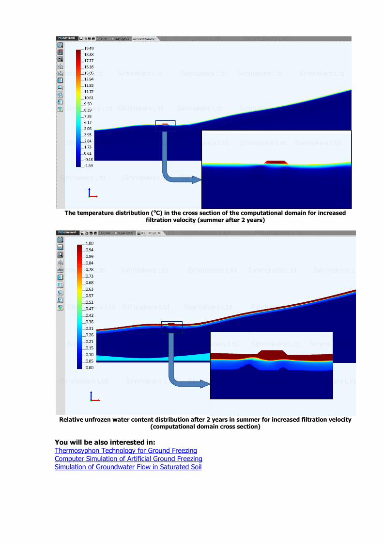
The temperature distribution (oC) in the cross section of the computational domain for increased

filtration velocity (summer after 2 years)

Relative unfrozen water content distribution after 2 years in summer for increased filtration velocity

(computational domain cross section)

You will be also interested in: Thermosyphon Technology for Ground Freezing Computer Simulation of Artificial Ground Freezing Simulation of Groundwater Flow in Saturated Soil