Theory of the Earth Don L. Anderson Chapter 13. Heterogeneity of the Mantle Boston: Blackwell Scientific Publications, c1989 Copyright transferred to the author September 2, 1998. You are granted permission for individual, educational, research and noncommercial reproduction, distribution, display and performance of this work in any format. Recommended citation: Anderson, Don L. Theory of the Earth. Boston: Blackwell Scientific Publications, 1989. http://resolver.caltech.edu/CaltechBOOK:1989.001 A scanned image of the entire book may be found at the following persistent URL: http://resolver.caltech.edu/CaltechBook:1989.001 Abstract: We must now admit that the Earth is not like an onion. The lateral variations of seismic velocity and density are as important as the radial variations. The shape of the Earth tells us this directly but provides little depth resolution. The long-wavelength geoid tells us that lateral density variations extend to great depth. Lateral variations in the mantle affect the orientation of Earth in space and convection in the core; this property of the Earth is known as asphericity. In the following chapters we further admit that the Earth is not elastic or isotropic.

Hetero

"You all do know this mantle."

-SHAKESPEARE, JULIUS CAESAR

W e must now admit that the Earth is not like an onion. The lateral variations of seismic velocity and den-

sity are as important as the radial variations. The shape of the Earth tells us this directly but provides little depth reso- lution. The long-wavelength geoid tells us that lateral den- sity variations extend to great depth. Lateral variations in the mantle affect the orientation of Earth in space and con- vection in the core; this property of the Earth is known as asphericity. In the following chapters we further admit that the Earth is not elastic or isotropic.

UPPER-MANTLE HETEROGENEITY FROM SURFACE-WAVE VELOCITIES

The most complete maps of seismic heterogeneity of the upper mantle are obtained from surface waves. By studying the velocities of Love and Rayleigh waves, of different pe- riods, over many great circles, small arcs, and long arcs, it is possible to reconstruct both the radial and lateral velocity variations. Although global coverage is possible, the limi- tations imposed by the locations of long-period seismic sta- tions and of earthquakes limit the spatial resolution. Fea- tures having half-wavelengths of about 2000 km, as a global average, can be resolved with presently available data. The raw data consist of average group and/or phase velocity over many arcs. These averages can be converted to images using techniques similar to medical tomography. Body waves have better resolution, but coverage, particularly for the upper mantle, is poor.

Even the early surface-wave studies indicated that the upper mantle was extremely inhomogeneous. Shield paths

were fast, oceanic paths were slow, and tectonic regions were also slow (Toksoz and Anderson, 1966; Anderson, 1967). The most pronounced differences are in the upper 200 km, but substantial differences between regions extend to about 400 krn. A high-velocity region was inferred to extend to depths of 120- 150 km under stable continental shields. This thick LID, or seismic lithosphere, probably represents the thickness of the plate. Body-wave results also give a shield LID thickness of about 150 km. On average, the shield mantle is also faster than average oceanic or tec- tonic mantle down to 400 km, but the differences below 200 km are much less than above this depth. Some shield- bearing continents have overriden oceanic lithosphere in the past 50-100 million years, and others were bordered by subduction zones prior to the breakup of Pangaea. Old oce- anic lithosphere has a long thermal time constant and serves to cool off adjacent mantle. Below 200 km the regions of higher than average mantle velocity may represent the cool- ing effect of overriden oceanic lithosphere andlor the ab- sence of a partial melt phase. The rapid decrease in velocity under shields below about 150 km suggests that this is the depth of decoupling. The suggestion that continental roots extend deeper than 400 km (Jordan, 1975) rather than the 150-200 km of earlier studies was based on the low-reso- lution ScS phase rather than the higher resolution P-waves and surface waves (Jordan, 1975; Jordan and Sipkin, 1976).

There are two basic approaches for interpreting global surface-wave data. The regionalized approach introduced by Anderson (1967) and Toksoz and Anderson (1966) di- vides the Earth into tectonic provinces and solves for the velocity of each. Applications of this technique yielded fast shield velocities at short periods or shallow depths but showed that convergence regions were faster at long pe- riods, or greater depth, suggesting that cold subducted ma-

terial was being sampled (Nakanishi and Anderson, 1983, 1984a,b). Convergence regions, on average, are slow at short periods, due to high temperatures and melting at shal- low mantle depths. The regionalization approach is neces- sary when the data are limited or when only complete great- circle data are available. In the latter case the velocity anomalies cannot be well isolated.

If short-arc and long-arc data are available, a complete spherical harmonic expansion can be performed with no as- sumptions required about tectonic regionalizations. Studies of this type have been reported by Nakanishi and Anderson (1983, 1984a,b), Tanimoto and Anderson (1984, 1985) and Woodhouse and Dziewonski (1984). If only complete great- circle data, or free-oscillation data, are available, then only the even-order harmonics can be determined.

In the regionalized models it is assumed that all re- gions of a given tectonic classification have the same ve- locity. This is clearly oversimplified. It is useful, however, to have such maps in order to find anomalous regions. In fact, all shields are not the same, and velocity does not in- crease monotonically with age with the ocean. The region around Hawaii, for example, is faster than equivalent age ocean elsewhere at shallow depth and slower at greater depth. There is also a slow patch in the south-central Pa- cific. The differences between Love wave and Rayleigh wave maps are primarily due to differences in penetration depth and anisotropy between vertical and horizontal S- waves. The early surface-wave results showed that the shal- low mantle was slow, and presumably hot, under young oceans, tectonic regions and subduction zones. Most of the slow regions are in geoid highs. There is a good correspon- dence of surface-wave velocity maps with heat-flow maps but generally poor correlation with the geoid. The geoid, apparently, has little sensitivity to upper-mantle density variations.

GLOBAL SURFACE- WAVE TOMOGRAPHY

A global view of the lateral variation of seismic velocities in the mantle can now be obtained with surface-wave to- mography. In the regionalization approach one assumes that the velocities of surface waves are linearly dependent on the fraction of time spent in various tectonic provinces. The inverse problem then states that the velocity profile depends only on the tectonic classification. For example, all shields are assumed to be identical at any given depth. This as- sumption appears to be approximately valid for the shallow structure of the mantle but becomes increasingly tenuous for depths greater than 200 km. However, it probably provides a maximum estimate of the depth of tectonic features, and it also provides a useful standard model with which other kinds of results can be compared.

The second approach subdivides the Earth into cells or blocks or by some smooth function such as spherical har- monics. Nataf and others (1984, 1986) used spherical harmonics for the lateral variation and a series of smooth functions joined at mantle discontinuities for the radial variation. In this approach no a priori tectonic information is built in.

In both of these approaches the number of parameters that one would like to estimate far exceeds the information content (the number of independent data points) of the data. It is therefore necessary to decide which parameters are best resolved by the data, which is the resolution, or averaging length, which parameters to hold constant and how the model should be parameterized (for example as layers or srnooth functions, isotropic or anisotropic). In addition, there are a variety of corrections that might be made (such as crustal thickness, water depth, elevation, ellipticity, at- tenuation). The resulting models are as dependent on these assumptions and corrections as they are on the quality and quantity of the data. This is not unusual in science: Data must always be interpreted in a framework of assumptions, and the data are always, to some extent, incomplete and inaccurate. In the seismological problem the relationship between the solution, or the model, including uncertainties, and the data can be expressed formally. The effects of the assumptions and parameterizations, however, are more ob- scure, but these also influence the solution. The hidden assumptions are the most dangerous. For example, most seismic modeling assumes perfect elasticity, isotropy, geo- metric optics and linearity. To some extent all of these as- sumptions are wrong, and their likely effects must be kept in mind.

Nataf and others (1986) made an attempt to evaluate the resolving power of their global surface-wave dataset and invoked physical a priori constraints in order to reduce the number of independent parameters that needed to be es- timated from the data. For example, the density, com- pressional velocity and shear velocity are independent pa- rameters, but their variation with temperature, pressure and composition show a high degree of correlation; that is, they are coupled parameters. Similarly, the fact that temperature variations in the mantle are not abrupt means that lateral antd radial variations of physical properties will generally be smooth except in the vicinity of phase boundaries, in- cluding partial melting. Changes in the orientation of crys- tals in the mantle will lead to changes in both the shear- wave and compressional velocity anisotropies. These kinds of physical considerations can be used in lieu of the standard seismological assumptions, which are generally made for mathematical convenience rather than physical plausibility.

The studies of Woodhouse and Dziewonski (1984) and Nataf and others (1984, 1986) give upper-mantle models that are based on quite different assumptions and analyti- cal techniques. Woodhouse and Dziewonski inverted for

FIGURE 13-1 Group velocity of 152-s Rayleigh waves (kmls). Tectonic and young oceanic areas are slow (dashed), and continental shields and older oceanic areas are fast. High temperatures and partial melting are responsible for low velocities. These waves are sensitive to the upper several hundred kilometers of the mantle (after Nakanishi and Anderson, 1984a).

shear velocity, keeping the density, compressional velocity and anisotropy fixed. They also used a very smooth radial perturbation function that ignores the presence of mantle discontinuities and tends to smear out anomalies in the vertical direction. They corrected for near-surface effects by assuming a bimodal crustal thickness, continental and oceanic.

Nataf and others corrected for elevation, water depth, shallow-mantle velocities and measured or inferred crustal thickness. They inverted for shear velocity and anisotropy, the dominant parameters, but included physically plausible accompanying changes in density, compressional velocity and anisotropy. Corrections were also made for anelasticity. The radial perturbation functions were allowed to change rapidly across mantle discontinuities, if required by the data. In spite of these differences, the resulting models are remarkably similar above about 300 km. The main differ- ences occur below 400 km and seem to arise from differ- ences in the assumptions and parameterizations (crustal cor- rections, radial smoothing functions) rather than the data. The choice of an a priori radial perturbation function can degrade the vertical resolution intrinsic to the dataset. The solution, in this case, is overdamped or oversmoothed.

Before discussing the inversion results-the earth structures themselves-I will briefly describe the distribu-

tion of Love and Rayleigh wave velocities (Nakanishi and Anderson, 1983, 1984a,b).

Love waves are sensitive to the SH velocity of the shal- low mantle, above about 300 km for the periods considered here. The slowest regions are at plate boundaries, particu- larly triple junctions. Slow velocities extend around the Pa- cific plate and include the East Pacific Rise, western North America, Alaska-Aleutian arcs, Southeast Asia and the Pa- cific-Antarctic Rise. Parts of the Mid-Atlantic Rise and the Indian Ocean Rise are also slow. The Red Sea-Gulf of Aden-East Africa Rift (Afar triple junction) is one of the slowest regions. The upper-mantle velocity anomaly in this slowly spreading region is as pronounced as under the rap- idly spreading East Pacific Rise. Since it also shows up for long-period Rayleigh waves, this is a substantial and deep- seated anomaly. Shields are generally fast, particularly the Brazilian, Australian and South African shields. The fastest oceanic regions are the north-central Pacific, centered near Hawaii, and the eastern Indian Ocean.

Rayleigh waves are sensitive to shallow P-velocities and SV velocity from about 100 to 600 km. The fastest re- gions (see Figure 13-1) are the western Pacific, western Af- rica and the South Atlantic. Western North America, the Red Sea area, Southeast Asia and the North Atlantic are the slowest regions. Slower than average Rayleigh-wave phase

velocities are obtained at long period for the stable conti- nental areas. The velocities in the South Atlantic and the Philippine Sea plate are faster than shields.

Regions of convergence, or descending mantle flow, are relatively fast for long-period Rayleigh waves, particu- larly near New Guinea, Sumatra, the western Pacific and northwestern Pacific. These regions have large positive ge- oid anomalies. Dense, cold material in the upper mantle can explain these results. To explain the surface-wave results, the fast material must be below the depth sampled by 250-s Love waves and 150-s Rayleigh waves, which is about 300 km depth, and must occupy a considerable volume of the upper mantle. Conductive cooling of the oceanic litho- sphere probably extends no deeper than about 150 km. It is doubtful that the subduction of such a thin high-velocity plate could explain these results. Either slabs preferentially subduct in cold regions of the mantle or they pile up in the upper mantle. At shorter periods the velocity of the mantle beneath subduction zones is average or slower than aver- age, presumably reflecting the extensional tectonics and hot shallow mantle under back-arc basins.

A map synthesized from the 1 = 2 coefficients at 250 s is characterized by a broad closed high-velocity re- gion centered in the western Pacific, northeast of New Guinea, and a low-velocity region centered on the East Pa- cific Rise. Because of symmetry the antipodal regions are identical. The 1 = 2 coefficients are just part of the com- plete set that is required to fully describe the Earth's aspher- icity and need no special explanation. The 1 = 2 pattern of the associated density field does have special significance because it is involved in the Chandler wobble, tidal friction, the orientation of the Earth's spin axis and polar wander. Tectonic models based on surface tectonics have a strong 1 = 2 component, because of the ocean-continent configu- ration, the locations of island arcs, and the thermal struc- ture of the seafloor. In particular, the velocity highs en- compass most of the world's old oceanic lithosphere and convergence regions, and the lows include most of the young oceanic lithosphere and many of the world's hot- spots. The correlation between surface-wave velocity and heat flow and tectonics, and between velocity and geoid is relatively high for 1 = 2, particularly at long periods. If the rotation axis of the Earth is controlled by density anomalies in the upper mantle, and if density correlates with velocity, then the pattern would be symmetric about the equator.

The overall pattern of the Love-wave phase velocity variations shows a general correlation with surface tecton- ics. These waves are most sensitive to the SH velocity in the upper 200 to 300 km of the mantle.

The lowest velocity regions are located in regions of extension or active volcanism: the southeastern Pacific, western North America, northeast Africa centered on the Afar region, the central Atlantic, the central Indian Ocean, and the marginal seas in the western Pacific. A high- velocity region is located in the north central Pacific, cen-

tered near the Hawaiian swell. Love-wave velocities are low along parts of the Mid-Atlantic Ridge, especially near the triple junctions in the North and South Atlantic.

High-velocity regions in continents generally coin- cide with Precambrian shields and Phanerozoic platforms (northwestern Eurasia, western and southern parts of Af- rica, eastern parts of North and South America, and Antarc- tica). Tectonically active regions, such as the Middle East centered on the Red Sea, eastern and southern Eurasia, eastern Australia, and western North America are slow, as are island arcs or back-arc basins such as the southern Alaskan margin, the Aleutian, Kurile, Japanese, Izu-Bonin, Mariana, Ryukyu, Philippine, Fiji, Tonga, Kermadec, and New Zealand arcs.

Rayleigh-wave velocity also correlates well with sur- face tectonics, particularly at short periods. The periods generally considered are most sensitive to S V velocity be- tween about 100 and 400-600 km and thus sample deeper than the Love waves.

The slowest regions, for Rayleigh waves, are centered on the Red Sea-Afar region, Kerguelen-Indian Ocean triple junction, western North America centered on the Gulf of California, the northeast Atlantic, and Tasman Sea- New Zealand-Campbell Plateau. The fastest regions are the western Pacific, New Guinea-western Australia-eastern Indian Ocean, west Africa, northern Europe and the South Atlantic.

One difference between Love waves and Rayleigh waves is evident in the island arcs along the northwestern margins of the Pacific Ocean, such as the Aleutian, Kurile, Japanese, Izu-Bonin-Mariana, Ryukyu, and Philippine re- gions. These regions are characterized by high velocity for Rayleigh waves. The difference between Love and Rayleigh wave results is partially explained by the difference in pene- tration depth. The Love-wave results indicate that the shal- low mantle, in the vicinity of island arcs and back-arc ba- sins, is slow. Rayleigh waves sample the fast material that has subducted beneath the island arcs. Because of the large wavelengths, the lateral extent of the fast material must be considerable. Anisotropy may also be involved: In regions of convergence and divergence, the mantle flow can be ex- pected to be generally vertical, whereas in the centers of convection cells, the flow is mainly horizontal. The sense of anisotropy will change at ridges and subduction zones.

For Rayleigh waves the Atlantic Ocean is generally high velocity except for the northern part. The low veloci- ties associated with the midoceanic ridge system, which ap- pear in the Love-wave maps, are not evident in the long- period Rayleigh-wave maps. This may indicate that many ridge segments are passive or that SV exceeds SH in regions of ascending flow.

Maps of surface-wave velocity (Nakanishi and Ander- son, 1983, 1984a,b) provide, perhaps, the most direct dis- play possible of the lateral heterogeneity of the mantle. The phase and group velocities can be obtained with high pre-

cision and with relatively few assumptions. In general, the shorter period waves, which sample only the crust and shallow mantle, correlate well and as expected with sur- face tectonics. The longer period waves, which penetrate into the transition region (400-650 km), correlate less well with surface tectonics. The inversion of these results for Earth structure involves many more assumptions and approximations.

REGIONALIZED INVERSION RESULTS

Figure 13-2 shows vertical shear-velocity profiles, ex- pressed as differences from the average Earth, using the re- gionalization approach (Nataf and others, 1986). Young oceans, region D, have slower than average velocities throughout the upper mantle and are particularly slow be- tween 80 and 200 km, in agreement with the higher reso- lution body-wave studies. Old oceans, region A, are fast throughout the upper mantle. Intermediate-age oceans (B and C) are intermediate in velocity at all depths. Most of the oldest oceans are adjacent to subduction zones, and the subduction of cold material may be partially responsible for the fast velocities at depth. Notice that velocities converge toward 400 km but that differences still remain below this

Velocity variation (kmls) FIGURE 13-2 Variation of the S V velocity with depth for various tectonic provinces. A-D, oceanic age provinces ranging from old, A, to young, D; S, continental shields; M, mountainous areas; T, trench and island-arc regions. These are regionalized results (after Nataf and others, 1986).

depth. The continuity of the low velocities beneath young oceans, which include midocean ridges, suggests that the ultimate source region for MORB is below 400 km. Shields (S) are faster than all other tectonic provinces except old ocean from 100 to 250 km. Below 220 km the velocities under shields decrease, relative to average Earth, and below 400 km shields are among the slowest regions. At all depths beneath shields the velocities can be accounted for by rea- sonable mineralogies and temperatures without any need to invoke partial melting. Trench and marginal sea regions (T), on the other hand, are relatively slow above 200 km, probably indicating the presence of a partial melt, and fast below 400 km, probably indicating the presence of cold subducted lithosphere. The large size of the tectonic regions and the long wavelengths of surface waves require that the anomalous regions at depth are much broader than the sizes of slabs or the active volcanic regions at the surface. This suggests very broad upwellings under young oceans and abundant piling up of slabs under trench and old ocean re- gions. The latter is evidence for layered mantle convection and the cycling of oceanic plates into the transition region.

Shields and young oceans are still evident at 250 km. At 350 km the velocity variations are much suppressed. Be- low 400 km, most of the correlation with surface tectonics has disappeared, in spite of the regionalization, because shields and young oceans are both slow, and trench and old ocean regions are both fast. Most of the oceanic regions have similar velocities at depth. This is a severe test of the continental tectosphere hypothesis of Jordan (19751, de- scribed later in this chapter. Shields do not have higher ve- locities than some other tectonic regions below 250 km and definitely do not have "roots" extending throughout the up- per mantle or even below 400 km. Results for other depths are given by Nataf and others (1984, 1986). In high- resolution body-wave studies, subshield velocities drop rap- idly at 150 km depth, although velocities remain relatively high to about 390 km. These high velocities could represent "roots" physically attached to the shield lithosphere, over- ridden cold oceanic lithosphere or simply "normal" con- vecting mantle weakly coupled to the overlying shield litho- sphere via a boundary layer at 150-200 km depth. The velocities below 200 krn can be explained by an adiabatic temperature gradient and therefore probably represent nor- mal convecting mantle. Therefore, it is the slow mantle un- der ridges and tectonic regions that is anomalous, and, if anything, these are the regions with the roots. If the mantle under shields is convectively stagnant, as implied by the deep tectosphere hypothesis, a high thermal gradient would extend over a large depth interval. This could lead to par- tial melting and a depression of the olivine-spinel phase boundary under shields. I therefore prefer the 150-km-thick plate hypothesis, that is, a correspondence of the thickness of the plate with the seismic high-velocity layer. The slightly higher than average subshield mantle between about 200 km and 350-390 km may be a boundary layer or could

represent colder than average mantle over which the conti- nents have drifted.

SPHERICAL HARMONIC INVERSION RESULTS

An alternative way to analyze the surface-wave data is through a spherical harmonic expansion that ignores the surface tectonics (Nataf and others, 1986). This provides a less biased way to assess the depth extent of tectonic features.

The mantle is assumed to have the same average prop- erties, including anisotropy, as the PREM Earth model given in the Appendix. Perturbations are assumed to be smooth between the discontinuities in PREM (60, 220, 400 and 670 km) and to be loosely coupled across these discon- tinuities. Thus, the radial variation in perturbation can change rapidly at physical discontinuities. Woodhouse and Dziewonski (1984) invoked a smooth radial perturbation

NNAG, vertical shear velocity,

throughout the upper mantle in their inversions. The data set is not yet complete enough to favor one parameterization over another. In the parameterization of Nataf and others (1 984, 1986), the variation across the discontinuities is con- tinuous unless the data require otherwise. In general, the perturbations across discontinuities are highly correlated. In both of these models the character of the perturbations changes at 220 and 400 km. In particular, the amplitudes of the perturbations decrease with depth.

At shallow depths we have little resolution because global maps for short-period surface waves have not yet been prepared. Nevertheless, surface waves sense the shal- low structure, and some information is available. At a depth of 50 km the major tectonic features correlate well with the shear velocity. Shields and old oceans are fast. Young oce- anic regions and tectonic regions are slow. The slowest re- gions are centered near the midocean ridges, some back-arc basins and the Red Sea. The hotspot province in the south Pacific is slow at shallow depths, but the shallow mantle in thle north-central Pacific, including Hawaii, is fast. The shields are particularly fast. At 150 km all the major shield

depth: 250km

FIGURE 13-3 Map of SV velocity at 250 krn depth from sixth-order spherical harmonic representation of Nataf and others (1984). Note the slow regions associated with the midocean ridges. The fastest regions are in the far south Atlantic, some subduction areas and northwest Africa.

areas fall near the centers of high-velocity anomalies, and the ridges are in low-velocity regions. The main differences at this depth, compared to the regionalized models, are the very low velocities in eastern Asia, the Red Sea region, and New Zealand. The central Pacific and the northeastern Ih- dian Ocean are fast. The Arctic Ocean between Canada and Siberia is slow. At 250 km (see Figure 13-3), the shields are less evident than at shallower depths and than in the region- alized model. On the other hand, the areas containing ridges are more pronounced low-velocity regions. The central Pa- cific and the Red Sea are also very slow. The prominent low-velocity region in the central Pacific roughly bounded by Hawaii, Tahiti, Samoa and the Caroline Islands is the Polynesian Anomaly. This feature may be related to the extensive volcanism that occurred in the western Pacific in the Cretaceous when the Pacific plate was over this anomaly. The northern and southern Atlantic are also slow. Northern Europe and Antarctica are mainly fast. The high- est velocity anomalies are in the far south Atlantic, north-

west Africa to southern Europe and the eastern Indian Ocean to southeast Asia and are not confined to the older continental areas. At 340 km (Figure 13-4), most ridges are still evident although the slow region of the eastern Pacific has shifted off the surface expression of the East Pacific Rise. A central Pacific slow-velocity region persists throughout the upper mantle. The shield areas are no longer evident. Some ridges have average or faster than average velocities at this depth, particularly the Australian- Antarctic ridge and the central Atlantic ridge. These ridge segments are in relative geoid lows. This may indicate that parts of the ridge system involve lateral transport at shallow depth. Generally, however, the source for midocean ridges appears to extend below 350 km depth. Below 400 km there is little correlation with surface tectonics, and in many areas the velocity anomalies are of opposite sign from those in the shallow mantle, in agreement with the regionalized results. The net result is that shields, on average, have very high velocities to 150-200 km, and ridges, on average, have low

NNA6, vertical shear velocity, depth: 340 km

Scale : FIGURE 13-4 Map of SV velocity at 340 km depth. A, prominent low-velocity anomaly shows up in the central Pacific (the Polynesian Anomaly). The fast anomalies under eastern Asia, northern Africa and the South Atlantic may represent mantle that has been cooled by subduction.

~ O O 0 0 0 0 o ~ ~ ~ ~ O ~ ~ ~ ~ O O D ~ ~ ~ ~ ~ ~ ~ ~ ~ O ~ ~ ~ ~ ~ ~ ~ ~ . . . . m . o . . 0 0 0 0 0 . . . - . O . . . . . . . . . . . . . . . o o o o . . . . . . . . o 0 0 0 0 . . . . . . . . . . . . . . . a o o . . . . . .

. . . . . . . . . . . . . . . . . . . . . . . . . . . . . . . . . . 00o.........oooo.......- o o o o . . . . o e . . ~ a o o ~ . . . . o . . 0 0 , r . . . . . . . . . . . . . . . . . . . . . . . . . . . . .

. . . . . . . . . . . . . . . . . . . . . . . . . . . . . . . . . . . . . . . . . . . . . . . . . . . . n o 0 0 0 . . . . . . . . . . . . . . . . . . . . . . . . . . . . . . . . . . . . . . . . . . . . . . . . . . . . . .

0 0 0 0 ....... a . . . . . . . . . . . . . . . . . 0 . . . . 0 0 0 0 0 . . . . . . . . . . . . . . . . . . . . . . . . . . . . . . . . . . . 0 0 0 0 o . . . . . . . . . . . . . - . 0 0 0 o o . e . . . o o o . . . . . . . . . . . . . . . . . . . . . O o O O O o . . . a . . . . . . . . . . . . . . . . . . . . . . . . . . . . . . . . . . . . . m e . . 0 0 0 o o . . . . . o O O O O O O .

. . . . . m . . . . . 0 0 0 0 . . . . . . . . . . . @ . n - - < - I -l-

FIGURE 13-5 SV velocity from 50 to 550 krn along the great-circle path shown. Cross-sections are shown with two vertical exaggerations. Note the low-velocity regions in the shallow mantle below Mexico, the Afar and south of Australia and the asymmetry of the North Atlantic. Velocity variations are much more extreme at depths less than 250 km than at greater depths. The circles on the map represent hotspots.

velocities to 350-400 km. The Red Sea anomaly appears to extend to 400 km, but the very slow velocities associated with western North America die out by 300 km.

By 400 or 450 km the pattern seen at shallow depths changes dramatically. The mantle beneath most ridges is fast. The Polynesian Anomaly, although shifted, is still present. Eastern North America and/or the western North Atlantic are slow. Most of South America, the South Atlan- tic and Africa are fast. The north-central Pacific is slow. Most hotspots are above faster-than-average parts of the mantle at this depth. The fast regions under the Atlantic, western North America, the western Pacific and south of Australia may be sites of subducted or overriden oceanic

lithosphere. Prominent slow anomalies are under the north- ern East Pacific Rise and in the northwest Indian Ocean. The central Atlantic and the older parts of the Pacific are fast. Most of the large slow anomalies define geoid highs. There is poor overall correlation between velocities in the upper mantle and the geoid because subduction zones in general are associated with geoid highs and regions of fast velocity below 300 km. Hot and slow regions of the upper mantle generate geoid highs because of thermal expansion and uplift of the surface. Cold and fast regions of the mantle (subduction zones) generate geoid highs because the excess mass is held up by increasing intrinsic density or viscosity with depth (that is, it is uncompensated).

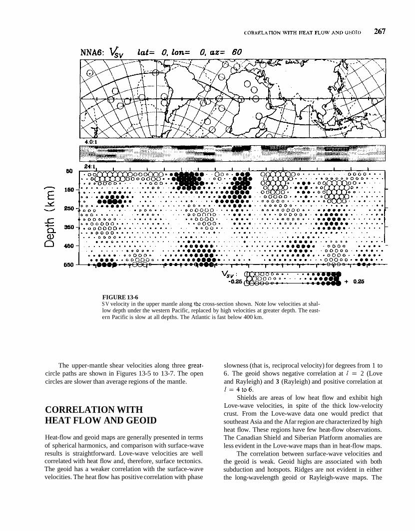
FIGURE 13-6 S V velocity in the upper mantle along the cross-section shown. Note low velocities at shal- low depth under the western Pacific, replaced by high velocities at greater depth. The east- ern Pacific is slow at all depths. The Atlantic is fast below 400 km.

The upper-mantle shear velocities along three great- circle paths are shown in Figures 13-5 to 13-7. The open circles are slower than average regions of the mantle.

CORRELATION WITH HEAT FLOW AND GEOID

Heat-flow and geoid maps are generally presented in terms of spherical harmonics, and comparison with surface-wave results is straightforward. Love-wave velocities are well correlated with heat flow and, therefore, surface tectonics. The geoid has a weaker correlation with the surface-wave velocities. The heat flow has positive correlation with phase

slowness (that is, reciprocal velocity) for degrees from 1 to 6. The geoid shows negative correlation at I = 2 (Love and Rayleigh) and 3 (Rayleigh) and positive correlation at 1 = 4 t o 6 .

Shields are areas of low heat flow and exhibit high Love-wave velocities, in spite of the thick low-velocity crust. From the Love-wave data one would predict that southeast Asia and the Afar region are characterized by high heat flow. These regions have few heat-flow observations. The Canadian Shield and Siberian Platform anomalies are less evident in the Love-wave maps than in heat-flow maps.

The correlation between surface-wave velocities and the geoid is weak. Geoid highs are associated with both subduction and hotspots. Ridges are not evident in either the long-wavelength geoid or Rayleigh-wave maps. The

FIGURE 13-7 Cross-section illustrating the low upper-mantle shear velocities under midocean ridges and western North America. Stable regions are relatively fast in the shallow mantle.

1 = 2 correlation indicates that the long-wavelength part of the geoid has a negative correlation with slowness; that is, I = 2 geoid highs correlate with 1 = 2 velocity highs. For shorter wavelength features the reverse is the case.

Surface-wave studies show (I) low-velocity anomalies centered on southeast Asia, Afar and the Gulf of California, the latter two persisting to long periods thus indicating a deep upper mantle origin; (2) an association of high veloci- ties, at long periods, with the western Pacific subduction zones, indicating a large volume of fast material in the up- per mantle; and (3) high velocities in the South Atlantic that do not have an obvious explanation in terms of pres- ent plate configurations. The South Atlantic may overlie an- cient subducted Pacific Ocean lithosphere.

Regions of generally faster than average velocity occur in the western Pacific, the western part of the African plate, Australia-southern Indian Ocean, part of the south Atlan-

tic, northeastern North America-western North Atlantic, and northern Europe. These are all geoid lows in an 1 =

4-9 expansion of the geoid. Dense regions of the mantle that are in isostatic equi-

librium generate geoid lows (Haxby and Turcotte, 1978; Hager, 1983). High density and high velocity are both con- sist~ent with cold mantle. The above regions may be under- lain by cold subducted material. Geoid highs occur near Tonga-Fiji, the Andes, Borneo, the Red Sea, Alaska, the northern Atlantic, and the southern Indian Ocean. These are generally slow regions of the mantle and are therefore pre- sumably hot. The upward deformation of boundaries coun- teracts the low density associated with the buoyant material, and for uniform viscosity the net result is a geoid high (Hager, 1983). An isostatically compensated column of low-density material also generates a geoid high because of the elevation of the surface.

Correlation coefficients between phase velocity and the geoid show that Love waves generally have a negative correlation (geoid highs correlate with slow velocity) for 1 = 4-6. Rayleigh waves generally correlate well with the geoid only for 1 = 6 and, at some periods, with 1 = 5. The 1 = 6 correlation is particularly strong for both Love waves and Rayleigh waves.

Hager (1983) found an excellent correlation between the observed geoid and the "slab geoid" for 1 = 4, 5, and 7-9 and weak correlation at 1 = 6. There is a high degree of correlation of subduction zones with geoid highs, par- ticularly those centered on Tonga-Fiji, Borneo, Alaska and Peru, and associated lows such as the Nazca plate, the west- ern Pacific, and western Australia. The slab geoid does not explain the geoid lows in Siberia, Canadian shield-western Atlantic, and the South Atlantic or the geoid highs in the south Indian Ocean, the Red Sea, and the North Atlantic. These are high-velocity and low-velocity regions, respec- tively. The slab geoid predicts higher than observed anoma- lies in Tonga-Fiji, Japan and the Kuriles. The slab-geoid correlation can be understood in terms of a large amount of dynamically supported dense material either in the upper mantle or in both the upper and lower mantles in the vicinity of active subduction zones (Hager, 1983). The surface wave-geoid correlation, which apparently explains the missing 1 = 6 component of the slab geoid, however, must be due to an anomalous mass distribution in the shallow mantle.

These results suggest that features of the geoid having wavelengths of about 4000 to 10,000 krn are generated in the upper mantle. Geoid anomalies of this wavelength gen- erally have an amplitude of about 20 to 30 m. An isostati- cally compensated density anomaly of 0.5 percent spread over the upper mantle would give geoid anomalies of this size. It therefore appears that a combination of slabs and broad thermal anomalies in the upper mantle can explain the major features of the 1 = 4-9 geoid. The longer wave- length part of the geoid, 1 = 2 and 3, correlates with seis- mic velocities in the deeper part of the mantle. The shorter wavelength (1 > 9) part of the geoid correlates with topog- raphy. Topography and geoid also correlate moderately well at 1 = 4 and 6, but crustal thickness variations and the distribution of the continents, with shallow compensation, do not explain the magnitude of the effect. Figure 13-8 shows the actual distribution of Love-wave phase velocities and that computed from the geoid assuming a linear rela- tionship between velocity and geoid height. Most subduc- tion regions are slow at short periods, presumably because of the presence of back-arc basins and hot, upwelling ma- terial above the slab.

Slabs are colder than normal mantle and therefore they are denser. Denser minerals also occur in the slab because of temperature-dependent phase changes (Chapter 16). The phase change effect leverages the role of temperature with

FIGURE 13-8 The intermediate wavelength (1 - 6) geoid is controlled by pro- cesses in the upper mantle (slabs, hot asthenosphere). (a) The 1 = 6 component of a global spherical harmonic expansion of Love-wave phase velocities. These are sensitive to shear velocity in the upper several hundred kilometers of the mantle. Note that most shields are fast (gray areas), and oceanic and tectonic re- gions are slow (white areas). Hot regions of the upper mantle, in general, cause geoid highs because of thermal expansion and uplift of the surface and internal boundaries. Tectonic and young oceanic areas are generally elevated over the surrounding terrain. (b) Phase velocity computed from the I = 6 geoid, assuming a linear relationship between geoid height and phase velocity. Note the agreement between these two measures of upper-mantle properties (Tanimoto and Anderson, 1985).

the result that slabs confined to the upper mantle can explain the magnitude of the slab-related geoid.

AZIMUTHAL ANISOTROPY

The velocities of surface waves depend on position and on the direction of travel. If an adequately dense global cov- erage of surface-wave paths is available, then azimuthal an- isotropy as well as lateral heterogeneity can be studied. Pre- liminary maps of azimuthal anisotropy have been prepared by Tanimoto and Anderson (1984, 1985). Regional surface- wave studies also give azimuthal variations (Forsyth, 1975).

HETEROGENEITY OF THE MANTLE

- 2 percent

FIGURE 13-9 Azimuthal variation of phase velocities of 200-s Rayleigh waves (expanded up to 1 = m = 3) (after Tanimoto and Anderson, 1984, 1985).

Azimuthal anisotropy can be caused by oriented crys- tals or a consistent fabric caused by, for example, dikes or convective rolls in the shallow mantle. In either case, the azimuthal variation of seismic-wave velocity is telling us something about convection in the mantle. Since long- period surface waves see beneath the plates, it may be pos- sible to map the direction of flow in the asthenosphere and thus discuss the nature of lithosphere-asthenosphere cou- pling, style of mantle convection and the viscosity structure of the mantle.

Figure 13-9 is a map of the azimuthal results for 2004 Rayleigh waves expanded up to 1 = m = 3. The lines are oriented in the maximum velocity direction, and the length of the lines is proportional to the anisotropy. The azimuthal variation is low under North America and the central At- lantic, between Borneo and Japan, and in East Antarctica. Maximum velocities are oriented approximately northeast- southwest under Australia, the eastern Indian Ocean, and northern South America and east-west under the central In- dian Ocean; they vary under the Pacific Ocean from north- south in the southern central region to more northwest- southeast in the northwest portion. The fast direction is generally perpendicular to plate boundaries. There is little correlation with plate motion directions, and little is ex- pected since 200-s Rayleigh waves are sampling the mantle beneath the lithosphere. Pn velocity correlates well with spreading direction (Morris and others, 1969). The lack of correlation for long-period Rayleigh waves implies a low- viscosity asthenosphere.

average travel-time tables. These are called station residu- als, or statics, and give information about the velocity in the shallow mantle under the station. In general, tectonic regions are slow and shield areas are fast. Likewise, differ- ent source regions have different anomalies; these are called source residuals. Because of the irregular distribution of stations and events, one cannot determine these anomalies on a global basis. In contrast to surface-wave studies, how- lever, the anomalies can be fairly well localized geographi- cally although the depth extent is ambiguous.

Station anomalies cover the range from about + 1 to - 1 s and are too large to be caused by crustal variations alone. In general, the fastest regions are stable shields and platforms; the slowest regions are tectonic and oceanic- island stations. This is consistent with surface-wave results.

The highest resolution body-wave studies, involving the use of travel times, apparent yelocities and waveform fitting, have provided details about upper-mantle velocity structures in several tectonic regions. Figure 13-10 shows some of these results. Note that low velocities extend to depths of about 390 km for the tectonic and oceanic struc- tures. These regional studies confirm the general features of the earlier global surface-wave studies.

Shields have extremely high shear velocities extending to 150 km depth. It is natural to assume that this is the

LATERAL HETEROGENEITY FROM BODY WAVES

Seismic waves recorded at various seismic observatories on the Earth's surface arrive with a delay or advance relative to

FIGURE 13-10 Vs and Vp in various tectonic provinces. Note the large lateral variations above 200 km and the moderate variations between 200 and 400 krn. The reversal in velocity between 150 and 200 lorn under the shield area may indicate that this is the thickness of the stable shield plate. Models from Grand and Helmberger (1984a,b) and Walck (1984).

FIGURE 13-11 SH velocities in the upper mantle at depths of 320 to 405 km (after Grand, 1986).

thickness of the stable continental plate and that the under- lying mantle is free to deform and convect. The seismic velocities in the shield lithosphere are consistent with cold depleted peridotite (harzburgite or dunite). This is buoyant relative to fertile peridotite. The high-velocity layer, or LID, under tectonic and oceanic regions is much thinner, of the order of 30 to 50 km, and the shear velocities of the underlying mantle are much lower than under shields, ink- plying higher temperatures and, possibly, the presence of a partial melt phase. The implication is that oceanic plates are much thinner and possibly more mobile than continental plates. Jordan (1975) and Sipkin and Jordan (1976) made a radically different proposal. They suggested that the high seismic velocity associated with shields extended to depths in excess of 400 km and perhaps to 700 km and that the continental plates are equally thick. Jordan called this hy- pothetical deep continental root the tectosphere. But others showed that the large differences in oceanic and continental ScS times (shear waves that reflect off the core), the dda used in the development of the continental tectosphel-e hypothesis, were mainly caused by differences shallower than 200 km (Okal and Anderson, 1975; Anderson, 1979).

FIGURE 13-12 SH velocities at depths of 490 to 575 km (after Grand, 1986).

These waves have very little depth resolution and can only resolve differences below 400 km if the shallower mantle is independently constrained.

Although the largest variations (of the order of 10 per- cent) in seismic velocity occur in the upper 200 km of the mantle, the velocities from 200 to about 400 k n ~ under oce- anic and tectonic regions are slightly less (on the order of 4 percent on average) than under shields. The question then arises, what is the cause of these deeper velocity variations? Is the continental plate 400 km thick or are the velocities between 150-200 and 400 km beneath shields appropriate for "normal" subsolidus convecting mantle?

Grand (1986) performed a shear-wave tomographic study of the North American plate and adjacent regions. His results (Figures 13- 1 1 to 13- 14) are similar to the surface- wave study of Nataf and others (1986). Oceanic and tec- tonic regions, including western North America, are slow down to 400 km. The range of velocities is greater than 6 percent above 140 km, about 3 percent to 408 km and less than 2 percent below 400 km. A narrow planar zone of high velocity appears at the top of the lower mantle under eastern North America and the Caribbean. The most dramatic fea-

FIGURE 13-13 Locations of cross-sections (after Grand, 1986).

ture of Grand's model is the large decrease in the velocity variation below 400 km depth. This is clearly an important tectonic boundary.

Graves and Helmberger (1987) studied the shear ve- locity along a profile from Tonga across the East Pacific Rise (EPR) to Canada (Figure 13-15). The low-velocity zone under the EPR is very pronounced, being both shallow

FIGURE 13-14 (a) SH velocity versus depth for cross-section A-A': The scale varies with depth ( 2 3 percent above 320 km, -c 1.5 percent from 320 to 405 km, * 0.9 percent below 405 km). (b) Cross-section B-B' . (c) Cross-section D-D'. The arrow gives the location of the trench off Mexico-Central America. (d) Cross-section E-E' (after Grand, 1986).

and of great lateral extent, some 6000 km. Midocean ridges are not the narrow features often assumed.

BODY-WAVE TOMOGRAPHY OF THE LOWER MANTLE

The large lateral variations of seismic velocity in the upper mantle make it difficult to detect the smaller variations in the lower mantle. On the other hand, long-wavelength den- sity variations in the lower mantle have more influence on the geoid and orientation of the Earth than comparable variations in the upper mantle. Both types of study are rele- vant to the style of convection in the mantle.

In spherical harmonic terms, the low-order and low- degree components (long-wavelength features) of the com- pressional velocity distribution in the lower mantle are simi- lar t o the low-order components of the geoid (Hager and Clayton, 1986). The polar regions are fast, and the equato- rial regions, in general, are slow. The slowest regions are centered near the long-wavelength geoid highs, which oc- cupy the central Pacific and the North Atlantic through Af- rica to the southwestern Indian Ocean. The slow regions presumably represent hotter than average mantle. The range of velocity is about +- 1 percent, much less than in the shal- low mantle. The largest variations are near the core-mantle boundary (CMB), with the maximum slowness beneath the southern tip of Africa.

Slow regions of the lower mantle occur under the Mid- Indian Ocean Ridge, the East Pacific Rise, western North America and South Africa. Fast regions occur south of Aus- tralia, China, South America and northern Pacific.

Generally, there is lack of radial continuity in the lower mantle. Large-scale convection-like features are not evi-

Depth (km)

Depth (km)

Depth (km)

BODY-WAVE TOMOGRAPHY OF THE LOWER MANTLE

B '

CANADA CRUST

L I D

FIGURE 13-15 Shear-wave velocities along a profile from Tonga to Canada (after Graves and Helmberger, 1987). EPR, East Pacific Rise; LVZ, low-velocity zone.

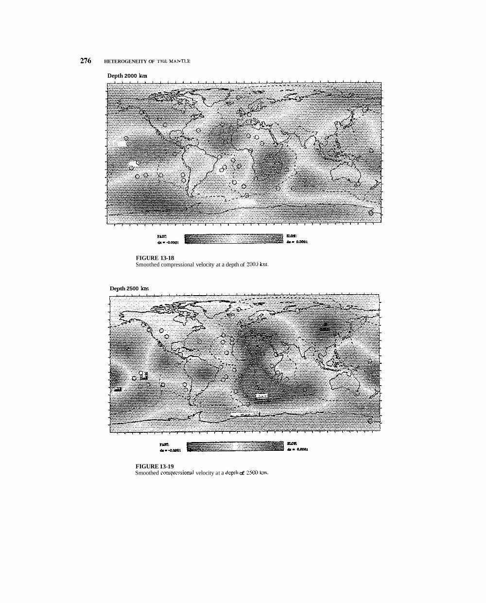
dent. In the top part of the lower mantle (Figure 13- 16), the prominent low-velocity regions are under the Indian Ocean, the western Pacific and China, south of New Zealand, the central Atlantic, the East Pacific Rise and the central Pa- cific. The fastest regions are Siberia, south Africa, south of South America and the northeast Pacific. At mid-to-lower mantle depths (Figures 13-17 and 13-18), the slowest re- gions are southeast Africa and adjacent Indian Ocean, the Cape Verde-Canaries-Azores region of the Atlantic, and the equatorial Pacific. The fast regions are in the north polar regions, North America, the southern Pacific, eastern In- dian Ocean and the South Atlantic. Most continental re- gions are fast. Near the base of the lower mantle (Figure 13- 19), the prominent low-velocity regions are southern and northern Africa, Brazil and the south-central Pacific. The fast regions are Asia, the North Atlantic, the northern Pa- cific and Antarctica. The locations of hotspots do not cor- relate with the slower regions at the base of the mantle.

The slow regions are presumably hotter than average and therefore probably represent buoyant upwellings, which in turn are responsible for geoid highs. They will tend to reorient the Earth so as to lie in low latitudes. This brings colder than average mantle into the polar regions. This, in turn, will affect convection in the core-cold downwellings in the core should occur preferentially in the polar regions and beneath the other fast regions at the base of the mantle. The colder regions of the lower mantle should have the highest temperature gradients at the base of the mantle, in

D". These are the regions where core heat is most readily removed. Heat flow from the core is probably far from uniform.

General References

Anderson, D. L. (1987) The depths of mantle reservoirs. In Mag- matic Processes (B . 0 . Mysen, ed.), Geochemical Society, Special Publication No. 1.

Grand, S. P. (1986) Shear velocity structure of the mantle beneath the North American plate, Ph.D. Thesis, California Institute of Technology.

Hager, B. H. (1983) Global isostatic geoid anomalies for plate and boundary layer models of the lithosphere, Earth Planet. Sci. Lett., 63, 97-109.

Hager, B. H: (1984) Subducted slabs and the geoid; constraints on mantle rheology and flow, J. Ceophys. Res., 89, 6003-6015.

Hager, B. H. and R. J. O'Connell (1979) Kinematic models of large-scale mantle flow, J. Ceophys. Res., 84, 1031-1048.

Haxby, W. and D. Turcotte (1978) On isostatic geoid anomalies, J. Geophys. Res., 83, 5473.

References

Anderson, D. L. (1967) Latest information from seismic obser- vations. In The Earth's Mantle (T. F. Gaskell, ed.), 355-420, Academic Press, New York.

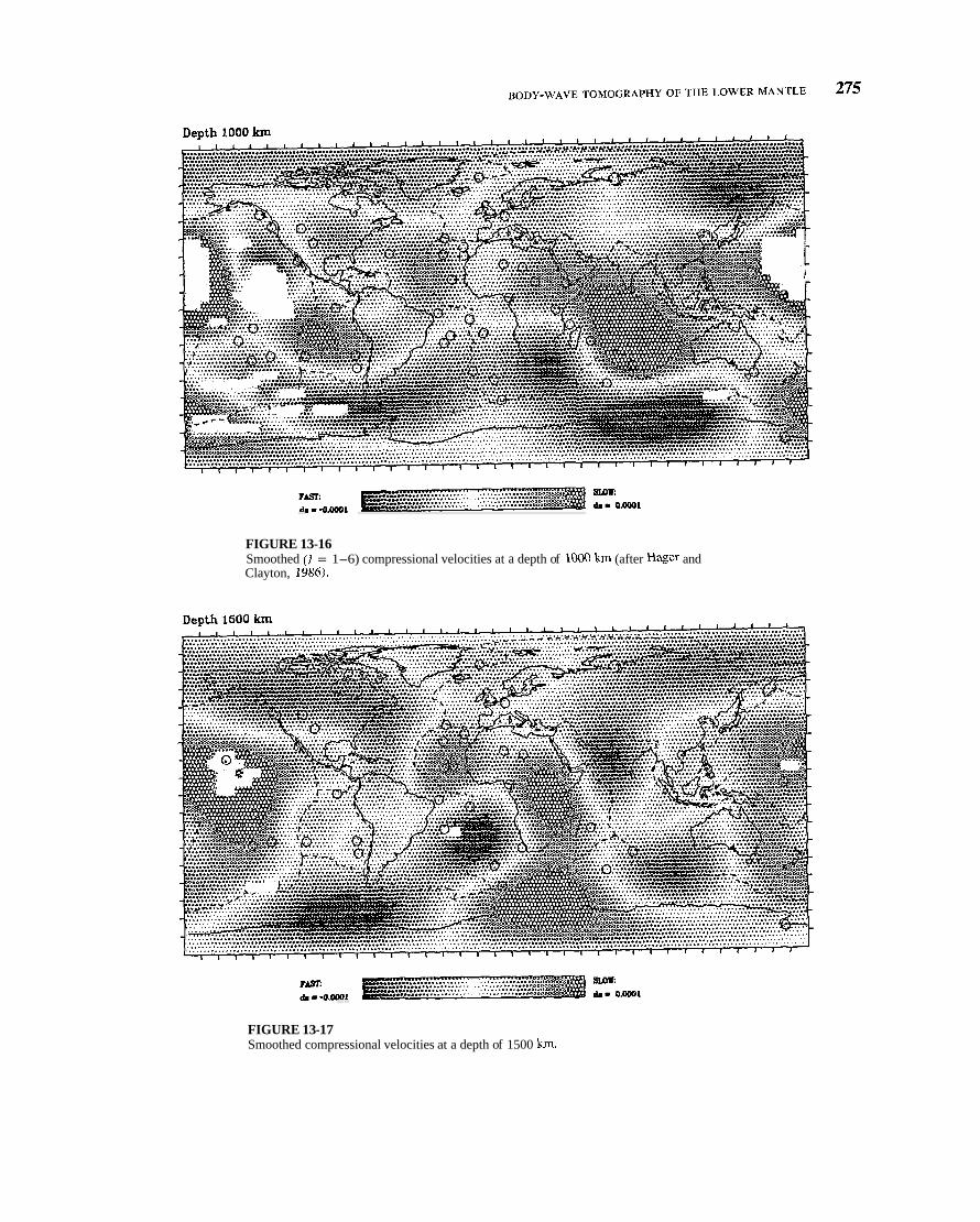
FIGURE 13-16 Smoothed (1 = 1-6) compressional velocities at a depth of 1000 km (after Hager and Clayton, 1986).

FIGURE 13-17 Smoothed compressional velocities at a depth of 1500 km.

HETEROGENEITY OF Tfl-E MAWTLE

Depth 2000 km

FIGURE 13-18 Smoothed compressional velocity at a depth of 2000 km.

Depth 2500 km

FIGURE 13-19 Smoothed compressional velocity at a depth of 2.500 km.

Anderson, D. L. (1979) The deep structure of continents, J. Geo- phys. Res., 84, 7555-7560.

Forsyth, D. W. (1975) The early structural evolution and anisot- ropy of the oceanic upper mantle, Geophys. J. R. Astron. Soc., 43, 103-162.

Grand, S. P. and D. V. Helmberger (1984a) Upper mantle shear structure of North America, Geophys. J. Roy. Astron. Soc., 76, 399-438.

Grand, S. P. and D. V. Helmberger (1984b) Upper mantle shear structure beneath the Northwest Atlantic Ocean, J. Geophys. Res., 89, 11,465-1 1,475.

Graves, R. and D. V. Helmberger (1987) J . Geophys. Res., 93, 4701-4711.

Hager, B. H. and R. Clayton, Constraints on the structure of mantle convection using seismic observations, flow models and the geoid (in press), 1987.

Jordan, T. H. (1975) The continental tectosphere, Rev. Geophys. Space Phys., 13, 1-12.

Morris, E. M., R. W. Raitt and G. G. Shor (1969), J. Geophys. Res., 74, 4300-4.316.

Nakanishi, I. and D. L. Anderson (1983) Measurements of mantle wave velocities and inversion for lateral heterogeneity and an- isotropy: Part I, Analysis of great circle phase velocities, J. Geophys. Res., 88, 10,267- 10,283.

Nakanishi, I. and D. L. Anderson (1984a) Aspherical heteroge- neity of the mantle from phase velocities of mantle waves, Na- ture, 307, 117-121.

Nakanishi, I . and D. L. Anderson (1984b) Measurements of mantle wave velocities and inversion for lateral heterogeneity and an- isotropy: Part 11, Analysis by single-station method, Geophys. J. Roy. Astron. Soc., 78, 573-617.

Nataf, H.-C., I. Nakanishi and D. L. Anderson (1984) Anisotropy and shear velocity heterogeneities in the upper mantle, Geo- phys. Res. Lett., 11, 109-112.

Nataf, H.-C., I. Nakanishi and D. L. Anderson (1986) Measure- ments of mantle wave velocities and inversion for lateral hetero- geneities and anisotropy: 111, Inversion, J. Geophys. Res., 91, 7261-7308.

Okal, E. A. and D. L. Anderson (1975) A study of lateral inhomo- geneities in the upper mantle by multiple ScS travel-time re- siduals, Geophys. Res. Lett., 2 , 313-316.

Sipkin, S. A. and T. H. Jordan (1976) Lateral heterogeneity of the upper mantle determined from the travel times of multiple ScS, J. Geophys. Res., 81, 6307-6320.

Tanimoto, T. and D. L. Anderson (1984) Mapping convection in the mantle, Geophys. Res. Lett., 11, 287-290.

Tanimoto, T. and D. L. Anderson (1985) Lateral heterogeneity and azimuthal anisotropy of the upper mantle: Love and Ray- leigh waves 100-250 sec., J. Geophys. Res., 90, 1842- 1858.

Toksoz, M. N. and D. L. Anderson (1966) Phase velocities of long-period surface waves and structure of the upper mantle, 1. Great circle Love and Rayleigh wave data, J. Geophys. Res., 71, 1649-1658.

Walck, M. C. (1984) The P-wave upper mantle structure beneath an active spreading center; the Gulf of California, Geophys. J. Roy. Astron. Soc., 76, 697-723.

Woodhouse, J. H. and A.M. Dziewonski (1984) Mapping the upper mantle: Three-dimensional modeling of earth structure by inversion of seismic waveforms, J. Geophys. Res., 89, 5953-5986.