Theory of Production

Production Function defined:

• The PF is a statement of the relationship between a firm’s scarce resources (inputs) and the output that results from the use of these resources.

• In mathematical terms, the PF can be expressed as:

• Q= f (X1, X2…………Xk) where • Q=output, X1…………Xk=inputs used in

the production process

Formal definition of PF

• A PF defines the relationship between inputs and the maximum amount that can be produced within a given period of time with a given level of technology.

• For the purposes of analysis, we write the PF as follows: Q= f (L, K)

• Where Q=output, L= labour, K=capital

A short-Run Analysis of Total, Average and Marginal Product

• Marginal product of Labor =MPL= ∆Q/∆L, holding K constant.

• Average product of Labor= APL= Q/L, holding K constant.

Short run changes in productionUnits of K employed

Output quantity

8

7

6

5

4

3

K=2 8 18 29 39 47 52 56 52

1

1 2 3 4 5 6 7 8(Units of L employed)

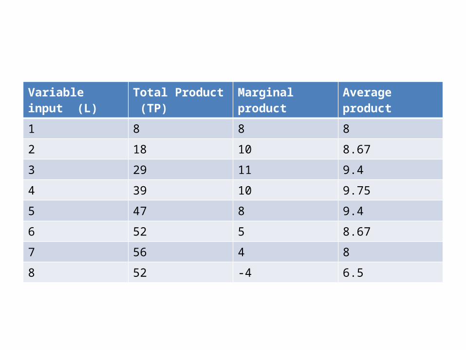
Variable input (L) Total Product (TP) Marginal product Average product

1 8 8 8

2 18 10 8.67

3 29 11 9.4

4 39 10 9.75

5 47 8 9.4

6 52 5 8.67

7 56 4 8

8 52 -4 6.5

The Three Stages of Production in the Short-run

• Stage I runs from zero to four units of variable input (where average product reaches its maximum and AP and MP are approximately equal).

• Stage II begins from this point and proceeds to seven units of input L (to the point where TP is maximised).

• Stage III continues on from that point.

Law of Diminishing Returns

• The key to understanding the pattern of change in Q, AP and MP is the phenomenon known as the Law of diminishing returns:

• As additional units of variable input are combined with a fixed input, at some point the additional output (the MP) starts to diminish.

Which stage is economical or rational?

• According to economic theory, in the short-run, rational firms should only be operating in stage II.

• It is clear why stage III is irrational: the firm would be using more of its variable input to produce less output.

• However, it may not be as apparent why stage I is also considered irrational.

• The reason is that if a firm were operating in stage I, it would be grossly underusing its fixed capacity.

• That is, it would have so much fixed capacity relative to its usage of variable inputs that it could increase the output per unit of variable input simply by adding more variable inputs to this capacity.

Derived Demand and the optimal level of variable input case (The case of one input case)

Optimal decision rule: A profit maximising firm operating in perfectly competitive output and input markets will be using the optimal amount of an input at the point at which the monetary value of input’s marginal product is equal to the additional cost of using that input---in other word’s when MRP=MLC.

Optimal Input Usage Rule (one input Case when price of product=$2 and labor cost=$10)Labor Unit (L)

Total Product

Marginal Product

Total Revenue Product

Marginal Revenue Product

Total labor cost

Marginal labor cost

1 10 10 20 20 10 10

2 25 15 50 30 20 10

3 45 20 90 40 30 10

4 60 15 120 30 40 10

5 70 10 140 20 50 10

6 75 5 150 10 60 10

7 78 3 156 6 70 10

8 80 2 160 4 80 10

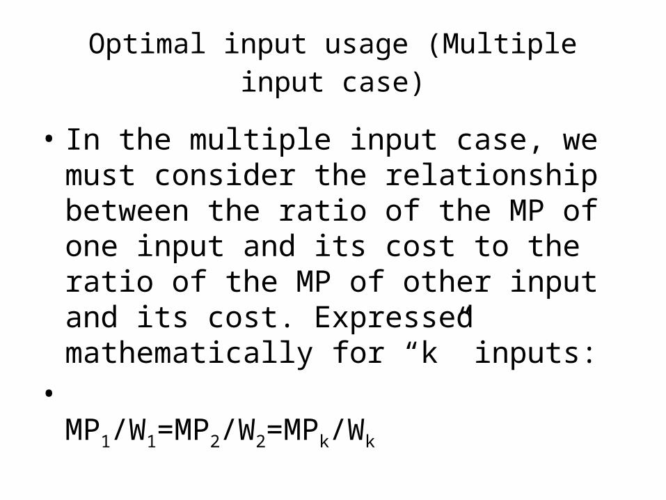
Optimal input usage (Multiple input case)

• In the multiple input case, we must consider the relationship between the ratio of the MP of one input and its cost to the ratio of the MP of other input and its cost. Expressed mathematically for “k” inputs:

• MP1/W1=MP2/W2=MPk/Wk

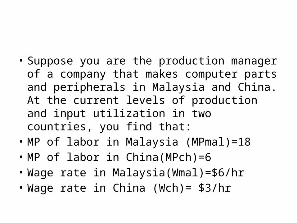
• Suppose you are the production manager of a company that makes computer parts and peripherals in Malaysia and China. At the current levels of production and input utilization in two countries, you find that:

• MP of labor in Malaysia (MPmal)=18• MP of labor in China(MPch)=6• Wage rate in Malaysia(Wmal)=$6/hr• Wage rate in China (Wch)= $3/hr

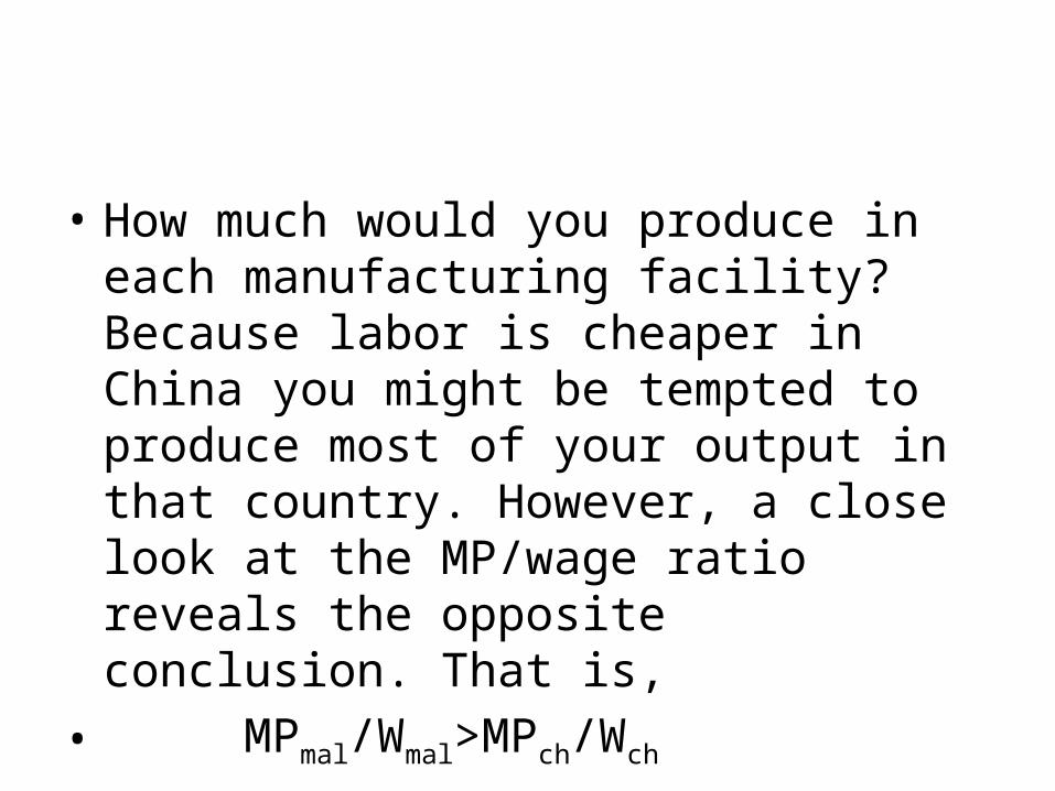
• How much would you produce in each manufacturing facility? Because labor is cheaper in China you might be tempted to produce most of your output in that country. However, a close look at the MP/wage ratio reveals the opposite conclusion. That is,

• MPmal/Wmal>MPch/Wch

• Or 18/6 > 6/3

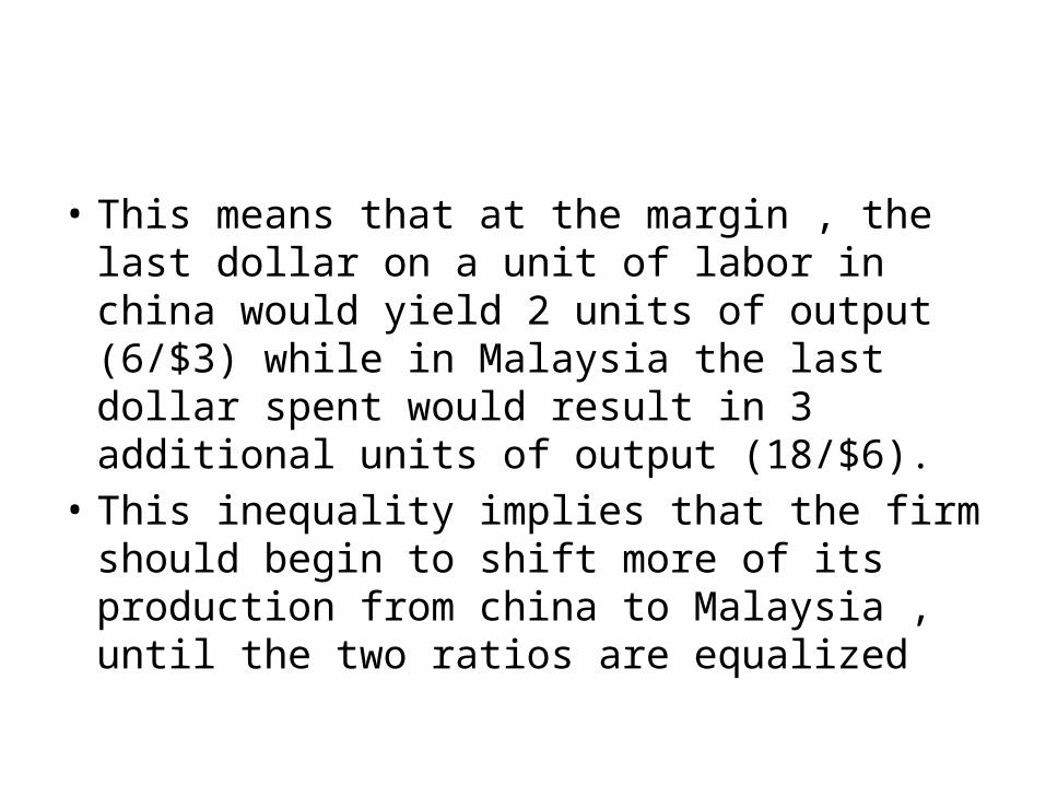
• This means that at the margin , the last dollar on a unit of labor in china would yield 2 units of output (6/$3) while in Malaysia the last dollar spent would result in 3 additional units of output (18/$6).

• This inequality implies that the firm should begin to shift more of its production from china to Malaysia , until the two ratios are equalized

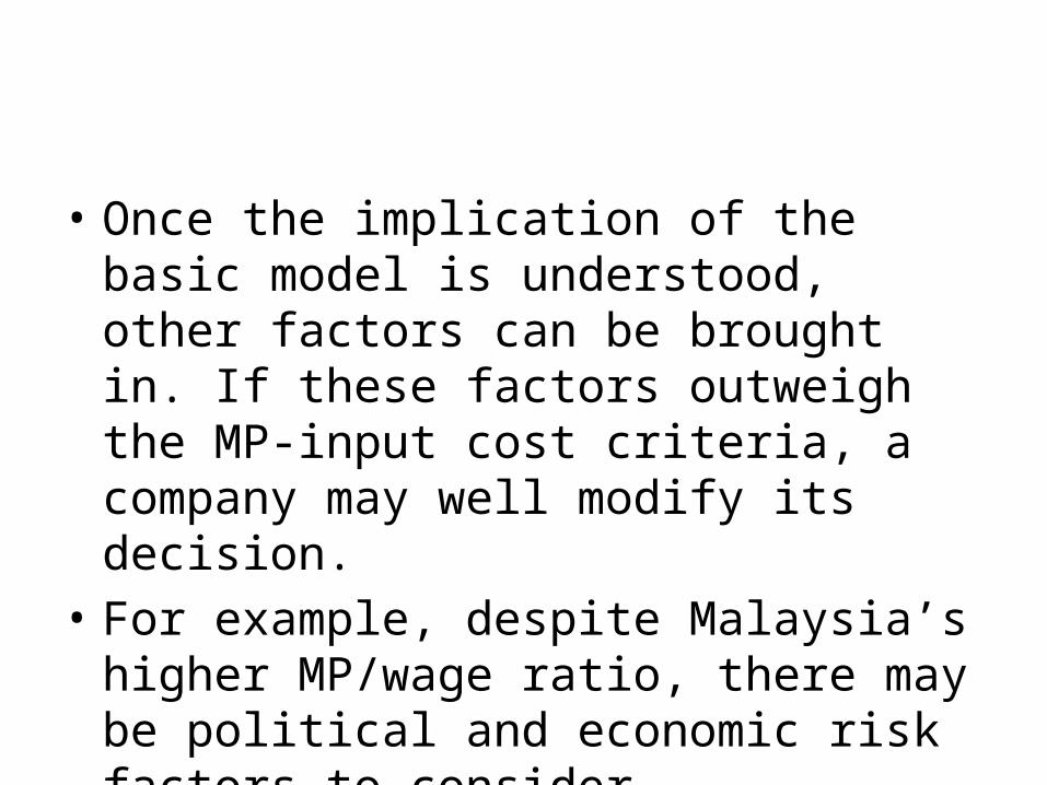
• Once the implication of the basic model is understood, other factors can be brought in. If these factors outweigh the MP-input cost criteria, a company may well modify its decision.

• For example, despite Malaysia’s higher MP/wage ratio, there may be political and economic risk factors to consider.

• This was indeed the case when the Malaysian government imposed foreign exchange controls in 1998 by requiring foreign investors to keep their profits in Malaysia for at least 1 year before they could be repartriated .

• In contrast, China is a fairly stable economy with leaders who do not seem to want to impose any such trade restrictions. Its proximity to Indian markets would also would also reduce transportation costs.

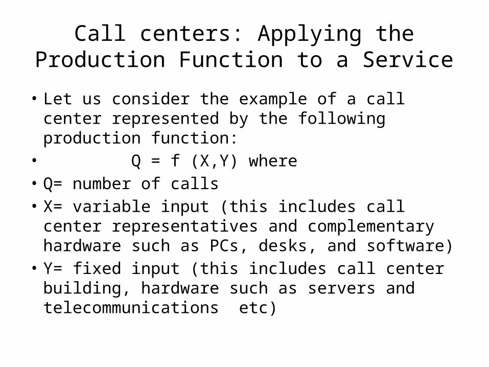
Call centers: Applying the Production Function to a Service

• Let us consider the example of a call center represented by the following production function:

• Q = f (X,Y) where• Q= number of calls • X= variable input (this includes call center

representatives and complementary hardware such as PCs, desks, and software)

• Y= fixed input (this includes call center building, hardware such as servers and telecommunications etc)

Three Stages of production

• Stage I could be a situation in which there is so much fixed capacity relative to number of variable inputsthat many representatives sit around idle, waiting for calls to come in.

• Stage II could be a situation in which representatives are constantly occupied and callers are connected to representatives immediately after the call is answered or are kept waiting for no more than a certain amount of time (3 min).

• Stage III could be a situation in which callers begin to experience a busy signal on a more frequent basis or all call representatives may begin to experience a slower computer response or more frequent computer ‘down times’.

The Long Run Production Function

• In the long run, a firm has time enough to change the amount of all inputs. The following Table illustrates what happens to total output as both inputs L and K increase one unit at a time.

Returns to ScaleUnits of K employed

Output

Quantity

8 125

7 119

6 90

5 75

4 60

3 41

2 18

1 4

1 2 3 4 5 6 7 8 Units of L employed

• The resulting increase in output as both inputs vary is known as Returns to Scale.

• Returns to scale are of three types:• Increasing returns to scale• Decreasing returns to scale• Constant returns to scale

• If an increase in a firm’s input by some proportion results in an increase in output by a greater proportion, the firm experiences IRTS.

• If output increases by the same proportion as the inputs increase, the firm experiences CRTS.

• A less than proportional increase in output is called decreasing returns to scale.

• One way to measure RTS is to use the coefficient of output elasticity:

• EQ= % change in Q/% change in inputs• If EQ>1, we have IRTS• If EQ<1, we have DRTS• If EQ=1, we have CRTS

• Another way of looking at the concept of RTS is based on the production function: Q = f (L, K)

• Now if we increase both inputs by r times and output increases by t times, that is

• tQ= f(rL, rK) then • If t>r, we have IRTS• If t<r, we have DRTS• If t=r, we have CRTS.

The Cobb-Douglas Production Function

• The C-D production function was introduced in 1928 and it is still a common functional form in economic studies today.

• It has been used extensively to estimate both individual firm and aggregate production function.

• The formula for production function which was suggested by Cobb, was of the following form: Q= aLbK1-b

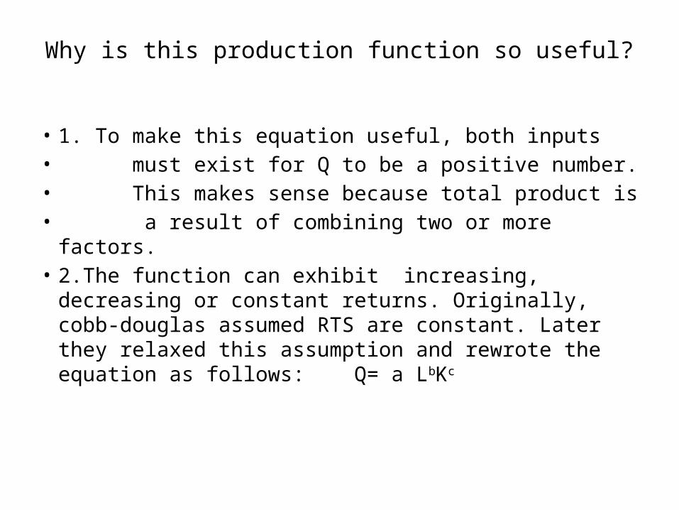
Why is this production function so useful?

• 1. To make this equation useful, both inputs• must exist for Q to be a positive number.• This makes sense because total product is• a result of combining two or more factors.• 2.The function can exhibit increasing,

decreasing or constant returns. Originally, cobb-douglas assumed RTS are constant. Later they relaxed this assumption and rewrote the equation as follows: Q= a LbKc

• Under this assumption if b+c>1, RTS are increasing, if b+c<1, RTS are decreasing and if b+c=1, RTS are constant.

• 3. The function permits us to investigate the MP for any factor while holding all others constant. MP of labor turns out to be MPL=bQ/L and MP of capital is MPk=cQ/K.

• In the C-D function, the elasticities of the factors are equal to their exponents, in this case b and c.

• 4.Because a power function by using logarithms, it can be estimated by linear regression analysis, which makes for a relatively easy calculation with any software package.

• 5. Cobb-Douglas can accommodate any number of independent variables as follows:

• Q=aXb1Xc

2Xd3..Xm

n

• 7. A theoretical production function assumes technology is constant. However, the data fitted by the researcher may span a period over which technology has progressed. One of the independent variables in the previous equation could represent technological change and thus adjust the function to take any technology into consideration.

Shortcomings of C-D production Function

• This function cannot show the MP going through all three stages of production in one specification.

• Similarly, it cannot show a firm or ndustry passing through increasing, constant and decreasing returns to scale.