theory of interlayer exchange coupling - max planck …bruno/publis/1995_6.pdfphysical revlew b...

PHYSICAL REVLEW B VOLUME 52, NUMBER 1 1 JULY f995-I

Theory of interlayer magnetic coupling

P. Bruno* Imtdtut d’Electmnique Fondamentale, Bcitiment 220, Universittt Paris-Sud, F-91405 Orsaql, France

(Received 28 November 1994)

A theory of interlayer exchange coupling is presented. A detailed and comprehensive discussion of the various aspects of the problem is given. The interlayer exchange coupling is described in terms of quantum interferences due to confinement in ultrathin layers. This approach provides both a physically transparent picture of the coupling mechanism, and a suitable scheme for discussing the case of a realistic system. This is illustrated for the Co/Cu/Co(OOI) system. The cases of metallic and insulating spacers are treated in a unified manner by introducing the concept of the complex Fermi surface.

I. INTRODUCTION

Since the first observation by Griinberg et al.’ of antiferromagnetic coupling of Fe films separated by a Cr spacer, the interlayer exchange interaction between ferromagnetic layers separated by a nonmagnetic spacer has been a subject of intense research in the last few years. The decisive stimulus came &om the discovery, by Parkin et of oscillations of the interlayer exchange coupling in Fe/Cr/Fe and Co/Ru/Co multilayers, as a function of spacer thickness. Furthermore, Parkin3 showed that this spectacular phenomenon occurs with almost any transition metal as a spacer material.

Investigations of interlayer exchange coupling across nonmetallic spacer layers have been pioneered by Toscano et al.,* who studied the coupling of Fe films separated by amorphous Si. A striking feature is that the cou- pIing, in contrast to the case of a metal spacer, increases with increasing temperature.’ Furthermore, Mattson et aL6 found that the coupling across a FeSi spacer may be induced by illumination by visible light; this behavior, however, remains controver~ial.~

For the case of metal spacers, a great number of theoretical studies has been performed, essentially focusing on the oscillatory character of the coupling. There are essentially two classes of approaches to this problem: total- energy calculations and model calculations.

The idea of the former approach is to compute the total energy of the system for configurations of parallel and antiparallel alignment of the magnetizations in neighboring magnetic layers, and to identify the energy difference with the interlayer exchange coupling. Such calculations have been performed either within semiempirical tight- binding models8 or ab initio scherne~.~- l~ Although it is very simple and straightforward in principle, this kind of approach is actually very difficult. The point is that the energy difference between the parallel and antiparallel configurations is tiny (of the order of 1 meV or less, per unit cell), whereas the total energy is large. This makes numerical convergence of the calculations a serious problem. Furthermore, as the computation time increases very rapidly with the size of the unit cell, total-

52 -

energy calculations are usually restricted to small layer thicknesses, which makes the investigation of long-period oscillations problematic. Another difficulty concerns the interpretation of the results: One usually has to perform a Fourier analysis of the coupling versus spacer thickness to identify the oscillation periods, whose interpretation then relies on various models. In spite of these difficulties, total-energy calculations have encountered encour- aging success, a t least as far as oscillation periods are concerned. Nevertheless, the coupling strengths obtained from total-energy calculations are typically one order of magnitude larger (or even more) than the experimental ones (for a review see Ref. 14). Thus, complete eluci- dation of interlayer coupling from this kind of approach remains a serious challenge. In order to circumvent the difficulties mentioned above,

various models have been devised to get some better insight in the mechanism of interlayer exchange coupling. These are (i) the Ruderman-Kittel-Kasuya-Yosida (RKKY) in which the magnetic layers are described as arrays of localized spins interacting with conduction electrons by a contact exchange potential, (ii) the free-electron of which many variants have been proposed, (iii) the hole confinement which is essentially a tight-binding model with spin-dependent potential steps, and (iv) the Anderson (or sd-mixing) m ~ d e l . ~ * ! ~ ~

The great advantage of these models is that their simplicity allows one to obtain analytical results, thus making the physics transparent. In particular, all the models relate the oscillation periods, in the limit of large spacer thicknesses, to the Fermi surface of the bulk spacer material.

The general criterion giving the oscillation periods for an arbitrary (nonspherical) Fermi surface has been given by Bruno and Chappert in the context of RKKY theory.17 They have used this criterion to predict the oscillation periods for noble metal spacers, whose Fermi surface is fairly simple and known accurately from de Haas-van Alphen experiments.26 These predictions have been confirmed successfully by numerous experimental observations; in particular, the coexistence of a long and

41 1 @ 1995 The American Physical Society

52 412 P. BRUNO -

a short period for the (001) orientation has been found for both noble metal^,^^-^^ in good quantitative agreement with RKKY theory. Further evidence of the validity of the relationship between the oscillation periods and the Fermi surface of the spacer has been obtained by varying systematically the number of valence electrons via a l l~ying .~"-~~ The criterion given by Bruno and Chap- pert has been used by Stiles33 to determine the oscillation periods for transition metal spacers; however, the Fermi surfaces are so complicated, and the periods so numerous, that a reliable comparison with experimental results seems very doubtful.

Concerning the strength of the coupling, a general trend obtained from the above models is that it depends essentially on the degree of matching of the energy bands at the paramagnet-ferromagnet interface; this appears very clearly from the free-electron model, the hole confinement model, and the sd-mixing model. This trend seems to be supported by the experimental results of Parkin3 for transition metal spacers; however, because of the drastic idealization of these models, no quantitative predictions for realistic systems have been given so far.

In a recent paper, I proposed a general approach to the problem of interlayer coupling,34 which offers a suitable starting point for realistic calculations, and at the same time provides deep physical insight into the mechanism of interlayer coupling. In this approach, the interlayer exchange coupling is described in terms of the quantum interferences due to the (spin-dependent) reflections of Bloch waves at the paramagnet-ferromagnet interfaces. In its most general formulation, this approach embod- ies all the models mentioned above as particular cases, thus identifying clearly the features that are generic to the phenomenon of interlayer coupling, and the ones that depend on specific assumptions of a given model. Essen- tially the same formulation has been subsequently presented by Stiles,33 who derived the expression of the coupling directly in terms of the wave functions, instead of using Green's functions as in Ref. 34.

Until recently, it was generally believed that the interlayer coupling is independent of the magnetic layers thickness.35 On the other hand, Barn&" found from numerical calculations for the free-electron model that the coupling oscillates versus magnetic layer thickness; however, the origin of this behavior remained unclear. As I discussed in Ref. 36, it becomes almost obvious, in the light of the "quantum interference" formulation, that one may expect such oscillations, as a consequence of the interferences associated with the multiple internal reflections in a magnetic layer of finite thickness, in analogy with the reflection oscillations in an optical Fabry-PBrot cavity. This prediction has been confirmed recently by Bloemen et in Co/Cu/Co(OOl) and by Okuno and Inomata in Fe/Cr/Fe(001).38

In contrast to the important theoretical literature devoted to interlayer coupling across a metal spacer, the magnetic coupling across insulators has attracted very little attention from the theoretical point of view. A no- table exception is Slonczewski's model of coupling, at T = 0, through a tunneling barrier:39 The coupling in

this case is nonoscillatory, and decays exponentially with spacer thickness. In a recent paper,40 I discussed this problem within the quantum interference approach: At T = 0, one obtains essentially the same results as Slon- czewski; on the other hand, the coupling is found to increase with increasing temperature, in contrast to the metal spacer case.

One great virtue of the quantum interference approach is that it allows one to treat metal and illsulator spacers in a unified manner, by using the concept of a complex Fermi surface, as discussed in Ref. 40.

The purpose of the present paper is to give a comprehensive and extended discussion of the theory presented in Refs. 34, 36, and 40. It is organized as follows: In view of pedagogical clarity, after a heuristic presentation of the physical mechanism of interlayer coupling and of the underlying concepts (Sec. 11), I shall illustrate the theory within the simple free-electron model (Sec. 111). In Sec. IV, I shall present the material necessary to the general theory of interlayer coupling; in particular, the concept of complex Fewni surface will be introduced. The general theory of interlayer coupling will be presented in Sec. V. In Sec. VI, I discuss the connection between the present approach and the various models that have been used to study the problem of interlayer coupling. Then, I will present, in Sec. VII, the complex Fermi surfaces of noble metals, as calculated by using the linear rnuffin-tin orbital (LMTO) method. In Sec. VIII, I shall discuss how to calculate the reflection and transmission coefficients for realistic multiband systems. Finally, Sec. IX is devoted to the discussion of a realistic case: namely, CU/CO (001).

11. QUANTUM INTERFERENCES AND INTERLAYER EXCHANGE COUPLING

In this section, I shall present a heuristic presentation of the interlayer coupling in terms of quantum interferences in the spacer layer; the emphasis will be on physical transparency rather than on mathematical strictness.

A. One-dimensional model

To start with, I shall &st consider a simple one- dimensional model. The model consists of a spacer layer of width D and potential V = 0, sandwiched between two potential perturbations A and B of respective widths LA and LB, and respective heights VA and VB. Outside the perturbations, the potential is equal to zero, and the widths LA and LB may be finite or infinite. Positive values for VA and VB correspond to potential barriers, whereas negative values correspond to potential wells.

1. Change of density of states due to the quantum intepferences

Let us consider an electron of wave vector I c l (with kl > 0) traveling in the spacer towards the right; as this

- 52 THEORY OF INTERLAYER MAGNETIC COUPLING 413

electron encounters the perturbation B, it is reflected with a (complex) amplitude rg = Irg/ei+B. The reflected wave, of wave vector - k l , is in turn reflected on A with amplitude T A G IrAlei+A, and so on. The module I T A ( B ~ I of the reflection coefficient gives the magnitude of the reflected wave, while the argument q 5 ~ ( ~ ) gives the phase shift due to the reflection (note that the latter is not absolute and depends on the choice for the coordinate origin).

The multiple interferences that take place in the spacer induce a change in the density of space. The phase shift of the wave function after a complete round trip in the spacer is

A + = ~ ~ L D + + A + + B . (2 .1)

Clearly, if the interferences are constructive, i.e., if

Aq5 = 2n1r , (2.2a)

with n an integer, one has an increase of the density of states; conversely, when the interferences are destructive, i.e.,

Aq5 = (2n + l ) n , (2.2b)

the density of states decreases. Thus, in a first approximation, the change of density of states due to interferences, An(&), should vary like c o s ( 2 k l D + 4 A + + E ) ; furthermore, it should be proportional to the strength of the reflections on A and B, i.e., to I T A T E ] ; finally it is proportional to the spacer width D and to the density of states per unit length and energy :%. There is also a factor of 2 for spin degeneracy. Thus we find

It is more convenient to consider the integrated density of states (the number of states of energy lower than E ) :

N ( E ) l L n ( & ’ ) d&‘ . (2 .4)

The change A N ( E ) of the integrated density of states is

where the energy derivative of the reflection coefficients has been neglected compared to the energy derivative of the exponential factor, which is a good approximation if D is large.

The above derivation of the change of integrated density of states is not rigorous, but allows a clear physical understanding of the effect of the quantum interferences in the spacer. It is valid when the reflection coefficients are small, so that higher-order terms may be neglected. On the other hand, if I T A ~ = I T B ~ = 1, the interferences lead to bound states and the wave vector k l is quan- tized; the bound states occur when the interferences are

constructive, i.e., when

with n an integer. As D increases, the bound states move towards lower energy and the integrated density of states jumps each time a bound state has energy E.

The product ~ T A T B ~ measures the strength of the electron confinement in the spacer. As will be shown in Sec. V, the exact expression of the change in the integrated density of states due to quantum interferences is

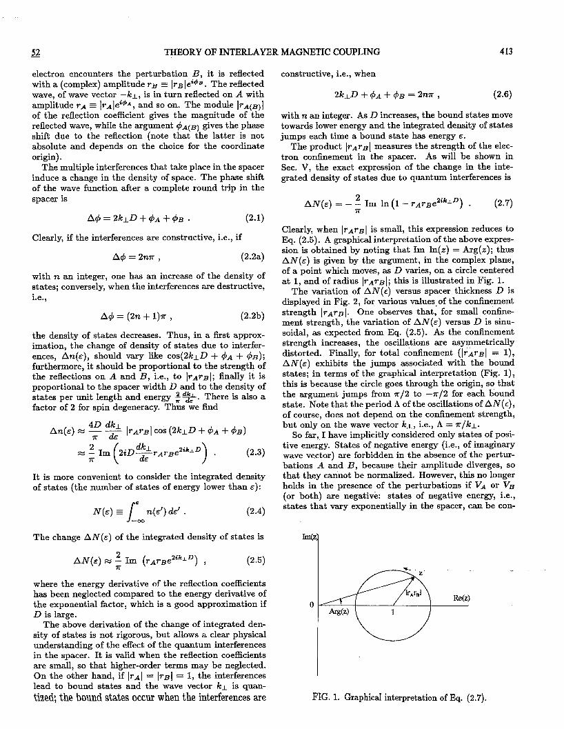
2 AN(&) = - - Im In (1 - rArgeZikLD) . (2 .7) ?r

Clearly, when ~ T A T B I is small, this expression reduces to Eq. ( 2 . 5 ) . A graphical interpretation of the above expression is obtained by noting that Im ln(z) = Arg(z); thus A N ( & ) is given by the argument, in the complex plane, of a point which moves, as D varies, on a circle centered at 1, and of radius ~ ~ A T B I ; this is illustrated in Fig. 1.

The variation of A N ( € ) versus spacer thickness D is displayed in Fig. 2 , for various values,of the confinement strength ~ ~ A T B I . One observes that, for small confinement strength, the variation of AN(&) versus D is sinu- soidal, as expected from Eq. ( 2 . 5 ) . As the confinement strength increases, the oscillations are asymmetrically distorted. Finally, for total confinement (lTA1“Bl = I), AN(&) exhibits the jumps associated with the bound states; in terms of the graphical interpretation (Fig. l), this is because the circle goes through the origin, so that the argument jumps from 7r/2 to -7r/2 €or each bound state. Note that the period A of the oscillations of AN(€), of course, does not depend on the confinement strength, but only on the wave vector k i , i.e., A = n / k l .

So far, I have implicitly considered only states of positive energy. States of negative energy (i.e., of imaginary wave vector) are forbidden in the absence of the perturbations A and B, because their amplitude diverges, so that they cannot be normalized. However, this no longer holds in the presence of the perturbations if VA or VB (or both) are negative: states of negative energy, i.e., states that vary exponentially in the spacer, can be con-

I

FIG. 1. Graphical interpretation of Eq. (2.7).

4 s4 52 P. BRUNO -

0.0

0.0

1 (c) lrArBl= 1

I 1 1 1 1 ~ 1 1 l I ~ I l l I I I I I I ( I l l l

0.0 1 .o 2.0 3.0 4.0 5.0 kiD/ n

FIG. 2. Variation of the change of integrated density of states due to quantum interferences, AN(&), vs spacer thickness D, as given by Eq. (2.7), for various values of the confinement strength: (a) IrArBl = 0.1, (b) IrArBI = 0.8, (c) IrArBI = 1 (total confinement).

nected to allowed states in A or B. To treat these states consistently, we extend the concept of reflection coefficients to the states of imaginary wave vectors. One can check that, with this generalization, Eq. (2.7) accounts completely for the effect of the states of negative energy (evanescent states). A detailed discussion of their role will be presented in the following sections of the paper.

2. Energy associated with the quantum interferences

Let us now estimate the energy change, at T = 0, of the system, due to the quantum interferences in the spacer. To ensure conservation of the number of particles, it is convenient to work in the grand-canonical ensemble, and to use the grand potential, which is, at T = 0,

E F

@ 3 1, (E - E F ) +),& ; (2.8)

integrating by parts, this yields,

(2.9)

Thus the energy change due to the quantum interferences is

For small confinement, this becomes

.,~ . , >- ." - BF

..ii._ . ".&&U" . '"''""""2 li- II

AE M - - Im J__ TATBeZik-LD dE . (2 .11)

One'seeS that states for which the interferences are constructive (destructive) contribute to a repulsive (attrac- tive) force between A and B. Hereafter, AE will be called the coupling energy.

B. Three-dimensional layered system

The generalization of the above discussion to the more realistic case of a three-dimensional layered system is im- mediate. It follows from the fact that, since the potential depends only on the coordinate in the direction normal to the layers, the in-plane component kll of the wave vector is a good quantum number. Thus, for each kll, we have an effective one-dimensional problem such as the one discussed above; the effect of the quantum interferences in the spacer is obtained by summing over kll. The change in the integrated density of states per unit area is

AN(&) = - - Im / d2kll In ( 1 - T A T B ~ ' ~ ' ~ ~ ) , 2n3

(2.12)

and the coupling energy per unit area is

(2 .13)

Of course, the reflection coefficients and the normal component of the wave vector k l are now functions, not only of the energy, but also of kll. For small confinement, the above expressions reduce, respectively, to

AX(&) M - Im d2kll rArBe2ikLD 2n3 ' J (2.14)

and

A E = - - h 1 d2k TATBP"~ d& . (2 .15) 2 s 3 J

C. Quantum interferences in overlayers

A situation of great physical interest is the one of an overlayer on a substrate. The overlayer is bounded on one side by the vacuum, which can be modeled by a semi-infinite potential barrier of height V,,, = EF + W , where W is the work function. The vacuum barrier is per- fectly reflecting for electrons below the vacuum level, i.e., lrvrrcl = 1. On the other side, the overlayer is bounded by the (semi-infinite) substrate material, with a reflection coefficent T .

The density of states in the overlayer below and above the Fermi level can be probed experimentally by using, respectively, direct and inverse photoemission spectroscopy. If, furthermore, one uses angle- resolved photoemission, one can probe the density of


states locally in the kit plane. As the thickness of the overlayer is varied, the photoemission signal exhibits oscillations, with a period given by the wave vector LI in the overlayer, and an amplitude proportional to Ir[.

In the case where the substrate is a ferromagnetic material, the reflection coefficient at the paramagnet- ferromagnet interface depends on the direction of the electron spin with respect to the magnetization direction in the ferromagnet; thus one has r t # r 4 . One then defines

- r t +r& 7-z- (2.16a)

2

and

r t - rJ A T E - ~ (2.16b)

respectively, the spin average and spin asymmetry of the reflection coefficients. If the photoemission experiment is performed in a spin-polarized mode, one observes oscillations in the intensity and spin polarization of the signal.

Observations of the quantum interferences due to confinement in overlayers have been reported by Ortega and Himpse141 from non-spin-polarized inverse photoemission on Cu overlayers on Co(OO1) and Ag overlayers on Fe(OO1). They suggested that these interferences should be attributed to minority-spin electrons, and are responsible for the oscillations of interlayer exchange coupling versus spacer thickness. Confirmation of their sug- gestion has been given by Garrison et ~ 1 . ~ ~ and Carbone et al.4s who performed spin-polarized photoemission experiments on Cu overlayers on Co(OOl), and showed that

I

2 '

the quantum interferences are actually spin dependent and mostly of minority-spin character.

D. Interlayer exchange coupling

In the case where two ferromagnetic films are separated by a paramagnetic spacer layer, the quantum interferences in the spacer induce an interlayer exchange interaction between the ferromagnetic layers.

In the ferromagnetic configuration, the energy due to the interferences, at T = 0, is

r

In the antiferromagnetic configuration, one has

r

1

so that the exchange coupling energy per unit area at T = O i s

(2.19)

which, for small confinement, reduces to

ArAArB eZikl dE . 1 EF - Enp M - - Im d2k x3 I Ill:

(2.20)

The above equation expresses transparently that the variation of the coupling versus spacer thickness depends only on the spacer material (via the wave vectors kl), whereas the strength and phase of the coupling are determined by the spin asymmetry of the reflection coefficients at the paramagnet-ferromagnet interfaces, which, in turn, depend on the degree of matching of the band structure on both sides of the interface. The implications of the above expression for the exchange coupling behavior will be presented in detail in the following section.

The quantum interference picture allows us to establish a quantitative connection between the quantum interferences in overlayers, as observed in photoemission experiments, and the interlayer exchange interaction. Whereas the latter results from the contribution of all allowed

I electron states, i.e., involves a summation over in-plane wave vector and energy, photoemission experiments offer the unique opportunity of being wave vector, energy, and spin selective; thus, it provides a powerful tool for investigating the mechanism of interlayer exchange coupling.44

111. FREE-ELECTRON MODEL

In this section, I discuss the problem of interlayer exchange coupling for the simple free-electron model. For this simple case, the calculations can be performed analytically, providing a physically transparent illustration of the various aspects of the problem.

The model-is as follows: The zero of energy is taken at the bottom of the majority band of the ferromagnetic layers; the potential of the minority band is given by the exchange splitting A, while the spacer, of thickness D , has a potential equal to U. The ferromagnetic layers have a thickness L, and their magnetizations are at an angle 8 with respect to each other. According to the position of the Fermi level, this model describes the case of a

52 416 P. BRUNO -

metallic spacer (for EF > U) or of an insulating spacer (for EF < U).

As will be demonstrated in Sec. V, the exact expression

correspond to evanescent states; both kinds of states contribute on an equal footing to the coupling in Eq. (3.1). Also, one has ck ,k+ = Ekll ,kL = E with kI = -k: and

for evanescent states.

I1 I Of the interlayer cOUPling energy Per unit area for an kf > 0, in the case of propagative states, 01 h(k: , f ) > 0, arbitrary angle 8 is

+w+io+ The expression of EAB (0) may be expanded in powers E u ( 0 ) = 2 h/cZ2kli / d & f ( e ) of cos e as

4x3 -w+io+ (el = J~ + J~ cos e + J~ cos2 8 + . - . , (3.2) X h [ I - 2 (FAFB 4- ArAArg COS 6 ) eiqLD

+ ( p i - AT:) (Fg - Ars ) eziqLD] , (3.1) where

where iO+ is an infinitesimal imaginary quantity, q 1 kt - kl, and f(&) is the Fermi-Dirac function. One can check easily that, taking the energy difference between the ferromagnetic (0 = 0) and antiferromagnetic (0 = K )

configurations in Eq. (3.1), one recovers the expression of the coupling [Eq. (2.19)] which has been obtained from a heuristic argument in the preceding section. The derivation of Eq. (3.1) involves integrations over RI &om -CO

to +CO, which are closed in the upper and lower complex half-planes, for the incident and reflected waves, respectively, by using the theorem of residues. There are two kinds of poles: Those lying on the real axis correspond to propagative states, while those lying off the real axis

r r+CO+iOf

x In 1 - 2F.4Fj3eiPLD

] (3.3)

[ + (PI - AT:) ( F ; - AT:) e2iqLD

I

is the nonmagnetic coupling constant, J1 is the Heisen- berg coupling constant, and J2 the biquadratic coupling constant; the general term of the expansion (3.2), for n 2 1, is given by

With the sign convention used here, a positive (negative) sign for Jl corresponds to an antiferromagnetic (ferromagnetic) interlayer exchange coupling.

Alternatively, one may take, as a measure of interlayer coupling, the energy difference per unit area between ferromagnetic (0 = 0) and antiferromagnetic (0 = T) configurations:

+m+i0+ EF - EAF = - 1 ImJd2kll/ & f ( ~ ) In [

--m+i0+ { 4x3

+w+io+ = - 1 Im/d2kll / & f ( ~ )

2T3 --m+i0+

I

The calculation of the reflection coefficients, for the 2 hzk;

tizk;

h2k l = & + io+ - - (3.8b) 2 m 2 m '

A, - - & + io+ - - -

free-electron model, is found in standard textbooks of quantum mechanic^.^^ Obviously, since the ferromag-

(3.8~)

respectively, and the sign of the imaginary part of k?') is the same as for kl. Obviously, the reflection coefficients for a state of wave vector k = (kll, k _ ~ ) are independent of kll , and depend only on ]GI.

In Eq. (3 .1) , the lower bound of the energy integration is -CO; on the other hand, states that are forbidden, Le., such that E < min(O,U), should not contribute to the coupling. One can check that this is actually the case, because for such states, both the reflection coefficients and the exponential factor are real, so that they give

netic layers are taken to be identical, ri2ki2 - 2 m 2 m

(3-6) rt(J.) = E r?(J- )* A ' B

Let ~8 consider &st the c s e of semi-infinite magnetic layers ( L = +CO); one finds

t(4) (3*7) Tt(J-) = f(J.) = kJ- - ICL

kl + Icy '

iiy

- 'pw

where

(3.8a) fi2k: - ----E+io+---u, 2 m 2 m


a vanishing contribution to the imaginary part, in the right-hand side of Eq. (3.1).

A. Metallic versus insulating spacer

1. Coupling at T = 0

At T = 0, one has

cp+io+

-w+io+ -w+io+ dE . (3.9) J +w+iO+

Changing the variable E for klf, and integrating over kll first, one obtains, for J1,

FIG. 3. Integration paths C and C' in the complex k i plane, in Eqs. (3.10) and (3.11): (a) metallic spacer (BF > U), (b) insulating spacer ( E F < U).

(3.10)

where the complex integration path C is shown in Fig. 3. The integrand in the above equation has no pole in the upper right quadrant of the complex plane and decreases exponentially as Im(kl) +CO; thus, one can replace, for the case of a metallic spacer, the integration path C by C', as shown in Fig. 3. This yields the result

valid for both cases, where the reflection coefficients are calculated for k: = kF + irc, with

k F = 1 / 2 m ( & ~ - U ) for E; > 0, (3.12a)

(3.12b)

respectively. For the energy difference between ferromagnetic and antiferromagnetic configurations, one gets .,.

EF - EAF = - dK K ( k F + k) ( 2 k ~ 4- k)

1 - 2A. r~ Arge2ikFDe-2KD xarctanh [ 1 - 2~Le-2uD~2ikp.D + (f& - e -4~De4 ikpD

(3.13)

Equations (3.11) and (3.13) allow very efficient numerical calculations of the coupling, because the integrand is not oscillatory, but exponentially decaying. It clearly shows that the thickness dependence of the coupling is driven by the factor e 2 i k F D ; thus the coupling oscillates with spacer thickness in the case of a metallic spacer (kF real), and decays exponentially with D for an insulating spacer ( k ~ imaginary). In the limit of large spacer thickness, and retaining only the leading contribution, Eq. (3.11) reduces to

h2 k$ 4 7 r 2 m D 2

J1 = Im (Ar,2e2ikFD) , (3.14)

where the reflection coefficients are calculated for k: = k ~ . In the case of an insulating spacer, the sign of the coupling at large spacer thicknesses is determined by the argument of A&; the coupling is antiferromag-

I

netic (ferromagnetic) if l k ~ l ' < k&kb (jkF12 > k&k$), where k s (kb) is the Fermi wave vector for majority-spin (minority-spin) electrons in the ferromagnet. At lower spacer thicknesses, the coupling may change sign, due to contributions originating from states well below E F .

Figures 4 and 5 show the coupling constant J1 calculated from Eq. (3.11), respectively, for a metallic spacer and for an insulating spacer.

Equation (3.14) is equivalent to the results obtained by Sloncew~ki~~ and by Erickson et U Z . , ~ O respectively, for the insulating spacer case and for the metal spacer case, by using Sloncewski's torque method.39

8. Thermal variation of the coupling

At finite temperature, after integration over kll, Eq. (3.4) for J1 becomes

418

100.0 I

0.0 5.0

metallic spacer

T=O

FIG. 4. Interlayer exchange coupling, at T = 0, for the Eree-electron model, in the case of a metallic spacer, calculated from Eq. (3.11). Parameters: L = +CO, E F = 7.0 eV, A = 1.5 eV, U = 0.

P. BRUNO

100.0 I

where

P k f 2 E l = - + U. 2m (3.16)

One can check easily that the above equation reduces to Eq. (3.11) for T = 0. For numerical calculations, it is more ef$ient to write

= J l ( 0 ) + AJl(T) , where Jl(0) is given by Eq. (3.11), and where

(3.17)

For large spacer thicknesses, the most important contribution to the coupling arises from the neighborhood of E F ;

the rapidly varying exponential factor ei2k:D, in the numerator of Eq. (3.151, may be expanded near EF as

this yields

(3.20)

I ature in the case of an insulating spacer ( k p imaginary). The integral may then be evaluated by performing the

The integral converges only if

(3.21) change of variable 1

Im(2mD/fi2kF) ' this is satisfied at any temperature in the case of a metallic spacer (kp real), but only at suf3ticiently low temper-

LBT =

(3.22)

- 52 THEORY OF INTERLAYER MAGNETIC COUPLING

I I I I

and by using the tabulated integral46

for - 1 < Re(p) < 0; (3.23)

the result is

where J1(0) is given by Eq. (3.14). In spite of the unified treatment given here, the temperature dependence of the coupling is strikingly different for a metallic and for an insulating spacer: In the former case, the coupling decreases with temperature, whereas in the latter, it increases. Formally, this is related to the fact that k~ is imaginary for an insulating spacer, and that

i X X

sinhix s i n ~ -=- (3.25)

is an increasing function, as shown in Fig. 6. Physically, the different behavior may be understood

from the simple following argument: In the case of a metallic spacer, the coupling, at T = 0, oscillates with a wave vector 2kF; as the temperature is raised, ICF is broadened with a width AkF M kBTm/fi2kF, which pro- duces a blurring of the coupling oscillations for D > Akil . In the case of an insulating coupling, on the other hand, the contribution to the coupling arising from electrons of energy E increases exponentially with E; as the temperature increases from zero, the contribution due electrons in an energy range kBT below EF is lowered at the expense of a Earger contribution from electrons within a range kBT above EF; thus, the coupling increases.

This behavior is in qualitative agreement with the recent experimental observations of Toscano et d5 who found a thermally increasing interlayer exchange coupling across nonmetallic spacers (amorphous Si and SiO).

Of course, in the case of an insulating spacer, the coupling does not diverge at T = h2kF/2kBmD as Eqs. (3.24) and (3.25) suggest; the point is that, for tem- peratures of this order and higher, the approximation (3.19) is no longer applicable.

The formulas given in this section provide a unified description of the coupling, for both cases of a metallic and insulating spacer layer, provided k F is considered as a complex quantity. This suggests a generalization of the concept of a Fermi surface to complex wave vectors, as will be discussed in the following sections.

B. Variation of the coupling with respect to magnetic layer thickness

I now turn to the case of ferromagnetic layers of finite thickness L. The expressions (3.11) and (3.13) for the coupling at T = 0 remains valid, but the reflection co-

l

Y 3*0 1 2.0 i

I I I I I‘ y = x/sin(x)

I I

I /

/ /

/ /

0.0 1 .o 2.0 3.0 4.0 5 X

FIG. 6. Plot of the functions y = z/sinhz (solid line) y = x/ sin x (dashed line).

419

D

and

efficients for a semi-infinite magnetic layer Ar, and fm are to be replaced by the corresponding ones for a magnetic layer of thickness L, Ar, and f , respectively. For simplicity, I shall restrict myself to the case of a metallic spacer; more precisely, I take U = 0; thus, the magnetic layer is transparent for electrons of spin parallel to the majority spins, i.e., r t = 0 and f = -Ar = d / 2 .

In the case of a layer of finite thickness, as depicted in Fig. 7, all the waves associated with the multiple reflections inside the magnetic layer contribute to the net reflection coefficient. The summation is easily carried out, and one gets

(3.26)

where k i is the minority-spin wave vector in the magnetic layer. Clearly, the variation of rl with respect to L is oscillatory or exponential, according to the nature- propagative or evanescent-of the state of wave vector k i . As appears clearly from Eq. (3.11), the interlayer coupling is governed essentially by the states lying at the Fermi level. Thus, if k b is real, one can expect oscillations of the interlayer coupling versus magnetic layer thickness to show up. The oscillations are due to the quantum interferences inside the magnetic layers: When the interferences are constructive (destructive), the coupling strength is enhanced (reduced). Below, I consider only the former case, i.e., kk real.

In the limit where both L and D are large, the expression of the coupling reduces to

(3.27)

420 P. BRUNO 52 -

fernmagnet spacer

I I

FIG. 7. Sketch of the waves contributing to the net reflection coefficient on a ferromagnetic layer of finite thickness L.

Clearly, the interlayer exchange coupling oscillates versus L, with a period equal to 7rlkk. The amplitude of these oscillations decays essentially as L-2. To illustrate this behavior, I have performed numerical calculations for the free-electron model; these calculations use the exact expression (3.11), not the asymptotic one (3.27). The results are displayed in Fig. 8; the oscillatory behavior versus magnetic layer thickness L, of period ?r/k$, and the L-2 decay appear clearly. A striking feature is that, in contrast to the oscillations of J1 versus D, the oscillations are not necessarily around zero: Instead, J1 may oscillate around a positive or a negative value, depending on the choice of the spacer thickness D. This point is also obvious from Eq. (3.27).

On the other hand, for large D and small L, one has

1 h2k; Im [-2k$ 2 L2rk2 e2ikFD] . (3.28) J1= --

47r2D2 2 m

The fact that the coupling varies like L2 at low magnetic layer thickness is obvious from the analogy with optics: The reflection coefficient for a thin layer is proportional to its thickness.

Until recently, it was generally believed that the coupling is essentially independent of the magnetic layer thickness. This point has been studied experimentally in the case of Co/Cu/Co(OOl) by Qiu et U Z . , ~ ~ who found no dependence of the coupling versus CO thickness; however, only three different CO thicknesses have been used in this study. From the theoretical point of view, oscillations of the coupling versus magnetic layer thickness have been reported by Barn&lg from numerical calculations for the

FIG. 8. Contour plot of the interlayer exchange coupling Ji vs spacer thickness D and magnetic layer thickness L, calculated within the free-electron model [Eqs. (3.11) and (3.26)]. Parameters: E F = 7.0 eV, A = 1.5 eV, U = 0. The spacing between successive contour lines is 40 x ergcm-'; the shaded, area corresponds to antiferromagnetic coupling.

free-electron model. The explanation of this behavior on the basis of the quantum interferences picture has been given in Ref. 36; in this paper, I also estimated the oscillation period versus CO thickness in Co/Cu/Co(OOl) to be about 3.5 atomic layers (AL). On the other hand, Stiles,33 who uses a formalism very close to the present one, has argued that such oscillations should not show UP.

The predictions of Ref. 36 have been confirmed recently by Bloemen et uZ.,~' who succeeded in observ- ing oscillations of the coupling versus CO thickness in Co/Cu/Co(OOl); the observed period is about 3.5 AL, in very good agreement with the predicted one. Further confirmation has been given by Okuno and Inomata?' who observed oscillations of interlayer coupling versus Fe thickness in Fe/Cr(001) multilayers. Theoretical confirmation was also given from a b initio calculations by Krompiewski et aZ.ll

C. Biquadratic and higher-order coupling terms

So far, I have considered only the Heisenberg term J1cos8 in the expansion (3.2) for EAB(B). The general expression for J,, (n 2 1) is given by Eq. (3.4); using the same method as for J1, one obtains

- 52 THEORY OF INTERLAYER MAGNETIC COWLING 42 1

at T = 0 (for simplicity, I have taken semi-infinite magnetic layers). At large spacer thickness, and retaining only the leading contribution, this expression reduces to

2nAT&ne2nik~D

n3 ) . (3.30)

ti2kF2 J, = 8w 2 m 0 2 Im(

As appears from Eqs. (3.29 and 3.30 , the nth coupling

we note that the terms of order n originate from interferences between an incident wave and a reflected wave which have undergone n round trips in the spacer; thus, these terms involve 2n reflections on the ferromagnetic layers, and, accordingly, J,, is proportional to AT^.

Another striking point is that. all the coupling constants J, have the same D-’ decay. This is in contrast with the coupling between point impurities: In the latter case, J1 decays like Du3 and J2 like D-5.47 This is related to the different geometry of the magnetic defects. In the case of magnetic impurities, the coupling is mediated by spherical waves; as the amplitude of the latter decays like the reciprocal of the distance, each round trip contributes a factor D-’; thus one has J, N J1D-2(n-1) N D-’,-l. In the case of magnetic layers, on the other hand, the coupling is mediated by plane waves, which propagate with a constant amplitude; thus, one has J, - J1 N D-’.

In the same way as for 51, one shows.that the temperature dependence of J,, is given by

constant varies like eanikF d . This is interpreted easily if

thus, J, has a thermal variation which is n times faster than J1. Again this is related to the fact that J, is due to interferences involving n round trips in the spacer.

The interest in higher-order coupling constants has been stimulated by the experimental discovery, by Riihrig et of 90” coupling around the crossing from ferromagnetic to antiferromagnetic coupling in Fe/Cr/Fe(001). This behavior has been confirmed by other authors in various systems. If 5 2 > 0, the term J 2 COS’ 6 favors a 90” alignment of the two magnetic layers. Thus, Erickson et aL2’ have suggested that one can neglect all terms of order larger than 2, and that, for spacer thicknesses such that J1 M 0 and J 2 > 0, a 90” alignment of the magnetic layers should show up. Fig- ure 9 shows the respective variations of 5 1 and J2 versus spacer thickness for the free-electron model. However, the magnitude of biquadratic coupling J2 which arises from the intrinsic mechanism is in general too small to explain the ones that are observed experimentally; thus, presumably, other mechanisms, such as the one proposed by Slonc~ewski~~ (based on micromagnetic fluctuations of the magnetization direction due to roughness), are responsible for the large Jz observed experimentally.

To conclude this section devoted to the fiee-electron model, let us emphasize that, in spite of its great simplicity, this model exhibits a very rich variety of physical behaviors, allowing a qualitative explanation of many experimental observations. Of course, the price to pay for the simplicity is the lack of a quantitative description of

100.0

50.0

erg.ana)

0.0

-50.0

-100.0 0.0 5.0 10.0 15.0 20.0 ”

D CA)

FIG. 9. Spacer thickness dependence of J1 (solid line) and Parameters: Ja (dashed line) for the free-electron model.

L = +CO, EF = 7.0 eV, A = 1.5 eV, U = 0.

the coupling in realistic systems. Among the features which are missing in the free-electron model of interlayer coupling, we can mention (i) the discrete nature of the lattice, giving rise to “aliasing” and multiple periods,17 (ii) nonspherical Fermi surfaces, and (iii) multiple bands. These aspects will be considered in the following sections.

IV. PRELIMINARY CONSIDERATIONS

A. Propagative and evanescent states

In a bulk crystal, the allowed states are Bloch waves,

where Ukn(1) is invariant under translation by a lattice vector R the Bloch theorem holds for any complex wave vector,60 but in bulk crystals, wave vectors k with non- vanishing imaginary components are excluded, for the exponential factor then diverges. However, in the case of a slab of finite thickness, wave vectors with a complex normal component k l are no longer forbidden; only the in-plane component kll has to be real. The contribution of these evanescent states to the density of states of the slab is inversely proportionnal to its thickness.

Let Ho be the Hamiltonian of the (bulk) spacer material. The corresponding Green’s function is the operator

Go(e) (e - H o ) - l , (4.2)

where e is a complex energy. We use a fixed basis set IRL), where R is a site index, and L (1,m) an orbital index. From these, we construct the Bloch states

(4.3)

where JVL + +CQ is the number of atomic planes and 4 +CO the number of atoms per plane. The Hamil-

52 - 422 P. BRUNO

tonian and, hence, the Green's function are diagonal with respect to k. Let Ho(k) and Go(k,z) be the corresponding submatrices for a given wave vector k; they both are invariant under translation by a vector G of the reciprocal lattice. The eigenstates are

(4.4) L

where n is a band index. If one selects an energy E and an in-plane wave vector

kll, the eigenstates are given by the poles of Go(kl1, kl, E+

iO+), taken as a function of kl, where iO+ is an infinitesimal imaginary number. As shown in Fig. 10, we may find two different kinds of poles: (a) poles having an infinitesimal imaginary part, which correspond to prop- ugutive states, and (b) poles having a finite imaginary part, which correspond to evanescent states. Among the propagative states, the ones having a positive (negative) infinitesimal imaginary part have a positive (negative) group velocity; this is easily checked by expanding & k l , , k l

around the value Ic; at which it is equal to 5, i.e.,

'

(4.5)

thus one sees that the sign of the imaginary part is the same as the one of the group velocity 'ul. In the following, I shall label by an upper + index (a - index) the wave vectors with a positive (negative) imaginary part, and the corresponding states will be said to have a positive (negative) velocity, independently of their propagative or evanescent character.

One can check easily that, for each state of wave vector ki, one has a counterpart of the same character (propagative or evanescent) with a velocity in the opposite direction, and vice versa.

As usual, it is sufficient to restrict the real part of the wave vector within a unit cell of the reciprocal lattice; however, as discussed in Qef. 17, the standard choice of the first Brillouin zone is not adapted to the symmetry of the problem. A better choice is to consider a prismatic

unit cell, with a kll belonging to the two-dimensional first Brillouin zone of the layers, and Re(kl) running &om - r / d to r l d , where d is the spacing between atomic plane^.^'?^' Examples of these prismatic unit cells are shown in Refs. 17 and 33. Unless explicitly specified, in the following, the term Brillouin zone (BZ) will refer to the prismatic cell.

B. Concept of a complex Fermi surface

Since evanescent and propagative states contribute a priori on an equal footing to the interlayer exchange coupling, it seems natural to extend the concept of a Fermi surface to take evanescent states into account. This is achieved by letting the normal component I C i of the wave vector take complex values.52 Thus, we define the complex Fermi surface as the variety & k n = E F , in (kl l ,kl) space, with kll real and kl complex. It is important to note that the complex Fermi surface depends on the choice of the crystalline orientation of the layers.

In order to visualize this object, we have to use some conventions. I shall present some cross sections of the complex Fermi surface, with section planes perpendicular to the layers. In these cross sections, kll will usually be taken to run along a high-symmetry line of the two- dimensional Brillouin zone, while Re(k1) runs fiom - r / d to r / d . Furthermore, to represent the complex quantity kl, I use the following convention: If kl is real, the cross section is represented by a solid line; if kl is complex, Re(kl) is represented by a short-dashed line and Re(kl) f Im(rCl) by a long-dashed line. The latter convention has the advantage that all lines merge together where a real sheet becomes complex, which makes eas- ier the identification of the various sheets in complicated complex Fermi surfaces. Also, one has to keep in mind that the whole figure is periodic as a function of Re(kl), with a period 2 r l d .

In order to illustrate the concept of a complex Fermi surface, I consider the simple-cubic tight-binding model; the dispersion is given by

& k = E0 - t [cOS(k,U) f COS(kyU) + COS(klU)]. (4.6) *

The cross sections of the complex Fermi surface, with kll runing along the high-symmetry lines of the two- dimensional Brillouin zone (M-r-X-M), are shown- in Fig. 11, for EF = E O . Complex Fermi surfaces of noble metals, calculated using the LMTO method, will be shown in Sec. VII.

The concept of a complex Fermi surface is one of the cornerstones of the present theory of interlayer coupling. As I showed in Ref. 40, its systematic use allows a unified description of the coupling for the cases of a metallic spacer and of an insulating spacer.

_---

FIG. 10. Sketch indicating the possible location of the poles of Go(k11, kl, E + iO+), in the complex ki plane; wave vectors having, respectively, an infinitesimal (a) and a finite (b) imaginary part, correspond, respectively, to propagative and to evanescent states.

C. Reflection and transmission coefficients

We now consider the system depicted in Fig. 12. Ac- tually, the perturbation layer Fa may consist of an arbi-

THEORY OF INTERLAYER MAGNETIC COUPLING 423

- . ~ - - - r X M

FIG. 11. Complex Fermi surface, for the simple cubic (OOl), tight-binding model, with E F = eo.

trary stacking of different materials. The only restriction is that the in-plane translational invariance has to be conserved; this condition, however, is often very well satisfied in systems grown epitaxially; as a consequence, kll remains a good quantum number.

The Hamiltonian of the system may be written

H = Ho+VA, (4.7)

where V A represents the perturbation due to the impurity layers PA. All deviations with respect to the Hamiltonian Ho of the pure system are included in the perturbation V A ; this includes in particular potential changes in a few atomic layers near the interfaces, as well as lattice relax- ations. The important point is that V A drops rapidly to zero outside FA.

The Green's function of the system,

G(e) ( e - H ) - ' , (4.8)

may be expressed as

. ptwbation host material

I I 0 0 0 0 1 . . l o 0 0 0

I I 0 0 0 o f . . l o 0 0 0

I I 0 0 0 0 , . . . I 0 0 0 0

I I 0 0 0 0 1 . . l o 0 0 0

I I 1 I *

Rl.0- RLo+ Z

FIG. 12. Sketch of the system under consideration for the definition of the reflection and transmission coefficients; RZ, and RT0 are the origins for the outgoing waves of positive and negative velocity, respectively.

G(e) = GO(e) f GO(e)TA(e)GO(e), (4.9)

in terms of the Green's function of the unperturbed system Go(e) and the t matrix of the perturbation,

TA(e) E V A f v ~ G o ( e ) V ~ f V a G o ( e ) V ~ G o ( e ) V a f

= V A [1 - G o ( e ) V ~ ] - l . (4.10)

Let us consider a wave Ik In) (IkIn)), incoming on FA &om z = f00 ( z = -00); the effect of the perturbation V A is to scatter it into reflected and transmitted waves. Here and in the following, the kll and spin indices have been dropped. One shows easily that the perturbed state IkTn)' is given by

11 ) IkIn)' = [1 f GO(&kTn + iO+)TA(&kTn f io+) krn . (4.11)

The infinitesimal imaginary energy iO+ ensures that the reflected and transmitted waves are outgoing waves. Pro- jecting this equation on the state (RlLI, and inserting closure relations, one gets

In the above equation, RL is restricted to FA (and a few neighboring atomic planes), because VA (and hence T A ) has vanishing matrix elements elsewhere. The integral is performed as explained in Appendix A, by closing the integration path in the upper or lower half of the complex plane, according to the sign of RI - Ry; this picks up poles with Im(k') > 0 (< 0) for RI > RL (RI < Ry). One obtains

for RI > Rzo (RI < RIo) and

1

(4.13a)

(4.13b)

52 424 P. BRUNO -

for RL < RI, (RI > R:,). The reflected (transmitted) waves Ikf’n’) (lkyn’)) have the same energy as the incident one, and a velocity of opposite sign (same sign). The expressions of the reflection and transmission coefficients are, respectively,

and

where the U’ is the (complex) group velocity of the re- 3ected state3kf’n’).

In the above equations, R:o and RI, are the origins for the outgoing waves of positive and negative velocity, respectively. The reflection and transmission coefficients are defined within a factor depending on the choice of

and R:,. In this paper, I take the convention of choosing Rzo andRTo as shown in Fig. 12.

One can then define the reflection matrices R-+ and R+- and the transmission matrices T-- and T++, whose matrix elements are given by Eqs. (4.14a) and (4.14b), respectively. We also introduce the diagonal matrices K+ and K-, whose diagonal elements are the wave vectors IC: and k 7 , respectivfly, corresponding to the eigenstates of the spacer, for a given energy E and a given in-plane wave vector kll .

V. GENERAL THEORY OF INTERLAYER EXCHANGE COUPLING

We now consider a system with two magnetic layers FA and FB, with their magnetizations making an angle 8 with respect to each other, separated by a paramagnetic spacer of N atomic layers. The magnetic layers may be made of different materials, and may have different thicknesses. The need, for the perturbation poten- tials, to drop rapidly to zero in the spacer excludes the case of a spacer with a long-range magnetic order such as an antiferromagnet.

A. Derivation of the general expression

The interlayer exchange coupling is obtained from the variation, with respect to 0, of the total energy of the system. If we make use of the “force theorem,”53 the energy change associated with the variation of the angle 8 is expressed as the change in the sum of single-particle energies, calculated for a (non-self-consistent) frozen potential. To ensure conservation of the particle number, it is convenient to work in the grand-canonical ensemble, and to consider the thermodynamic grand potential

+==- = -ksT J _ , n ( ~ ) In [1+ exp (s)] d ~ , (5.1)

(4.14a)

(4.14b)

1 n ( ~ ) = - - I m T r G ( ~ + i 0 + ) lr

is the density of states. Here,

G(e) 5 (e - Ho - VA - VB)-’ (5.3)

is the Green’s function of the whole system. Using alge- braic manipulations or diagrammatic techniques, it may be expressed as

The physical interpretation of the above equation is im- mediate, if we remember that Go represents the propagation in the spacer material, while TA and TB describe the reflections on FA and FB, respectively. The terms of the series express the effect, on the density of states, of multiple reflections of increasing order; thus, there is complete parallel between the present formalism-and the heuristic picture given in Sec. 11.

Equation (5.4) may be rewritten as

G(e) = Go(e) + AGa(e) + AGB(e) +AGAB(~), (5.5)

where

AGA(~) Go(e)T~(e)Go(e) (5.6)

expresses the effect of FA alone, and similarly for h G ~ ( e ) . The last term, AGAB(e), contains all the terms of Eq. (5.4) involving both TA(e) and TB(e); this interference term is responsible for the interaction between FA and FB. Thus, the interlayer coupling energy may be expressed as

+m

A@AB = -kBT J _ , A ~ A B ( E )

where

THEORY OF INTERLAYER MAGNETIC COUPLING 425 52

with

-

d de Tr AGAB(e) = - Tr In [l - G ~ ( e ) T ~ ( e ) G o ( e ) T g ( e ) ] .

Integrating by parts and performing the summation over kll, one obtains, for the interlayer coupling energy per unit area,

&AB(€) = - - 1 Im Tr AGAB(E + iO+). (5.8) (5.9) 7r

One can then show that

/ d2kll lT dE f ( ~ ) Tr In [l - GO(€ + ~O+)TA(C + iO+)Go(e + iO+)Tg(& + iO+)] , (5.10) 1 4x3

z A B ( e ) = - ~m

where f ( ~ ) is the Fermi-Dirac distribution, and where the integration on kll is performed over the two-dimensional Brillouin zone. It then remains to integrate over kl from -7rld to 7 r / d ; this is done, as explained in Appendix A, by closing the integration path in the upper half of the complex plane. The final result is

+CO+iOf

EAB(6) = Im/d2kll 1 d E f ( ~ ) Tr In [l- R,'exp(iK+D) U(0) R;-U-l(6) exp(-iK-D)] , (5.11) 4n3 -CO+i0+

where the reflection matrices RZ+ and R i - are of the form

(5.12)

with a similar expression for R i - , and where the matrices U(0) and U-'(O) rotate the spin quantization axis (i.e., the magnetization direction) of FB with respect to FA:

cos: sin;

-sin: cos:

Then, the energy difference between ferromagnetic and antiferromagnetic contributions reads

(5.13)

+OO+i0+ 1 E= - EAF = - aa' Im 1 d2kll / d& f ( s ) Tr In [1- exp (iK+D) Rg+'' exp (iK-D)] . (5.14) 4T3 u,u' - m + i O +

The general expression (5.11) may be simplified if there is a single pair of wave vectors k: and Icy; in this simple case, the argument of the logarithm is a 2 x 2 matrix, which can be diagonalized easily. One finally obtains

+OO+i0+

EAB(6) = b d2kII / de f ( s ) h 1 - 2 ( F i + F i - + ATA+AT$- cos 0 ) ei(kz-k;)D 4x3 --oo+iO+

+ (j=i+2 - AT,+2) (~2-2 - , 4 , . 2 -2 ) e2i(kf--k;)D . (5.15) 1, the above result, in particular, holds for the free-electron model, which justifies Eq. (3.1).

density of states at kll due to the interferences: From Eq. (5.9) and proceeding as for the coupling energy, one obtains the change ANAB(E, kll) in the integrated

1 ANAB(E,kil) = - - Im "r In [I - RA+exp(iK+D) u(6) R$-U-l(0) exp(--iK-D)] , (5.16)

7r

which, for a single pair (kz, ky) of wave vectors, reduces to

A N A B ( ~ , kl,) = - F i + F j $ - + A T , + A ~ ~ - cos 8) ei(kf--L;)D 7r

(5.17)

426 P. BRUNO 52 -

E. Asymptotic results

Although a direct computation of the coupling from the general expression (5.11) is, in principle, feasible, the integrations over E and kll make this a difficult task. In the limit of large spacer thicknesses, on the other hand, these integrations can be performed analytically, which reduces considerably the amount of numerical calculations.

Expanding the logarithm in Eq. (5.11), and retaining only the leading term, one obtains for the Heisenberg coupling constant

+CO+i0+ J~ = - 1 h/dZki l d E f ( ~ )

47r3 --m+i0+

x Tr CZAR,+ exp(iK+D) ARZ- exp(-it<-D)] , (5.18)

with

(5.19)

and similarly for ARi-. In terms of the various modes with positive and negative velocity k: and Icy, this gives

J1=-- Im 1 d2kll ds f ( E ) 4x5 --03+i0+

Here and below, the + and - upper indices are omitted for the reflection coefficients.

Let us first perform the integration over the energy. If D is large, the exponential factor varies very rapidly with E , so that the integral is dominated fiom the neighborhood of E F , where f ( ~ ) drops from 1 to 0. Thus the integral on E may be calculated by fixing all other factors to their value at ER, and by developing q 1 E k: - k I around E F , i.e.,

with

(5.21)

(5.22)

The integration is performed as explained in Appendix B, and one obtains

xF(27r kBT D/fiv&), (5.23)

where 5 F(e) = -*

sinh x ' (5.24)

(5.25)

In the above equations, q i p is a vector spanning the complex Fermi surface; the velocity U& is a combination of the complex group velocities a t the extremities kTF and k I F .

Next, the integration on kit is performed by noting that, for large spacer thickness D, the only significant contributions arise from the neighboring of critical vectors ki where q l F is stationary. h o u n d such vectors, q1F may be expanded as

where the cross terms have been canceled by a proper choice of axes;54 K: and KG are combinations of the curvature radii of the complex Fermi surface at (k;, k z a ) and (kf, k:"). Note that the stationary vectors q? may be complex as well as real; accordingly, the curvature radii n: and K: may be complex.

The integral is calculated by using the stationary phase appr~ximat ion ,~~ and one obtains

fiVU K. J1 = Im & A r ~ A r ~ e i q ~ D

(5.27)

where q'f, u'f, Arg, AT^ correspond to the critical vector kr, and

(5.28)

in the above equation, one takes the square root with an argument between 0 and 7r.

The result expressed by Eq. (5.27) is the main result of this section. The expression of the interlayer coupling, in the limit of large thicknesses, is extremely simple; it depends essentially on (i) the complex Fermi surface of the spacer material and (ii) the spin asymmetry of the reffection coefficients at the paramagnetic-ferromagnetic interfaces. The complex Fermi surface determines the thickness dependence of the coupling (period of the oscillations or range of the exponential decay); it also con- trols the temperature dependence of the coupling (via v'f) and, to some extent, its strength and phase (via w? and K ~ ) . On the other hand, the reflection coefficients Arz and Arg influence the magnitude and phase of the coupling.

A remarkable feature is that, for a given component a, the influences of FA and FB are factorized; thus, the strength of the coupling for Fe/Cu/Co, for example, should be the geometric average of the coupling strengths for Co/Cu/Co and Fe/Cu/Fe (for a given component a); similarly, the phase for Fe/Cu/Co should be the average of the phases for Co/Cu/Co and Fe/Cu/Fe.

Sub- sequently, Stiles3' presented an alternative derivation, without making use of the Green's functions. However,

The above result has been given in Ref. 34.

this result holds for

52 - THEORY OF INTERLAYER MAGNETIC COUPLING 427

in both Refs. 34 and 33, only the conventional Fermi surface, i.e., only the oscillatory contributions, were considered. As emphasized in Ref. 40, the use of the complex Fermi surface allows a unified treament of the cases of metallic and insulating spacers. A novel feature, for the metal case, is that we may have both oscillatory and exponentially decaying components; the latter produce a (ferromagnetic or antiferromagnetic) bias of coupling oscillations, for low spacer thicknesses, which increases with temperature. Furthermore, as I shall show in Sec. VI, one can find metallic spacers which exhibit only exponentially decaying components, i.e., which behave like insulating spacers, with respect to interlayer coupling.

C. Symmetry considerations and classiflcation of the critical points

In order to calculate the interlayer exchange coupling for large spacer thicknesses, one has to identify the critical points kfi in the kll plane, for which we have stationary d u e s q? of the vector q l F spanning the Fermi surface. Even for fairly simple complex Fermi surfaces, such as the ones of noble metals, this is often a difficult problem. However, it may be considerably simplified by making use of symmetry considerations, as discussed below.

The problem we are dealing with consists in finding the vectors kr belonging to the two-dimensional Brillouin zone, and such that

dqlF -(kf) = 0. a l l

(5.29)

This requires that the two partial derivatives with respect to the in-plane components of the wave vector vanish simultaneously. This is very unlikely to happen for a general point of the two-dimensional Brillouin zone.

On the other hand, at high-symmetry points of the Brillouin zone, the symmetry requires that both partial derivatives vanish, so that such points are necessarily critical points. Such critical points may be termed essential and their class will be denoted as Co. For points lying on the high-symmetry line, the symmetry requires one of the partial derivative to vanish. Critical points that are found on high-symmetry lines will be termed semiessential, and their class denoted as C'. Finally, critical points possessing no particular symmetry will be termed accidental, and their class denoted as C". In addition, an index T or i will indicate whether the vector

is real or not, i.e., whether the coupling is oscillatory or evanescent. For example, C," indicates an essential critical point, giving an oscillatory contribution to the coupling.

Examples of the use of the above classification will be given in the following sections.

VI. CONNECTION TO VARIOUS MODELS

The general theory presented above may be applied to various models. Its application to the free-electron model

has been presented in detail in Sec. 111. In the present section, I consider further models which have been investigated in the literature: the RKKY model, the single- band tight-binding model, and the Anderson model.

A. RKKY theory

The RKKY model was originally proposed by Rud- erman and Kitte1" to explain the indirect coupling between nuclear spins via conduction electrons, and then extended to the case of electronic magnetic moments by K a s ~ y a ~ ~ and Yo~ida.~* In this model, the interaction between a conduction electron of spin s and position r and a localized spin S located at site R is described by a contact exchange potential

V(r,s) = AS(r - R) s - S . (6.1)

By using second-order perturbation theory, one obtains the effective interaction between localized spins,

Vij = J(&j) si - sj. (6.2)

For the fkee-electron approximation, the exchange integral J(R) is given by5'

4A2mk$ J(R) = (2T)3fi2 K(2kFR)y

with

xcosx -sinx 2 4

K ( x ) =

cos x (6.4) R$- for x + +W.

The generalization to the case of arbitrary band structure has been given by Roth et al.''

To apply this model to the problem of interlayer coupling, Yafet has considered two-dimensional layers with a uniform distribution of spins, of areal density N s ; the spins within a layer are assumed to be aligned and the interlayer interaction is investigated. By using second- order perturbation, Yafet found, for the free-electron approximation,ls

23

with

sin y f m xcosx - sinx Y(x) = -;l -dY

2x2 Y

(6.6) sin x -- for x + +m.

Further studies on this model have been done by Chap- pert and Renardl' and by Coehoorn,18 who discussed the effect of discrete lattice spacing, while Bruno and Chappert17 treated the general case of an arbitrary Fermi surface.

Here, I consider Yafet's RKKY model from the point of view of the general theory presented in Sec. V. This

X

52 428 P. BRUNO _.

approach allows an exact, nonperturbative, treatment of the RKKY model.

The expression of the interlayer coupling given by Eqs. (3.1)-(3.4) for the free-electron model remains valid here, with, taking for TL = TL and T; = rk, the values corresponding to a sheet of spins, respectively, T: and r i . The calculation of the coefficient of reflection for a &function potential barrier is elementary, and one finds

where

mASNs 2fi' - P E

(6.7a)

Inserting the corresponding values for Aro and i'o in Eq. (3.29) in place of Arm and Fa, one obtains the exact expression of the coupling constants J,, at T = 0, for the RKKY model. The integral over imaginary wave vectors in Eq. (3.29) converges very rapidly. In the limit p << kF, this expression for J1 reduces exactly to Eq. (6.5), the result obtained by Yafetl' &om second-order perturbation theory. In the limit of large spacer thickness, and retaining only the leading contribution, one obtains easily the nonperturbative expression of the coupling constant of order n, at T = 0,

(6.9)

which is valid even when /3 is not small as compared to k ~ , i.e., when perturbation theory may not be used.

B. Single-band tight-binding model

The single-band tight-binding model has been introduced, for investigating interlayer exchange coupling, by Edwards et ~ 1 . ~ ~ The lattice is a simple-cubic lattice, and the Hamiltonian is written as

H = H o + V A + V B , (6.10)

where

dU 1

(6.11)

is the Hamiltonian of the pure spacer material, and the perturbation due to FA (FB) is given by

vA(B) = ( ~ ( q - so) c * R ~ ~ R ~ ~ c ~ ~ , R ~ ~ .

(6.12)

In the above equations, (dlldi) is a vector joining nearest neighbors; c* and c are, respectively, creation and annihi- lation operators. This model is the tight-binding analog of the fkee-electron model with spin-dependent potential steps. While Edwards et al. took the in-plane hopping parameter tll equal to the interplane, one, t i , I consider here the slightly more general situation where t l # tll; this may arise, for instance, from a tetragonal distor- tion of the lattice, due to epitaxial growth on a substrate having a different lattice parameter. The Hamiltonian Ho may be rewritten in terms of the Bloch functions, i.e.,

(RII RI)EFA(B)

(6.13)

with

EkllkLo = E0 - 2tll [cos(ka) + cos(k:,a)] - 2 t l cos(kJ-a). (6.14)

For simplicity, I choose

& t _ A - EB t - - &j.- A - EB . L - - EO + A.

(6.15a)

(6.15 b)

For this model, the coupling is given by Eqs. (3.1)-(3.4). Here, I shall consider the case of semi-infinite magnetic layers. The reflection coefficients may be calculated easily by writing down the Schrodinger equation for the atomic planes near the interface. They depend only on the perpendicular components of the wave vectors, and one obtains

7-1 = 9.L = 0,

rA 4 = rh =

(6.16a)

(6.16b) sin [(kz - ki+)d/2] sin [ (kf + ki+)d/2] '

where k: and ki+ are, respectively, the perpendicular wave vectors in the paramagnet and in the minority-spin band of the ferromagnet, for a given energy E and in- plane wave vector k~]. The above expression for the reflection is extremely simple; in the limit case where both wavelengths are large compared to d , it reduces to the free-electron result. Below; I shall drop the A and B indices for the reflection coefficients.

From the general expression of the coupling, Eq. (5.15), one obtains

J1=--Im 1 d2 kli Jcm+io+ds f ( E ) 4lr3 - a + i o +

(6.17)

The energy of the electrons in the spacer may be sepa-

52 THEORY OF INTERLAYER MAGNETIC COUPLING 429 -

rated into a perpendicular and an in-plane component, el and E I ~ . Changing the variable E for EL, and integrating over kll first, one obtains

2 ( r ~ / 2 ) ~ e i ( k z - k ; ) D X ~ - - -. (6.18)

1 - 2 (74/2)2 e i (k i - -k ; )D '

where

% ( E ) = s_bm ktn*Cl(4 (6.19)

is the integral of the density of states of the square lattice, whose expression iss0

here O(z) is the Heaviside function, and

d4 (6.21)

is a complete elliptic integraLsl The functions nSq(&) and Nsq(s) can be calculated once and for all. These functions exhibit Van Hove singularities for E = EO and E = ~of4tll. At large spacer thickness, the integral over EL is dominated by the neighboring of the Van Hove singularities. Actually, for this model, the critical points giving the coupling at large spacer thickness coincide with the ones giving the Van Hove singularities of the square lattice density of states.

In the limit of large thicknesses, the asymptotic expression of Sec. V B may be used. Thus, the problem essentially consists in identifying the critical points. Fig- ure 13 shows the complex Fermi surface for the simple- cubic tight-binding model for various values of the Fermi energy and of the ratio t~&. The vectors q? are indicated by the vertical arrows (solid and dashed arrows correspond, respectively, to real and imaginary vectors qz) ; in these representations of the complex Fermi surface, I C L is systematically folded into the [-r/d; r / d in- terval; the complete picture of the complex Fermi surface is obtained by repeating this with a period 2r/d. This, together with the fact that qy is complex, should be kept in mind when interpreting the length of the arrows in terms of oscillation periods or decay lengths.

Let us f i s t consider the case t i = tll. For EF = eo-4tii Fig. 13(a)], the critical points a t I?, X, and M are, respectively, of the kind C,", C:, and C!, according to the classification of Sec. - - VC. For EF = EO [Fig. 13(b)], the critical points a t I', X, and M are, respectively, of the kind Cf, C,", and Cf. In both cases, the coupling is given by the superposition of an oscillatory component and of two evanescent components. The latter manifest themselves by producing a bias of the oscillations for low

*/a

J1 - x2 sin2 4 K ( x ) = 1

- -

spacer thickness. In order for this effect to be observ- able experimentally, Im(qz) should be small. A general result is that oscillatory components decrease with temperature, whereas evanescent ones increase.

When t L < tll, the necks of the Fermi surface in the perpendicular direction occur a t a lower value of EF than for the x and y directions. Figure 13(c) shows the complex Fermi surface for tL/tll = 2/3 and EF = EO - 2tll. In this case the critical points a t I?, X, and M are all of the kind C!; the q? are all imaginary. Thus, one has only evanescent coupling components: This metallic spacer behaves, for the interlayer exchange coupling, like an insulating spacer. This surprising result is merely of conceptual interest, for such a situation seems unlikely to happen in a real system.

The strength of the coupling is determined by the value of r4 at E F , for the various critical points. As one can see &om Eq. (6.16b)) it depends essentially on the band mismatch between the paramagnet and the minority spin of the ferromagnet.

- -

- n / d

'.

FIG. 13. Complex Fermi surface and critical vectors of the simple cubic tight-binding model; (a) t i = tll, EF = EO - 4ti1, (b) t l = tll, &F = 80, (c) tl/tl, = 2/3, EF = EO - 2tll.

$30 52 P. BRUNO -

C. Anderson model

The Anderson (or sd-mixing) model was originally proposed by Andersone2 to discuss the magnetic behavior of isolated impurities in a nonmagnetic host material. Carolie3 considered the problem of exchange coupling between two impurities; using perturbation theory, he obtained the remarkable result that the strength and phase of the oscillatory coupling are related directly, via F’riedel sum rules,64 to the magnetic moment and number of electrons, respectively, of the impurities virtual bound states.

The Anderson model has been adapted to the problem of interlayer coupling by Wang et al.;24 they used perturbation theory, and focused on the case of interlayer coupling across Cr spacer layers. In Ref. 25, I have considered this model &om the point of view of Caroli; the results are analogous to Caroli’s, but for virtual bound states taken locally in the kil plane, at the critical points. Here, I treat the Anderson model within the nonperturbative theory of Sec. V.

The spacer material is described by a three- dimensional array of “ s states”; the Hamiltonian is

Hs = E ~ l l k l c ~ l l k l ~ C k l l k l a ~ (6.22)

The magnetic layers FA and FB consist of two- dimensional arrays of localized “d states,” embedded in the host material and located, respectively, at Rf and Rf; the Hamiltonian of FA is expressed as

k l l k l a

(6.23)

where d* and d are, respectively, creation and annihila- tion operators for d states, and n d*d is the corresponding occupation number operator. The first term corresponds to the two-dimensional band energy due to in-plane hopping; the second one is the on-site repulsive Coulomb interaction and the f is t one the sd mixing. Treating the Coulomb term within the Hartree-Fock approximation yields an effective one-electron Hamiltonian, with E& replaced by the Hartree-Fock energies

(6.24)

where nq and nJ- are, respectively, the number of d electrons for majority and minority spins, to be determined self-consistently.

Due to the sd hybridization the “localized” levels E!:

are broadened into “virtual bound states” with an energy shift r k l l ( E ) and a width A q ( E ) given by

One defines the phase shift mllc(E), for an electron of in-plane wave vector kll, energy E , and spin c, as

mila(&) arctan . (6.26)

Adapting the F’riedel s u m rulee4 to the planar geometry of the system, one shows that the phase shift at Fermi energy mlla(EF) is related to the displaced charge Nkll and spin polarization M k l l , locally in the kll plane, i.e.,

(6.27)

This local character in the kll plane differs &om the Friedel s u m rule in the usual case of an impurity, which relates the phase shifts to the total screening charge and spin polarization.

Then, one has to compute the reflection coefficients for the Anderson model. This is done by straightforward use of Eq. (4.14a), taking the sd-hybridization term as the perturbation, which yields

Thus the spin asymmetry of the reflection coefficients at the Fermi energy is given by

i Ar = - 2 exp (i?rNkll) sin (rMkll) e i k z d . (6.29)

Inserting this result in the asymptotic expression of the interlayer exchange coupling, Eq. (5.27), one recovers the result obtained previously by using Caroli’s method,25 i.e.,

(6.30)

VII. COMPLEX FERMI SURFACE OF NOBLE METAL SPACERS

Noble metal spacers have proved to be a model system for the investigation of interlayer exchange coupling. In particular, the predictions of the RKKY theory for the periods of oscillation versus spacer thickness1’ have been very well confirmed by the experiment. This is due to the fact that the Fermi surface of noble metals is fairly simple and known accurately &om de Haas-van Alphen experiments.2e In this section, I present the complex F e n i surfaces and the critical (stationary) vectors of Cu, for the (OOl), (lll), and (110) orientations of the fcc structure and for the (001) and (110) orientations of the bcc structure. The cases of Ag and Au are similar to cu.

The complex Fermi surfaces have been calculated by using the tight-binding linear muffin-tin orbitale5 (TB-

- 52 ~ THEORY OF INTERLAYER MAGNETIC COUPLING

cu (1 10)

- - - - r M X 4 FIG. 14. Complex Fermi surface and critical vectors, for

fcc c u (001).

LMTO) method, which has been adapted to handle complex wave vectors. I have used the bulk potential parameters tabulated by Andersen et

Even for the simple case of noble metals, the complex Fermi surfaces appear very intricate, because the complex sheets are very numerous; however, only the ones having a small imaginary part play a significant role. Thus, I have considered only the complex sheets with a s m d imaginary part. For representing the complex Fermi surfaces, I use the conventions given in Sec. IVB.

The complex Fermi surfaces of Cu are shown in Figs. 14-18, and the corresponding critical vectors are listed in Tables I-V. The results for Ag and Au are given in Tables VI-VIII and Tables IX-XI, respectively. In these tables are indicated, successively, the location of the critical point in the two-dimensional Brillouin zone, its kind according to the classification of Sec. V C, the number of equivalent vectors the period (with taking aliasing into account) for oscillatory terms, and the decay length l /Im(qa) for evanescent terms.

Let us first consider the real sheets and the real critical vectors of the complex Fermi surface: One sees that, for fcc Cu, there is good agreement between the present

cu(111) kT( 0

- n / d L - - - -~ ~

M r K 4 FIG. 15. Complex Fermi surface and critical vectors, for

fcc c u (111).

43 I

- - - - - X r Y S

FIG. 16. Complex Fermi surface and critical vectors, for kit

fcc c u (110).

bcc cu (001)

- n / d i /* I . ~I' ' !

- X

- M

FIG. 17. Complex Fermi surface and critical vectors, for bcc Cu (001).

boc cu (110)

FIG. 18. Complex Fermi surface and critical vectors, for bcc Cu (110).

..

52 432 , P.BRUNO -

- - r c," 1 5.88 r-x line CL 4 2.44

TB-LMTO calculations and the results of de Haas-van Alphen experiments.17@ However, the neck diameter is slightly smaller than the experimental one; thus the oscillation periods which are related to the neck diameter [i.e., the fcc (111) period and the long fcc (110) period] are larger than the one given in Ref. 17.

The Fermi surface of bcc Cu may be viewed schemati- cally as a fcc lattice of spheres, each sphere being linked to the 12 neighboring spheres by necks. This case has been considered by Johnson et U Z . , ~ ~ who calculated the Fermi surface of bcc Cu (001) using the augmented spherical-wave (ASW) method. However, they -- considered only the cross section corresponding to the I?-X line of the two-dimensional Brillouin zone; thus, they were able to identify only _ - the short oscillation periods located at r and on the I?-X line, and they missed the two other periods, located at m. This illustates the usefulness of a systematic search of the critical points based on symmetry considerations, as exposed in Sec. VC. Johnson et al.'' have studied experimentally the coupling across bcc Cu (001) in Fe/Cu/Fe films; they have observed oscillations with a period of 2 AL's, which can be ascribed to the critical vectors located at and on the r -X line. However, the thickness range they investigated (from 10 to 18 AL) was too narrow to allow the observation of the long period (M 10 AL), which corresponds to the neck diameter. The observation of this long-period oscillation is a challenge to, experiment; it would provide experimental evidence of the existence of necks in the Fermi surface of bcc Cu. The coupling across bcc Cu (110) has never been investigated experimentally; a p k o r i , in view of the good lattice matching, one may expect Cu to grow on bcc Fe (110) with the bcc (110) structure; thus, the Fe (11O)/Cu/Fe system would be a good candidate for studying interlayer coupling across bcc Cu (110).

I turn now to the complex sheets of the complex Fermi surface. One notices that the most relevant complex sheets are "bubblelike" complex pockets nested in the necks of the Fermi surface which are along the direction perpendicular to the layers. The size of the corresponding imaginary critical vector is approximately given by the neck diameter. The coupling contributions associated with the imaginary critical vectors are nonoscillatory and have an exponential decay; in contrast to the oscillatory contributions, they increase with temperature. The effect of such nonoscillatory terms is to induce a bias of the coupling for low spacer thicknesses, so that the superim- posed oscillatory contributions appear nonsymmetrical

TABLE 11. Critical points for the complex Fermi surface

- -- - . ~

--

of fcc (111) cu.

Location Kind Weight Period (ALI Decav length (ALI

1.36 - 2.76 - -

2 2.43 - - S c," S c," 2 11.32 - Y C;a 2 -

1.76 - ..

with respect to zero. For noble metals, the neck diameter is such that the decay lengths are very short (M 1.5 AL); however, it has been demonstrated experimentally that by alloying Cu with a metal of lower v a l e n ~ e , ~ ~ - ~ ~ one observes a change of the periods of oscillatory coupling, which is successfully interpreted by a reduction of the Fermi surface and of the neck diameter. Thus, such systems are expected to have nonoscillatory coupling terms with a larger decay length (and also a stronger temperature dependence), and might allow an experimental check of the theory developed in this paper.

VIUC. CALCULATION OF REFLECTION AND TRANSMISSION COEFFICIENTS

FOR REALISTIC MULTIBAND SYSTEMS

A. General case

The reflection and transmission coefficients, for perturbation layers of moderate thickness, can be calculated by direct application of Eqs. (4.14a) and (4.14b), respectively. This involves numerical inversion of a matrix of size (NoNl x NoNl), where No is the number of orbitals per site and Ni the number of perturbed atomic layers. However, when the perturbation layers are very thick, or even semi-infinite, this approach is not suitable. In this section, I discuss how to compute the transmission and reflection coefficients for a thick or semi-infinite perturbation, in terms of those for thin perturbation layers.

Since the in-plane wave vector and the spin are good quantum numbers, they do not play any specific role for this problem, and they will be omitted in this section. Let us consider the case where the perturbation potential V can be spatially split in two parts VI and V2; the origins for the outgoing waves of positive and negative veloci- - - ties are noted, respectively,RIs] and RIfi , for V1, and RIf' and R I P ) , for Va, with R I f ) 5 RI!) 5 RIP) 5

..

F Ci" 1 - -1.62 - 37 c," 3 5.88

RTt) . For the total perturbation, we take R I o RI:) and RZo R I r ) .

The Green's function of the whole system may be expressed in terms of the t matrices TI and T2, corresponding to V1 and Vz, respectively, i.e.,

TABLE IV. Critical points for the complex Fermi surface of bcc (001) Cu.

Location Kind Weight Period (AL) Decay length (AL) r c," 1 2.70

r-x line Ci 4 2.33 ~- X C? 4 - 1.24

M c," 2 2.48 M c," 2 10.32

i- Y - - - --

-

- - - -

~~ ~-


TABLE V. Critical points for the complex Fermi surface TABLE VII. Critical points for the complex Fermi surface of bcc (110) Cu.

Location Kind weight Period (AL) Decay length (AL) Location Kind- Weight Period (AL) Decay length (AL)

of fcc (111) Ag.

- 2.28 - C; 1 1.56 r C! 1 -

- f N c," 1 E 0,"

- 3 7.64 -

-_ 5.77 M c," - 4 3.10 -

_ _ ..

(8.2a) (8.2b) (8.2~)

(8.2d)

Proceeding as in Sec. IVC, with inserting a closure relation on kl for each factor Go, we btain, respectively, &om Eqs. (8.2a), (8.2b), (8.2c), and (8.2d) the expression of the reflection and transmission matrices R+-, T++, R-+, and T--, i.e.,

(8.3a)

(8.3b)

(8.3~)

(8.3d)

The physical interpretation of the above expressions in terms of multiple reflections is obvious.

Let us now consider the case where the layers perturbed by V1 and Vz are adjacent; i.e., we take RT:) = RI?). Strictly speaking the procedure described above can be used in such a case only if the perturbation poten- tials, respectively, V1 and V2 (and hence the t matrices

TABLE VI. Critical points for the complex Fermi surface of fcc (001) Ag.

Location Kind Weight Period (AL) Decay length (AL)

F-Xline C; 4 2.30

- 1 5.63 - r c," -

I

TI and TZ), do not extend beyond RI:) and RI:), respectively. I shall assume that this condition is, at least approximately satisfied, so that Eqs. (8.3a)-(8.3d), respectively, take the simpler form

TABLE VIII. Critical points for the complex Fermi surface of fcc (110) Ag.

Location Kind Weight Period (AL) Decay length (AL) -. ~ - r c: 1 2.05 - r C;o 1 x c: 2 2.85 -

c," 2 2.29 - S c," 2 15.71 - Y c: 2 -

- 1.22 -

- - 2 7 -

- 2.67

52 - 434 P. BRUNO

TABLE IX. Critical points for the complex Fermi surface of fcc (001) Au. Location Kind Weight Period (AL) Decay-length~(AL)

TABLE XI. Critical points for the complex Fermi surface of fcc (110) Au.

=ation Kind Weight Period (AL) decay length (AL) .. . .-....._-I ~ ~ ~ . I . . - .._.._I_ ". il-. . . -. . .-

~~ ~ . ~ ..

1 2.01 -~ r c," f C: 1 a c_o 2~ -

1 8.12 - 2.25 - -

f' c," ~~

2.37 - lllil . .. .

F-X line CJ 4 ~~ . ~ .... ~ . . ~ ~.~ .

R+- = R+- + T++ (1 - R:-R;+)-l Ri-TT-, (8.4a) 1

T++ = ~ ; t + (1 - R:-R;+)-~ T;+, (8.4b)

R-+ = R;+ + T-- 2 (1 - R-+R+- 1 2 R,+T;+, ( 8 ~ ~ )

T-- = T;- (1 - R;+R;-)-~ T;-. (8.4d)

With the above relations, one can obtain the reflection and transmission matrices for an arbitrary layer, by "building it up" from the ones of elementary constituents. In particular, one can compute the reflection matrix for a semi-infinite perturbation layer. To this end, one splits the perturbation into bulk part, in which the potential is bulklike, and an interface region in which the potential differs fiom its bulk value. More precisely, if we take the perturbation to be in the RI < 0 half space, we wish to compute RG+, the reflection matrix of the whole perturbation, in terms of RLTB), the reflection matrix for the bullclike semi-infinite perturbation, and R$T and TZ, the reflection and transmission matrices for the interface region. By using Eq. (8.4c), one obtains

R;+ = R-+ + T-- ( I ) (1)

while RL&, is-calculated by noting that the bulklike semi-infinite layer remains unchanged after addition (or removal) of a stack of n bulldike atomic layers, so that it satisfies

B. Reflection and transmission coefflcients in terms of phase shifts

Considerable simplifications occur in the case where there is a single pair of propagative states (one in each direction) in the host material (but not necessarily in the perturbation material), all other states being evanescent with a very short decay length. In this case, the evanes-

TABLE X. Critical points for the complex Fermi surface of fcc (111) Au.

Location Kind Weight PeriodAAL) ~~-~ Decay length (AL) 1.56 - s Cia 1

I$ c," - 3 6.35 -

2 2.38 - 2 12.60 -

9 c," s c," Y C: 2 1.70 -

cent states in the spacer play a negligible role, and can be neglected. Thus, in the relations given above, the reflection and transmission matrices are to be replaced by simple reflection and transmission coefficients for the propagative states. This situation arises, in particular, in noble metals near Fermi energy.

If, furthermore, the system is symmetric with respect to a plane parallel to the layers, one can consider sepa- rately the symmetric (5') and antisymmetric (A) parts of the wave functions. Below, I shall show that the reflection and transmission coefficents for one atomic layer of perturbation may be expressed in terms of phase shifts 77s and V A , corresponding, respectively, to the symmetric and antisymmetric parts of the wave functions. By symmetry, these coefficients satisfy (with an appropriate choice of the relative phase of the states 1") and lk;))

-+- 1 - --1 -+= - - 1 , (8.7a) q + = t--= 1 - t 1 . (8.7b)

Then, I shall derive the reflection coefficients T, for a semi-infinite perturbation, and finally for an n-atomic- layer-thick perturbation T,.

The reflection and transmission coefficients are given by Eqs. (4.14a) and (4.14b), with the origins RTo and RI, chosen as shown in Fig. 12. Introducing the pro- jection operators Ps and PA, which project, respectively, on the symmetric and antisymmetric parts, one has

(8.8)

for both Go and V are block diagonal in symmetric and antisymmetric parts. Then, one can show that, for a suitable choice of the phases of Ikz) and IkI) ,

and one obtains the expression of the reflection and transmission coefficents:

THEORY OF INTERLAYER MAGNETIC COUPLING 435

= cos (77s - V A ) ei(qs+VA+kfd) . (8.10b)

The phase shifts qs and q A are the one-dimensional coun- terparts of the partial-wave phase shifts in the theory of scattering by a central potential. The expression of the reflection coefficient for the Anderson model [Eq. (6.28)] is a particular case of the above resdt, with V A = 0.

Let us now turn to the calculation of r,. By using Eq. (8.6) with n = 1, one shows easily that

r, = .'a , (8.11)

with

where one chooses the solution (Y giving T, 5 1. If a is real, i.e., if lsin (77s + q A + kfd) I 5 [sin (qs - q A ) [ , one has Ir,[ = 1, i.e., total reflection; in the opposite situation, one has partial reflection only (IT,[ < 1).

By using a transfer-matrix formalism,6e one obtains an alternative (but equivalent) expression for r,,

sin [ ( k z - k:') + V A ]

sin [ ( l c ~ + k:') 4 + V A ] ' r, = (8.13)

where

COS (Vs + V A + k z d ) COS ( k f d ) E (8.14)

cos (VS - q A ) ' and the expression of the reflection coefficient for a perturbation containing n atomic layers,

1 - exp ( 2 n i k z ' d )

1 - r& exp ( 2 n i k f d ) T, = r, (8.15a)

or, equivalently,

sin ( n k z ' d ) (8.15 b)

sin (. n k f ' d +a) ' T, =

Clearly, kf' should be interpreted as the effective wave vector for propagation through the perturbation material. It is remarkable that, even if many propagative or evanescent states are present in the perturbation material for the energy and in-plane wave vector under consideration, the expression of the reflection coefficient takes the same form as if there were a single pair of allowed states in the perturbation material.

According to whether kz' is real or imaginary, one has partial or total reflection, respectively, for a semi-infinite perturbation. The dependence of the reflection coefficient with respect to the number n of atomic layers in the perturbation takes the same form as for the free- electron model; r, oscillates with n when IT,\ < 1 (i.e.,

when kf is real), and varies exponentially when Ir,[ = 1 (i.e., when kf' is imaginary), which is the behavior one expects intuitively.

IX. DISCUSSION OF A REALISTIC CASE: co/cu/co(oo1)

The system Co/Cu/Co(OOl) has served as a model system for investigations of interlayer exchange coupling, both experimental and theoretical. This is motivated by (i) the good lattice matching between Cu and fcc CO, (ii) the strong ferromagnetism of CO, and (iii) the fact that Cu has a fairly simple Fermi surface. Furthermore, experiments of spin-polarized photoemission in Cu overlayers on fcc Co(OO1) have revealed the presence of (spin- dependent) oscillations in the density of states, which can be interpreted in terms of quantum interferences in the Cu overlayer as discussed in Sec. 11.

In the present section, I shall illustrate the approach introduced in Sec. VIII by calculating the reflection coefficient for the Cu/Co(OOl) interface, for the center of the two-dimensional Brillouin zone.

The calculations have been performed by using the TB- LMTO rne th~d."~ The Wigner-Seitz radius of bulk Cu ( r w s = 2.669 a.u.) has been taken for both materials, and possible tetragonal distortions have been neglected. For the potential parameters, the values calculated self- consistently for bulk materials a t TWS = 2.669 a.u. (Ref. 67) have been used. The potential change at the interface is taken into account simply by lining up the Fermi levels of the two materials, and neglecting changes in potential parameters for the layers close to the interface; in view of the short screening length for charge transfers, this simple approximation is expected to yield reasonable results.

Figure 19 shows the band dispersion versus k l of Cu (a), and of majority- (b) and minority- (c) spin fcc CO,

e - &p

5.0

(W

0.0

-5.0

-10.0

(c) fccco minority sph

$ 7 I

0 n l d 0 rrld 0 n l d kl

FIG. 19. Band dispersion vs k l of Cu (a), and majority- (b) and minority- (c) spin fcc CO, for the center of the (001) two-dimensional Brillouin zone. The bold lines correspond to states of AI symmetry.

436 P. BRUNO

for the center of the (001) two-dimensional Brillouin zone. The phases shifts 7s and VA, for majority and minority spin, versus energy are presented in Fig. 20. Figures 21 and 22 present the reflection coefficients (in module), respectively, for one atomic layer of CO and for a semi-infinite CO layer.

As appears from Figs. 21 and 22, the reflection coefficient for majority-spin electrons is very small. This is because the majority-spin band structure of fcc CO, in the neighborhood of the Fermi level, is very similar to the Cu one, as seen in Fig. 19. On the other hand, much stronger reflection coeffi-

cients are obtained for minority-spin electrons. Further- more, the reflection coefficient for minority spin increases strongly with decreasing energy below the Fermi level; in particular, for E - EF 5 -0.55 eV, one has l&,l = 1; i.e., total reflection is achieved for minority-spin electrons

1.0

I t TA

-1.0 -0.5. 0.0 05 - e,(cV)

1.0

0.5

1

7

0.0 -1.0 4.5 0.0 0.5

E - c,(ev)

FIG. 20. Phase shifts 71s (circles) and QA (triangles) vs energy at F, for the Cu/Co(OOl) system: (a) majority spin, (b) minority spin.

1.c

Ir,l

05

0.0 -1.0 -0.5 0.0 05 1.0

E - E~ (ev)

FIG. - 21. Mpdukof the reflection coefficient for one atomic Iayer of Co(OO1) embedded in Cu, Irll, calculated at vs energy.

(Fig. 22). The occurrence of the total reflection coin- cides with the opening of a gap in the fcc CO minority- spin subband of A1 symmetry, as seen in Fig. 19(c). This is because the only states contributing to the reflection are those having the same symmetry as the incident wave in Cu (i.e., A,). The d state responsible for the opening of the gap, and hence for the occurrence of total confinement, is the 31&,a-~z state; it is symmetric with respect to the z-y plane, and this is reflected by the fact that the phase shift qs varies strongly with decreasing energy, whereas T A remains almost unchanged. In other words, one may say that the maximum of i~il at E - EF M -0.75 eV is due to a virtual bound state

1.0 . il .

b.1

0.5

0.0- ’ -1.0 -0.5 0.0 0.5 1.0

c - EF(eW.

FIG. 22. Module of the reflection coefficient at the Cu/Co(OOl) interface with semi-infinite CO, lroo I , calculated at F vs energy.

- 52 THEORY OF INTERLAYER MAGNETIC COUPLING

of d3ra-,1 character; the total reflection (IrLI = I) is due to the cumulative effect of strong scattering on the successive CO planes.

The above findings are in good agreement with the experimental observations &om spin- and angle-resolved photoemission of Garrison et al.*' and Carbone et aZ.t3 and with recent ab initio calculations by Nordstrom et

- At the Fermi energy, the minority-spin phase shifts at I' are, respectively, vs = 0 . 8 6 ~ and VA = 0.95~, while k l d = 0.85~; fiom Eq. (8.15a), the effectiwe wave vector kf' in minority-spin CO is kf 'd = 0.66~, so that the reflection coefficent oscillates with CO thickness with a period of 3.0 AL, as depicted in Fig. 23. Consequently the interlayer coupling oscillates with CO thickness with a period of 3.0 AL; this is in good agreement with the experiments of Bloemen et u Z . , ~ ~ who observe a period of 3.5 AL.

0.4 -/ I & = E ,

I majority spin minority spin

0.0 5.0 10.0 15.0 20.0 n

0.0 5.0 10.0 15.0 20.0 n

FIG. 23. Reflection coeflicient for minority spin at EF and - T, v i , vs CO thickness: (a) module, (b) argument.

437

X. CONCLUDING REMARKS

In this paper, I have presented a comprehensive discussion of the problem of interlayer exchange coupling. The mechanism of coupling can be described in terms of quantum interferences due to reflections on the spacer boundaries. This approach provides a very intuitive and physically appealing picture of the problem. In particular, it allows the understanding of most behaviors observed experimentally. Furthermore, original predictions have been obtained, and confirmed experimentally, such as the variation with respect to magnetic layer thickness.

An important result of the present theory is the unified treament of the cases of metallic and insulating spacer layers, by introducing the concept of a complex Fermi surface.

This theory can also be implemented for discussing realistic cases. This has been illustrated in the present paper for the case of noble metal spacer layers, and more specifically, for the Co/Cu/Co(OO1) system.

The approach presented here establishes a precise, quantitative relationship between the interlayer coupling and other experimental evidence of quantum interferences in ultrathin layers, such as photoemission observations. Photoemission can be used as an energy-, wave- vector-, and spin-selective probe of the electron confinement in ultrathin layers, thus providing a unique tool to investigate the mechanism of interlayer exchange coupling and check theoretical interpretations of the phenomenon.

Finally, let us mention that other properties, such as magneto-optical effects, exhibit oscillatory behavior with respect to layer thicknesses in ultrathin film^.'^-^' These effects can be also interpreted in terms of the quantum interferences due to c~nfinernent.'~

ACKNOWLEDGMENTS

~ I am grateful to my colleagues in Orsay, C. Chappert, Y. Suzuki , J.P. Renard, and P. Beauvillain, for stimulat- ing discussions. The Institut d'Electronique Fondamen- tale is Unit6 de Recherche Associhe No. 22 du Centre National de la Recherche Scientifique.

APPENDIX A: INTEGRATION OVER PERPENDICULAR WAVE VECTORS

One often has to perform integrations of the type

where &kL and F ( k l ) are periodic functions of kl, of period 27r/d. The integration is performed in the complex 11 plane as shown in Fig. 24, by closing the path in the upper (lower) half-plane if RI > R> ( R l < Ri). The integrals along the vertical lines cancel each other, while the integral along the portion of arc vanishes as the radius tends to infinity.

43 8

FIG. 24. Integration paths in the complex kI plane for computing Eq. (A2); the integration is performed along the contour C (C') if RI > RI, (RI < RL).

The poles always occur in pairs, one of them being located in the upper half-plane, the other in the lower half-plane, as sketched in Fig. 24. The ones having an infinitesimal imaginary part correspond to propagative states, while those lying o f f the real axis correspond to evanescent states. Using the theorem of residues, it is then a simple matter to show that

where the sign + (-) is for RI > R$ (RI < R$), the wave vectors k$ are such that E + = E + iO+, and where v l is the group velocity,

k,

(-43)

note that for a complex wave vector, this velocity is generally complex.

APPENDIX B: INTEGRATION OVER THE ENERGY

52 - P. BRUNO

I consider here the calculation of the integral

For large D, the exponential factor varies very rapidly with E ; thus, the most important contribution arises from the neighborhood of E F , where the Fermi-Dirac distribution f(c) drops rapidly from 1 to 0. The scattering vector QL is expanded around EF [Eqs. (5.21) and (5.22)].

Let us first calculate the integral at T = 0 ,

The integration path may be changed for a complex path which joins EF at an angle 4 such that

For large D, this yields

Then, I - I. can be calculated by using tabulated integrals,74 and one obtains

for

* Electronic address: [email protected] P. Griinberg, R. Schreiber, Y. Pang, M.B. Brodsky, and H. Sower, Phys. Rev. Lett. 57, 2442 (1986). S.S.P. Parkin, N. More, and K.P. Roche, Phys. Rev. Lett. 64, 2304 (1990).

'S.S.P. Parkin, Phys. Rev. Lett. 67, 3598 (1991). 'S. Toscano, B. Briner, H. Hopster, and M. Landolt, J.

Magn. Magn. Mater. 114, L6 (1992). 'S. Toscano, B. Briner, and M. Landolt, in Magnetism

and Structure in Systems of Reduced Dimensions, edited by R.F.C. Farrow, B. DiBny, M. Donath, A. Fert, and B.D. Hermsmeier, Vol. 309 of NATO Advanced Study In- stitute, Series B: Physics (Plenum Press, New York, 1993), p. 257. J.E. Mattson, S. Kumar, E.E. Fullerton, S.R. Lee, C.H. Sowers, M. Grimditch, S.D. Bader, and E.T. Barber, Phys. Rev. Lett. 71, 185 (1993). B. Briner and M. Landolt, Phys. Rev. Lett. 73,340 (1994). *D. Stoeffler and F. Gautier, Prog. Theor. Phys., Suppl. 101, 139 (1990); Phys. Rev. B 44, 10 389 (1991); D. Stoef-

fler, Ph.D. thesis, Strasbourg, 1992. 'F. Herman, J. Sticht, and M. van Schilfgaarde, J. Appl.

Phys. 69, 4783 (1991); in Magnetic Thin Films, Multilayers and Surfaces, edited by S.S.P. Parkin, H. Hopster, J.P. Re- nard, T. Shinjo, and W. Zinn, Symposia Proceedings No. 231 (Materials Research Society, Pittsburgh, 1992), p. 195; M. van Schilfgaarde and F. Herman, Phys. Rev. Lett. 71, 1923 (1993).

lo S. Krompiewski, U. Krey, and J. Pirnay, J. Magn. Magn. Mater. 121, 238 (1993).

l1 S. Krompiewski, F. Suss, and U. Krey, Europhys. Lett. 26, 303 (1994).

"P. Lang, L. Nordstrom, R. Zeller, and P.H. Dederichs, Phys. Rev. Lett. 71, 1927 (1993); L. Nordstrom, P. Lang, R. Zeller, and P. H. Dederichs, Phys. Rev. B 50, 13058 (1994).

l3 J. Kudrnovskj., V. Drchal, I. Turek, and P. Weinberger, Phys. Rev. B 50, 16105 (1994).

14A. Fert and P. Bruno, in Ultrathin Magnetic Structures, edited by B. Heinrich and J.A.C. Bland (Springer-Verlag,

- 52 ~ THEORY OF INTERLAYER MAGNETIC COUPLING 439

Berlin, 1994), Vol. 2, Chap. 2.2, p, 82. Y. Yafet, Phys. Rev. B 36, 3948 (1987).

"C. Chappert and J.P. Renard, Europhys. Lett. 15, 553

"P. Bruno and C. Chappert, Phys. Rev. Lett. 67, 1602 (1991).

(1991); 67,2592(E) (1991); Phys. Rev. B 46, 261 (1992). R. Coehoorn, Phys. Rev. B 44, 9331 (1991).

"J. Barn&, J. Magn. Magn. Mater. 111, L215 (1992). 'O R.P. Erickson, K.B. Hathaway, and J.R. Cullen, Phys. Rev.

21 J.C. Sloncxewski, J. Magn. Magn. Mater. 126, 374 (1993). 22 E. Bruno and B.L. Gyorffy, J. Phys. Condens. Mat. 5,2109

(1993); Phys. Rev. Lett. 71, 181 (1993). 23 D.M. Edwards, J. Mathon, R.B. Muniz, and M.S. Phan,

Phys. Rev. Lett. 67, 493 (1991); J. Mathon, M. Villeret, and D.M. Edwards, J. Phys. Condens. Mat. 4,9873 (1992).

"Y. Wang, P.M. Levy, and J.L. Fry, Phys. Rev. Lett. 65, 2732 (1990); Z.P. Shi, P.M. Levy, and J.L. Fry, ibid. 68, 3678 (1992).

B 47, 2626 (1993).

"P. Bruno, J. Magn. Magn. Mater. 116, L13 (1992). "M.R. Hake, Philos. Trans. R. Soc. London A 265, 507 (1969).

a7A. Fuss, S. Demokritov, P. Griinberg, and W. Zinn, J. Magn. Magn. Mater. 103, L221 (1992).

" M.T. Johnson, S.T. Purcell, N.W.E. McGee, R. Coehoorn, J. aan de Stegge, and W. Hoving, Phys. Rev. Lett. 68, 2688 (1992).

" J. Unguris, D.T. Pierce, R.J. Celotta, and J.A. Stroscio, in Magnetism and Structure in Systems of Reduced Dimen- aions, edited by R.F.C. Farrow, B. Dieny, M. Donath, A. Fert, and B.D. Hermsmeier, Vol. 309 of NATO Ad- vanced Study Institute, Series B: Physics (Plenum Press, New York, 1993), p. 101; J. Unguris, R.J. Celotta, and D.T. Pierce, J. Magn. Magn. Mater. 127, 205 (1993); J. Appl. Phys. 75, 6437 (1994).

"S.N. Okuno and K. Inomata, Phys. Rev. Lett. 70, 1711 (1993).

" S.S.P. Parkin, C. Chappert, and F. Herman, Europhys. Lett. 24, 71 (1993).

"J.F. Bobo, L. Hennet, and M. Pihcuch, Europhys. Lett. 24, 139 (1993).

" M.D. Stiles, Phys. Rev. B 48, 7238 (1993). '4 P. Bruno, J. Magn. Magn. Mater. 121, 248 (1993). " Z. Qiu, J. Pearson, and S.D. Bader, Phys. Rev. B 46, 8659

" P. Bruno, Europhys. Lett. 23, 615 (1993). 37 P.J.H. Bloemen, M.T. Johnson, M.T.H. van de Vorst,

R. Coehoorn, J.J. de Vries, R. Jungblut, J. aan de Stegge, A. Reinders, and W.S.M. de Jonge, Phys. Rev. Lett. 72, 764 (1994).

" S.N. Okuno and K. Inomata, Phys. Rev. Lett. 72, 1553 (1994).

"J.C. Slonczewski, Phys. Rev. B 39, 6995 (1989). 'O P. Bruno, Phys. Rev. B 49, 13 231 (1994). "J.E. Ortega and F.J. Himpsel, Phys. Rev. Lett. 69, 844 (1992).

4a K. Garrison, Y. Chang, and P.D. Johnson, Phys. Rev. Lett. 71, 2801 (1993).

4' C. Carbone, E. Vescovo, 0. Rader, W. Gudat, and W. Eberhardt, Phys. Rev. Lett. 71, 2805 (1993).

'* P. Bruno, J. Magn. Magn. Mater. (to be published). 46 C. Cohen-Tanoudji, B. Diu, and F. Laloe, Micanique

't3 IS. Gradshteyn and I.M. Ryzhik, Table of Integrals, Series,

(1992).

Quantique (Hermann, Paris, 1973), Vol. 1.

and Products (Academic Press, New York, 1965), p. 558, Eq. 4.293.3.

47 P.H. Dederichs, in Magnetismus von Festkorpern und Grenzfluchen, edited by P.H. Dederichs, P. Griinberg, and W. Zinn (Forschungszentrum, Jiilich, 1993), Chap. 27.

" M. Ruhrig, R. Schafer, A. Hubert, R. Mosler, J.A. Wolf, S. Demokritov, and P. Griinberg, Phys. Status Solidi A 125, 635 (1991).

49 J.C. Slonczewski, Phys. Rev. Lett. 67, 3172 (1991). 60N.W. Ashcroft and N.D. Mermin, Solid State Physics

(Saunders College, Philadelphia, 1976), Chap. 18. 'l M.C. Desjonqu5res and D. Spanjaard, Concepts in Surface

Physics (Springer-Verlag, Berlin, 1993), Chap. 5, p. 187. " Y. Yafet, J. Kwo, M. Hoog, C.F. Majkrzak, and T. O'Brien,

J. Appl. Phys. 63, 3453 (1988). "A.R. Mackintosh and O.K. Andersen, in Electrons at the

Fermi Surface, edited by M. Springford (Cambridge Uni- versity Press, Cambridge, England, 19801, p. 149; M. Wein- ert, R.E. Watson, and J.W. Davenport, Phys. Rev. B 32, 2115 (1985).

'' Note that with the present definition, ng and K: have a sign opposite to the one used in previous papers (Refs. 17, 34); with the present choice, IG; and 6: coincide with kF for the freeelectron sphere.

" J.W. Negele and H. Orland, Quantum Many-Particle Sys- tems (Addison-Wesley, Redwood City, CA, 1988), p. 121.

" M.A. Ruderman and C. Kittel, Phys. Rev. 96, 99 (1954). 67 T. Kasuya, Prog. Theor. Phys. 16, 45 (1956).

K. Yosida, Phys. Rev. 106, 893 (1957). L.M. Roth, H.J. Zeiger, and T.A. Kaplan, Phys. Rev. 149, 519 (1966). E.N. Economou, Green's Functions in Quantum Physics (Springer-Verlag, Berlin, 1983), Chap. 5. Reference 46, Eq. 8.112.1.

" P.W. Anderson, Phys. Rev. 124, 41 (1961). 63 B. Caroli, J. Phys. Chem. Solids 28, 1427 (1967). " J. Friedel, Nuovo Cimento Suppl. 7, 287 (1958). 13' O.K. Andersen and 0. Jepsen, Phys. Rev. Lett. 53, 2571 (1984); O.K. Andersen, 0. Jepsen, and D. G6tze1, in High- lights of Condensed Matter Theory, edited by F. Bassani, F. Fumi, and P.M. Tosi (North-Holland, New York, 1985); O.K. Andersen, 0. Jepsen, and M. Sob, in Electronic Struc- ture and its Applications, edited by M. Yussouf (Springer- Verlag, Berlin, 1987). D.W.L. Sprung, H. Wu, and J. Martorell, Am. J. Phys. 61, 1118 (1993).

L. Nordstrom, P. Lang, R. Zeller, and P.H. Dederichs, Eu- rophys. Lett. 29, 395 (1995). Y. Suzuki, T. Katayama, K. Tanaka, and K. Sato, Phys. Rev. Lett. 68, 3355 (1992).

70Y. Suzuki, T. Katayama, A. Thiaville, K. Sato, M. Tan- inaka, and S. Yoshida, J. Magn. Magn. Mater. 121, 539 (1993). R. Mhgy, A. Bounouh, Y. Suzuki, P. Beauvillain, P. Bruno, C. Chappert, B. Lkcuyer, and P. Veillet, Phys. Rev. B 51, 5586 (1995).

" W. Geerts, Y. Suzuki, T. Katayama, K. Tanaka, K. Ando, and S. Yoshida, Phys. Rev. B 50, 12 581 (1994).

73 Y. Suzuki, P. Bruno, W. Geerts, and T. Katayama (unpub- lished); Y. Suzuki and P. Bruno, J. Magn. Magn. Mater. 144, 651 (1995).

66

'' J. Kudrnovskjr and V. Drchal (private communication). 68

69

74 Reference 46, Eqs. 3.311.2, 8.371.2, and 8.373.2.

theory of interlayer exchange coupling - max planck …bruno/publis/1995_6.pdfphysical revlew b...

Documents