THEORY OF COMPRESSIVE SENSING VIA `1-MINIMIZATION:

A NON-RIP ANALYSIS AND EXTENSIONS

YIN ZHANG ∗

Abstract.

Compressive sensing (CS) is an emerging methodology in computational signal processing that has recently attracted

intensive research activities. At present, the basic CS theory includes recoverability and stability: the former quantifies the

central fact that a sparse signal of length n can be exactly recovered from far fewer than n measurements via `1-minimization or

other recovery techniques, while the latter specifies the stability of a recovery technique in the presence of measurement errors

and inexact sparsity. So far, most analyses in CS rely heavily on the Restricted Isometry Property (RIP) for matrices.

In this paper, we present an alternative, non-RIP analysis for CS via `1-minimization. Our purpose is three-fold: (a) to

introduce an elementary and RIP-free treatment of the basic CS theory; (b) to extend the current recoverability and stability

results so that prior knowledge can be utilized to enhance recovery via `1-minimization; and (c) to substantiate a property called

uniform recoverability of `1-minimization; that is, for almost all random measurement matrices recoverability is asymptotically

identical. With the aid of two classic results, the non-RIP approach enables us to quickly derive from scratch all basic results

for the extended theory.

Key words. Compressive Sensing, `1-minimization, non-RIP analysis, recoverability and stability, prior information,

uniform recoverability.

AMS subject classifications. 65K05, 65K10, 94A08, 94A20

1. Introduction.

1.1. What is Compressive Sensing?. The flows of data (e.g., signals and images) around us are

enormous today and rapidly growing. However, the number of salient features hidden in massive data are

usually much smaller than the number of coefficients in a standard representation of the data. Hence data

are compressible. In data processing, the traditional practice is to measure (sense) data in full length and

then compress the resulting measurements before storage or transmission. In such a scheme, recovery of

data is generally straightforward. This traditional data-acquisition process can be described as “full sensing

plus compressing”. Compressive sensing (CS), also known as compressed sensing or compressive sampling,

represents a paradigm shift in which the number of measurements is reduced during acquisition so that no

additional compression is necessary. The price to pay is that more sophisticated recovery procedures become

necessary.

In this paper, we will use the term “signal” to represent generic data (so an image is a signal). Let

x ∈ Rn represent a discrete signal and b ∈ Rm a vector of linear measurements formed by taking inner

products of x with a set of linearly independent vectors ai ∈ Rn, i = 1, 2, · · · ,m. In matrix format, the

measurement vector is b = Ax, where A ∈ Rm×n has rows aTi , i = 1, 2, · · · ,m. This process of obtaining b

from an unknown signal x is often called encoding, while the process of recovering x from the measurement

vector b is called decoding.

When the number of measurements m is equal to n, decoding simply entails solving a linear system

of equations, i.e., x = A−1b. However, in many applications, it is much more desirable to take fewer

measurements provided one can still recover the signal. When m < n, the linear system Ax = b is typically

under-determined, permitting infinitely many solutions. In this case, is it still possible to recover x from b

through a computationally tractable procedure?

If we know that the measurement b is from a highly sparse signal (i.e., it has very few nonzero compo-

nents), then a reasonable decoding model is to look for the sparsest signal among all those that produce the

∗DEPARTMENT OF COMPUTATIONAL AND APPLIED MATHEMATICS, RICE UNIVERSITY, 6100 MAIN,

HOUSTON, TEXAS, 77005, U.S.A. (YZHANG@RICE.EDU)

1

measurement b; that is,

(1.1) min‖x‖0 : Ax = b,

where the quantity ‖x‖0 denotes the number of non-zeros in x. Model (1.1) is a combinatorial optimization

problem with a prohibitive complexity if solved by enumeration, and thus does not appear tractable. An

alternative model is to replace the “`0-norm” by the `1-norm and solve a computationally tractable linear

program:

(1.2) min‖x‖1 : Ax = b.

This approach, often called basis pursuit, was popularized by Chen, Donoho and Sauders [9] in signal

processing, though similar ideas existed earlier in other areas such as geo-sciences (see Santosa and Symes

[28], for example).

In most applications, sparsity is hidden in a signal x so that it becomes sparse only under a “sparsifying”

basis Φ; that is, Φx is sparse instead of x itself. In this case, one can do a change of variable z = Φx and

replace the equation Ax = b by (AΦ−1)z = b. For an orthonormal basis Φ, the null space of AΦ−1 is a

rotation of that of A, and such a rotation does not alter the success rate of CS recovery (as we will see later

that the probability measure for success or failure is rotation-invariant). For simplicity and without loss of

generality, we will assume Φ = I throughout this paper.

Fortunately, under favorable conditions the combinatorial problem (1.1) and the linear program (1.2)

can share common solutions. Specifically, if the signal x is sufficiently sparse and the measurement matrix

A possesses certain nice attributes (to be specified later), then x will solve both (1.1) and (1.2) for b = Ax.

This property is called recoverability, which, along with the fact that (1.2) can be solved efficiently in theory,

establishes the theoretical soundness of the decoding model (1.2).

Generally speaking, compressive sensing refers to the following two-step approach: choosing a measure-

ment matrix A ∈ Rm×n with m < n and taking measurement b = Ax on a sparse signal x, and then

reconstructing x ∈ Rn from b ∈ Rm by some means. Since m < n, the measurement b is already compressed

during sensing, hence the name “compressive sensing” or CS. Using the basis pursuit model (1.2) to recover

x from b represents a fundamental instance of CS, but certainly not the only one. Other recovery techniques

include greedy-type algorithms (see [29], for example).

In this paper, we will exclusively focus on `1-minimization decoding models, including (1.2) as a special

case, because `1-minimization has the following two advantages: (a) the flexibility to incorporate prior

information into decoding models, and (b) uniform recoverability. These two advantages will be introduced

and studied in this paper.

1.2. Current Theory for CS via `1-minimization. Basic theory of CS presently consists of two

components: recoverability and stability. Recoverability addresses the central questions: what types of

measurement matrices and recovery procedures ensure exact recovery of all k-sparse signals (those having

exactly k-nonzeros) and how many measurements are sufficient to guarantee such a recovery? On the other

hand, stability addresses the robustness issues in recovery when measurements are noisy and/or sparsity is

inexact.

There are a number of earlier works that have laid the groundwork for the existing CS theory, especially

pioneering works by Dohono and his co-workers (see the survey paper [4] for a list of references on these

early works). From these early works, it is known that certain matrices can guarantee recovery for sparsity k

up to the order of√m (for example, see Donoho and Elad [12]). In recent seminal works by Candes and Tao

[5, 6], it is shown that for a standard normal random matrix A ∈ Rm×n, recoverability is ensured with high

probability for sparsity k up to the order of m/ log(n/m), which is the best recoverability order available.

2

Later the same order has been extended by Baraniuk et al. [1] to a few other random matrices such as

Bernoulli matrices with ±1 entries.

In practice, it is almost always the case that either measurements are noisy or signal sparsity is inexact,

or both. Here inexact sparsity refers to the situation where a signal contains a small number of significant

components in magnitude, while the magnitudes of the rest are small but not necessarily zero. Such ap-

proximately sparse signals are compressible too. The subject of CS stability studies the issues concerning

how accurately a CS approach can recover signals under these circumstances. Stability results have been

established for the `1-minimization model (1.2) and its extension

(1.3) min‖x‖1 : ‖Ax− b‖2 ≤ γ.

Consider model (1.2) for b = Ax where x is approximately k-sparse so that it has only k significant compo-

nents. Let x(k) be a so-called (best) k-term approximation of x obtained by setting the n− k insignificant

components of x to zero, and let x∗ be the optimal solution of (1.2). Existing stability results for model

(1.2) include the following two types of error bounds,

(1.4) ‖x∗ − x‖2 ≤ Ck−1/2‖x− x(k)‖1,

(1.5) ‖x∗ − x‖1 ≤ C‖x− x(k)‖1,

where the sparsity level k can be up to the order of m/ log(n/m) depending on what type of measurement

matrices are in use, and C denotes a generic constant independent of dimensions whose value may vary from

one place to another. These results are established by Candes and Tao [5] and Candes, Romberg and Tao [7]

(see also Donoho [11], and Cohen, Dahmen and DeVore [10]). For the extension model (1.3), the following

stability result is obtained by Candes, Romberg and Tao [7]:

(1.6) ‖x∗ − x‖2 ≤ C(γ + k−1/2‖x− x(k)‖1).

In the case where x is exactly k-sparse so that x = x(k), the above stability results reduce to the

exact recoverability: x∗ = x (also γ = 0 is required in (1.6)). Therefore, when combined with relevant

random matrix properties, the stability results imply recoverability in the case of solving model (1.2). More

recently, stability results have also been established for some greedy algorithms by Needell and Vershynin

[26] and Needell and Tropp [25]. Yet, there still exist CS recovery methods that have been shown to possess

recoverability but with stability unknown.

Existing results in CS recoverability and stability are mostly based on analyzing properties of the mea-

surement matrix A. The most widely used analytic tool is the so-called Restricted Isometry Property (RIP)

of A, first introduced in [6] for the analysis of CS recoverability (but an earlier usage can be found in [21]).

Given A ∈ Rm×n, the k-th RIP parameter of A, δk(A), is defined as the smallest quantity δ ∈ (0, 1) that

satisfies for some R > 0

(1.7) (1− δ)R ≤ xTATAx

xTx≤ (1 + δ)R, ∀x, ‖x‖0 = k.

The smaller δk(A) is, the better RIP is for that k value. Roughly speaking, RIP measures the “overall

conditioning” of the set of m× k submatrices of A (see more discussion below).

All the above stability results (including those in [26, 25]) have been obtained under various assumptions

on the RIP parameters of A. For example, the error bounds (1.4) and (1.6) were first obtained under the

assumption δ3k(A)+3δ4k(A) < 2 (which has recently been weakened to δ2k(A) <√

2−1 in [3]). Consequently,

stability constants, represented by C above, obtained by existing RIP-based analyses all depend on the RIP

3

parameters of A. We will see, however, that as far as the results within the scope of this paper are concerned,

the dependency on RIP can be removed.

Donoho established stable recovery results in [11] under three conditions on measurement matrix A

(conditions CS1-CS3). Although these conditions do not directly use RIP properties, they are still matrix-

based. For example, condition CS1 requires that the minimum singular values of all m × k sub-matrices,

with k < ρm/ log(n) for some ρ > 0, of A ∈ Rm×n be uniformly bounded below from zero. Consequently,

the stability results in [11] are all dependent on matrix A.

Another analytic tool, mostly used by Donoho and his co-authors (for example, see [13]) is to study

the combinatorial and geometric properties of the polytope formed by the columns of A. While the RIP

approach uses sufficient conditions for recoverability, the “polytope approach” uses a necessary and sufficient

condition. Although the latter approach can lead to tighter recoverability constants, the former has so far

produced stability results such as (1.4)-(1.6).

1.3. Drawbacks of RIP-based Analyses. In any recovery model using the equation Ax = b, the pair

(A, b) carries all the information about the unknown signal. Obviously, Ax = b is equivalent to GAx = Gb

for any nonsingular matrix G ∈ Rm×m. Numerical considerations aside, (GA,Gb) ought to carry exactly

the same amount of information as (A, b) does. However, the RIP properties of A and GA can be vastly

different. In fact, one can easily choose G to make the RIP of GA arbitrarily bad no matter how good the

RIP of A is.

To see this, let us define

Γk(A) =λkmax

λkmin

, λkmax , max‖x‖0=k

xTATAx

xTx, λkmin , min

‖x‖0=k

xTATAx

xTx.

By equating (1 + δ)R to λkmax and (1− δ)R to λkmin in (1.7), eliminating R and solving for δ, we obtain an

explicit expression for the k-th RIP parameter of A,

(1.8) δk(A) =Γk(A)− 1

Γk(A) + 1.

Without loss of generality, let A = [A1 A2] where A1 ∈ Rm×m is nonsingular. Set G = BA−11 for some

nonsingular B ∈ Rm×m. Then GA = [GA1 GA2] = [B GA2]. Let B1 ∈ Rm×k consist of the first k columns

of B and κ(BT1 B1) be the condition number of BT1 B1 in `2-norm; i.e., κ(BT1 B1) , λ1/λk where λ1 and λkare, respectively, the maximum and minimum eigenvalues of BT1 B1. Then κ(BT1 B1) ≤ Γk(GA) and

(1.9) δk(GA) ≥ κ(BT1 B1)− 1

κ(BT1 B1) + 1.

Clearly, we can choose B1 so that κ(BT1 B1) is arbitrarily large and δk(GA) is arbitrarily close to one.

Suppose that we try to recover a signal x, which is either exactly or approximately sparse, from mea-

surements GAx via solving

(1.10) min‖x‖1 : GAx = GAx

where A ∈ Rm×n is fixed while the row transformation G ∈ Rm×m can be chosen differently (for example,

G makes the rows of GA orthonormal). Under the assumption of exact arithmetics, it is obvious that

both recoverability and stability should remain exactly the same as long as the row transformation G stays

nonsingular. However, since the RIP parameters of GA vary with G, RIP-based results would suggest,

misleadingly, that the recoverability and stability of the decoding model (1.10) could vary with G. For

example, for any k ≤ m/2, if we choose κ(BT1 B1) ≥ 3 for B1 ∈ Rm×2k, then it follows from (1.9) that

δ2k(GA) ≥ 0.5 >√

2− 1.

4

Consequently, when applied to (1.10) the RIP-based recoverability and stability results in [3] would fail on

any k-sparse signal because the required RIP condition, δ2k(GA) <√

2− 1, is violated.

Besides the theoretical drawback discussed above, results from RIP-based analyses are known to be

overly conservative in practice. To see this, we present a set of numerical simulations for the cases A =

[A1 A2] ∈ Rm×n with A1 ∈ Rm×2k. A lower bound for δ2k(A) is

(1.11) δ2k(A1) ,κ(AT1 A1)− 1

κ(AT1 A1) + 1≤ δ2k(A),

where κ(AT1 A1) is the condition number (in `2-norm) of AT1 A1. Instead of generating A ∈ Rm×n, we

randomly sample 500 A1 ∈ Rm×2k for each values of m = 400, 600, 800 and k = p100m with p = 1, 2, · · · , 10,

from either the standard Gaussian or the ±1 Bernoulli distribution. For each random A1, we calculate

δ2k(A1) defined in (1.11) as a lower bound for δ2k(A) (even though A itself is not generated). The simulation

results are presented in Figure 1.1. The two pictures show that the behavior of such lower bounds for both

Gaussian and Bernoulli distributions is essentially the same. As can be seen from the simulation results, the

condition δ2k(A) <√

2 − 1 required in [3] could possibly hold in reasonable probability only when k/m is

below 3%, which is far below what has generally been observed in practical computations.

1 2 3 4 5 6 7 8 9 100.2

0.25

0.3

0.35

0.4

0.45

0.5

0.55

0.6

0.65

0.7

k/m in percentage

Low

er

bo

und fo

r δ

2k

Gaussian Matrices: m = 400, 600, 800

1 2 3 4 5 6 7 8 9 10

0.2

0.25

0.3

0.35

0.4

0.45

0.5

0.55

0.6

0.65

0.7

k/m in percentage

Low

er

bo

und fo

r δ

2k

Bernoulli Matrices: m = 400, 600, 800

Fig. 1.1. Lower bounds for δ2k(A). The 3 curves depict the mean values of δ2k(A1), as defined in (1.11), from 500

random trials for A1 ∈ Rm×2k corresponding to m = 400, 600, 800, respectively, while the error bars indicate their standard

deviations. The dotted line corresponds to the value√

2− 1 ≈ 0.414.

1.4. Contributions of this Paper. One contribution of this paper is to develop a non-RIP analysis for

the basic theory of CS via `1-minimization. We derive RIP-free recoverability and stability results that only

depend on properties of the null space of A (or GA for that matter) while invariant of matrix representations

of the null space. Incidentally, our non-RIP analysis also gives stronger results than those by previous RIP

analyses in two aspects described below.

In practice, a priori knowledge often exists about the signal to be recovered. Beside sparsity, existing CS

theory does not incorporate such prior-information in decoding models, with the exception of when the signs

of a signal are known (see [14, 32], for example). Can we extend the existing theory to explicitly include

prior-information into our decoding models? In particular, it is desirable to analyze the following general

model:

(1.12) min‖x‖1 : ‖Ax− b‖ ≤ γ, x ∈ Ω,5

where ‖ · ‖ is a generic norm, γ ≥ 0 and the set Ω ⊂ Rn represents prior information about the signal under

construction.

So far, different types of measurement matrices have required different analyses, and only a few random

matrix types, such as Gaussian and Bernoulli distributions with rather restrictive conditions such as zero

mean, have been studied in details. Hence a framework that covers a wide range of measurement matrices

becomes highly desirable. Moreover, an intriguing challenge is to show that a large collection of random

matrices shares an asymptotic and identical recovery behavior, which appears to be true from empirical

observations by different groups (see [15, 16], for example). We will examine this phenomenon that we call

uniform recoverability, meaning that recoverability is essentially invariant with respect to different types of

random matrices.

In summary, this paper consists of three contributions to the theory of CS via `1-minimization: (i)

an elementary, non-RIP treatment; (ii) a flexible theory that allows any form of prior information to be

explicitly included; and (iii) a theoretical explanation of the uniform recoverability phenomenon.

This paper is self-contained, in that it includes derivations for all results, with the exception of invoking

two classic results without proofs. To make the paper more accessible to a broad audience while limiting

its length, we keep discussions at a minimal level on issues not of immediate relevance, such as historical

connections and technical details on some deep mathematical notions.

This paper is not a comprehensive survey on the subject of CS (see [4] for a recent survey on RIP-based

CS theory), and does not cover every aspect of CS. In particular, this paper does not discuss in any detail

CS applications and algorithms. We refer the reader to the CS resource website at Rice University [33] for

more complete and up-to-date information on CS research and practice.

1.5. Notation and Organization. The `1-norm and the `2-norm in Rn are denoted by ‖ · ‖1 and

‖ · ‖2, respectively. For any vector v ∈ Rn and α ⊂ 1, · · · , n, vα is the sub-vector of v whose elements

are indexed by those in α. Scalar operations, such as absolute value, are applied to vectors component-wise.

The support of a vector x is denoted as

supp(x) , i : xi 6= 0,

and ‖x‖0 , | supp(x)| is the number of non-zeros in x where | · | denotes cardinality of a set. For F ⊂ Rn

and x ∈ Rn, define F − x , x − x : x ∈ F. For random variables, we use the symbol iid for the phrase

“independently identically distributed”.

This paper is organized as follows. In section 2, we introduce some basic conditions for CS recovery via

`1-minimization. An extended recoverability result is presented in Section 3 for standard normal random

matrices. Section 4 contains two stability results. We explain the uniform recoverability phenomenon in

Section 5. The last section contains concluding remarks.

2. Sparsest Point and `1-Minimization. In this section we introduce general conditions that relate

finding the sparsest point to `1-minimization. Given a set F ⊂ Rn, we consider the following equivalence

relationship:

(2.1) arg minx∈F

‖x‖0 = x = arg minx∈F

‖x‖1.

The problem on the left is a combinatorial problem of finding the sparsest point in F , while the one on the

right is a continuous, `1-minimization problem. The singleton set in the middle indicates that there is a

common and unique minimizer x for both problems.

2.1. Preliminaries. For A ∈ Rm×n, b ∈ Rm and Ω ⊂ Rn, we will study equivalence (2.1) on sets of

the form:

(2.2) F = x : Ax = b ∩ Ω.

6

For any x ∈ F , the following identity will be useful:

(2.3) F − x ≡ N (A) ∩ (Ω− x),

where N (A) denotes the null space of the matrix A, which can be easily verified as follows:

F = x+ v : Av = 0, v ∈ Ω− x = x+N (A) ∩ (Ω− x).

We start from the following simple but important observation.

Lemma 2.1. Let x, y ∈ Rn and α = supp(x). A sufficient condition for ‖x‖1 < ‖y‖1 is

(2.4) ‖y − x‖1 > 2‖(y − x)α‖1.

Moreover, a sufficient condition for ‖x‖p < ‖y‖p, p = 0 and 1, is

(2.5)√‖x‖0 <

1

2

‖y − x‖1‖y − x‖2

.

Proof. Since α = supp(x), we have ‖x‖1 = ‖xα‖1 and xβ = 0 where β = 1, · · · , n \ α. Let y = x+ v.

We calculate

‖y‖1 = ‖x+ v‖1 = ‖xα + vα‖1 + ‖0 + vβ‖1= ‖x‖1 + (‖vβ‖1 − ‖vα‖1) + (‖xα + vα‖1 − ‖xα‖1 + ‖vα‖1) ,(2.6)

where in the right-hand side we have added and subtracted the terms ‖x‖1 and ‖vα‖1. In the above identity,

the last term in parentheses is nonnegative due to the triangle inequality:

(2.7) ‖xα + vα‖1 ≥ ‖xα‖1 − ‖vα‖1.

Hence, ‖x‖1 < ‖y‖1 if ‖vβ‖1 > ‖vα‖1 which is equivalent to ‖v‖1 > 2‖vα‖1. This proves the first part of the

lemma. In view of the relationship between the 1-norm and 2-norm,

‖vα‖1 ≤√|α|‖vα‖2 ≤

√|α|‖v‖2 =

√‖x‖0‖v‖2.

Hence, ‖v‖1 > 2‖vα‖1 if ‖v‖1 > 2√‖x‖0‖v‖2, which proves that (2.5) implies (2.4), hence, ‖x‖1 < ‖y‖1.

Finally, if (2.5) holds, then necessarily

(2.8)√‖y‖0 ≥

1

2

‖y − x‖1‖y − x‖2

.

Otherwise, due to the symmetry in the right-hand side of (2.5) or (2.8) with respect to x and y, a contradiction

would arise in that ‖x‖1 < ‖y‖1 and ‖y‖1 < ‖x‖1. Hence, it follows from (2.5) and (2.8) that ‖x‖0 < ‖y‖0.

This completes the proof.

Condition (2.5) serves as a nice sufficient condition for an “equivalence” between the two “norms” ‖ · ‖0and ‖ · ‖1, even though ‖ · ‖0 is not really a norm.

2.2. Sufficient Conditions. We now introduce a sufficient condition, (2.9), for recoverability.

Proposition 2.2. For any A ∈ Rm×n, b ∈ Rm, and Ω ⊂ Rn, equivalence (2.1) holds uniquely at x ∈ F ,

where F is defined as in (2.2), if the sparsity of x satisfies

(2.9)√‖x‖0 < min

1

2

‖v‖1‖v‖2

: v ∈ N (A) ∩ (Ω− x) \ 0.

7

Proof. Since F ≡ x+ v : v ∈ F − x for any x, equivalence (2.1) holds uniquely at x ∈ F if and only if

(2.10) ‖x+ v‖1 > ‖x‖1, ∀ v ∈ (F − x) \ 0, p = 0, 1.

In view of the identity (2.3) and condition (2.5) in Lemma 2.1, (2.9) is clearly a sufficient condition for (2.10)

to hold for both p = 0 and p = 1.

Remark 1. For Ω = Rn, (2.9) reduces to the well-known condition

(2.11)√‖x‖0 < min

1

2

‖v‖1‖v‖2

: v ∈ N (A) \ 0.

It is worth noting that for some prior-information set Ω, the right-hand side of (2.9) could be significantly

larger than that of (2.11), suggesting that adding prior information can never hurt but potentially help raise

the lower bound on recoverable sparsity. Since 0 ∈ N (A) ∩ (Ω − x) and ‖v‖1/‖v‖2 is scale-invariant, a

necessary condition for the right-hand side of (2.9) to be larger than that of (2.11) is that the origin is on

the boundary of Ω− x (which holds true for the nonnegative orthant, for example).

2.3. A Necessary and Sufficient Condition. For the case Ω = Rn, we consider the situation of

using a fixed measurement matrix A for the recovery of signals of a fixed sparsity level but all possible values

and sparsity patterns.

Proposition 2.3. Given A ∈ Rm×n and any integer k ≥ 1, the equivalence

(2.12) x = arg min‖x‖1 : Ax = Ax

holds for all x ∈ Rn such that ‖x‖0 ≤ k if and only if

(2.13) ‖v‖1 > 2‖vα‖1, ∀ v ∈ N (A) \ 0,

holds for all index sets α ⊂ 1, · · · , n such that |α| = k.

Proof. In view of the fact x : Ax = Ax ≡ x + v : v ∈ N (A), (2.12) holds at x if and only if

‖x + v‖1 > ‖x‖1, ∀ v ∈ N (A) \ 0. As is proved in the first part of Lemma 2.1, (2.13) is a sufficient

condition for (2.12) with α = supp(x).

Now we show necessity. Let v ∈ N (A)\0 such that ‖v‖ ≤ 2‖vα‖1 for some |α| = k. Choose x such that

xα = −vα and xβ = 0 where β complements α in 1, 2, · · · , n. Then ‖x + v‖1 = ‖vβ‖1 = ‖v‖1 − ‖vα‖1 ≤‖vα‖1 = ‖x‖1, so x is not the unique minimizer of ‖ · ‖1.

We already know from Proposition 2.2 that if k satisfies

1 ≤√k < min

1

2

‖v‖1‖v‖2

: v ∈ N (A) \ 0,

then x in (2.12) is also the sparsest point in the set x : Ax = Ax.

3. Recoverability. Let us restate the equivalence (2.1) in a more explicit form:

(3.1) arg minx∈Ω

‖x‖0 : Ax = Ax = x = arg minx∈Ω

‖x‖1 : Ax = Ax,

where Ω will be assumed to be any nonempty and closed subset of Rn. When Ω is a convex set, the problem

on the right-hand side is a convex program that can be efficiently solved at least in theory.

Recoverability addresses conditions under which the equivalence (3.1) holds. The conditions involved

include the properties of the measurement matrix A and the degree of sparsity in signal x. Clearly, the

prior information set Ω can also affect recoverability. However, since we allow Ω to be any subset of Rn, the

results we obtain in this paper are the “worst-case” results in terms of varying Ω.

8

3.1. Kashin-Garnaev-Gluskin Inequality. We will make use of a classic result established in the

late 1970’s and early 1980’s by Kashin [21], and Garnaev and Gluskin [17] in a particular form, which

provides a lower bound on the ratio of the `1-norm to the `2-norm when it is restricted to subspaces of a

given dimension. We know that in the entire space Rn, the ratio can vary from 1 to√n, namely,

1 ≤ ‖v‖1‖v‖2

≤√n, ∀v ∈ Rn \ 0.

Roughly speaking, this ratio is small for sparse vectors that have many zero (or near-zero) elements. However,

it turns out that in most subspaces this ratio can have much larger lower bounds than 1. In other words,

most subspaces do not contain excessively sparse vectors.

For p < n, let G(n, p) denote the set of all p-dimensional subspaces of Rn (which is called a Grassman-

nian). It is known that there exists a unique rotation-invariant probability measure, say Prob(·), on G(n, p)

(see [24], for example). From our perspective, we will bypass the technical details on how such a probability

measure is defined. Instead, it suffices to just mention that drawing a member from G(n, p) uniformly at

random amounts to generating an n by p random matrix of iid entries from the standard normal distri-

bution N (0, 1) whose range space will be a random member of G(n, p) (see Sec. (3.5) of [2] for a concise

introduction).

Theorem 3.1 (Kashin, Garnaev and Gluskin). For any two natural numbers m < n, there exists a set

of (n−m)-dimensional subspaces of Rn, say S ⊂ G(n, n−m), such that

(3.2) Prob (S) ≥ 1− e−c0(n−m),

and for any V ∈ S,

(3.3)‖v‖1‖v‖2

≥ c1√m√

1 + log(n/m), ∀ v ∈ V \ 0,

where the constants ci > 0, i = 0, 1, are independent of the dimensions.

This theorem ensures that a subspace V drawn from G(n, n−m) at random will satisfy inequality (3.3)

with high probability when n−m is large. From here on, we will call (3.3) the KGG inequality.

When m < n, the orthogonal complement of each and every member of G(n,m) is a member of G(n, n−m), establishing a one-to-one correspondence between G(n,m) and G(n, n−m). As a result, if A ∈ Rm×n

is a random matrix with iid standard normal entries, then the range space of AT is a uniformly random

member of G(n,m), while at the same time the null space of A is a uniformly random member of G(n, n−m)

in which the KGG inequality holds with high probability when n−m is large.

Remark 2. Theorem 3.1 contains only a part of the seminal result on the so-called Kolmogorov or

Gelfand width in approximation theory, first obtained by Kashin [21] in a weaker form and later improved to

the current order by Garnaev and Gluskin [17]. In its original form, the result does not explicitly state the

probability estimate, but gives both lower and upper bounds of the same order for the involved Kolmogorov

width (see [11] for more information on the Kolmogorov and Gelfand widths and their duality in a case

of interest). Theorem 3.1 is formulated after a description given by Gluskin and Milman in [20] (see the

paragraph around inequality (5), i.e., the KGG inequality (3.3), on page 133). As will be seen, this particular

form of the KGG result enables a greatly simplified non-RIP CS analysis.

The connections between compressive sensing and the works of Kashin [21] and Garnaev and Gluskin [17]

are well known. Candes and Tao [5] used the KGG result to establish that the order of stable recovery is

optimal in a sense, though they derived their stable recovery results via an RIP-based analysis. In [11]

Donoho pointed out that the KGG result implies an abstract stable recovery result (Theorem 1 in [11] for

9

the case of p = 1) in an “indirect manner”. In both cases, the authors used the original form of the KGG

result, but in terms of the Gelfand width.

The approach taken in this paper is based on examining the ratio ‖v‖1/‖v‖2 (or a variant of it in the case

of uniform recoverability) in the null space of A, while relying on the KGG result in the form of Theorem 3.1

to supply the order of recoverable sparsity and the success probability in a direct manner. This approach was

used in [31] to obtain a rather limited recoverability result. In this paper, we also use it to derive stability

and uniform recoverability results.

3.2. An Extended Recoverability Result. The following recoverability result follows directly from

the sufficient condition (2.9) and the KGG inequality (3.3) for V = N (A) (also see the discussions before

and after Theorem 3.1). It extends the result in [6] from Ω = Rn to any Ω ⊂ Rn. We call a random matrix

standard normal if it has iid entries drawn from the standard normal distribution N (0, 1).

Theorem 3.2. Let m < n, Ω ⊂ Rn, and A ∈ Rm×n be either standard normal or any rank-m

matrix such that BAT = 0 where B ∈ R(n−m)×n is standard normal. Then with probability greater than

1− e−c0(n−m), the equivalence (3.1) holds at x ∈ Ω if the sparsity of x satisfies

(3.4) ‖x‖0 <c214

m

1 + log(n/m),

where c0, c1 > 0 are some absolute constants independent of the dimensions m and n.

An oft-missed subtlety is that recoverability is entirely dependent on the properties of a subspace but

independent of its representations. In Theorem 3.2, we have added a second case for A, where AT can be

any basis matrix for the null space of B, to bring attention to this subtle point.

Remark 3. For the case Ω = Rn, the sparsity bound given in (3.4) is first established by Candes and

Tao [6] for standard normal random matrices. In Baraniuk et al. [1], the same order is extended to a few

other random matrices such as Bernoulli matrices whose entries are ±1. Weaker results have been established

for partial Fourier and other partial orthonormal matrices with randomly chosen rows by Candes, Romberg

and Tao [8], and Rudelson and Vershynin [27]. Moreover, an in-depth study on the asymptotic form for the

constant in (3.4) can be found in the work of Donoho and Tanner [13].

We emphasize that in terms of Ω the sparsity order in the right-hand side of (3.4) is a worst-case lower

bound for (2.9) since it actually bounds (2.11) from below. In principle, larger lower bounds may exist for

(2.9) corresponding to certain prior-information sets Ω 6= Rn, though specific investigations will be necessary

to obtain such better lower bounds. For Ω equal to the nonnegative orthant of Rn, a better bound has been

obtained by Donoho and Tanner [14] (also see [32] for an alternative proof).

3.3. Why is the Extension Useful. The extended recoverability result gives a theoretical guarantee

that adding prior information can never hurt but possibly enhance recoverability, which of course is not a

surprise. The extended decoding model (1.3) includes many useful variations for the prior information set

Ω beside the set Ω = x ∈ Rn : x ≥ 0.For example, consider a two-dimensional image x known to contain blocky regions of almost constant

values. In this case, the total variation (TV) of x should be small, which is defined as TV(x) ,∑i ‖Dix‖2

where Dix ∈ R2 is a finite-difference gradient approximation of x evaluated at the pixel i. This prior

information is characterized by the set Ω = x : TV(x) ≤ γ for some γ > 0, and leads to the decoding

model: min‖x‖1 : Ax = b,TV(x) ≤ γ, which, for some appropriate µ > 0, is equivalent to

(3.5) min‖x‖1 + µTV(x) : Ax = b.

Another form of prior information is that oftentimes a signal x under construction is known to be close

to a “prior signal” xp. For example, x is an magnetic resonance image (MRI) taken from a patient today,

10

while xp is the one taken a week earlier from the same person. Given the closeness of the two and assuming

both are sparse, we may consider solving the model:

(3.6) min‖x‖1 : Ax = b, ‖x− xp‖1 ≤ γ,

which has a prior-information set Ω = x : ‖x− xp‖1 ≤ γ for some γ > 0. When γ > ‖x− xp‖1, adding the

prior information will not raise the lower bound on recoverable sparsity as is given in (2.11), but nevertheless

it will still help control errors in recovery, which may arguably be more important in practice.

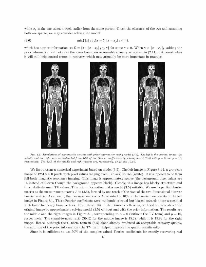
Fig. 3.1. Simulations of compressive sensing with prior information using model (3.5). The left is the original image, the

middle and the right were reconstructed from 10% of the Fourier coefficients by solving model (3.5) with µ = 0 and µ = 10,

respectively. The SNR of the middle and right images are, respectively, 15.28 and 19.89.

We first present a numerical experiment based on model (3.5). The left image in Figure 3.1 is a grayscale

image of 1281× 400 pixels with pixel values ranging from 0 (black) to 255 (white). It is supposed to be from

full-body magnetic resonance imaging. This image is approximately sparse (the background pixel values are

16 instead of 0 even though the background appears black). Clearly, this image has blocky structures and

thus relatively small TV values. This prior information makes model (3.5) suitable. We used a partial Fourier

matrix as the measurement matrix A in (3.5), formed by one tenth of the rows of the two-dimensional discrete

Fourier matrix. As a result, the measurement vector b consisted of 10% of the Fourier coefficients of the left

image in Figure 3.1. These Fourier coefficients were randomly selected but biased towards those associated

with lower frequency basis vectors. From these 10% of the Fourier coefficients, we tried to reconstruct the

original image by approximately solving model (3.5) without and with the prior information. The results are

the middle and the right images in Figure 3.1, corresponding to µ = 0 (without the TV term) and µ = 10,

respectively. The signal-to-noise ratio (SNR) for the middle image is 15.28, while it is 19.89 for the right

image. Hence, although the `1-norm term in (3.5) alone already produced an acceptable recovery quality,

the addition of the prior information (the TV term) helped improve the quality significantly.

Since it is sufficient to use 50% of the complex-valued Fourier coefficients for exactly recovering real

11

images, at least in theory, the use of 10% of the coefficients represents an 80% reduction in the amount of

data required for recovery. In fact, simulations in this example indicates how CS may be applied to MRI

where scanned data are essentially Fourier coefficients of images under construction. A 80% reduction in

MRI scanning time would represent a significant improvement in MRI practice. We refer the reader to the

work of Lustig, Donoho, Santos and Pauly [23], and the references therein, for more information on the

applications of CS to MRI.

The above example, however, does not show that prior information can actually reduce the number

of measurements required for recovery of sparse signals. For that purpose, we present another numerical

experiment based on model (3.6) with additional nonnegativity constraint.

We consider reconstructing a nonnegative, sparse signal x ∈ Rn from the measurement b = Ax with or

without the prior information that x is close to a known prior signal xp. The decoding models without and

with this prior information are, respectively,

(3.7) min‖x‖1 : Ax = b, x ≥ 0,(3.8) min‖x‖1 : Ax = b, x ≥ 0, ‖x− xp‖1 ≤ γ.

In our experiment, the signal length is fixed at n = 100, and the sparsity of both x and xp is k = 10. More

specifically, both x and xp have 10 nonzero elements of the value 1, but only 8 of the 10 nonzero positions

coincide while the other 2 nonzeros occur at different positions. Roughly speaking, there is a 20% difference

between x and xp. Obviously, ‖x− xp‖1 = 4.

0 10 20 30 400

10

20

30

40

50

60

70

80

90

100

Number of measurements

Perc

enta

ge

Recovery Rate

10 20 30 40

10

20

30

40

50

60

70

80

90

100

Number of measurements

Perc

enta

ge

Average Error

without prior

with prior

Fig. 3.2. Recovery rate (left) and average relative error (right) on 100 random problems with (solid line) and without

(dashed line) prior information. For fixed n = 100 and k = 10, the number of measurements m ranges from 2 to 40.

We ran both (3.7) and (3.8) on 100 random problems with the number of measurements m = 2, 4, · · · , 40,

where in each problem A ∈ Rm×n is a standard Gaussian random matrix, and the 10 nonzero positions of x

and xp are randomly chosen with 8 positions coinciding. In (3.8), we set γ = 4 which equals ‖x − xp‖1 by

construction. We regard a recovered signal to be “exact” if it has a relative error below 10−4. The numerical

results are presented in Figure 3.3 that gives the percentage of exact recovery and the average relative error

in `2-norm on 100 random trials for each m value.

We observe that without the prior information m = 40 was needed for 100-percent recovery, while with

the prior information m = 20 was enough. If we consider approximate recovery, we see that to achieve an

accuracy with relative errors below 10-percent, the required numbers of measurements were m = 30 and

m = 14, respectively, for models (3.7) and (3.8).

12

4. Stability. In practice, a measurement vector b is most likely inaccurate due to various sources of

imprecisions and/or contaminations. A more realistic measurement model should be b = Ax+ r where x is

a desirable and sparse signal, and r ∈ Rm can be interpreted either as noise or as spurious measurements

generated by a noise-like signal. Now given an under-sampled and imprecise measurement vector b = Ax+r,

can we still approximately recover the sparse signal x? What kind of errors should we expect? These are

questions our stability analysis should address.

4.1. Preliminaries. Assume that A ∈ Rm×n is of rank m and b = Ax + r, where x ∈ Ω ⊂ Rn. Since

the sparse signal of interest, x, does not necessarily satisfy the equation Ax = b, we relax our goal to the

inequality ‖Ax − b‖ ≤ γ in some norm ‖ · ‖, with γ ≥ ‖r‖ so that x satisfies the inequality. An alternative

interpretation for the imprecise measurement b is that it is generated by a signal x that is approximately

sparse so that b = Ax for x = x+ p where p is small and satisfies Ap = r.

Consider the QR-factorization: AT = UR, where U ∈ Rn×m satisfies UTU = I and R ∈ Rm×m is upper

triangular. Obviously, Ax = b is equivalent to UTx = R−T b, and

‖Ax− b‖M = ‖UTx−R−T b‖2,

where

(4.1) ‖q‖M = (qTMq)1/2 and M = (RTR)−1.

We will make use of the following two projection matrices:

(4.2) Pr = AT (AAT )−1A ≡ UUT and Pn = I − Pr,

where Pr is the projection onto the range space of AT and Pn onto the null space of A. In addition, we will

use the constant

(4.3) Cν =1 + ν

√2− ν2

1− ν2> 1, ν ∈ (0, 1).

It is easy to see that as ν approaches 1, Cν ≈ 1/(1− ν). For example, Cν ≈ 2.22 for ν = 0.5, Cν ≈ 4.34 for

ν = 0.75 and Cν ≈ 10.43 for ν = 0.9.

4.2. Two Stability Results. Given the imprecise measurement b = Ax + r, consider the decoding

model

(4.4) x∗γ = arg minx∈Ω

‖x‖1 : ‖Ax− b‖M ≤ γ = arg minx∈F(γ)

‖x‖1,

where Ω ⊂ Rn is a closed, prior-information set, γ ≥ ‖r‖2, the weighted norm is defined in (4.1), and

(4.5) F(γ) = x : ‖Ax− b‖M ≤ γ, x ∈ Ω.

In general, x∗γ 6= x and is not strictly sparse. We will show that x∗γ is close to x under suitable conditions.

To our knowledge, stability of this model has not been previously investigated. Our result below says that if

F(γ) contains a sufficiently sparse point x, then the distance between x∗γ and x is of order γ. Consequently,

If x ∈ F(0), then x∗0 = x.

The use of the weighted norm ‖ · ‖M in (4.4) is purely for convenience because it simplifies constants

involved in derived results. Had another norm been used, extra constants would appear in some derived

inequalities. Nevertheless, due to the equivalence of norms in Rm, the essence of those stability results

remains unchanged.

13

In our stability analysis below, we will make use of the following sparsity condition:

(4.6) k =ν2

4

(‖u‖1‖u‖2

)2

, for some ν ∈ (0, 1).

Theorem 4.1. Let γ ≥ ‖Ax − b‖M for some x ∈ Ω. Assume that k = ‖x‖0 satisfies (4.6) for

u = Pn(x∗γ − x) whenever Pn(x∗γ − x) 6= 0. Then for p = 1 or 2

(4.7) ‖x∗γ − x‖p ≤ γp(Cν + 1)(‖Ax− b‖M + γ),

where γ1 =√n, γ2 = 1 and Cν is defined in (4.3).

Remark 4. We quickly add that if A is a standard normal random matrix, then the KGG inequality

(3.3) implies that with high probability the right-hand side of (4.6) for u = Pn(x∗γ − x) is at least of the order

m/ log(n/m). This same comment also applies to the next theorem.

The proof of this theorem, as well as that of Theorem 4.2 below, will be given in Subsection 4.4. Next

we consider the special case γ = 0, namely,

x∗0 = arg minx∈Ω

‖x‖1 : Ax = b.

A k-term approximation of x ∈ Rn, denoted by x(k), is obtained from x by setting its n − k smallest

elements in magnitude to zero. Obviously, ‖x‖1 ≡ ‖x(k)‖1 + ‖x− x(k)‖1. Due to measurement errors, there

may be no sparse signal that satisfies the equation Ax = b. In this case, we show that if the observation b

is generated by a signal x that has a good, k-term approximation x(k), then the distance between x∗0 and x

is bounded by the error in the k-term approximation. Consequently, if x is itself k-sparse so that x = x(k),

then x∗0 = x.

Theorem 4.2. Let x ∈ Ω satisfy Ax = b and x(k) be a k-term approximation of x. Assume that k

satisfies

(4.8) ‖x− x(k)‖1 ≤ ‖x‖1 − ‖x∗0‖1

and (4.6) for u = Pn(x∗0 − x(k)) whenever Pn(x∗0 − x(k)) 6= 0. Then for p = 1 or 2

(4.9) ‖x∗0 − x(k)‖p ≤ (Cν + 1)‖Pr(x− x(k))‖p,

where Cν is defined in (4.3).

It follows from (4.9) and the triangle inequality that for p = 1 or 2

(4.10) ‖x∗0 − x‖p ≤ (Cν + 1)‖Pr(x− x(k))‖p + ‖x− x(k)‖p,

which has the same type of left-hand side as those in (1.4) and (1.5).

Condition (4.8) can always be met for k sufficiently large, while condition (4.6) demands that k be

sufficiently small. Together, the two require that the measurement b be observed from a signal x that has a

sufficiently good k-term approximation for a sufficiently small k. This requirement seems very reasonable.

4.3. Comparison to RIP-based Stability Results. In the special case of Ω = Rn, the error bounds

in Theorems 4.1 and 4.2 bear similarities with existing stability results by Candes, Romberg and Tao [7] (see

(1.4)–(1.6) in Section 1 and also results in [10]), but substantial differences exist in the constants involved

and the conditions required. Overall, Theorems 4.1 and 4.2 do not contain, nor are contained in, the existing

results, though they all state the same fact that CS recovery based on `1-minimization is stable to some

extent.

14

The main differences between the RIP-based stability results and ours are reflected in the constants

involved. In our error bound (4.9) the constant is given by a formula depending only on the number ν ∈ (0, 1)

representing the sparsity level of the signal under construction relative to a maximal recoverable sparsity

level. The sparser the signal is, the smaller the constant is, and the more stable the recovery is supposed to

be. However, the maximal recoverable sparsity level does depend on the null space of a measurement matrix

even though it is independent of matrix representations of that space (hence independent of nonsingular row

transformations).

This is not the case, however, with the RIP-based stability results where the involved constants depend

on RIP parameters of matrix representations. The smaller the RIP parameters, the smaller those constants.

As has been discussed in Section 1.3, any RIP-based result, be it recoverability or stability, will unfortu-

nately break down under nonsingular row transformation, even though the decoding model (1.10) itself is

mathematically invariant of such a transformation.

Given the monotonicity of the involved stability constants, the key difference between RIP-free and

RIP-based stability results can be summarized as follows. For a fixed row space, the former suggests that

the sparser is the signal, the more stable; while the latter suggests that the better conditioned is a matrix

representation for the row subspace, the more stable. Mathematically, the latter characterization is obviously

misleading.

Theorem 4.2 requires a side condition (4.8), which is not required by RIP-based results. We can argue

that this side condition is not restrictive because stability results such as (4.9) are only meaningful when

the bound on the right-hand side is small; otherwise, the solution errors in the left-hand side would be out

of control. Nevertheless, the RIP-free stability result in (4.9) has recently been strengthened by Vavasis [30]

who shows that the side condition (4.8) can be removed in the `1-norm case.

4.4. Proofs of Our Stability Results. Our stability results follow directly from the following simple

lemma.

Lemma 4.3. Let x, y ∈ Rn such that ‖y‖1 ≤ ‖x‖1, and let y − x = u + w. where uTw = 0. Whenever

u 6= 0, assume that k = ‖x‖0 satisfies (4.6). Then for either p = 1 or p = 2, there hold

(4.11) ‖u‖p ≤ Cν‖w‖p,

and

(4.12) ‖y − x‖p ≤ (Cν + 1)‖w‖p.

Proof. If u = 0, both (4.11) and (4.12) are trivially true. If u 6= 0, condition (4.6) and the assumption

‖y‖1 ≤ ‖x‖1 imply that w 6= 0; otherwise, by Lemma 2.1, (4.6) would imply ‖y‖1 > ‖x‖1. For u 6= 0 and

w 6= 0,

‖u+ w‖1‖u+ w‖2

≥

(1− ‖w‖1/‖u‖1√1 + (‖w‖2/‖u‖2)2

)‖u‖1‖u‖2

,

which follows from the triangle inequality ‖u+ w‖1 ≥ ‖u‖1 − ‖w‖1. Furthermore,

(4.13)‖u+ w‖1‖u+ w‖2

≥

(1− η(u,w)√1 + η(u,w)2

)‖u‖1‖u‖2

, φ(η(u,w))‖u‖1‖u‖2

,

where φ(t) = (1− t)/√

1 + t2 and

(4.14) η(u,w) , max

‖w‖1‖u‖1

,‖w‖2‖u‖2

.

15

If 1− η(u,w) ≤ 0, then (4.11) trivially holds. Therefore, we assume that η(u,w) < 1.

If φ(η(u,w)) > ν, then it follows from (4.6) and (4.13) that

√‖x‖0 ≤

ν

2

‖u‖1‖u‖2

≤ ν/φ(η(u,w))

2

‖u+ w‖1‖u+ w‖2

<1

2

‖u+ w‖1‖u+ w‖2

,

which would imply ‖x‖1 < ‖y‖1 by Lemma 2.1, contradicting the assumption of the lemma. Therefore,

φ(η(u,w)) ≤ ν must hold. It is easy to verify that

φ(t) =1− t√1 + t2

≤ ν and t < 1 ⇐⇒ 1

Cν≤ t < 1,

where 1/Cν is the root of the quadratic q(t) , (1−t)2−ν2(1+t2) that is smaller than 1 (noting that φ(t) ≤ νis equivalent to q(t) ≤ 0 for t < 1). We conclude that there must hold η(u,w) ≥ 1/Cν , which implies (4.11) in

view of the definition of η(u,w) in (4.14). Finally, (4.12) follows directly from the relationship y−x = u+w,

the triangle inequality, and (4.11).

Clearly, whether the estimates of the lemma hold for p = 1 or p = 2 depends on which ratio is larger

in (4.14); or equivalently, which ratio is larger between ‖u‖1/‖u‖2 and ‖w‖1/‖w‖2. If u is from a random,

(n−m)-dimensional subspace of Rn, then w is from its orthogonal complement — a random, m-dimensional

subspace. When n−m m, the KGG result indicates that it is more likely that ‖u‖1/‖u‖2 < ‖w‖1/‖w‖2;

or equivalently, ‖w‖2/‖u‖2 < ‖w‖1/‖u‖1. In this case, p = 1 is more likely than p = 2.

Corollary 4.4. Let U ∈ Rn×m with m < n have orthonormal columns so that UTU = I. Let x, y ∈ Rn

satisfy ‖y‖1 ≤ ‖x‖1 and ‖UT y−d‖2 ≤ γ for some d ∈ Rm. Define u , (I−UUT )(y−x) and w , UUT (y−x).

In addition, let k = ‖x‖0 satisfy (4.6) whenever u 6= 0. Then

(4.15) ‖y − x‖p ≤ γp(Cν + 1)(‖UTx− d‖2 + γ), p = 1 or 2,

where γ1 =√n and γ2 = 1.

Proof. Noting that y = x+ u+ w and UTu = 0, we calculate

γ ≥ ‖UT (x+ u+ w)− d‖2 = ‖UTw − (d− UTx)‖2 ≥ ‖UTw‖2 − ‖UTx− d‖2,

which implies

(4.16) ‖w‖2 = ‖UTw‖2 ≤ γ + ‖UTx− d‖2.

Combining (4.16) with (4.12), we arrive at (4.15) for either p = 1 or 2, where in the case of p = 1 we use the

inequality ‖w‖1 ≤√n‖w‖2.

Proof of Theorem 4.1

Proof. Since x ∈ F(γ) and x∗γ minimizes the 1-norm in F(γ), we have ‖x∗γ‖1 ≤ ‖x‖1. The proof then

follows from applying Corollary 4.4 to y = x∗γ and x = x, and the fact that the weighted norm defined in

(4.1) satisfies ‖Ax− b‖M = ‖UTx−R−T b‖2.

Proof of Theorem 4.2

Proof. We note that condition (4.8) is equivalent to ‖x∗0‖1 ≤ ‖x(k)‖1 since ‖x‖1 = ‖x− x(k)‖1 +‖x(k)‖1.

Upon applying Lemma 4.3 to y = x∗0 and x = x(k) with u = Pn(y − x) and w = Pr(y − x), and also noting

Prx∗0 = Prx, we have

‖x∗0 − x(k)‖p ≤ (Cν + 1)‖Pr(x(k)− x)‖p,

which completes the proof.

16

5. Uniform Recoverability. The recoverability result, Theorem 3.2, is derived essentially only for

standard normal random matrices. It has been empirically observed (see [15, 16], for example) that recov-

ery behavior of many different random matrices seems to be identical. We call this phenomenon uniform

recoverability. In this section, we provide a theoretical explanation to this property.

5.1. Preliminaries. We will consider the simple case where Ω = Rn and γ = 0 so that we can make use

of the necessary and sufficient condition in Proposition 2.3. We first translate this necessary and sufficient

condition into a form more conducive to our analysis.

For 0 < k < n, we define the following function that maps a vector in Rn to a scalar:

(5.1) λk(v) ,‖v‖1 − 2‖v(k)‖1

‖v‖2, v 6= 0,

where v(k) is a k-term approximation of v whose nonzero elements are the k largest elements of v in

magnitude. It is important to note that λk(v) is invariant with respect to multiplications by scalars (or scale-

invariant) and permutations of v. Moreover, λk(v) is continuous, and achieves its minimum and maximum

(since its domain can be restricted to the unit sphere).

Proposition 5.1. Given A ∈ Rm×n with m < n, the equivalence (2.12), i.e.,

x = arg min‖x‖1 : Ax = Ax,

holds for all x with ‖x‖0 ≤ k if and only if

(5.2) 0 < Λk(A) , minλk(v) : v ∈ N (A) \ 0.

Proof. For any fixed v 6= 0, the condition ‖v‖1 > 2‖vα‖1 in (2.13) for all index sets α with |α| ≤ k is

clearly equivalent to λk(v) > 0. After taking the minimum over all v 6= 0 in N (A), we see that Λk(A) > 0

is equivalent to the necessary and sufficient condition in Proposition 2.3.

For notational convenience, given any A ∈ Rm×n with m < n, let us define the set

sub(A) =B ∈ Rm×(m+1) : B is a submatrix of A

.

In other words, each member of sub(A) is formed by m + 1 columns of A in their original order. Clearly,

the cardinality of sub(A) is n choose m + 1. We say that the set sub(A) has full rank if every member

of sub(A) has rank m. It is well known that for most distributions, sub(A) will have full rank with high

probability.

5.2. Results for Uniform Recoverability. When A ∈ Rm×n is randomly chosen from a probability

space, Λk(A) is a random variable whose sign, according to Proposition 5.1, determines the success or failure

of recovery for all x with ‖x‖0 ≤ k. In this setting, the following theorem indicates that Λk(A) is a sample

minimum of another random variable λk(d(B)) where B ∈ Rm×(m+1) is from the same probability space as

A, and d(B) ∈ Rm+1 is defined by

(5.3) [d(B)]i , |det(Bi)|, i = 1, · · · ,m+ 1,

where Bi ∈ Rm×m is the submatrix of B obtained by deleting the i-th column of B.

Theorem 5.2. Let A ∈ Rm×n (m < n) with sub(A) of full rank (i.e., every member of sub(A) has

rank m). Then for k ≤ m

(5.4) Λk(A) = min λk(d(B)) : B ∈ sub(A) ,17

where d(B) ∈ Rm+1 is defined in (5.3).

The proof of this theorem is left to Subsection 5.4.

Remark 5. Theorem 5.2, together with Proposition 5.1, establishes that recoverability is determined by

the properties of d(B), not directly those of A. If distributions of d(B) for different types of random matrices

converge to the same limit as m→∞, then asymptotically there should be an identical recovery behavior for

different types of random matrices.

For any random matrix B, by definition the components of d(B) are random determinants (in absolute

value). It has been established by Girko [18] that a wide class of random determinants (in absolute value)

does share a limit distribution (see the book by Girko [19] for earlier results).

Theorem 5.3 (Girko). For any m, let the random elements t(m)ij , 1 ≤ i, j ≤ m, of the matrix Tm = [t

(m)ij ]

be independent, E(t(m)ij ) = µ, Var(t

(m)ij ) = 1 and supi,j,m E|t(m)

ij |4+δ <∞ for some δ > 0. Then

(5.5) limm→∞

Prob

log(det(Tm)2/[(m− 1)!(1 +mµ2)]

)√

2 logm< t

=

1√2π

∫ t

−∞e−

x2

2 dx.

Theorem 5.3 says that for a wide class of random determinants squared, their logarithms, with proper

scalings, converge in distribution to the standard normal law; or the limit distribution of the random deter-

minants squared is log-normal.

Remark 6. Since the elements of d(B) are random determinants in absolute value, they all have the

same limit distribution as long as B satisfies the conditions of Theorem 5.3.

The elements of d(B) are not independent in limit, because any two of them are determinants of m×mmatrices that share m − 1 common columns. However, the cause of such dependency among elements of

d(B) is purely algebraic, and hence does not vary with the type of random matrices. To stress this point,

we mention that for a wide range of random matrices B, the ratios det(Bi)/det(Bj), i 6= j, converge to

Cauchy distribution with the cumulative distribution function 1/2 + arctan(t)/π. This result can be found,

in a slightly different form, in Theorem 15.1.1 of the book by Girko [19].

Remark 7. We observe from (5.5) that the mean values µ only affect the scaling factor of the determi-

nant, but not the asymptotic recoverability behavior since λk(·) is scale-invariant, implying that measurement

matrices need not have zero mean, as is usually required in earlier theoretical results of this sort. In addition,

the unit variance assumption in Theorem 5.3 is not restrictive because it can always be achieved by scaling.

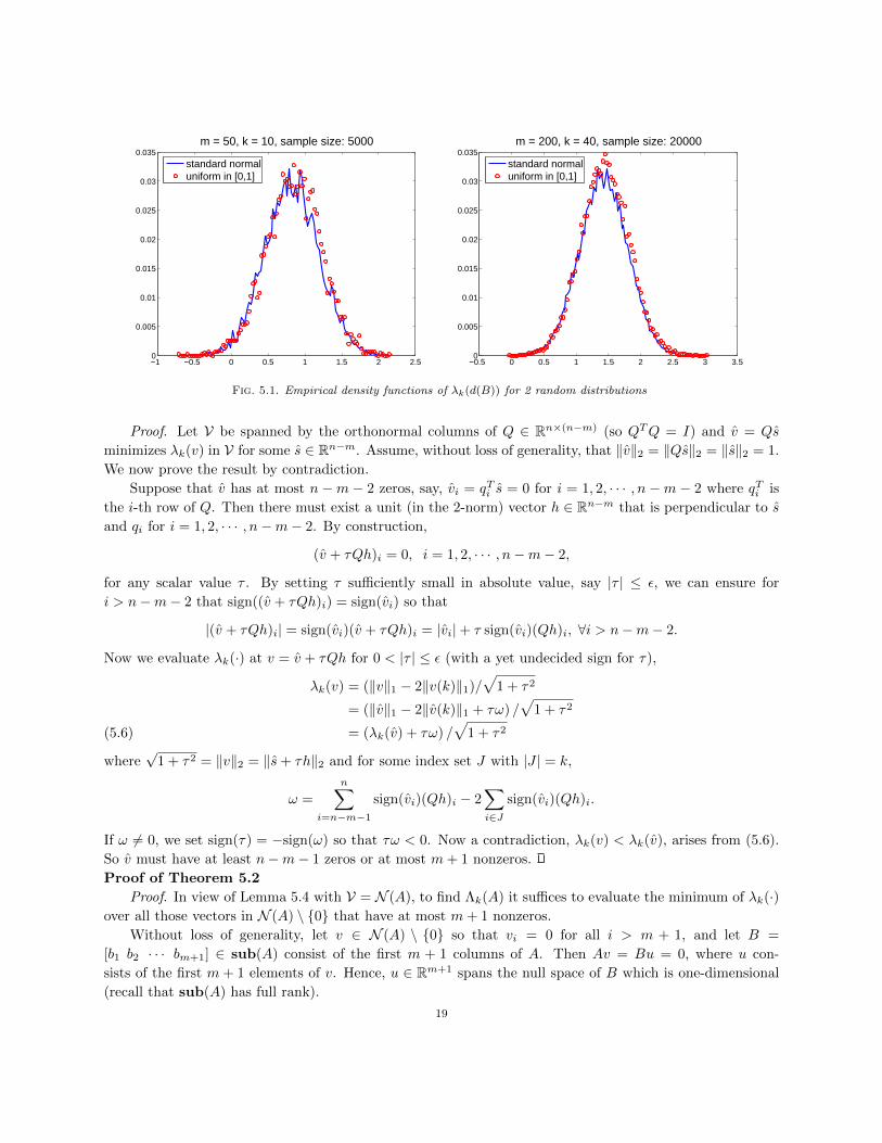
5.3. Numerical Illustration. To illustrate the uniformity of CS recovery, we sample the random vari-

able λk(d(B)) for B ∈ Rm×(m+1) whose entries are iid and randomly drawn from one of the two probability

distributions: the standard normal distribution N (0, 1) or the uniform distribution on the interval [0, 1].

While the former has zero mean, the latter has mean 1/2. In Figure 5.1, we plot the empirical density

functions (namely, scaled histograms) of λk(d(B)) for the two random distributions with different values of

m, k and sample size. Recall that successful recovery of all k-sparse signals is guaranteed for matrix A if

and only if the sample minimum of λk(d(B)) over sub(A) is positive.

As can be seen from Figure 5.1, even at m = 50, the two empirical density functions for λ10(d(B)),

corresponding to the standard normal (solid line) and the uniform distributions (small circles) respectively,

are already fairly close. At m = 200, the two empirical density functions for λ40(d(B)) become largely

indistinguishable in most places.

5.4. Proof of Theorem 5.2. The following result, established by Eydelzon [16] in a slightly different

form, will play a key role in the proof. For completeness, we include a proof for it.

Lemma 5.4. Let V be an (n − m)-dimensional subspace of Rn and k ≤ m < n. If v ∈ V minimizes

λk(v) in V, then v has at least n−m− 1 zeros, or equivalently at most m+ 1 nonzeros.

18

−1 −0.5 0 0.5 1 1.5 2 2.50

0.005

0.01

0.015

0.02

0.025

0.03

0.035m = 50, k = 10, sample size: 5000

standard normaluniform in [0,1]

−0.5 0 0.5 1 1.5 2 2.5 3 3.50

0.005

0.01

0.015

0.02

0.025

0.03

0.035m = 200, k = 40, sample size: 20000

standard normaluniform in [0,1]

Fig. 5.1. Empirical density functions of λk(d(B)) for 2 random distributions

Proof. Let V be spanned by the orthonormal columns of Q ∈ Rn×(n−m) (so QTQ = I) and v = Qs

minimizes λk(v) in V for some s ∈ Rn−m. Assume, without loss of generality, that ‖v‖2 = ‖Qs‖2 = ‖s‖2 = 1.

We now prove the result by contradiction.

Suppose that v has at most n −m − 2 zeros, say, vi = qTi s = 0 for i = 1, 2, · · · , n −m − 2 where qTi is

the i-th row of Q. Then there must exist a unit (in the 2-norm) vector h ∈ Rn−m that is perpendicular to s

and qi for i = 1, 2, · · · , n−m− 2. By construction,

(v + τQh)i = 0, i = 1, 2, · · · , n−m− 2,

for any scalar value τ . By setting τ sufficiently small in absolute value, say |τ | ≤ ε, we can ensure for

i > n−m− 2 that sign((v + τQh)i) = sign(vi) so that

|(v + τQh)i| = sign(vi)(v + τQh)i = |vi|+ τ sign(vi)(Qh)i, ∀i > n−m− 2.

Now we evaluate λk(·) at v = v + τQh for 0 < |τ | ≤ ε (with a yet undecided sign for τ),

λk(v) = (‖v‖1 − 2‖v(k)‖1)/√

1 + τ2

= (‖v‖1 − 2‖v(k)‖1 + τω) /√

1 + τ2

= (λk(v) + τω) /√

1 + τ2(5.6)

where√

1 + τ2 = ‖v‖2 = ‖s+ τh‖2 and for some index set J with |J | = k,

ω =

n∑i=n−m−1

sign(vi)(Qh)i − 2∑i∈J

sign(vi)(Qh)i.

If ω 6= 0, we set sign(τ) = −sign(ω) so that τω < 0. Now a contradiction, λk(v) < λk(v), arises from (5.6).

So v must have at least n−m− 1 zeros or at most m+ 1 nonzeros.

Proof of Theorem 5.2

Proof. In view of Lemma 5.4 with V = N (A), to find Λk(A) it suffices to evaluate the minimum of λk(·)over all those vectors in N (A) \ 0 that have at most m+ 1 nonzeros.

Without loss of generality, let v ∈ N (A) \ 0 so that vi = 0 for all i > m + 1, and let B =

[b1 b2 · · · bm+1] ∈ sub(A) consist of the first m + 1 columns of A. Then Av = Bu = 0, where u con-

sists of the first m+ 1 elements of v. Hence, u ∈ Rm+1 spans the null space of B which is one-dimensional

(recall that sub(A) has full rank).

19

Let Bi be the submatrix of B with its i-th column removed. Without loss of generality, we assume that

det(B1) 6= 0. Clearly, the null space of B is spanned by the vector

u =

(−1

B−11 b1

)∈ Rm+1,

where, by Crammer’s rule, (B−11 b1)i = det(Bi+1)/ det(B1), i = 1, 2, · · · ,m. Since the function λk(·) is

scale-invariant, to evaluate λk(·) at v ∈ N (A) \ 0 with vi = 0 for i > m + 1, it suffices to evaluate it at

d(B) , |det(B1)u|, which coincides with the definition in (5.3).

Obviously, the exactly same argument can be equally applied to all other nonzero vectors in N (A) which

have at most m + 1 nonzeros in different locations, corresponding to different members of sub(A). This

completes the proof.

6. Conclusions. CS is an emerging methodology with a solid theoretical foundation that is still evolv-

ing. Most previous analyses in the CS theory relied on the RIP of the measurement matrix A. These analyses

can be called matrix-based. The non-RIP analysis presented in this paper, however, is subspace-based, and

utilizes the classic KGG inequality to supply the order of recoverable sparsity. It should be clear from this

non-RIP analysis that CS recoverability and stability, when using the equation Ax = b, are solely determined

by the properties of the subspaces associated with A regardless of matrix representations.

The non-RIP approach used in this paper has enabled us to derive the extended recoverability and

stability results immediately from a couple of remarkably simple observations (Lemmas 2.1 and 4.3) on the

2-norm versus 1-norm ratio in the null space of A. The obtained extensions include: (a) allowing the use of

prior information in recovery, (b) establishing RIP-free formulas for stability constants, and (c) explaining

the uniform recoverability phenomenon. In our view, these new results reinforce the theoretical advantages

of `1-minimization-based CS decoding models.

As has been alluded to at the beginning, there are topics in the CS theory that are not covered in this

work, one of which is that the recoverable sparsity order given in Theorem 3.2 can be shown to be optimal in

a sense (see [4] for an argument). Nevertheless, it is hoped that this work will help enhance and enrich the

theory of CS, make the theory more accessible, and stimulate more activities in utilizing prior information

and different measurement matrices in CS research and practice.

Acknowledgments. The author is grateful to two anonymous referees for their valuable comments

and suggestions that have helped improve the paper. The author’s appreciation also goes to Mark Ebmree,

Junfeng Yang and Wotao Yin for their reading of earlier drafts of the paper and many useful comments and

suggestions. The work of the author has been supported in part by NSF Grant DMS-0811188 and ONR

Grant N00014-08-1-1101.

REFERENCES

[1] R. Baraniuk, M. Davenport, R. DeVore and M. Wakin. A simple proof of the restricted isometry property for random

matrices. To appear in Constructive Approximation. 2007.

[2] A. Barvinok. Math 710: Measure Concentration. Lecture notes, Department of Mathematics, University of Michigan,

Ann Arbor, Michigan 48109-1109.

[3] E. Candes. The restricted isometry property and its implications for compressed sensing. Comptes Rendus Mathematique,

Vol. 346, pp. 589 - 592, 2008.

[4] E. Candes. Compressive sampling. International Congress of Mathematicians, Madrid, Spain, August 22-30, 2006 (Eur.

Math. Soc., Zurich, 2006), Vol. 3, pp. 1433-1452.

[5] E. Candes and T. Tao. Near optimal signal recovery from random projections: universal encoding strategies. IEEE

Transactions on Information Theory, 52 (2006), pp. 5406–5425.

[6] E. Candes and T. Tao. Decoding by linear programming. IEEE Transactions on Information Theory, Vol. 51, pp.

4203–4215, 2005.

20

[7] E. Candes, J. Romberg, and T. Tao, Stable signal recovery from incomplete and inaccurate information. Communications

on Pure and Applied Mathematics, 2005 (2005), pp. 1207–1233.

[8] E. Candes, J. Romberg, and T. Tao, Robust uncertainty principles: exact signal reconstruction from highly incomplete

frequency information. IEEE Trans. Inform. Theory 52 (2006), 489–509.

[9] S. S. Chen, D. L. Donoho, and M. A. Saunders. Atomic decomposition by basis pursuit. SIAM J. Scientific Computing

20: 33-61, 1998.

[10] A. Cohen, W. Dahmen, and R. A. DeVore. Compressed sensing and k-term approximation. Submitted., (2007).

[11] D. Donoho. Compressed sensing. IEEE Transactions on Information Theory, 52 (2006), pp. 1289–1306.

[12] D. Donoho and M. Elad. Optimally sparse representation in general (nonorthogonal) dictionaries via `1 minimization.

Proc. Natl. Acad. Sci. U.S.A., 100(2003): 2197–2202.

[13] D. Donoho and J. Tanner. Counting faces of randomly-projected polytopes when the projection radically lowers dimension.

Submitted to Journal of the AMS, (2005).

[14] D. Donoho and J. Tanner. Sparse Nonnegative Solutions of Underdetermined Linear Equations by Linear Programming.

Proceedings of the National Academy of Sciences (USA), 2005 v102(27): 9446-9451.

[15] D. Donoho and Y. Tsaig. Extensions of compressed sensing. Signal Processing, 86(3), pp. 533-548, March 2006.

[16] Anatoly Eydelzon. A Study on Conditions for Sparse Solution Recovery in Compressive Sensing. PhD Thesis, Rice

University, CAAM Technical Report TR07-12, (2007).

[17] A. Garnaev and E. D. Gluskin. The widths of a Euclidean ball. Dokl. Akad. Nauk SSSR, 277 (1984), pp. 1048–1052.

[18] V. L. Girko. A Refinement of the Central Limit Theorem for Random Determinants. Theory of Probability and its

Applications. Vol. 42, No. 1, pp. 21-129. 1998, (translated from a Russian Journal).

[19] V. L. Girko. Theory of Random Determinants. Kluwer Academic Publishers, Dordrecht, Boston, London. 1990.

[20] E. Gluskin and V. Milman. Note on the Geometric-Arithmetic Mean Inequality. Geometric Aspects of Functional Analysis

Israel Seminar 2001-2002. Lecture Notes in Mathematics, Springer, Berlin, Heidelberg. Vol.1807/2003, pp.131 - 135.

[21] B. S. Kashin. Diameters of certain finite-dimensional sets in classes of smooth functions. Izv. Akad. Nauk SSSR, Ser.

Mat., 41 (1977), pp. 334–351.

[22] B. S. Kashin and V. N. Temlyakov. A Remark on Compressed Sensing. Mathematical Notes, 2007, Vol. 82, No. 6, pp.

748–755. Pleiades Publishing, Ltd., 2007.

[23] M. Lustig, D. Donoho, J. Santos and J. Pauly. Compressed Sensing MRI. IEEE Signal Processing Magazine, March

(2008): 72–82.

[24] V. D. Milman and G. Schechtman. Asymptotic Theory of Finite Dimensional Normed Spaces, With an Appendix by M.

Gromov. Lecture Notes in Mathematics 1200. Springer, (2001).

[25] D. Needell and J. A. Tropp. CoSaMP: Iterative signal recovery from incomplete and inaccurate samples. arXiv:0803.2392v2,

2008.

[26] D. Needell and R. Vershynin. Signal recovery from incomplete and inaccurate measurements via regularized orthogonal

matching pursuit. Submitted for publication, October 2007.

[27] M. Rudelson and R. Vershynin. Geometric approach to error correcting codes and reconstruction of signals. International

Mathematical Research Notices, 64 (2005), pp. 4019–4041.

[28] F. Santosa and W. Symes. Linear inversion of band-limited reflection histograms. SIAM Journal on Scientific and

Statistical Computing. 7 (1986), pp. 1307–1330.

[29] J. A. Tropp and A. C. Gilbert. Signal recovery from random measurements via orthogonal matching pursuit. IEEE Trans.

Info. Theory, 53(12): 4655–4666, 2007.

[30] S. Vavasis. Derivation of compressive sensing theorems for the spherical section property. University of Waterloo, CO 769

lecture notes. 2009.

[31] Y. Zhang. A Simple Proof for Recoverability of `1-Minimization: Go Over or Under? Rice University CAAM Technical

Report TR05-09, (2005).

[32] Y. Zhang. A Simple Proof for Recoverability of `1-Minimization (II): the Nonnegativity Case. Rice University CAAM

Technical Report TR05-10, (2005).

[33] Compressive Sensing Resources. http://www.dsp.ece.rice.edu/cs.

21