theory and applications of coupling based intensity modulated fibre …117472/fulltext… · ·...
TRANSCRIPT

Thesis for the degree of Licentiate of Technology
Sundsvall 2008
Theory and Applications of Coupling Based
Intensity Modulated Fibre-Optic Sensors
Johan Jason
Supervisors: Prof. Hans-Erik Nilsson
Dr. Bertil Arvidsson
Electronics Design Division,
Department of Information Technology and Media
Mid Sweden University, SE-851 70 Sundsvall, Sweden
ISSN 1652-8948
Mid Sweden University Licentiate Thesis 35
ISBN 978-91-86073-20-6
Akademisk avhandling som med tillstånd av Mittuniversitetet i Sundsvall
framläggs till offentlig granskning för avläggande av licentiatexamen i elektronik
onsdagen den 17 december 2008, klockan 13.15 i sal O111, Mittuniversitetet
Sundsvall. Seminariet kommer att hållas på engelska.
Theory and Applications of Coupling Based
Intensity Modulated Fibre-Optic Sensors
Johan Jason
© Johan Jason, 2008
Electronics Design Division,
Department of Information Technology and Media
Mid Sweden University, SE-851 70 Sundsvall
Sweden
Telephone: +46 (0)771 975000
Printed by Kopieringen Mittuniversitetet, Sundsvall, Sweden, 2008

For Johanna, Sigrid, Helga and Alfred


i
ABSTRACT
Optical fibre sensors can be used to measure a wide variety of properties. In some
cases they have replaced conventional electronic sensors due to their possibility of
performing measurements in environments suffering from electromagnetic
disturbance, or in harsh environments where electronics cannot survive. In other
cases they have had less success mainly due to the higher cost involved in fibre-
optic sensor systems.
Intensity modulated fibre-optic sensors normally require only low-cost monitoring
systems principally based on light emitting diodes and photo diodes. The sensor
principle itself is very simple when based on coupling between fibres, and coupling
based intensity modulated sensors have found applications over a long time, mainly
within position and vibration sensing.
In this thesis new concepts and applications for intensity modulated fibre-optic
sensors based on coupling between fibres are presented. From a low-cost and
standard component perspective alternative designs are proposed and analyzed in
order to find improved performance. The development of a sensor for an industrial
temperature sensing application, involving aspects on multiplexing and fibre
network installation, is presented. Optical time domain reflectometry (OTDR) is
suggested as an efficient technique for multiplexing several coupling based
sensors, and sensor network installation with blown fibre in micro ducts is
proposed as a flexible and cost-efficient alternative to traditional cabling.
A new sensor configuration using a fibre to a multicore fibre coupling and an
image sensor readout system is proposed. With this system a high-performance
sensor setup with a large measurement range can be realised without the need for
precise fibre alignment often needed in coupling based sensors involving fibres
with small cores. The system performance is analyzed theoretically with complete
system simulations on different setups. An experimental setup is made based on
standard fibre and image acquisition components, and differences from the
theoretical performance are analyzed. It is shown that sub-µm accuracy should be
possible to obtain, being the theoretical limit, and it is further suggested that the
experimental performance is mainly related to two error sources: core position
instability and differences between the real and the expected optical power
distribution. Methods to minimize the experimental error are proposed and
evaluated.


iii
SAMMANDRAG
Fiberoptiska sensorer kan användas för mätning av en rad olika parametrar. I
somliga fall har de ersatt konventionella elektroniska sensorer på grund av sin
förmåga att fungera i elektromagnetiskt störda miljöer, eller i andra besvärliga
miljöer där elektronik inte klarar sig. I andra fall har de haft mindre framgång
huvudsakligen på grund av att fiberoptiska sensorsystem oftast innebär en större
kostnad än konventionella system.
Intensitetsmodulerade fiberoptiska sensorer kräver normalt endast billiga
övervakningssystem i grunden baserade på lysdioder och fotodioder. Principen för
sådana sensorer baserade på koppling mellan fibrer är i sig själv mycket enkel, och
kopplingsbaserade intensitetsmodulerade fiberoptiska sensorer har haft
tillämpningar under en lång tid, huvudsakligen inom positions- och
vibrationsmätning.
I denna avhandling presenteras nya koncept och applikationer för
kopplingsbaserade intensitetsmodulerade fiberoptiska sensorer. Från ett
lågkostnads- och standardkomponentperspektiv föreslås och analyseras alternativa
lösningar för förbättrad prestanda. Utvecklingen av en sensor för
temperaturmätning i en industriell tillämpning, inbegripet aspekter på
sensormultiplexering och nätverksbyggande, behandlas. Optisk tidsdomän-
reflektometri (OTDR) presenteras som en effektiv teknik för multiplexering av
flera kopplingsbaserade sensorer, och installation av sensornätverk genom
användande av blåsfiberteknik och mikrodukter föreslås som ett flexibelt och
kostnadseffektivt alternativ till traditionell kabeldragning.
Ett nytt sensorkoncept baserat på koppling mellan en fiber och en
multikärnefiber/fiberarray och med ett bildsensorsystem för detektering föreslås.
Med denna konfiguration kan ett högpresterande sensorsystem med ett stort
mätområde åstadkommas utan behov av precis fiberupplinjering som annars ofta är
fallet för kopplingsbaserade sensorer med standardfiber. Systemets prestanda har
analyserats teoretiskt med kompletta systemsimuleringar för olika uppställningar.
En experimentell uppställning baserad på standardfiber och en kamera av
standardtyp har gjorts, och skillnader mellan experiment och simuleringar har
analyserats. Det visas att ett positionsbestämningsfel på mindre än 1 µm är
teoretiskt möjligt, och det antyds vidare att det experimentella resultatet
huvudsakligen är relaterat till två felkällor: instabilitet i kärnpositionerna hos
fiberarrayen samt skillnader mellan den verkliga och den förväntade optiska
effektfördelningen. Metoder för att minimera det experimentella felet föreslås och
analyseras.


v
ACKNOWLEDGEMENTS
First of all I want to thank my supervisors Hans-Erik Nilsson and Bertil Arvidsson
for the support behind this thesis. Hans-Erik, for clearly pointing out the important,
basic principles in research methodology, and for giving this project a new
dimension by suggesting an image sensor based detection system. Bertil, for giving
me the opportunity to enter deeply into different aspects of fibre-optic
measurements during my years at Ericsson. Thanks also to my mentor Anders
Larsson at Fiberson AB, who came with the suggestion to start this project.
I also want to thank all those who have taken part in, or in other ways contributed
to, the work in this thesis. Many thanks to Bengt Lindström and Håkan Olsson for
kindly lending me some of the equipment needed for the measurements, Pär Flöjt
for clever fibre preparation tricks, Arne Andersson for instructions on MT-
termination of fibre ribbons and Lars Andersson with staff at Ericsson for use of
termination equipment. Thanks to my colleagues at Fiberson AB for support in
different ways, especially Fredrik Sunnegårdh for help with software routines for
image acquisition and micropositioner control, Stefan Gistvik for graphical input
and Niklas Paulsson for fibre installation. The input from people at Iggesund
Paperboard AB, in particular Jan Söderberg, Jan Hellström and Melker Öberg, is
highly appreciated. Special thanks also to Prof. Jose Miguel López-Higuera and Dr.
Adolfo Cobo of the Photonics Engineering Group at Universidad de Cantabria, and
to Dr. Tarja Volotinen, for various technical discussions.
Further I would like to thank all the people at the Electronics Design Division at
Mid Sweden University, for creating such a friendly working environment, making
me feel at home although I had most of my research at the company. Special thanks
to Henrik Andersson and Anatoliy Manuilskiy for assistance in the customization
of the image sensor, and Andreas Ericsson for introduction to the camera control
commands. Thanks also to Fanny Burman for help with travel issues and other
practical things.
KK-stiftelsen (The Knowledge Foundation) is acknowledged for financial support.
My deepest thanks go to my wife Johanna for all your love and support, and to our
children Sigrid, Helga and Alfred for the joy you bring and for cheering me up
especially those days when research can be something of a pain rather than just
pure pleasure.
Hudiksvall/Sundsvall, 10 November 2008


vii
TABLE OF CONTENTS
ABSTRACT ............................................................................................................. I
SAMMANDRAG ................................................................................................. III
ACKNOWLEDGEMENTS .................................................................................. V
TABLE OF CONTENTS ................................................................................... VII
ABBREVIATIONS AND ACRONYMS .............................................................IX
LIST OF FIGURES ..............................................................................................XI
LIST OF PAPERS .............................................................................................. XV
1 INTRODUCTION ........................................................................................... 1
2 INTENSITY MODULATED SENSORS BASED ON COUPLING
BETWEEN SINGLE FIBRES ............................................................................... 3
2.1 IMPORTANT CHARACTERISTICS AND DESIGN CONSIDERATIONS ............. 4 2.1.1 Coupled Power .................................................................................. 5 2.1.2 Sensitivity .......................................................................................... 6 2.1.3 Measurement Range and Dynamic Range ........................................ 7 2.1.4 Linearity ............................................................................................ 7
2.2 SENSOR INTERROGATION .......................................................................... 8 2.2.1 Referencing Techniques .................................................................... 8 2.2.2 Multiplexing Techniques ................................................................. 10
2.3 MODULATION FUNCTION MEASUREMENTS AND MODELLING ............... 14 2.3.1 Measurements ................................................................................. 15 2.3.2 Modelling ........................................................................................ 18
2.4 INDUSTRIAL SENSING APPLICATIONS ..................................................... 21 2.4.1 Applications in Position and Vibration Sensing ............................. 21 2.4.2 Temperature Measurement Applications ........................................ 22
3 INTENSITY MODULATED SENSORS BASED ON COUPLING
BETWEEN A SINGLE FIBRE AND A MULTICORE FIBRE OR FIBRE
BUNDLE ................................................................................................................ 33
3.1 THEORY AND MODEL .............................................................................. 34 3.1.1 Hardware Description .................................................................... 34 3.1.2 Calibration Procedure .................................................................... 36 3.1.3 Extraction Procedure ...................................................................... 37
3.2 SIMULATIONS .......................................................................................... 37 3.3 EXPERIMENTAL SETUP ............................................................................ 41 3.4 EXPERIMENTS AND SIMULATIONS ON EXPERIMENTAL SETUP ............... 42 3.5 ANALYSIS OF EXPERIMENTAL SETUP ..................................................... 44 3.6 ANALYSIS OF EXTRACTION PROCEDURE ................................................ 48
3.6.1 Shape Variation of the Coupled Power Distribution ...................... 48

viii
3.6.2 Extraction with an Alternative Fitting Function ............................. 52
4 SUMMARY OF PUBLICATIONS ............................................................. 55
4.1 PAPER I .................................................................................................... 55 4.2 PAPER II ................................................................................................... 55 4.3 PAPER III .................................................................................................. 55 4.4 PAPER IV .................................................................................................. 56 4.5 AUTHOR’S CONTRIBUTIONS ..................................................................... 56
5 THESIS SUMMARY .................................................................................... 57
5.1 CONCLUSIONS ......................................................................................... 57 5.2 FUTURE WORK ........................................................................................ 58
6 REFERENCES .............................................................................................. 59
PAPER I ........................................ FEL! BOKMÄRKET ÄR INTE DEFINIERAT.
PAPER II ...................................... FEL! BOKMÄRKET ÄR INTE DEFINIERAT.
PAPER III..................................... FEL! BOKMÄRKET ÄR INTE DEFINIERAT.
PAPER IV ..................................... FEL! BOKMÄRKET ÄR INTE DEFINIERAT.

ix
ABBREVIATIONS AND ACRONYMS
CCD ........................................................................... Charge Coupled Device
CMOS ......................................... Complementary Metal Oxide Semiconductor
DEMUX .......................................................................................... Demultiplexer
EPFU ............................ Enhanced Performance Fibre Unit (Blown fibre unit)
GI ........................................................................................... Graded Index
LED ............................................................................... Light Emitting Diode
MM ............................................................................................... Multimode
MMI ............................................................. Multimode Interference Coupler
MT ................................................ Mechanical Transfer (Ribbon connector)
MUX .............................................................................................. Multiplexer
NA ................................................................................. Numerical Aperture
ODF ...................................................................... Optical Distribution Frame
OTDR ...............................Optical Time Domain Reflectometry/Reflectometer
PD ............................................................................................. Photo Diode
SI ................................................................................................ Step-index
SM ............................................................................................. Single-mode
TDM .................................................................... Time Division Multiplexing
WDM ......................................................... Wavelength Division Multiplexing

x

xi
LIST OF FIGURES
Figure 1. Schematic view of a coupling based intensity modulated fibre-optic
sensor using a reflective configuration. ............................................................ 3 Figure 2. Schematic view of coupling based intensity modulated fibre-optic
sensors in a transmissive arrangement using a moveable fibre (a) and a shutter
mechanism (b). .................................................................................................. 4 Figure 3. Transfer function (a) and modulation function (b) for a fibre-optic
accelerometer using coupling based intensity modulation (from [21]). ............ 4 Figure 4. Vibration sensor design based on spatial division (a) and calculated
modulation functions from the output signals (from [23]). ............................... 9 Figure 5. Schematic drawing of the balanced bridge technique (IMS=
Intensity Modulated Sensor, EF= Electrical Filter, SPU= Signal Processing
Unit). ........................................................................................................... 9 Figure 6. Principle layout for a wavelength referencing system (BLS=
Broadband Light Source, IMS= Intensity Modulated Sensor). ....................... 10 Figure 7. General, non-multiplexed fibre sensor network consisting of N
sensors, each with one light source and one detector (LS= light source, PD=
photo detector, DME= demodulation electronics). ......................................... 11 Figure 8. Point sensor network topologies: reflective type (a) linear, (b) star, (c)
tree, and transmissive type (d) ring, (e) star, (f) ladder (LS= Light source, PD=
Photo detector, S= Sensor). ............................................................................. 12 Figure 9. An OTDR trace showing different typical events. .............................. 12 Figure 10. WDM sensor networks for intensity modulated sensors; (a)
transmissive star network with multisource module, (b) transmissive ladder
network with broadband source, (c) reflective star network with broadband
source (MLS= Multiple light source, BLS= Broadband light source, PDA=
Photo detector array, F= Optical filter). .......................................................... 14 Figure 11. Modulation function measurement setup. ....................................... 15 Figure 12. Modulation curves for a set of standard fibre types, showing the
transmission ratio T(y) versus vertical offset y. .............................................. 16 Figure 13. Cross section of an encapsulated, multimode 4-fibre ribbon showing
fibres with dual coating layers, color layer and the surrounding ribbon matrix.
......................................................................................................... 17 Figure 14. Fibre arrangement for the multiple pass configuration. .................. 17 Figure 15. (a) Endface of MT ferrule terminating a 12-fibre ribbon, (b)
Modulation curves for multiple pass configurations, using different alignment
techniques (R4, V4, MT4), compared to a single fibre pair............................ 18 Figure 16. Modulation curves for a single (1x) and multiple (MT4) pass
configurations, with and without index matching liquid. ............................... 18 Figure 17. Modulation curves for a single and a four-pass (R4) configuration,
together with a fitted single-pass curve using (17) and a calculated four-pass
curve using the fit parameters. ........................................................................ 19

xii
Figure 18. The maximum modulation index for a 62.5 µm fibre device as a
function of the zero offset transmission ratio for different number of passes. ....
......................................................................................................... 20 Figure 19. A fibre-optic accelerometer using a fibre cantilever (from [39]):
sensor principle (left) and photo of sensor head (right). ................................. 21 Figure 20. (a) Cooking liquor flows in digester and conventional temperature
monitoring points. (b) Fibre-optic temperature sensor prototype for cooking
process monitoring. ......................................................................................... 22 Figure 21. Temperature sensor installation on cooking liquor circulation pipe,
cross section (left) and front view (right) ........................................................ 23 Figure 22. Temperature sensor operation principle. ......................................... 24 Figure 23. Measured and fitted modulation curves for a connection between
two graded-index 62.5 µm diameter core multimode fibres, showing the
bimetal deflection range for sensor design. The characteristic radius w=25 µm.
......................................................................................................... 24 Table I. Bimetal data and calculated sensor design parameters for min= 5 µm,
Tmin= 130 °C and Tmax= 170 °C using a fibre coupling with a characteristic
radius of w= 25 µm. Italic number shows example of left slope data using =-
min= -5 µm and T=Tmax=170 °C in (23). ......................................................... 26 Figure 24. Sensitivity as a function of temperature for the sensor designs based
on type 230 bimetal listed in Table I. .............................................................. 26 Figure 25. Calibration curve for prototype sensor in laboratory and for the
same sensor installed in a network. ................................................................. 27 Figure 26. OTDR trace from measurements on the installed sensor prototype.
The sensor (S) is preceeded and followed by about 115 m of fibre. ............... 28 Figure 27. Network topology for the temperature sensor system using
combined spatial and time division multiplexing. .......................................... 29 Figure 28. Complete temperature sensor system network layout. .................... 29 Figure 29. Temperature monitoring results during 8 days. .............................. 30 Figure 30. Temperature monitoring results during 2 days. .............................. 31 Figure 31. Temperature monitoring results during 4 weeks. ............................ 31 Figure 32. Sensor configuration using a single transmitting fibre and a
receiving fibre bundle coupled to an image sensor. ........................................ 34 Table II. Simulation parameters for fibre-bundle-image sensor system ............ 35 Figure 33. Measured and fitted modulation curves for a coupling between a
200 µm core fibre and a standard single-mode fibre at an axial distance of
3000 µm. ......................................................................................................... 36 Figure 34. Algorithm flow-chart for the position extraction routine. ............... 37 Figure 35. Simulated core positions and corresponding absolute extraction
errors for simulations on a multimode 4-fibre array with 125 µm core-to-core
distance; (a) 5 µm and (b) 20 µm core position standard deviation. ............... 38 Table III. Simulation parameter values for results in Figure 40. .................... 38 Figure 36. Simulated core positions and corresponding absolute extraction
errors for simulations on (a) a multimode and (b) a single-mode 4x4-fibre

xiii
matrix with 125 µm core-to-core distance and 5 µm core position standard
deviation. ......................................................................................................... 39 Figure 37. 3x3-fibre matrix with 125 µm core spacing; (a) multimode cores, (b)
single-mode cores. .......................................................................................... 40 Figure 38. Resolution test on (a) a multimode 4x4-fibre matrix and (b) a single-
mode 4x4-fibre matrix with 125 µm core separation and 5 µm core position
standard deviation. .......................................................................................... 40 Figure 39. Experimental setup of a fibre-to-bundle sensor system. ................. 42 Figure 40. Ribbon end geometries for (a) receiving end and (b) camera end. .....
......................................................................................................... 42 Figure 41. Extraction errors using the Gaussian model (top) and the polynomial
model (bottom), respectively, using free variables. ........................................ 43 Table IV. Simulation parameters for experimental setup ................................ 44 Figure 42. Simulated core positions using the parameter values of Table IV. .....
......................................................................................................... 44 Figure 43. Extraction errors for a simulation of the experiments based on the
values of Table IV. .......................................................................................... 44 Figure 44. Distribution of (a) the initial position approximation and (b) the
extracted position for 100 images with the transmitting fiber in zero position. ..
......................................................................................................... 45 Figure. 45. Changes of the ribbon core positions over time in (a) horizontal
direction and (b) vertical direction. ................................................................. 45 Figure 46. Receiving end (top) and camera end (bottom) geometries of fibre
ribbon using MT ferrules and customized holders. ......................................... 46 Figure 47. Changes of the ribbon core positions over time in (a) horizontal
direction and (b) vertical direction using MT-terminated ribbon ends and
customized holders. ......................................................................................... 46 Figure 48. Extraction result of setup using MT-terminated ends and customized
holders. Extraction made using Gaussian fit (top) and polynomial fit (bottom),
respectively, with free variables. ..................................................................... 47 Figure 49. Extraction result following a larger offset range of the transmitting
fibre. Extraction made using the Gaussian fit with free variables. ................. 47 Figure 50. Modulation curve measurement for all fibres in the receiving 12-
fibre ribbon using the sensor system setup. .................................................... 48 Table V. Simulation parameters for test of different optical fields .................... 49 Figure 51. Simulated rectangular, triangular and piecewise linear (PWL) field
shapes with parameters from Table V. ............................................................ 49 Figure 52. Measured modulation curve with fitted Gaussian and polynomial
fields and manually fitted piecewise linear (PWL) field shape (parameters as
in Table V). ..................................................................................................... 50 Figure 53. Extraction errors using the Gaussian model on a simulated
rectangular shape input field according to Table V. ....................................... 51 Figure 54. Extraction errors using the Gaussian model on a simulated
triangular input field shape according to Table V. .......................................... 51

xiv
Figure 55. Extraction errors using the Gaussian model on a simulated
polynomial input field shape according to Table V. ....................................... 51 Figure 56. Extraction errors using the Gaussian model on a simulated
piecewise linear input field shape according to Table V. ............................... 52 Figure 57. Extraction errors using the piecewise linear (PWL) model on a
simulated PWL input field shape according to Table V. ................................ 52 Figure 58. Extraction using a piecewise linear field on real setup intensity
images. ......................................................................................................... 53 Figure 59. Extraction using a Gaussian field on the same images as in Figure
58. ......................................................................................................... 53

xv
LIST OF PAPERS
This thesis is based on the following papers, herein referred to by their Roman
numerals:
Paper I
Modulation function study of coupling based intensity-modulated
fiber-optic sensors
Johan Jason, Hans-Erik Nilsson, Bertil Arvidsson and Anders Larsson
Technical Digest: SOFM 2006, NIST Special Publication 1055, pp. 6-
9, 2006
Paper II Fiber-optic temperature monitoring in pulp production Johan Jason, Fredrik Sunnegårdh, Niklas Paulsson, Jan Söderberg, Jan
Hellström and Hans-Erik Nilsson
Transactions of the IWCS, vol. 1, pp. 7-16, 2008
Paper III Monte Carlo simulation of the performance of a fiber-optic
position sensor
Johan Jason, Hans-Erik Nilsson, Bertil Arvidsson and Anders Larsson
The 18th International Optical Fiber Sensors Conference Proceedings,
paper TuE48, 2006
Paper IV Experimental study of an intensity modulated fiber-optic position
sensor with a novel readout system
Johan Jason, Hans-Erik Nilsson, Bertil Arvidsson and Anders Larsson,
IEEE Sensors Journal, vol. 8, no. 7, pp. 1105-1113, 2008

xvi
Related papers not included in the thesis:
Fiber-optic temperature monitoring in pulp production Johan Jason, Fredrik Sunnegårdh, Niklas Paulsson, Jan Söderberg, Jan
Hellström and Hans-Erik Nilsson
Proceedings of the 55th IWCS/Focus Conference, pp. 41-49, 2006
Fibre-to-the-Sensor – Blown fibre technology in fibre-optic sensor
networks
Johan Jason, Anders Larsson, Niklas Paulsson, Kjell Nilsson, Fredrik
Sunnegårdh, Stefan Gistvik and Hans-Erik Nilsson
NOC 2007 proceedings incorporating OC&I 2007 papers, pp. 82-88,
2007

1
1 INTRODUCTION
Fibre-optic sensors offer the possibility to perform sensing in harsh environments
where conventional electrical and electronic sensors have difficulties. Examples
can be found in the oil industry [1, 2] and in measurements of electric field and
current [3, 4]. In other applications fibre-optic sensors have advantageous
performance in terms of size, weight and reliability. Such an example is the fibre-
optic gyro [5, 6], which have had a large impact on the aerospace industry and have
also broadened the fields of gyro application. Another example where fibre-optic
sensing has a unique property is in the field of distributed sensing, where the
location of a measured event can be obtained continuously throughout the length of
the sensing fibre. Examples of the latter technique are in fire detection systems [7],
moisture and liquid detection systems [8-10] and distributed temperature [11, 12]
or strain measurement systems [13].
Coupling based intensity modulation, which is based on monitoring of the optical
power coupled to a receiving fibre from a transmitting fibre, were one of the first
techniques to be adopted in the early days of fibre-optic sensing [14], but despite
the advent of other techniques and more attention paid to them there has been
continuous interest in this discipline. The simplicity of the technique in terms of
design and interrogation equipment has stimulated the development of sensors in
different applications over the years. The main applications have been in position
[15] and vibration measurements [16, 17], but the technique has also come to use in
other applications [18]. Although the basic concepts have been the same, the
coupling based fibre sensor designs have developed during the years in terms of
configurations, fibre types, materials and processing. There have also been hybrid
concepts incorporating other sensing technologies in the coupling based sensor
design [19].
The work behind this thesis was initiated from a need to develop low-cost, standard
fibre based intensity modulated sensors for industrial applications. The sensors
should also be easily interrogated and networked using either an OTDR system or
simple LED- and PD-based equipment. Furthermore there was a desire to get a
sensor solution with high sensitivity, a feature that is of special interest when it
comes to monitoring vibration and small position changes. The natural choice from
the above perspective was to use a coupling based concept for intensity
modulation, and investigate experimentally and theoretically what could be done in
order to improve the target parameters with existing designs in mind.
In Chapter 2 of this thesis a background is given to the coupling based intensity
modulation technique. Important characteristics and design parameters are
discussed, followed by a section on interrogation techniques for this kind of
sensors. Furthermore measurement and modelling of the modulation function of
the sensor is discussed, followed by an analysis of different configurations and

2
solutions. The chapter is concluded with practical applications and an industrial
implementation of the sensor concept in a process industry.
Chapter 3 deals with another, new design approach to relax the demands on fibre
alignment. The receiving fibre and the detector are replaced by a fibre bundle
coupled to an image sensor, and software routines are used for calibration and
position extraction. The sensor setup, and a software model for it, is described and
followed by simulation results. Experimental results for verification are discussed
and compared with the simulations. Finally model and setup improvements are
discussed.
Chapter 4 gives a summary of the publications which the thesis is based upon.
Chapter 5 summarizes the work in the thesis and the important conclusions from
the work and further points out where future work effort is to be made.

3
2 INTENSITY MODULATED SENSORS BASED ON COUPLING
BETWEEN SINGLE FIBRES
Coupling based intensity modulated fibre-optic sensors can be configured in
basically two ways: either in a reflective arrangement as shown in Figure 1 or in a
transmissive arrangement, using straightforward transmission from one fibre to the
other, see Figure 2.
The reflective arrangement involves a moveable, reflecting surface which is placed
in front of the transmitting and receiving fibre pair. It could for instance be a plate
or lever which is moveable in the longitudinal direction, resulting in an axial
displacement or vibration sensor [15, 16]. Simplified designs of this sensor type
may involve only one fibre, i.e. the transmitting fibre collects the reflected light
[20].
The transmissive approach involves either a moveable fibre connected to a fixed
fibre [21] as shown in Figure 2(a) or a shutter mechanism placed between two
fixed fibres [22], see Figure 2(b). The shutter mechanism can also be any other
kind of intensity modulator, such as a medium changing its transmission with any
change in the measurand. Alternatively, the sensor can be constructed using
integrated optics and connecting fibres aligned with semiconductor waveguide
structures of the sensor substrate [23].
In the transmissive type of configuration involving a moveable fibre, optical power
is transmitted from the moveable fibre and received by the fixed fibre. A change in
position of the moveable fibre will cause a change in the received power to an
extent dependent on the size of the movement. The largest change in received
power is experienced with a radial displacement type of sensor, while a
displacement in the longitudinal direction will give a smaller change [24]. The
sensor designs discussed in this thesis are all based on a radial displacement
configuration.
Figure 1. Schematic view of a coupling based intensity modulated fibre-optic sensor
using a reflective configuration.

4
. Figure 2. Schematic view of coupling based intensity modulated fibre-optic sensors in a
transmissive arrangement using a moveable fibre (a) and a shutter mechanism
(b).
2.1 IMPORTANT CHARACTERISTICS AND DESIGN CONSIDERATIONS
The transfer function, which states the output signal of the sensor as a function of
the measurand, is a fundamental concept when describing the performance of a
sensor device. The transfer function can be used to compare the performance of
sensors based on different technologies, such as different accelerometers. The
transfer functions for two fibre-optic accelerometers are shown in Figure 3(a).
In design and analysis of coupling based intensity modulated sensors, a similar
function plays an important role, namely the modulation function. It does not
involve the input and output parameters, but describes the coupled power as a
function of the displacement as shown in Figure 3(b). The modulation function can
be used to describe a number of different parameters that are important in the
design considerations of the sensor.
When designing a sensor for a specific purpose a number of different parameters
have to be taken into account and choices have to be made about which features to
prioritise. Some important features in the case of coupling based intensity
modulated sensors are coupled power, sensitivity, measurement range and linearity.
The final sensor performance is usually a trade-off between different demands and
features.
Figure 3. Transfer function (a) and modulation function (b) for a fibre-optic
accelerometer using coupling based intensity modulation (from [21]).
(b) (a)
(a) (b)

5
2.1.1 Coupled Power
In order to maximise the signal-to-noise ratio (SNR) of the sensor system, the
coupled optical power is of importance. Assuming that the system is limited only
by shot noise in the detector, which is typical in low-frequency applications of
intensity modulated fibre-optic sensors, the SNR can be expressed as 2/1
Bh
PSNR
(1)
where is the quantum efficiency of the detector, P the optical power, h the
photon energy and B the bandwidth of the detector [25]. A maximised coupled
power is thus needed in order to get a high SNR.
A fundamental way to get high coupled power is to use multimode fibres.
Multimode fibres benefit from a larger core and a higher numerical aperture than
single-mode fibres and are therefore more efficient in coupling power from the
light source and from fibre to fibre. The numerical aperture (NA) defines the
acceptance angle, i.e. the angle within which the fibre can collect light to be guided
through the fibre. The numerical aperture is a fibre property that is defined as
2/12
2
2
1 nnNA (2)
where n1 is the refractive index of the core and n2 the refractive index of the
cladding. The acceptance angle a is in turn defined as
NAn a sin0 (3)
where n0 is the refractive index of the surrounding medium (normally air, n0=1).
Multimode fibres have an NA of 0.2 or higher, while single-mode fibres have a
typical NA of 0.11. Core diameters for multimode fibres are 50 µm and up, while
single-mode fibres have a core diameter of about 8 µm or less.
Most of the theory behind power coupling between fibres was developed from the
need of understanding splice losses for fibres and connectors. This can in many
cases be applied also to the design of coupling based intensity modulated sensors.
Single-mode fibre based sensors of this kind can be modelled with good agreement
using the Gaussian splice loss model [24]. When it comes to sensors based on
multimode fibres the exact theoretical models become too complicated to be used
in the sensor design, and experimental data must be used to get good agreement.
The first splice loss models suggested for multimode fibres were the Gaussian
model, the uniform power model and the steady state power distribution [24]. A
few other different models based on experimental data have been suggested, often
dedicated to a special setup [26, 27]. The lack of a general model with sufficient
accuracy makes experimental verification in each single setup necessary.
6
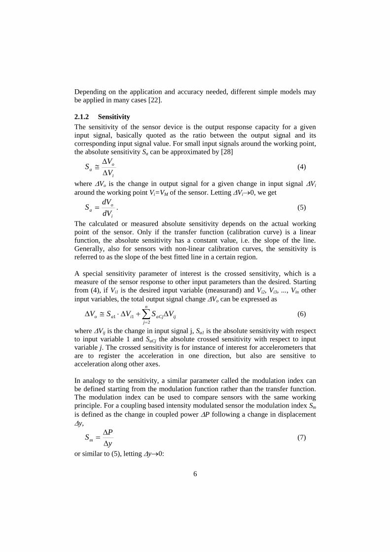
Depending on the application and accuracy needed, different simple models may
be applied in many cases [22].
2.1.2 Sensitivity
The sensitivity of the sensor device is the output response capacity for a given
input signal, basically quoted as the ratio between the output signal and its
corresponding input signal value. For small input signals around the working point,
the absolute sensitivity Sa can be approximated by [28]
i
o
aV
VS
(4)
where Vo is the change in output signal for a given change in input signal Vi
around the working point Vi=VM of the sensor. Letting Vi0, we get
i
o
adV
dVS . (5)
The calculated or measured absolute sensitivity depends on the actual working
point of the sensor. Only if the transfer function (calibration curve) is a linear
function, the absolute sensitivity has a constant value, i.e. the slope of the line.
Generally, also for sensors with non-linear calibration curves, the sensitivity is
referred to as the slope of the best fitted line in a certain region.
A special sensitivity parameter of interest is the crossed sensitivity, which is a
measure of the sensor response to other input parameters than the desired. Starting
from (4), if Vi1 is the desired input variable (measurand) and Vi2, Vi3, ..., Vin other
input variables, the total output signal change Vo can be expressed as
n
j
ijaCjiao VSVSV2
11 (6)
where Vij is the change in input signal j, Sa1 is the absolute sensitivity with respect
to input variable 1 and SaCj the absolute crossed sensitivity with respect to input
variable j. The crossed sensitivity is for instance of interest for accelerometers that
are to register the acceleration in one direction, but also are sensitive to
acceleration along other axes.
In analogy to the sensitivity, a similar parameter called the modulation index can
be defined starting from the modulation function rather than the transfer function.
The modulation index can be used to compare sensors with the same working
principle. For a coupling based intensity modulated sensor the modulation index Sm
is defined as the change in coupled power P following a change in displacement
y,
y
PSm
(7)
or similar to (5), letting y0:

7
dy
dPSm . (8)
2.1.3 Measurement Range and Dynamic Range
The measurement range is the range of input parameter values that can be
measured with a particular quality by the sensor device:
],[ max,min, ii VVMR (9)
For a coupling based intensity modulated sensor the measurement range may be
defined from a set of displacement values that are within a certain range. The
difference between the upper and lower values in the measurement range, Vi,max-
Vi,min, is called the span.
A related parameter is the dynamic range, which is another measure of the span
between the maximum and minimum input values. The dynamic range is often
expressed in dB with respect to the corresponding output parameter values
Vo(Vi,max) and Vo(Vi,min):
)(
)(log20
min,
max,
io
io
VV
VVDR (10)
2.1.4 Linearity
The linearity is a measure of the maximum deviation in output signal value from an
ideal, linear transfer function. The absolute linearity is defined as
isabs ddL ,max , (11)
where ds and di are the superior and inferior deviations from the ideal line. Further,
the relative linearity (in %) can be defined as
100
)(
,max
max,max,
io
is
relVV
ddL , (12)
where Vo,max(Vi,max) is the superior output signal value taken at the upper value of
the measurement range Vi=Vi,max.
In cases where the ideal transfer function is not linear, the linearity is more
generally referred to as conformity.
8
2.2 SENSOR INTERROGATION
One of the main advantages with intensity modulated sensors is that the
interrogation equipment is basically simple and inexpensive. Most coupling based
intensity modulated sensors can be interrogated using an LED and a p-i-n photo
diode together with various amounts of electronics. A major concern is though the
need for intensity referencing due to unwanted loss changes. Temperature effects,
ageing of components and fibre bend losses are some causes of error. This means
that the sensor system needs to adjust for variations in for instance output power
from the light source or for loss changes in the optical link. Furthermore different
system architectures may be used in order to be able to interrogate several sensors
from a single system.
2.2.1 Referencing Techniques
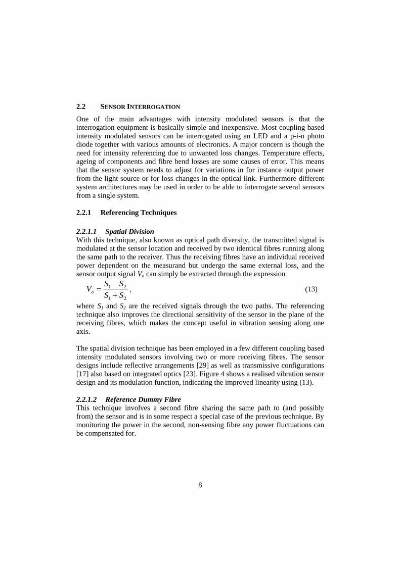
2.2.1.1 Spatial Division
With this technique, also known as optical path diversity, the transmitted signal is
modulated at the sensor location and received by two identical fibres running along
the same path to the receiver. Thus the receiving fibres have an individual received
power dependent on the measurand but undergo the same external loss, and the
sensor output signal Vo can simply be extracted through the expression
21
21
SS
SSVo
, (13)
where S1 and S2 are the received signals through the two paths. The referencing
technique also improves the directional sensitivity of the sensor in the plane of the
receiving fibres, which makes the concept useful in vibration sensing along one
axis.
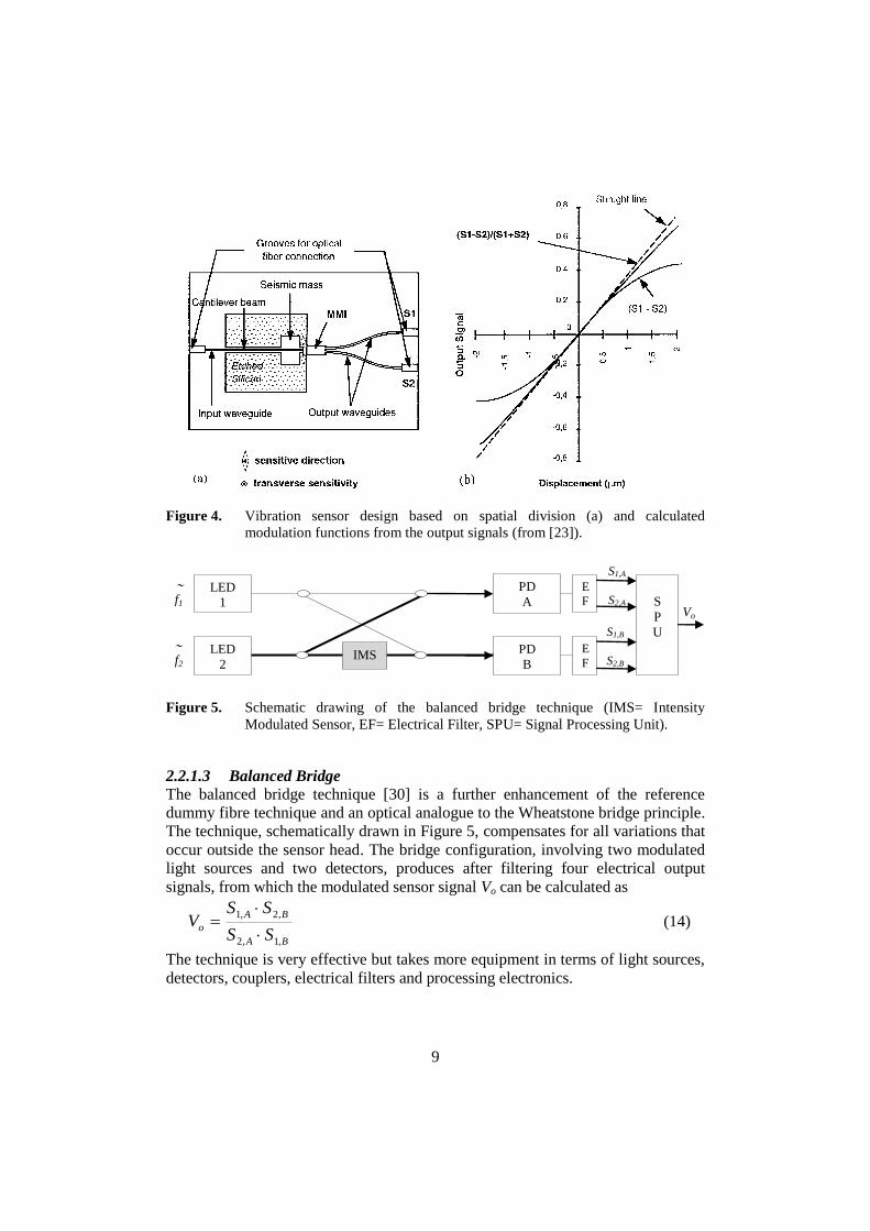
The spatial division technique has been employed in a few different coupling based
intensity modulated sensors involving two or more receiving fibres. The sensor
designs include reflective arrangements [29] as well as transmissive configurations
[17] also based on integrated optics [23]. Figure 4 shows a realised vibration sensor
design and its modulation function, indicating the improved linearity using (13).
2.2.1.2 Reference Dummy Fibre
This technique involves a second fibre sharing the same path to (and possibly
from) the sensor and is in some respect a special case of the previous technique. By
monitoring the power in the second, non-sensing fibre any power fluctuations can
be compensated for.
9
Figure 4. Vibration sensor design based on spatial division (a) and calculated
modulation functions from the output signals (from [23]).
Figure 5. Schematic drawing of the balanced bridge technique (IMS= Intensity
Modulated Sensor, EF= Electrical Filter, SPU= Signal Processing Unit).
2.2.1.3 Balanced Bridge
The balanced bridge technique [30] is a further enhancement of the reference
dummy fibre technique and an optical analogue to the Wheatstone bridge principle.
The technique, schematically drawn in Figure 5, compensates for all variations that
occur outside the sensor head. The bridge configuration, involving two modulated
light sources and two detectors, produces after filtering four electrical output
signals, from which the modulated sensor signal Vo can be calculated as
BA
BA
oSS
SSV
,1,2
,2,1
(14)
The technique is very effective but takes more equipment in terms of light sources,
detectors, couplers, electrical filters and processing electronics.
LED
1
LED
2
PD
B
PD
A
IMS
S
P
U
E
F
E
F
S1,B
S2,B
f1
f2
S1,A
S2,A
Vo

10
Figure 6. Principle layout for a wavelength referencing system (BLS= Broadband Light
Source, IMS= Intensity Modulated Sensor).
2.2.1.4 Wavelength Referencing
Rather than using two fibre channels, this technique uses two wavelengths for
sensing and referencing purposes respectively. This means that a single fibre can
be used to and from the sensor. The technique builds upon three assumptions: (1)
the system loss is significantly independent of the wavelengths used, (2) the output
power ratio between the wavelength sources is constant over time and (3) the
relative sensitivity of the detection system at the two wavelengths remains
constant. Any contradictions to these can be eliminated by the right choice of
wavelengths and components [28]. A typical system architecture is shown in
Figure 6, using a broadband light source and WDM filters for the spectral
referencing. Even better performance is achieved by using more than two
wavelengths, also known as chromatic monitoring. The wavelength referencing
technique is also used in fluorescence, absorption and black body radiation sensors
where sensing is based on measurement of intensity ratios between wavelengths.
2.2.1.5 Frequency Division (AC/DC Referencing)
This technique, more specifically referred to as AC/DC referencing, is performed
in the electrical domain and is based on measuring the ratio between the AC
amplitude and the DC level of the output signal in sensing applications where the
measurand has an AC behaviour. The inverse procedure can also be applied, using
an AC-modulated light source, when the measurand shows a DC output.
The AC/DC referencing technique is very simple to implement since it only
requires additional electronics. Typical applications include vibration sensors and
AC current sensors [31].
2.2.2 Multiplexing Techniques
Optical fibre sensor networks are either passive, where the active equipment such
as light sources and detectors are situated at one location, or active with optical
amplifiers placed within the network. Active networks are used to compensate for
distribution losses in passive networks by equalising the power between channels
and to extend the distance range.
BLS
PD 1 W
D
M PD 2
IMS

11
Figure 7. General, non-multiplexed fibre sensor network consisting of N sensors, each
with one light source and one detector (LS= light source, PD= photo detector,
DME= demodulation electronics).
Principally all passive sensor networks can be discussed starting from Figure 7. In
this basic network each sensor has its own light source, detector, lead-in fibre, lead-
out fibre and demodulation electronics. The driving force behind multiplexing is to
cut the system cost per sensor by letting a number of sensors share system
components. Besides cost, important parameters to consider in the network design
are noise, bandwidth, power budget and flexibility [32, 33]. When the primary
choice of sensor technology has been made, the next step is to choose a suitable
network topology and multiplexing technique. Some basic network topologies for
both transmission kind and reflective types of sensors are shown in Figure 8, and in
the following subsections a few passive network multiplexing techniques
applicable to intensity modulated sensors are briefly presented.
2.2.2.1 Spatial Division Multiplexing (SDM)
This technique, sometimes also denoted fibre multiplexing, is based on the idea
that several sensors share the same light source. This is accomplished by using a
star coupler, a splitter or a switch to direct the light from the source fibre to the
sensors in the network. A further step is detector sharing, which is realised in the
same way. The network topologies shown in Figure 8 are all of this kind. A special
case is the use of optical time domain reflectometry (OTDR), which lets the input
fibre also work as return fibre. The OTDR technique has its most common
application in the fibre-optic communications industry, where it is used to measure
attenuation, point loss and also other fibre parameters all from fibre manufacturing
to field. The technique is based on measurement of the back-scattered power from
laser pulses sent in to the fibre, where the time of flight gives a time and distance
resolved measurement. In Figure 9 a typical OTDR trace is shown. The reflective
type topologies (a), (b) and (c) of Figure 8 are all examples of topologies
applicable to an OTDR. In these examples each sensor should be located at a
unique distance from the OTDR in order to be identified and read out from the
OTDR trace.
LS S1 PD DME V1
LS S2 PD DME
LS SN PD DME
V2
VN

12
Figure 8. Point sensor network topologies: reflective type (a) linear, (b) star, (c) tree,
and transmissive type (d) ring, (e) star, (f) ladder (LS= Light source, PD=
Photo detector, S= Sensor).
Figure 9. An OTDR trace showing different typical events.
(e)
(d)
(f)
LS
PD
S S
S
S
LS
PD
D
S S S S
LS
PD
S S S S
(a)
(c)
(b)
LS
PD
S
S
S
S
LS
PD
S S S
S
LS
PD
S
S
S
S
S
S S

13
2.2.2.2 Time Division Multiplexing (TDM)
Time division multiplexing in its simplest form is performed by operating a switch
in a star network on a time sharing basis, see Figure 8(b) and Figure 8(e). One
problem with that approach is that only a limited operating time is available for
each sensor during the switching sequence.
A more attractive approach is to use the OTDR technique in the reflective star
network of Figure 8(b), and connecting the sensors with different lengths of fibre.
Alternative OTDR-based solutions are reflective linear, Figure 8(a), or
transmissive ladder networks, Figure 8(f). The returning (or transmitted) pulses
will then have individual delays associated with different sensors. Furthermore, for
absorption (loss) type sensors, another way is to connect the sensors in series in a
transmissive linear network, also leading to a sensor-specific time delay. The latter
concept is however limiting the number of sensors if a particular resolution is
required, and there is also a risk for signal loss of all sensors if the first sensor fails.
Due to its capability of measuring reflection and absorption events at any location
along a fibre, the OTDR technique is well suited for distributed sensing of a
number of parameters along an installed cable length [7-10].
An alternative TDM method is Optical Frequency Domain Reflectometry (OFDR),
where a chirped frequency modulation is applied to the light source. The returning
light from the sensors is mixed with the input light at the detector, where the time
delay for each sensor corresponds to a beat frequency in the spectrum. The
intensity for each beat frequency is then the readout from the intensity modulated
sensor. Although the demodulation of the sensors take place in the frequency
domain OFDR could be considered as a TDM technique since each sensor is
associated with an individual time delay.
2.2.2.3 Frequency Division Multiplexing (FDM)
Frequency division multiplexing is realised by addressing each sensor with its own
frequency channel, within which the sensor signal amplitude (or frequency or
phase in the case of other sensing techniques) can be modulated by the measurand.
Two groups within this technique can be identified: subcarrier FDM, which uses a
light source (typically an LED) modulated at a number of frequencies, and
frequency-encoded sensor multiplexing, where each sensor respond to the input
signal with a unique resonance frequency.
2.2.2.4 Wavelength Division Multiplexing (WDM)
Wavelength division multiplexing can be considered a special case of the FDM
technique, the main difference being that the WDM technique uses the optical
spectrum. The WDM technique can be adopted for both reflective and transmission
type sensors, using either a set of narrow-band light sources or a broadband source
together with filters or dispersive components. A few concepts involving intensity
modulated sensors are shown in Figure 10.

14
(a)
(c) (b)
MLS SN
DE
MU
X
S2
1
2
N
I(1,2,…,N)
S1
I(1,2,…,N)
I(1)
I(N)
I(2)
PDA
1
2
N
DE
MU
X
BLS
SN
MU
X
S2
S1 I(1)
I(N)
I(2)
PD
A
1
2
N
DEMUX
BLS
S1 S2
1 2 N
DE
MU
X
PDA
1
2
N
F1 FN F2
SN
Figure 10. WDM sensor networks for intensity modulated sensors; (a) transmissive star
network with multisource module, (b) transmissive ladder network with
broadband source, (c) reflective star network with broadband source (MLS=
Multiple light source, BLS= Broadband light source, PDA= Photo detector
array, F= Optical filter).
2.3 MODULATION FUNCTION MEASUREMENTS AND MODELLING
As pointed out earlier, the modulation function plays an important role in the
design and modelling of a coupling based intensity modulated sensor. Much of the
theory behind can be taken from the splice loss theory evolved in the late 70’s and
early 80’s [24]. Later models, specifically developed for coupling based sensors,
are also available [26, 27]. In the case of multimode fibre based sensors the
measurement of the modulation function is of great importance, since there are no
precise theoretical models at hand.
The work in this thesis is concentrated on the design of transmissive coupling
based intensity modulated sensors, see Figure 2(a), using the lateral movement of
the transmitting fibre for modulation. Such a device can for instance be used for
vibration sensing. An interesting feature for this application is the sensitivity of the
sensor, which is determined by the slope of the modulation curve, also denoted the
modulation index. The design process must also take parameters such as
measurement range and coupled power into account.
In order to increase the sensitivity of the sensor, a multiple pass configuration has
been proposed [34]. In this case the light is coupled back from the first receiving
fibre to a second, parallel transmitting fibre, further to a second receiving fibre and
so on until a number of passes over the gap has been completed. The idea is that
the multiple passes should increase the sensitivity by simply introducing a higher
loss in coupled power for a certain lateral transmitting fibre displacement. The
possibility of realising this has been analysed experimentally and theoretically
within the work behind this thesis, and has been presented in [35].

15
2.3.1 Measurements
For precise and efficient measurements of the modulation function a modulated
light source and a lock-in amplifier should be used together with a computer
controlled micropositioner [24, 27]. Also the modal distribution of the light source
should be considered and controlled in multimode fibre measurements [24]. In the
case under scope in this thesis, we are not looking for exact data for the fibres but
for data to compare the modulation function between different fibre configurations
and the effect of using multiple passes. A simplified setup, shown in Figure 11, has
therefore been used.
Unless unwanted bending effects are present, the modulation function is
independent of the wavelength, which has been shown experimentally [24].
Measurement at one single wavelength is therefore sufficient for modulation
function comparison between different fibre types. The light source chosen for the
measurements was an LED operating in continuous mode at 1300 nm.
Figure 11. Modulation function measurement setup.
2.3.1.1 Single pass configuration
Measurements of the modulation function were made with the setup shown in
Figure 11. The fibres under test, each about 5 m long, were stripped in one end and
cleaved just about a mm from the coating. Pigtails were fusion spliced to the
opposite ends of the test fibres in order to establish stable connection to the light
source and the detector. Using a bare fibre connection to the detector, the output
power Pout from the transmitting fibre end was measured. The cleaved fibre ends
were then inserted into clamping holders with only the bare fibre protruding from
the holders.
The transmitting fibre holder was fixed onto a xyz-translator stage, and the
receiving fibre holder was mounted on a fixed stage. Before setting the fibre pair
into the desired axial (longitudinal) offset, the fibre ends were put into physical
contact and then set at 10 µm axial offset. Further, the vertical (y-) and horizontal
(x-) position was adjusted for maximum transmitted power, and the ends were
brought into physical contact again. The transmitted power at zero axial offset was
1300 nm LED
Power meter
Transmitting fibre (5 m)
Receiving fibre (5 m)
xyz- stage
Fixed stage
Detector
16
recorded, and the fibres were put into the desired axial offset position, where the
transmitted power at zero vertical offset was recorded. Measurements of the
transmitted power P(y) for vertical offsets y ranging from –50 µm to +50 µm were
recorded at 1-2 µm steps.
For comparison between different fibre types, the measured transmitted power P(y)
at the vertical offset y was normalized to the output power Pout of the transmitting
fibre, defining the transmission ratio T(y) as
outP
yPyT
)()( (15)
The maximum value of T(y) is denoted T0, which is the transmission ratio at zero
offset.
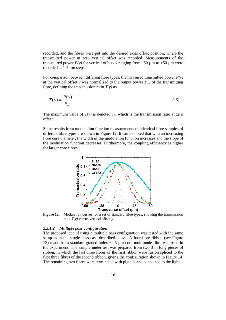
Some results from modulation function measurements on identical fibre samples of
different fibre types are shown in Figure 12. It can be noted that with an increasing
fibre core diameter, the width of the modulation function increases and the slope of
the modulation function decreases. Furthermore, the coupling efficiency is higher
for larger core fibres.
Figure 12. Modulation curves for a set of standard fibre types, showing the transmission
ratio T(y) versus vertical offset y.
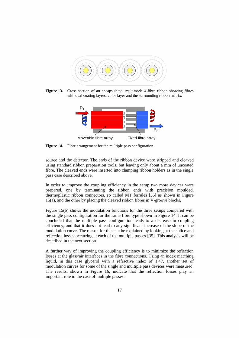
2.3.1.2 Multiple pass configuration
The proposed idea of using a multiple pass configuration was tested with the same
setup as in the single pass case described above. A four-fibre ribbon (see Figure
13) made from standard graded-index 62.5 µm core multimode fibre was used in
the experiment. The sample under test was prepared from two 3 m long pieces of
ribbon, in which the last three fibres of the first ribbon were fusion spliced to the
first three fibres of the second ribbon, giving the configuration shown in Figure 14.
The remaining two fibres were terminated with pigtails and connected to the light
17
Figure 13. Cross section of an encapsulated, multimode 4-fibre ribbon showing fibres
with dual coating layers, color layer and the surrounding ribbon matrix.
PR
PT
Moveable fibre array Fixed fibre array
Figure 14. Fibre arrangement for the multiple pass configuration.
source and the detector. The ends of the ribbon device were stripped and cleaved
using standard ribbon preparation tools, but leaving only about a mm of uncoated
fibre. The cleaved ends were inserted into clamping ribbon holders as in the single
pass case described above.
In order to improve the coupling efficiency in the setup two more devices were
prepared, one by terminating the ribbon ends with precision moulded,
thermoplastic ribbon connectors, so called MT ferrules [36] as shown in Figure
15(a), and the other by placing the cleaved ribbon fibres in V-groove blocks.
Figure 15(b) shows the modulation functions for the three setups compared with
the single pass configuration for the same fibre type shown in Figure 14. It can be
concluded that the multiple pass configuration leads to a decrease in coupling
efficiency, and that it does not lead to any significant increase of the slope of the
modulation curve. The reason for this can be explained by looking at the splice and
reflection losses occurring at each of the multiple passes [35]. This analysis will be
described in the next section.
A further way of improving the coupling efficiency is to minimize the reflection
losses at the glass/air interfaces in the fibre connections. Using an index matching
liquid, in this case glycerol with a refractive index of 1.47, another set of
modulation curves for some of the single and multiple pass devices were measured.
The results, shown in Figure 16, indicate that the reflection losses play an
important role in the case of multiple passes.

18
Figure 15. (a) Endface of MT ferrule terminating a 12-fibre ribbon, (b) Modulation
curves for multiple pass configurations, using different alignment techniques
(R4, V4, MT4), compared to a single fibre pair.
Figure 16. Modulation curves for a single (1x) and multiple (MT4) pass configurations,
with and without index matching liquid.
2.3.2 Modelling
For the purpose of having a simple model describing the general behaviour of the
modulation function, a Gaussian expression is used for the received optical power
P versus the vertical offset y (or more general the radial offset r): 2
0)(
w
y
ePyP (16)
where P0 is the received power at zero vertical offset and w is the characteristic
radius of the power distribution, not to be confused with the mode field radius of
the electrical field distribution. Alternatively, w can be expressed in terms of the
parameter =w-2
. Using this expression and (15) gives the following expression for
the transmission ratio:
19
2
0)( yeTyT (17)
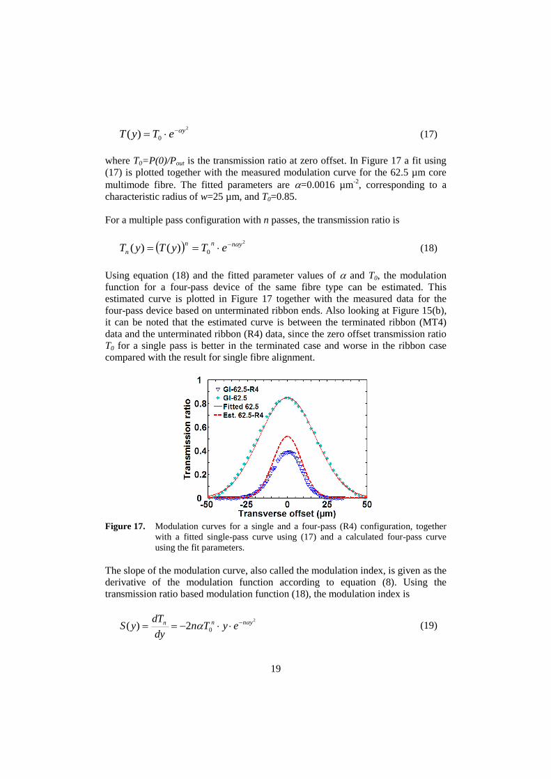
where T0=P(0)/Pout is the transmission ratio at zero offset. In Figure 17 a fit using
(17) is plotted together with the measured modulation curve for the 62.5 µm core
multimode fibre. The fitted parameters are =0.0016 µm-2
, corresponding to a
characteristic radius of w=25 µm, and T0=0.85.
For a multiple pass configuration with n passes, the transmission ratio is
2
0)()( ynnn
n eTyTyT (18)
Using equation (18) and the fitted parameter values of and T0, the modulation
function for a four-pass device of the same fibre type can be estimated. This
estimated curve is plotted in Figure 17 together with the measured data for the
four-pass device based on unterminated ribbon ends. Also looking at Figure 15(b),
it can be noted that the estimated curve is between the terminated ribbon (MT4)
data and the unterminated ribbon (R4) data, since the zero offset transmission ratio
T0 for a single pass is better in the terminated case and worse in the ribbon case
compared with the result for single fibre alignment.
Figure 17. Modulation curves for a single and a four-pass (R4) configuration, together
with a fitted single-pass curve using (17) and a calculated four-pass curve
using the fit parameters.
The slope of the modulation curve, also called the modulation index, is given as the
derivative of the modulation function according to equation (8). Using the
transmission ratio based modulation function (18), the modulation index is
2
02)( ynnn eyTndy
dTyS (19)

20
The maximum modulation index, i.e. the maximum absolute value of the slope of
the modulation curve, occurs for y=1/(2n)=w/(2n). Given a fixed value for
, and with 0T01 and n1, the maximum modulation index Smax is a function of n
and T0:
e
n
w
T
e
nTTnS
n
n 22),( 0
00max
(20)
With the fitted value of =0.0016 µm-2
, the maximum modulation index Smax can
be plotted versus T0 for different number of passes n. This is done in Figure 18,
which shows that in order to get a benefit in modulation index with a multiple pass
configuration, T0 needs to be high. For an increasing number of passes, the demand
on T0 gets even higher. A four-pass device requires T0>0.78 to reach a higher Smax
than a single-pass device.
Figure 18. The maximum modulation index for a 62.5 µm fibre device as a function of
the zero offset transmission ratio for different number of passes.
The transmission ratio T0 at zero offset should account for all other factors than the
vertical offset having an impact on the coupled power. The main factors are the
Fresnel reflection occurring at glass/air interface and the horizontal and
longitudinal offsets that remain constant after the setup. Also intrinsic factors such
as differences in fibre geometry between the coupled fibres should be accounted
for, but can be ignored if identical fibres are used. With this background we can
write T0 as
aF TTT 0 (21)
with TF being the Fresnel reflection related part and Ta the alignment dependent
part, ignoring contribution from intrinsic factors. TF can be calculated as the total
transmission coefficient involved in a single pass, i.e. involving two glass/air
interfaces, as

21
22
2 1)1(
airglass
airglass
airglassFnn
nnRT (22)
where Rglass-air is the reflection coefficient for a glass/air interface and nglass and nair
are the refractive indices for glass and air respectively. Using nglass=1.5 and nair=1.0
we get TF=0.962=0.92 for a single fibre pass. With the fitted T0=0.85 to the 62.5
µm core fibre, this makes the alignment dependent part Ta=T0/Ta=0.85/0.92=0.92
for a single pass.
2.4 INDUSTRIAL SENSING APPLICATIONS
Over the years, a number of industrial applications and different designs of fibre-
optic sensors based on intensity modulation using coupling have been suggested.
Though other technologies have advanced and developed there has still been
interest for this kind of sensors, much due to the simplicity and low cost that they
intend to offer.
2.4.1 Applications in Position and Vibration Sensing
An ideal accelerometer includes a concentrated mass that is connected to the sensor
housing via an elastic element. Fibre-optic or integrated optics accelerometers can
be realized by using a shutter configuration [22] or a waveguide cantilever design
[23]. In the latter case this can be accomplished using integrated optics or letting a
fibre act as the cantilever. In the case of semiconductor materials, most often
silicon, a seismic mass can be integrated in the cantilever or shutter tip using
etching or micro-machining methods. When using a fibre cantilever, a ball lens can
be formed at the end of the fibre by means of fusion splicing [21]. These
modifications however involve extra processing steps. It has been shown though
that in a frequency range sufficiently low compared with the resonance frequency,
a cantilever without any seismic mass behaves as an ideal accelerometer with a
very small error [37].
An industrially applied fibre-optic accelerometer based on a fibre cantilever is
shown in Figure 19. The accelerometer was designed for the monitoring of the
bearings in a hydroelectric generator [38] and successfully installed and operated
[39]. The sensor uses the spatial division referencing technique, thereby assuring
stable operation and low directional cross sensitivity of the sensor.
Figure 19. A fibre-optic accelerometer using a fibre cantilever (from [39]): sensor
principle (left) and photo of sensor head (right).

22
2.4.2 Temperature Measurement Applications
The coupling based intensity modulation technique can be applied not only to
position and displacement sensing, but to any property that can be put into relation
with displacement. Temperature sensing is such an example, in which the
displacement can be actuated by temperature by means of a bimetal strip. The
bimetal is a two-layer strip consisting of an alloy with high thermal expansion on
top of a layer with negligible thermal expansion. Bimetals have proven to be
reliable in their conventional use in thermostats, but they have also had some
applications in fibre-optic sensing. In [40] a U-shaped bimetal element is utilized
for the movement of the transmission fibre. The sensor solution is based on
multimode fibre with 400 µm core diameter and includes a spatial division
referencing technique. Another solution is presented in [41], where a reflective
arrangement is used involving chromatic modulation, based on optical filters,
rather than intensity modulation. A reflective arrangement is also used in [42],
where the displacement of a grating, moved by a bimetal strip and a lever
framework, is measured.
A bimetal-based temperature sensor for the purpose of monitoring the cooking
process of wood chips in pulp production has been developed and installed [43].
The cooking process is very crucial for the quality of the pulp, and therefore
continuous process monitoring at distributed points is needed. Figure 20(a) shows
the cooking liquor flows and circulation pipes of the actual digester. The sensor,
shown in Figure 20(b), is intended to be surface mounted and placed on a pipe as
shown in Figure 21, which means that it measures the outer temperature of the pipe
wall rather than the temperature of the liquid flowing through the pipe. This is an
important feature due to the hazardous chemicals used in the cooking process,
which involves temperatures of typically 140-150 °C. The temperature monitoring
is to be performed at six distributed points at each of three circulation levels of the
digester, see Figure 20(a).
Y
Receiving connector (adjustable)
Transmitting connector (adjustable) on bimetal strip (hidden)
PTFE tube
X
Figure 20. (a) Cooking liquor flows in digester and conventional temperature monitoring
points. (b) Fibre-optic temperature sensor prototype for cooking process
monitoring.
(b) (a)

23
Figure 21. Temperature sensor installation on cooking liquor circulation pipe, cross
section (left) and front view (right)
2.4.2.1 Modelling of a Fibre Coupling Actuated by a Bimetal Strip
The temperature dependent deflection of a bimetal strip clamped at one end is
given by
t
LTTd
2
0
0 )( (23)
where d is the specific deflection, T the temperature, L0 the free strip length at
room temperature T0 and t the strip thickness. For a fibre sensor configuration
according to Figure 22, L0 equals the fibre position on the free bimetal strip and
corresponds to the vertical fibre offset y according to equation (16). In the linear
temperature region of the bimetal strip, the deflection can be counted from any
reference temperature T0, which means that the reference temperature could be
chosen when the moveable fibre has a zero offset to the fixed fibre. The coupled
power P as a function of temperature T can thus be written
2
0 )(
0)(TTk
ePTP
(24)
where P0 is the coupled power at temperature T0, i.e. at zero offset (deflection),and
the design factor k is given by
2
2
0
t
L
wk d
(25)
where w is the characteristic radius of the modulation function. From (24) the
temperature dependent loss A of the sensor, quoted in decibels (dB), can be derived
as
2
0
0 )()(
)(log10)( TTK
TP
TPTA (26)
Pipe wall
Sensor mount
Sensor
Cooking liquor
Insulation
Hood
Splice closure

24
where the design constant K is given by
et
L
wK d log10
22
0
(27)
Using formulas (23), (26) and (27) a temperature sensor for any temperature range
in the linear region of the bimetal can be designed. The sensitivity of such a sensor
can be adjusted by choosing a suitable bimetal (parameters d and t) and by
adjusting the free strip length L0. The variable sensitivity feature is also pointed out
in [20]. For linearity reasons the measurement range should correspond to fibre
displacements on the nearly linear part of the modulation curve (see Figure 23). T0
should therefore be chosen to be a bit lower than the minimum temperature Tmin to
be measured, or a bit larger than the maximum temperature Tmax if using the left
slope of the curve in Figure 23. Depending on the power budget for the sensor
system, Tmax (or Tmin in the latter case) should correspond to a deflection m
between the minimum value min and maximum value max in the linear deflection
range.
Figure 22. Temperature sensor operation principle.
Figure 23. Measured and fitted modulation curves for a connection between two graded-
index 62.5 µm diameter core multimode fibres, showing the bimetal
deflection range for sensor design. The characteristic radius w=25 µm.
t
L0
Fixed fibre
=0 (T=T0) min max

25
From Figure 23 it can be concluded that the maximum sensor loss available in the
linear region of the modulation curve is
)(log10
max
0
maxP
PA (28)
which gives Amax= 10log(0.85/0.18) dB = 6.7 dB for the modulation curve shown
in Figure 23, corresponding to max=30 µm. Analogue to this, the loss at the
minimum temperature is Amin=10log(0.85/0.80) dB = 0.32 dB corresponding to
min=5 µm. The temperature span Tmax-T0 (or Tmin-T0 for the left slope) should
correspond to a loss up to Amax depending on the power available in the system. In
the pulp industry application under scope the measurement range of interest, [Tmin,
Tmax], is [130, 170] °C.
Using (23), the deflection range is given by
)( minmax
2
0
min TTt
Ld
m
(29)
where m is the desired maximum deflection and Tmax and Tmin are the maximum
and minimum temperatures of the measurement range, corresponding to the desired
deflection range. From (29) the fibre position L0 can be calculated, and using this
value together with =min and T=Tmin, equation (23) gives the zero deflection
temperature T0 for the right slope of the modulation curve. For the left slope of the
modulation curve, T=Tmax and =-min should be chosen instead. The minimum loss
Amin and the maximum loss Amax in the temperature range can finally be calculated
using (26) and (27). The difference Amax-Amin is a measure of the dynamic range of
the sensor.
In Table 1 some calculated sensor design data are given for three different bimetal
strips [44] using the above design principles and the right slope of the modulation
curve. The sensor parameters are calculated for the deflection ranges = 10 µm,
16 µm and 25 µm respectively in order to illustrate the difference in allowable
dynamic range. A proper choice of bimetal can be made depending on the choice
of free strip length for a certain dynamic range. Another parameter to be considered
is the thermal conductivity, which should be high in order to give a fast response
for the sensor. The bimetal types listed in Table 1 have thermal conductivities of 6
Wm-1°C
-1 (type 230), 13 Wm
-1°C
-1 (type 115) and 44 Wm
-1°C
-1 (type 60)
respectively.
The sensitivity of the sensor in terms of the loss change in dB per temperature
degree is given by the derivative of (26):
)(2)( 0TTKdT
dATS (30)

26
with K given by (27). The sensitivity is linear function of temperature and is
largely dependent on the K value. The sensitivity for the type 230 bimetal sensor
designs in Table I is plotted in Figure 24. The minimum sensitivity ranges from
0.02 dB/°C to 0.06 dB/°C between the design examples, and the maximum
sensitivity from 0.05 dB/°C to 0.37 dB/°C. For a certain desired temperature
resolution in the measurement, the sensitivity of the sensor needs to be considered
in the design depending on the resolution of the power monitoring equipment used
for interrogation.
Table I. Bimetal data and calculated sensor design parameters for min= 5 µm, Tmin=
130 °C and Tmax= 170 °C using a fibre coupling with a characteristic radius of
w= 25 µm. Italic number shows example of left slope data using =-min= -5
µm and T=Tmax=170 °C in (23).
Type
d
(10-6
K-1
)
t
(mm)
(µm)
L0
(mm)
T0
(°C)
K
(10-3
dB
K-2
)
A(Tmin)
(dB)
A(Tmax)
(dB)
230 22.7 1.3 10 3.8 110 0.43 0.17 1.56
16 4.8 118 1.11 0.17 3.06
25 6.0 122 2.71 0.17 6.25
30 6.6 177 3.91 8.51 0.17
115 11.7 0.8 10 4.1 110 0.43 0.17 1.56
16 5.2 118 1.11 0.17 3.06
25 6.5 122 2.71 0.17 6.25
60 6.0 1.0 10 6.5 110 0.43 0.17 1.56
16 8.2 118 1.11 0.17 3.1
25 10.2 122 2.71 0.17 6.3
Figure 24. Sensitivity as a function of temperature for the sensor designs based on type
230 bimetal listed in Table I.
=25 µm
=16 µm
=10 µm
=30 µm
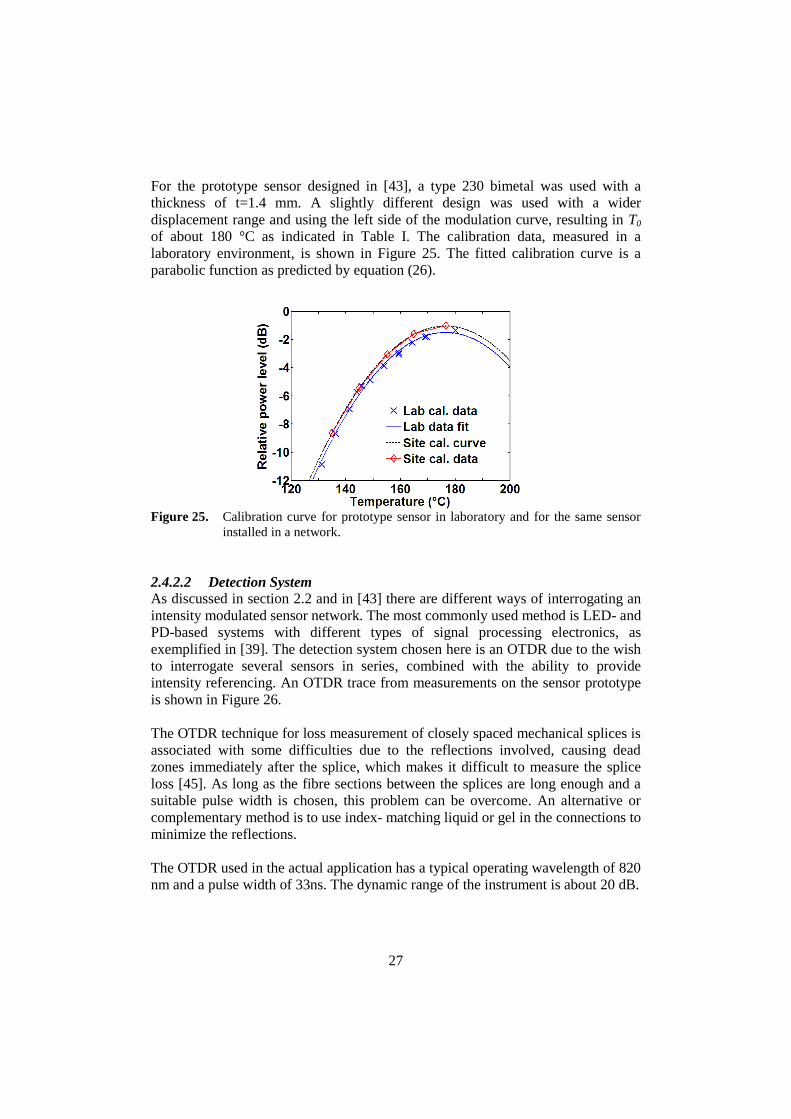
27
For the prototype sensor designed in [43], a type 230 bimetal was used with a
thickness of t=1.4 mm. A slightly different design was used with a wider
displacement range and using the left side of the modulation curve, resulting in T0
of about 180 °C as indicated in Table I. The calibration data, measured in a
laboratory environment, is shown in Figure 25. The fitted calibration curve is a
parabolic function as predicted by equation (26).
Figure 25. Calibration curve for prototype sensor in laboratory and for the same sensor
installed in a network.
2.4.2.2 Detection System
As discussed in section 2.2 and in [43] there are different ways of interrogating an
intensity modulated sensor network. The most commonly used method is LED- and
PD-based systems with different types of signal processing electronics, as
exemplified in [39]. The detection system chosen here is an OTDR due to the wish
to interrogate several sensors in series, combined with the ability to provide
intensity referencing. An OTDR trace from measurements on the sensor prototype
is shown in Figure 26.
The OTDR technique for loss measurement of closely spaced mechanical splices is
associated with some difficulties due to the reflections involved, causing dead
zones immediately after the splice, which makes it difficult to measure the splice
loss [45]. As long as the fibre sections between the splices are long enough and a
suitable pulse width is chosen, this problem can be overcome. An alternative or
complementary method is to use index- matching liquid or gel in the connections to
minimize the reflections.
The OTDR used in the actual application has a typical operating wavelength of 820
nm and a pulse width of 33ns. The dynamic range of the instrument is about 20 dB.

28
-10
-8
-6
-4
-2
0
2
0 50 100 150 200 250
Rela
tive P
ow
er
Level
(dB
)
Position (m)
A B
S
Figure 26. OTDR trace from measurements on the installed sensor prototype. The sensor
(S) is preceeded and followed by about 115 m of fibre.
2.4.2.3 Sensor Network
The sensor network built is a combined spatial and time division multiplexed
network as shown in Figure 27. The six sensor positions per level are associated
with six channels of the switch (spatial division), and the sensors on the same
position at each level are put in series on the actual channel (time division).
Instead of using conventional cabling, fibre units (EPFU:s) are blown into micro-
ducts installed between the control room and the sensor locations. The blown fibre
technique is since many years established in fibre-to-the-home (FTTH)
installations due to the cost-efficiency and flexibility it offers [46, 47]. The same
advantages are of interest in the sensor network in this study: the flexibility in the
installation allows for micro-ducts to be installed at one time, and fibre units blown
into the network as sensors are installed. This leads to efficient and less costly
sensor system installations since the time for specialized installation of sensors and
connecting fibres can be shortened [48].
The complete sensor network layout is shown in Figure 28. Multiducts with seven
tubes are installed over the distance of about 110 metres between the control room
and the digester. From the joint closure at the end the connections are branched out
to the individual sensor locations using single microducts. Each of the six sensors
S11, S21, ..., S61 on the first circulation level is connected with 2-fibre EPFU:s to the
fibre-optic switch in the control room, thereby realising a spatial division
multiplexed network as described above. The sensor Si1 at a certain position is
connected serially to the corresponding sensors Si2 and Si3 at the two upper

29
circulation levels, utilizing a time division multiplexing scheme with the OTDR
monitoring system in the control room. The 2-fibre units and the double channel
capacity of the switch also allow for bi-directional measurements to be made. In
the prototype installation studied however only one sensor on the first circulation
level is connected.
Figure 27. Network topology for the temperature sensor system using combined spatial
and time division multiplexing.
High temperature zone
(cooking system)
Outdoor environment
Indoor environment
OTDR
Fiber - optic s witch
ODF
Joint
closure Multid uct (7x)
out door
( 15 m)
Joint
closure
Single microduct
outdoor
( 5 m)
Multiduct (7x)
indoor
(90 m)
Splice
closure
1 2
3
4 5
6
L evel 2
L evel 1
L evel 3
Control unit
and monitor
Sensor
Figure 28. Complete temperature sensor system network layout.
OTDR
S11 S12 S13
S21 S22 S23
S31 S32 S33
S41 S42 S43
S51 S52 S53
S61
S62 S63

30
2.4.2.4 Monitoring Results
The computer controlling the OTDR is also equipped with data acquisition routines
and system calibration data files. The calibration data (see Figure 25), acquired
after installation of the sensor by a simple loss offset measurement at a referenced
temperature, is used for the conversion of a measured sensor loss value to a
temperature value.
In Figure 29 the temperature over eight days measured by the fibre-optic sensor
(FOS) at position 1 at level 1 is shown together with the temperature measured by
the conventional plug-in sensor (Pt) at the common pipe of circulation level 1. The
variations in temperature data seem to agree well, bearing in mind that the
conventional sensor consequently measures an average temperature of all outflows
at level 1. The largest temperature drops in the circulation temperature data are due
to the fact that the circulation has been turned off on these occasions. The level
difference between the two curves depend on the measurement technique: the
conventional sensor measures the liquid temperature, and the fibre-optic sensor
measures the surface temperature of the pipe.
Figure 30 and Figure 31 show temperature plots over a shorter (48 hours) and
longer time (4 weeks), respectively. Again the temperature trends are equal, but
especially for the short time plot there are also signs of variations which may
indicate the fact that the fibre-optic sensor is able to measure the local temperature.
This is interesting for the intended installation of six sensors at the same circulation
level, and the possibility of localizing temperature drops by comparing the
temperature data from these sensors.
130
135
140
145
150
155
160
4-Aug
0:00
5-Aug
0:00
6-Aug
0:00
7-Aug
0:00
8-Aug
0:00
9-Aug
0:00
10-Aug
0:00
11-Aug
0:00
12-Aug
0:00
Time
Tem
pera
ture
(°C
)
Level 1, Outflow 1 (FOS)
Level 1, Circulation (Pt)
Figure 29. Temperature monitoring results during 8 days.

31
130
135
140
145
150
155
160
13-jul
00:00
13-jul
06:00
13-jul
12:00
13-jul
18:00
14-jul
00:00
14-jul
06:00
14-jul
12:00
14-jul
18:00
15-jul
00:00
Time
Te
mp
era
ture
(°C
)
Level 1, Circulation (Pt)
Level 1, Outflow 1 (FOS)
Figure 30. Temperature monitoring results during 2 days.
130
135
140
145
150
155
160
25-aug 0:00 01-sep 0:00 08-sep 0:00 15-sep 0:00 22-sep 0:00
Time
Te
mp
era
ture
(°C
)
Level 1, Sensor 1 (FOS)
Level 1, Circulation 1 (Pt)
Figure 31. Temperature monitoring results during 4 weeks.


33
3 INTENSITY MODULATED SENSORS BASED ON COUPLING
BETWEEN A SINGLE FIBRE AND A MULTICORE FIBRE OR
FIBRE BUNDLE
As discussed in the previous section, the need for special alignment procedures in
the design and fabrication of coupling based intensity modulated sensors limits
their use and cost effectiveness. Micromachining and etching of precision V-
grooves is useful in some designs [22, 38], and integrated optics may also provide
relaxation of the alignment problems in some cases [23]. The alignment issue is
still, together with the need for intensity referencing, the most problematic issue
associated with this kind of sensors. Often large diameter core fibres are to be
preferred to increase the coupled power, relax the alignment demands and lower
the sensor cost [49].
If the receiving fibre is removed and the light from a single, transmitting fibre is
directly received by a position sensitive detector (PSD) or a CCD or CMOS image
sensor, a simple position sensor without any precision alignment is needed.
Working with a direct laser beam, PSDs are widely used for a variety of position
measurements in industrial applications [50], reaching down to resolutions of 1-2
µm for standard PSDs [51]. CCD and CMOS image sensors have also found a lot
of applications [52], but while the PSD has a simple readout of the position, CCD
and CMOS sensors require additional data processing to calculate the position of
the centre of the light spot. The main advantage of a PSD is the high sampling
frequency that can be achieved: 10 kHz-10 MHz depending on the size of the PSD
[51]. With a CMOS sensor, having individual circuitry for each pixel, any part of
the sensor area can be ignored in the processing, thus leading to a higher sampling
speed in the pixel region of interest. This advantage, called windowing, is not
generally available in a CCD due to its construction with intermediate charge
transfer sites, and even without this feature the speed of a CMOS sensor is much
higher than that of a CCD sensor. On the other hand the CCD sensor has a higher
dynamic range than the CMOS sensor because of less on-chip circuitry which leads
to less noise [53]. The resolution of CCD and CMOS sensors depends on the pixel
size, which can be just a few µm, and sub-pixel resolution is possible by means of
centre of gravity calculations of the light spot.
In an environment suffering from electromagnetic disturbance all electronics
including the image sensor has to be removed from the sensing area. This means
that direct illumination of the image sensor cannot be used, but rather a coupling
based approach, using a fibre bundle or a multicore fibre. The idea is to let the
optical power distribution from the transmitting fibre be spread over a number of
cores in the receiving fibre/bundle, which transfers the power distribution to the
image sensor at the other end as shown in Figure 32. Through readout of the optical
power in each individual core and knowledge about the core positions of both ends

34
Transmitting fiber(moving end)
Receiving fiber bundle(fixed)
CMOS camera chip
- -
- -
Sensing pointDetection point
Figure 32. Sensor configuration using a single transmitting fibre and a receiving fibre
bundle coupled to an image sensor.
of the receiving fibre/bundle, the position of the transmitting fibre can be
calculated from the modulation function. In this way the alignment of the
transmitting fibre to the receiving fibre is significantly relaxed, and the system is
self-calibrating.
3.1 THEORY AND MODEL
A model of the complete sensor system including software routines for calibration
and extraction has been made and implemented in a simulator. The model consists
of three main parts: the hardware description, the calibration procedure and the
extraction procedure.
3.1.1 Hardware Description
In the hardware description the physical and optical parameters of the included
components are specified and modelled. The essential hardware parameters used in
the model are listed in Table II below.
The pixel structure of the image sensor, with the pixel size (width as, area A = ap
ap) and the number of active rows n and columns m being the basic parameters,
defines the coordinate system needed for the model.
The transmitting fibre and its axial distance to the fibre bundle are specified
through the characteristic width w of the modulation function, describing the
coupled power to a core of the receiving fibre/bundle. Analogue to (16), the
coupled power in two dimensions can be described by
2
2
22
0
)()(exp),(
w
yyxxPyxP cc (31)

35
where P0 is the coupled power at zero offset and (xc,yc) the centre position of the
transmitting fibre core. An alternative expression is to use a model for the near-
field power distribution from a graded–index multimode fibre [54]:
2
2
22
0
)()(1),(
a
yyxxPyxP cc (32)
for (x-xc)2+(y-yc)
2 ≤ a
2 and P(x,y) = 0 for (x-xc)
2+(y-yc)
2 > a
2, where a is the radius
of the intensity spot and the other parameters as in (31). The modulation function
parameters are determined by fitting procedures to experimental data. Figure 33
shows measured data and fitted curves for a coupling between a 200 µm core step-
index multimode fibre with a numerical aperture of 0.22, to a standard single-mode
fibre (ITU/T G.652) with a typical core diameter of 8.3 µm and a numerical
aperture of 0.11. For the purpose of evaluating different concepts, the Gaussian
model (31) was chosen due to its simplicity.
The core geometry of the receiving fibre/bundle, for simplicity assumed to be an
array or a square matrix, is described by the number of cores 1 N or N N, the
core-to-core distance s and the core position standard deviation s. For simulation
of the appearance of the power distribution from each individual core of the
receiving fibre/bundle, the characteristic radius wo of the modulation function for
small-gap coupling between identical fibres (see section 2.3) is used.
In the simulator the transmitting fibre can be set in any offset positions, and the
hardware description algorithms calculate the resulting intensity images at the other
end of the receiving fibre/bundle.
Table II. Simulation parameters for fibre-bundle-image sensor system
Parameter Symbol
Image sensor pixel size ap
Number of active pixel rows n
Number of active columns m
Modulation function Gaussian field radius wModulation function maximum intensity P0Number of cores in receiving fibre/bundle or N N
Core to core distance in receiving fibre/bundle s
Core position standard deviation s
Core output Gaussian field radius wo

36
Figure 33. Measured and fitted modulation curves for a coupling between a 200 µm core
fibre and a standard single-mode fibre at an axial distance of 3000 µm.
3.1.2 Calibration Procedure
The calibration procedure takes care of the calibration of the geometrical
parameters of the system hardware: the core centre positions of both ends of the
receiving fibre/bundle and the transmitting fibre core centre position (xc,yc).
The centre positions of the receiving fibre/bundle cores are found by illuminating
all cores of the opposite, receiving end (R-end) and searching for local maxima in
the image at the camera end (C-end). Each core centre position (x0,y0) are then
extracted as the weighted average
ji
ji
ji
jiji
ji
ji
ji
jiji
I
yI
I
xI
yx
,
,
,
,,
,
,
,
,,
00 ,),( (33)
where i and j are the image sensor pixel indices, Ii,j the recorded intensity in pixel
(i,j) and (xi,j,yi,j) the center of pixel (i,j). The coordinates for the fibre/bundle cores
are stored for later use in the extraction procedure.
The zero offset position (xc0,yc0) of the transmitting fibre can be estimated using the
weighted average (33) of the pixel intensities in the whole image. Once the
receiving fibre/bundle core coordinates are known, this value can then serve as a
start value in the extraction algorithm described below to find the exact position.

37
Figure 34. Algorithm flow-chart for the position extraction routine.
3.1.3 Extraction Procedure
In the first part of the extraction algorithm, shown in Figure 34, a first
approximation of the transmitting fibre position (xc,yc) is estimated using the
weighted average (33) of all pixel values in the image.
In the second part, the optical power emitted from each core of the receiving
fibre/bundle is calculated by summing the pixel intensities within a certain search
radius from the core centres. The power emitted from each core is then associated
with the coordinates of the other, receiving end (R-end) of the bundle. Employing
an unconstrained non-linear optimization (UNLO) scheme using a simplex search
method [55], the transmitting fibre position (xc,yc) is found by starting at the first
approximation and minimizing the difference between the measured core
intensities and the modulation function (31) determined by the parameters P0 and w
(or a if using (32) as modulation function). The parameters of the modulation
function can be used as variables and allowed to vary, or individually be set at
determined values.
3.2 SIMULATIONS
Using the model and algorithms described, different sensor setups can be simulated
and the performance of the modelled system can be evaluated. Important
parameters are the geometry of the receiving fibre/bundle (core size, core-to-core
distance and number of cores), the image sensor pixel size and the width of the
modulation function describing the coupled power from the transmitting fibre. In
the simulation software the extraction error, i.e. the difference between the
extracted position and the exact position, can be evaluated for a number of
positions.

38
Simulations have been performed on setups based on standard fibre and image
acquisition components, showing that extraction errors below 1 µm should be
possible to achieve [56]. An attractive feature with the concept is also shown: the
extraction procedure is very tolerant to deviations in the receiving fibre/bundle core
geometry. Figure 35 shows the core positions and the extraction errors for a series
of simulations on 4-fibre array with different core position standard deviations s.
The simulation parameter values are listed in Table III.
Figure 35. Simulated core positions and corresponding absolute extraction errors for
simulations on a multimode 4-fibre array with 125 µm core-to-core distance;
(a) 5 µm and (b) 20 µm core position standard deviation.
Table III. Simulation parameter values for results in Figure 40.
Parameter Symbol Value
Image sensor pixel size ap 6.45 µm
Number of active pixel rows n 50
Number of active columns m 100
Modulation function Gaussian field radius w 400 µm
Modulation function maximum intensity P0 8000
Number of cores in receiving fibre/bundle or NN 14
Core to core distance in receiving fibre/bundle s 125 µm
Core position standard deviation s 5 µm or 20 µm
Core output Gaussian field radius wo 20 µm
(a)
(b)

39
The simulation software can be used to find optimal parameters to help in the
design of an optimized experimental setup. Besides the impact of the core position
standard deviation, the simulation results for different types and number of cores in
the receiving fibre/bundle are of interest. Figure 36 shows simulated results with
standard multimode (wo= 20 µm as in Table III) and single-mode (wo= 10 µm)
fibre cores, respectively, separated by 125 µm and with a core position standard
deviation of 5 µm. The transmitting fibre is moved from the centre in 25 µm steps
in the x- and y- directions. The results indicate a smaller extraction error with the
single-mode fibre setup.
In Figure 37 simulation results for a setup with a 3 3 fibre matrix is shown for the
same core types and transmitting fibre offsets. There is a small tendency of the
extraction error to increase towards the edge of the matrix, since a large portion of
the intensity distribution from the transmitting fibre falls outside the matrix.
Nevertheless, the extraction errors are small and comparable with the 44-fibre
matrix results.
Figure 36. Simulated core positions and corresponding absolute extraction errors for
simulations on (a) a multimode and (b) a single-mode 4x4-fibre matrix with
125 µm core-to-core distance and 5 µm core position standard deviation.
(a)
(b)

40
Figure 37. 3x3-fibre matrix with 125 µm core spacing; (a) multimode cores, (b) single-
mode cores.
..... Figure 38. Resolution test on (a) a multimode 4x4-fibre matrix and (b) a single-mode
4x4-fibre matrix with 125 µm core separation and 5 µm core position standard
deviation.
Figure 38 shows the results from a resolution test on the setups in Figure 36, using
sub-micrometer offset steps of the transmitting fibre. The extraction error is
essentially within the offset step, particularly for the single-mode fibre setup.
(a)
(b)
(a) (b)

41
3.3 EXPERIMENTAL SETUP
An experimental setup, shown in Figure 39, was made using a network camera
with a monochrome CMOS image sensor [57]. The image sensor has 1280 1024
pixels of size 5.2 µm 5.2 µm. The protection window of the image sensor was
removed to enable detection of the immediate near-field optical intensity from the
fibre bundle cores. Setting of camera parameters, such as gain and shutter time and
activation or deactivation of certain pixels, can be made from a computer in the
network, but these features can also be controlled from program sequences that are
stored in the camera.
The light source chosen is an LED based transmitter with a wavelength of 650 nm,
a FWHM of 30 nm, a typical numerical aperture (NA) of 0.5 and a coupled output
power of 0.05 mW (in a 200 µm core fibre with an NA of 0.5). An LED is chosen
since overfilled launch of the transmitting fibre is needed in order to get a broad,
uniform and stable power distribution over the receiving fibre bundle cores.
Furthermore the LED is to prefer in terms of sensor system cost.
The transmitting fibre is a 5 m long multimode step-index silica fibre with a core
diameter of 200 µm, a cladding diameter of 240 µm and a numerical aperture of
0.22. The fibre has a HCS (hard clad silica) coating of 260 µm diameter,
surrounded by an ETFE (ethylene tetrafluoroethylene) buffer up to 375 µm. The
fibre was chosen using modulation curve measurements on different fibres coupled
to a multimode 62.5 µm fibre. Simulations indicated that a modulation function
characteristic radius w of about 400 µm would be sufficient, and experimentally
this was realized at an axial offset of 3000 µm between the transmitting fibre and
the receiving fibre. The modulation curve can be measured in two ways: either by
reading the total emitted power from the receiving fibre using a detector and a
power meter (see Figure 11), or by using the network camera according to Figure
39 and summing the pixel values within the region of the light spot. The latter
method is more suitable when using receiving fibres with small cores, since the
sensitivity of the detector can be a problem. Also the same procedure is used for
the power measurements in the software algorithms used. Figure 33 shows the
modulation curve recorded with the experimental setup, with a separation of 3000
µm between the transmitting 200 µm core fibre and a receiving 8 µm core fibre
(standard single-mode fibre, ITU/T G.652).
A standard encapsulated 12-fibre ribbon with ITU/T G.652 fibres was chosen as
the receiving fibre bundle in the experimental setup. The fibres have a core
separation of 250 µm and a typical core diameter of 8.3 µm. The ribbon ends were
prepared and mounted into holders with only about 1 mm of bare fibre protruding
from the ends and fixed on stages on an optical breadboard. In Figure 40 camera
images of the prepared and mounted ribbon ends are shown.

42
Figure 39. Experimental setup of a fibre-to-bundle sensor system.
Figure 40. Ribbon end geometries for (a) receiving end and (b) camera end.
With the above components the gain of the camera could be set equal to 1, which
keeps the noise level at a minimum. By looking at the intensity profiles of the
images, the camera integration can be set at a suitable value in order to give non-
saturated pixel values and a Gaussian-like intensity profile.
3.4 EXPERIMENTS AND SIMULATIONS ON EXPERIMENTAL SETUP
In [57] a study on the experimental and simulated performance of the experimental
setup is reported on. The transmitting fibre was set into eleven offset positions,
spaced by 25 µm, between -125 µm and +125 µm from the initial (zero offset)
position. Two main cases for position extraction, using the Gaussian power model
(31) and the polynomial model (32), respectively, were studied. The effect of
parameter locking, in this case by letting the field widths w and a, respectively,
take constant values in the extraction routine was also investigated for both cases.

43
Figure 41. Extraction errors using the Gaussian model (top) and the polynomial model
(bottom), respectively, using free variables.
The extraction results for the two main cases are shown in Figure 41. The
extraction error for the polynomial model seems slightly smaller, but not
significantly. It could further be noticed [57] that the parameter locking results in a
slightly smaller error in this case. Regardless of the method, the extraction errors
experienced are larger than the errors expected for the simulated setups described
in the previous section.
To be able to make some conclusions from the results, the experimental setup was
simulated using the parameters listed in Table IV and the same transmitting fibre
offsets. The core position standard deviation was estimated by calculating the
standard deviation of the y-coordinates for both ends of the ribbon.
The simulated core positions are shown in Figure 42. The result of the simulation,
shown in Figure 43, indicates that extraction errors below 1 µm should be
expected. The discrepancy between this result and the experimental result is
discussed in the following section.

44
Table IV. Simulation parameters for experimental setup
Parameter Symbol Value
Core-to-core distance s 250 µm
Core position standard deviation s 15 µm
Core output Gaussian field radius wo 10 µm
Modulation function Gaussian field radius w 360 µm
Modulation function maximum intensity P0 6000 a.u.
Pixel size ap 5.2 µm
Active pixel region As 600 pixels 70 pixels
Figure 42. Simulated core positions using the parameter values of Table IV.
Figure 43. Extraction errors for a simulation of the experiments based on the values of
Table IV.
3.5 ANALYSIS OF EXPERIMENTAL SETUP
The reasons behind the differences between the simulated results and the
experimental results could be searched in any of the position related parameters in
the setup, namely the position error resulting from electronic noise in the pixel
detector or from drifts in the core centre positions of the receiving fibre array.
As pointed out in [57], the electronic noise is the theoretical limit of the system and
the level of performance that can be achieved with the simulation software. This
error is in the order of 1 µm, as indicated in Figure 44, which shows the error
following position extraction from 100 images taken within a short time with the
transmitting fibre in the same position.

45
Figure 44. Distribution of (a) the initial position approximation and (b) the extracted
position for 100 images with the transmitting fiber in zero position.
Figure. 45. Changes of the ribbon core positions over time in (a) horizontal direction and
(b) vertical direction.
The drift of the calibrated core centre positions, which are assumed to be zero and
not taken into account in the simulations, are found to be of a larger magnitude as
shown in Figure 45, where the vertical and horizontal drift of the core positions
have been registered over a longer time. This drift, which is of the order 3 µm,
could explain some of the position errors experienced with the experimental setup
[57]. A reasonable source for the drift is the ribbon acrylate matrix surrounding the
fibres, which is designed to aid breakout of the fibres.
In order to control the core positions better, both ends of the ribbon were
terminated with MT ferrules, which can improve the alignment of the cores down
to the order of 1 µm in precision [58]. Also special connector holders, fitting both
the fixed stage and the mount of the camera housing, were manufactured in order
to minimize drift. The core positions for the terminated ends are shown in Figure
46, and in Figure 47 the stability of the core positions measured over time are
shown.

46
Figure 46. Receiving end (top) and camera end (bottom) geometries of fibre ribbon using
MT ferrules and customized holders.
Figure 47. Changes of the ribbon core positions over time in (a) horizontal direction and
(b) vertical direction using MT-terminated ribbon ends and customized
holders.
In Figure 48 the extraction results for an experiment with the new setup, using
terminated ribbon ends and connector holders, are shown. The extraction error is
clearly still larger than the error estimated by the simulation, and consequently
there must also be other error sources than geometrical instability.
An interesting feature is found by moving the transmitting fibre over a larger
distance as shown in Figure 49. The error of the initial estimate and the extraction
error have minima at the core centre positions and maxima in-between. A natural
solution in order to minimize the error would be to decrease the core-to-core
distance in the receiving fibre bundle. According to the simulations the extraction
routine should however compensate for the core-to-core distance in the present
setup and give a small extraction error despite the fairly large initial estimate error.
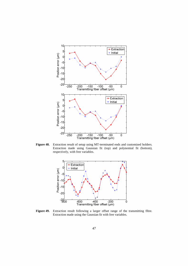
47
Figure 48. Extraction result of setup using MT-terminated ends and customized holders.
Extraction made using Gaussian fit (top) and polynomial fit (bottom),
respectively, with free variables.
Figure 49. Extraction result following a larger offset range of the transmitting fibre.
Extraction made using the Gaussian fit with free variables.

48
Figure 50. Modulation curve measurement for all fibres in the receiving 12-fibre ribbon
using the sensor system setup.
Another field to investigate is differences between the modulation curves for the
cores of the receiving fibre bundle. This will consequently lead to differences in
coupled power to each core which would disturb the parameter fitting in the
extraction routine. Figure 50 shows the modulation curves for all fibres in the
receiving 12-fibre ribbon, following a 4000 µm scan with the transmitting fibre.
Even though the modulation curve shape is the same for the fibres, the maximum
coupled power is clearly different. There are also small differences in the widths of
the curves.
Other contributions to the extraction error are possibly found in the extraction
routine if the modelled field deviates much from the experimental field. In the
following section the impact of different optical fields on the extraction routine is
investigated.
3.6 ANALYSIS OF EXTRACTION PROCEDURE
The response of the extraction routine following different shapes of the optical
field from the transmitting fibre, i.e. different shapes of the modulation function,
was investigated by changing the simulated field in the simulation software.
3.6.1 Shape Variation of the Coupled Power Distribution
In order to test the sensitivity of the extraction routine to deviations in the coupled
power distribution from the modelled one, a number of different shapes of the
optical field were in turn implemented in the hardware description of the simulator.
The field models are listed in Table V below and shown in Figure 51 and Figure 52
respectively. Of special interest is the piecewise linear (PWL) model, where the
slopes and the shoulders of the modulation curve are modelled by two linear

49
functions determined by the radii a and b and the coupled power ratio Ib of Table
V. The piecewise linear field can be written as
22
0 )()( ccb yyxxkI ; (x-xc)2+(y-yc)
2<b
2
I(x,y)= 22 )()( ccaab yyxxkbkI ; b
2(x-xc)
2+(y-yc)
2 a
2 (34)
0 ; (x-xc)2+(y-yc)
2>a
2
where ka=Ib/(a-b) and kb=(I0-Ib)/b. The power distribution P(x,y) is simply given by
multiplying I(x,y) with a scaling factor corresponding to the transmitted power.
Table V. Simulation parameters for test of different optical fields
Field shape Parameter Symbol Value
1 Rectangular Field radius rr 500 µm
2 Triangular Base radius rt 780 µm
3 Gaussian1
Field radius w 500 µm
4 Polynomial2
Radius ra 780 µm
5 Piecewise linear
Outer field radius
Inner field radius
a
b
651 µm
283 µm
Coupled power ratio at r=b Ib 0.88
1-5 - Coupled power ratio at r=0 I0 1
1) According to (31)
2) According to (32)
Figure 51. Simulated rectangular, triangular and piecewise linear (PWL) field shapes
with parameters from Table V.

50
Figure 52. Measured modulation curve with fitted Gaussian and polynomial fields and
manually fitted piecewise linear (PWL) field shape (parameters as in Table
V).
Using the Gaussian model for extraction and a simulated input modulation function
with a rectangular shape, i.e. a constant intensity within the field radius, results in
an extraction result shown in Figure 53. The periodicity of the extraction error
coincides with the core separation of 250 µm, with maximum absolute errors at
offset positions equal to the core positions and minimum errors at positions
halfway between two cores.
A triangular shaped input field is more sensitive and leads to smaller errors as
shown in Figure 54, and a similar behaviour with an even smaller error is shown
for the polynomial input field in Figure 55. The same periodicity pattern as for the
rectangular field can be identified also for the triangular and the polynomial field.
An important observation so far is also that the shape of the input field, and in
reality the agreement between the extraction field model and the real shape of the
coupled input field, is very important for the extraction result.
The piecewise linear (PWL) function shaped field shown in Figure 52 looks
promising for modelling the real input field. The extraction errors using the
Gaussian model on a PWL input field shown in Figure 56 also look very similar to
the behaviour shown in Figure 49, where the Gaussian model has been used for
extraction on real setup images. As in the case of a Gaussian input field and
extraction using the Gaussian model, the extraction error using the piecewise linear
model on the simulated PWL field is consequently very small as shown in Figure
57.

51
Figure 53. Extraction errors using the Gaussian model on a simulated rectangular shape
input field according to Table V.
Figure 54. Extraction errors using the Gaussian model on a simulated triangular input
field shape according to Table V.
Figure 55. Extraction errors using the Gaussian model on a simulated polynomial input
field shape according to Table V.

52
Figure 56. Extraction errors using the Gaussian model on a simulated piecewise linear
input field shape according to Table V.
Figure 57. Extraction errors using the piecewise linear (PWL) model on a simulated
PWL input field shape according to Table V.
3.6.2 Extraction with an Alternative Fitting Function
With the promising simulations using the piecewise linear field model, this
function was implemented in the extraction algorithm and used for extraction of
real setup intensity images. The transmitting fiber was set into 21 positions spaced
25 µm, starting at 0 µm offset and ending at 500 µm offset. To keep better control
of the linear pieces, the inner field intensity Ib was set at a constant value of 0.88.
The extraction errors are shown in Figure 58. A comparison was made with the
Gaussian model as in the previous examples, leading to the extraction errors shown
in Figure 59. Even though the errors are still higher than expected, the tendency of
a more stable and smoother extraction error variation is notable. The results are
promising for further work on this matter.

53
Figure 58. Extraction using a piecewise linear field on real setup intensity images.
Figure 59. Extraction using a Gaussian field on the same images as in Figure 58.


55
4 SUMMARY OF PUBLICATIONS
Paper I and Paper II, dealing with theory and applications of sensors based on
coupling between single fibres, relate to Chapter 2 of this thesis. Paper III and
Paper IV, which concern simulations and experiments on a sensor system based on
coupling to multiple cores using an image sensor for readout, relate to Chapter 3.
4.1 PAPER I
In this paper the modulation function for some standard fibre types is determined
experimentally. Important sensor characteristics such as coupled power and
sensitivity are discussed. Furthermore the impact on the slope of the modulation
curve, also known as the modulation index, for a proposed multiple pass
configuration is investigated. The results are analyzed theoretically using a
Gaussian function for modelling of the modulation curve. It is shown theoretically
and experimentally that to benefit from the multiple pass configuration, reflection
and alignment losses in every pass need to be minimised. This requirement leads to
a more complicated and costly sensor design.
4.2 PAPER II
A practical, industrial application of a coupling based sensor is described. A
bimetal strip serves as actuator for a temperature sensor based on coupling between
a fixed and a movable 62.5 µm core multimode fibre. Using the results from Paper
I, the sensor transfer function is described theoretically and used for designing a
sensor for temperature measurements in the range 130-170 °C. The sensor involves
a two-axis fibre positioning device for calibration purposes. The expected
performance is verified by measurements of the transfer function using a calibrated
thermometer. Furthermore the sensor multiplexing and networking is discussed,
suggesting the OTDR as an effective tool for interrogation of the sensor network
using combined spatial and time division multiplexing. The use of blown fibre and
micro-ducts for efficient and flexible installation of the sensor network is
demonstrated. Measured temperature variations using an installed prototype sensor
is shown to agree well with data logged by the existing conventional process sensor
and demonstrates the suitability of the sensor technique for the application.
4.3 PAPER III
Bearing in mind the alignment issues associated with coupling based sensors in
general, and the experience from the work presented in Paper I, a new design
concept for this sensor family is suggested. The sensor is based on coupling
between a movable, transmitting large core fibre and a fixed, receiving fibre bundle
or multicore fibre, using an image sensor for measurement of the coupled power to
each individual core. Position extraction and calibration are handled by software
routines, and the alignment need is significantly reduced. A simulation tool for the
complete sensor system setup is described and used for simulation of different

56
configurations involving parameters such as fibre type, number and separation of
cores and image sensor pixel size. The modelling of the modulation function is
based on parts of the work in Paper I. The simulations indicate that extraction
errors below 1 µm are possible to achieve with standard fibre and image
acquisition components.
4.4 PAPER IV
Based on the simulations reported on in Paper III, an experimental setup using
standard components is made. The setup involves a 650 nm wavelength LED, a
200 µm core transmitting fibre, a receiving 12-fibre ribbon with standard single-
mode fibres and a 1.3 megapixel CMOS image sensor based network camera. The
position extraction performance using modulation functions based on the Gaussian
model used in paper I and an alternative polynomial function, respectively, is
studied. The resulting extraction error is significantly larger, essentially up to 5 µm,
than the less than 1 µm error experienced in a simulation of the same setup. Two
major error sources are identified: core position instability in the fibre ribbon,
resulting in an error of up to 3 µm, and electronic noise in the image sensor
resulting in an error of less than 1 µm. The electronic noise is the theoretical limit
of the system and also the only noise source that is modelled in the simulator. An
important conclusion is that the receiving fibre bundle cores must be fixed, in this
case for instance by terminating the ribbon ends with connectors. Furthermore the
modulation function model used and differences in coupled power between each
individual receiving core are other suggested important fields for further
investigation.
4.5 AUTHOR’S CONTRIBUTIONS
The author of this thesis has had the main responsibility for all papers included in
the thesis. The author’s specific contribution to each paper is as follows:
Paper I: Main author. Experiments, theoretical parts, results.
Paper II: Main author. Experimental parts, theoretical parts and results.
Paper III: Main author. Simulator programming parts, simulations, results.
Paper IV: Main author. Theory, experiments, simulations, results.
57
5 THESIS SUMMARY
This thesis contributes to the research and application field of coupling based
intensity modulated sensors, but part of the work may also be applied in other
fields within the optical fibre sensing community. Chapter 2 deals with
fundamental theory and experiments, design considerations, referencing and
multiplexing techniques and finally with industrial applications of coupling based
intensity modulated sensors. In chapter 3 a new approach is introduced regarding
sensor design and interrogation, involving simulations and experimental work on
the complete sensor system setup.
5.1 CONCLUSIONS
Intensity modulated fibre-optic sensors based on coupling between fibres
intentionally offer low-cost sensor system solutions in different fields of
application. The interrogation of the sensors is also simple and straight forward,
since basically standard LED and PD components and a minimum of electronics is
required in order to convert the sensor response to an output signal. Interrogation
and networking of the sensors can easily be facilitated with for instance an OTDR
system and a coupler or a switch, creating a hybrid time and spatial division
multiplexed sensor network.
In order to get high coupled power between the fibres in the sensor device there is
however a need for precision alignment of the fibres, causing more expensive
designs, when using standard fibres with small cores. It is shown that efforts to
increase the sensitivity of the sensor by using multiple passes are likely to fail
because of the alignment requirement and the need to eliminate the reflection
losses experienced at each interface.
A design concept for a coupling based temperature sensor for an industrial
application is demonstrated. With the built-in alignment device, precision
alignment can be made and the sensor calibrated to the desired operating range.
This design however makes the sensor more expensive and bulky. The use of an
OTDR for sensor monitoring is proposed as an efficient tool for multiplexing and
referencing of the sensors in the network. As in the communications industry,
blown fibre installation adds effectiveness and flexibility in the installation of the
sensor network.
The alignment issue associated with the coupling based sensors can be significantly
relaxed by using the proposed single fibre to multicore fibre, or fibre bundle,
coupling with image sensor intensity readout. Simulations and experiments on such
a setup indicate a position sensing accuracy down to below 1 µm in theory.
Practical limitations, leading to larger errors, are pointed out to be core position
instability in the receiving fibre/bundle and further discrepancies in the real and
expected modulation function of the sensor setup, also involving differences

58
between the cores in terms of coupled power. The core position instability can
easily be solved by connector termination, while the latter issue needs further
investigation.
In contrast to applications with a position sensitive detector, the proposed fibre to
multicore fibre coupling gives a possibility of a passive position sensing device
since the image sensor and the electronics can be placed away from the sensing
location. Multiplexing of many sensors can be facilitated by allocating different
parts of the image sensor pixel area to different multicore fibres.
5.2 FUTURE WORK
Future work in the subject should be concentrated on the fibre to multicore fibre
coupling setup in terms of investigating the differences in modulation function
between individual cores of the receiving fibre and which impact this has on the
extraction result. Furthermore the curve fitting part of the extraction algorithm
should be analyzed further, with respect to the field model used, in order to
minimize the extraction error.
Once the experimental error is minimized, the sensor concept should be
implemented into a practical application. Such an application could be a position
sensor or a temperature sensor involving a bimetal strip. An interesting problem is
also to optimize the number of receiving fibre cores versus the extraction error and
extraction time.

59
6 REFERENCES
[1] M. Jaaskelainen, “Advances in the Use of Optical Fibers Sensors for Oil
Reservoir Monitoring”, in 18th International Optical Fiber Sensors
Conference Technical Digest (Optical Society of America, Washington, DC,
2006), TuB1, ISBN 1‐55752‐817‐9.
[2] S. Knudsen, G.B. Havsgård, A. Berg, D. Thingbø, F. Bostick and M.
Eriksrud, “High Resolution Fiber-Optic 3-C Seismic Sensor System for In-
Well Imaging and Monitoring Applications”, in 18th International Optical
Fiber Sensors Conference Technical Digest (Optical Society of America,
Washington, DC, 2006), FB2, ISBN 1‐55752‐817‐9.
[3] M. Willsch, T. Bosselmann and O. Beierl, ”3 Phase Optical Voltage Sensing
with Fiber Optical Electric Field Probes in Power Switch Yards”, in 14th
International Conference on Optical Fiber Sensors, Proc. of SPIE vol. 4185,
pp. 230-233, 2000.
[4] A.H. Rose and J.N. Blake, ”Free Form Factor Optical Current Sensor for AC
and DC Commercial Power Applications”, in 18th International Optical
Fiber Sensors Conference Technical Digest (Optical Society of America,
Washington, DC, 2006), FB5, ISBN 1‐55752‐817‐9.
[5] V. Vali and R.W. Shorthill, “Fiber Ring Interferometer”, Applied Optics,
vol. 15, no. 5, pp. 1099-1100, 1976.
[6] G.A. Pavlath, ”Fiber Optic Gyros: The Vision Realized”, in 18th
International Optical Fiber Sensors Conference Technical Digest (Optical
Society of America, Washington, DC, 2006), MA3, ISBN 1‐55752‐817‐9.
[7] ULRICA Distributed Heat Detection System, Product description, Fiberson
AB, http://www.fiberson.se (accessed 2008-11-01).
[8] W. Craig Michie, B. Culshaw, M. Konstantaki, I. McKenzie, S. Kelly, N.B.
Graham and C. Moran, ”Distributed pH and Water Detection Using Fiber-
optic Sensors and Hydrogels”, Journal of Lightwave Technology, vol. 13, no.
7, 1995.
[9] A. MacLean, C. Moran, G. Thursby, S.G. Pierce, B. Culshaw and N.B.
Graham, ”Distributed Fibre Optic Sensors for Humidity and Hydrocarbon
Detection”, 7th International Symposium on Smart Structures and Materials,
Newport Beach, CA, 2000.
[10] A. MacLean, C. Moran, W. Johnstone, B. Culshaw, D. Marsh and P. Parker,
”Detection of hydrocarbon fuel spills using a distributed fibre optic sensor”,
Sensors and Actuators A, vol. 109, pp.60-67, 2003.
[11] J.P Dakin, D.J. Pratt, G.W. Bibby and J.N. Ross, “Distributed optical fibre
Raman temperature sensor using a semiconductor light source and detector”,
Electronics Letters, vol. 21, no. 13, pp. 569-570, 1985.
[12] X. Bao, J. Dhliwayo, N. Heron, D.J. Webb and D.A. Jackson, “Experimental
and theoretical studies on a distributed temperature sensor based on Brillouin
scattering”, Journal of Lightwave Technology, vol 13, no. 7, pp. 1340-1348,
1995.

60
[13] X. Bao, M. DeMerchant, A. Brown and T. Bremner, ”Tensile and
Compressive Strain Measurement in the Lab and Field With the Distributed
Brillouin Scattering Sensor”, Journal of Lightwave Technology, vol. 19, no.
11, pp. 1698-1704, 2001.
[14] C. Menadier, C. Kissinger and H. Adkins, “The fotonic sensor,” Instruments
and Control Systems, vol. 40, pp. 114-120, 1967.
[15] M. Brenci, G. Conforti, A.G. Mignani and A.M. Scheggi, ”Fiber Optic
Position Sensor Array”, Optical Fiber Sensors, 1988 Technical Digest
Series, Vol. 2 (Optical Society of America, Washington, D.C.), pp. 141-144,
1988.
[16] G. Conforti, M. Brenci, A. Mencaglia and A.G. Mignani, “Fiber optic
vibration sensor for remote monitoring in high power electric machines”,
Applied Optics, vol. 28, no.23, 1989.
[17] J.M. López-Higuera, M.A. Morante and A. Cobo, “Simple Low-Frequency
Optical Fiber Accelerometer with Large Rotating Machine Monitoring
Applications”, Journal of Lightwave Technology, vol. 15, no. 7, pp. 1120-
1130, 1997.
[18] B.E. Jones and R.C. Spooncer, “An Optical Fibre Pressure Sensor Using a
Holographic Shutter Modulator with Two-Wavelength Intensity
Referencing”, Proc. 2nd
International Conference on Optical Fiber Sensors,
pp.223-226, 1984.
[19] J.M. López-Higuera, A. Cobo, J. Echevarría, O.M. Conde and F.J. Madruga,
“Temperature, Displacement and Acceleration Fiber Optic Sensor for Large
Machinery Monitoring”, Proceedings of the SPIE, vol. 4328, pp. 142-150,
2001.
[20] K. Toshima, H. Satoh, and M. Kimura, “One-dimensional vibration sensor
using a Si-cantilevercoupled with an optical fiber”, Proceedings of the SPIE,
vol. 3878, pp. 350-357, 1999.
[21] M. Kimura and K. Toshima, “Vibration sensor using optical-fiber cantilever
with bulb-lens”, Sensors and Actuators A, vol. 66, pp.178-183, 1998.
[22] E. Peiner, D. Scholz, A. Schlachetzki and P. Hauptmann, “A micromachined
vibration sensor based on the control of power transmitted between optical
fibres”, Sensors and Actuators A, vol. 65, pp. 23-29, 1998.
[23] E. Ollier, P. Philippe, C. Chabrol and P. Mottier, “Micro-Opto-Mechanical
Vibration Sensor Integrated on Silicon”, Journal of Lightwave Technology,
vol. 17, no. 1, pp. 26-29, 1999.
[24] C.M. Miller, S.C. Mettler and I.A. White, Optical Fiber Splices and
Connectors: Theory and Methods, Marcel Dekker, Inc., ISBN 0-8247-7520-
1, 1986.
[25] B.E. Jones, R.S. Medlock and R.C. Spooncer, “Intensity and Wavelength-
Based Sensors and Optical Acuators”, in Optical Fiber Sensors: Systems and
Applications, B. Culshaw and J. Dakin (eds.), Artech House, Inc., ISBN 0-
89006-376-1, 1989.

61
[26] G. He and F.W. Cuomo, “A Light Intensity Function Suitable for Multimode
Fiber-Optic Sensors”, Journal of Lightwave Technology, vol.9, no. 4, pp.
545-551, 1991.
[27] A. Cobo, M.A. Morante, J.L. Arce, C. Jaúregui and J.M. López-Higuera,
“More Accurate Coupling Function Approach for Optical Transducers Based
on Power Coupling Between Multimode Fibers”, Proc. of 13th International
Conference on Optical Fiber Sensors, pp. 442-445.
[28] A. Cobo García and J. Echevarría Cuenca, “Transduction Techniques Based
on Intensity Modulation of Light” in Handbook of Optical Fibre Sensing
Technology, J.M. López-Higuera (ed.), John Wiley & Sons, Ltd., ISBN 0-
471-82053-9, 2002.
[29] Y. Dong, N. Li, H. Wang, Y. Zhao and G. Wei, “Optical fiber sensor applied
to detect the vibration of electrical machines”, Proceedings of the SPIE, vol.
2895, pp.516-520, 1996.
[30] B. Culshaw, J. Foley and I.P. Giles, “A balancing technique for optical fibre
intensity modulated transducers”, Proc. 2nd
International Conference on
Optical Fiber Sensors (Proceedings of the SPIE, vol. 574), pp. 117-120,
1984.
[31] P. Menke and T. Bosselmann, “Temperature Compensation in Magnetooptic
AC Current Sensors Using an Intelligent AC-DC Signal Evaluation”,
Journal of Lightwave Technology, vol. 13, no. 7, pp. 1362-1370, 1995.
[32] R. Kist, “Point Sensor Multiplexing Principles” in Optical Fiber Sensors:
Systems and Applications, B. Culshaw and J. Dakin (eds.), Artech House,
Inc., ISBN 0-89006-376-1, 1989.
[33] A. Dandridge and C. Kirkendall, “Passive Fiber Optic Sensor Networks” in
J.M. López-Higuera (ed.), Handbook of Optical Fibre Sensing Technology,
John Wiley & Sons, Ltd., ISBN 0-471-82053-9, 2002.
[34] Patent “Fiberoptical Sensor”, International Application Number
PCT/SE2005/000275, International Publication Number WO/2005/080913,
World Intellectual Property Organization, http://www.wipo.int/pctdb/en/
(accessed 2008-11-01).
[35] J. Jason, H.-E. Nilsson, B. Arvidsson and A. Larsson, “Modulation Function
Study of Coupling Based Intensity-Modulated Fiber-Optic Sensors”,
Technical Digest: SOFM 2006, NIST Special Publication 1055, pp. 6-9,
2006.
[36] MT ferrule product description, The Furukawa Electric Co.,
http://www.furukawa.co.jp/connector/mtfer.htm (accessed 2008-11-02).
[37] M. Morante, A. Cobo, J.M. López-Higuera and M. López-Amo, “New
approach using a bare fiber optic cantilever beam as a low-frequency
acceleration measuring element”, Optical Engineering, vol. 35, no. 6, pp.
1700-1706, 1996.
[38] J.M. López-Higuera, A. Cobo, M.A. Morante, J. Echevarría, J.L. Arce, M.
Lomer and R. López, “New low cost fiber optic accelerometer system for
stator winding monitoring of hydroelectric generating machines”,
Proceedings. of the SPIE, vol. 2868, pp. 510-515, 1996.
62
[39] J.M. López-Higuera, M.A. Morante and A. Cobo, “Simple Low.Frequency
Optical Fiber Accelerometer with Large Rotating Machine Monitoring
Applications”, Journal of Lightwave Technology, vol. 15, no. 7, 1997.
[40] Y. Libo and P. Jian, “Fiber-optic temperature sensor with variable-
sensitivity”, Proceedings of the SPIE, vol. 2070, pp. 514-519, 1993.
[41] P.J. Henderson, N.A. Pilling, R. Smith and G.R. Jones, “Optical temperature
probe for extended industrial monitoring”, Proceedings of the SPIE, vol.
2072, pp. 119-125, 1994.
[42] N. Ma, F. Luo and A. Meng, “Intelligent fiber optic temperature measuring
system”, Proceedings of the SPIE, vol. 3541, pp. 125-131, 1999.
[43] J. Jason, F. Sunnegårdh, N. Paulsson, J. Söderberg, J. Hellström and H.-E.
Nilsson, “Fiber-Optic Temperature Monitoring in Pulp Production”,
Proceedings of the 55th IWCS/Focus, pp. 41-49, 2006.
[44] KANTHAL Thermostatic Bimetal, Product Brochure, KANTHAL AB,
Hallstahammar, Sweden .
[45] J. Beller, “OTDR and Backscatter Measurements” in D. Derrickson (ed.),
Fiber Optic Test and Measurement, pp. 442-444, 456, Prentice Hall, Inc.,
1998, ISBN 0-13-534330-5.
[46] P. Lo Curzio, K. Nygård-Skalman and N.-E. Blomdahl, “Cost-effective
Fibre To The Home Broadband Access Installation in Hudiksvall, Sweden”,
Proc. EuroCable 2000, pp. 136-141, 2000.
[47] T. Jendel and P. Lo-Curzio, “Cost Comparison for Air-blown Fibre and
Cable Solutions for a Residential Area”, NOC 2007 proceedings
incorporating OC&I 2007 papers, pp. 75-81, 2007 (ISBN 978-91-633-0869-
7).
[48] J. Jason, A. Larsson, N. Paulsson, K. Nilsson, F. Sunnegårdh, S. Gistvik and
H.-E. Nilsson, “Fibre-to-the-Sensor – Blown Fibre Technology in Fibre-
Optic Sensor Networks”, NOC 2007 proceedings incorporating OC&I 2007
papers, pp. 82-88, 2007 (ISBN 978-91-633-0869-7).
[49] J. Kalenik and R. Pajak, “A cantilever optical-fiber accelerometer”, Sensors
and Actuators A, vol. 68, pp. 350-355, 1998.
[50] A. J. Makynen, J. T. Kostamovaara, and R. A. Myllylä, “A high-resolution
lateral displacement sensing method using active illumination of a
cooperative target and a focused four-quadrant position-sensitive detector”,
IEEE Trans. Instrumentation and Measurement, vol. 44, pp. 46-52, February
1995.
[51] L. Stenberg, The PSD School, Section 1, Sitek Electro Optics AB,
http://www.sitek.se (accessed 2008-11-02)
[52] X. Liu and Y. Gu, “Design of the integrated sensor system for two-
dimensional position based on CCD”, Proceedings of the SPIE, vol. 3897,
pp. 214-222, 1997.
[53] D. Litwiller, “CCD vs. CMOS: Facts and Fiction”, Photonics Spectra,
January 2001.
[54] C.M. Miller, S.C. Mettler and I.A. White, Optical Fiber Splices and
Connectors: Theory and Methods, pp. 103-104, Marcel Dekker, Inc., 1986.

63
[55] J.C. Lagarias, J.A. Reeds, M.H. Wright and P.E. Wright, “Convergence
Properties of the Nelder-Mead Simplex Method in Low Dimensions”, SIAM
Journal of Optimization, vol. 9, pp. 112-147, 1998.
[56] J. Jason, H.-E. Nilsson, B. Arvidsson and A. Larsson, “Monte Carlo
Simulation of the Performance of A Fiber-Optic Position Sensor”, in 18th
International Optical Fiber Sensors Conference Technical Digest
(Optical Society of America, Washington, DC, 2006), TuE48, ISBN:
1‐55752‐817‐9. [57] J. Jason, H.-E. Nilsson, B. Arvidsson and A. Larsson, “Experimental Study
of an Intensity Modulated Fiber-Optic Position Sensor with a Novel Readout
System”, IEEE Sensors Journal, vol. 8, no. 7, 2008.
[58] MT12 ferrule (SM), Product drawing OPC-99098B, The Furukawa Electric
Co., Ltd.