theories of noise and vibration transmission in complex ...jw12/jw pdfs/repprogphys.pdfcertain...
TRANSCRIPT

Rep. Prog. Phys. 49 (1986) 107-170. Printed in Great Britain
Theories of noise and vibration transmission in complex structures
C H Hodges and J Woodhouse
Topexpress Ltd, 13-14 Round Church Street, Cambridge CB5 8AD, UK
Abstract
Theories for analysing the vibrational behaviour of complex structures are examined, parallels being drawn with several other areas of physics in which problems of wave propagation in inhomogeneous media are studied. There are three main stages to the investigation. First, the response to random driving of a single, essentially homogeneous, system is examined. The second, and much more detailed, discussion concerns energy transport between discrete coupled subsystems. In particular, we investigate an approach to this problem which is known as statistical energy analysis. The third main topic is the phenomenon of Anderson localisation as it applies to certain problems of sound and vibration transmission-the phenomenon is much better known in the field of solid-state physics. Applications of it to vibration are of interest in themselves, and also shed light on the theoretical basis of statistical energy analysis, which is a diffusive transport theory.
This review was received in its present form in June 1985.
0034-4885/86/020107 + 64$09.00 @ 1986 The Institute of Physics 107
108 C H Hodges and J Woodhouse
Contents
1. Introduction 2. The response of a homogeneous system
2.1. Preliminary remarks 2.2. Structural response and power input 2.3. Spatial uniformity, equipartition and incoherence 2.4. Statistical aspects of the response
3. Discrete coupled systems and statistical energy analysis 3.1. Background and the conventional justification 3.2. Thermal equilibrium 3.3. The scope of the SEA assumptions 3.4. The stochastic equations 3.5. Wave-mode duality and a little statistics
4.1. Periodic structures and coherent wave theories 4.2. Kinetic theory 4.3. Localisation
5.1. Localisation and SEA
5.2. Localisation and kinetic theory
Acknowledgments References
4. Energy transmission in random media
5. Implications of Anderson localisation for diffusive transport theories
6. Conclusions
Page 109 113 113 114 119 121 125 125 129 131 134 140 147 149 152 154 160 160 164 166 166 167

Noise and vibration transmission in complex structures 109
1. Introduction
The theories we discuss in this review have been motivated by very practical consider- ations. We shall be concerned with problems relating to the understanding of vibration in complex mechanical structures such as buildings, ships and aircraft, and the usual reason to seek such understanding is to control the vibrations. Nevertheless, we hope to convince the reader that such applications can pose theoretical problems which are not without interest. Not only this: it turns out that in tackling such problems the engineer is using or trying to develop approaches which have their counterparts in other areas of physics as remote from engineering as solid-state physics and radio astronomy. What all of these areas have in common is a central concern with the problem of wave propagation in inhomogeneous media and with the fact that the systems under investigation are often too large and complex for a straightforward numerical solution of the relevant wave equation to be possible or very illuminating. It seems therefore that a number of useful insights may be gained from making explicit the parallels with these different areas. We shall note a number of such parallels in this review, and we will draw particularly heavily on the phenomenon of transport of quantum mechanical electrons in disordered solids, but with the application to struc- tural vibration always borne in mind.
The sort of problem we envisage is that of a complex structure subjected to some kind of forcing, for example by machinery or by pressure fields in a surrounding fluid. We wish to try to understand and predict the way in which the structure responds to the forcing, and in particular the way the vibration propagates from a source (e.g. a machine) into distant parts of the system. The object could eventually be to try to localise the vibration in the region of the source as far as is possible so that distant parts of the structure are kept quiet. This might be achieved by mounting a machine in such a way that little energy is put into the structure, adding damping material to absorb the vibration which gets into the structure, or making modifications to the design to inhibit propagation through the structure.
One way of trying to predict vibration levels in a structure of this sort might be described as the ‘brute force’ approach. This consists in calculating the detailed dynamic response of the system to the forcing, usually by way of modal analysis-one calculates the normal modes of the system explicitly and then determines the total response of the system as a sum over modal responses. The normal modes are usually calculated numerically by means of an approach known as finite element analysis. We shall not discuss this approach here; see, for example, the standard text by Zienkiewicz (1977). Essentially the method is to express the elastic and kinetic energies in terms of displacements and their derivatives at a mesh of points covering the structure, and then to apply Rayleigh’s variational principle. For the modes to be well predicted the mesh must be sufficiently fine to describe accurately the variation of modal dis- placement.
The application of such methods to the sort of problem we are interested in has rather obvious limitations, although it is often attempted. The problem is that the engineer concerned with vibration control is often interested in frequencies which lie very far up the modal series of a large complex structure. While the finite element
110 C H Hodges and J Woodhouse
approach is very suitable for predicting the first few modes of such a structure, the accurate description of modes far up the series will involve matrix equations of very large dimensions. If one wishes to predict N modes the dimension must obviously be at'least N. For good accuracy it must in fact be considerably larger than this-the higher modes are never very accurate because of the piecewise construction of the finite element modal displacements.
In any case, the individual modes high up the series become increasingly sensitive to details of the physical structure under investigation, to such an extent that they may be influenced by the deviations from ideal design which inevitably occur in construction. This is related to the phenomenon described in the last paragraph: high modes of the finite element model are sensitive to small details in the modelling, and high modes of the real structure are similarly sensitive to small physical details. Thus the modal pattern predicted from the ideal design may not even be relevant in detail to the actual structure-ship, building or aircraft-as manufactured. Equally, one is unlikely to know the fine details of the vibration source accurately enough to calculate the modal amplitudes excited. What the vibration engineer would therefore like is a method which enables him to understand certain broad features of the vibration distribution and transmission without knowledge of the detailed modal structure or the fine details of the excitation.
The reason that such an approach is often possible is that far up the modal series the modes are dense in frequency, and a source of disturbance will often excite many of them. This may happen because the source is of a broad-band nature, or it may happen even for a narrow-band source if the resonances overlap strongly in frequency. The distribution of vibrational energy through the structure, which is what we are often interested in, is the sum over these modal responses, and it may have a simpler behaviour than the amplitude of individual modes. Thus a detailed calculation of all the excited modes may sometimes give us a vast amount of information we do not really need. However, we should note that, particularly in the case of a narrow-band source, the statistical behaviour must be studied in addition to the average response: as we shall see later, the fluctuations about the average can be large.
Related statistical problems are encountered in many other areas of physics. We can divide these problems into two broad groups, and we will find acoustics and vibration problems in both groups. The first group of problems concerns the behaviour of a single, essentially homogeneous, system. The most obvious example is the classical equilibrium thermodynamics for a gas in a box. The variables of interest are predicted by statistical mechanics without the detailed solution of the microscopic equations of motion. Another example, involving wave phenomena, is the theory of energy levels in nuclei of high atomic number where the large number of nucleons rules out any detailed solution of the quantum mechanical wave equation (Brody et al 1981). Here methods exist which give information about the statistical properties of the large number of energy levels (Porter 1965, Mehta 1967). The same methods are useful in the theory of particles consisting of many atoms but too small to be treated in terms of macroscopic material properties; the energy level statistics of the electrons may be used to deduce the physical properties of such particles (Kubo 1962, 1977).
There are a number of problems in acoustics and vibration which concern the statistics of response in a single homogeneous system. The most highly developed class of such problems is to be found in statistical room acoustics. Analyses have been made both of the average response in rooms (see, for example, Sabine (1964) and Cremer et al (1982)) and of the statistics of the deviations from that average both in

Noise and vibration transmission in complex structures 111
space and in frequency (e.g. Schroeder 1962, Lubman 1968, Waterhouse 1968). Very similar questions arise in the study of structural vibration within a simple system like a flat plate (e.g. Waterhouse er a1 1982, Millot er a1 1984). We discuss some basic aspects of the statistics of response in a single homogeneous system in § 2.
The second general class of statistical problems concerns systems whose properties vary in space, raising the question of transport of particles or wave energy between different parts of the structure. These systems may take the form of discrete coupled subsystems, or of continuous variation which is slow on some appropriate length scale. Examples from classical statistical mechanics are linked boxes of gas at different temperatures, and the continuous generalisation of that problem to heat diffusion. In order to define a local temperature in the latter case, the spatial rate of change has to be sufficiently slow for local thermodynamic equilibrium to be assumed. Such problems occur in many areas of physics and are treated by methods coming under the general heading of ‘transport theory’, usually based on the Boltzmann equation.
Both discrete and continuous problems in this second general class occur in the study of acoustics and vibration. There are a variety of problems concerning the spatial distribution of wave energy or intensity in a random medium, including the effects of the incoherent scattered wave field. These are commonly treated by deriving suitable forms of the Boltzmann transport equation, the approach being described variously as ‘transport theory’ (Ishimaru 1978), ‘kinetic theory’ (Howe 1972, 1973) or ‘radiative transfer theory’ (Chandrasekhar 1960). In all these cases, the aim is to obtain statistical information about the wave field without actually solving the wave equation for individual realisations of the medium. We discuss these problems briefly in 0 4.2.
Acoustical problems involving discrete coupled subsystems will form a major theme of this review. Such problems are met in room acoustics (coupled rooms), but the main area in which they are encountered is in an approach to structural vibration known as statistical energy analysis (SEA). SEA has attracted increasing attention (and a textbook (Lyon 1975)) in recent years, and we give a critical review of the approach here. The basic idea of SEA is to divide up a complex structure into a number of coupled subsystems and to model the energy flow between these in the spirit of transport theory, supposing it to mirror the way in which heat flows between coupled conductors. For the sake of illustration one could take the subsystems of an aircraft to be the engines, wings, fuselage and tailplane, or those of a ship to be the hull, decks, bulkheads and water (though these may not, in fact, be the most appropriate ones to choose for an actual application to real aircraft or ships). One then sets up energy balance equations for these subsystems in terms of their spatially averaged vibration levels, the rate of energy transfer between subsystems, the rate of energy dissipation within each subsystem due to damping and the rate of energy input due to external forces. We discuss SEA in some detail in § 3.
Within our second general class of problems, those involving transport of particles or wave energy, there is another division one can make according to what sort of statistical theory is valid for a particular case. For many of these problems, including those involving wave propagation, the Boltzmann equation approach mentioned above is valid. This approach leads ultimately to particle or wave energy propagation governed by the diffusion equation with the diffusion rate determined by local scattering proces- ses. However, there are some problems involving wave propagation for which the simple approach based on the Boltzmann equation is known to break down. Such problems have been most thoroughly studied in solid-state physics in connection with the transport of quantum mechanical electrons in disordered solids. Problems arise if

112 C H Hodges and J Woodhouse
scattering from irregularities is strong enough, or if the dimensionality of the system is low enough. It can then happen that the effect of interference between back-scattered waves reduces the diffusion constant to zero, and wave energy injected into the system eventually ceases to diffuse and is ‘frozen’ until it is absorbed by damping.
This phenomenon can be viewed at a fundamental level as resulting from a change in character of the normal modes, which no longer extend throughout space but are localised in various parts of the system (Anderson 1958, Mott and Anderson 1978). Such behaviour is known as ‘Anderson localisation’ after its discoverer. Anderson localisation has turned out to be of great importance in solid-state physics for studying the transport properties of disordered solids, for example amorphous or doped semicon- ductors and glasses (Mott and Davis 1979). If the electron wavefunctions in a disor- dered solid are localised there is no long-range transport of electrons and the solid is an insulator (at the absolute zero temperature). There has also been some discussion of localisation in connection with lattice vibrations of solids disordered at a microscopic level (Dorokhov 1982, John et al 1983, Kirkpatrick 1985).
Workers in fields outside solid-state physics seem to be generally unaware of the localisation phenomenon. However, some recent papers have suggested that localisa- tion may be exhibited in a wide variety of other areas of physics: for example structural vibration (Hodges 1982, Hodges and Woodhouse 1983), wave propagation in layered media (rock strata) (Levine and Willensen 1983), water waves over an irregular bottom (Guazzelli and Guyon 1983), sound transmission in an acoustic waveguide (Pendry and Kirkman 1985) and plasma physics (Escande and Souillard 1984).
We discuss localisation in some detail in 0 4.3. It is a subject of interest in its own right, and it also sheds light on some of the questions surrounding the scope of validity of SEA. The most likely areas of direct application to structural vibration concern such things as ships, buildings and aircraft which frequently contain structural components which exhibit some kind of spatial periodicity. Perhaps the most common examples are plates with regularly spaced parallel ribs attached to stiffen them. Other examples might be modern tower blocks, which usually incorporate a substantial degree of periodicity in their construction, and railway lines.
Accurately periodic structures do not really fall within the scope of this review, because in a certain sense they are not really complex but simple, even when large. Their modes of vibration are relatively easy to calculate explicitly using what a solid-state physicist would call the Bloch or Floquet theorem (Brillouin 1946, Ziman 1964), and the need to apply statistical methods does not arise. There are many examples in the literature of the application of Bloch’s theorem to structural vibration- for example, Mead (1970, 1975), Cremer et al (1973), Mace (1980a, b) and Hodges et al (1985a). We give a very brief discussion of such problems in 0 4.2.
However, physical realisations of such structures will never be exactly periodic. There will always be some deviation from the ideal design occurring in construction which will introduce a degree of irregularity-for example, in the spacing of ribs on a plate. Such nearly periodic systems are analogous to the imperfect crystal lattices of the solid-state physicist, and it is in them that effects of Anderson localisation can be very significant. Neither periodic structure theory nor conventional transport theory predicts the behaviour even qualitatively correctly. For a large structure in which irregularities of sufficient magnitude extend throughout (what we may call the case of ‘extended disorder’), it is known that the fall-off in response is, on average (i.e. neglecting statistical fluctuations), exponential with distance from the driving point (Anderson 1958). It is also known that the tendency to localisation is strongest for

Noise and vibration transmission in complex structures 113
systems where the wave propagation is one-dimensional in character. Interestingly enough this is often the case for engineering structures, and not only for textbook examples like point constraints on a bending beam. Wave propagation across parallel ribs on a plate can be viewed as the result of transmission in many channels; each channel corresponds to a different wavenumber parallel to the ribs and can be analysed as a one-dimensional problem. In contrast, one has to search hard for realistic one-dimensional systems in solid-state physics.
Finally, in § 5 , we apply some of the insights from the consideration of Anderson localisation to the questions raised in other sections concerning the scope of validity of diffusive transport theOrieS-SEA and kinetic theory. The conditions are investigated under which diffusive behaviour gives way to localisation, according to the current consensus view. A related issue, also briefly discussed, is the sometimes vital distinction between an ensemble-average response on the one hand and the response of a ‘typical’ member of the ensemble on the other. When these two quantities are different, ensemble-average predictions like those of conventional SEA can be seriously mis- leading.
2. The response of a homogeneous system
2.1. Preliminary remarks
In this section we consider the first of our two classes of statistical problem, that of the response of a single homogeneous system. We work in terms of structural vibration, but most of the results apply directly to other problems of wave motion. The material in this section is both of some interest in itself and forms the necessary groundwork for the later sections on problems involving transport of wave energy through more complex systems. A good deal of this material will no doubt already be familiar in other guises to workers in fields outside acoustics and structural vibration.
There is more than one approach to the theory of structural vibration (in common with all wave phenomena), and it is useful at the outset to recognise a basic division into three general classes. These can be characterised as the ‘waves’, ‘modes’ and ‘rays/ wavepackets’ approaches. All three have advantages for particular types of problem, but sometimes the same result may look very different when seen from these different perspectives. We shall want to be able to switch between the approaches, in order to choose the simplest method for each particular problem. However, there is an element of personal preference here, since most people seem to have a natural tendency to think in terms of one approach whenever possible. This is particularly true for the waves-modes dichotomy, which runs through many areas of physics under a variety of names.
In the ‘waves’ view of the world, one considers travelling waves within the system. Theory tends to start from the differential equation for these waves. Irregularities and boundaries are viewed in terms of scattering and reflection, and when we come to talk of transport between coupled systems later, the natural method of analysis would be in terms of reflection and transmission coefficients at the boundary between systems. In the ‘modes’ view of the world, in contrast, everything is described in terms of the normal modes or standing waves within the system. Variational principles are more in evidence than differential equations. Irregularities may be treated as perturbations to the mode shapes and frequencies. Problems of coupled systems tend to be treated

114 C H Hodges and J Woodhouse
by considering sets of modes to describe the individual systems in some way, then studying the coupling between modes in these sets.
The ‘modes’ and ‘waves’ approaches are both formally valid for all problems. The approach in terms of rays/wavepackets, on the other hand, is a short-wavelength approximation which can be more efficient than either for certain classes of problem, where one can describe the response in terms of travelling wavepackets which retain their integrity, and where interference effects between packets need not be taken into account. The packets then propagate as point-like particles, along geodesic ray paths except when meeting obstacles. This approach leads, for example, to geometric acoustics (e.g. Cremer et al. 1982) and geometric optics (e.g. Jenkins and White 1957). It would be described by a quantum physicist as ‘semiclassical’: in the context of transport theory it leads to the Boltzmann equation and diffusive behaviour as men- tioned in the introduction.
2.2. Structural response and power input
We now introduce some basic formalism to describe the response of a system to external excitation. Consider a structure subjected to a force f( t ) acting at some point x. (For simplicity we give the following discussion in terms of scalar velocities and forces-the generalisation to vectors is easy.) For definiteness, we might think of the structure as being an elastic plate of some shape. The response of the plate to this force consists of waves travelling out from the source to the boundaries, to be reflected back into the plate again. In structural vibration problems one is often dealing with systems which are highly reverberant. This means that there is little attenuation due to damping as the wave propagates in the structure and that the reflection from the boundaries is strong, so that a wave is reflected many times before it is absorbed. The net effect of these multiple boundary reflections is to build up a reverberant field which is more or less uniformly distributed through the plate, and which dominates the original outgoing wave (the direct field), except near the source where the latter can be large (Lyon 1975, Cremer et a l 1982).
We are interested in the velocity response v ( t ) of the structure at some point y which may be different from the driving point x. This response is given by
U( t ) = g ( y , X, t - t’)f(t’) dt’ I‘ where g(y, x, t - t ’ ) is the appropriate Green function, i.e. the velocity response at time t and position y to a unit force impulse at time t’ and position x. Equation (2.1) may be rewritten in Fourier space as
where V ( w ) and F ( w ) are the Fourier transforms of U( t ) and f( t ) and
G ( y , x, w ) = J g ( y , x, t ) exp (-iwt) dt. 0
(2.3)
The quantity G ( y , x, w ) is usually known as the transfer admittance; if y = x, it is known as the driving point admittance.
It is useful to express the response of a highly reverberant structure in terms of the normal modes of the system, cp,(x). These modes are the standing waves created by the strong reflection at the boundaries. Provided the damping is small enough, it is

Noise and vibration transmission in complex structures 115
well known (e.g. Skudrzyk 1968) that the admittance may be expressed as
where w, is the angular frequency of the nth mode. Modal damping is described by a damping factor A,,, which is the relative energy dissipation rate. The modes pn are real and orthogonal and are normalised to give unit modal mass so that
1 c p n ( x ) p m ( x ) u ( x ) dx = a n m (2.5)
where a (x) is the mass density (per unit volume, area or length as appropriate) which enters the expression for the total kinetic energy in terms of the velocity. Equation (2.4) implies a symmetry relation for the transfer admittance
G(Y, x, = G(x, Y, U ) . (2.6)
This important property is a special case of a rather general reciprocal theorem for linear vibration problems, in which damping need not be small (so that the decomposi- tion of (2.4) need not be valid) (Rayleigh 1877, 0 107).
Any general force distribution f(x, t ) can be resolved into modal components:
so that
For the particular case of the point force applied at position x = X,
Equation (2.4) is the acoustic version of the standard decomposjtion of the Green function used in many other fields of physics. However, in acoustics the damping term in the denominator, iwAn, plays a more explicit role than is often the case elsewhere. Damping arises from a variety of physical phenomena, some linear and some non-linear (Snowdon 1968). The linear mechanisms are viscoelastic damping within the material making up the structure (Bland 1960) and radiation damping due to losses from the surfaces of the structure into a surrounding medium. In built-up structures internal damping is also created, and often dominated, by non-linear proces- ses occurring at the boundaries between structural elements, for example frictional forces or gas-pumping at rivets (Maidanik 1966, Ungar and Maidanik 1968, Lyon 1975). Processes of this complexity make damping factors difficult to predict theoreti- cally, and indeed for the non-linear processes representation by linear damping factors can only be an approximation (Heck1 1962). Fortunately, damping is frequently small in practice and the approximation proves adequate for most purposes. One must, however, not lose sight of the fact that approximations have been made, even within the context of linear damping theory (Rayleigh 1877). When quantitative predictions are sought for the vibration of a particular structure, it is usually necessary to determine the effective damping factors by measurement (Snowdon 1968, Lyon 1975).
At this stage it is useful to draw an important distinction between different types of reverberant systems-those in which one can easily detect individual resonances

116 C H Hodges and J Woodhouse
and those in which one cannot. Examples of the two types are shown in figure l (a ) and (6). Figure l ( a ) shows the transfer admittance between two points on a portion of a rib-reinforced steel ring. Many individual modal peaks can be seen, rising sharply some 20 dB above their surroundings. The two curves in figure l (b) , in contrast, show no individual resonances, although there are significant statistical fluctuations including some quite deep nulls at certain frequencies. These response curves were measured in the chapel of Clare College, Cambridge, the two curves corresponding to different driving and observing points. They are typical of the behaviour of a large reverberant enclosure (Kuttruff 1979). One can tell that the peaks here do not correspond to individual modes, since they occur at different frequencies in the two cases. Modal peaks occur at fixed frequencies (although, of course, the peak heights will vary with the driving and observing points).
Which of the two categories a particular system belongs to depends on whether the modal resonances in (2.4) are well separated or not; in other words, on what in acoustics is termed the degree of modal overlap (Lyon 1975). If the resonant width
1 '
700 800 Frequency IHz)
Figure 1. ( a ) Transfer admittance between two points of a rib-reinforced ring, illustrating weak modal overlap. The frequency scale is linear; the response is plotted logarithmically. ( b ) Two examples of the frequency response of a reverberant room (the chapel of Clare College, Cambridge), for two different observation points. The fact that the response peaks fall at different frequencies in the two cases is typical of systems with high modal overlap. The frequency range is narrower than in ( a ) , but is still linear. The vertical scale is the same as in (a).

Noise and vibration transmission in complex structures 117
A,, is small compared to the mode frequency separation Sw then there are clearly separated peaks in the response as in figure l ( a ) . If An is large compared to Sw then several resonant modes contribute to the response at each frequency and the result is something like figure 1 ( b ) .
In room acoustics, except at very low frequencies, one is always dealing with the case of strong modal overlap. In contrast, in structural vibration one is more often dealing with the case of weak modal overlap. The reason is that the modal density tends to be lower in a structure (particularly because structural components like beams and plates have effective dimensionality lower than three), coupled with the fact that damping factors tend to be lower for modes of a structure than for modes of a room.
It should be noted that for systems which are effectively one-dimensional, e.g. bending beams, the degree of modal overlap determines directly whether the system is reverberant or not. First consider the group velocity cg. Since the nth mode will tend asymptotically to look sinusoidal with n half-cycles in the length L of the system, we have Sk- .ir/L so that
cg = dw/dk = SwL/.ir = (.irp)-' (2.10)
where Sw is the modal frequency spacing. For future reference we have also expressed cg in terms of p ( w ) , the specific modal density, i.e. the number of modes per unit frequency, per unit length. (Use of this variable implies an assumption that modal density is proportional to the size of the system.) We see that for such one-dimensional systems, 2.ir/Sw is the round-trip time taken for a wavepacket to travel across the system and back again. Thus the round-trip energy attenuation for such a system is given by exp (-2.irA/Sw) (Smith 1980), where A is the damping factor of modes close to the frequency of interest. If such a system is highly reverberant, i.e. wavepackets cross the system many times before being absorbed, the degree of modal overlap (A/Sw) must be weak; it becomes of the order of unity when the system is on the border of becoming non-reverberant. For systems of higher dimensionality, So is usually much smaller than the inverse of the round-trip time, so that strong reverberation can coexist with strong modal overlap, as is the case in room acoustics (Kuttruff 1979).
The final topic in this subsection is the question of the power input into the structure from an external source. We consider first a structure which is driven at one point x = X by a stochastic band-limited excitation f( t ) . The power input involves the velocity response v ( t ) at the driving point and will therefore be related to the force spectrum and the driving point admittance. The mean power input is
m
I_, ni, = (f( t ) v ( t ) ) = (2.ir)-' Re { G ( X , X , w ) } S ( w ) dw (2.11)
where S ( w ) is the (two-sided) power spectral density of the driving force, i.e. IF(w)l' divided by the length of the measurement time window. Only the real part of the admittance enters the equation because, for a given Fourier component, only the velocity response in phase with the driving force contributes to the average work done.
Let us now suppose that the excitation spectrum S ( w ) is smooth on the scale of the resonant widths of the terms in (2 .4) , as one would expect when the damping is small. Using a standard integral relation one deduces that the power input is (e.g. Lyon 1975)
(2.12)

118 C H Hodges and J Woodhouse
independent of A,,. This formula gives the power input in terms of the normal modes (P,, of the structure. These modes are complicated to calculate and, of course, one of the aims of the theories we are interested in is to avoid determining them in detail. A very simple approximation which achieves this is usually sufficient for practical pur- poses: if we assume that S ( w ) is smooth over a sufficiently wide bandwidth, then the fluctuations in ( P ~ ( X ) average out. Using the normalisation relation (5), one can then substitute for cpi(X) in (2.12) and turn the sum into an integral to obtain
jOm S ( w ) p ( w ) dw (2.13)
in terms of the specific modal density p ( w ) (the modal density per unit length/area/volume as appropriate) and the mass density U. Note that a factor of two has entered (2.13), since S ( w ) was originally defined as a two-sided spectrum.
It turns out that there is a ‘waves’ view of the result we have just derived by a ‘modes’ procedure, which has some physical appeal. Equation (2.13) simply corre- sponds to the power injected byf( t ) into the same system if it were injinitely extended; for example, if our actual system were a finite plate of some complicated shape we would consider an infinite flat plate (Lyon 1969, Skudrzyk 1980). The circumstances under which this is a good approximation have been discussed by Smith (1979b). For the case we have discussed of sufficiently large excitation bandwidth B, the force f ( t ) is significantly autocorrelated only over a small time interval of the order of B-’. If this is less than the time for a disturbance to travel from the source to the boundary and back again, the reverberant field is uncorrelated with the force and does not contribute to the mean input power ( v ( t ) f ( t ) ) . This power then depends only on the direct field, so that the infinitely extended system would give the same answer. The indifference of the power input to the presence or the form of the boundaries, provided these are sufficiently far away from the driving point, results from an invariance property of the Green function which has been discussed in several other areas of physics (von Laue 1914, Zener 1941, Friedel 1954, Kittel 1963, Heine 1980).
For future reference, we should note one particular implication of this argument: the power input will not be significantly changed if we couple our system to others to make a more complex structure. There is also a modal view of this result which we shall require later. Up to now we have been talking about point driving. For a more general force distribution, the power input can be written as a sum over modal contributions. Each of these is determined by the power-spectral density S,, (w) of the corresponding modal force (from (2.8)). For smooth S,, (w) , the power input is given
n,,=;z Sn(wn) (2.14)
U
by
n
which clearly reduces to the point driving result for a modal force given by (2.9). In fact, this result can be significantly generalised: the p,, used in it need not be
the normal modes of the system, but can be any complete set of orthonormal functions. For example, they might be approximations to the modes which are not accurate for numerical reasons, or they might represent modes of separate parts of the system which have been modified by coupling. Provided the excitation bandwidth is sufficiently broad, the power input into each p,, coordinate will still be given simply by $, , (U) .
This follows from an argument given by Woodhouse (1981a): the problem is formally equivalent to point driving of one (P,, coordinate ‘oscillator’, for which the power input depends only on the corresponding mass irrespective of coupling to other ‘oscillators’.

Noise and vibration transmission in complex structures 119
2.3. Spatial uniformity, equipartition and incoherence
Within a reverberant system, it is often the case, to a reasonable approximation, that the intensity of response, averaged over a long time interval, is uniformly distributed in space. Two assumptions are commonly made in demonstrating this, which we shall meet repeatedly during this review and whose failure to be satisfied is responsible for many of the deviations of behaviour from the simplest analyses. In modal terms, these assumptions are:
(i) equipartition of modal energy, so that all modes within the system have the same kinetic energy and
(ii) modal incoherence, so that the responses of two different modal coordinates are uncorrelated over a long time interval.
With these two assumptions, the argument for spatial uniformity is very simple. Write the response as a sum of modal contributions, Zq,(t)cp,(x). To obtain the kinetic energy density, we square, multiply by half the density, and time-average:
I=4 C C a(x)vm(t)v,(t)cpm(x)cpn(x) ( m n
(2.15)
because of modal incoherence. But the kinetic energy of the nth mode is just
En = % d ( t ) ) (2.16)
because our normalisation condition (2.5) means that all modal masses are unity. Thus with equipartition so that all E, are equal to E, say, the kinetic energy density is
I = E C a(x)cp:(x) . n
(2.17)
This sum is independent of x, as follows from modal completeness and orthogonality provided we include in the sum enough modes to cover the length scale over which the uniformity is sought, in other words provided our excitation bandwidth is sufficiently broad. The kinetic energy density is then uniform in space and its value is proportional to the modal energy E. The constant of proportionality is equal to the number of modes in the excitation bandwidth divided by the total volume/area/length of the system (as appropriate). In terms of the specific modal density p, we have
I = BpE (2.18)
a result we shall need later. There are likely to be deviations from spatial uniformity if any of these assumptions
are violated: if equipartition or modal incoherence fails, or if the excitation bandwidth is narrow. The latter of these cases has been discussed by Lyon (1975). The effect of the limited range of wavenumbers associated with the narrow frequency band is to produce a spatial pattern of time-averaged intensity which deviates most strongly from the mean value given above near the boundaries of the system.
Effects of modal coherence and departures from equipartition require more effort to analyse. In general, neither assumption is satisfied. The effect of the mode-shape factors in the decomposition equation (2.4) will produce systematic variations of energy among modes for, say, point driving. Similarly, the excitation will induce correlations between the modes. A broad-band random force applied at a point will produce correlated modal forces on any pair of modes which do not have a node at the drive

120 C H Hodges and J Woodhouse
point. If the modes overlap significantly in frequency, their responses will then be significantly correlated, as we shall see in 0 3.4.
One case in which modal incoherence does occur is where the excitation is extended uniformly (in a statistical sense) over the whole of a homogeneous system and the spatial correlations are short-ranged. Then mode orthogonality will ensure incoherence of the modal forces. This type of excitation has been dubbed ‘rain on the roof’ (e.g. Maidanik 1976); a good example would be a plate excited by a turbulent boundary layer where the correlation length of the pressure fluctuations is small compared with the plate bending wavelength. This type of excitation also guarantees equipartition of modal energies, provided the A,, are all equal (which is often a reasonable approxima- tion within a fairly narrow frequency band). It is thus the form of excitation most likely to produce agreement with simple theories, and we shall use it from time to time to test ideas.
In the absence of equipartition and modal incoherence, the kinetic energy density may still turn out to be spatially uniform over much of the system, except for ‘special’ regions. Such regions may be found close to the source, close to the system boundaries (Elishakoff 1976) or at other positions where the source images reinforce (see below). This uniformity can indeed be demonstrated when a large number of modes are excited, either when the excitation bandwidth or the modal density is sufficiently large (Dowel1 1985)-the effects of fluctuation in modal amplitudes simply average out.
For certain simple configurations of structure, there is an interesting ‘waves’ view of the ‘special’ regions referred to above in the work of Crandall and Wittig (1972), Crandall (1977) and Langley and Taylor (1979). Consider a rectangular elastic plate driven at a point with band-limited random noise. For this simple geometry, the reverberant field can be visualised easily in terms of a rectangular array of image sources extending off to infinity. At a ‘general’ point in the plate, these images add incoherently to give the uniform response described above. Along certain special lines, however, each image can be paired with another at the same distance on the other side of the line. These pairs interfere constructively, leading to an enhancement of the vibration level along these lines. The lines can be readily displayed by a version of the well known technique of Chladni patterns, using sand or some other powder sprinkled on the plate; an example is illustrated in figure 2. (Chladni patterns are more commonly generated by pure-tone driving; here broad-band point drive is used.)
These patterns can be ascribed to the effects of failure of equipartition rather than to modal coherences. This is clear, because the analysis still works in the case of weak modal overlap, and in that case modal coherence effects are insignificant, as remarked above. There is only one rather simple example of spatial non-uniformity arising from coherence effects which we need to note. This arises near the driving point, where from a ‘waves’ point of view we would say that the direct field can dominate the reverberant field. From a modal viewpoint, the direct field is precisely the manifestation of the modal correlations induced by point driving (Lyon 1975,§ 2.4, Smith 1981,1982).
This leads to the final topic of this subsection, the corresponding assumptions in a wave viewpoint to the assumption of equipartition and incoherence. In the usual treatment of statistical room acoustics these two effects are lumped together, in the assumption of what is known as a ‘diffuse field’ (e.g. Kuttruff 1979, Cremer et al 1982). Such a field is spatially uniform, and at each point the incoming waves from all directions are uncorrelated and have equal intensities. When applied to broad-band driving, this is precisely equivalent to equipartition and modal incoherence, as is plausible since both lead to spatially uniform kinetic energy density. A detail which

Noise and vibration transmission in complex structures 121
Figure 2. Chladni pattern for broad-band, random, point excitation of an elastic plate. The driving point is indicated by the dark disc towards the top right. The dark lines indicate regions where the response is higher than average. The regions along the edge of the plate would occur for a free-edged plate of any shape and with any driving point. The ‘tic-tac-toe’ pattern based around the driving point will appear for any driving point on a rectangular plate. The additional diagonal line is special to this case, where a square plate is driven at a point on the main diagonal. Other, weaker, lines can also be discerned, resulting from higher-order coherence effects.
will not concern us greatly here is that the diffuse field concept can also be applied to narrow-band driving, even to pure tones, by describing the incoming waves from different directions as having independent phases rather than as being uncorrelated.
2.4. Statistical aspects of the response
We now turn to the question of the statistical fluctuations of the response, either as a function of frequency or as a function of excitation and observing positions within the system. A related problem, to which we shall return in later sections, is that of fluctuations across an ensemble of different physical systems with common statistical properties.
This question is most pressing for narrow-band excitation of a reverberant system, when the uniform average level discussed above is largely masked: the spatial fluctu- ations in the intensity are of the same order as the mean. This is obviously true for weak modal overlap, when only one or two individual modes are excited, but it is also true for strong modal overlap when many modes are excited (recall the deep nulls in figure 1( b)) (Schroeder 1954, Waterhouse 1968, Lubman 1968, Kuttruff 1979, Cremer et a1 1982). Thus, if one is trying to measure the mean intensity in such a system, for example to deduce the sound transmission through a partition between rooms, several independent samples (either measurement points or frequencies) must be used to give a good estimate. This is an important point to note in applications of SEA, which we

122 C H Hodges and J Woodhouse
discuss in the next section, since that technique deals exclusively with spatially averaged response in subsystems.
Response statistics are best understood in the case of strong modal overlap, particularly in the context of statistical room acoustics. We suppose that for an excitation frequency w, all modes within the damping bandwidth w * A contribute substantially to the sum in (2.4), but with random magnitudes and signs corresponding to the variation in the product of modal amplitudes. The statistics of a sum of this sort were first considered by Rayleigh (1877, 0 42a). The problem is the same as that of a random walk in the complex plane. The probability distribution of kinetic energy density I is given by P ( I ) dI, with
P ( I ) =(I)-’ exp ( - I / ( I ) ) . (2.19)
Experimental data for the distribution of intensity have been given, for example, by Waterhouse (1968), Lubman (1968) and Ebeling et a1 (1982) and show good agreement with theory. These authors have also discussed the statistics of response to multi-tone excitation and multi-point spatial averaging. This is important if one wishes to know how many independent sampling poifits and/or excitation frequencies are needed in order to estimate the mean intensity within a given confidence interval.
For weak modal overlap, the analysis of fluctuations is more complicated. One now has to take into account the rapid frequency variation arising from the resonant denominators in (2.4) as well as the varying modal amplitudes. An interesting approach to the problem of fluctuations in this case is that due to Skudrzyk (1980) and described by him as the ‘mean value method’. This is not a statistical analysis at all: instead, one aims to calculate a mean level and the limits of extreme fluctuations about that mean as functions of frequency for given driving and observing points. For some purposes, this is as much as one needs to know about the fluctuations of response. We shall discuss a somewhat similar approach in the next section, when we deal with the equivalent problem for coupled subsystems.
Skudrzyk’s ‘mean’ level is, in fact, a logarithmic mean, i.e. the line drawn through the centre of a logarithmically recorded response curve. This is the line to which the response tends as the modal damping factors are progressively increased and is also the response of the corresponding ‘infinitely extended’ system (as discussed in the previous subsection) (Skudrzyk 1980). It is thus quite readily calculated for simple systems like plates, rods or cylinders. We now wish to calculate the extreme levels reached by the response, above and below this mean line. In the case of weak modal overlap, we can estimate these very easily simply by considering only the dominant terms from the modal expansion for the admittance, (2.4). To calculate the maximum levels, we need only consider single modes and calculate the maximum height of resonance peaks (using the mode normalisation condition (2.5)).
Minimum levels occur between resonance peaks, and to calculate their depth we can use a two-mode approximation. Two cases must be distinguished. If the product of mode amplitudes has the same sign for both modes, there will be a deep ‘antireson- ance’ between the two peaks. If, on the other hand, they have opposite signs, there will be a shallow minimum between peaks. At the driving point of any structure, it follows that there is an antiresonance between every pair of resonances, a result known in circuit theory as Foster’s reactance theorem (Foster 1929). Conversely, for trans- mission between the ends of a one-dimensional system all minima are of the shallow variety, since successive modes will be alternately symmetric and antisymmetric about the centre of the system, so that the product of mode amplitudes changes sign between
Noise and vibration transmission in complex structures 123
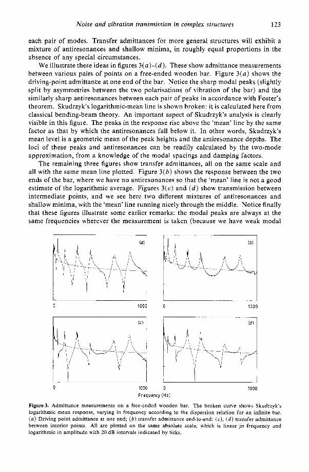
each pair of modes. Transfer admittances for more general structures will exhibit a mixture of antiresonances and shallow minima, in roughly equal proportions in the absence of any special circumstances.
We illustrate these ideas in figures 3( a ) - ( d ) . These show admittance measurements between various pairs of points on a free-ended wooden bar. Figure 3 ( a ) shows the driving-point admittance at one end of the bar. Notice the sharp modal peaks (slightly split by asymmetries between the two polarisations of vibration of the bar) and the similarly sharp antiresonances between each pair of peaks in accordance with Foster’s theorem. Skudrzyk’s logarithmic-mean line is shown broken: it is calculated here from classical bending-beam theory. An important aspect of Skudrzyk’s analysis is clearly visible in this figuie. The peaks in the response rise above the ‘mean’ line by the same factor as that by which the antiresonances fall below it. In other words, Skudrzyk’s mean level is a geometric mean of the peak heights and the antiresonance depths. The loci of these peaks and antiresonances can be readily calculated by the two-mode approximation, from a knowledge of the modal spacings and damping factors.
The remaining three figures show transfer admittances, all on the same scale and all with the same mean line plotted. Figure 3( b ) shows the response between the two ends of the bar, where we have no antiresonances so that the ‘mean’ line is not a good estimate of the logarithmic average. Figures 3 ( c ) and ( d ) show transmission between intermediate points, and we see here two different mixtures of antiresonances and shallow minima, with the ‘mean’ line running nicely through the middle. Notice finally that these figures illustrate some earlier remarks: the modal peaks are always at the same frequencies wherever the measurement is taken (because we have weak modal
0 1000 0 1000
0 1000 0 1000 Frequency (Hz)
Figure 3. Admittance measurements on a free-ended wooden bar. The broken curve shows Skudrzyk’s logarithmic mean response, varying in frequency according to the dispersion relation for an infinite bar. ( a ) Driving point admittance at one end; ( b ) transfer admittance end-to-end: ( c ) , ( d ) transfer admittance between interior points. All are plotted on the same absolute scale, which is linear ,in frequency and logarithmic in amplitude with 20 dB intervals indicated by ticks.
124 C H Hodges and J Woodhouse
overlap), but the antiresonance frequencies depend on the measurement position. The peak heights also vary with measurement position, of course.
As a final aside on Skudrzyk’s approach, we note some recent work by Lyon (1983, 1984). He considered the phase behaviour of the transfer admittance G ( y , x, w ) as a function of frequency and showed how the average rate of phase advance with frequency is given in terms of the proportion of shallow minima to antiresonances in G(y, x, U ) .
His results may be related to Skudrzyk’s analysis of the average of the logarithmic amplitude by a well known result from Fourier transform theory. The Green function g(y, x, t ) is, of course, zero for negative times t and it follows that the real and imaginary parts of G ( y , x, w ) are related by a Hilbert transform (e.g. Morse and Feshbach 1953), the so-called Kramers-Kronig relations. If we think of In G rather than G itself, the same reasoning shows that the logarithmic amplitude and the phase are also related by a Hilbert transform. There is thus a simple connection between this work of Lyon and that of Skudrzyk, although this has not been made explicit by either author.
Skudrzyk’s approach, just described, does not of course amount to a full-blown statistical theory, since it does not attempt to predict the distribution of modal ampli- tudes and frequency spacings necessary to implement the two-mode approximation for a complex structure. Perhaps the best effort to date in that direction is by Lyon (1969), in which he calculates the variance (in frequency) of power input and spatially averaged response for systems of both high and low modal overlap. He does not consider the spatial statistics (discussed earlier, leading, for example, to the Crandall and Wittig patterns). His approach is to assume a statistical distribution for frequency spacings, usually the Poisson distribution, and then to draw on results from the theory of stochastic processes.
In this paper, Lyon also notes that there exists a statistical approach used in other areas of physics which is potentially of relevance in determining the correct distribution of frequency spacings. This approach, known as ‘random matrix theory’, has been used mainly to examine the statistics of level spacings in complex nuclei and small metallic particles. (Energy levels in quantum mechanics correspond, of course, to modal frequencies in acoustics and vibration.)
We illustrate the method briefly by considering the problem of calculating the specific heat of small metallic particles which consist of many atoms, but which are small enough for the discreteness of electron energy levels to be significant. For this discussion, we draw particularly on the recent review article by Brody et a1 (1981), to which the reader is referred for further details. At absolute zero temperature, the electrons fill all the energy states from the lowest up to the Fermi level. At higher temperatures, some electrons will move to excited states above the Fermi level, provided the thermal excitation energy kT is sufficient to overcome the level spacings involved. This is the origin of the contribution of the electrons in the particle to the thermal capacity. If the mean level spacing is substantially greater than kT, such transitions can occur only between states with a spacing much smaller than the mean. Con- sequently, the statistics of level spacings are central to an understanding of the specific heat of the particle.
We consider an ensemble of electrically neutral particles of different shapes and sizes. If the energy levels were spaced independently so that the separations satisfied Poisson statistics, the proportion of particles having a minimum separation across the Fermi level less than kT would be kT divided by the mean spacing. The specific heat would then be proportional to T (Kubo 1962, 1977). However, as was first pointed out by Wigner (1957, see also Porter 1965) in the context of complex nuclei, this result

Noise and vibration transmission in complex structures 125
is modified by the effect of ‘level repulsion’, which makes small level separations less probable than Poisson statistics would imply.
We can describe the effect of level repulsion readily in vibrational terms. Consider a set of oscillators with frequencies randomly distributed about some mean value. Now couple them all together with coupling springs whose strengths are also randomly distributed about some mean value. This coupled system is the prototype for a range of problems, including that of electron energy levels in small particles described above. The level repulsion phenomenon is a familiar one in this context-the effect of coupling two oscillators which were close in frequency is to push those frequencies apart.
The statistics of the modal frequency spacings, in other words of the spacings between eigenvalues of a matrix with both diagonal and off-diagonal elements randomly distributed, can be determined provided one makes certain assumptions about the means, variances and independence of these elements. This is the problem addressed by random matrix theory (Brody et a1 1981). The main conclusion is that the probability of finding small separations E is reduced relative to the independent level model and varies like e n with an integer n > 0 . This leads to a low-temperature specific heat varying like Tntl (Kubo 1977). The value of n depends on a choice of ensemble to which the Hamiltonian matrices describing the individual particles belong; this choice depends on whether there are unpaired electrons on the particles, and on other details discussed by Kubo (1977). For the case where all the matrix elements are real, the prediction turns out to be n = 1 provided the other assumptions of random matrix theory are satisfied.
In fact, the statistical assumptions made in random matrix theory are rather restrictive and it is difficult to think of practical cases where they are a priori satisfied. Even when they are not, the predictions often agree quite well with experiment, as for example the problem of complex nuclei (Brody et a1 1981). On the other hand, there are cases which might seem at a cursory glance to be ideally suited to the method, but for which it can be shown that Poisson statistics are, in fact, appropriate. A significant example is given by the problem of Anderson localisation, which we discuss in § 4. The problem arises from the assumption of independence of all the elements of the matrix: in most practical cases there are interrelations between the elements, and it seems that these may or may not invalidate the conclusions of the theory, depending upon details which to the best of our knowledge are not yet understood.
In consequence, it is not clear to what extent useful applications of random matrix theory can be made to vibration problems. The physical effects of level repulsion certainly apply to many problems, however, and in such cases, random matrix theory provides a possible approach to incorporating these effects into a proper statistical theory built on Skudrzyk’s approach or on the high-modal-overlap room acoustics approach. Any more complete statistical treatment would be even harder, so it is certainly the most appropriate first recourse (Lyon 1969). More effort in this direction would perhaps be merited.
3. Discrete coupled systems and statistical energy analysis
3.1. Background and the conventional justification
Statistical energy analysis attempts to apply a version of simple, diffusive, transport theory to a rather wide class of vibration problems. In a typical application, one would have some source of noise (such as air conditioning plant or engines) in one part of

126 C H Hodges and J Woodhouse
a complicated structure, and one would be trying to control the level of vibration produced at a distant site, for the benefit of sensitive equipment or the comfort of human occupants. To model the flow of vibrational energy from the source to distant parts, one has to take account of at least some of the complexity of the structure, since in general there will be several transmission pathways. SEA is the natural and simplest way of attempting this: the structure is viewed as a set of coupled subsystems and we only consider the spatially averaged vibration level within each subsystem. The energy flow between subsystems is treated using a type of statistical approach which, as we have outlined in the introduction, is common to many areas of physics. Heat diffusion is the clearest analogy.
In order to use such a treatment one has to identify a variable which plays the role of temperature and hence governs the rate of energy flow between subsystems. SEA is usually formulated in terms of the coupling of oscillators which represent modes belonging to different subsystems. (We discuss later the corresponding ‘wave’ view- point.) It is argued (Lyon 1975) that the average energy per oscillator in the subsystem (the average ‘modal energy’) defines its temperature T since in classical statistical mechanics each mode has energy kT Of course, the analogy between the engineering problem and statistical mechanics is not complete. In the latter case ergodicity and the Boltzmann distribution play a central role and these result from small but important non-linearities in the equations of motion. For the sort of problems we shall be considering non-linearity is not of any importance and the modal amplitudes are not, in general, Boltzmann distributed-they are ultimately determined by the external forces, as we have already seen for the case of a single subsystem. There are indeed some subsystems for which ergodicity can be shown to hold, as discussed in an interesting series of articles by Joyce (1975, 1978, 1980), but space does not allow a discussion here.
It is sometimes said that SEA is just a matter of correct energy bookkeeping. All one has to do is to write down for each subsystem equations balancing the power input due to external forces, the power dissipation due to damping and the energy flow to neighbouring subsystems. The diffusive theory enters via an assumption (which we shall discuss in some detail below) that the energy flow between two subsystems is simply proportional to the difference of mean modal energies of those subsystems. This leads to a set of energy balance equations which it is usual to write in the form
where ER and E, are the modal kinetic energies in the subsystems R and Q, averaged over an excitation band whose centre frequency is W. The energy input due to external driving is IIR,in and was discussed in the previous section. NR is the number of modes excited in subsystem R, and the factor of two preceding it arises from our use of kinetic energy rather than total energy as a prime variable. The coefficient of proportionality for the energy flow, a kind of heat conductance, is expressed in terms of a dimensionless ‘coupling loss factor’ T~~ Similarly, the dissipation within subsystem R is described by a dimensionless dissipation loss factor T ~ : in terms of our previous notation, W v R corresponds to the mean value over the subsystem R of the modal damping factors A, within the excitation band. The coupling loss factors obey a reciprocity relation
since the energy lost by R to Q is the energy gained by Q from R. From a knowledge

Noise and vibration transmission in complex structures 127
of the energy input rates, loss factors and coupling loss factors, (3.1) can then be solved for the unknown coupled energies ER.
In the rest of this section we tackle what is really the central problem in SEA, namely the justification of the form of the energy flow between subsystems used in (3.1), and the determination of the coupling loss factors vR,. (No great problem arises in connection with the validity of the other assumption implicit in (3.1), regarding the form of dissipation within each subsystem. We have already discussed dissipation briefly in 5 2.2.) In the remainder of this subsection we outline the usual derivation of the proportionality relation, which has rather restricted validity. In later subsections we examine the steps of the derivation in more detail to determine the scope of validity of that relation and to see what would be needed to improve on it.
The starting point of SEA theory is the simple but remarkable result that, averaged over a long time interval, the mean energy flow between two coupled oscillators (in isolation) driven by suitably random uncorrelated forces is proportional to the difference in their mean energies (e.g. Lyon and Maidanik 1962, Ungar 1967, Newland 1968, Lyon 1975). The constant of proportionality depends on the frequencies of the two oscillators and on the coupling parameters. It is surprising that a result which appears to have its origin in statistical mechanics should apply to a system as simple and small as this! Unfortunately similar exact results for the energy flow between more than two coupled oscillators or modes do not exist in sufficiently simple form to be of much use except for ve special cases, for example identical coupled oscillators (Scharton and Lyon 1968, Woodhouse 1981a).
In consequence, to make use of the two-oscillator result to learn something about coupled subsystems with many degrees of freedom, the usual SEA procedure is now to apply a set of rather sweeping assumptions which enable us to generate simple statistical predictions. We describe each subsystem by a set of generalised coordinates which are the normal modes of that subsystem when isolated from the other subsystems by letting the appropriate coupling parameters tend to zero (known as ‘blocked modes’ (Lyon 1975)). These coordiiiates are analogous to the two oscillators of the original calculation and with the coupling restored we can use the result of that calculation to describe the rate of energy flow between a given coordinate of one subsystem and one coordinate of another subsystem.
We first suppose that each subsystem is driven with band-limited white noise having a flat spectrum between frequencies 6 - B/2 and 6 + B/2, the bandwidth B being large compared with the damping bandwidth of individual modes. Next, for each subsystem we make the two assumptions discussed above in § 2.3: modal incoherence and equipartition. In particular, suppose all modes within the excitation band in subsystem Q have energy E,. This means that the total energy flow into coordinate q of subsystem Q is given by summing over coordinates r of subsystem R whose resonant frequencies lie within the band of excitation. Thus the total energy flow nRQ from subsystem R to subsystem Q within this frequency band is approximately
summing over modes q of subsystem Q lying within the excitation band, where arq is the proportionality constant from the two-oscillator calculation for energy flow between coordinates r and q.
This is of the required form for (3.1), provided we can approximate the double sum over the a in a usefully simple way. The details depend on the precise functional

128 C H Hodges and J Woodhouse
form of arq, which in turn depends on the type of coupling assumed, but in outline the usual approach is as follows. We assume that the frequencies of resonance of the two subsystems are independent random variables, uniformly probable (in an ensemble- average sense) over the band in question, with specific densities p R and pQ, respectively, and then approximate the summations in (3.3) by integrals to give
~ R Q - P R v R P Q v Q ( E R - E Q ) [l wq) dwrdwq (3.4)
where we now regard a as a continuous function of wr and wq, and both integrals are over the band centred on 3 with width B. VQ is the total volume/area/length (as appropriate) of subsystem Q. Finally, under our approximations we can replace all occurrences of w, and wq in the expression for cyrq by (5, except where it appears as the difference w, - wq. At least for many of the types of coupling usually assumed, the integrals can then be calculated straightforwardly to obtain the desired expression for the coupling loss factor (Ungar 1967, Cremer et al 1973, Lyon 1975)-the double integral in (3.4) turns out to be proportional to the bandwidth B for these simple cases (Woodhouse 1981a).
The argument just given will obviously not apply in detail to most practical situations, because of the various assumptions made. This has sometimes meant that when an experimenter has tried to apply SEA to a particular problem and has not obtained sufficiently accurate predictions, the blame has been laid entirely on shortcom- ings in the basic theory. Before we start a more detailed examination of that basic theory in the next subsection, therefore, it is worth considering the various possible causes of ‘wrong’ answers from a SEA model. One possible reason is indeed in the theory. We have made four important assumptions: about equipartition of energy among modes in a subsystem, about incoherence of various contributions enabling us to add energies, about the applicability of the two-oscillator result in the presence of more oscillators and implicitly about the behaviour of certain ensemble averages. In order to fill in the details, we would also have to make assumptions about the form of intermodal coupling, and indeed about precisely how the separate subsystems are to be defined. The four main assumptions listed above can each fail under some circumstances and we shall discuss them all. Limitations of space prevent us addressing the other issues concerning forms of coupling and so on, but these have been discussed in the literature (e.g. Karnopp 1966, Lyon 1975, Woodhouse 1981a).
However, we should recognise two other general reasons why the predictions of a particular SEA model might prove unsatisfactory. The first is that the very generality of SEA makes for complication in applications. Subsystems can be of many different kinds-simple sections of plate or beam, more complicated built-up substructures, enclosed air spaces, even special subsets of modes within a particular structure which it is either necessary or desirable to treat separately (for example, bending and compressional modes in a plate). This in turn means that coupling can take a great variety of forms, so that in practice coupling loss factors can only rarely be calculated and more usually need to be measured. Such measurements themselves are by no means easy-some suggested approaches have been discussed by Ungar and Koronaios (1968), Lyon (1979, Brooks and Maidanik (1977), Bies and Hamid (1980), Woodhouse (1981b) and Craik (1982, 1983), among others. This complication in determining the model parameters is perhaps what makes SEA less universally useful than’ its cousins in diffusive transport theory in other areas of physics. Obviously, if the coupling loss factors are not determined with sufficient accuracy, predictions of the SEA model will

Noise and vibration transmission in complex structures 129
be poor. However, we should recognise that for such complicated systems no other method of calculation of the vibrational behaviour holds out much hope of success either!
One particular type of complication should perhaps be singled out here as being somewhat special. If we have a fluid-loaded structure, we must either treat the unbounded fluid as a subsystem or incorporate it somehow in our description of the coupling between structural subsystems and subsystem damping factors. Neither option is easy. In the first case, we have an extreme case of a non-reverberant subsystem. In the second case, we have in general a hard problem in calculating the coupling between each pair of subsystems, best approached by a wave method (Crighton 1984).
The final general reason why a particular SEA model prediction may be felt unsatisfactory concerns statistical fluctuations. The SEA response estimate is an ensemble average over systems which are different in detail. It may be that a SEA
model will give a perfectly correct prediction of this ensemble average, but that the fluctuations of actual response among members of the ensemble make this estimate not very useful. As well as predicting the average response, we would also like a measure of these fluctuations so that we know how close our actual system should be to the ensemble average. This issue will be taken up in 0 3.5.
There are, in addition, some rather subtle problems associated with ensemble averaging, which we shall consider in 0 5. Some insights gained from the consideration of Anderson localisation in 04.3 will lead us to question the strategy of ensemble- averaging the coupling loss factor as the usual argument demands. Really, one should be ensemble-averaging the response and when the modal overlap is not strong this leads to different answers which reproduce, qualitatively at least, the phenomenon of localisation within a SEA model. However, this is not the end of the story. We will also have discovered in the course of § 4.3 that a linear ensemble average is not always the most appropriate thing to calculate. If one wants the response of a typical member of the ensemble, as we surely do, it is at least sometimes more appropriate to use a logarithmic ensemble average. Doing this allows a SEA model to agree quantitatively with localisation theory in the case of low modal overlap, but not without raising other problems, which we discuss.
While these issues concerning averaging must wait until we have discussed Anderson localisation, we can deal straight away with the other three of the four main assumptions mentioned above. We follow a similar sequence to the discussion of a single system in 0 2. We first discuss a simple result arising from the assumptions of modal equiparti- tion and incoherence within the subsystems. We then discuss in modal terms and in wave terms some of the causes and consequences of failure of either or both of these assumptions in coupled systems, and the scope of applicability of the two-oscillator energy flow result in multimodal systems.
3.2. Thermal equilibrium
We commence our examination of the validity of SEA by demonstrating that for a set of oscillators driven by random uncorrelated forces, equipartition of oscillator energies implies no net energy flow between any subset of these oscillators and the rest of the system. We apply this to energy flow between coupled subsystems by regarding the blocked modes (see above) of the separate subsystems as oscillators. Thus equipartition means that any subsystem is in ‘thermal equilibrium’ with its surroundings. There is also a rather stronger version of this result, which says that under the stated conditions,

130 C H Hodges and J Woodhouse
the energy flow between any pair of subsystems is zero. However, it will turn out that we only need the simpler form, which is very easy to prove and we do not prove the stronger form. (It can be done by the methods we discuss in 0 3.4.) This result is one of the few simple, exact ones which can be established for the case of more than two oscillators. It relates to the discussion in § 2.3 of how modal equipartition and incoherence lead to spatial uniformity of the response: it says that if both these conditions are satisfied within each subsystem separately, then equality of the subsystem modal energies corresponds to thermal equilibrium between each pair of subsystems. As a by-product of proving it, we shall demonstrate the validity of the SEA energy flow result for the important case of weak coupling.
We first express the average oscillator kinetic energies in terms of the spectrum of driving forces and the admittance matrix of the system, described in blocked-mode coordinates. This method appears to have been first used by Ungar (1967) to derive the energy flow relation for two weakly coupled oscillators. By the assumption of incoherence, there are no cross-correlations between the responses to each force acting separately and we can obtain the net response intensity by adding the energies when each modal force acts in turn. Consider a set of oscillators q, r, . . . , driven by such forces, with spectra
where the sum over
S,(w) , $ ( U ) , . . . . The oscillator kinetic energies are given by
Eq =:(U’( t ) ) = (47r-’ A,$, (3.5) r
r includes all oscillators, and CD
Aqr = I_, lGqr(w)l* dw =Arq (3.6)
because of reciprocity (Ungar 1967, Lyon 1975, Woodhouse 1981a). It has been assumed that the spectra & ( U ) and Sr(w) are flat and equal to S, and Sr in the frequency range where Gqr(m) is large. (This range is assumed to encompass the normal-mode frequencies of the coupled oscillators.)
Now the net energy outflow from a subsystem Q into its surroundings is the energy absorbed in the rest of the system when only Q is driven minus the energy absorbed by Q when the rest of the system is driven. When oscillator q (in subsystem Q) is driven, the energy absorbed by oscillator r (in ‘subsystem’ R, the whole of the rest of the system) is equal to twice its kinetic energy times the damping factor A p The kinetic energy of oscillator r is determined by the transfer admittance Gqr(u) from the driven oscillator q to oscillator r, cf (3.5) and (3.6) above. By making the same argument when r is driven and then adding energy flows we deduce the net flow from q to r, and hence from Q to R by summing over q in Q and r in R (Woodhouse 1981a):
n,, = ( 2 ~ 1 - l 1 Aqr(ArSq - A q s r )
= ( 2 / ~ ) EIAqrArAq(eq-er) (3.7)
ep = Sp/4A,. (3.8)
q r
where
A sufficient condition for thermal equilibrium is evidently that ep should be the same for all oscillators p = q, r. Slightly less obviously, it is also a necessary condition since the argument must apply to any partition of the complete system into two subsystems. The ratio ep is, in fact, the energy of oscillator p subject to the same force
Noise and vibration transmission in complex structures 131
but in the absence of coupling, as is seen by equating the power input for an isolated oscillator (cf (2.14)) to its power dissipation. As a result, (3.7) tells us that the energy flow is proportional to the difference in the uncoupled oscillator energies, which has sometimes been taken as the statement of the SEA energy flow relation (Davies 1973, Lyon 1978). However, this is not in keeping with the heat conduction analogy (Smith 1979a); for that analogy, we must relate the energy flow to the energies in the coupled state, and this we now do.
If the coupling is sufficiently weak the uncoupled energies are in any case close to the coupled ones. In that case, (3.7) shows that the total energy outflow from a subsystem is in the form assumed in SEA (see (3.3)). It also gives the coupling proportionality constant in terms of the transfer admittance in blocked-mode coordin- ates. This corresponds exactly to the result for weak coupling given by Woodhouse (1981a), derived by a slightly different route.
Under conditions of thermal equilibrium the coupled and uncoupled oscillator energies are exactly equal. Thermal equilibrium means that the power input into each oscillator is dissipated in that oscillator and its energy is therefore equal to this power input divided by the dissipation factor as in the uncoupled case. As we have already noted, at the end of § 2.2, the power input for broad-band driving depends only on the spectral intensity of the driving force and is the same with or without coupling. Thus the coupled and uncoupled oscillator energies are the same and both are equiparti- tioned. We have proved that thermal equilibrium implies equipartition of oscillator energies. The converse is true because there is a one-to-one correspondence between the spectral intensities of the driving forces and the oscillator energies. (By using the modal expansion (2.4) in (3.6) and performing the frequency integration, it may be verified that the matrix A is always positive definite and thus always has an inverse, except for the uninteresting limiting cases of all damping going to zero or of infinitely tight coupling.)
It is instructive to examine the thermal equilibrium result briefly from the ‘waves’ viewpoint. Thermal equilibrium now corresponds to a balance of total energy fluxes crossing the coupling between a pair of subsystems in each direction. To relate this to the equipartition of modal energies, we need to recall a result from § 2.3 that the kinetic energy density in a diffuse field is proportional to the product of modal energy and specific modal density (2.18). Thus modal equipartition means that the kinetic energy densities in the subsystems on either side of a coupling must be in the same ratio as the specific modal densities of the two subsystems. For one-dimensional subsystems, we can make the link with energy fluxes particularly easily. We have already noted in § 2.2 that for a one-dimensional system the specific modal density is inversely proportional to the group velocity (2.10). Thus the kinetic energy density divided by the modal density is just the energy flux, and this is the quantity correspond- ing to modal energy. For systems of higher dimensions, the relationship is less simple because the directional. dependence of energy flux around the coupling must be taken into account. Of some interest in this connection is the discussion by Weaver (1982, 1984).
3.3. The scope of the S E A assumptions
In this subsection, we investigate in qualitative terms the circumstances under which three assumptions made in the conventional SEA argument in § 3.1 break down and the features of the behaviour when such breakdowns occur. In the next subsection,

132 C H Hodges and J Woodhouse
we will show how to calculate some aspects of that behaviour quantitatively. The three assumptions are: equipartition of modal energies within each subsystem, incoherence of all modal responses and the continued applicability of the two-oscillator energy-flow result in multimodal systems. We discuss these in turn.
Of course, when one looks at a system and wonders whether a SEA model should be appropriate, one does not think immediately in terms of these assumptions. The aspects of behaviour for which one has a more direct insight are some measure of the strength of coupling between subsystems, the degree of reverberance and modal overlap within each subsystem and the nature of the driving forces. One aim of the discussion in this subsection is to relate these concepts, at least qualitatively, to the basic assump- tions of SEA. Broadly speaking, SEA works best with weak coupling, reverberant subsystems but with high modal overlap, and broad-band driving distributed over subsystems. Departures from these ideal conditions produce failures of our basic model assumptions. Again, broadly speaking, stronger coupling tends to require corrections to the two-oscillator result, systems not strongly reverberant violate the incoherence assumption, low modal overlap produces strong departures from equiparti- tion and problems with statistical averaging and details of the force distribution are responsible for a combination of coherence effects and equipartition failures.
There are two qualitative remarks about equipartition which it is useful to make at the outset. First, substantial failures of equipartition within subsystems will indeed prevent a SEA model from working well, but they may indicate a poor choice of subsystems when constructing the SEA model. As mentioned briefly in 0 3.1, it is sometimes necessary to allow for groups of ‘special’ modes within a given structure as separate subsystems for precisely this reason (see e.g. Lyon 1975). Some of the possible candidates are groups of modes with significantly different damping factors from the rest (e.g. Maidanik 1974, Maidanik and Tucker 1974), modes with different physical character (e.g. flexural and compressional modes within a beam or plate) and modes which are in some way concentrated near a boundary between structures, which can have a disproportionate influence on the energy flow across that boundary.
The second general remark about equipartition is simply to note how rarely it will ever be strictly realised. We have already noted that for a single system with equal modal damping factors, rain-on-the-roof driving (which is sometimes a reasonable physical model) produces equipartition. However, for coupled subsystems, even with rain-on-the-roof driving in one subsystem, the responses in the non-driven subsystems will not exhibit equipartition in general: blocked subsystem modes with a higher weighting in the coupling regions will respond more to driving through the coupling. Fortunately, equipartition failures do not necessarily give serious problems. One can work entirely with the mean modal energy and still derive the SEA result, provided the energy differences between oscillators are not correlated with the proportionality constants apq. (Such correlations might not at first sight be expected, although we shall later describe a case where they are significant.) One can also dispense with the assumption if one is prepared to carry out energy-balance calculations at the individual oscillator level, but this brings extra statistical problems (especially in the weak-modal- overlap case, when equipartition failures are most marked). We defer our main discussion of this problem until Q 5.
In due course, we shall calculate the simplest corrections to the SEA energy-flow result which allow for modal coherences and equipartition failures induced by the forcing and the coupling. This discussion of the influence of these two factors on energy flow between subsystems is a natural continuation of our earlier discussion of

Noise and vibration transmission in complex structures 133
their effect on the spatial distribution of response in a single system in 0 2.3. It will turn out that coherence corrections only become significant when subsystems are on the verge of becoming non-reverberant-we have already indicated that if our system contains any such subsystems then strong effects of modal coherence are to be expected.
Non-reverberant subsystems can be important either if they are directly driven, so that the response in the region of the coupling to other subsystems is influenced, or if they appear as links in a transmission pathway to distant parts of the structure (Maidanik 1981a, b, Maidanik and Maga 1981). Opinions differ on the extent to which it is possible to allow non-reverberant systems in something like a SEA model. They depart significantly from the philosophy of SEA, since they bring in variables not previously present-in particular, the position of driving and coupling points withip subsystems. On the other hand, such systems can be very important in practice, especially when efficient damping treatments are available to apply to parts of a structure. The noise-control engineer has to have some way of assessing the perform- ance of such treatments, for example, and it has been argued that an extension of SEA
is the best way to do this (Maidanik 1981a). However, we do not pursue this issue here since our main aim is to assess SEA as an example of transport theory, not to provide a comprehensive guide to noise-control engineering.
We now turn to the scope of validity of the two-oscillator energy-flow result in more complicated systems. This brings in a new qualitative type of behaviour, and to introduce it and motivate our investigation we look again at (3.7) from the previous subsection. This showed that, provided the modal forces are incoherent, the total energy flow between a subsystem and the rest of the system is a sum over differences of uncoupled modal energies. If we make the same proviso about force incoherence (since we shall deal separately with force-coherence effects), this total energy outflow will also be a linear combination of the actual energies of the blocked-mode coordinates in the coupled state-this is made clear by inverting (3.5) and substituting for Sq and Sr in (3.7). Thus
with some set of coefficients cp Moreover, to be consistent with the thermal equilibrium result of the last subsection we know that the coefficients cp must sum to zero, so that there is no energy flow when all modal energies Ep are equal.
It is intriguing to note that the terms in such a linear combination can always be rearranged into a form closely analogous to (3.7), in which, however, the energy differences are those (Eq - E r ) in the coupled state:
(3.10)
with some matrix Zq, where the sums over q and r are restricted to subsystems Q and R, respectively. (This follows directly from the condition Zcp = 0.) The matrix Z,, is by no means uniquely specified by this operation, so one must be wary of making any physical interpretation of the individual terms in the sum. However, because of the similarities with (3.7), it clearly reduces to the weak-coupling case we have already discussed in the appropriate limit.
At first glance, (3.10) seems to justify the SEA energy-flow relationbin this case with no further ado (compare the discussion by Woodhouse (1981b)). However, it does not show that SEA as usually understood always applies in this case. In whatever way we carry out the rearrangement of (3.9) in detail, (3.10) will contain terms which

134 C H Hodges and J Woodhouse
correspond to what we shall call ‘indirect coupling’. These are terms in the sum (3.10) involving energy differences between blocked-mode oscillators which are not directly coupled together-while such terms are acceptable in (3.7), they are not compatible with the simple picture of the diffusion analogy in this case. No work can be done by one oscillator on another without a direct connection between them. In the next section, we shall show that such indirect coupling arises naturally in an analysis in ascending powers of the coupling strength at higher order than the direct coupling. It will turn out to occur most strongly in the context of what in quantum mechanics would be called tunnelling behaviour and it will also turn out, in at least one interesting case, to have a simple physical interpretation.
Indirect coupling is an effect of the failure of the two-oscillator energy-flow result: when we go beyond weak coupling, the energy flow between two oscillators is influenced by the energies of all the other oscillators in the system. If we then try to build up this oscillator description into a subsystem by the kind of argument used in 0 3.1, indirect coupling will remain a problem. If the coupling is not sufficiently weak, there will be significant terms involving energy differences between subsystems which are not directly coupled.
There is one final general remark which should be made before we get down to details in the next subsection. We are going to consider the corrections to the simplest SEA modelling which occur when the coupling between subsystems ceases to be sufficiently weak and/or when the effect of correlations induced by the driving have to be taken into account. It should be recognised from the outset that if it is necessary to calculate such corrections in a given application, then much of the point of SEA
modelling has been lost. The results to be given here should be regarded primarily as giving useful qualitative information about the expected circumstances and form of deviations from the simplest SEA predictions, which can guide the formulation of SEA
models and help in the interpretation of measurements. Some attempts have been made to broaden the formulation of SEA to include, for example, non-reverberant subsystems (Maidanik 1981a). As mentioned above, we do not pursue these here since our aim is to discuss SEA as theory, not noise control as engineering.
3.4. The stochastic equations
In 3 3.2, we have verified the SEA energy-flow relation, at least for the case of weak coupling, and we have seen that one way to calculate the energy-flow proportionality constant is from the admittance matrix in blocked-mode coordinates. This matrix in turn can be calculated in terms of the coupled modes of the whole system (Woodhouse 1981a). One can then calculate the coupling loss factor for this case, by carrying out a frequency integral and following the procedure outlined in 8 3.1. While this admit- tance matrix approach could be pursued further to investigate the effects of stronger coupling and so on, it seems a rather perverse way to go about things. Once one has calculated the admittance matrix to the desired accuracy, one can calculate the response to driving without ever using the SEA model! This does not prevent the method yielding useful conclusions of a general nature, and indeed the results we shall derive here could probably be found that way. However, it seems slightly preferable to use a different approach.
One possibility, which we now consider, is the ‘stochastic equation’ approach used by Lyon and Maidanik (1962) in one of the first papers describing what later became known as SEA. Although this method was one of the first used to study energy flow

Noise and vibration transmission in complex structures 135
among coupled oscillators, it has received little attention since, and perhaps the method has not been exploited to the full for investigating modal coherence and energy-flow relationships. The stochastic equation approach gives a general method of transforming a coupled-mode problem into a problem involving only energy variables and details of the driving and this is of some interest independent of the utility of the results derived.
As in the previous two subsections, we are discussing energy flow between subsys- tems from the ‘mode-coupling’ point of view, so that we model the dynamical behaviour of the structure by a set of coupled oscillators, each oscillator corresponding to a blocked mode of a subsystem. We may write the resulting equations of motion as
W p + A p W p + + ~ ~ p = - C p , ~ , + & ( t ) 4’P
(3.11)
where wp is the amplitude of response of the pth blocked-mode oscillator, dots denote time derivatives and wp and A, are the modal frequency and damping factor as before. We illustrate the method for the simplest case, spring-like coupling Cp,w,. It can be extended to cope with other types of coupling, but as mentioned earlier, space does not permit a detailed discussion of coupling mechanisms here.
To derive the stochastic equations we multiply each of the N equations (3.11) by the variables w, and w, in turn ( r = 1 , N ) and take the time average. The resulting equations, 2 N 2 of them, are expressed in terms of unknown modal correlation functions (wrkP), (wrwp) , (wrwp) , etc, which we would like to determine. These correlation functions are not all independent; for a stationary process (Bendat and Piersol 1966), they obey the symmetry relations
( wrWp) = -( WrWp) ( W r W p ) = -( wrwp) (3.12)
which result from integrating by parts over a long time interval. For this linear problem it turns out there are only 2 N 2 independent unknowns, exactly as many as there are equations. The stochastic equations are
( W r W p ) = -( w r p w )
( W r W p ) + A p ( w r w p ) + :( w r w p ) = - C Cpq ( wrwq) + ( w r & ) (3.13) ¶ # P
and
- ( w r w p i $ ) + A p ( w r w p i b ) + w ~ ( w r w p ) = - C Cpq(wrwq)+(wr&). (3.14)
The driving forces appear in the stochastic equations via the correlation functions ( kr&) and (w,&). If the excitation spectrum is sufficiently broad these may be calculated quite simply, using an argument similar to that used in § 2.2 when discussing the power input to a subsystem. One can neglect the effect of mode coupling in calculating these terms, because coupling takes a certain amount of time to transfer energy between modes, and the autocorrelation of the force over such a time lag will be small. (This requires a bandwidth B which is large compared with the modal frequency shifts produced by the coupling.) Under this assumption, we can simply use the results for driving a single oscillator. For r = p the first correlation function is thus
¶ f P
(GP&) = 4 S p ( w p ) (3.15)
which is the power input into an oscillator of unit mass and frequency wp as above ((2.14)). The other function
(wp&) = 0. (3.16)

136 C H Hodges and J Woodhouse
For r different from p , the details depend on the precise form of driving and we give examples for two simple cases. For ‘rain on the roof’ all correlation functions for r different from p vanish. For point driving, this is only true when oscillators r and p are in different subsystems; when they are in the same subsystem, we can use (2.9) to obtain
( w r . & ) = S q r ( X ) q p ( X ) S ( u r )
and
(wr.&J) = 0. (3.17)
We wish to infer the energy flow between oscillators, so we next note how this relates to the terms of the equations. The energy flow from mode q to mode p is just the work done by the former on the latter and its average value is
nqp = -cpq(w,wq). (3.18)
Thus the modal correlations induced by the coupling produce the energy flow: if the modes are incoherent the modal correlation function ( wpwq) is zero and so is the energy flow.
It is instructive to examine the physical significance of the stochastic equations (3.13) and (3.14) when r is equal to p . In this case the correlation functions (wrw,) and (wrw,) are zero from (3.12). Equation (3.13) tells us that the energy absorbed in oscillator p , A,( wi), is equal to the energy input (wrfp), plus the work done on oscillator p by other oscillators q via the coupling C,, (see (3.18)). Equation (3.14) shows that the kinetic energy of oscillator p equals its potential energy (including the interaction with other oscillators), so that the total oscillator energy is (G;).
Now the stochastic equations may, in principle, be solved for the unknown correla- tion functions since there are as many of the former as there are of the latter. This was noticed by Lyon and Maidanik (1962) who solved the eight stochastic equations for their two-oscillator system for eight independent correlation functions and used the results to derive the energy-flow relation for this case (actually in the weak-coupling limit). Of course, as the number of oscillators increases, the number of equations goes up rapidly and this approach might not, at first sight, appear to be very useful. However, to relate the energy flow to the oscillator energies it is not necessary to solve these 2 N 2 equations completely. The modal correlation functions ( w,w,), which determine the energy flow between oscillators, may be related directly to ( wrwr), the oscillator energies, in an iterative procedure, without ever solving more than four simultaneous equations at any given stage of the iteration.
The aim is to solve for the four cross-correlations on the left-hand side of (3.13) and (3.14) with r different from p in terms of the quantities on the right-hand side, and express the latter in terms of modal energies and similar cross-correlations to give a closed system. After some manipulation, making use of (3.17) and the symmetry relations (3.12), we can obtain
( + r W p ) = A r p ( g r p + g p r ) + r p r ( ~ r p - - p r ) (3.19)
and
( w r w p ) = a r p ( g r p + g p r ) + A r p ( 7 r p - T p r ) (3.20)
where g r p = - ( w r f P ) + C ’ C p q ( w r w q ) (3.21)
4

Noise and vibration transmission in complex structures 137
and
(3.22)
where C’ denotes a sum excluding q = p and q = r, and where
- ( A , ~ ; + A , ~ ; ) (3.23) u; -u ; A, + A r
Arp = - rrp =- a r p = D r p Dw Drp
with a denominator D, given by
D, = (u i - w j ) * + ( A p + A r ) ( A p u : + Aru;). (3.24)
This set of equations looks very complicated, but we have displayed them all to make explicit our previous description. It is easy to see that by solving some of these linear simultaneous equations we can formally eliminate the cross-correlations, leaving a set of equations which relate the oscillator energies directly to the force correlations. In practice, one would solve them iteratively. To start the iteration, set the X’ sums in (3.21) and (3.22) to zero, then substitute (3.19) and (3.20) back into these sums. It is then clear that the cross-correlations can be expressed in terms of the force correla- tions and differences in modal energies, and this form will persist through later stages of the iteration. This feature enables the more general version of the thermal equili- brium-equipartition result, referred to in 0 3.2, to be proved.
For two coupled oscillators p and r in isolation, the velocity-force correlation function vanishes for broad-band driving. Also, the two sums E’ in (3.21) and (3.22) vanish trivially. One then finds that the energy flow from oscillator p to oscillator r is given by
npr = - Cpr( WrWp) = C Y p r ( ; ( w;> - ;( $)) (3.25)
with the constant of proportionality given by
CYpr = 2c;,rp,. (3.26)
Other ways of deriving the energy flow between two coupled oscillators have been discussed by Ungar (1967), Scharton and Lyon (1968), Newland (1968), Lyon (1975) and Woodhouse (1981a) among others, some of whom assume weak coupling, but the method used here is perhaps the simplest and most general and is clearly not restricted to weak coupling. Nor is it necessary to do any complicated frequency integrals (cf the appendix of Scharton and Lyon (1968))-the matrix algebra does all this for us.
As we have already discussed, the exact energy-flow proportionality result is not in general valid in the presence of further oscillators q. For it to remain true with the same proportionality constant, we would need all oscillators q to be uncorrelated with p and r. Obviously this condition cannot be satisfied in general; if it were, there would be no energy flow beween q and p or q and r. However, we should note in passing that there are certain other cases for which exact results are true, which are not necessarily obvious from this formulation of the problem. Woodhouse (1981a) has shown that the two-oscillator result remains exactly true for any non-dissipative coupling between the two oscillators and this includes the case of coupling via a number of other oscillators provided they are undamped. This is probably not a case of great physical significance, but it does serve as a warning against assuming that there are no other exact results just because they are not obvious from a particular formulation of the problem.

138 C H Hodges and J Woodhouse
However, in some circumstances of practical importance, as we have indicated in the previous subsection, corrections are needed to the simple two-oscillator result. The stochastic equation method is well suited to calculating such corrections, as we now illustrate with examples of two different effects: correlations induced by the driving forces and additional correlations induced by the coupling when this ceases to be weak. First, we treat the simplest example of force correlations. Consider two coupled subsystems, with only one driven, at a point X . We calculate the energy flow from blocked mode p (in the driven subsystem) to r (in the non-driven subsystem), including the lowest-order corrections due to correlations with other blocked modes q in the driven subsystem. The modal correlation within the driven subsystem is obtained from (3.19)-(3.24) by setting all coupling constants Cpq to zero but substituting (3.17) for the velocity-force correlation, to start the iteration described above. This leads to
n p r = apr(~(w;)--t(w~))--Cpr E' ( A p r C r q A p q - ~ ; r p r C r q r p q ) 9
x r S( W p ) + S( W q 11 Ipp ( X ) Ipq ( X 1 (3.27)
where ' p p and q9 are the blocked modes of the driven subsystem. For low modal overlap in this subsystem the correction terms in (3.27) are small compared to the direct energy flow apr(( I+;) - ($)). For strong modal overlap this is no longer the case and the main reason to hope that these corrections do not influence the final answer too much is that, if many modes are excited, the mode-shape factors will fluctuate randomly in sign and will thus tend to cancel: this kind of argument is used, for example, in room acoustics (Kuttruff 1979). Results for 'modal coherence corrections' such as we have just calculated have been given for somewhat similar problems by Fahy (1970) and Maidanik (1976). Naturally, the procedure followed here is not the only way to treat such problems; for example, we could have found the same result by calculating the modal correlations on the boundary between the two subsystems.
The second type of correction to the simple two-oscillator result which we shall discuss arises when the coupling ceases to be very weak and we have to include higher terms in the coupling constants C,. For this case, we suppose that all modal forces are incoherent. In order to bring out some important qualitative features of the behaviour, we consider this time a chain of oscillators as illustrated in figure 4. We aim to calculate the energy flow from oscillator j to k in the middle of the chain. To lowest order in the coupling constants, this will depend only on the energies, frequen- cies, etc, of those two oscillators, in accordance with the simple two-oscillator result (3.25). Following an iterative procedure as outlined above, we find that when we include the next order in the coupling terms the energy flow is influenced by the behaviour of the neighbouring oscillators i and 1. The result is
(3.28)
where a j k is given by (3.26) as before (so that it is second order in c j k ) . The coefficients A, p, A' , p' depend only on the frequencies and damping factors of the associated oscillators. The first two are given by
and
(3.29)
(3.30)

Noise and vibration transmission in complex structures
i i k I
\ t t /
139
t t
i i k 1
Figure 4. Schematic diagram of a chain of coupled oscillators, drawn here as pendula linked by springs, showing those sites whose energies affect the energy flow between oscillators j and k to various orders in the coupling C. The direct coupling of the order of C’ involves only the energies of oscillators j and k, but the higher-order indirect coupling involves the energies of oscillators progressively further out, as shown for example to fourth order by (3.28).
while A ’ and pf are similarly defined. In deriving this result, terms have been retained only up to dominant order in the damping factors.
Equation (3.28) makes explicit the dependence of the energy flow on modal energies and coupling constants, which is what we need for a qualitative discussion of the phenomenon of indirect coupling, introduced in the previous subsection. In this first-order correction to the simple result, we see that terms of the order of C4 enter, both as corrections to the direct coupling pathway (the p and pf terms) and involving energy differences along nearest-neighbour indirect pathways (the A and A ‘ terms). If the iteration is pursued one stage further, terms of the order of C6 enter, involving the three pathways seen here plus the next two neighbouring ones, going outwards from the j k pair, and so on to higher terms and more distant interactions. This behaviour is illustrated schematically in figure 4 and is typical of perturbation analyses of problems of this type in other contexts: for example multiple scattering calculations or the ‘locator expansion’ (Ziman 1979).
The form of the coefficient A reveals when indirect coupling effects will be strongest. Because of the resonant denominators in (3.24), the indirect coupling term peaks when any two of the three oscillators j , k, 1 have matching frequencies. When j - k or k - 1 match, there will be a direct coupling pathway strongly active, so the indirect coupling may not change things much. The interesting case, therefore, would seem to be when j matches 1, with k different. This is the circumstance when, in quantum mechanical terms, significant tunnelling between j and 1 would be expected. We will meet an interesting example of indirect coupling in the next subsection, which will correspond precisely to this case and which will also have a familiar physical interpretation. (It should be noted that our formula for the indirect coupling may not be quantitatively

140 C H Hodges and J Woodhouse
accurate for the resonant case, since higher terms in the expansion may then contribute significantly. This does not affect the qualitative argument that the effect will be strongest at resonance.)
3.5. Wave-mode duality and a little statistics
Up to now, we have discussed energy flow between subsystems entirely from a mode-coupling point of view. This is the natural approach when discussing general issues, since the precise nature of the coupling between subsystems need not enter: the matrix C,, can cover a great range of physical coupling mechanisms, and similarly the mode shapes cp,(x) can correspond to many things-flexural motion of plates, pressure fluctuations in a fluid, and so on. A travelling-wave approach is always formally possible for these problems, but it tends to conceal the simplicity of some of the general results. There are some general problems which are more readily treated by a wave analysis, particularly in connection with strong coupling or non-reverberant subsystems (including the case of unbounded fluid domains noted in § 3.1), but we have already seen that SEA does not usually work terribly well under either of those conditions, so a detailed analysis does not seem to be justified here. As we have stressed before, this review is not intended as a guide to SEA practice but as a survey of the general theoretical issues surrounding the approach. We return later in this subsection to this question of the usefulness of a wave approach in discussing the scope of validity of SEA.
When one comes to calculate a coupling loss factor for a particular pair of subsystems, on the other hand, the very generality of the mode-coupling approach can become a disadvantage and a ‘waves’ approach may frequently be preferable. In this subsection we outline some of the issues surrounding such calculations and we then discuss in more detail a specific problem which is of some interest for two reasons. First, it is one which can be done explicitly by both the modal and the wave methods and this illustrates some important aspects of wave-mode duality. Second, the problem is of interest for itself, since it gives us a first glimpse of the statistics underlying a SEA
estimate of response. The calculation is analogous to our discussion in § 2.4 of Skudrzyk’s approach to the fluctuations of response within a single system, in that we derive for a simple problem the upper and lower limits on energy flow between two subsystems, as governed by the distribution of blocked-mode frequencies within the subsystems.
In the mode-coupling description, as we have seen, energy flow results .from coherence induced by coupling the subsystems. In the wave description, it is a result of transmission across the boundary between the subsystems. Such transmission induces modal correlations via the contributions of the reflected and transmitted wave trains to the modal amplitudes on either side of the boundary. The relative amplitudes of these wave trains are governed by the reflection and transmission coefficients of the coupling, which in the wave description carry the information about the strength of coupling of the subsystems. We have already discussed (in § 2.3) the connection between energy flux in wave trains and modal energy, both being related to the kinetic energy density. These, then, are the ingredients of a description of wave-mode duality for the energy-flow problem.
For certain types of coupling between subsystems, such as coupling at a point or coupling along a line, the coupling loss factor may be calculated in terms of a suitable average of the transmission coefficient over all directions of the incoming energy fluxes. Details vary among different problems: some examples are given in § 3.4 of Lyon

Noise and vibration transmission in complex structures 141
(1975) and other similar calculations may be found in the literature: for example one-dimensional wave-bearing systems coupled at discrete points (Davies 1972, 1973, Smith 1980), right-angled corners and T junctions of elastic plates (Lyon and Eichler 1964, Cremer et a1 1973, Jensen 1976, Boisson et a1 1982), a beam cantilevered to a plate (Lyon and Eichler 1964), panels coupled by a beam (Heck1 1961) and two rooms coupled by a partition wall (Crocker and Price 1969, Crocker et a1 1971).
This last-mentioned problem raises a point of general interest, since (particularly for frequencies below the so-called ‘coincidence frequency’ (Cremer et a1 1982)) it provides a clear illustration of indirect coupling between subsystems, which in this case can be readily calculated and has a physical interpretation which is familiar in room acoustics. Indeed, this problem has been analysed some years ago by a SEA
model containing indirect coupling (Crocker and Price 1969), although the potential for application of the indirect-coupling concept in a wider range of problems, as we have suggested in the preceding subsections, does not seem to have been noted before. These papers give an interesting example of how indirect coupling may be calculated with some success.
The geometry of the problem is sketched in figure 5. We wish to analyse the energy flow between the two rooms in terms of three subsystems: the two rooms and the partition. Direct transmission paths, in the usual SEA sense, link modes in adjacent subsystems which are close in frequency. However, for this problem the coupling along such pathways is in general very weak, because modes at a given frequency in a room and in the partition will tend to have different wavenumbers projected onto the partition (so-called ‘trace wavenumbem’)-provided the partition is large in wavelength terms, two such modes are almost orthogonal. Similarly, the mode in the partition with a wavenumber matching a given room mode will, in general, be at a remote frequency. On the other hand, some pairs of modes in the two rooms at a
Figure 5. Two rooms coupled by a partition, illustrating ‘trace wavenumber’ matching. The wavevectors are indicated as arrows: the excitation of the partition must occur with the wavenumber which matches the projection of the wavevector of the incident and transmitted waves.

142 C H Hodges and J Woodhouse
given frequency will tend to have matching trace wavenumbers. Thus we have precisely the situation in which it was argued in the last subsection that indirect coupling will be most important: sets of three modes coupled in a linear chain, with the outer two matching in frequency while the middle one is different. Such indirect transmission is commonly the dominant coupling path between rooms (indeed, resonant coupling is conventionally regarded as exceptional!), and it is described by what room acousticians call the ‘mass law’ (Cremer et al 1982). The coupling is mediated by modes in the partition which are well above their resonant frequency, so that the modal mass is the only parameter influencing the transmission strength. This is why soundproofing is not helped much by stiffening or damping a partition: only heavy walls make good sound insulators. For other examples of coupling mediated by non-resonant modes, see for example Pope (1971) and Woodhouse (1981a).
We now turn to the problem mentioned above, which will give some preliminary insights into the fluctuations to be expected around a response prediction using SEA.
It has been discussed by Smith (1980) and Maga and Maidanik (1983) in wave terms, and by Scharton and Lyon (1968) in modal terms. We draw on these treatments but make more explicit the links between them. It is convenient to discuss the modal analysis first, since we have laid the groundwork for this approach in the preceding subsections. Consider two one-dimensional wave-bearing systems coupled end-to-end. In the simplest case, assuming weak coupling and small damping, we calculate coupling loss factors between these two systems. We first recall a remark made in 0 2.2, that one-dimensional systems can only be reverberant if the modal overlap is weak, so this is the case we consider. Weak modal overlap leads to large fluctuations in the coupling loss factor among different systems belonging to the ensemble which SEA conventionally considers.
We can obtain a useful estimate of these fluctuations without resorting to a full-scale statistical theory by an argument closely analogous to Skudrzyk’s approach to single systems, discussed in 0 2.4. It is easy to guess which systems will give the extreme values of energy flow and we consider these to obtain upper and lower bounds on the coupling loss factor. One extreme arises when the blocked-mode frequencies in the two systems line up exactly, i.e. if the systems are identical, or to a lesser extent if they are commensurate. The energy flow between the systems will then be anomalously high. The opposite extreme arises when the blocked-mode frequencies of the two systems interleave in such a way that each is trying to drive the other on its antireson- ances. The usual SEA estimate, assuming statistically independent frequencies in the two systems, will fall between these two.
The coupling loss factors for these three cases may be readily calculated from the mode-coupling approach, using the energy-flow proportionality constant given in (3.26). They have been given by Scharton and Lyon (1968). In our notation, the results are as follows. For the case of statistically independent frequencies, the averaging procedure described in 0 3.1 yields
T Q R = r c & R f 2 W 3 h (3.31)
between subsystems Q and R as usual, where C Q R is the appropriately averaged coupling and Sw is the modal frequency separation. Notice that this coupling loss factor is independent of the subsystem damping factors. We shall see in § 4.3 that this result depends crucially on the assumption of equipartition and we shall discuss the implications at some length. (Note that this particular coupling loss factor expression (3.3 1) is not restricted in validity to the one-dimensional case discussed here.)
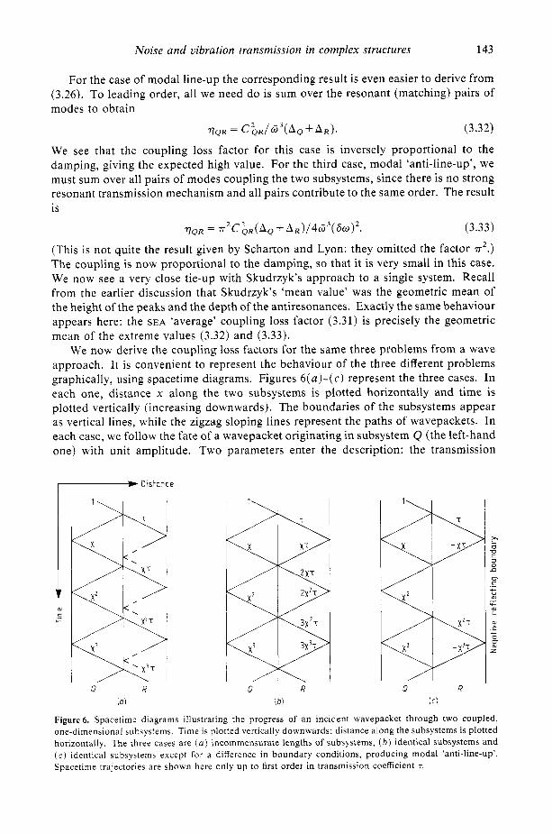
Noise and vibration transmission in complex structures 143
For the case of modal line-up the corresponding result is even easier to derive from (3.26). To leading order, all we need do is sum over the resonant (matching) pairs of modes to obtain
V Q R = C ; R / ~ ~ ( A Q + A R ) . (3.32)
We see that the coupling loss factor for this case is inversely proportional to the damping, giving the expected high value. For the third case, modal ‘anti-line-up’, we must sum over all pairs of modes coupling the two subsystems, since there is no strong resonant transmission mechanism and all pairs contribute to the same order. The result is
~ ) Q R = T’C&(AQ + A ~ ) / 4 6 ~ ( 8 W ) * . (3.33)
(This is not quite the result given by Scharton and Lyon: they omitted the factor T’.) The coupling is now proportional to the damping, so that it is very small in this case. We now see a very close tie-up with Skudrzyk’s approach to a single system. Recall from the earlier discussion that Skudrzyk’s ‘mean value’ was the geometric mean of the height of the peaks and the depth of the antiresonances. Exactly the same behaviour appears here: the SEA ‘average’ coupling loss factor (3.31) is precisely the geometric mean of the extreme values (3.32) and (3.33).
We now derive the coupling loss factors for the same three problems from a wave approach. It is convenient to represent the behaviour of the three different problems graphically, using spacetime diagrams. Figures 6( a ) - ( c) represent the three cases. In each one, distance x along the two subsystems is plotted horizontally and time is plotted vertically (increasing downwards). The boundaries of the subsystems appear as vertical lines, while the zigzag sloping lines represent the paths of wavepackets. In each case, we follow the fate of a wavepacket originating in subsystem Q (the left-hand one) with unit amplitude. Two parameters enter the description: the transmission
>.
0 V
3 0 .D
m c c U m
U. m i
m > c 0
z
-
-
m
Figure 6 . Spacetime diagrams illustrating the progress of an incident wavepacket through two coupled, one-dimensional subsystems, Time is plotted vertically downwards; distance along the subsystems is plotted horizontally. The three cases are ( a ) incommensurate lengths of subsystems, ( b ) identical subsystems and ( c ) identical subsystems except for a difference in boundary conditions, producing modal ‘anti-line-up’. Spacetime trajectories are shown here only up to first order in transmission coefficient T.

144 C H Hodges and J Woodhouse
coefficient 7 (assumed small, so that the reflection coefficient is taken as unity for the purposes of this leading-order discussion) and the amplitude attenuation factor x for a round trip in subsystem Q. Recall that from the discussion of 0 2.2, this latter quantity satisfies
x2 = exp (-27rA/Sw) (3.34)
where 60 is the frequency spacing for subsystem Q and A is a typical modal damping factor. In terms of these two quantities, the amplitudes of the travelling wavepackets are labelled at various stages on their journeys, using the simplifying assumption that damping is the same in both systems.
Figure 6(a) illustrates the case where the lengths of the two subsystems are incommensurate. This corresponds to statistical independence of blocked-mode frequencies in the two systems. On each reflection of the wavepacket in system Q from the coupling point, a fraction 7 leads through into system R. This then reflects back and forth there, and to leading order in T all its energy is dissipated there: no coherent interactions ever take place at the coupling point with the packet reflecting in system Q, since they never arrive at the same moment. Now for all these weak- coupling problems, the coupling loss factor TQR is simply the fractional energy loss per radian through the coupling. Thus for this case it is given by
TQR = I TI26W/ 2 ?TG (3.35)
where S o here is the frequency spacing in the source subsystem Q (as is necessary to satisfy the reciprocal relation (3.2)). Note that (3.35) is simply the coupling loss factor from Q to a semi-inJinite system R, since no effects of the length of R have entered the argument. This treatment of coupling loss is thus analogous to the earlier discussion of power input (0 2.2), where the infinitely extended system could be used in a similar way. When the transmission coefficient 7 is expressed in terms of our mode-coupling parameter CQR, (3.35) agrees with the Scharton and Lyon result, (3.31). The identity of these two results is the analogue of the Fermi ‘golden rule’ in quantum mechanics, which governs the transition rate from an initial quantum state Q to a final state R (Born 1957, Bohm 1960).
To discuss the case of modal line-up, we consider systems Q and R to be identical. The situation is then as illustrated in figure 6(6). This time, we have constructive interference effects occurring at the coupling point, so that the proportion of the input power eventually dissipated in system R and thus the energy flow, is increased. We can calculate the coupling loss factor by the same argument as before, and after summing the appropriate series we find
(3.36)
But for small damping, the factor
1+x2 so --_ l -X2- . i rA
in the notation of (3.31)-(3.33), so again the result is in agreement with the modal analysis. It also agrees with the result given by Smith (1980) in the small-.r approxi- mation.
The final case, modal anti-line-up, is slightly less obvious from a wave viewpoint. We can achieve the condition on mode frequencies by imposing different boundary

Noise and vibration transmission in complex structures 145
conditions at the extreme ends of the two systems Q and R while keeping the lengths of the two systems equal. Thus we have indicated in figure 6 ( c ) a negative-reflecting boundary in system R. Now instead of constructive interference at the coupling point, we have destructive interference. At every alternate round trip, the wavepackets in subsystem R cancel exactly. Some energy is still dissipated there, but the amount is drastically reduced by this cancellation. Performing the same calculation for the coupling loss factor, we obtain this time
(3.37)
The geometric-mean relation between the three cases (3.35)-(3.37) is particularly clearly displayed here.
These calculations shed some interesting light on the question of the extent to which a wave approach can be used for a general discussion of the validity of SEA,
similar to the mode-coupling discussion which we have given in previous subsections. There, we were able to list several assumptions made in the conventional justification of SEA which could be discussed to an extent separately: equipartition, modal incoher- ence, and so on. It seems natural to enquire after a similar set of assumptions in wave terms, but we shall find that the possibilities are very limited.
Another remark by Smith (1980) is at first sight suggestive in this context: for the kind of problem we have just discussed, with two coupled one-dimensional systems (which may form part of a larger system), he showed that a very simple form of the SEA energy-flow relation follows from an assumption of incoherence between the wave trains incident on the coupling from the two sides. His analysis assumes (as indeeed has ours above) that if the systems have evanescent solutions (e.g. near-fields on bending beams), there are no evanescent fields originating elsewhere in the structure with significant amplitude at the coupling (though the outgoing fields at the coupling are of course included in the calculation of reflection and transmission coefficients). Using the argument we have given in. 4 2.3 to relate wave fluxes to modal energies, it is easy to show that the total flow between the subsystems obeys
(3.38)
in terms of the energy reflection and transmission coefficients R and T (=1712) and the excitation bandwidth B. For a non-dissipative coupling we would have R + T = 1, but we have not assumed this here. Equation (3.38) is the SEA proportionality law, and for the case of weak coupling it gives the same coupling loss factor as (3.35) above.
Smith’s result suggests that incoherence of incident wave trains might play a similar role to modal incoherence in establishing the scope of validity of a SEA model. However, the relation between the two is rather complicated, as is illustrated by the calculations above of the coupling loss factors (3.35)-(3.37). For the one-dimensional systems considered here, it is fairly easy to see that the modal coherence induced by the coupling is determined by coherences of wave trains on either side of the coupling, but we must include the outgoing as well as incoming waves. The outgoing waves are always coherent to an extent, of course, since they have a common origin: this contribution to the modal coherence is responsible for the usual SEA estimate exemp- lified by (3.35). If the incoming waves are also coherent, we have seen in the cases of modal line-up and anti-line-up that the coupling loss factor may be very different, but

146 C H Hodges and J Woodhouse
in both of these cases the SEA proportionality law still holds since we are dealing with weak coupling. In this respect an assumption of incoherence of incoming wave trains is rather unhelpfully restrictive here.
Indeed, as Smith (1980) recognised, for one-dimensional systems like these, incom- ing wave trains are never entirely incoherent provided the system is reverberant. When we allow for effects to the next order in the transmission coefficient, omitted in figure 6, we include the round-trip paths through the whole system illustrated by a spacetime diagram in figure 7 . The pair of paths illustrated here will produce a measure of coherence between the incoming waves at the coupling under all circumstances, even for the case of rain-on-the-roof driving over the whole system, which produces modal incoherence and leads to the thermal equilibrium result. The energy fluxes will balance in this case, of course, since the thermal equilibrium result is still true, but the wave trains will not be incoherent.
Only when we go to subsystems with higher dimensionality does the assumption of wave train incoherence come into its own. In room acoustics, for example, it is a consequence of the diffuse field assumption described in 5 2.3. In that case, it may well be a good approximation for rooms with boundaries of complicated shape, containing scatterers of all length scales; see for example the discussion by Cremer er a1 (1982). A wave analysis of higher-dimensional systems is far more complicated than the one-dimensional cases we have discussed here, because the directional depen- dence of the transmission and reflection properties of the boundary must be taken into account, as well as the far harder multiple scattering behaviour within the subsystems and we attempt no discussion here. (Of course, a detailed modal analysis of such problems is also very complicated!)
Distance 7
x \I ,
Q R
Figure 7. Spacetime diagram similar to figure 6 , illustrating higher-order wavetrain coherences occurring in incommensurate subsystems.

Noise and vibration transmission in complex structures 147
Perhaps the nub of the problem of a wave approach to general issues of the validity of SEA is that there is no equivalent of the stochastic equations: no general way of casting a wave problem into energy variables alone. Only in certain regimes can this be done, and then the wave approach returns to prominence. Classical transport theory using the Boltzmann diffusion equation approach is one example and this is appropriate in precisely the same limit as geometric room acoustics mentioned earlier. Another example is the approach to transmission through random media using the forward- scattering approximation (Uscinski 1977). Here, it is possible to formulate equations for the propagation not only of the field intensity but also of higher moments of the field amplitude.
To sum up, we have a rather curious picture of the usefulness of the wave approach. We have seen in § 2 that it is quite powerful in the analysis of the behaviour of a single system. We have now seen that it is surprisingly unhelpful for general problems involving coupled systems, although it can be extremely useful for specific problems. From the point of view of SEA, it suffers from a similar drawback to that mentioned earlier (§ 3.4) for the admittance matrix method: to use either approach, one first solves the problem of how the coupled system responds to driving, then retrospectively asks whether SEA could have been used! In §§ 4.3 and 5 , we shall see that a wave approach comes back into its own in the context of localisation, which raises some more subtle problems than we have so far discussed. For some of these problems, a multiple scattering wave analysis is very useful.
We end this section with an aside relating to (3.38). In this sort of treatment of power transmission it is sometimes implicitly assumed that the forward and backward travelling fluxes in each subsystem are equal in magnitude so that the net intensities are just obtained by doubling the incident intensities. Smith (1980) calls this the symmetric jield approximation. It amounts to setting 1 + R - T = 2 in (3.38) and is clearly valid in the weak-coupling limit when the reflected intensity tends to unity. The symmetric field approximation is less good when the transmission approaches unity for strong coupling. This is because it does not predict the difference in modal energies correctly (since for weak reflection they are almost equal), not because the field is substantially asymmetric! It is interesting to note that (3.38) is also relevant to a closely related problem in a different field. In the theory of electrical conduction in disordered solids the electrical resistance of a one-dimensional aperiodic potential is well known to contain a factor (1 + R - T ) / T ( = 2 R / T ) , where T is the transmission probability through the potential and R = 1 - T because no electrons are lost during transmission (Landauer 1970).
4. Energy transmission in random media
The subject of this section can be regarded as the continuous analogue of the problem discussed in the previous section. We shall be considering wave transmission through continuously disordered random media, for example a turbulent fluid, and also through continuous structures with inhomogeneities placed either periodically or irregularly. We shall be particularly concerned with systems obtained by some kind of disordering of a periodic structure-for example, those obtained by varying the orientation or spacing of nominally parallel periodic ribs on a plate. Of course, the latter sort of structure is not continuously disordered and one could also think of treating it as a discrete set of coupled subsystems using SEA. We shall return to this idea in § 5 , but

148 C H Hodges and J Woodhouse
here we shall study these structures within the context of theories which also apply to the continuous case.
We must distinguish at the outset between local and extended disorder. By extended disorder we mean random deviations from uniformity or precise periodicity which extend uniformly (in a statistical sense) throughout a large structure. By local disorder we mean structural irregularity which occurs in a limited region of a periodic structure. Typical examples of the latter are a point defect in the atomic lattice of a solid or a junction of sections of different periodicity (such as the interface between two solids). The effect of local disorder has been much studied in solid-state physics in connection with the vibrational properties of lattice defects (Elliott 1966, Wallis 1968, Maradudin and Nardelli 1969). It is not difficult to think of structures of engineering relevance which correspond to these examples of imperfect crystal structure and some of these have been discussed in the literature (e.g. Cremer et al 1973, Mead and Lee 1984).
In this section, however, we shall mostly be concerned with the case of extended disorder, which raises some rather intriguing and subtle questions, some of which are of wider relevance to the use of statistical methods in acoustics and to SEA in particular. The material to be discussed falls broadly under the heading of ‘wave propagation in random media’. For the present purpose the distinction between a continuously disordered random medium and a disordered periodic structure is not a very important one from a theoretical point of view; the deviations from periodicity we shall be considering scatter the Bloch waves (see below in 5 4.1) of the underlying periodic structure in much the same way that inhomogeneities scatter waves in a continuous random medium and the same sorts of theoretical procedures are applicable in both cases. The wide variety of theories and techniques used in this general area has more to do with coping with different regimes of the physical parameters and also with the different kinds of information one may require.
We can cite two simple examples of particular regimes requiring their own appropri- ate theories. The first is the regime where scattering is primarily in the near-forward direction. This is often the case for electromagnetic wave propagation or in underwater acoustics, where the spatial extent of inhomogeneities (for example, fluctuations in salinity or refractive index) is large compared to the wavelength. In this regime one may replace the exact wave equation by the forward-scattering ‘parabolic’ approxima- tion, which substantially simplifies the treatment of multiple scattering (Uscinski 1977, 1982). In structural vibration, on the other hand, inhomogeneities such as ribs on a plate are frequently small compared to the wavelengths of interest and back-scattering is in general important, leading to theories of the kind to be discussed in this section, in which different approximations are made. Theories based on the forward-scattering approximation are of rather peripheral interest to this review and we shall not discuss them in detail.
An important general feature distinguishing different theories concerns the type of statistical information they provide. In principle, one would like to be able to calculate the statistical distribution of any physical quantity one is interested in. In practice, one often has to make do with averages over an ensemble of realisations of the random medium. The theories one uses will depend on the quantity one wishes to average. For example there exist theories describing the propagation of the ‘coherent wave’, the average of the wave field, which excludes the random fluctuations in the wave induced by scattering. If, on the other hand, one is interested in the propagation of wave energy, including the incoherent contribution, one may have to deal instead with averages of the wave intensity (Howe 1973). Averages of even higher powers of the

Noise and vibration transmission in complex structures 149
wave amplitude are of interest in some problems, for example in calculating the ‘scintillation index’, which quantifies the twinkling of stars due to disturbances in the atmosphere (Uscinski 1977, 1982, Uscinski et al 1983).
The distinction between averages of the wave and of the wave intensity is crucial when we discuss the question of localisation, which we have already described briefly in the introduction. The coherent response of a random medium is always localised in the region of the source, because it loses energy to the incoherent wave which continues to propagate outside this region (Howe 1973). The phenomenon of Anderson localisation concerns the possibility of the eventual localisation of the incoherent wave (over a larger region).
The technique of ensemble averaging is not without pitfalls even when an appropri- ate choice of physical quantity for averaging has been made. It can happen that the average is weighted by a few anomalous values which are very much larger than the ‘typical’ values one is interested in. We shall see an important illustration of this point in connection with the theory of Anderson localisation. When such behaviour occurs, in order to understand the behaviour of a typical member of the ensemble one needs to find out more about the statistical distribution than just its mean value.
In the next subsection we deal briefly with propagation in periodic structures in order to set the stage for the discussion of random media. It is also convenient to include there a very brief discussion of theories of the coherent wave in disordered systems. All these theories aim to replace the disordered system with an equivalent periodic structure which includes some of the effects of scattering by the deviations from periodicity-this is indicated by the name of the simplest such approach, the ‘quasi-crystalline approximation’ (Lax 1952).
In the remainder of this section we discuss theories which address the problem of incoherent wave-energy transport in disordered systems. For this purpose one would like a method of recasting the wave equation into energy variables as was done in 0 3.4 for the stochastic equations. As noted above, this cannot be done in general except in a perturbative scheme which requires some form of weak coupling assumption. This is what makes the general treatment of wave-energy transport potentially very difficult. In § 4.2 we discuss diffusive transport theory, the continuous analogue of SEA, and in 9 4.3 we discuss, at rather greater length, the phenomenon of Anderson localisation.
4.1. Periodic structures and coherent wave theories
We now briefly review the theory of wave propagation in periodic structures and some of the applications of this theory to structural vibration (for a recent review article on this subject see Sen Gupta (1980)). The determination of wave propagation in periodic structures is enormously simplified as a result of the Bloch (or Floquet) theorem which relates the wave solutions in adjacent bays of the system (Brillouin 1946, Ziman 1964). As an example, we consider a periodically restrained bending beam (Mead 1970), illustrated in figure 8. If the beam is infinite in extent, pairs of solutions can be found with time-harmonic variation exp ( iwt ) such that the spatial variation of the transverse beam velocity satisfies
V(x+ n d ) = exp ( inkd) V(x) (4.1)
where d is the restraint spacing and k is the Bloch wavenumber. Either this wavenumber is pure real, in which case V describes a travelling wave on the infinite beam, or it

150 C H Hodges and J Woodhouse
Figure 8. A periodically restrained bending beam, vibrating in the lowest pass band with a Bloch period of four bays. Notation for restraint forces and positions is also shown.
can have an imaginary component, in which case the solutions are of near-field or evanescent character, one growing and one decaying along the beam. For each solution the functional relation between the Bloch wavenumber k and frequency w defines the dispersion curve for that particular wave type. If for a given frequency there are no travelling-wave solutions, that frequency lies in a stop band, otherwise it lies in a pass band. The normal modes satisfying the boundary conditions on a periodic system of finite extent are appropriate combinations of the Bloch (or Floquet) functions defined above, the usual case being a superposition of a forward and a backward travelling wave together with near-field components at the ends to form a standing wave with approximately an integral number of half-wavelengths fitted into the length.
The same principles apply to systems showing periodicity along two or more directions, for example grillages (Heck1 1964) or plates having crossed-beam stiffening (Mead and Parthan 1979). In this case translation through n , periodic elements in direction 1 and n2 periodic elements in direction 2 multiplies the Bloch function by a factor exp [*i(n,k,d, + n2k2d2)]; the Bloch wavenumber has now become a vector with components k, and k,. However, we do not discuss such higher-dimensional periodicity in detail.
Another important case of symmetry along two directions is that of regularly spaced parallel ribs on a flat plate. This has continuous translation symmetry (as opposed to the discrete translation symmetry associated with periodicity) parallel to the ribs. Here, the spatial variation parallel to the ribs can be chosen to be pure harmonic and factored out, leaving a problem analogous to the periodically restrained bending beam for each harmonic component separately. These harmonic components represent independent channels for transmission of wave energy perpendicular to the array of ribs.
The free wave propagation in such systems can be determined by a variety of methods similar to those used in the study of electrons in crystals (Callaway 1964). We summarise here three of the most useful of these methods. The acoustical problem is in some ways more straightforward than the quantum mechanical one: for example, one can use an expansion of the Bloch function V(x) in plane waves without having to worry about orthogonalisation to core electrons (Ziman 1964, Harrison 1970).
This leads to the first of the approaches which we describe: the travelling-wave Bloch function for a system showing one-dimensional periodicity (such as the restrained bending beam) can be written (Mead 1970, Mead and Pujara 1971) as
(4.2) ) V(X) = exp (ikx) 1 c, exp (f.irinx/d)
which is equivalent to (4.1). Rayleigh's principle is then applied, with a truncated set of the coefficients c, as variational parameters. Particularly for bending vibrations of beams or plates (where bending stiffness eliminates any kinks) the Fourier series (4.2)
L

Noise and vibration transmission in complex structures 151
converges rapidly and errors arising from its truncation do not pose major problems. This method has recently been applied with considerable success to a detailed study of the low-frequency behaviour of a circumferentially stiffened cylinder, a structure of some practical importance (Hodges et a1 1985a, b).
The second type of method we describe avoids any truncation problems and is applicable to systems showing periodicity in one dimension. It uses the representation of the Bloch function within each bay of the structure as a superposition of free waves of the unconstrained beam, plate, etc. Thus, as an example, in the nth bay of the periodically restrained beam one writes
V(x,)=exp (inkd)[A exp (iKx,)+B exp (-iKx,)+C exp (KX,,)+D exp (-KX,)]
(4.3)
where x, = x - n d and K is related to frequency w by the dispersion relation of a uniform beam. The dispersion relation between k and w for the restrained beam is obtained by imposing continuity of V and its derivative V' across the restraints, and discontinuities in V and V related to the rotational and displacement impedances of these restraints. This calculation has been worked out in detail for the restrained- beam problem by Mead (1970) and the approach can be applied to other structures, for example ribbed cylinders (Avallet and Parot 1982).
At higher frequencies such that exp (-Kd) is small, the near-field components corresponding to the last two terms in (4.3) are localised close to the restraints and do not contribute to the multiple scattering of waves in the structure. (This is an approximation we have used in the previous section.) Under these conditions the Bloch wavenumber is particularly easy to determine; it depends only on the transmission coefficient t of an isolated constraint (Heck1 1964, Cremer et a1 1973), so that
cos kd = Re [ t-' exp ( i ~ d ) ] . (4.4)
Finally, we discuss another powerful approach, known as the 'KKR Green function method' in the context of electrons in crystals (Ziman 1964, Callaway 1964). We illustrate it here for a bending beam on which the restraints exert forces FJ at positions xi (see figure 8). For simplicity, the rotational impedance of the restraints will be neglected. The response of the beam at restraint i is given by
V ( X ~ ) = 1 G(x, - x,, w ) F , i
(4.5)
where G(x, -xJ, w ) is the transfer admittance of the unconstrained beam, which we assume to be known. But V(x,) is also the velocity of the ith restraints, and so can be expressed in terms of Z,(w), the impedance of that restraint. Thus
C G(x,-x,,w)F,+Z;'F,=O. (4.6) J
This equation is not limited to the case of a periodic system-the free wave propagation problem is solved quite generally by looking for the zeros of the determinant of the matrix
M,,=G(x,-x,, w)+Z;'6,,. (4.7)
To apply (4.6) to the periodic case, we set xJ = jd, Z , ( w ) = Z ( w ) and impose the Bloch variation from (4.1) for the forces 5. Such an approach has, for example, proved

152 C H Hodges and J Woodhouse
useful in problems involving fluid-loaded plates with periodic stiffeners (Romanov 1971, Evseev 1973, Kovinskaya and Nikiforov 1973, Rumerman 1975, Mace 1980a, b, Eatwell and Butler 1982, Crighton 1984).
We end this subsection with a brief discussion of theories treating the coherentjeld in a random medium or structure with extended disorder. It is convenient to distinguish between systems where there is some obvious associated periodic structure and those where there is not. Examples of the former include engineering structures which are nominally periodic but have small deviations from the ideal design or, at the atomic level, a substitutional alloy. Examples of the latter are gas bubbles in a liquid or the atomic structure of a liquid. The latter cases are more difficult to treat theoretically, particularly for extreme ranges of the physical parameters corresponding to strong and concentrated scatterers. Thus there is a simple and successful theory treating the substitutional alloy, the so-called ‘coherent potential approximation’ (Soven 1967, Taylor 1967, Ziman 1979), but there is no simple equivalent theory for the electronic structure of a liquid or for phonons in a topologically disordered solid (Ziman 1979). A number of acoustical applications come under the second heading above-for example, sound propagation in porous or composite materials (Attenborough 1982, Willis 1981) and through gas bubbles in a liquid (e.g. Foldy 1945, Waterman and True11 1961) and boundary waves trapped near a rough surface (Tolstoy 1983). The corre- sponding theories are less relevant to the subject matter of this review and will not be discussed here.
Eatwell (1983) has given a good illustration of the coherent wave approach applied to a disordered structure coming under the first heading above. He uses the quasi- crystalline assumption of Lax (1952) to derive a dispersion relation for the coherent component of the free wave on an irregularly stiffened fluid-loaded plate. This assump- tion means that we characterise the propagation by a frequency-dependent Bloch wavenumber, as if it were a periodic structure. The effect of irregularity is to give this wavenumber some imaginary component describing the spatial decay of the coherent wave due to scattering into the incoherent component. This occurs at all frequencies, including those lying within the pass bands of the underlying periodic structure. Eatwell’s work appears to be the only investigation of coherent wave propagation described in the literature of structural vibration, and we shall not go into this subject in any further detail.
4.2. Kinetic theory
We now discuss an approach to multiple scattering in a random medium or a disordered structure, which includes a description of the incoherent wave intensity. On a long enough timescale the propagation of the incoherent wave intensity proceeds by way of diffusion. Theories of this diffusion process come under the general heading of transport or radiative transfer theory (Ishimaru 1978, Chandrasekhar 1960) or kinetic theory (Howe 1972,1973). Kinetic theory is so called because it describes the propaga- tion and scattering of wave energy in the form of wavepackets which correspond to particles and may therefore be treated by the methods of classical kinetic theory (e.g. Mayer and Mayer 1977). This suggests some kind of short-wavelength restriction: certainly these theories require a wavelength short compared with the mean free path for scattering but they do not require short wavelength compared with the size of scatterers. However, to understand the precise conditions under which kinetic theory is a valid approximation is by no means straightforward, as we shall see.

Noise and vibration transmission in complex structures 153
In the theories to be described here, the general law governing wave-energy transport in a disordered system has the form
l I = - D V I (4.8)
where lI is the energy current density and D is the diffusion coefficient. This expression is the natural analogue for applications to homogeneously disordered systems of the SEA energy-flow proportionality relation. As we saw earlier, the energy density I is related to the modal energy by (2.18). Since there are no discrete boundaries the difference in modal energies between subsystems is replaced by its continuous analogue, the gradient of the wave-energy density. There is evidently a very close connection between SEA and transport theory in disordered systems.
Kinetic theory is to some extent the wave-scattering counterpart of the mode- coupling approach to SEA described in § 3. Here we start with propagating waves which are coupled by scattering from the inhomogeneities and we derive a Boltzmann equation expressed in energy variables which plays a similar role to the weak-coupling results in our earlier discussion of SEA. Strictly speaking, D applies to the diffusion of wave energy at a particular frequency. If we are treating diffusion of wave energy within a frequency range where D is roughly constant, (4.8) together with conservation of energy leads to the diffusion equation
DV21 = a I / a t -k A I (4.9)
for propagation of energy density. Here we have included a term which describes absorption of energy by the medium with a damping coefficient A(x), where x is the position vector.
The scattering processes determine the diffusion rate: in terms of the mean free path for back-scattering I, the diffusion constant D is given by
D = $cg1 (4.10)
where cg is the group velocity at the frequency in question (Feynmann et al 1963). The simplest and most commonly used method of calculating the mean free path is via the Born approximation for local scattering (Ziman 1964, Howe 1973), which requires scatterers to be weak in some sense. However, the validity of the Born approximation in describing the local scattering process is neither necessary nor sufficient for the validity of a diffusive model for the global behaviour. Detailed derivations of the Boltzmann equation for wave-energy transport are given in many textbooks, for example those on solid-state physics such as by Ziman (1964), and have been discussed in an acoustical context by Howe (1972, 1973). As we have already indicated, the justification of the method is by no means simple; while the local scattering may be weak, its global effects can still be strong and there is no obvious rationale for neglect of higher-order corrections.
Essentially, kinetic theory treats multiple scattering between inhomogeneities but does not attempt to keep track of the phase of waves between scattering events because it is formulated solely in terms of energy variables. As we shall see in our discussion of the theory of Anderson localisation, allowing for phase information in the description of multiple scattering can have very dramatic consequences in some situations, par- ticularly in one-dimensional systems. On the other hand, for weak scattering in systems of higher dimensionality diffusion theory works perfectly well. Another situation in which kinetic theory works well is when the scatterers are time-varying: the subtle phase coherences between back-scattered waves which give rise to localisation tend

154 C H Hodges and J Woodhouse
to be destroyed. Kinetic theory can, in fact, be regarded as a limiting case of a more general theory to be discussed in the next section, which includes a description of the phenomenon of Anderson localisation as well. We shall return to this discussion of the conditions under which kinetic theory is valid in 0 5.
A more fundamental approach to transport theory is based on a ‘diagrammatic’ expansion of the ensemble-averaged wave-intensity propagation function (+(x’, t ’ ) *+(x , - t ) ’ ) (Edwards 1958, Frisch 1967, Rybak 1972, Ziman 1979). Kinetic theory is equivalent to solving the Bethe-Salpeter equation for this quantity in the ladder approximation (Salpeter and Bethe 1951). This approach has been used by Rybak (1972) to discuss the propagation of long waves along a randomly inhomogeneous flexible beam. The advantage of the diagrammatic approach is that one can investigate corrections to the local Born approximation by going beyond the ladder approximation (Langer and Neal 1966), in a way somewhat analogous to our use of the stochastic equations in 0 3.4 (but requiring an infinite number of corrections beyond the Born approximation). This is one possible approach to the phenomenon of Anderson localisation (e.g. Abrahams et a1 1979, Wolfle and Vollhardt 1980) but not one we shall describe.
Equations (4.8) and (4.9) are of relevance to studying diffusive propagation of acoustical energy in a variety of situations. Some of these do not involve structural vibration but nevertheless fall within the scope of this review from a conceptual point of view. For example, sound propagation through vegetation and between buildings has been investigated using kinetic theory (Bullen and Fricke 1982, Bullen 1983, Kuttruff 1982). An amusing application of this approach concerns the question of the reverberation following a pistol shot in a forest (Kuttruff 1967). If absorption is neglected, the diffusion equation predicts an eventual decay in energy density I proportional to tCd’* after time t, where d is the dimensionality. If no sound escaped through the tops of the trees the relevant dimensionality would eventually be d = 2. Hardly surprisingly, measurements of the decay rate do not agree precisely with this prediction (Kuttruff 1967) ! Other applications of kinetic theory to acoustics include scattering of sound by turbulence (Howe 1973) and wave propagation in flexible plates and beams (Howe 1972, Rybak 1972, Nikiforov 1980).
A recent application of kinetic theory concerns sound propagation in cylindrical ducts lined with material which absorbs and scatters energy propagating in the various waveguide modes (Howe 1983). The question arises as to what sort of liner will give the maximum attenuation. If the liner properties vary both axially and circumferentially as they do for a ‘checkerboard’ liner, the energy can scatter into modes travelling slowly (because they are close to a waveguide cut-off), for which the spatial attenuation due to dissipation in the liner is rapid (Smith 1981, 1982). Howe used kinetic theory to determine the overall attenuation for a checkerboard liner whose properties vary randomly over the surface of the duct. For this application, kinetic theory is expressed as a set of coupled one-dimensional differential equations governing the variation of acoustic energy in each waveguide mode along the duct.
4.3. Localisation
To get any further in understanding when kinetic theory is valid, we need to know in what ways it can break down. This leads us to consider Anderson localisation. As a starting point for our discussion, we consider the effect of local disorder on the vibrations of an otherwise periodic lattice. The normal-mode frequencies for such a system may

Noise and vibration transmission in complex structures 155
be obtained straightforwardly in principle by solving a matrix equation of finite order whose elements are expressed in terms of the transfer function of the periodic lattice (Elliott 1966, Wallis 1968, Maradudin and Nardelli 1969). Although we shall not discuss studies of local disorder in detail here, one idea of considerable importance does emerge from such investigations. For periodic lattices with local defects it is possible for a small fraction of the normal-mode frequencies to lie in a stop band of the periodic structure and the corresponding modes will then be localised in the region of the defect. This becomes clear if we consider the structure as two systems, each driving the other, one of them containing the defect. For mode frequencies in a stop band the mode amplitude must decay exponentially away from the defect, since the response of the lattice to driving by the defect region is purely ‘near-field’ at these frequencies. By the same token, modes with frequencies in the pass band must be extended throughout the structure.
The phenomenon of Anderson localisation, which occurs in systems with extended disorder, is related to the behaviour of lattices with local defects, but with some important differences and added subtleties. As the simplest illustration consider a chain of pendula coupled together by springs, with random fluctuations from pendulum to pendulum in frequency. (Such a chain was illustrated in figure 4.) One would not be too surprised to find localised modes whose frequencies lie in what, before disorder- ing, was a stop band of the periodic system. After all, there must exist regions which look somewhat like local defects, consisting, say, of an exceptionally high-frequency pendulum surrounded by others whose frequencies are close to the average. The remarkable fact, known from work on the analogous problem of an electron in a random potential, is that for this one-dimensional system all modes are localised, even for weak disorder (e.g. Mott and Twose 1961, Thouless 1973). This includes the modes whose frequencies lie within what was previously the pass band. In this frequency range localisation cannot be understood in terms of the near-field response of the underlying periodic structure; it is a more subtle effect arising from the cumulative effect on the mode shapes of disorder extended over large distances.
Central to this subject is the idea of a localisation length scale, which roughly speaking defines the size of region over which the amplitude of a particular localised mode is large. On a greater length scale the modal amplitude will decay exponentially (on the average) away from this region, though there will be considerable fluctuations in amplitude about the average decay envelope. A computed example of a localised mode in a simple one-dimensional system is shown in figure 9, taken from Borland (1963). Examples of localisation in the context of structural vibration are shown by measurements and computations of the modes of a mistuned bladed disc (Ewins 1973),
I
0 200 400 600 800 1000 Site number
Figure 9. Squared modal amplitude of a localised mode in a long one-dimensional disordered system, reproduced, by permission, from Borland (1963).

156 C H Hodges and J Woodhouse
and by measurements on a vibrating string with irregularly spaced added masses (Hodges and Woodhouse 1983). It is believed that the general characteristics of localisation behaviour (for example, the dependence of localisation length on an appropriate measure of disorder relative to coupling strength (Anderson 1958, Abrahams et a1 1979)) depend only on the dimensionality of the system and not on the particular model being investigated. This feature, which the localisation phenomenon is held to share with phase transitions in condensed matter, is known as ‘universality’ (Ziman 1979).
For weak disorder in one-dimensional systems localisation is weak, but as mentioned above exponential decay of the modes will always be seen on a large enough length scale. Most solid-state theorists believe the same to be true for disorder in two dimensions, though in this case the localisation length diverges much more rapidly as the disorder strength goes to zero (Abrahams et a1 1979). In three dimensions a finite threshold in the disorder strength must be exceeded in order to localise all the modes. For weaker disorder only modes near the edges of pass bands will be localised. (Were this not the case, there would be no normal metallic conductors of electricity!)
Localisation of modes implies localisation of the response to driving, which there- fore decays exponentially away from the driving point, on the average. This is evident from the expression for the response in terms of modal amplitudes, (2.4). Wave energy is confined to the vicinity of the source because it is totally reflected from the irregularities of the structure, which becomes as a whole non-transmitting. This confinement effect has been demonstrated experimentally for the vibrating string with irregularly spaced added masses mentioned above (Hodges and Woodhouse 1983).
The confinement effect due to Anderson localisation should not be confused with the attenuation of response due to energy absorption by damping. Localisation occurs even in the limit of vanishing damping and the exponential fall-off rate in this limit is unrelated to the damping constant. Damping can be of importance, however, in limiting the overall response; for broad-band excitation energy is injected continuously into the structure and cannot escape from the source region, so in the absence of damping the build-up of energy in this region would continue indefinitely. (The same is of course true of any closed system.) Confinement should also be clearly distinguished from attenuation of the coherent wave which, as we have discussed above, results from scattering into the incoherent component, which can continue to carry energy away from the source.
From the above discussion it is clear that Anderson localisation will be important when back-scattering is significant, in systems where the propagation is one-dimensional or possibly two-dimensional in character. This includes media which are layered in some way, for example rock strata (Levine and Willensen 1983) and, in structural acoustics, parallel stiffeners on a flat plate. The potential importance of the phenomenon in structural acoustics arises not only from the fact that many practical systems are, in fact, of low effective dimensionality but also because inhomogeneities like ribs can, depending on the angle of incidence, be strong reflectors. In fact, the possibility of decreasing vibration transmission across a series of parallel beams in practical applications by means of spacing and impedance variations has been proposed by Kirpichnikov and Kuz’michev (1977). In this and similar work (e.g. Lin 1976, Bansal 1978, 1980, Glushkov and Kuz’michev 1980) attention has focused on a numerical solution of the transmission across a relatively small number of beams or constraints. It has not generally been realised that this sort of problem is amenable to analytic treatment in the sense that typical values for, and indeed the statistical

Noise and vibration transmission in complex structures 157
distribution of, the transmission across an arbitrary number of constraints can be obtained without numerical computation under a variety of limiting conditions (Hodges 1982).
Much of the work in acoustics concerning wave propagation in random media is concerned with transmission through fluids and is applied to regimes where Anderson localisation does not occur. In particular, in underwater acoustics one is dealing with predominantly forward-scattering and three-dimensional (or at least two-dimensional) propagation. Even in this context, though, there has been some theoretical work bearing on localisation. Wenzel (1982, 1983a, b) has discussed the existence of an ‘excess attenuation’ in the mean intensity of waves propagating in a one-dimensional random medium. The excess attenuation occurs in addition to that due to absorption and is a result of back-scattering by random fluctuations. His excess attenuation rate is in quantitative agreement with the localisation length given by other workers (e.g. Thouless 1973, Scott 1985) for such a medium. However, in three-dimensional random media exponential localisation is not manifested unless the back-scatter is very strong- much stronger than it is in underwater acoustics. There may still be excess attenuation in some sense due to back-scatter but it should be possible to treat this by conventional transport theory (Ishimaru 1978), in other words by methods similar to those discussed in the previous subsection.
Reviews of the theory of Anderson localisation with applications to solid-state physics in mind have been given by Thouless (1974, 1980), Ziman (1979) and Erdos and Herndon (1982); see also the proceedings of a recent symposium (Nagaoka and Fukuyama 1982). The literature in the field is vast and much of it highly technical. It tends to be concerned with regimes which are of less potential interest to structural acousticians. Thus a solid-state physicist may be concerned with weak localisation extending over a very large number of atoms or imperfections, of the order of Avogadro’s number. An acoustician will only be interested in the phenomenon if, for example, it manifests itself across the rather more limited number of ribs on his flat plate. We shall only review this literature to the extent that it sheds light on some of the acoustical problems we are concerned with here.
In view of the universality property mentioned above, one is at liberty to use the simplest and most convenient theoretical models to establish the general characteristics of localisation behaviour. Two types of model have been popular in the solid-state literature, both of which have acoustical analogues. In his original paper Anderson (1958) used a model which, in our terms, is equivalent to a set of coupled oscillators (or pendula) and is thus closely related to the mode-coupling approach to SEA. The oscillators are placed on a lattice, one to a site, and there is a constant coupling between nearest-neighbour sites, but the uncoupled oscillator frequencies vary randomly from site to site. The spread in these uncoupled frequencies gives a measure of the disorder strength. This is a suitable model for wave-bearing structures divided into bays which are weakly coupled by irregularly spaced constraints, for example a mass-loaded vibrating string (Hodges and Woodhouse 1983), and we shall return to it in 8 5. In terms of coupled oscillators the occurrence of localisation is more or less obvious if the coupling is sufficiently weak. The vibrations then approximate those for zero coupling, which are obviously ‘localised’ on individual oscillators or, for wave-bearing systems, in individual bays. From this point of view, it is the periodic system which is anomalous in its behaviour in this limit: the oscillators or the modes of adjacent bays have identical frequencies and are driving each other at resonance, so no matter how weak the coupling, if one waits long enough there can be complete interchange
158 C H Hodges and J Woodhouse
of energy between bays. The above plausibility argument for localisation in weakly coupled systems is given at greater length by Hodges (1982) and Hodges and Wood- house (1983). So far as it goes, it clearly applies to systems of any dimensionality.
People more used to thinking in wave terms might claim (incorrectly in fact) that this argument prejudges the issue since localised modes (the uncoupled oscillators or bays) are put into the model at the outset. Recent work has concentrated particularly on the critical case of localisation in two-dimensional systems, treated by the approach of scaling theory and the renormalisation group, and it has tended to formulate the problem in terms of multiple scattering of waves (Landauer 1970, Anderson et a1 1980, Anderson 1981, Erdos and Herndon 1982). A related approach has been used by Hodges (1982) to demonstrate the persistence of localisation for small constraint reflectivities of identical constraints spaced irregularly on a vibrating string or beam and we describe the simplest case of that analysis now.
We express the total transmission in terms of reflection and transmission of propa- gating waves at the constraints. Each constraint is defined to have a reflection coefficient r and a transmission coefficient t , where conservation of flux requires Irl2+ Itl2 = 1. For the bending beam case, we again make the assumption that the spacing between constraints is large enough for the near-field components not to affect the answer. The analysis is particularly simple if the variation in constraint spacing is larger than the wavelength on the string or beam so that the phase factors exp [iK(x,+l -xn)] are essentially random and uncorrelated, and this is the case we describe. Under these conditions it is readily shown (Anderson et a1 1980, Hodges 1982) that typical values of the total transmission across N constraints are of the order of
T N - t N (4.11)
and corresponding values of the transmitted intensity are of the order of
IN = ITN/2- ItlZN. (4.12)
We summarise the main points of the argument here. By associating a net reflection coefficient R, with the totality of constraints to the right of the nth constraint one can define a renormalised transmission coefficient t , at x, which is given by Cremer et a1 (1973); see also figure 4 of Hodges (1982):
(4.13) t , = t / ( 1 - rR,,).
In terms of t,, the total transmission is
(4.14)
The variation of the reflection coefficients R, is deduced from the recursion relations
Rn-' = exp [ 2 i ~ ( x , -X,-~)]RL-, (4.15)
RL-l = r + t2R,/(1 - rRn) . (4.16)
Boundary conditions are applied at the far end of the string by specifying RN When (4.15) and (4.16) are iterated towards n = O the phase of R, varies randomly with n for a typical solution because of the random phase factor in (4.15).
The example here provides a good illustration of the difference between typical values and ensemble averages alluded to earlier. Since typical values of the total transmission (4.14) are a product of randomly varying factors, the vast majority of values in the ensemble are given by the Nth power of the geometric mean. On the

Noise and vibration transmission in complex structures 159
other hand, the ensemble average is the Nth power of the arithmetic mean, which is by no means the same thing. If one is interested in the statistics the obvious procedure is to examine the distribution of the logarithm of the transmission since this is a sum of independent variables and will be Gaussian-distributed for large N. For an individual realisation we may take the logarithm of (4.14) and expand to obtain
N l n T N = N l n t - 1 ln(1-rR,)
n = O
m rP N
p = l P n=O = N l n t - 1 - 1 (R,)P (4.17)
(Since \rl < 1 the expansion is absolutely convergent, allowing the order of summation above to be interchanged.) For typical solutions R, has random phase and so the sum over n above is of the order of J N . We therefore have
In TN = N In t * O ( J N ) (4.18)
which gives our basic results in (4.11) and (4.12) to within a fluctuation factor exp (*dN) . If we ensemble-average (4.18), the fluctuation term would disappear. The typical decay is therefore given by the average over the ensemble of the logarithm of the transmission.
It is interesting to note that direct averaging of the transmitted intensity over the ensemble can give qualitatively different results. To show this we take the special case of a string or beam with zero dissipation and conservative boundary conditions at the far end; all magnitudes IR, I are then unity from energy flux considerations. The phase factors in (4.15) are random and uncorrelated in the ensemble, so that (Hodges 1982)
(4.19)
where p n is the phase of rR,, and the average ( ) here is over the p,. Localisation does not manifest itself at all in this case! Since the average over the ensemble is unity while the typical value is exponentially small, it is clear that the average is being dominated by a small proportion of members of the ensemble with very large trans- mission factors. (Note that conservative boundary conditions at the far end allow values of ITN)2> 1, which simply correspond to wave solutions which grow towards that end.)
The existence of occasional large transmission factors in this case can be understood by the following argument due to Borland (1963) and also discussed by Hodges (1982). The existence of some solutions with exponentially large transmission is implied by the reflection symmetry of the ensemble as a whole, since any decaying wave can be reflected to obtain another member of the ensemble with one which is growing. The asymmetry, i.e. the localisation effect, arises from the application of the boundary conditions at the far end. As Borland shows, waves which decay when (4.15) and (4.16) are iterated back from that end do exist, but the probability of encountering one is very small. The situation is similar to that in statistical mechanics where macroscopic irreversibility results from applying special initial conditions rather than from microscopic irreversibility of the equations of motion.
It should be stressed that more realistic examples with dissipation and radiative boundary conditions will show these statistical subtleties in a less dramatic way. For radiative boundary conditions there are no transmission coefficients greater than unity and the ensemble average will now show the localisation phenomenon, but still perhaps

160 C H Hodges and J Woodhouse
with a decay length greater than the typical value. Thus for transmission through a slab of one-dimensional random medium the ensemble decay rate as the sample length is increased is one quarter the typical value (Scott 1985).
We have gone through the analysis of this simple one-dimensional model in some detail, not only because it provides a simple demonstration of localisation which extends to weak scattering but also because it raises these important conceptual points concerning statistical averaging which are also of relevance to SEA theory, as will be seen in the next section. The analysis above applies to large variations in spacing relative to the wavelength. Small spacing variation can be similarly treated. (The treatment of localisation for irregularly spaced masses on a string given by Hodges and Woodhouse (1983) includes both large and small spacing variations.) The model can also be used as a basis for analysing more realistic situations of practical interest for noise and vibration control.
As an example we could consider a ribbed flat plate or cylinder. As mentioned in 04.1, the propagation can be decomposed into a series of channels, each of which corresponds to a different wavenumber parallel to the nominal rib direction, or on the cylinder to a waveguide mode with a particular angular variation. These channels may be decoupled or coupled depending on whether or not the translation symmetry along the ribs, or the cylindrical symmetry, is preserved. If the ribs are uniform and perpendicular to the cylinder axis, or parallel on the flat plate, then the channels are decoupled. (We have already met this argument in our discussion of acoustic propaga- tion in a lined cylindrical duct in § 4.2; peripheral segmentation or a checkerboard liner couples the channels but axial segmentation does not (Howe 1983).)
For parallel irregularly spaced ribs of similar properties the propagation in each decoupled channel can be described by the one-dimensional model analysed above provided the effects of near-fields are not significant. For ribs placed symmetrically on a plate the reflection and transmission coefficients t and r are given by Cremer et a1 (1973), who deal with the case of oblique incidence of a plane wave on an isolated rib. There always turns out to be at least one ‘coincidence angle’, for which the ribs become perfect transmitters because of trace wavenumber matching between rib and plate waves (see $3.5 and Ungar (1961)). The propagation in the corresponding channels will obviously be unaffected by irregularity. In order to limit vibration propagation one would need to use ribs of varying stiffness in order to vary the coincidence angle and to ensure reflection at some of the ribs in each channel (Cremer et a1 1973, Kirpichnikov and Kuz’michev 1977). (For the same reason, effective soundproofing by double glazing requires two different thicknesses of glass.)
In many cases of practical interest the translation symmetry parallel to the ribs will be broken, for example by welds on the structure, and the channels will therefore be coupled. The theory of localisation in the presence of channel coupling is much more difficult; indeed, it is precisely this problem which underlies much of the current debate on localisation behaviour in higher dimensions (Anderson 198 1). A detailed discussion is beyond the scope of this review but we shall touch on this topic again in 8 5 in connection with the relation between kinetic theory and localisation.
5. Implications of Anderson localisation for diffusive transport theories
5.1. Localisation and SEA
In this section we investigate the significance of localisation in determining the scope

Noise and vibration transmission in complex structures 161
of validity of the diffusive transport theories we have discussed earlier. In this subsec- tion, we consider the question of whether and when SEA can reproduce localisation behaviour: this will tie up some loose ends of the discussion started in 0 3. In 3 5.2 we ask whether some criterion for the validity of kinetic theory in continuously disordered random media can be given: we have seen in the previous section that for sufficiently high disorder in any number of dimensions, diffusion gives way to locali- sation.
Since localisation is a weak-coupling phenomenon, and since simple SEA (excluding the indirect coupling effects discussed in 00 3.3 and 3.4) is a weak-coupling theory, we should expect to find that SEA can incorporate some aspects of localisation. This will indeed turn out to be the case. However, the usual formulation of SEA for statistically independent multimodal subsystems outlined in 0 3.1 does not reproduce localisation, and we must start by understanding why not. The general form of a SEA model is given by (3.1), which we can rearrange to read
n R , l n = 1 XRQEQ (5.1) Q
where
xRQ [= - ~ N R ~ T R Q R + Q ( 5 . 2 )
= 2 ~ R s ( T R + c ?iRQ) R = Q. Q i f R
From such a model, the response pattern is found in terms of the driving by inverting the matrix XRo in (5.1). (This matrix is never singular provided all subsystems have non-zero damping, qR > 0.)
The question of whether a SEA model of this form gives a localised response to driving depends on the behaviour of the coupling loss factors as the dissipation, and hence the internal loss factors vR, tend to zero. When the coupling loss factor is calculated by the usual SEA procedure described earlier (assuming statistically indepen- dent mode frequencies), a typical result is given by (3.31): in particular, note that there is no dependence on the modal damping factors. Thus as the damping tends to zero, the coupling loss factors remain finite and non-zero. In the limit, the matrix XRQ in (5.1) becomes singular, which is not surprising for a closed system with no damping. As this limit is approached, the inverse of a matrix of the form (5 .2) ceases to depend on the values of the coupling loss factors and becomes uniform, leading to equipartition of the subsystem modal energies. The reason for this form of inverse is not hard to see. As the zero-damping limit is approached, the sum of elements in each row of the matrix tends to zero, so that there must be an eigenvalue tending to zero with an associated eigenvector having all entries equal. The standard expression for the inverse of a matrix in terms of its eigenvalues and eigenvectors will be dominated by the near-zero eigenvalue and hence by the dyadic product of this near-constant eigenvector.
However, if the coupling loss factors are proportional to the damping then the response can be localised. We can see this from the same matrix expression (5.1) and (5 .2) . In that case, a factor of A can be taken out of the whole matrix XRo Inverting this matrix then gives an overall response level proportional to A-' (since we still have a closed system) but with a distribution over the subsystems which tends to an invariant form as damping tends to zero. This invariant form will not in general be uniform over the subsystems. This is precisely the qualitative behaviour characterising Anderson localisation, which we explored in the previous section. Now, at the individual

162 C H Hodges and J Woodhouse
oscillator level the limiting values of the coupling loss factors are indeed proportional to the damping (except for accidental mode frequency degeneracy), as is seen from the factor in the numerator of the expression (3.23) for rrp (which gives the two- oscillator energy-flow proportionality constant by (3.26)). The usual result, indepen- dent of damping, arises by averaging over statistically independent mode frequencies within subsystems, producing a cancelling factor of damping in the denominator. Somehow, localisation has been lost in this averaging operation.
In discussing the absence of localised response in the usual formulation of SEA,
two related issues arise concerning this averaging process. The first issue concerns the validity of the assumption of modal equipartition. This assumption will be shown to break down for weak modal overlap, invalidating the averaging procedure usually used. In this limit it is necessary to average the response rather than the coupling loss factor. When this is done one recovers localisation, at least in qualitative form, as we shall see shortly.
The second issue to be discussed is the distinction between linear ensemble averages and typical values raised in § 4.3. The usual formulation aims primarily at a prediction of the linearly averaged response over an ensemble of realisations of the system or over a frequency band containing a large number of modes. The problem of estimating fluctuations about this value is recognised as being of considerable importance for narrow-band excitation but has received relatively little attention. The discussion of localisation in 5 4.3 shows that there are situations where these fluctuations become very large and where the linear ensemble average provides a very bad estimate of ‘typical’ values of the response.
To investigate the first issue we consider a set of weakly coupled subsystems, and we suppose that one of them is excited by rain-on-the roof driving, so that equipartition holds approximately in that system and all forces driving blocked modes are incoherent (see 5 2.2). Our main concern will be the extent to which equipartition holds in those subsystems which are not directly driven and the effect of any deviations from equiparti- tion on the energy flow. It will be shown that for multimodal subsystems with statistically independent blocked-mode frequencies the usual formulation of SEA sub- stantially overestimates the subsystem coupling loss factor for weak modal overlap in the driven subsystem.
The reasons for this overestimate are easy to see in qualitative terms. The usual formulation outlined in 5 3.1 averages the mode-mode coupling factor a,, given by (3.26) over modes r and q in the excitation band to obtain the subsystem coupling loss factor. This assumes modal equipartition within the subsystems, or at least that the modal energy difference E, - E, is uncorrelated with arq This assumption is, in fact, only valid for strong overlap, as we shall see. For weak modal overlap the average is strongly weighted by a small fraction of mode pairs whose blocked frequencies are near-degenerate and for which arq is inversely proportional to the damping as in the mode line-up result, (3.32). Since this fraction is proportional to the damping the resulting ‘statistical’ coupling loss factor, (3.31), is independent of damping. However it is clear that, under these circumstances, the modal energy difference cannot be uncorrelated with a,,. The effect of occasional large values of the latter is to reduce the corresponding values of the former rather than to contribute strongly to the energy flow. The problem here is equivalent to a series of bodies linked by heat conductors, a few of which are very good ones; these good conductors simply maintain equal temperature between their ends and the heat flow along them is determined by the other less efficient links in the system.
Noise and vibration transmission in complex structures 163
These points are borne out by examining a special case in more detail. Consider a subsystem Q which is not driven directly and which is taken to be coupled to one other subsystem R, all of whose blocked modes have kinetic energy E. By energy- balance arguments the kinetic energy of mode q in Q is given by
E = aqR/(2Aq + f f q R ) (5.3)
where
f f q R = c aqr r
(5.4)
where the sum is over blocked modes r in subsystem R as usual. The degree to which equipartition in Q holds depends on the fluctuations in the quantity aqR, which determines the energy flow from subsystem R to mode q. (Deviations from equipartition due to variation of the damping factors A, or the coupling constants C,, will be disregarded for the purposes of the argument. We therefore set these quantities to constant values C,, = CQR and A, = AQ, etc.)
Even if the blocked-mode frequencies in Q and R are statistically independent, equipartition in Q still holds approximately for strong modal overlap in R because many modes in that subsystem contribute strongly to the sum in (5.4) and the fluctu- ations of the modal coupling factor aqR are small. This is no longer true for weak modal overlap, where most values of aqR will be small but occasionally the mode closest to q will be near-degenerate, giving rise to a much larger value. Thus there will be occasional large fluctuations of modal energies E, from the typical values. We conclude that equipartition in indirectly excited subsystems is generally consistent with energy-flow balance for strong but not for weak modal overlap in the driven subsystem. This restriction on the validity of equipartition remains true for more general systems, when Q is coupled to more than one subsystem R.
An analytic formula for the response may be obtained in this case by approximating the sum in equation (5.4) by the contribution from the mode in R which is closest in frequency to q. This approximation, which is analogous to Skudrzyk’s ‘two-mode approximation’ (see § 2.4), underestimates the energy flow and the response in Q but not seriously for weak modal overlap. From (3.23) and (3.26) the mean modal energy in Q is
(E,) = P C ’ , R ( [ ( s q R ) ’ + (A, + A R ) 2 ~ 2 + P C ~ R I - 1 ) E ( 5 . 5 )
where
P = 1 4- A R I A ,
and
sqR = min /wq2 - w,2/.
The minimisation is over modes r in subsystem R and the average is over modes q in subsystem Q.
The approximation used here for weak modal overlap amounts to replacing the full multimodal problem by an average over an ensemble of two-oscillator systems, where the fluctuations in oscillator frequencies are related to the mode spacings in the subsystems. We shall meet this idea again shortly below and in 5 5.2 in connection with the theory of localisation in more than one dimension. The quantity averaged in ( 5 . 5 ) has the form of a resonance like that of (3.24), but with a width which has both
r

164 C H Hodges and J Woodhouse
a damping and a coupling contribution. The mean response is given by an integral in which the outer limit can be neglected if this width is sufficiently small. The result is then
(E , ) = 7i‘p c GR (2 (5 ~ W R ) -’ [ ( A Q + A R ) (5 f p c ;R] - 1’2 E. (5.6)
Thus the mean mode energy depends on p, i.e. on the ratio of damping factors, as they approach zero in the weak modal overlap limit. For p of the order of unity, common in practice, the limiting value of (E, ) /€? is of the order of C/(WSW,).
Typical values of E, /E , on the other hand, can be quite different in this limit. We can estimate such a typical value quite easily, by replacing 84R in ( 5 . 5 ) with ( 5 8 ~ ~ . This term will dominate the other terms in square brackets, leading to a typical value for E , / E of the order of [ c / ( ( 5 8 w R ) ] 2 , the square of the linear-averaged value. This illustrates the second general point mentioned at the start of this subsection: even when the linear ensemble average is carried out correctly so that localisation appears qualitatively in our SEA model, it does not necessarily give the prediction one would want in practice. A prediction of the typical behaviour in the ensemble is more useful and requires a different approach to averaging as described in P4.3. We have only shown this behaviour on a very simple system here, but a more detailed study is called for of this issue, considering more realistic systems. Only then will the true scope of validity of SEA modelling for low-modal-overlap systems be revealed.
5.2. Localisation and kinetic theory
Our final topic for discussion is the relationship between kinetic theory and Anderson localisation and the consequent implications for the scope of validity of kinetic theory. One circumstance when kinetic theory works has already been mentioned in § 4.2, namely when the scattering medium is time-varying. Here, we shall be mostly concerned with the case of disorder ‘frozen in time’. The current view is that kinetic theory is a limiting case, valid for weak disorder in systems of more than one dimension, of a more general ‘scaling’ theory which also embraces localisation (Wegener 1979, 1980, Abrahams et a1 1979, Anderson et a1 1980, Anderson 1981). A critical review of this scaling theory and other general approaches to localisation and related problems (e.g. Pendry 1984) is beyond the scope of.the present review. However, it is appropriate to summarise some of the ideas involved and to relate them to concepts discussed here.
The basic idea is that the validity of kinetic theory for diffusion of electrons (or wave energy) across a finite sample of material with frozen disorder is controlled by a dimensionless ‘scaling parameter’ y, dependent on the disorder and the dimensions of the sample. For the case of electronic conduction, y is in fact the electrical resistance of the sample expressed in units of a quantity h/n-e2 having a value of about 8000 a, e being the charge on an electron and h being Planck’s constant (Abrahams et a1 (1979): note that our y is the reciprocal of the dimensionless conductance g in this reference). If y is small, kinetic theory is valid. When y is large, however, localisation has a significant effect on the conduction or diffusion process.
Thus localisation will, in principle, affect the electrical conduction of samples having resistance greater than the value of 8000R. For example, the resistance of a wire usually depends linearly on its length, but if the resistance were greater than this value it would depend exponentially on length. This changeover is not seen in practice at finite temperatures because of inelastic scattering resulting from time dependence of the medium, in other words from scattering of the electrons by lattice vibrations.

Noise and vibration transmission in complex structures 165
To observe localisation effects one needs temperatures low enough for the inelastic scattering length to be larger than the size of the sample, in this case larger than the length of the wire.
This scaling theory would at first sight seem inapplicable to acoustics, where there is no direct analogue of electrical resistance. However, there is an argument, first used in a slightly different context by Einstein (1905) (see Pais 1982), which relates the electrical conductivity a and the diffusion constant D according to
a=2.rre2Dp/h (5.7)
where p is the specific spectral density of electron states. Thus y can be expressed more generally in terms relevant to wave-energy diffusion (see 0 4.2). For example, for conduction along a bar (three dimensions) or a strip (two dimensions) of length L,
(5.8)
where d is the dimensionality and H is the transverse dimension of the specimen. If y is small D is given by the kinetic theory result, (4.10), but if y is large D is influenced by localisation effects and becomes dependent, like y, on the sample dimensions.
The dimensionality dependence of scaling behaviour arises from the different variation of y as the sample dimensions L and H are increased in proportion. If we are in the regime where kinetic theory is valid, i.e. D is constant, then y varies like L2-d. This means that in one dimension (or alternatively if we vary L keeping H constant) y increases so that eventually kinetic theory breaks down however small the starting value of y. In three dimensions, however, y is decreasing so that kinetic theory works better and better over increasing length scales! Two dimensions is a borderline case which has been the subject of controversy (Thouless 1980, Haydock 1981, Kaveh and Mott 1981). For the sort of scattering found in acoustics, which conforms to time-reversal invariance, the current belief is that there are corrections to kinetic theory which affect D, and hence y, at very large length scales so that all the modes are eventually localised over very long distances (Abrahams et a1 1979). The above remarks apply to the case of weak local scattering, in which case kinetic theory is valid for wave-energy transport across a sample of the order of the mean free path in size. Kinetic theory breaks down in all dimensions if y is large for this sample size (strong local scattering); the condition for this to occur is that the mean free path be less than the propagation wavelength, as mentioned earlier (Ioffe and Regel 1960).
We conclude this discussion with some brief remarks as to why y given by (5.8) should control the transition to localised behaviour. The original scaling formulation (Abrahams et al 1979) involved treating the coupling together of blocks of random medium, in much the same way that SEA treats the coupling of multimodal subsystems. It was argued (but not proven) that g = y-' for one of these blocks is a measure of the strength with which it is coupled to its neighbours, compared to the disorder strength due to fluctuations in mode frequencies. (We have argued in the previous subsection that these frequency fluctuations are determined by the frequency spacing of modes belonging to the blocks.) As mentioned in § 4.3, this dimensionless coupling- to-disorder ratio controls localisation behaviour. A more recent treatment (Anderson 1981) considers the multiple scattering between blocks of random medium forming part of an infinite strip or bar whose sides are perfectly reflecting. The multiple scattering is represented by the repeated reflection of waves propagating between these blocks in a series of coupled channels (as discussed in § 4.3). The net transmission of

166 C H Hodges and J Woodhouse
a pair of blocks is a sum of resonant terms corresponding to normal modes broadened by radiation damping arising from the escape of waves from the ends of the blocks into the rest of the system. Kinetic theory holds when the resonances overlap to make fluctuations in the net transmission small. From this point of view the scaling parameter g = y-' is recognised as an old friend-it is the modal overlap due to the radiation damping. This can also be seen from ( 5 . 8 ) , which can be rewritten
y = ;t,sw (5.9) where t , is a typical time for diffusion across or out of a block ( t , = L 2 / D ) and Sw is the mode spacing. If the block is embedded in an absorptive medium, t:' is the resonant width due to radiation, so that y-' is the radiative modal overlap.
6. Conclusions
In this review we have tried to give a systematic account of types of theory for vibration of complex structures and associated acoustical problems. We have drawn parallels with theories for similar problems in other areas of physics, drawing particularly heavily on the theory of transport of quantum mechanical electrons in disordered solids. Problems have been classified into three broad types: those involving a single homogeneous system, those involving energy transport in continuous space and those involving energy transport between discrete coupled subsystems.
A major thread throughout the whole review has been the study of a particular approach to this last problem, a method known as statistical energy analysis (SEA). As far as possible, we have investigated all aspects of the theoretical underpinning of SEA
from both a mode-coupling and a wave point of view. The mode-coupling approach proves more suitable for analysing in general terms the different assumptions made in the usual justification of SEA, while a wave approach is frequently superior when studying a particular problem explicitly. Basically, SEA works well with weakly coupled subsystems, broad-band driving distributed spatially over the subsystems and rever- berant subsystems with high modal overlap. It may, of course, continue to work satisfactorily when some of these assumptions break down, but its predictions will become progressively less reliable. We have tried to characterise the ways in which it will break down when the different assumptions fail.
Some of the contexts in which corrections may be needed to SEA are already well known in the literature, but we have described here one which is less so. We have given a brief account of the phenomenon of Anderson localisation in an acoustical setting, which, as well as being of interest in its own right, sets one limit on the validity of SEA (as well as on the continuous analogue as a diffusive transport theory, kinetic theory). Further work is needed on the problems raised by asking whether SEA is compatible with localisation: we have shown in a very simple problem that, if SEA is understood in a sufficiently generalised sense, it can indeed predict localised behaviour correctly.
Acknowledgments
This work has been carried out with the support of the Procurement Executive, Ministry of Defence, UK. The authors are grateful to many colleagues for useful comments on

Noise and vibration transmission in complex structures 167
this article, especially D G Crighton, G Maidanik, J Power and P W Smith Jr, and also for permission to reproduce figure 9 from Borland (1963).
References
Abrahams E, Anderson P W, Licciardello D C and Ramakrishnan T V 1979 Phys. Reu. Lett. 42 673-6 Anderson P W 1958 Phys. Rev. 109 1492-505 - 1981 Phys. Rev. B 23 4828-36 Anderson P W, Thouless D J, Abrahams E and Fisher D S 1980 Phys. Rev. B 22 3519-26 Attenborough K 1982 Phys. Rep. 82 179-227 Avallet C and Parot J 1982 Revue du Cethedec 19 159-73 Bansal A S 1978 J. Sound Vib. 60 389-400 - 1980 J. Acoust. Soc. Am. 67 377-89 Bendat J S and Piersol A G 1966 Measurement and Analysis of Random Data (New York: Wiley) Bies D A and Hamid S 1980 J. Sound Vib. 70 187-204 Bland D R 1960 Theory of Linear Viscoelasticity (Oxford: Pergamon) Bohm D 1960 Quantum Theory (Englewood Cliffs, NJ: Prentice-Hall) p 536 Boisson C, Guyader J L, Millot P and Lesueur C 1982 J. Sound Vib. 81 93-105 Borland R E 1963 Proc. R. Soc. A 214 529-45 Born M 1957 Atomic Physics (London: Blackie and Son) 6th edn, p 389ff Brody T A, Floris J, French J B, Mello P A, Pandey A and Wong S S M 1981 Rev. Mod. Phys. 53 385-479 Brooks J E and Maidanik G 1977 J. Sound Vib. 55 315-25 Brillouin L 1946 Wave Propagation in Periodic Structures (New York: McGraw-Hill) p 139ff Bullen R 1983 J. Sound Vib. 89 287-90 Bullen R and Fricke F 1982 J. Sound Vib. 80 11-23 Callaway J 1964 Energy Band Theory (New York: Academic) Chandrasehkar 1960 Radiative Transfer (New York: Dover) Craik R J M 1982 J. Sound Vib. 82 505-16 - 1983 J. Sound Vib. 91 57-64 Crandall S H 1977 Stochasric Problems in Dynamics ed B L Clarkson (London: Pitman) pp 366-89 Crandall S H and Wittig L E 1972 Dynamic Response ofstructures, Proc. Symp. (Oxford: Pergamon) pp 55-71 Cremer L, Heck1 M and Ungar E E 1973 Structure-Borne Sound (Berlin: Springer) Cremer L, Muller H A and Schultz T J 1982 Principles and Applications ofRoom Acoustics (Barking: Applied
Crighton D G 1984 Proc. R. Soc. A 394 405-36 Crocker M J, Battacharya M C and Price A J 1971 J. Engng Industry (Trans. A S M E August) 775-82 Crocker M J and Price A J 1969 J. Sound Vib. 9 469-86 Davies H G 1972 J. Acoust. Soc. Am. 51 387-92 __ 1973 J. Acoust. Soc. Am. 54 507-15 Dorokhov 0 N 1982 Solid State Commun. 41 431-4 Dowel1 E H 1985 J. Appl. Mech. in press Eatwell G P 1983 J. Sound Vib. 88 507-22 Eatwell G P and Butler D 1982 J. Sound Vib. 84 371-88 Ebeling K J, Freudenstein K and Alrutz H 1982 Acustica 51 145-53 Edwards S F 1958 Phil. Mag. 3 1020-31 Einstein A 1905 Eine neue Bestimmung der Molekiildimension (Berne: Wyss) Elishakoff I 1976 Shock Vib. Digest 8 95-104 Elliott R J 1966 Phonons in Perfect Lattices and Lattices with Point Imperfections ed R H W Stevenson
Erdos P and Herndon R C 1982 Adu. Phys. 31 65-163 Escande D and Souillard B 1984 Phys. Rev. Leu. 52 1296-9 Evseev V N 1973 Sou. Phys.-Acoust. 19 226-9 Ewins D J 1973 J. Mech. Engng Sci. 15 165-86 Fahy F H 1970 J. Sound Vib. 11 481-2 Feynmann R P, Leighton R B and Sands S 1963 The Feynmann Lectures on Physics vol 1 (Reading, MA:
Foldy L 1945 Phys. Rev. 67 107-19
Science)
(Edinburgh: Oliver and Boyd) pp 377-402
Addison Wesley) § 43-5

168 C H Hodges and J Woodhouse
Foster R M 1929 Bell Syst. Tech. J. 3 259-67 Friedel J 1954 Adu. Phys. 3 446-507 Frisch U 1967 Probabilistic Methods in Applied Mathematics vol 1, ed A T Bharucha-Reid (New York:
Glushkov V V and Kuz’michev M N 1980 Sou. Phys.-Acoust. 26 206-8 Guazzelli E and Guyon E 1983 J. Phys. Lett. 44 L837-41 Harrison W A 1970 Solid State Theory (New York: McGraw-Hill) Haydock R 1981 Phil. Mag. B 43 203-18 Heck1 M 1961 J. Acoust. Soc. Am. 33 640-51
~ 1962 J. Acoust. Soc. Am. 34 803-8 ~ 1964 J. Acoust. Soc. Am. 36 1335-43 Heine V 1980 Solid State Physics vol 35, ed H Ehrenreich, F Seitz and D Turnbull (New York: Academic)
Hodges C H 1982 J. Sound Vib. 82 411-24 Hodges C H, Power J and Woodhouse J 1985a J. Sound Vib. 101 219-35 - 1985b J. Sound Vib. 101 237-56 Hodges C H and Woodhouse J 1983 J. Acoust. Soc. Am. 74 894-905 Howe M S 1972 J. Sound Vib. 23 279-90 ~ 1973 J. Sound Vib. 27 455-76 - 1983 J. Sound Vib. 87 83-103 Ioffe A F and Regel A R 1960 Progress in Semiconductors vol 4 (London: Heywood) pp 237-91 Ishimaru A 1978 Wave Propagation in Random Media (New York: Academic) Jenkins F A and White H E 1957 Fundamentals of Optics (New York: McGraw-Hill) Jensen J 0 1976 Proc. Int. Symp. on Shipboard Acoustics (Amsterdam: Elsevier) John S, Sompolinsky H and Stephen M J 1983 Phys. Rev. B 27 5592-603 Joyce W B 1975 J. Acoust. Soc. Am. 58 643-55 - 1978 J. Acoust. Soc. Am. 64 1429-36 - 1980 J. Acoust. Soc. Am. 67 546-71 Karnopp D 1966 J. Acoust. Soc. Am. 40 380-4 Kaveh M and Mott N F 1981 J. Phys. C: Solid State Phys. 14 L177-82 Kirkpatrick T R 1985 Phys. Rev. B 21 5746-55 Kirpichnikov V Y and Kuz’michev M N 1977 Sou. Phys.-Acoust. 23 222-5 Kittel C 1963 Quantum Theory ofSolids (New York: Wiley) pp 338-41 Kovinskaya S I and Nikiforov A S 1973 Sou. Phys.-Acoust. 19 32-5 Kubo R 1962 J. Phys. Soc. Japan 17 975-86 - 1977 J. Phys. Colloq. 38 C2 69-75 Kuttruff H 1967 Acustica 18 131-43
~ 1979 Room Acoustics (New York: Applied Science Publishers) - 1982 J. Sound Vib. 85 115-28 Landauer R 1970 Phil. Mag. 21 863-7 Langer J S and Neal T 1966 Phys. Rev. Lett. 16 984-6 Langley A J and Taylor P H 1979 Int. J. Engng Sci. 17 1039-47 Lax M 1952 Phys. Rev. 85 621-9 Levine H and Willensen J F 1983 J. Acoust. Soc. Am. 73 32-40 Lin Y K 1976 Mechanics Today vol 3, ed S Nemat-Nasser (Oxford: Pergamon) pp 93-121 Lubman D 1968 J. Acoust. Soc. Am. 44 1491-502 Lyon R H 1969 J. Acoust. Soc. Am. 45 545-64 - 1975 Statistical Energy Analysis of Vibrating Systems (Cambridge, MA: MIT Press) - 1978 Shock Vib. Digest 10 3-7 - 1983 J. Acoust. Soc. Am. 73 1223-8 - 1984 J. Acoust. Soc. Am. 76 1433-7 Lyon R H and Eichler E 1964 J. Acoust. Soc. Am. 36 1344-54 Lyon R H and Maidanik G 1962 J. Acoust. Soc. Am. 34 623-39 Mace B R 1980a J. Sound Vib. 73 473-86 - 1980b J. Sound Vib. 73 487-504 Maga L J and Maidanik G 1983 J. Sound Vib. 88 473-88 Maidanik G 1966 J. Acoust. Soc. Am. 40 1064-72 - 1974 J. Sound Vib. 34 447-55 - 1976 J. Sound Vib. 46 561-83 - 1981a J. Sound Vib. 78 417-23
Academic) pp 76-198
pp 9-17

Noise and vibration transmission in complex structures 169
- 1981b J. Sound Vib. 77 245-50 Maidanik G and Maga L T 1981 J. Sound Vib. 78 397-416 Maidanik G and Tucker A J 1974 J. Sound Vib. 37 97-121 Maradudin A A and Nardelli G F (ed) 1969 Elementary Excitations in Solids (New York: Plenum) Mayer J E and Mayer M G 1977 Statistical Mechanics (New York: Wiley) 2nd edn, ch 2 Mead D J 1970 J. Sound Vib. 11 181-97 - 1975 J. Sound Vib. 40 1-18, 19-39 Mead D J and Lee S M 1984 J. Sound Vib. 92 427-45 Mead D J and Parthan S 1979 J. Sound Vib. 64 325-48 Mead D J and Pujara K K 1971 J. Sound Vib. 14 525-41 Mehta M 1967 Random Matrices and the Statistical Theory of Energy Levels (New York: Academic) Millot P, Guyader J L, Boisson C and Lesueur C 1984 Acustica 55 101-12 Morse P M and Feshbach H 1953 Methods of Theoretical Physics (New York: McGraw-Hill) pp 370ff Mott N F and Anderson P W 1978 Rev. Mod. Phys. 50 191-208 Mott N F and Davis E 1979 Electronic Processes in Non-Crystalline Materials (Oxford: Clarendon) 2nd edn Mott N F and Twose W D 1961 Adv. Phys. 10 107-63 Nagaoka Y and Fukuyama H (ed) 1982 Anderson Localisation. Springer Series in Solid State Science vol 39
Newland D E 1968 J. Acoust. Soc. Am. 43 553-9 Nikiforov A S 1980 Sou. Phys.-Acoust. 26 356-7 Pais A 1982 ‘Subtle is the Lord. . .’ The Science and Life of Albert Einstein (Oxford: Oxford University Press)
Pendry J B 1984 J. Phys. C: Solid State Phys. 17 5317-36 Pendry J B and Kirkman P D 1984 J. Phys. C: Solid State Phys. 17 6711-22 Pope L D 1971 J. Acoust. Soc. Am. 50 1004-18 Porter C E (ed) 1965 Statistical Theories of Spectra Fluctuations (New York: Academic) Rayleigh Lord 1877 The Theory of Sound vol 1 (London: Macmillan) (1945 (New York: Dover)) Romanov V N 1971 Sou. Phys.-Acoust. 17 92-6 Rumerman M L 1975 J. Acoust. Soc. Am. 57 370-3 Rybak S A 1972 Sou. Phys.-Acoust. 17 345-9 Sabine W C 1964 Collected Papers in Acoustics (New York: Dover) Salpeter E E and Bethe H A 1951 Phys. Rev. 82 1232-42 Scharton T D and Lyon R H 1968 J. Acoust. Soc. Am. 43 1332-43 Schroeder M R 1954 Acustica 4 594-600 - 1962 J. Acoust. Soc. Am. 34 809-26 Scott J F M 1985 Proc. R. Soc. A 398 341-63 Sen Gupta G 1980 Shock Vib. Digest 12 17-31 Skudrzyk E 1968 Simple and Complex Vibratory Systems (Pennsylvania: Pennsylvania State University Press) - 1980 J. Acoust. Soc. Am. 67 1105-35 Smith P W Jr 1979a J. Acoust. Soc. Am. 65 695-8 - 1979b 97th Meeting Acoust. Soc. Am. (Abstract J. Acoust. Soc. Am. 65 Suppl. 1 S97) - 1980 J. Sound Vib. 70 343-53 - 1981 J. Acoust. Soc. Am. 69 1337-42 - 1982 J. Acoust. Soc. Am. 72 472-5 Snowdon J C 1968 Vibration and Shock in Damped Mechanical Systems (New York: Wiley) Soven P 1967 Phys. Rev. 156 809-13 Taylor D W 1967 Phys. Rev. 156 1017-29 Thouless D 1973 J. Phys. C: Solid State Phys. 4 L49-51 - 1974 Phys. Rep. C 13 95-142 - 1980 Phys. Rep. 67 5-8 Tolstoy I 1983 J. Acoust. Soc. Am. 75 1-22 Ungar E E 1961 J. Acoust. Soc. Am. 33 633-9 - 1967 J. Engng Indust. (Trans. A S M E November) 626-32 Ungar E E and Koronaios N 1968 Shock Vib. Bull. 37 99-107 Ungar E E and Maidanik G 1968 J. Acoust. Soc. Am. 44 292-5 Uscinski B 1977 The Elements of Wave Propagation in Random Media (New York: McGraw-Hill)
Uscinski B, Macaskill C and Ewart T E 1983 J. Acoust. Soc. Am. 74 i474-83 von Laue M 1914 Ann. Phys., Lpz. 44 1197-212 Wallis R F (ed) 1968 Localised Excitations in Solids (New York: Plenum)
(Berlin: Springer)
pp 88-92
- 1982 ROC. R. SOC. A 380 137-69

170 C H Hodges and J Woodhouse
Waterhouse R V 1968 J. Acoust. Soc. Am. 43 1436-44 Waterhouse R V, Kilcullen A F and Brooks J E 1982 J. Acoust. Soc. Am. 72 1863-9 Waterman P C and True11 R 1961 J. Math. Phys. 2 512-37 Weaver R L 1982 J. Acoust. Soc. Am. 71 1608-9
~ 1984 J. Sound Vib. 94 319-35 Wegener F 1979 2. Phys. B 35 208-10 __ 1980 Phys. Rep. 67 15-24 Wenzel A R 1982 J. Acoust. Soc. Am. 71 26-35
~ 1983a Wave Motion 5 215-23 ~ 1983b J. Acoust. Soc. Am. 74 1021-4 Wigner E P 1957 Proc. Can. Math. Congr. 174 Willis J R 1981 Waue Motion 3 1-11 Wolfle P and Vollhardt D 1980 Phys. Rev. B 22 4666-79 Woodhouse J 1981a J. Acoust. Soc. Am. 69 1695-709 - 1981b Appl. Acoust. 14 455-69 Zener C 1941 Phys. Reo. 59 669-73 Ziman J M 1964 Principles of the Theory of Solids (Cambridge: Cambridge University Press) - 1979 Models of Disorder (Cambridge: Cambridge University Press) Zienkiewicz 0 C 1977 'The Finire Element Method (New York: McGraw-Hill) 3rd edn