Theories of Development (and review of technological change).

1) Structural Transformation

2) Growth Theory based on capital accumulation. 3) Growth Theory based on coordination issues.

First, let us review the basics of production functions and technological change. (appendix 2.1)

Production Function.- Y = f(K, L) – note KLEM models. A production function tells us the maximum amount of a given good that can be produced with a fixed set of inputs. To be on the production function is to be technologically efficient. To mix the inputs in a way that produces less than the maximum technologically feasible level is to be technologically inefficient. Can increase production by increasing efficiency with which given inputs are used or by increasing the input levels. Take a simple CRS Cobb-Douglas Production function. 𝑌𝑌𝑡𝑡 = 𝛼𝛼𝑡𝑡 ∗ 𝐾𝐾𝑡𝑡

𝛽𝛽 ∗ 𝐿𝐿𝑡𝑡1−𝛽𝛽

Note in passing short run vs. long run in production functions. Note in passing diminishing marginal returns versus returns to scale. Production Possibility Frontier. Two different goods on axes, illustrates different combinations of the goods that can be produced for a given level of capital and labor. Used in the book. I am going to stick with production functions and isoquants here.

Technological Progress. We will focus on capital and labor as our only two inputs.

Types of technological progress:

(Hicks) Neutral Technological Progress. Higher levels of output are achieved with the same quantity and combinations of factor inputs. Outward shift of the production function. 𝑌𝑌𝑡𝑡 = 𝛼𝛼𝑡𝑡 ∗ 𝐾𝐾𝑡𝑡

𝛽𝛽 ∗ 𝐿𝐿𝑡𝑡1−𝛽𝛽

𝑌𝑌𝑡𝑡+1 = 𝛼𝛼𝑡𝑡+1 ∗ 𝐾𝐾𝑡𝑡𝛽𝛽 ∗ 𝐿𝐿𝑡𝑡

1−𝛽𝛽 𝛼𝛼𝑡𝑡+1 > 𝛼𝛼𝑡𝑡 => 𝑌𝑌𝑡𝑡+1 > 𝑌𝑌𝑡𝑡 Note we are at the same (K,L) bundle in each time period. Draw an isoquant to illustrate neutral technological progress.

MRTS unchanged (-MPL/MPK) constant.

Technical progress impacting MPL more than MPK. MRTS becomes steeper with K on y-axis and L on x-axis. Higher output possible using same level of capital. Hand powered threshers, backpack sprayers. Isoquant illustration – sometimes called capital sparing. Technical progress impacting MPL less than MPK. MRTS becomes flatter with K on y-axis and L on x-axis. Higher output using an unchanged amount of labor input. Computers, improved equipment, new machines. Isoquant illustration – sometimes called labor sparing.

Note that most historical progress has fallen in the labor saving camp. R&D, land grant, mostly in DC’s. Skews investment and research toward DC issues. Developed countries have high capital, low labor resource endowment profiles. Developing countries have low capital, high labor resource endowment profiles.

Basics on dynamic versus static models. In most introductory courses, you are focusing on static models. The equilibrium of supply and demand, the intersection of the indifference curve and the budget constraint, the price quantity decision of a monopolist – all are static decisions. A dynamic model is needed when choices made today influence the choice set available in the future. State variables: evolve over time in response to decisions following some kind of transition process (Markov for example). Decision / choice / control variables: decisions made in a time period. In continuous time we use optimal control models (Hamiltonians) and in discrete time we use dynamic programming models (Bellman equations). We solve dynamic models for a steady state – where there is no internal force in the model that will lead to further change in the state variables. We then look at the path to the steady state. Starting from an initial state, do the forces internal to the model force us towards or away from this steady state? Can have multiple steady states. Can have convergent paths and divergent paths.

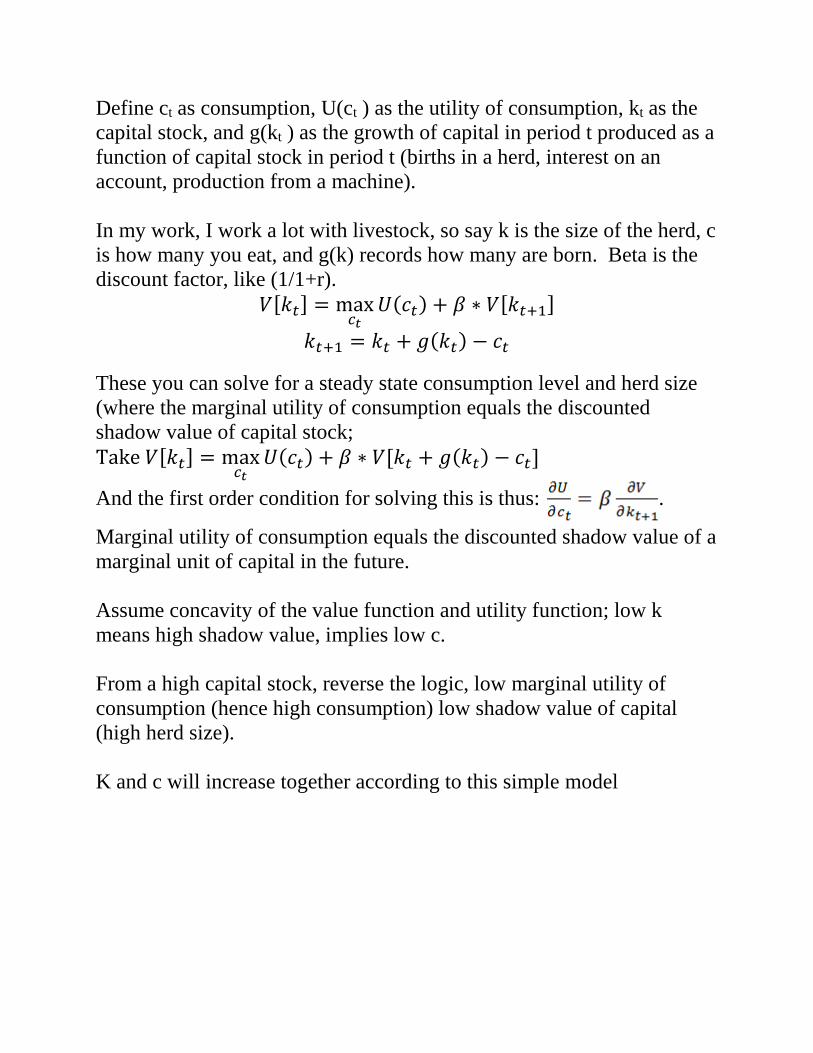
Define ct as consumption, U(ct ) as the utility of consumption, kt as the capital stock, and g(kt ) as the growth of capital in period t produced as a function of capital stock in period t (births in a herd, interest on an account, production from a machine). In my work, I work a lot with livestock, so say k is the size of the herd, c is how many you eat, and g(k) records how many are born. Beta is the discount factor, like (1/1+r).

𝑉𝑉[𝑘𝑘𝑡𝑡] = max𝑐𝑐𝑡𝑡

𝑈𝑈(𝑐𝑐𝑡𝑡) + 𝛽𝛽 ∗ 𝑉𝑉[𝑘𝑘𝑡𝑡+1]

𝑘𝑘𝑡𝑡+1 = 𝑘𝑘𝑡𝑡 + 𝑔𝑔(𝑘𝑘𝑡𝑡) − 𝑐𝑐𝑡𝑡 These you can solve for a steady state consumption level and herd size (where the marginal utility of consumption equals the discounted shadow value of capital stock; Take 𝑉𝑉[𝑘𝑘𝑡𝑡] = max

𝑐𝑐𝑡𝑡𝑈𝑈(𝑐𝑐𝑡𝑡) + 𝛽𝛽 ∗ 𝑉𝑉[𝑘𝑘𝑡𝑡 + 𝑔𝑔(𝑘𝑘𝑡𝑡) − 𝑐𝑐𝑡𝑡]

And the first order condition for solving this is thus: .

Marginal utility of consumption equals the discounted shadow value of a marginal unit of capital in the future. Assume concavity of the value function and utility function; low k means high shadow value, implies low c. From a high capital stock, reverse the logic, low marginal utility of consumption (hence high consumption) low shadow value of capital (high herd size). K and c will increase together according to this simple model

Now go back to the Markov state equation.

With 𝑘𝑘𝑡𝑡+1 = 𝑘𝑘𝑡𝑡 + 𝑔𝑔(𝑘𝑘𝑡𝑡) − 𝑐𝑐𝑡𝑡

for a given k, there is one value of c such that g(k)=c, so that kt+1 =kt (with other values of c being either larger or smaller than the growth in the herd for that k – and note a higher value of k will have higher c associated with the point where g(k)=c)

If the ct that solves for a given kt+1 is greater than the c that is equal to g(kt), herd size decreases from time t to time t+1 as consumption is greater than growth and you eat into existing capital stock.

If the ct that solves for a given kt+1 is less than the c that is equal to g(kt), herd size increases from time t to time t+1 as consumption is less than growth and you have some growth left after consumption to add to capital stock.

If the ct that solves for a given kt+1 is equal to the c that makes c equal to g(kt), herd size is unchanged from time t to time t+1 as consumption equals growth and I can call this (c,k) configuration the steady state and denote them (c*,k*). Say I want to make it more complicated by adding in something to represent the impact on the natural resource base. Rangeland evolves in response to stocking pressure, such that yt+1 =yt+f(yt, ∑ 𝑘𝑘𝑖𝑖𝑡𝑡𝑁𝑁

𝑖𝑖=1 ) Then we get a model with two state variables and one choice variable. “Phase diagram”, leading to steady state y, k, and c. An equilibrium

exists when there is nothing internal to the model that will bring about more change over time. Repeat adding complications. Tradeoff between parsimony and realism. We will look in a few minutes at a Solow model, which is a dynamic model of economic growth.

Structural Change

Lewis (1950’s). Two sector model. There is a traditional, agrarian, overpopulated rural subsistence sector. The marginal product of labor in this sector is zero (or close enough). Land and technology are fixed. For this reason, there is surplus labor in the rural sector. All laborers, whether surplus or otherwise, share in the agricultural output equally. Hence the return to labor in this sector is the average product, not the marginal product. The job of development is to draw this labor from the traditional sector to the industrial sector. Labor transfer brings about growth in output. The speed of the transfer is determined by industrial investment and capital accumulation in the modern sector.

Some problems here:

1) What if profit is not reinvested in capital, or is reinvested in labor saving technology?

2) Surplus labor in rural areas and full employment in urban areas?

3) Wages in the industrial sector remain constant as labor supply in this sector increases?

Talk through figure 3.1

Growth Theory with capital accumulation.

Drawing on chapter 3 of Todaro and Smith.

Stages of growth (non-communist manifesto). Rostow. 1960’s.

a) Traditional society. b) Preconditions stage. Transport develops, specialize production.

Ag improves to feed urban population. Availability of goods and capital from outside the country.

c) Takeoff. Net investment increases to over 10%. At least one manufacturing sector grows rapidly. A political, social, and institutional framework emerges.

d) Drive to maturity. Sustained period of growth. e) The age of mass consumption. The entire world arrives at OECD

standard consumption levels.

Leave alone the predictive power, it did not hang together as economic history. Very influential in the state department, post-Marshall plan, cold war setting. Justify transfer of capital.

Harrod-Domar

Size of total capital stock is K

Total GNP is Y

This allows us to define a Capital –Output ratio k = K/Y

Also, assume there is a fixed proportion of national income that is used as savings: a savings ratio s. Then we know that savings S = s*Y. These come from a Keynesian foundation: the marginal propensity to save (s) and the Incremental Capital-Output Ratio (ICOR). Some work with the model (and assuming savings equals investment in our closed economy) follows. The main insight is that:

∆𝑌𝑌𝑌𝑌

= 𝑠𝑠𝑘𝑘, so that growth in the national income depends on the ratio

of the savings rate to the capital output ratio. Say we have a capital-output ratio of 3, and a savings rate of 6%, we will get 2% GNP growth. If we save 15% with the same capital output ratio, we will get 5% growth. Leads to an idea of a “financing gap”. We set a target growth rate, we look at the capital –output ratio, then look at domestic savings. This tells us how much outside capital is needed.

Easterly (2002) notes that:

1) This was never meant as a growth model – it was meant to

comment on business cycles in the context of the aftermath of the Great Depression with high unemployment. When is an economy capable of steady growth at a constant rate?

2) It does not make all that much sense as a growth model (production capacity is proportional to the stock of machinery – more on this later).

3) Domar himself said it was not sensible as a long run growth model.

But still it was used, leading to a “capital constraint” / “capital fundamentalism” approach to growth and development. Solow, who we go to next, pointed out that this model requires the economy to lie on a “knife’s edge”. For a given savings rate and capital output ratio (and labor force growth rate implicitly), there is a defined growth rate for the economy. There is no reason to assume this will be a stable equilibrium, as given the particular parameter configuration the economy could veer off into unemployment (not enough machines for the people) or it could veer in the other direction to labor shortage and inflation (not enough people for the machines). No real clarity on how the parameters would change from one direction to another either. Labor force growth is not endogenous to the model.

Solow (1988) said that he developed his theory in response to HD, since he felt something was wrong with the workings of the model. “An expedition from Mars arriving on Earth, having read this literature, would have expected to find only the wreckage of a capitalism that had shaken itself to pieces long ago. Economic history was indeed a record of fluctuations as well as of growth, but most business cycles seemed to be self-limiting. Sustained, though disturbed, growth was not a rarity”

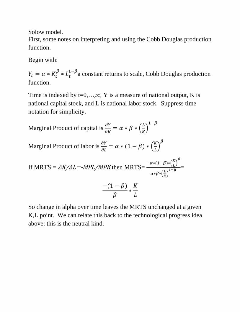
Solow model. First, some notes on interpreting and using the Cobb Douglas production function.

Begin with:

𝑌𝑌𝑡𝑡 = 𝛼𝛼 ∗ 𝐾𝐾𝑡𝑡𝛽𝛽 ∗ 𝐿𝐿𝑡𝑡

1−𝛽𝛽a constant returns to scale, Cobb Douglas production function.

Time is indexed by t=0,…,∞, Y is a measure of national output, K is national capital stock, and L is national labor stock. Suppress time notation for simplicity.

Marginal Product of capital is 𝜕𝜕𝑌𝑌𝜕𝜕𝜕𝜕

= 𝛼𝛼 ∗ 𝛽𝛽 ∗ �𝐿𝐿𝜕𝜕�1−𝛽𝛽

Marginal Product of labor is 𝜕𝜕𝑌𝑌𝜕𝜕𝐿𝐿

= 𝛼𝛼 ∗ (1 − 𝛽𝛽) ∗ �𝜕𝜕𝐿𝐿�𝛽𝛽

If MRTS = ∆K/∆L=-MPL/MPK then MRTS= −𝛼𝛼∗(1−𝛽𝛽)∗�𝐾𝐾𝐿𝐿�

𝛽𝛽

𝛼𝛼∗𝛽𝛽∗�𝐿𝐿𝐾𝐾�1−𝛽𝛽 =

−(1 − 𝛽𝛽)𝛽𝛽

∗𝐾𝐾𝐿𝐿

So change in alpha over time leaves the MRTS unchanged at a given K,L point. We can relate this back to the technological progress idea above: this is the neutral kind.

Next, use the assumption that the rent paid to capital r and the wage paid to labor w are equal to the value of the marginal product, or in this case since Y is already in ‘value’ terms, marginal product or capital and marginal product of labor.

If r=MPK= 𝛼𝛼 ∗ 𝛽𝛽 ∗ �𝐿𝐿𝜕𝜕�1−𝛽𝛽

, and K units of capital are used, r*K is the share of national output that is returned to capital. Here, we can multiply it out and see:

r*K=MPK*K = (𝛼𝛼 ∗ 𝛽𝛽 ∗ �𝐿𝐿𝜕𝜕�1−𝛽𝛽

) ∗ 𝐾𝐾= 𝛼𝛼 ∗ 𝛽𝛽 ∗ (𝐿𝐿)1−𝛽𝛽 ∗ 𝐾𝐾𝛽𝛽−1 ∗ 𝐾𝐾1 =

𝛽𝛽 ∗ �𝛼𝛼 ∗ 𝐾𝐾𝛽𝛽 ∗ (𝐿𝐿)1−𝛽𝛽� = 𝜷𝜷 ∗ 𝒀𝒀

Same kind of story with labor and the wage rate:

w*L=MPL*L= is (𝛼𝛼 ∗ (1 − 𝛽𝛽) ∗ �𝜕𝜕𝐿𝐿�𝛽𝛽

) ∗ 𝐿𝐿= 𝛼𝛼 ∗ (1 − 𝛽𝛽) ∗ 𝐿𝐿−𝛽𝛽 ∗ 𝐾𝐾𝛽𝛽 ∗

𝐿𝐿1 = (1 − 𝛽𝛽) ∗ �𝛼𝛼 ∗ 𝐾𝐾𝛽𝛽 ∗ 𝐿𝐿1−𝛽𝛽� = (𝟏𝟏 − 𝜷𝜷) ∗ 𝒀𝒀

The beta then can be interpreted as the share of national income that is allocated to owners of capital and the rest is the share that is allocated to labor.

Finally, a feature used by Solow is the constant returns to scale. With CRS, γ*f(K,L)=f(γ*K,γ*L). So here let gamma equal two for example,

2 ∗ 𝑌𝑌 = 𝛼𝛼 ∗ (2 ∗ 𝐾𝐾)𝛽𝛽 ∗ (2 ∗L)1-β Solow points out that if you can use γ=2, you can use γ =1/L for example, and state it in output per worker and capital per worker.

Solow model in full:

Let Y equal national income, say GNI.

Let L equal the size of the labor force and for our purposes the population.

Let K equal the capital stock – the number of machines for example.

Let the relationship between Y,L, and K be defined as:

𝑌𝑌𝑡𝑡 = 𝛼𝛼 ∗ 𝐾𝐾𝑡𝑡𝛽𝛽 ∗ 𝐿𝐿𝑡𝑡1−𝛽𝛽a CRS Cobb Douglas production function.

Alpha can be thought of as the stock of technological knowledge, Beta is the share of national income that is returned to owners of capital, and (1-Beta) is the share of national income that is returned to laborers (as we saw above).

These are given as parameters. We know from this interpretation that Beta has to lie in the interval [0,1].

If 𝑌𝑌𝑡𝑡 = 𝛼𝛼 ∗ 𝐾𝐾𝑡𝑡𝛽𝛽 ∗ 𝐿𝐿𝑡𝑡1−𝛽𝛽is CRS, then γ*f(K,L)=f(γ*K,γ*L) so if we

choose gamma to be (1/L), we end up with y=α*kβ where y=(Y/L) and k=K/L. Note that by assumption, this has diminishing marginal returns to k, which we now interpret as capital per worker.

Let s be the savings rate of national income, so that total national savings and we assume investment=s*Y, and savings / investment per worker equals s*y. Savings shows up as more machines per worker next period.

What is left of national income after we take out savings is c, consumption. So (1-s)*y is consumption per laborer or per person as we are treating it.

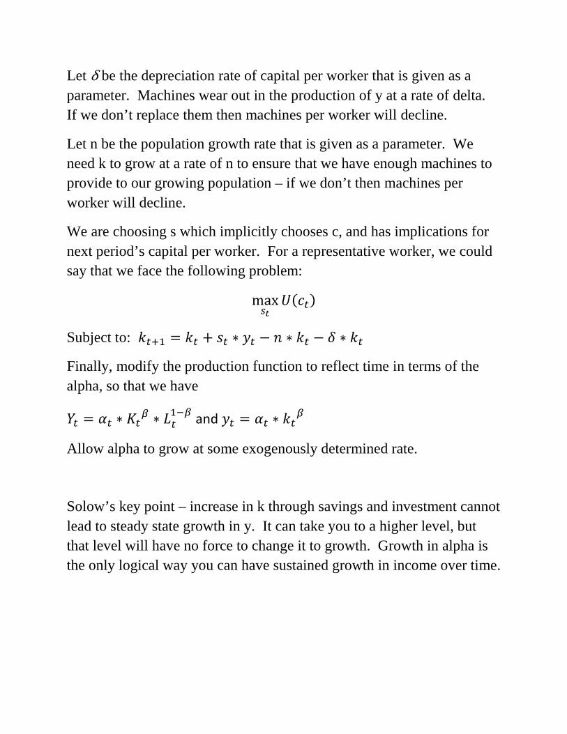
Let δ be the depreciation rate of capital per worker that is given as a parameter. Machines wear out in the production of y at a rate of delta. If we don’t replace them then machines per worker will decline.

Let n be the population growth rate that is given as a parameter. We need k to grow at a rate of n to ensure that we have enough machines to provide to our growing population – if we don’t then machines per worker will decline.

We are choosing s which implicitly chooses c, and has implications for next period’s capital per worker. For a representative worker, we could say that we face the following problem:

max𝑠𝑠𝑡𝑡

𝑈𝑈(𝑐𝑐𝑡𝑡)

Subject to: 𝑘𝑘𝑡𝑡+1 = 𝑘𝑘𝑡𝑡 + 𝑠𝑠𝑡𝑡 ∗ 𝑦𝑦𝑡𝑡 − 𝑛𝑛 ∗ 𝑘𝑘𝑡𝑡 − 𝛿𝛿 ∗ 𝑘𝑘𝑡𝑡

Finally, modify the production function to reflect time in terms of the alpha, so that we have

𝑌𝑌𝑡𝑡 = 𝛼𝛼𝑡𝑡 ∗ 𝐾𝐾𝑡𝑡𝛽𝛽 ∗ 𝐿𝐿𝑡𝑡1−𝛽𝛽 and 𝑦𝑦𝑡𝑡 = 𝛼𝛼𝑡𝑡 ∗ 𝑘𝑘𝑡𝑡

𝛽𝛽

Allow alpha to grow at some exogenously determined rate.

Solow’s key point – increase in k through savings and investment cannot lead to steady state growth in y. It can take you to a higher level, but that level will have no force to change it to growth. Growth in alpha is the only logical way you can have sustained growth in income over time.

Formally:

max𝑠𝑠𝑡𝑡

𝑈𝑈(𝑐𝑐𝑡𝑡)

Subject to: 𝑘𝑘𝑡𝑡+1 = 𝑘𝑘𝑡𝑡 + 𝑠𝑠𝑡𝑡 ∗ 𝑦𝑦𝑡𝑡 − 𝑛𝑛 ∗ 𝑘𝑘𝑡𝑡 − 𝛿𝛿 ∗ 𝑘𝑘𝑡𝑡

Or : 𝑘𝑘𝑡𝑡+1 = 𝑘𝑘𝑡𝑡 + 𝑠𝑠𝑡𝑡 ∗∝𝑡𝑡∗ 𝑘𝑘𝑡𝑡𝛽𝛽 − 𝑛𝑛 ∗ 𝑘𝑘𝑡𝑡 − 𝛿𝛿 ∗ 𝑘𝑘𝑡𝑡

With 𝑐𝑐𝑡𝑡 = (1 − 𝑠𝑠𝑡𝑡) ∗ 𝛼𝛼𝑡𝑡 ∗ 𝑘𝑘𝑡𝑡𝛽𝛽

Steady State Diagram looks like this with y on the y-axis and k on the x-axis.

Critical of the idea of a fixed “capital – output ratio”.

Solow (1957) is looking at aggregate production function. Think of the whole economy of a nation as a big production function, mixing capital and labor to produce income.

Empirically, he finds some sources for the US economy from 1909 to 1949 that allow him to fill in this relationship and solve for the technical change index (setting 1909 to 1 arbitrarily). Log transform both sides, purge output series of technical change, and regress: yt/αt = 0.48*kt

0.353 R squared =0.9996

He suggests over the 40 year period, output per labor hour doubled, and output shifted upward about 80%. He argues 1/8th of this is attributable to increased capital per man hour, 7/8ths of this is due to technical change. Critical here is diminishing returns to capital – note this will be important for convergence ideas. So the main point here is that the technical change index is accounting for the vast majority of growth, not increased use of capital. This is how he assesses the US growth experience during this time period. Where does change to the technical change index come from? Solow was not looking at that. Technical change was growing exogenously, at 1.5% per year.

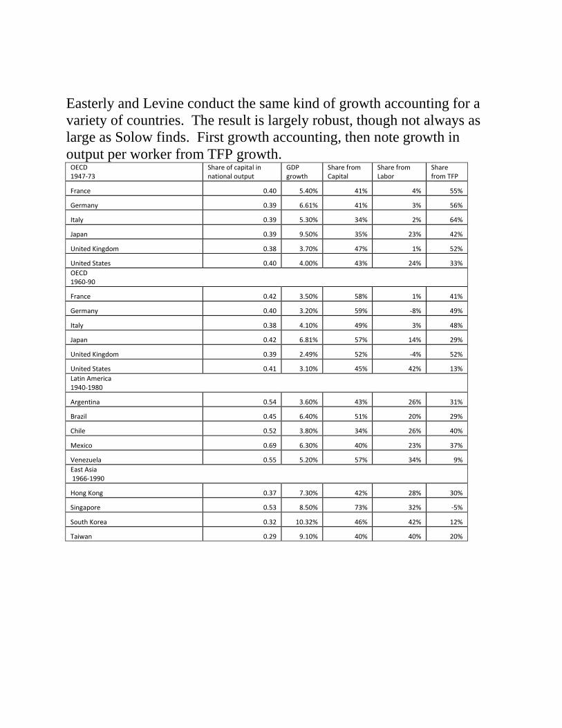
Easterly and Levine conduct the same kind of growth accounting for a variety of countries. The result is largely robust, though not always as large as Solow finds. First growth accounting, then note growth in output per worker from TFP growth.

OECD 1947-73

Share of capital in national output

GDP growth

Share from Capital

Share from Labor

Share from TFP

France 0.40 5.40% 41% 4% 55% Germany 0.39 6.61% 41% 3% 56% Italy 0.39 5.30% 34% 2% 64% Japan 0.39 9.50% 35% 23% 42% United Kingdom 0.38 3.70% 47% 1% 52% United States 0.40 4.00% 43% 24% 33% OECD 1960-90 France 0.42 3.50% 58% 1% 41% Germany 0.40 3.20% 59% -8% 49% Italy 0.38 4.10% 49% 3% 48% Japan 0.42 6.81% 57% 14% 29% United Kingdom 0.39 2.49% 52% -4% 52% United States 0.41 3.10% 45% 42% 13% Latin America 1940-1980 Argentina 0.54 3.60% 43% 26% 31% Brazil 0.45 6.40% 51% 20% 29% Chile 0.52 3.80% 34% 26% 40% Mexico 0.69 6.30% 40% 23% 37% Venezuela 0.55 5.20% 57% 34% 9% East Asia 1966-1990 Hong Kong 0.37 7.30% 42% 28% 30% Singapore 0.53 8.50% 73% 32% -5% South Korea 0.32 10.32% 46% 42% 12% Taiwan 0.29 9.10% 40% 40% 20%

How one views TFP is what leads to the distinction between (what could be called) exogenous and endogenous growth theory. Endogenous growth theory / new growth theory looks at what causes technical change.

Before we get to endogenous growth theory, let us consider the decreasing marginal returns to capital result.

What does that imply in terms of convergence? Why could this lead to the conclusion that funding and aid could lead to income growth?

1) Technology transfer. Can skip stages (no need for land lines,

jump to mobile phones). Replicate technology, not do the R&D. Leapfrog. The technology gap is assumed away. The alphas converge.

2) The marginal product of capital (and profitability of investments) are lower where capital intensity is higher. Diminishing marginal returns to capital. Capital has a higher impact on productivity where capital is scarce, as is the case in the developing countries.

Incomes should tend to converge in the long run due to these two factors. This can be called unconditional convergence to contrast with… Conditional convergence. Convergence conditional upon key variables such as population growth, savings, political stability,…

Evidence on unconditional convergence. See figure 2.8 in the book, or figure 1 in the Barro article (1991).

Unconditional convergence for similar kinds of environments (OECD countries, US states). Not found for world sample. Barro article as an example of conditional convergence.

Human capital as a variable. Secondary and primary enrollment rates as well as initial values of GDP per capita as variables. With these variables in there, higher starting income per capita is negatively related to growth. Each $1,000 increase in starting GDP per capita reduces the real growth rate (per capita) by 0.75% per year. Per capita growth is positively related to initial human capital. Also look at student teacher ratios, find higher ratio is negatively correlated with growth. Holding human capital constant, we have evidence in the article of convergence across countries across time.

A large literature develops around this theme, often using the Penn World table: http://www.rug.nl/research/ggdc/data/pwt/

A related set of studies looks at the impact of policy on growth:

Note Easterly and Rebelo (1993) Journal of Monetary Economics, King and Rebelo (1990) JPE, Gale and Easterly (1995) for more in depth analysis of how fiscal policy influences economic growth. Basic answer – it is complicated.

Overall: poor countries tend to catch up to rich countries if their human capital levels are high. Countries with high levels of human capital have lower fertility rates and higher ratios of investment to GDP.

As always, keep in mind that correlation is not causation. And note distribution of income studies such as Xala-i-Martin’s.

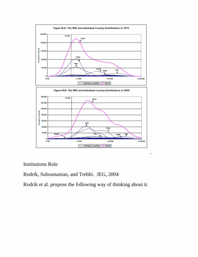
Institutions Rule

Rodrik, Subramanian, and Trebbi. JEG, 2004

Rodrik et al. propose the following way of thinking about it.

And they also give us the following empirical pattern where the first row presents a version of institutions (the governance indicator ‘rule of law’), the second is a version of integration (openness to trade), and the third is geography (distance from the equator). All have log income per capita on the y axis.

“Institutions rule” is their empirical finding (and title).

Introduction identifies three ‘strands of thought’ on what leads to differences in income levels over time.

Geography: climate, natural resource endowment, disease burden, transport costs, diffusion of knowledge and technology.

International trade / market integration. Moderate or maximal version, stressing the maximal version ‘…that trade / integration is a major determinant of whether poor countries grow or not.’ (p. 132)

Institutions. Property rights and the rule of law. Social infrastructure, rules of the game…

Growth theory is about accumulation: physical capital, human capital, and technological change. Countries differ in their rates of accumulation. Why?

Quality of institutions is likely endogenous (an outcome as well as an input to other outcomes).

Integration with the world economy is likely endogenous.

Trade endogeneity we often deal with using a gravity model of trade in international economics. This model predicts bilateral trade flows based on the economic sizes of (often using GDP measurements) and distance between two countries. The basic theoretical model for trade flow between two countries (call them i and j) takes the form of:

Where F is the trade flow from i to j, M is the economic mass of each country, D is the distance and G is a constant. (modified from the Wikipedia description) .

This can be used as an instrument for observed flows.

Frankel and Romer (1999), first regress bilateral trade flows as a share of GDP on measures of country mass, distance between trading partners, other geographical variables to construct ‘trade hat’. This constructed one is used in place of the actual one.

Colonial mortality rates are used as an instrument for institutional quality. To expand the data set, they also use as instruments fractions of the population speaking English and Western European languages as a first language. Institution ‘hat’. Regress observed institutional quality on these and use the estimate that is purged of the endogeneity.

“The research agenda to which this paper contributes is one that clarifies the priority of pursuing different objectives – improving the quality of domestic institutions, achieving integration into the world economy, or overcoming geographical adversity – but says very little about how each one of these is best achieved.” P 136

GDP per capita in 1995 (by PPP).

Institutional Quality using Kaufmann’s (KK, or KKM, or KKZ sometimes)

Integration is the ratio of trade to GDP.

Geography is distance from the equator.

log(𝐺𝐺𝐺𝐺𝐺𝐺 𝑝𝑝𝑝𝑝𝑝𝑝 𝑐𝑐𝑐𝑐𝑝𝑝𝑐𝑐𝑐𝑐𝑐𝑐) = 𝑐𝑐𝑛𝑛𝑐𝑐𝑝𝑝𝑝𝑝𝑐𝑐𝑝𝑝𝑝𝑝𝑐𝑐 + 𝛼𝛼 ∗ 𝐼𝐼𝐼𝐼𝐼𝐼� + 𝛽𝛽 ∗ 𝐼𝐼𝐼𝐼𝐼𝐼� + 𝛾𝛾 ∗ 𝐺𝐺𝐺𝐺𝐺𝐺

First stage regression, regress institutional index on settler mortality / language, the constructed trade measure and geography. That which can be explained by these three variables; the indirect impact of geography and trade, and institutional quality as correlated with this language / mortality indicator.

SM and CONST do not appear in the second stage, thus satisfying the ‘exclusion restrictions’.

Large impact of institutions.

Regress the observed trade openness on geography and constructed openness, regress the observed institutional quality variable on settler mortality and geography. Taking out the cross effect in table three, looking at ‘own’ instrument only.

Page 144.

Page 147

“How much guidance do our results provide to policymakers who want to improve the performance of their economies? Not much at all. Sure, it is helpful to know that geography is not destiny, or that focusing on increasing the economy’s links with world markets is unlikely to yield convergence. But the operational guidance that our central result on the primacy of institutional quality yields is extremely meager.” (p. 157)

New Growth Theory. Growth based on spillovers and coordination (new growth theory in chapter four) As we talked about last time, there are two main findings we have come upon as we looked at the development of growth models.

1) Growth in technology (better ways of doing things) rather than more factor inputs appears to play the larger role in growth.

2) The implication that Solow’s diminishing marginal returns to capital finding implies income will converge over time across nations is not empirically supported.

With regard to the first point, it is not satisfactory to think of technological progress as some exogenous force.

Incentives do not influence the rate of technological progress?

How do we explain the fact that the rate of progress appears to vary across countries?

Are there identifiable structural factors that explain the variation?

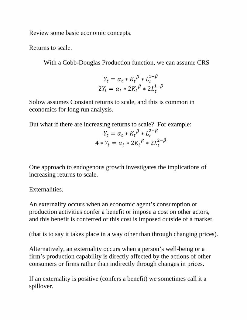
Review some basic economic concepts. Returns to scale.

With a Cobb-Douglas Production function, we can assume CRS

𝑌𝑌𝑡𝑡 = 𝛼𝛼𝑡𝑡 ∗ 𝐾𝐾𝑡𝑡𝛽𝛽 ∗ 𝐿𝐿𝑡𝑡

1−𝛽𝛽 2𝑌𝑌𝑡𝑡 = 𝛼𝛼𝑡𝑡 ∗ 2𝐾𝐾𝑡𝑡𝛽𝛽 ∗ 2𝐿𝐿𝑡𝑡

1−𝛽𝛽

Solow assumes Constant returns to scale, and this is common in economics for long run analysis. But what if there are increasing returns to scale? For example:

𝑌𝑌𝑡𝑡 = 𝛼𝛼𝑡𝑡 ∗ 𝐾𝐾𝑡𝑡𝛽𝛽 ∗ 𝐿𝐿𝑡𝑡2−𝛽𝛽

4 ∗ 𝑌𝑌𝑡𝑡 = 𝛼𝛼𝑡𝑡 ∗ 2𝐾𝐾𝑡𝑡𝛽𝛽 ∗ 2𝐿𝐿𝑡𝑡2−𝛽𝛽

One approach to endogenous growth investigates the implications of increasing returns to scale. Externalities. An externality occurs when an economic agent’s consumption or production activities confer a benefit or impose a cost on other actors, and this benefit is conferred or this cost is imposed outside of a market. (that is to say it takes place in a way other than through changing prices). Alternatively, an externality occurs when a person’s well-being or a firm’s production capability is directly affected by the actions of other consumers or firms rather than indirectly through changes in prices. If an externality is positive (confers a benefit) we sometimes call it a spillover.

Think of technology as having some aspects of a public good (non rival, non excludable). One explanation of what causes progress could be the role of science in an economy. Where there are a lot of scientists, there will be a lot of innovation. Targeted education, research universities,…. This would push it towards the public good realm, and have some obvious policy implications. Another idea is that innovation and progress occur where the returns to such efforts are the highest. Profitability is the key, so those countries that offer the highest profit will have innovations tailored to their needs. This would suggest that rather than a public good model, we need to make sure the market for innovations works efficiently. Looking at technological progress related to key variables (population growth, investment, government policy, education levels, trade policy, types of education, structure of the economy,…) leaves the impression that there are a variety of factors that influence the rate of technological progress.

One way to capture the basics of this approach that builds on the Solow model is a Romer model based on increasing returns to scale due to capital spillovers. Growth process at firm level. There are spillovers, positive benefits, conferred on other firms by an individual firm’s capital stock. Define an economy wide average capital stock per firm as 𝑘𝑘�. Modify the basic Solow model we looked at for firm i.

𝑌𝑌𝑖𝑖𝑡𝑡 = 𝛼𝛼𝑖𝑖𝑡𝑡 ∗ 𝐾𝐾𝑖𝑖𝑡𝑡𝛽𝛽 ∗ 𝐿𝐿𝑖𝑖𝑡𝑡1−𝛽𝛽

where i is an index for the firms in the economy and Y is output by the firm, K is capital at the firm, and L is labor at the firm. Instead of taking technological progress as given, try making it a function:

𝛼𝛼𝑖𝑖𝑡𝑡 = 𝐴𝐴 ∗ 𝑘𝑘𝑡𝑡𝜌𝜌����

Note for the firm, there are constant returns to scale in own capital and labor. However, the presence of a positive externality from other firms’ capital stock leads to overall increasing returns to scale. Assume for simplicity that all firms are identical, and you get:

𝑌𝑌𝑖𝑖𝑡𝑡 = 𝐴𝐴 ∗ �̅�𝑘𝜌𝜌𝑐𝑐 ∗ 𝐾𝐾𝑖𝑖𝑡𝑡𝛽𝛽 ∗ 𝐿𝐿𝑖𝑖𝑡𝑡1−𝛽𝛽 = 𝐴𝐴 ∗ 𝐾𝐾𝑖𝑖𝑡𝑡𝛽𝛽+𝜌𝜌 ∗ 𝐿𝐿𝑖𝑖𝑡𝑡

1−𝛽𝛽 So this model implies that the spillover effect of the firm’s capital accumulation decision leads to economywide benefits, and this could explain “the residual”. This could explain the failure to find “unconditional convergence”.

Strategic interactions and Game theory. Game theory is a tool to understand why outcomes with higher payoffs may not be possible to obtain if each individual acts in his or her own best interest. How we understand why a failure to coordinate actions when there are strategic actions leads us to an outcome that does not maximize welfare of the decision makers. A set of strategies is a Nash equilibrium if, holding the strategies of all other players constant, no play can obtain a higher payoff by choosing a different strategy. Complementarities, coordination, and commitment. There is you and there is me in a rural area. We both grow maize and eat it. I am considering buying a pickup truck and moving into transport. You are considering moving from maize into garden crops. There is a town some distance away where you could sell your garden crops if you hire my transport, and we could both buy maize there cheaper. Right now, both growing maize, we earn $1 per person per day (WB poverty line). If I invest in the pickup truck and you don’t switch to gardening, you get some free rides to town and benefit but I lose since there is nobody to pay me to take crops to market (you go to $1.50 and I drop to 0.50). If you switch to garden crops and I don’t buy the truck, I benefit by getting to trade you maize for carrots (thus getting $1.50 per day), but you lose since you get less food from you land ($0.50 per day).

If I buy the truck and you switch to garden crops, we both benefit and get $1.25 per day, so the overall economic activity increases from $2 to $2.50. Maize Transport

Maize 1, 1 1½, ½

Garden Crops ½, 1½ 1 ¼ ,1¼ Nash best response leads to Maize-Maize as outcome, when both would be better off if moving to Garden Crops – Transport. Simple model, and repeated interactions can lead to resolution of such problems, but the basic idea carries into more complicated settings where coordination failures may be much harder to resolve. Education. Firms will not invest in an area if there are low education levels. Students will not pay for the education the firms want unless there is some chance of getting a job with these firms. If you do get the education, migrate to where firm is.

Big Push model. Rosenstein-Rodan (and Krugman’s discussion of it). Spillovers exist here in that a firm’s industrial laborers are paid a higher wage than in the traditional sector, thus creating a market for manufactured goods. Here, the nature of the spillover originates in the idea of demand creation – your workers are the market for the output produced by other firms.

1) Assume there is only one factor of production – Labor. 2) Labor has two sectors. Traditional and modern. Wages are higher

in modern sector. 3) There are N types of products, and N is “large”. Either traditional

or modern sector can produce a given product. A modern sector worker is more productive than a traditional sector worker, but only if a substantial fixed cost is first paid by the modern firm.

4) The traditional sector has constant returns, the modern sector has increasing returns.

5) Each product receives a constant and equal share of consumption. (national income of Y is split over the N goods Y/N)

6) The economy is closed – not international supply or demand. 7) Perfect competition in the traditional sector. Modern producer

enters as modern sector monopolist, but will face competitive conditions since traditional sector can produce if prices raised to monopoly level.

How will such a producer price? She cannot raise her price as much as she would like. The reason is that potential competition from the traditional sector puts a limit on the price: she cannot go above a price of 1 (in terms of traditional labor) without being undercut by traditional producers. So each producer in the modern sector will set the same price, unity, as would have been charged in the traditional sector.

Figure 1

Assume selling price is one, so revenue is the same as output. For the traditional firm, the wage is one and the selling price is one, so revenue equals costs at all points on “traditional”.

If no sector industrializes, we stay at q1 with traditional production.

One sector will industrialize when there is profit from doing so. Graphically, if the wage bill in the modern sector lies below the production function (since both selling price and input price of labor are one).

The failure to coordinate comes in if the wage bill lies between the modern sector and traditional sector production functions.

Start with a subsistence economy. No export possibility. If I industrialize, who is going to buy my product? My workers, but I need more of a market than just them. But how do we get started, since there is little to make me move first? Demand for each good is Y/N, but if

other sectors don’t modernize, then there is not enough demand to buy my product. Given the fixed cost of entry, a modern firm will decide to enter into a market producing a given product depending on

1) How much more efficient is modern sector production. 2) How much more expensive is labor in the modern sector.

A variation on this theme is spillovers based on “agglomeration economies”. This goes back to the concept of linkages introduced above. Production costs for a firm decline when related firms are located near each other (Detroit, Silicon Valley). 2% of US land area accounts for over 50% of GDP. From Easterly and Levine.

We will revisit the idea later, but this is expands on the idea of linkages: forward linkages and backward linkages.

The O-Ring Theory is based on the concept of positive assortive matching. In modern production, many activities must be done well together in order for any of them to result in high value. Strong complementarity resulting from specialization and division of labor. Divide production of a given good into n different tasks. Each task can be done at a skill level of q, where q is between zero and 1. The output is the mutiplicitive product of the q values. Positive assortive matching. Workers with high skills will work together, low skills together. If you are high type, you want to work with other high types, so you go there. Low types left. Also, since high types get higher wages if the labor market is working, they can be drawn to more productive firms by higher wages. Think about two firms, and four workers to split between the two firms. We have a q=.25, q=.5, q=.75, and q=1 worker. We make output Y by multiplying the value of each worker’s q.

where i and j can be (.25, .5. .75, or 1), and you can only use a worker in making one thing and there is only one kind of each worker. 0.25 0.50 0.75 1.00 0.25 NP 0.125 0.1875 0.25 0.50 See other side NP 0.375 0.50 0.75 See other side See other side NP 0.75 1.00 See other side See other side See other side NP

Here is a list of the y levels that occur by mixing each possible pairing of the q’s. Mix (.25, .5) and (.75, 1) get (.125) and (.75) for a total .875

Mix (.25,1) and (.5,.75) get (.25) and (.375) for a total .625 Mix (.25,.75) and (.5,.1) get (.188) and (.5) for a total .688

Total output is highest by putting the two highest together (.75+.125 =.875) than by putting the highest and the lowest and the middle two (.25 + .375=.625) or the highest and the second and the other two (.5+.188=.688). One interpretation is that like will flow to like as the wages will be higher for those paired with higher productivity workers. Look at multiplicative production function: the marginal product of a given worker is defined by the q of the other worker in the pair. Assuming workers are paid the value of their marginal product, wages are higher when your partner is higher skill. Alternatively think of skill improvement. Suppose it costs 0.03 units of output to improve the q level of a worker through a training program by 0.05. The low firm (with the .25 and the .5) pays .03 worth of output to increase the q of a worker, it could increase the quality of the .25 worker to .3, output goes up from (.25*.5) or .125 to (.3*.5) or .15 – a gain of .025 (if they invest in the more productive guy, it goes up 0.0125). The benefits are outweighed by the cost. The high firm (with the .75 and the .5) pays .03, increases the .75 person up to .8, product goes up from (.75*1) or .75 to (.8*1)= .8, an increase of .05. Here the benefits of .05 outweigh the costs of .03.

Investment in workers in the firm with the higher productivity people to begin with (or in a similar fashion, will hire away other workers with higher skill). In a similar fashion, you can analyze why decisions to invest in human capital (to increase one’s own q level) relies on the q levels of those around you. You need the complementarity for this to work – the multiplicative production function. You also need heterogeneity in workers. This also can be used to explain brain drain if you modify it some. “If strategic complementarity is sufficiently strong, microeconomically identical nations or groups within nations could settle into equilibria with different levels of human capital”

A related issue is the commitment problem. What is the commitment problem? The firm promises to invest if people get education, they do, and the firm does not live up to its promise. Why did Odysseus get tied to the mast and fill his sailors’ ears with wax when he wanted to hear the song of the sirens? What you commit to ex ante has to be credible ex post. Coordination problems when actions are based on a announced strategy that may not be the strategy implemented. Greif et al contrasts a cartel explanation (the guild formed to create cartel returns for members) with a commitment explanation (the institution was needed to allow trade to happen at all). The two players are: Rulers (location specific and provide security to out of town traders). Traders (come from out of town and allow trade which has benefits for both the traders and the rulers).

Avner Grief is an economist who studies the rise of medieval trade in the Mediterranean basin. He describes the following situation:

• A ruler of a city state can offer security to a visiting merchant. The ruler can protect the merchant from being robbed by the citizens of the city state at a cost of 1.

• The merchant has goods that cost him 1 to obtain elsewhere and transport to the city state if he decides to come. If they are sold in the city state, they earn revenue of 6, thus generating a profit of 5.

• The deal is that if the merchant comes with goods that generate a profit of 5 the ruler gets 2, the merchant keeps 3. The ruler thus nets 1 after paying the security cost [1 3 cell in the table]

• If the merchant does not come, no security costs are incurred; no goods are bought elsewhere to be sold in the city state, the ruler and the merchant get zero. [0 0 cell in the table]

• If the merchant comes and the ruler does not provide security, the ruler and his mob of citizens rob the stuff and sell it for profit of 6. The ruler keeps half (3), the mob keeps half (3). The merchant suffers a loss of -1. [3 -1 cell in the table]

• If the ruler pays for protection but the merchant does not come, the ruler pays the cost of protection, but gets no benefits, so suffers a loss of -1. [-1 0 cell in the table]

This can be summarized in the following table.

Merchant

Come Don’t Come

Ruler Protect 1 3 -1 0

Don’t protect 3 -1 0 0

If the security of the trader is violated (the ruler allows all his stuff to be stolen and lets his people get away with it), what can the traders do?

Bilateral reputation – the trader who is attacked does not come back.

Multilateral reputation – the trader and his group does not come back. Administrative bodies – no traders at all come back and any that do are detected and punished for doing so. An enforceable embargo. An example of getting institutions right to allow economic growth to happen. Consider how the structural adjustment process has to face the commitment problem.

So what have we found here?

We have new ways of looking at “poverty traps” – why things don’t converge, and what can cause a dualism to emerge. We can begin to trace growth back to resolution of coordination issues, and the failure of growth to an inability to coordinate. Understand how best response, economically rational decisions may not be optimal and may require outside intervention. Identify why government may be necessary, and also have a better idea of what types of efforts won’t work.