theoretical study of the trapped dipolar bose gas in the
TRANSCRIPT

Theoretical Study of the Trapped
Dipolar Bose Gas in the
Ultra-Cold Regime
Russell Bisset
a thesis submitted for the degree of
Doctor of Philosophyat the University of Otago, Dunedin,
New Zealand.
August 22, 2013

ii

Abstract
The work of this thesis concerns the properties of a Bose gas of polariseddipoles that have long-range and anisotropic interactions. Our work is di-vided into two parts. First, the stability of a dipolar Bose gas at finitetemperature (both above and below the critical Bose-Einstein condensa-tion (BEC) temperature Tc). Second, the fluctuations of a dipolar BECat zero and small finite temperature (T Tc) in a regime where rotonicexcitations emerge.
Part I
Stability of a Trapped Finite Temperature Dipolar Bose Gas:
Above Tc we implement a semiclassical Hartree-Fock theory and charac-terise the dependence of the stability boundary on temperature, trap ge-ometry and the strength of the dipole-dipole interaction and contact inter-action. We find that stability is greatly enhanced above Tc and that trapgeometry continues to play a key role. Furthermore, we find that for oblatetraps a novel double instability feature emerges.
To extend our stability analysis to the low temperature regime, T < Tc, wedevelop a beyond semiclassical Hartree theory. We use this to characterisethe stability boundary as a function of geometry. Interestingly, we findlarge beyond semiclassical effects above Tc for prolate trapping geometries.We characterise thermal effects on biconcave condensate states.
Part II
Rotons and Fluctuations in a Trapped Dipolar Condensate:
To study density fluctuations we implement a numerical scheme to solvethe Gross-Pitaevskii equation and the Bogoliubov de Gennes equations.We find that the phonon and roton gases spatially separate and we charac-terise the role of the anomalous density on the density fluctuations of thethermally activated rotons. We develop a numerical scheme that calculatesnumber fluctuations within cells of various shapes and sizes, and find astrong peak in the fluctuations when the cell size is around half the rotonwavelength, which should be detectable by current experiments. By tailor-ing the cell shape we predict that experiments should be able to detect the
iii

effects of individual roton modes.
For the study of zero temperature fluctuations we deploy the Gross-Pitaevskiiand Bogoliubov de Gennes equations to calculate the dynamic and staticstructure factors for a highly oblate BEC. We find a clear signature of theroton gas dispersion relation within the structure factors. This signatureshould be detectible in current experiments using Bragg spectroscopy.
iv

Acknowledgements
First and foremost, I would like to thank my supervisor, Associate ProfessorBlair Blakie. Not only is he an exceptional and inspirational physicist, buthe is also an incredibly good supervisor, placing the growth of his studentsas a high priority. Thank-you for your endless patience for my never-endingquestions, and for your guidance and clear-sighted wisdom.
I would like to thank Dr Danny Baillie for enjoyable and fruitful collabora-tions.
Thanks to Professor Rob Ballagh for all you’ve taught me and for yourguidance.
Thanks to Dr Andrew Martin, Sam Cormack, Dr Ashton Bradley, LukeSymes, Joseph Towers and Andrew Wade for many useful and interestingdiscussions.
Thank-you to Sandy Wilson for all your help.
Thanks to my parents for giving me the encouragement to follow my ownpath and for always believing in me.
Last but not least I would like to thank Jessie for her support, throughboth the good and the difficult times, thanks for being there for me.
v

vi

Contents
1 Introduction 1
1.1 Bose-Einstein Condensation . . . . . . . . . . . . . . . . . . . . . . . . 1
1.2 The Dipole-Dipole Interaction . . . . . . . . . . . . . . . . . . . . . . . 3
Hamiltonian . . . . . . . . . . . . . . . . . . . . . . . . . . . . . 4
Ferrofluids . . . . . . . . . . . . . . . . . . . . . . . . . . . . . . 5
1.3 Ultra-Cold Dipolar Systems . . . . . . . . . . . . . . . . . . . . . . . . 6
1.3.1 Electric Dipoles . . . . . . . . . . . . . . . . . . . . . . . . . . . 7
Induced Dipoles . . . . . . . . . . . . . . . . . . . . . . . . . . . 7
Rydberg Atoms . . . . . . . . . . . . . . . . . . . . . . . . . . . 7
Polar Molecules . . . . . . . . . . . . . . . . . . . . . . . . . . . 8
1.3.2 Magnetic Dipoles . . . . . . . . . . . . . . . . . . . . . . . . . . 11
1.3.3 Comparison of Dipoles . . . . . . . . . . . . . . . . . . . . . . . 13
1.4 Thesis Outline . . . . . . . . . . . . . . . . . . . . . . . . . . . . . . . . 15
2 Field Overview 17
2.1 Tuning Interactions . . . . . . . . . . . . . . . . . . . . . . . . . . . . . 17
2.1.1 Particle Interaction Pseudo-Potentials . . . . . . . . . . . . . . . 17
2.1.2 Feshbach Resonance . . . . . . . . . . . . . . . . . . . . . . . . 18
2.1.3 Effect of Dipolar Interaction on Contact Interaction . . . . . . . 20
2.1.4 Tuning the Dipole-Dipole Interaction . . . . . . . . . . . . . . . 21
2.2 Dipolar Condensate Structure . . . . . . . . . . . . . . . . . . . . . . . 23
2.2.1 Gross-Pitaevskii Theory . . . . . . . . . . . . . . . . . . . . . . 23
2.2.2 Thomas-Fermi Regime . . . . . . . . . . . . . . . . . . . . . . . 25
Contact Interaction . . . . . . . . . . . . . . . . . . . . . . . . . 25
Dipolar Interaction . . . . . . . . . . . . . . . . . . . . . . . . . 26
2.2.3 Exotic Ground States . . . . . . . . . . . . . . . . . . . . . . . . 26
Blood Cell . . . . . . . . . . . . . . . . . . . . . . . . . . . . . . 26
vii

Multi-Peaked Structures . . . . . . . . . . . . . . . . . . . . . . 27
Dumbell . . . . . . . . . . . . . . . . . . . . . . . . . . . . . . . 27
2.3 Elementary Excitations . . . . . . . . . . . . . . . . . . . . . . . . . . . 29
2.3.1 The Quasi-2D Uniform System . . . . . . . . . . . . . . . . . . 29
2.3.2 Phonons and Free Particles . . . . . . . . . . . . . . . . . . . . 32
2.3.3 Rotons and Maxons . . . . . . . . . . . . . . . . . . . . . . . . . 32
Liquid Helium . . . . . . . . . . . . . . . . . . . . . . . . . . . . 32
Pure 2D Dipolar Gas . . . . . . . . . . . . . . . . . . . . . . . . 33
Weakly Interacting Dipolar Gas . . . . . . . . . . . . . . . . . . 34
2.3.4 Superfluidity . . . . . . . . . . . . . . . . . . . . . . . . . . . . 37
2.3.5 Vortices . . . . . . . . . . . . . . . . . . . . . . . . . . . . . . . 38
2.4 Instability . . . . . . . . . . . . . . . . . . . . . . . . . . . . . . . . . . 39
2.4.1 Contact Interactions . . . . . . . . . . . . . . . . . . . . . . . . 39
Bosenova . . . . . . . . . . . . . . . . . . . . . . . . . . . . . . 40
2.4.2 Dipolar Homogeneous Gas . . . . . . . . . . . . . . . . . . . . . 41
2.4.3 Dipolar Trapped Gas . . . . . . . . . . . . . . . . . . . . . . . . 42
D-Wave Collapse and Explosion . . . . . . . . . . . . . . . . . . 44
Quasi-2D Uniform System . . . . . . . . . . . . . . . . . . . . . 45
Fully Trapped . . . . . . . . . . . . . . . . . . . . . . . . . . . . 47
Collapse Mechanism . . . . . . . . . . . . . . . . . . . . . . . . 50
Optical Lattices . . . . . . . . . . . . . . . . . . . . . . . . . . . 51
2.5 Finite Temperature . . . . . . . . . . . . . . . . . . . . . . . . . . . . . 53
2.6 Conclusions . . . . . . . . . . . . . . . . . . . . . . . . . . . . . . . . . 54
3 Enabling Numerical Techniques 55
3.1 Calculation of Kinetic Energy . . . . . . . . . . . . . . . . . . . . . . . 55
3.2 Calculation of Direct Dipole-Dipole Interaction Potential . . . . . . . . 56
3.3 Fourier-Hankel Transform . . . . . . . . . . . . . . . . . . . . . . . . . 57
3.4 Cutoff Dipole Interaction Potential . . . . . . . . . . . . . . . . . . . . 59
3.4.1 Spherical Cutoff . . . . . . . . . . . . . . . . . . . . . . . . . . . 60
3.4.2 Convergence Testing . . . . . . . . . . . . . . . . . . . . . . . . 60
3.4.3 Cylindrical Cutoff . . . . . . . . . . . . . . . . . . . . . . . . . . 63
3.5 Solving the Dipolar Gross-Pitaevskii Equation . . . . . . . . . . . . . . 64
3.6 Solving the Bogoliubov de Gennes Equations . . . . . . . . . . . . . . . 65
3.6.1 Decoupling the Bogoliubov de Gennes Equations . . . . . . . . 66
viii

3.6.2 Spectral Basis . . . . . . . . . . . . . . . . . . . . . . . . . . . . 66
3.6.3 Numerical Procedure . . . . . . . . . . . . . . . . . . . . . . . . 67
I Stability of a Trapped Finite Temperature Dipolar BoseGas 69
4 Mechanical Instability of a Trapped Normal Bose Gas 71
4.1 Introduction . . . . . . . . . . . . . . . . . . . . . . . . . . . . . . . . . 71
4.2 Formalism . . . . . . . . . . . . . . . . . . . . . . . . . . . . . . . . . . 71
Hartree-Fock Meanfield Theory . . . . . . . . . . . . . . . . . . 72
The Semiclassical Approximation . . . . . . . . . . . . . . . . . 72
Numerical Procedure . . . . . . . . . . . . . . . . . . . . . . . . 74
Stability Condition . . . . . . . . . . . . . . . . . . . . . . . . . 74
4.3 Results . . . . . . . . . . . . . . . . . . . . . . . . . . . . . . . . . . . . 75
4.3.1 The Interplay of Temperature and Geometry . . . . . . . . . . . 75
4.3.2 The Interplay with Contact Interactions . . . . . . . . . . . . . 78
4.4 Discussion . . . . . . . . . . . . . . . . . . . . . . . . . . . . . . . . . . 78
4.5 Conclusions . . . . . . . . . . . . . . . . . . . . . . . . . . . . . . . . . 80
5 Thermal Effects on the Trapped Dipolar Bose Einstein Condensate 81
5.1 Introduction . . . . . . . . . . . . . . . . . . . . . . . . . . . . . . . . . 81
5.2 Formalism and Numerics . . . . . . . . . . . . . . . . . . . . . . . . . . 82
5.2.1 Discrete Mode Hartree-Fock equations . . . . . . . . . . . . . . 82
Above Tc . . . . . . . . . . . . . . . . . . . . . . . . . . . . . . . 82
Below Tc . . . . . . . . . . . . . . . . . . . . . . . . . . . . . . . 83
5.2.2 Reduction to Hartree Theory . . . . . . . . . . . . . . . . . . . 84
5.2.3 Description of Hartree Algorithm . . . . . . . . . . . . . . . . . 85
Semi-Classical Treatment of High Energy Modes . . . . . . . . . 85
Summary of Algorithm and Numerical Considerations . . . . . . 86
5.3 Results . . . . . . . . . . . . . . . . . . . . . . . . . . . . . . . . . . . . 88
5.3.1 Comparison to Previous Calculations . . . . . . . . . . . . . . . 88
Condensate Fraction . . . . . . . . . . . . . . . . . . . . . . . . 88
Density Oscillating Ground States . . . . . . . . . . . . . . . . . 88
5.3.2 Mechanical Stability . . . . . . . . . . . . . . . . . . . . . . . . 90
Locating the Stability Boundary . . . . . . . . . . . . . . . . . . 90
ix

Stability Above Tc . . . . . . . . . . . . . . . . . . . . . . . . . 93
Stability Below Tc . . . . . . . . . . . . . . . . . . . . . . . . . . 95
5.3.3 Convergence Tests of Stability Boundary . . . . . . . . . . . . . 98
5.3.4 Thermal Effects on Biconcavity . . . . . . . . . . . . . . . . . . 98
5.4 Conclusions . . . . . . . . . . . . . . . . . . . . . . . . . . . . . . . . . 100
II Rotons and Fluctuations in a Trapped Dipolar Conden-sate 103
6 Fluctuations of a Roton Gas 105
6.1 Introduction . . . . . . . . . . . . . . . . . . . . . . . . . . . . . . . . . 105
6.1.1 Number Fluctuations Within Cells . . . . . . . . . . . . . . . . 106
6.2 Local Density Fluctuations . . . . . . . . . . . . . . . . . . . . . . . . . 108
6.2.1 Density of a Confined Roton Gas . . . . . . . . . . . . . . . . . 108
6.2.2 Anomalous Density and Fluctuations . . . . . . . . . . . . . . . 112
6.2.3 Effective 2D interaction in k-space . . . . . . . . . . . . . . . . 115
6.2.4 Momentum space density and depletion . . . . . . . . . . . . . . 115
6.3 Formalism: Number Fluctuations Within Cells . . . . . . . . . . . . . . 118
6.4 Numerical Implementation . . . . . . . . . . . . . . . . . . . . . . . . . 119
6.5 Results . . . . . . . . . . . . . . . . . . . . . . . . . . . . . . . . . . . . 121
6.5.1 Roton Instability . . . . . . . . . . . . . . . . . . . . . . . . . . 121
6.5.2 Cylindrical Cells . . . . . . . . . . . . . . . . . . . . . . . . . . 123
6.5.3 Washer-Shaped Cells . . . . . . . . . . . . . . . . . . . . . . . . 126
6.6 Conclusions . . . . . . . . . . . . . . . . . . . . . . . . . . . . . . . . . 128
7 Roton Spectroscopy in a Harmonically Trapped Dipolar BEC 129
7.1 Introduction . . . . . . . . . . . . . . . . . . . . . . . . . . . . . . . . . 129
7.2 Formalism . . . . . . . . . . . . . . . . . . . . . . . . . . . . . . . . . . 130
7.2.1 Bragg Spectroscopy . . . . . . . . . . . . . . . . . . . . . . . . . 130
7.2.2 Local Density Approximation . . . . . . . . . . . . . . . . . . . 132
7.3 Results . . . . . . . . . . . . . . . . . . . . . . . . . . . . . . . . . . . . 133
7.3.1 Parameter Regime and Units . . . . . . . . . . . . . . . . . . . 133
7.3.2 Instability: Roton Softening . . . . . . . . . . . . . . . . . . . . 133
7.3.3 Static Structure Factor . . . . . . . . . . . . . . . . . . . . . . . 136
7.3.4 Dynamic Structure Factor . . . . . . . . . . . . . . . . . . . . . 137
x

7.3.5 Local Density Approximation . . . . . . . . . . . . . . . . . . . 1397.3.6 Parameters . . . . . . . . . . . . . . . . . . . . . . . . . . . . . 140
7.4 Conclusions . . . . . . . . . . . . . . . . . . . . . . . . . . . . . . . . . 140
8 Conclusions 141
8.1 Future Directions . . . . . . . . . . . . . . . . . . . . . . . . . . . . . . 143
References 145
xi

xii

Chapter 1
Introduction
1.1 Bose-Einstein Condensation
Early work by Satyendra Nath Bose and Albert Einstein in the 1920’s culminated in thedevelopment of a new revolutionary field of physics, namely quantum statistics. Alsopredicted was a new phase of matter - below a critical temperature Tc a macroscopicnumber of bosons coalesce into the ground mode. This phase, later coined the Bose-Einstein condensate (BEC), has special properties including off-diagonal long-rangeorder and superfluidity.
The dilute gas BEC was first confirmed experimentally in 1995 by remarkable ex-periments with rubidium [2] (see Fig. 1.1), lithium [3] and sodium [4], around 70 yearsafter the prediction by Bose and Einstein. The extraordinarily low temperatures re-quired were achieved by a combination of laser cooling and subsequent evaporativecooling [5–7]. The 1997 Nobel Prize in Physics was awarded to C. Cohen-Tannoudji, SChu and W. D. Phillips for their work in the development of laser cooling techniques.Later, in 2001 the Nobel Prize for Physics was awarded to E. A. Cornell, C. E. Wiemanand W. Ketterle for the achievement and fundamental study of BEC.
Perhaps some may have marveled at these achievements as a curious novelty withoutforeseeing the vast and seemingly ever expanding field that has subsequently blossomed.Possible applications include metrology, ultra-precise clocks and quantum computing,although the field is far too young to reliably predict the useful applications that willemerge. An interesting analogy is to consider the laser which, first constructed decadesbefore being very useful, now seems indispensable and a ubiquitous part of our dailylives.
BECs also provide platforms to test fundamental theories and to study fundamen-
1

conferences, and the data were sufficient to convince themost skeptical of them that we had truly observed BEC.This consensus probably facilitated the rapid refereeingand publication of our results.
In the original TOP-trap apparatus we were able toobtain so-called pure condensates of a few thousand at-oms. By pure condensates we meant that nearly all theatoms were in the condensed fraction of the sample.
FIG. 7. Three density distributions of the expanded clouds of rubidium atoms at three different temperatures. The appearance ofthe condensate is apparent as the narrow feature in the middle image. On the far right, nearly all the atoms in the sample are inthe condensate. The original experimental data were two-dimensional black and white shadow images, but these images have beenconverted to three dimensions and given false color density contours [Color].
FIG. 8. Looking down on the three images of Figure 7 (Anderson et al., 1995). The condensate in B and C is clearly elliptical inshape [Color].
884 E. A. Cornell and C. E. Wieman: BEC in a dilute gas
Rev. Mod. Phys., Vol. 74, No. 3, July 2002
Figure 1.1: The first gaseous BEC produced using 87Rb atoms atthe NIST-JILA lab. The trapping potential was turned off and theBEC allowed to expand before imaging, consequently these figures arerepresentative of the initial velocity distribution. From left to rightthe temperatures are just above, at and just below the critical BECtemperature Tc. The sharp peak to the right provides evidence ofBEC. (Copyright (2002) by The American Physical Society [1])
tal physics in clean and highly tunable systems. Among the numerous scientificallyinteresting aspects are the analogues with cosmology, e.g. the Bosenova which is acold atoms analogue to the supernova [8], or the observation of Sakharov oscillationsafter a dynamical quench of the inter-particle interactions [9]. Furthermore, pushingdilute gas BEC’s towards strongly correlated regimes allows one to bridge the gap withcondensed matter physics in a highly controllable manner, such condensed matter ana-logues should prove insightful when probing outstanding condensed matter mysteries,e.g. understanding high temperature superconductivity.
To date most BEC interactions between particles have been dominated by the s-wave contact interaction. In 1998, Ketterle’s group observed that the s-wave scatteringlength can be tuned in sodium by using Feshbach resonances [10]. Today, tuning of the
2

contact interaction has become commonplace in BEC experiments, where even the signof the interatomic interaction can be flipped. A range of exotic long-range interactionsare possible and this area is receiving increasing interest. Long-range gravity analogues,proposed for example by Ref. [11], are finally becoming a reality [12]. Laser inducedoscillating dipoles, predicted e.g. by Ref. [13, 14], have also very recently been created[15]. In fact, it has been predicted that the shape of the long-range interaction may betailored. These potentials may be engineered by dressing rotational states of stronglydipolar molecules with static and microwave fields [16–18].
The year 2005 saw the creation of the first 52Cr BEC, remarkable as these atomspossess strong permanent magnetic dipole moments [19, 20]. Quantum gases interact-ing via dipole-dipole interactions (DDI), with the dipoles polarised by an external field,are said to be dipolar systems. Dipolar interactions produce rich new physics thanksto the long-range and anisotropic nature of the DDI, hence it is not surprising that thetopic is developing into an important field in its own right [21]. There is even interestin using dipolar particles as qubits for quantum computing [22].
Unfortunately, long-range and anisotropic interactions also make theoretical cal-culations difficult compared with the usual s-wave contact interactions, which can betreated by a delta function psudopotential. As a consequence theoretical progress hasbeen slower, particularly at finite temperature. The dearth of finite temperature the-oretical work motivates the main focus of this thesis, that is, the finite temperatureanalysis of the dipolar Bose gas in the weakly interacting regime.
1.2 The Dipole-Dipole Interaction
The general dipole-dipole interaction between two ideal dipoles (see Fig. 1.2 (a)) takesthe form
Vdd(r) =Cdd
4π
(e1 · e2)r2 − 3(e1 · r)(e2 · r)r5
(1.1)
where Cdd is either µ0µ2 or d2/ε0 for magnetic dipole momentum µ or electric dipole
moment d, respectively, and r is the vector joining the dipoles.In this thesis however, we are interested in the polarised case, a situation where all
dipoles are aligned by an external magnetic or electric field, see Fig. 1.2 (b). The DDInow takes the form
Vdd(r) =Cdd
4π
1− 3 cos2 θ
r3, (1.2)
with θ being the angle between the polarising direction and r, while r ≡ |r|. In thisform it is clear that the DDI is both long-ranged (1/r3) and anisotropic. In fact, the
3

Rep. Prog. Phys. 72 (2009) 126401 T Lahaye et al
polarized sample where all dipoles point in the same directionz (figure 1(b)), this expression simplifies to
Udd(r) = Cdd
4π
1 − 3 cos2 θ
r3, (2.2)
where θ is the angle between the direction of polarization andthe relative position of the particles. Two main properties ofthe dipole–dipole interaction, namely its long-range (∼1/r3)and anisotropic character, are obvious from (2.1) and (2.2),and contrast strongly with the short-range, isotropic contactinteraction (1.1) usually at work between particles in ultra-coldatom clouds.
Long-range character. In a system of particles interactingvia short-range interactions, the energy is extensive in thethermodynamic limit. In contrast, in systems with long-rangeinteractions, the energy per particle does not depend only onthe density, but also on the total number of particles. It is easyto see that a necessary condition for obtaining an extensiveenergy is that the integral of the interaction potential U(r)
∫ ∞
r0
U(r) dDr, (2.3)
where D is the dimensionality of the system and r0 some short-distance cutoff, converges at large distances. For interactionsdecaying at large distances as 1/rn, this implies that oneneeds to have D < n in order to consider the interactionto be short range. Therefore, the dipole–dipole interaction(n = 3) is long range in three dimensions, and short rangein one and two dimensions. For a more detailed discussion,including alternative definitions of the long-range character ofa potential, the reader is referred to [36].
Anisotropy. The dipole–dipole interaction has the angularsymmetry of the Legendre polynomial of second orderP2(cos θ), i.e. d-wave. As θ varies between 0 and π/2, thefactor 1 − 3 cos2 θ varies between −2 and 1, and thus thedipole–dipole interaction is repulsive for particles sitting sideby side, while it is attractive (with twice the strength of theprevious case) for dipoles in a ‘head-to-tail’ configuration(see figures 2(c) and (d)). For the special value θm =arccos(1/
√3) % 54.7—the so-called ‘magic angle’ used
in high resolution solid-state nuclear magnetic resonance[37, 38]—the dipole–dipole interaction vanishes.
Scattering properties. Usually, the interaction potentialbetween two atoms separated by a distance r behaves like−C6/r6 at large distances. For such a van der Waals potential,one can show that in the limit of a vanishing collision energy,only the s-wave scattering plays a role. This comes from thegeneral result stating that for a central potential falling offat large distances as 1/rn, the scattering phase shifts δ$(k)
scale, for k → 0, as k2$+1 if $ < (n − 3)/2, and as kn−2
otherwise [39]. In the ultra-cold regime, the scattering is thusfully characterized by the scattering length a. In the studyof quantum gases, the true interaction potential between theatoms can then be replaced by a pseudo-potential having the
Figure 2. Two particles interacting via the dipole–dipoleinteraction. (a) Non-polarized case; (b) polarized case; (c) twopolarized dipoles side by side repel each other (black arrows);(d) two polarized dipoles in a ‘head-to-tail’ configuration attracteach other (black arrows).
same scattering length, the so-called contact interaction givenby (1.1).
In the case of the dipole–dipole interaction, the slow decayas 1/r3 at large distances implies that for all $, δ$ ∼ kat low momentum, and all partial waves contribute to thescattering amplitude. Moreover, due to the anisotropy of thedipole–dipole interaction, partial waves with different angularmomenta couple with each other. Therefore, one cannotreplace the true potential by a short-range, isotropic contactinteraction. This specificity of the dipolar interaction has aninteresting consequence in the case of a polarized Fermi gas:contrary to the case of a short-range interaction, which freezesout at low temperature, the collision cross section for identicalfermions interacting via the dipole–dipole interaction does notvanish even at zero temperature. This could be used to performevaporative cooling of polarized fermions, without the need forsympathetic cooling via a bosonic species.
Dipolar interactions also play an important role indetermining inelastic scattering properties. In particular,because of its anisotropy, the dipole–dipole interaction caninduce spin–flips, leading to dipolar relaxation. The cross-section for dipolar relaxation scales with the cube of the dipolemoment [40], and therefore plays a crucial role in stronglydipolar systems (see section 3.4.1). Dipolar relaxation isusually a nuisance, but can in fact be used to implementnovel cooling schemes inspired by adiabatic demagnetizationas described in section 3.4.3.
Fourier transform. In view of studying the elementaryexcitations in a dipolar condensate, as well as for numericalcalculations, it is convenient to use the Fourier transform ofthe dipole–dipole interaction. The Fourier transform
Udd(k) =∫
Udd(r)e−ik·r d3r (2.4)
of (2.2) reads as
Udd(k) = Cdd(cos2 α − 1/3), (2.5)
4
Figure 1.2: Schematic of the dipole-dipole interaction (DDI). (a) Gen-eral case: the dipoles are independently free to orient in any directionspecified by e1 and e2. (b) Polarised case: the dipoles are uniformlyoriented by an external field. The DDI is now determined by twoparameters only, the angle θ between the polarising direction and thevector joining the dipoles r and by the magnitude of this vector, r.( c© IOP Publishing. Reproduced by permission of IOP Publishing.All rights reserved [21])
behaviour of the DDI is analogous to that of two bar magnets. As shown in Fig. 1.3,when the dipoles are side by side the interaction energy is positive causing mutual re-pulsion, whereas dipoles arranged head to tail experience a negative interaction energyand attract each other.
Hamiltonian
Formally, dipolar systems may be described by the second quantised Hamiltonian,
H =
∫d3xΨ†(x)H0Ψ(x) +
1
2
∫ ∫d3x1d
3x2Ψ†(x1)Ψ†(x2)VI(x1 − x2)Ψ(x2)Ψ(x1),
(1.3)with Ψ†(x) and Ψ(x) being the creation and annihilation field operators of a particleat position x and
H0 = −~2∇2
2m+ Vtrap (1.4)
is the single particle Hamiltonian with Vtrap being the trapping potential. For lowenergy scattering the interaction potential VI is well described by a pseudo-potentialU(x1 − x2), hence we make the replacement VI(x1 − x2) → U(x1 − x2). The contact
4

Rep. Prog. Phys. 72 (2009) 126401 T Lahaye et al
polarized sample where all dipoles point in the same directionz (figure 1(b)), this expression simplifies to
Udd(r) = Cdd
4π
1 − 3 cos2 θ
r3, (2.2)
where θ is the angle between the direction of polarization andthe relative position of the particles. Two main properties ofthe dipole–dipole interaction, namely its long-range (∼1/r3)and anisotropic character, are obvious from (2.1) and (2.2),and contrast strongly with the short-range, isotropic contactinteraction (1.1) usually at work between particles in ultra-coldatom clouds.
Long-range character. In a system of particles interactingvia short-range interactions, the energy is extensive in thethermodynamic limit. In contrast, in systems with long-rangeinteractions, the energy per particle does not depend only onthe density, but also on the total number of particles. It is easyto see that a necessary condition for obtaining an extensiveenergy is that the integral of the interaction potential U(r)
∫ ∞
r0
U(r) dDr, (2.3)
where D is the dimensionality of the system and r0 some short-distance cutoff, converges at large distances. For interactionsdecaying at large distances as 1/rn, this implies that oneneeds to have D < n in order to consider the interactionto be short range. Therefore, the dipole–dipole interaction(n = 3) is long range in three dimensions, and short rangein one and two dimensions. For a more detailed discussion,including alternative definitions of the long-range character ofa potential, the reader is referred to [36].
Anisotropy. The dipole–dipole interaction has the angularsymmetry of the Legendre polynomial of second orderP2(cos θ), i.e. d-wave. As θ varies between 0 and π/2, thefactor 1 − 3 cos2 θ varies between −2 and 1, and thus thedipole–dipole interaction is repulsive for particles sitting sideby side, while it is attractive (with twice the strength of theprevious case) for dipoles in a ‘head-to-tail’ configuration(see figures 2(c) and (d)). For the special value θm =arccos(1/
√3) % 54.7—the so-called ‘magic angle’ used
in high resolution solid-state nuclear magnetic resonance[37, 38]—the dipole–dipole interaction vanishes.
Scattering properties. Usually, the interaction potentialbetween two atoms separated by a distance r behaves like−C6/r6 at large distances. For such a van der Waals potential,one can show that in the limit of a vanishing collision energy,only the s-wave scattering plays a role. This comes from thegeneral result stating that for a central potential falling offat large distances as 1/rn, the scattering phase shifts δ$(k)
scale, for k → 0, as k2$+1 if $ < (n − 3)/2, and as kn−2
otherwise [39]. In the ultra-cold regime, the scattering is thusfully characterized by the scattering length a. In the studyof quantum gases, the true interaction potential between theatoms can then be replaced by a pseudo-potential having the
Figure 2. Two particles interacting via the dipole–dipoleinteraction. (a) Non-polarized case; (b) polarized case; (c) twopolarized dipoles side by side repel each other (black arrows);(d) two polarized dipoles in a ‘head-to-tail’ configuration attracteach other (black arrows).
same scattering length, the so-called contact interaction givenby (1.1).
In the case of the dipole–dipole interaction, the slow decayas 1/r3 at large distances implies that for all $, δ$ ∼ kat low momentum, and all partial waves contribute to thescattering amplitude. Moreover, due to the anisotropy of thedipole–dipole interaction, partial waves with different angularmomenta couple with each other. Therefore, one cannotreplace the true potential by a short-range, isotropic contactinteraction. This specificity of the dipolar interaction has aninteresting consequence in the case of a polarized Fermi gas:contrary to the case of a short-range interaction, which freezesout at low temperature, the collision cross section for identicalfermions interacting via the dipole–dipole interaction does notvanish even at zero temperature. This could be used to performevaporative cooling of polarized fermions, without the need forsympathetic cooling via a bosonic species.
Dipolar interactions also play an important role indetermining inelastic scattering properties. In particular,because of its anisotropy, the dipole–dipole interaction caninduce spin–flips, leading to dipolar relaxation. The cross-section for dipolar relaxation scales with the cube of the dipolemoment [40], and therefore plays a crucial role in stronglydipolar systems (see section 3.4.1). Dipolar relaxation isusually a nuisance, but can in fact be used to implementnovel cooling schemes inspired by adiabatic demagnetizationas described in section 3.4.3.
Fourier transform. In view of studying the elementaryexcitations in a dipolar condensate, as well as for numericalcalculations, it is convenient to use the Fourier transform ofthe dipole–dipole interaction. The Fourier transform
Udd(k) =∫
Udd(r)e−ik·r d3r (2.4)
of (2.2) reads as
Udd(k) = Cdd(cos2 α − 1/3), (2.5)
4
Figure 1.3: The anisotropy of the DDI. (a) Polarised dipoles arrangedside by side repel each other. (b) Dipoles situated head to tail attractone another. ( c© IOP Publishing. Reproduced by permission of IOPPublishing. All rights reserved [21])
and dipolar pseudo-potentials are respectively the first and second terms of
U(x1 − x2) = Us(x1 − x2) + Udd(x1 − x2) (1.5)
= gsδ(x1 − x2) +Cdd
4π
1− 3 cos2 θ
r3, (1.6)
with gs = 4π~2as/m, where as is the s-wave scattering length and m is the particlemass, note that x1 − x2 ≡ r. We discuss the justification of these pseudo-potentials insection 2.1.1.
Ferrofluids
It is useful to briefly consider ferrofluids. These are a suspension of ferromagneticnanoparticles within a carrier solution, the nanoparticles being smaller than the do-main size so that each particle may be approximated as a magnetic dipole. A solventcoats the particles to prevent clumping and brownian motion inhibits settling due togravity. Another important feature is that room temperature is enough to preventthe dipoles aligning relative to each other, as a consequence the fluid as a whole is asuperparamagnet. Such colloidal liquids with these properties are known as ferrofluids.
The intriguing properties of such a fluid become apparent with the application of anexternal magnetic field. The alignment of dipoles causes the formation of beautifullycomplex patterns known as the Rosensweig instability, see Fig. 1.4. The Rosensweig
5

for multiple parents ðX1Þ, multiple children, and finite lifetimesfor parents and children. This is known as the ðm;k; l;rÞevolutionary strategy, where m is the number of parents, k is thelifetime, l is the number of offspring, and r is the number ofancestors for each descendant [9].
3. Ferrofluids
A ferrofluid is a liquid that is composed of nanoparticles (onthe order of 10nm) of iron oxide (either Fe2O3 or Fe3O4)surrounded by a surfactant, which acts to prevent particleagglomeration. Since the iron oxide particles are paramagnetic,they have no innate magnetic moment, but become highlymagnetized in the presence of an externally applied magneticfield [10]. The governing equations of these fluids can, and havebeen, used to predict their topography in a given magnetic field.Starting from the equations of motion, it has been shown that it ispossible to express the pressures in a ferrofluidic system by usingthe Bernoulli equation, with slight modifications, such that
p# þ 12rv
2 þ rgh% m0MH ¼ constant (1)
where r is the fluid density, g is the acceleration due to gravity, his the height of the fluid, m0 is the permeability of free space, M isthe magnetization, H is the applied field, M is the averagedmagnetization ðM ¼ ð1=HÞ
RH0 M dHÞ, p# is the combination of the
thermodynamic pressure, p, the magnetostrictive pressure ðpsÞ:
ps ¼ m0
Z H
0n qM
qn
! "
H;T
dH (2)
and the fluid-magnetic pressure, pm:
pm ¼ m0
Z H
0M dH ¼ m0MH (3)
Here, in this ferrohydrodynamic Bernoulli equation (FHB), theelements of the original Bernoulli equation can clearly be seen.The only modification is the addition of the magnetostrictivepressure, which is associated with the configuration of a ferro-magnetic material in an external field. The fluid-magneticpressure is associated with the energy density of the applied fieldin the fluid itself. When there are no viscous forces present, theboundary condition is as follows:
p# ¼ %pn þ pc þ p0 (4)
Here, p0 is the thermodynamic pressure, pn is the magneticnormal pressure pn ¼ ð12m0M
2nÞ, and pc is the capillary pressure
pc ¼ 2sk, where k is the sum of the principle curvatures of thesurface and s is the surface tension. Ferrofluids are also able toform structures known as Rosensweig instabilities [11]. Thesestructures are cone-like deformations that arise from fluctuationsof the surface when the magnetic field surpasses a certain criticallevel, as shown in Fig. 1.
4. Genetic algorithms for ferrofluids
Genetic algorithms have been successfully implemented inother physics problems. One example is the optimization of pointcharges on a sphere by energy minimization [12]. Here, theauthors attempted to implement genetic algorithms to minimizethe energy of a distribution of point charges on a spherical surfaceby manipulating their configuration. Not only were the authorsable to reproduce all known results, they were also able to extendthe computation to much more complex configurations that hadpreviously been unsolvable by other techniques. In addition,genetic algorithms have been implemented to study the effect
that surfactant coatings had on ferrofluid particle configurationsin minimizing the energy of a finite number of particles (10) in theabsence of an applied magnetic field [13]. This was a furtherreassurance that the method of genetic algorithms for modelingof ferrofluids may reveal other interesting results including topo-graphical characterization.
Rosensweig notes that Gailitus uses an energy-variationaltechnique to solve for the optimal surface configuration [11]. Byminimizing the energy (in Joules), as shown in Eq. (5), withrespect to z, where z ¼ zðx; yÞ, it is possible to compute thetopography for the ferrofluid system:
Ut ¼ Us þ Ug þ Um (5)
where
Us ¼ sZZ ffiffiffiffiffiffiffiffiffiffiffiffiffiffiffiffiffiffiffiffiffiffiffiffiffiffiffiffiffiffiffiffiffiffiffiffiffiffiffiffiffiffiffiffi
1þqzqx
! "2
þqzqy
! "2s
dxdy (6)
Ug ¼12
ZZrgz2 dxdy (7)
Um ¼ %12m0
ZZZMH0 dxdydzþ
12m0
ZZZH2
0 dxdydz (8)
In the above equations, Us is the energy stored in the surface area,Ug is the gravitational energy, and Um is the magnetic energyof the system. This method would naturally lend itself to agenetic algorithm as the ‘‘fitness’’ of the systemwould be the total
ARTICLE IN PRESS
Fig. 1. Normal-field (Rosensweig) instability.
Fig. 2. 4' 4 occupation array example where black pixels represent a 1 and whiterepresent a 0.
V. Spinella-Mamo, M. Paranjape / Journal of Magnetism and Magnetic Materials 321 (2009) 267–272268
Figure 1.4: Rosensweig instability (Copyright (2009) by Elsevier [23])
instability results from the interplay of different forces. On the one hand, the dipoleslower their interaction energy by aligning head to tail which tends to produce fila-ments. On the other hand, the length of these filaments is balanced by the increasinggravitational potential and surface tension energies.
Analogous physics also occurs for dipolar quantum gases, but with important dif-ferences. The forces acting against filamentation are instead due to kinetic energy andtrap energy rather than surface tension (gravity no longer plays a significant role). Forthe dipolar quantum gas, filamentation is preceded by a roton-like dispersion relationand in some circumstances will lead to a runway collapse of the normally dilute gas.The details and consequences of the exciting properties of the dipolar quantum gas willbe elucidated throughout this thesis.
1.3 Ultra-Cold Dipolar Systems
Dipolar particles fall under two broad categories, namely electric or magnetic dipoles.In this section we explore the different kinds of ultra-cold systems for which the dipole-
6

dipole interaction is important. We also briefly review some of the experimentalprogress that has been made in attaining and investigating these systems.
1.3.1 Electric Dipoles
Induced Dipoles
The electron cloud of neutral atoms is sensitive to an external electric field, and thiseffect is quantitatively described by the electric polarisability. However, normally anextremely strong DC electric field is required to produce even a modest dipole. Itwas proposed by Refs. [13, 14] that applying an AC electric field, by irradiating agaseous BEC with an off-resonant laser, may feasibly produce a large dipole. ForAC fields, the polarizability is dependent on the frequency and may be enhanced bymany orders of magnitude due to virtual transitions to an excited state [13]. Notethat dynamically induced dipole-dipole interactions no longer take the simple form ofEq. (1.2) or Eq. (1.1) and also contain components that decay more slowly than thestatic 1/r3.
Recently, large DDIs were induced in 87Rb BEC by using a high finesse cavity(Fabry-Perot resonantor) to enhance the AC field [15]. The atoms interact via a singlecavity mode - in this case the interaction potential does not decay with distance butinstead depends only on the position of the atom relative to the nodes and antinodesof the cavity mode. In that remarkable experiment a roton-like mode was observedto soften with increasing dipole strength, followed by a quantum phase transition to asupersolid phase having a checkerboard pattern. In another recent experiment quasi-resonant lasers were used to induce long-range interactions between atoms in an ultra-cold strontium gas. They provide evidence consistent with gravitational-like attractiveinteractions in a one-dimensional geometry, however their experimental errors are toolarge to precisely characterise the interaction behaviour [12].
Rydberg Atoms
These are highly excited atoms with at least one electron having a very large principlequantum number n. The electron’s Kepler radius scales as n2, for example an excitedatom with n = 137 has a radius ∼ 1µm, the resulting dipole-dipole interaction canbe enormous, scaling as n4. Rydberg atoms are highly susceptible to external electric
7

and magnetic fields and may even influence each other via an extremely strong van derWaals interaction that scales with n11.
The dipole blockade of Rydberg excitations has been observed for a low temperaturecesium gas [24], a 87Rb BEC [25] and a 2D mott-insulator phase of 87Rb [26]. The ideabehind the dipole blockade is that an atom excited to a Rydberg state prevents similarexcitations of neighbouring atoms within a blockade radius, since a strong van derWaals interaction shifts the neighbours off resonance. A difficulty of dealing with theRydberg atom is that the loosely bound electron is highly sensitive to ionisation andthe lifetime is extremely short. For an individual atom the lifetime scales as n−3 and fordense samples it is significantly shorter [27], as a consequence the lifetime is typicallymuch smaller than any hydrodynamic timescale.
Polar Molecules
A heteronuclear diatomic molecule may possess a substantial dipole moment when ina low rovibrational state. The electronegativities of the constituent atoms are requiredto be unequal to produce a permanent dipole moment which must be oriented by anexternally applied electric field with strength ∼ 104 Vcm−1. The polarising field isnecessary since the ground state is spherically symmetric and the permanent dipolewould otherwise average to zero. Under such conditions enormous dipole strengths 1
on the order of a Debye are possible, making ultra-cold polar molecules a kind of HolyGrail for quantum gas physics.
These dipoles are large enough to reach the strongly interacting dipolar regime[28, 29] where, for example, a quantum phase transition from superfluid to crystallinephase is predicted [18]. As mentioned in Sec. 1.1 exotic long-range interaction poten-tials may in future be tailored by dressing rotational states of polar molecules withmicrowave fields [16–18]. The dipole strength can be tuned to any smaller value simplyby decreasing the strength of the polarising electric field. While polar molecules willalmost certainly play a very large role in quantum gas physics in the future, experi-ments have yet to reach quantum degeneracy although the Jin and Ye groups are veryclose, which we now discuss.
Table 1.1 summarises some of the main experimental progress to date, this list is byno means complete and is only meant as an indication of the current progress. Thereare two main approaches to produce quantum degenerate polar molecules, one is tofirst produce a dual quantum degenerate gas of two species and then to convert these
1Throughout this thesis I will interchangeably use the term ’dipole strength’ with ’dipole moment’.
8

Table 1.1: Polar Molecule Experimental Progress
Group/Location Molecule Species Progress/Notes Refs.
JILA-Boulder 40K87Rb (fermion) -rovibrational ground state -near Fermitemperature TF , i.e. T ≈ 1.4TF
[30–33]
University of Tokyo 41K87Rb (boson) -rovibrational ground state [34]
Innsbruck 133Cs87Rb (boson) -produced a dual-species BEC -weaklybound molecules
[35–37]
Paris 6Li40K (boson) -molecules in an electronic excited state [38]
Durham 133Cs87Rb (boson) -produced a dual-species BEC [39, 40]
JILA-Boulder OH* (boson - hy-droxyl radical)
-demonstrated evaporative cooling ofmolecules - not yet degenerate
[41]
London ImperialCollege
YbF -experiment under construction-building a stark decelerator
Garching-Munich 6Li40K (boson) -Feshbach molecules close to degener-acy - both constituents fermionic
[42]
Freiburg 7Li133Cs (boson) -rovibrational ground state [43]
MIT 23Na6Li (fermion) -ultra-cold Feshbach molecules [44]
MIT 23Na40K (fermion) -ultra-cold Feshbach molecules [45]
Yale SrF -demonstration of molecule laser cool-ing
[46, 47]
Yale 133Cs85Rb (boson) -vibronic ground state [48]
Hong Kong 23Na87Rb (boson) -dual species BEC -found interspeciesFeshbach resonances
[49–51]
Trento 23Na40K (fermion) -experiment under construction
Florence 41K87Rb (boson) -weakly bound [52]
Innsbruck 88Sr87Rb (boson),84Sr87Rb (boson)
-degenerate mixtures [53]
9

into degenerate molecules. To date some of the best advances with this approach havebeen made, for example, by the Jin and Ye groups at JILA-Boulder [30–32]. In theseexperiments they begin with a near quantum degenerate mixture of fermionic 40K andbosonic 87Rb atoms. A Fano-Feshbach resonance is used to produce loosely boundheteronuclear molecules. These are transferred to their rovibrational ground state us-ing a single step of coherent two-photon Raman transfer, known as stimulated Ramanadiabatic passage (STIRAP). To date this approach has been the most successful withthe production of polar molecules in their rovibrational ground state with T ≈ 1.4TF ,where TF is the Fermi temperature. Using a similar method, a group from the Univer-sity of Tokyo have produced bosonic 41K87Rb molecules in their rovibrational groundstate, but these molecules are further from quantum degeneracy. One of the main dif-ficulties with cooling these molecules further is 2-body losses due to instability againstatom exchange reactions e.g. KRb + KRb → K2 + Rb2. The problem is exacerbatedgreatly for bosons due to the larger densities required at degeneracy, however, ultra-cold quantum gas chemistry is interesting its own right [33]. To avoid 2-body lossesdue to chemical reactions many groups are attempting to cool heteronuclear moleculesthat are chemically stable e.g. CsRb or NaK.
The other main approach is to produce the molecules at relatively high temperatureand then to cool these to degeneracy. Significant progress has been made very recentlyby the Ye group at JILA-Boulder [41] using hydroxyl radical molecules. The generalidea of their scheme is, first to convert thermal energy to kinetic energy by supersonicexpansion of the molecular gas through a pulsed valve, the kinetic energy is thenremoved by a Stark decelerator and the gas is loaded into a magnetic trap. Theythen perform microwave-forced evaporative cooling of the molecules down to 5.1mK,speculating that much colder temperatures are possible and the quantum degenerateregime may be within reach. Their experiment is remarkable since evaporative coolingof molecules has typically been unfavourable due to the small elastic-to-inelastic ratioscombined with slow thermalisation rates. Furthermore, hydroxyl radical is unstable tothe chemical process OH + OH → H2O + O but nonetheless, the elastic collision ratestill exceeds the inelastic one. A group at the Imperial College of London have alsoembarked on an analogous experimental procedure using YbF.
As experiments progress towards quantum degeneracy a further problem may arisefor particles with large dipoles, particular for dense BECs, namely 3-body losses whichscale as (Cdd)4 [54]. One strategy to reduce both 2-body and 3-body loses is to ap-ply a strong trapping confinement in the direction of polarisation to limit the role of
10

attractive head-to-tail dipole-dipole interactions [32].
1.3.2 Magnetic Dipoles
Finally we come to the second class of dipolar particles, namely, the magnetic dipoles.While degenerate polar molecules may be very highly sought after, it is the magneticdipoles that are the most important currently, owing to numerous and remarkable ex-perimental successes. We briefly discussed ferrofluids in Sec. 1.2, however in this systemthe warm dipolar particles are macroscopic and distinguishable, ruling out quantumstatistical phenomena. Identical atoms, on the other hand, are indistinguishable andsome species exhibit significant permanent magnetic dipoles due to numerous unpairedelectrons.
Experience with cooling atoms has grown considerably since the first BEC in 1995and has allowed cooling of more complex atoms (having multiple unfilled electron shells)where large magnetic moments may occur. The first strongly dipolar degenerate gaswas achieved in 2005 by the Pfau group [20], in a remarkable experiment creating aBEC of highly magnetic 52Cr atoms. More recently, atoms with even stronger dipoleshave been cooled to degeneracy and magnetic atoms have quickly become one of themost (if not the most) important workhorses for studying long-range interactions inultra-cold gases. Throughout this thesis we will review some of the intriguing andimportant discoveries, but first let us take a brief look at the three important dipolarspecies that have successfully been brought to quantum degeneracy.
Chromium
Isotopes of chromium with zero nuclear spin, e.g. 52Cr, have a ground state spinquantum number of 3, giving these atoms an unusually large magnetic dipole momentof 6µB, where µB is the Bohr magneton. Laser cooling techniques normally usedfor cooling atoms are not suitable for chromium as the peak density is considerablylimited by excited state collisions. As a consequence novel cooling strategies had tobe developed by the Pfau group, requiring a complicated sequence of magneto-optical,magnetic and optical trapping techniques. A further challenge to reaching the highdensities required for degeneracy is dipolar relaxation, a 2-body loss process wherethe spin of one of the colliding atoms is flipped, converting between spin and orbitalangular momentum. This problem was overcome by optically pumping the atomsinto the lowest energy spin state, ms = −3, and controlling the Zeeman splitting to
11

thermally freeze out spin flips. A sequence of several evaporative cooling phases areused to reach quantum degeneracy - for more details on their setup see e.g. [20, 21]
The first evidence of the effects of the DDI in a quantum gas was magnetostriction(i.e. mechanical distortion due to spin alignment), reproduced in Fig. 1.5. Here, foralmost pure BECs with up to 105 52Cr atoms, the Pfau group measure the aspect ratioas a function of time-of-flight for two different orientations of the polarising magneticfield. They find stretching of the BEC in the direction of dipole polarisation, for bothpolarisation directions (which are orthogonal to each other). This stretching occurspartly in-trap and is exacerbated further during expansion.
superfluids. The theory is obtained without free parametersand agrees very well with the experimental data.
Our experimental investigation of dipolar effects in adegenerate quantum gas starts with the production of a Cr-BEC. As described in Ref. [31], this requires novel coolingstrategies that are adapted to the special electronic andmagnetic properties of chromium atoms. The final step toreach quantum degeneracy is forced evaporative coolingwithin a crossed optical dipole trap. We observe Bose-Einstein condensation at a critical temperature of Tc !700 nK. At T " Tc almost pure condensates with up to100 000 52Cr atoms remain.
To measure the influence of the magnetic dipole-dipoleinteraction on the condensate expansion, we prepare a52Cr-BEC in the crossed optical dipole trap. In the BEC,the atoms are fully polarized in the energetically lowestZeeman substate (mJ # $3). We then adiabaticallychange the laser intensities to form a trap with frequenciesof !x=2! # 942%6& Hz, !y=2! # 712%4& Hz, and!z=2! # 128%7& Hz. This results in elongated trappedcondensates oriented along the z axis. A homogeneousmagnetic offset field of B # j ~Bj! 1:2 mT defines theorientation of the atomic magnetic dipole moments, thedirection of magnetization. ~B is either kept along the ydirection for transversal magnetization or slowly (within40 ms) rotated to the z direction for longitudinal magneti-
zation. After a holding time of 7 ms, the atoms are releasedfrom the trap by switching off both laser beams. Thecondensate expands freely for a variable time, is subse-quently illuminated with a resonant laser beam, and itsshadow is recorded by a calibrated CCD camera. Wedetermine the relevant parameters, like BEC atom numberand BEC sizes, by two-dimensional fits of parabolic func-tion to the resulting absorption image.
A convenient measurement quantity for the expansion isthe aspect ratio of the condensate. In our experiment, it isdefined as Ry=Rz, the BEC extension along one axis ofstrong confinement divided by the extension along theweak axis of the trap. This quantity is not very sensitiveto the exact number of atoms but only to the trap geometryand the ratio between the MDDI and the short-range inter-action. Figure 1 shows the aspect ratio for different times offree expansion. As indicated by the theory curve for van-ishing dipole-dipole interaction (dashed line), a nondipolarBEC would expand with an inversion of the aspect ratio[2]. The MDDI leads to significant deviations from the
0 2 4 6 8 10 12 140
0.5
1
1.5
2
2.5
3
3.5
4
time of flight [ms]
aspe
ct r
atio
/R
yR
z
z
y
µ Bµ, along :B y
µ, along :B zµ B
FIG. 1 (color). Aspect ratio of a freely expanding Cr-BEC fortwo different directions of magnetization induced by a homoge-neous magnetic field ( ~B). Blue: experimental data (circles) andtheoretical prediction without adjustable parameter (solid line)for transversal magnetization (atomic dipoles ~" aligned orthogo-nal to the weak trap axis). Red: data (diamonds) and theory curve(solid line) for longitudinal magnetization ( ~" parallel to theweak trap axis). Blue upward and red downward triangles areresults of 31 measurements taken 10 ms after release for trans-versal and longitudinal magnetization, respectively. Dashed line:theory curve without dipole-dipole interaction. The inset (upperleft corner) sketches the in-trap BEC. The BEC images at theright axis illustrate the condensate shape for some aspect ratios.
n r( )
B
µ
Φdd( )r
FIG. 2 (color). Top: sketch of the atomic density distributionn%~r& of a nondipolar BEC in the Thomas-Fermi regime within aspherically symmetric harmonic trap (x; z-plane cross sectionthrough the center of trap). Bottom: asymmetric dipole-dipoleinteraction potential !dd%~r& (cross section like in top) for adipolar BEC with density distribution n%~r&. Within the atomiccloud, !dd%~r& has the form of a saddle with negative curvaturealong the direction of magnetization (sketched by the magnetswith dipole moment ~" and the ~B vector) and positive curvatureorthogonal to it.
PRL 95, 150406 (2005) P H Y S I C A L R E V I E W L E T T E R S week ending7 OCTOBER 2005
150406-2
Figure 1.5: Aspect ratio of freely expanding 52Cr BEC for differ-ent directions of magnetisation induced by a homogeneous magneticfield ( ~B). Blue: experimental data (circles) and theoretical predictionwithout adjustable parameter (solid line) for transversal magnetisa-tion (atomic dipoles ~µ aligned orthogonal to the weak trap axis). Red:data (diamonds) and theory curve (solid line) for longitudinal mag-netization (~µ parallel to the weak trap axis). Dashed line: theorycurve without dipole-dipole interaction. The inset (upper left corner)sketches the in-trap BEC. The BEC images at the right axis illustratethe condensate shape for some aspect ratios. (Copyright (2005) byThe American Physical Society [55])
In 2008 a group in Paris also Bose condensed 52Cr using an all-optical method [56].
12

They studied the effect of DDIs on certain collective excitations [57] and investigatedthe spontaneous demagnetisation of a dipolar spinor BEC [58]. More recently, theParis group performed Raman-Bragg spectroscopy and claimed to have demonstrateda DDI related anisotropic speed of sound [59].
Rare Earth Metals
We now turn our attention to the very recent achievements of quantum degeneratehighly magnetic rare earth metals. Foundational work for trapping and cooling yt-terbium to BEC in Kyoto [60, 61], as well as cooling erbium to T . 2µK at NISTGaithersburg [62, 63], paved the way towards quantum degeneracy for the rare earths.
Late 2011 saw the Lev group create the first dysprosium (164Dy) BEC [64], theseatoms have a magnetic dipole moment of 10 µB, the largest of any atom and equalledonly by terbium. For more details on their experimental setup see [65]. Dysprosium’slarge magnetic dipole paves the way for the study of strongly correlated systems suchas quantum liquid crystal phases. Even more recently, in 2012, the Lev group producedthe first quantum degenerate fermi gas of 161Dy [66]. The fermions were cooled bothby sympathetic cooling with a bosonic isotope and directly via evaporative cooling.The isotope used for sympathetic cooling was 162Dy, another first for BEC. The directevaporative cooling of fermionic 161Dy could be the first signature for DDI mediatedthermalisation since, for spin-polarised ultra-cold fermions, s-wave scattering is absent.Furthermore, the Lev group were able to produce a near quantum degenerate Bose-Fermi mixture, with the bosons at T/Tc ≈ 1 and for the fermions T/TF = 0.2. Othercold-atoms groups are building experiments with dysprosium, for example the Simongroup at The University of Chicago (unpublished) and the Pfau group [67].
In 2012 the first erbium (168Er) BEC was created at Innsbruck [68], erbium alsohas a large magnetic dipole moment of 7µB. Cooling of a fermionic isotope is also inprogress [69].
1.3.3 Comparison of Dipoles
Fig. 1.6 is a timeline showing key milestones for the attainment of quantum degeneracyfor the various magnetic atoms (bottom) and progress towards degeneracy for polarmolecules (top). From 2005 to 2011 chromium was the only degenerate dipolar gas anda number of important experiments were performed by the Stuttgart and Paris groups,some of which we will review in chapter 2. Only in the last two years has there been
13

2005 2006 2007 20112008 20102009 20132012
52Cr BEC - Stuttgart
52Cr BEC - Paris164Dy BEC - Illinois
162Dy BEC - Illinois
161Dy (degenerate Fermi gas) - Illinois
168Er BEC - Innsbruck
40K87Rb (fermion,T/TF = 1.4) - JILA
41K87Rb (boson, not degenerate) - Tokyo
Figure 1.6: Experimental highlights. Polar molecules (top): JILA[31], Tokyo [34]. Degenerate magnetic atoms (bottom) from left toright: Stuttgart [20], Paris [56], Illinois (164Dy) [64], Illinois (161Dy)[66], Innsbruck [68], Illinois (162Dy) [66].
a string of success with erbium and dysprosium isotopes, magnetic atoms have quicklybecome the dominant workhorse for dipolar physics.
In table 1.2 we compare the dipole moments of various magnetic atoms and theKRb molecule; note that µB is the Bohr magneton and a0 is the Bohr radius. First,note that the DDI is proportional to the product of two dipole moments and, whencomparing the DDI size to the contact interaction, the mass is important too. To seethis we follow Ref. [21] by defining the dipole length
add ≡Cddm
12π~2, (1.7)
Table 1.2: Dipole StrengthsSpecies Dipole Moment add as (s-wave scat-
tering length)εdd ≡ add/as
Rb 1 µB 0.7 a0 100 a0 0.007
Cr 6 µB 16 a0 100 a0 0.16
Er 7 µB 67 a0 ∼ 175 a0 [68] ∼ 0.38
Dy 10 µB 130 a0 ∼ 100 a0 ∼ 1.3
KRb 0.6 Debye 3700 a0 ∼ 100 a0 ∼ 37
14

a quantity that places the DDI on an equal footing with the s-wave scattering length(see Sec. 2.3.1, particularly Eq. (2.26)). Next, define the ratio
εdd ≡add
as
. (1.8)
The regime εdd > 1 is said to be dipole dominated and a uniform dipolar Bose conden-sate satisfying this condition will be unstable to collapse, whereas 0 ≤ εdd < 1 is stable(see Sec. 2.4.2).
First in table 1.2 is Rb, one of the most widely utilised species of cold atoms, forwhich the ratio is εdd = 0.007, i.e. the DDI is less that 1% of the strength of the contactinteraction thus it is usually safe to neglect DDIs for Rb condensates. Chromium onthe other hand, has a relatively strong DDI at 16% of the contact interaction strength.Note that this system has been brought into the dipole dominated regime by decreasingthe size of the contact interaction via a Feshbach resonance [70, 71]. Due to largedipole moments and atomic masses both erbium and dysprosium are significantly moredipolar than chromium, with dysprosium being dipole dominated without even tuningthe contact interaction. Note that Feshbach resonances at weak magnetic fields havebeen found for erbium2 which makes control of as ‘very convenient and straightforward’[68]. KRb molecules have a DDI at least an order of magnitude larger than that for Dy,taking KRb deep into the dipole dominated regime. Dipole strengths as large as thatfor KRb are typical for the kinds of diatomic polar molecules currently being trappedand cooled in experiments.
1.4 Thesis Outline
• In this chapter we have introduced dipolar systems and discussed their physicalrealisations in current and future experiments.
• In chapter 2 we review background material with a particular focus on the noveleffects that the DDI has on condensate structure, elementary excitations andstability.
• In chapter 3 we outline some of the numerical techniques that are crucial to thework throughout this thesis. We also outline how to solve the dipolar Gross-Pitaevskii equation (GPE) and the dipolar Bogoliubov de Gennes (BdG) equa-tions that underlie our work in part II.
2Six loss resonances have been found in the narrow magnetic field range up to three gauss [68].
15

• Chapter 4, the first of our results chapters, describes our Hartree-Fock semiclassi-cal theory and we show the results of its application above Tc to the investigationof stability against mechanical collapse. The results of this chapter have beenpublished in Physical Review A as a Rapid Communication [72].
• In chapter 5 we extend our stability analysis to the intermediate temperatureregime 0 < T < Tc by developing a Hartree theory that includes beyond semi-classical effects. The results of this chapter have been published in PhysicalReview A [73].
• In chapter 6 we apply the GPE and BdG equations to calculate fluctuations in thelow temperature dipolar BEC. We calculate the non-condensate and anomalousdensities, and characterise their roles for the density fluctuations of the system.The results of this work are in a manuscript published in Physical Review A [74]3.
Also in chapter 6 we develop a numerical scheme to calculate atom number fluc-tuations within cells of various shapes and sizes. An article on this work has beenpublished in Physical Review Letters [76]. Furthermore, an article outlining ournumerical method for calculating number fluctuations is in preparation.
• Chapter 7 entails the application of the GPE and BdG to calculate the dynamicand static structure factors. The results of our work in this chapter have beenpublished in Physical Review A as a Rapid Communication [75] 3.
• We conclude with chapter 8 and also discuss future work.
3Although I did not undertake the primary calculations reported in Refs. [74, 75] I was involved inthe development of the code, verification of calculations, discussion and interpretation of physics aswell as the writing of the manuscript.
16

Chapter 2
Field Overview
2.1 Tuning Interactions
2.1.1 Particle Interaction Pseudo-Potentials
Van der Waals interactions are important for quantum gases of neutral particles. Theseare short-ranged, typically decaying proportional to r−6, and are isotropic for largeinter-particle separation, r. In the ultra-cold regime the two-body wavefunction de-scribing binary collisions is slowly varying with position for large r but varies rapidlywhen two particles near each other, thus making detailed calculations prohibitive. For-tunately, in this low energy regime with typical momentum of k 2π/RI , where RI
is the range of the interaction, and for low density n, i.e. n1/3as 1,1 we do notneed to know the short range details: the precise form of the interaction potential isunimportant as long as the asymptotic (large r) behaviour of the wavefunction, beforeand after the collision, is correct.
For a central potential decaying proportional to r−n the scattering phase shift hasthe following behaviour,
δl(k) ∝k2l+1, l < (n− 3)/2
kn−2, otherwise, (2.1)
where l = 0, 1, 2, ... is the angular momentum quantum number. This feeds into thescattering amplitude,
fscat(θ) =1
2ik
∑
l
(2l + 1)(e2iδl − 1
)Pl(cos θ) (2.2)
1The diluteness condition is necessary so that it is unlikely more than two particles will interactsimultaneously.
17

with Pl being the Legendre polynomial and θ the scattering angle [77].For the Van der Waals potential n = 6, therefore the s-wave (l = 0) contribution
to fscat(θ) is independent of k, the p-wave (l = 1) contribution is proportional k2 andfor l > 1 it scales as k3. Hence, for low energy scattering, k → 0, only the s-wavecontribution is important justifying the introduction of the delta function pseudo-potential (see Eq. (1.6)), [78–83]
Us(x1 − x2) =4π~2as
mδ(x1 − x2), (2.3)
parameterised by the s-wave scattering length as. Equation (2.3) enables calculationsthat would otherwise be intractable however, caution should be taken since it is notsuitable to study correlations at length scales shorter than as.
The DDI is not considered short-ranged however since, with n = 3, the scatteringamplitude for partial waves of all orders is independent of k and all orders remainimportant as k → 0, hence a delta function pseudo-potential is insufficient to describethe DDI. It is not clear how to construct a pseudo-potential to simultaneously describeboth the Van der Waals and dipole-dipole interactions. Yi and You [84] validatedthat, within the first order Born approximation and away from shape resonances, theDDI pseudo-potential takes the same form as the DDI itself but with a DDI inducedmodification of the s-wave scattering length. Thus gs, in the full pseudo-potential,(Eq. (1.6))
U(x1 − x2) = gsδ(x1 − x2) +Cdd
4π
1− 3 cos2 θ
r3, (2.4)
is dependent on the DDI strength, Cdd.
2.1.2 Feshbach Resonance
Quantum gases are highly controllable systems and the level of control seems to be everincreasing. The Feshbach resonance, predicted theoretically in 1976 [85], was observedfor the first time in 1998 by several groups using 23Na [10], 85Rb [86, 87] and 133Cs [88].The Feshbach resonance provides a control knob for the s-wave scattering length whichcan be tuned larger or smaller than the background scattering length abg and can evenflip its sign 2.
Figure 2.1 describes a simple model that illustrates a Feshbach resonance. Thegeneral idea is that two atoms colliding in an open channel may resonantly couple witha bound state of a closed channel, provided that the energy of the bound state Ec is
2For a recent review of Feshbach resonances in ultra-cold gases see Ref. [89].
18

close to that of the collision energy E. The channel is closed since the scattered particlescannot occupy this channel due to the requirement of energy conservation. If the twochannels have different magnetic moments then an externally applied magnetic fieldmay be used to tune the bound state energy. The asymptotic behaviour of the collisionis very sensitive to this resonance and thus allows for the control of the scatteringlength.
ing referred to as the entrance channel. The other po-tential Vc!R", representing the closed channel, is impor-tant as it can support bound molecular states near thethreshold of the open channel.
A Feshbach resonance occurs when the bound mo-lecular state in the closed channel energetically ap-proaches the scattering state in the open channel. Theneven weak coupling can lead to strong mixing betweenthe two channels. The energy difference can be con-trolled via a magnetic field when the correspondingmagnetic moments are different. This leads to a mag-netically tuned Feshbach resonance. The magnetic tun-ing method is the common way to achieve resonant cou-pling and it has found numerous applications, asdiscussed in this review. Alternatively, resonant couplingcan be achieved by optical methods, leading to opticalFeshbach resonances with many conceptual similaritiesto the magnetically tuned case !see Sec. VI.A". Suchresonances are promising for cases where magneticallytunable resonances are absent.
A magnetically tuned Feshbach resonance can be de-scribed by a simple expression,2 introduced by Moerdijket al. !1995", for the s-wave scattering length a as a func-tion of the magnetic field B,
a!B" = abg#1 −!
B − B0$ . !1"
Figure 2!a" shows this resonance expression. The back-ground scattering length abg, which is the scatteringlength associated with Vbg!R", represents the off-resonant value. It is directly related to the energy of thelast-bound vibrational level of Vbg!R". The parameter B0denotes the resonance position, where the scattering
length diverges !a→ ±"", and the parameter ! is theresonance width. Note that both abg and ! can be posi-tive or negative. An important point is the zero crossingof the scattering length associated with a Feshbach reso-nance; it occurs at a magnetic field B=B0+!. Note alsothat we use G as the magnetic field unit in this paperbecause of its near-universal usage among groups work-ing in this field, 1 G=10−4 T.
The energy of the weakly bound molecular state nearthe resonance position B0 is shown in Fig. 2!b" relativeto the threshold of two free atoms with zero kinetic en-ergy. The energy approaches threshold at E=0 on theside of the resonance where a is large and positive.Away from resonance, the energy varies linearly with Bwith a slope given by #$, the difference in magnetic mo-ments of the open and closed channels. Near resonancethe coupling between the two channels mixes inentrance-channel contributions and strongly bends themolecular state.
In the vicinity of the resonance position at B0, wherethe two channels are strongly coupled, the scatteringlength is very large. For large positive values of a, a“dressed” molecular state exists with a binding energygiven by
Eb = %2/2$a2, !2"
where $ is the reduced mass of the atom pair. In thislimit Eb depends quadratically on the magnetic detuningB−B0 and results in the bend shown in the inset of Fig.2. This region is of particular interest because of its uni-versal properties; here the state can be described interms of a single effective molecular potential havingscattering length a. In this case, the wave function forthe relative atomic motion is a quantum halo state whichextends to a large size on the order of a; the molecule isthen called a halo dimer !see Sec. V.B.2".
2This simple expression applies to resonances without inelas-tic two-body channels. Some Feshbach resonances, especiallythe optical ones, feature two-body decay. For a more generaldiscussion including inelastic decay see Sec. II.A.3.
0
Vc(R)
E
entrance channel oropen channel
Ene
rgy
closed channelE
C
0 Atomic separation R
Vbg
(R)
FIG. 1. !Color online" Basic two-channel model for a Fesh-bach resonance. The phenomenon occurs when two atoms col-liding at energy E in the entrance channel resonantly couple toa molecular bound state with energy Ec supported by theclosed channel potential. In the ultracold domain, collisionstake place near zero energy, E→0. Resonant coupling is thenconveniently realized by magnetically tuning Ec near 0 if themagnetic moments of the closed and open channels differ.
-4
-2
0
2
4
-2 -1 0 1 2
-0.5
0.0
-0.1 0.0-0.01
0.00
(a)
(b)
a/a bg ∆
E/(
δµ∆)
(B-B0)/∆
Eb
FIG. 2. !Color online" Feshbach resonance properties. !a"Scattering length a and !b" molecular state energy E near amagnetically tuned Feshbach resonance. The binding energy isdefined to be positive, Eb=−E. The inset shows the universalregime near the point of resonance where a is very large andpositive.
1227Chin et al.: Feshbach resonances in ultracold gases
Rev. Mod. Phys., Vol. 82, No. 2, April–June 2010
Figure 2.1: Basic two-channel model of a Feshbach resonance. Thephenomenon occurs when two atoms colliding at energy E in theentrance channel resonantly couple to a (molecule) bound state withenergy Ec supported by the closed channel potential. In the ultra-cold domain, collisions take place near zero energy, E → 0. Resonantcoupling is then conveniently realised by magnetically tuning Ec near0 if the magnetic moments of the closed and open channels differ.(Copyright (2010) by The American Physical Society [89])
A simple expression describing the resulting dependence of the s-wave scatteringlength on the applied magnetic field B was derived by Ref. [90],
as(B) = abg
(1− ∆
B −B0
), (2.5)
where ∆ is the resonance width and B0 is the magnetic field for which Ec = E, i.e. wherethe scattering length diverges. An illustration of scattering length control via Feshbach
19

ing referred to as the entrance channel. The other po-tential Vc!R", representing the closed channel, is impor-tant as it can support bound molecular states near thethreshold of the open channel.
A Feshbach resonance occurs when the bound mo-lecular state in the closed channel energetically ap-proaches the scattering state in the open channel. Theneven weak coupling can lead to strong mixing betweenthe two channels. The energy difference can be con-trolled via a magnetic field when the correspondingmagnetic moments are different. This leads to a mag-netically tuned Feshbach resonance. The magnetic tun-ing method is the common way to achieve resonant cou-pling and it has found numerous applications, asdiscussed in this review. Alternatively, resonant couplingcan be achieved by optical methods, leading to opticalFeshbach resonances with many conceptual similaritiesto the magnetically tuned case !see Sec. VI.A". Suchresonances are promising for cases where magneticallytunable resonances are absent.
A magnetically tuned Feshbach resonance can be de-scribed by a simple expression,2 introduced by Moerdijket al. !1995", for the s-wave scattering length a as a func-tion of the magnetic field B,
a!B" = abg#1 −!
B − B0$ . !1"
Figure 2!a" shows this resonance expression. The back-ground scattering length abg, which is the scatteringlength associated with Vbg!R", represents the off-resonant value. It is directly related to the energy of thelast-bound vibrational level of Vbg!R". The parameter B0denotes the resonance position, where the scattering
length diverges !a→ ±"", and the parameter ! is theresonance width. Note that both abg and ! can be posi-tive or negative. An important point is the zero crossingof the scattering length associated with a Feshbach reso-nance; it occurs at a magnetic field B=B0+!. Note alsothat we use G as the magnetic field unit in this paperbecause of its near-universal usage among groups work-ing in this field, 1 G=10−4 T.
The energy of the weakly bound molecular state nearthe resonance position B0 is shown in Fig. 2!b" relativeto the threshold of two free atoms with zero kinetic en-ergy. The energy approaches threshold at E=0 on theside of the resonance where a is large and positive.Away from resonance, the energy varies linearly with Bwith a slope given by #$, the difference in magnetic mo-ments of the open and closed channels. Near resonancethe coupling between the two channels mixes inentrance-channel contributions and strongly bends themolecular state.
In the vicinity of the resonance position at B0, wherethe two channels are strongly coupled, the scatteringlength is very large. For large positive values of a, a“dressed” molecular state exists with a binding energygiven by
Eb = %2/2$a2, !2"
where $ is the reduced mass of the atom pair. In thislimit Eb depends quadratically on the magnetic detuningB−B0 and results in the bend shown in the inset of Fig.2. This region is of particular interest because of its uni-versal properties; here the state can be described interms of a single effective molecular potential havingscattering length a. In this case, the wave function forthe relative atomic motion is a quantum halo state whichextends to a large size on the order of a; the molecule isthen called a halo dimer !see Sec. V.B.2".
2This simple expression applies to resonances without inelas-tic two-body channels. Some Feshbach resonances, especiallythe optical ones, feature two-body decay. For a more generaldiscussion including inelastic decay see Sec. II.A.3.
0
Vc(R)
E
entrance channel oropen channel
Ene
rgy
closed channelE
C
0 Atomic separation R
Vbg
(R)
FIG. 1. !Color online" Basic two-channel model for a Fesh-bach resonance. The phenomenon occurs when two atoms col-liding at energy E in the entrance channel resonantly couple toa molecular bound state with energy Ec supported by theclosed channel potential. In the ultracold domain, collisionstake place near zero energy, E→0. Resonant coupling is thenconveniently realized by magnetically tuning Ec near 0 if themagnetic moments of the closed and open channels differ.
-4
-2
0
2
4
-2 -1 0 1 2
-0.5
0.0
-0.1 0.0-0.01
0.00
(a)
(b)
a/a bg ∆
E/(
δµ∆)
(B-B0)/∆
Eb
FIG. 2. !Color online" Feshbach resonance properties. !a"Scattering length a and !b" molecular state energy E near amagnetically tuned Feshbach resonance. The binding energy isdefined to be positive, Eb=−E. The inset shows the universalregime near the point of resonance where a is very large andpositive.
1227Chin et al.: Feshbach resonances in ultracold gases
Rev. Mod. Phys., Vol. 82, No. 2, April–June 2010
Figure 2.2: Feshbach resonance properties. (a) Scattering length a
and (b) bound state energy Eb (= Ec), as a function of an appliedmagnetic field B, near a magnetically tuned Feshbach resonance. Theinset shows the universal regime near the point of resonance wherea is very large and positive. Note that a corresponds to as in ournotation. (Copyright (2010) by The American Physical Society [89])
resonance is shown in Fig. 2.2 (a). For magnetic field strengths on either side of thedivergence the scattering length switches sign and there is a zero crossing nearby.Fig. 2.2 (b) shows how the bound state energy approaches zero at the resonance.
2.1.3 Effect of Dipolar Interaction on Contact Interaction
Recall from Sec. 2.1.1 that Yi and You demonstrated the s-wave scattering length tobe dependent on the DDI strength [84, 91]. More recently, Bohn and Blume furtherinvestigated the interplay between these pseudo-potentials [92, 93], we review some ofthat work here.
The case considered was that of a dipolar interaction and a short-range hard wallpotential, with cutoff b, i.e.
VI =
Cdd
4π1−3 cos2 θ
r3 , r ≥ b
∞, r < b. (2.6)
20

lines!, for the potential given in Eq. "2! with parameters cho-sen to describe the scattering between two rigid OH-likemolecules. In particular, we have taken m=17.00 amu, d=0.66 a.u., and b=105 a.u. "this is a reasonable value for amolecular scattering length!. For the t00
00 channel, the Bornapproximation to the long-range dipolar part of the potentialgives no contribution, while that to the hardcore part di-verges "and is therefore not shown in the figure!. For theother channels, there is a remarkably good agreement in theE→0 limit between the exact reduced zero-energy T-matrixelements and those calculated in the first Born approxima-tion. The agreement becomes less good at finite but smallscattering energies "of the order 10−7 K!. Also, t00
00"k! is notconstant "as it would be in the threshold limit! even for verylow energies of the order of 10−10 K. This suggests that, e.g.,an effective range correction #24,25$ may become importantat finite E, but here we consider only the E=0 limit. Thet0000"k=0! matrix element determines a"d!, the dipole-
dependent scattering length of the pseudopotential "3!. In thisway, the Born approximation to the pseudopotential gives thecorrect t00
00"k=0! value. The fact that a"d! depends on d isimportant, since the strength of the dipolar interactions maybe controlled by an external field. Our analysis confirms thatthe pseudopotential approximation provides a good descrip-tion in regions away from resonance #11$ "see also below!.
Replacing V in Eq. "1! with Veff of Eq. "3!, with the scat-tering length a"d! determined through numerical coupled-channel calculations for the model potential V, we obtain the"time-independent! Gross-Pitaevskii equation "GPE!
!""r! = %−#2
2m!2 + Vext"r! + "N − 1!
$& dr!Veff"r − r!!'""r!!'2(""r! . "5!
For the following, we define a dipole length D*=md2 /#2.This is the distance at which the dipolar potential energyequals the kinetic energy "estimated from the uncertainty re-lation! of two interacting dipoles. In Fig. 2 we plot the ratioa /b of the scattering length a to the hardwall cutoff b asfunction of D* /b. This provides a universal curve for themodel potential given in Eq. "2!, which determines the scat-tering length for any given cutoff b and dipole length D*.Note the appearance of resonances, corresponding to the ap-pearance of new bound states. In the neighborhood of a reso-nance, the scattering length tends towards −% before and +%after the resonance. These resonances have been identifiedbefore in dipolar scattering #11,26$. They would occur atfields of order MV/cm in atoms and kV/cm in heteronuclearmolecules, or perhaps at 105 V/cm in atoms, if assisted byFeshbach resonances #27$.
It is instructive to connect Fig. 2 back to concrete dipolesthat can be handled in the laboratory. Consider, for example,atomic chromium, which is generating a lot of interest nowthat it has been Bose condensed. 52Cr has a magnetic dipolemoment of 6!B, and a sextet scattering length of 112 a.u.Identifying the hardwall cutoff with this scattering length,chromium would appear on Fig. 2 at the value D* /b=0.4,and the scattering length would be renormalized by )0.6%of its value in the absence of a dipole moment. Indeed, thiscorrection is already included in two-body modeling of theCr-Cr interaction #28,29$. For chromium, resonances of thetype shown in Fig. 2 play no role. However, it may be pos-sible to “turn off” the short-range interaction of Cr by meansof a Feshbach resonance "in our toy model, this would cor-respond to taking the limit b→0!. Shape resonances due to adipolar bound Cr-Cr molecule might become accessible.
For a heteronuclear polar molecule, however, the situationcan be quite different. Consider, for example, the OH radical,which is also the focus of intense experimental efforts #4,30$.This molecule has a permanent electric dipole moment of0.66 atomic units, and therefore a huge dipole length D*=1.35$104 a.u. If we assume a small cutoff, such as b
10−11 10−9 10−7 10−5
102
103
E[K]
Red
uced
T−m
atrix
eleme
nts [a
.u.]
t00t02t22t24
FIG. 1. "Color online! Absolute values of selected reducedT-matrix elements tll!* tl0
l!0 "symbols! for the OH-OH model poten-tial as a function of the relative scattering energy, compared withthe first-order Born approximation "dashed lines!. Note, the first-order Born approximation to t00 diverges and is not shown.
0 5 10 15 20 25−50
0
50
D /b
a/b
*
FIG. 2. "Color online! Scattering length a"d! versus dipolelength D* for the dipolar potential with hard wall cutoff b given inEq. "2!.
DIPOLAR BOSE-EINSTEIN CONDENSATES WITH¼ PHYSICAL REVIEW A 74, 033611 "2006!
033611-3
Figure 2.3: s-wave scattering length, a, versus dipole length, D∗.Comparison to our units: a ≡ as and D∗ ≡ 3add. (Copyright (2006)by The American Physical Society [93])
Using this potential, the Schrödinger equation was solved numerically for two particlesand the scattering length, as a function of the DDI strength, is plotted in Fig. 2.3. Foradd = 0, no two-body bound state exists and as = b. As the DDI strength increases thescattering length decreases, slowly at first but then rapidly changes sign and divergesat 3add ≈ 8b signaling the creation of a bound state. A second bound state is createdat 3add ≈ 20b.
Remarkably, it was found that when the scattering length is large and negative, neara resonance, the condensate collapses even for relatively small values of the DDI itself.Bohn and Blume also compare diffusion Monte Carlo calculations with Gross-Pitaevskiicalculations. They show that accounting for the scattering length dependence on theDDI is essential to correctly reproduce the chemical potential and instability behaviourfor the Gross-Pitaevskii calculations, thus supporting Yi and You’s premise. For relatedworks on the interplay between the pseudo-potentials see Refs. [94, 95].
2.1.4 Tuning the Dipole-Dipole Interaction
We have already discussed, in section 1.3.1, how the DDI strength of electric dipolesmay be tuned by varying the strength of the polarising field. Reference [96] (also see[21]) proposed an alternative scheme that can tune magnetic dipole strengths - and
21
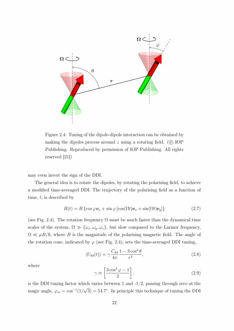
Rep. Prog. Phys. 72 (2009) 126401 T Lahaye et al
Figure 3. Tuning of the dipole–dipole interaction can be obtainedby making the dipoles precess around z using a rotating field.
where α is the angle between k and the polarization direction(see appendix A). Remarkably, in three dimensions, theFourier transform of the dipole–dipole interaction does notdepend on the modulus of the wavevector k, a feature whichis shared by the contact interaction (1.1), whose Fouriertransform is simply g.
2.2. Tuning of the dipole–dipole interaction
By using a rotating polarizing field, it is possible, by time-averaging, to tune the dipole–dipole interaction, namely toreduce its effective strength and even change its sign [41]. Fordefiniteness we consider here the case of magnetic dipoles µ ina magnetic field B(t) = Be(t) (see figure 3). The unit vectore(t) = cos ϕez +sin ϕ[cos(#t)ex +sin(#t)ey] is rotated aboutthe z-axis on a cone of aperture 2ϕ at an angular frequency #which is small compared with the Larmor frequency µB/h, butmuch larger than the trapping frequencies. Then, only the timeaverage over a period 2π/# of the dipole–dipole interaction(2.1) with e1 = e2 = e(t) plays a role in determining theproperties of the gas. This time-averaged potential reads as
〈Udd(t)〉 = Cdd
4π
1 − 3 cos2 θ
r3
[3 cos2 ϕ − 1
2
]. (2.6)
The last factor between brackets decreases from 1 to −1/2when the tilt angle ϕ varies from 0 to π/2, and vanishes whenϕ is equal to the magic angle θm. The ‘inverted’ configuration(ϕ > θm) in which the averaged dipole–dipole interaction isattractive for particles sitting side by side, allows explorationof otherwise inaccessible physics (see section 7 for someexamples of applications).
3. Creation of a dipolar gas
In order to realize a quantum gas with significant dipole–dipoleinteractions, one can use particles having either an electricdipole moment d or a magnetic dipole moment µ. Usually, thedipolar coupling is much higher in the electric case. Indeed,
Table 1. Dipolar constants for various atomic and molecularspecies. For the molecular species, the (yet unknown) scatteringlength is assumed to be 100 a0 (as the C6 coefficient of the dimer iscomparable to that of a single atom, the order of magnitude of thescattering length is similar, but obviously the actual value highlydepends on the details of the potential).
Species Dipole moment add εdd
87Rb 1.0 µB 0.7 a0 0.00752Cr 6.0 µB 16 a0 0.16KRb 0.6 D 2.0 × 10³a0 20ND3 1.5 D 3.6 × 10³ a0 36HCN 3.0 D 2.4 × 10⁴ a0 240
the typical order of magnitude of d for an atomic or molecularsystem is d ∼ qea0, where qe is the electron charge and a0
the Bohr radius, while the magnetic moments are on the orderof the Bohr magneton µB. Using the definitions of a0 and µB
in terms of fundamental constants, one sees that the ratio ofmagnetic to electric dipolar coupling constants is
µ0µ2
d2/ε0∼ α2 ∼ 10−4, (3.1)
where α & 1/137 is the fine structure constant.For a given species, it is convenient to define various
quantities to quantify the strength of the dipolar interaction.From the dipole moment (i.e. the dipolar coupling constantCdd) and the mass m of the particle, one can define thefollowing length:
add ≡ Cddm
12πh2 . (3.2)
This ‘dipolar length’ is a measure of the absolute strength of thedipole–dipole interaction. However, in some circumstances, itis the ratio
εdd ≡ add
a= Cdd
3g(3.3)
of the dipolar length to the s-wave scattering length, comparingthe relative strength of the dipolar and contact interactions,which determines the physical properties of the system. Thisdipolar parameter needs to be non-negligible if one wantsto observe dipolar effects. The numerical factors in (3.2)are chosen in such a way that for εdd ! 1 a homogeneouscondensate is unstable against 3D collapse (see section 5.1).Table 1 summarizes some typical numerical values of thedipolar constants for various atomic and molecular species.
In this section, we review the different systems that canbe used in principle to study experimentally the effect of thedipole–dipole interaction in degenerate quantum gases. Wefirst address the various candidates having an electric dipolemoment, either static or induced by a laser. The case ofmagnetic dipoles (the only system to date in which strongdipolar effects in a quantum gas have been observed) is thendescribed, with an emphasis on the experimental techniquesused to achieve Bose–Einstein condensation of chromium.
3.1. Polar molecules
Due to their strong electric dipole moment, polar molecules areideal candidates to show dipolar effects. Three requirements
5
Figure 2.4: Tuning of the dipole-dipole interaction can be obtained bymaking the dipoles precess around z using a rotating field. ( c© IOPPublishing. Reproduced by permission of IOP Publishing. All rightsreserved [21])
may even invert the sign of the DDI.The general idea is to rotate the dipoles, by rotating the polarising field, to achieve
a modified time-averaged DDI. The trajectory of the polarising field as a function oftime, t, is described by
B(t) = B cosϕez + sinϕ [cos(Ωt)ex + sin(Ωt)ey] (2.7)
(see Fig. 2.4). The rotation frequency Ω must be much faster than the dynamical timescales of the system, Ω ωx, ωy, ωz, but slow compared to the Larmor frequency,Ω µB/~, where B is the magnitude of the polarising magnetic field. The angle ofthe rotation cone, indicated by ϕ (see Fig. 2.4), sets the time-averaged DDI tuning,
〈Udd(t)〉 = γCdd
4π
1− 3 cos2 θ
r3, (2.8)
whereγ ≡
[3 cos2 ϕ− 1
2
], (2.9)
is the DDI tuning factor which varies between 1 and -1/2, passing through zero at themagic angle, ϕm = cos−1(1/
√3) = 54.7. In principle this technique of tuning the DDI
22

is also applicable for electric dipoles. From now on we incorporate the tuning factorinto the DDI, i.e. γCdd → Cdd, and it should be obvious from the context if γ 6= 1.
Tuning the DDI to zero could be useful, for example, during time-of-flight so thatthe in-situ momentum distribution can be inferred without converting DDI energy intoadditional kinetic energy. Inverted dipoles, γ < 0, open a whole new class of systemwhere the number of attractive dimensions increases to two (the radial plane) and thenumber of repulsive dimensions decreases to one (the axial direction). As a final note,it has been reported that dipolar erbium has Feshbach resonances accessible to very lowmagnetic fields [68]. This potentially makes erbium a candidate for the simultaneoustuning of both the s-wave scattering length and the DDI, since the rotation of weakfields is experimentally more feasible. However, simultaneous tuning has so far notbeen explored.
2.2 Dipolar Condensate Structure
Here we investigate the density structures of the three-dimensionally trapped dipolarBEC for various regimes and make comparisons, where appropriate, with the non-dipolar case. We begin by introducing the dipolar (and non-dipolar) Gross-Pitaevskiiequations - indispensable tools for the study of ultra-cold Bose gases. We find that thevariety of solutions for the dipolar BEC is considerably richer than for the non-dipolarcase.
2.2.1 Gross-Pitaevskii Theory
Time-Dependent Gross-Pitaevskii Equation
A powerful approach for investigating the zero temperature limit is to solve the time-dependent dipolar Gross-Pitaevskii equation DGPE [97],
i~∂ψ0(x, t)
∂t=[H0 + gsn0(x, t) + ΦD
0 (x, t)]ψ0(x, t), (2.10)
with N0 being the condensate number, n0 ≡ N0|ψ0|2 where ψ0 is the condensate wave-function normalised to unity, i.e.
∫d3x|ψ0(x)|2 = 1, and recall that H0 is the single
particle Hamiltonian. The dipole-dipole contribution to the meanfield energy is
ΦD0 (x, t) =
∫d3x′Udd(x− x′)n0(x′, t). (2.11)
Equation (2.11) is known as the direct dipolar potential which may be either: pre-dominantly negative for prolate traps where the head-to-tail attractive interactions
23

dominate; or predominantly positive for oblate trapping potentials where side-by-siderepulsive interactions are enhanced - see the schematic in Fig. 2.5.
4
uniform. In contrast, in the trapped system both direct andexchange terms contribute. To demonstrate their importance itis useful to define their individual contributions to the systemenergy as [see Eq. (9)]
ED =1
2
∫dxdk
(2π)3ΦD(x)W (x,k), (13)
EE = −1
2
∫dxdk
(2π)3ΦE(x,k)W (x,k), (14)
which we shall refer to as the direct and exchange energies,respectively.
T/T 0F
ED/N
hω,E
E/N
hω
0 0.2 0.4 0.6 0.8 1-8
-6
-4
-2
0
2
4
6
8
FIG. 2. (Color online) Direct and exchange energy versus tempera-ture for a dipolar Fermi gas. Direct energy ED (solid) and exchangeenergy EE (dashed). Aspect ratios λ = 0.1 (blue/dark grey lines), 1(green/light grey lines) and 10 (red/grey lines). Interaction parameterDt = 1. Note that the ED and EE results for the λ = 1 case arealmost indistinguishable.
FIG. 3. (Color online) Schematic showing how the distribution ofdipoles in (a) prolate, (b) spherical, and (c) oblate geometries.
We present results for these energies in Fig 2. We ob-serve that the direct interaction energy is strongly effected bythe trap geometry, is significantly increased in magnitude inhighly anisotropic traps and can be both positive and nega-tive. The exchange interaction energy is only slightly affected
by the trap geometry and is always negative. Except for nearlyspherical traps, the magnitude ofEE tends to be much smallerthan ED .To explain these observations we begin by considering the
direct energy. The sign and strength of this quantity is con-trolled by the trap geometry, through its influence on the sys-tem spatial density profile: A prolate spatial density causesthe attractive component of Udd (i.e. interactions with dipolesin a head-to-tail configuration, see Fig. 3(a)) to dominate andED is negative, and increasing in magnitude as the systembecomes more prolate. An oblate spatial density causes therepulsive component of Udd (i.e. interactions with dipoles in aside-by-side configuration, see Fig. 3(c)) to dominate and ED
is positive, and increasing as the system becomes more oblate.Note that the spatial density profile has a geometry that is usu-ally close to the trap aspect ratio λ, however interactions causeadditional distortion (as has already characterized by the pa-rameter β). For example, in the spherical trap interactions willcause the spatial density to deform to be slightly prolate andED will be slightly negative, as we see in Fig 2.A rather similar geometric argument can be applied to the
exchange interaction, but now for the momentum space dis-tribution: It is energetically favorable for the momentum dis-tribution to compress along kρ and expand along kz . Interest-ingly for bosons, where the negative sign does not accompanythe exchange term, the opposite momentum behavior wouldbe expected. However, any anisotropy in the momentum den-sity arises solely from the dipole interaction itself in all caseswe consider1 and |EE | tends to be much smaller than |ED|,except in nearly spherical traps.
3. Chemical potential
We present results for the low temperature chemical poten-tial of the trapped dipolar gas in Table I for the main systemparameters considered in this paper. We consider the ratioµ/kBT 0
F , which gives us a quantitative measure of the effectof interactions on the Fermi temperature of the interacting sys-tem. In practice we evaluate these results at the small but finitetemperature of T = 0.01T 0
F . We do this because the lowesttemperature we can solve for is limited by the ability of thecomputational grids we use to resolve the sharp Fermi surface.However, as shown in Fig. 4, the chemical rapidly saturates asT → 0 and the values calculated at T = 0.01T 0
F should bevery close to the T = 0 value.The behavior of the chemical potential has been considered
for the uniform gas in [29]. In that work it was found that in-creasing the dipolar interaction strength suppressed µ. In thetrapped system we observe that prolate trapping geometry canenhance this suppression, while an oblate geometry can in-
1 The isotropy of mass ensures the non-interacting momentum distributionis isotropic, however this could be changed, e.g. by using an optical latticeto modify the effective mass in different directions. It may be possible toextend our meanfield analysis to this case, e.g. see [35].
Figure 2.5: Schematic showing the distribution of dipoles in (a) pro-late, (b) spherical and (c) oblate geometries. (Copyright (2010) byThe American Physical Society [98])
Time-Independent Gross-Pitaevskii Equation
For equilibrium stationary solutions of the form ψ0(x, t) = ψ0(x)e−iµt/~ the time de-pendence may be eliminated from Eq. (2.10) giving the time-independent DGPE,
µψ0(x) =[H0 + gsn0(x) + ΦD
0 (x)]ψ0(x), (2.12)
where µ is the chemical potential.
Gross-Pitaevskii Energy Functional
Equivalent to finding stationary solutions of time-independent DGPE, is to minimisethe Gross-Pitaevskii (GP) energy functional,
E[ψ0] =
∫d3xψ∗0(x)
[H0 +
gsn0(x)
2+
ΦD0 (x)
2
]ψ0(x), (2.13)
A common method for finding GP ground states is by propagating an initial state,according to the DGPE (Eq. (2.10)), in imaginary time 3. However, this method isslow and the Bohn group [99], for example, instead employ a scheme that directlyminimises the GP energy functional (Eq. (2.13)) using a conjugate-gradient technique.
3This is also a common method for solving the non-dipolar GPE (Eq. (2.14))
24

The general idea of conjugate-gradient methods is to minimise the energy functional by"successive line minimisations along optimally chosen directions" [100]. This methodis significantly more efficient than simply taking the path of steepest descent.
2.2.2 Thomas-Fermi Regime
Contact Interaction
The (non-dipolar) Gross-Pitaevskii equation (GPE) was derived independently in 1961by Gross [101, 102] and Pitaevskii [103, 104] and has since become a well-establishedtool for investigating BECs. The non-dipolar GPE is trivially related to the DGPE,e.g. the time independent version takes the form (cf. Eq. (2.12))
µψ0(x) =
(−~2∇2
2m+ Vtrap(x) + gsn0(x)
)ψ0(x). (2.14)
For large N0 the interaction energy may dominate the kinetic energy over much of thecondensate, i.e.
gsn0(x)ψ0 ∣∣∣∣~2∇2
2mψ0
∣∣∣∣ , (2.15)
and a reasonable approximation is to neglect the kinetic energy altogether. This isknown as the Thomas-Fermi approximation and has the analytic solution
n0(x) =
[µ− Vtrap(x)]/gs , µ > Vtrap,
0 , otherwise.(2.16)
For the case of harmonic confinement,
Vtrap =m
2(ω2
xx2 + ω2
yy2 + ω2
zz2), (2.17)
the solution takes the form of a 3D inverted parabola with the width in each direc-tion independently set by the corresponding trap frequency. The density profile ofEq. (2.16) broadens as the repulsive interaction strength gs increases and, in general, isconsiderably wider than the limit of a non-interacting condensate (harmonic oscillatorground state),
nNI0 (x) = N0
(mωπ~
)3/2
exp[−m
~(ωxx
2 + ωyy2 + ωzz
2], (2.18)
with ω ≡ (ωxωyωz)1/3 being the geometric mean trap frequency.
25

Dipolar Interaction
The dipole-dipole interaction is long-ranged and anisotropic so it is perhaps intuitivelyunclear as to what shape the Thomas-Fermi ground state may take. Surprisingly, arather involved derivation by O’Dell et al. [105, 106] shows that the dipolar Thomas-Fermi solution also has inverse parabolic form,
n0(x) =15N0
8πRxRyRz
[1− x2
R2x
− y2
R2y
− z2
R2z
], (2.19)
but with an aspect ratio distorted by magnetostriction (or electrostriction).Here we outline their result and demonstrate how to calculate the widths for the
cylindrically symmetric case, ωx = ωy ≡ ωρ and Rx = Ry ≡ Rρ, although this is not anecessary restriction. Defining the condensate aspect ratio κ ≡ Rρ/Rz and trap aspectratio λ ≡ ωz/ωρ, the radial width takes the form,
Rρ =
[15gN0κ
4πmω2ρ
1 + εdd
(3
2
κ2f(κ)
1− κ2− 1
)]1/5
, (2.20)
where,
f(κ) =1 + 2κ2
1− κ2− 3κ2arctanh
√1− κ2
(1− κ2)3/2(2.21)
(recall that εdd is defined by Eq. (1.8)). Unlike the non-dipolar case, the value of κdepends on the DDI strength (through εdd) and is obtained by numerically solving thetranscendental equation,
κ2
λ2
[3εddf(κ)
1− κ2
(λ2
2+ 1
)− 2εdd − 1
]= εdd − 1. (2.22)
2.2.3 Exotic Ground States
Theoretical works have found that for dipolar condensates the Thomas-Fermi approx-imation is often inappropriate. As will be discussed in Sec. 2.4 - if the DDI becomestoo large then the system will become unstable and collapse to a dense state, thus forstable systems the kinetic energy remains an important consideration. A more realisticapproach is to solve the full DGPE which we outlined in Sec. 2.2.1. Several groupshave solved these equations in various regimes and here we briefly review some of thefindings.
Blood Cell
Interestingly, the Bohn group found that for certain regimes with cylindrical symme-try the ground state density resembles a red blood cell, with the maximum density
26

i@ @ !r; t"@t
#!$ @2
2Mr2 %M!2
!
2!!2 % "2z2"
% !N $ 1" 4#@2a
Mj !r; t"j2 % !N $ 1"
&Zdr0Vd!r$ r0"j !r0; t"j2
" !r; t"; (1)
where M is the particle mass and the wave function isnormalized to unit norm. The coupling constant for theshort-range interaction is proportional to the scatteringlength a, although we set a # 0 in the following. Thedipole-dipole interaction is given by Vd!r" # d2!1$3cos2$"=r3, with $ being the angle between the vector rand the z axis. We also define a dimensionless dipolarinteraction parameter, D # !N $ 1"Md2=!@2aho", where
aho #################@=M!!
qdenotes the transverse harmonic oscillator
length. It is convenient to think of increasing D as equiva-lent to increasing the number of dipoles.
A stable condensate exists when there is a stationarysolution of Eq. (1) which is stable to small perturbations.Based on this criterion, we have constructed the stabilitydiagram in Fig. 1, as a function of D and the trap aspectratio " # !z=!!. In the figure, the shaded and white areasdenote parameter ranges for which the condensate is stableor unstable, respectively. In general, the more pancakelikethe trap becomes (larger "), the more dipoles are requiredto make the condensate unstable. But eventually, the con-densate always becomes unstable for a large enough num-ber of particles. This result is at odds with the conclusion ofRef. [4], but in agreement with that of [5,17]. The reasonfor the different conclusion of Ref. [4] is not clear, but wefind that the for highly pancake traps, a larger grid size, andsignificantly larger computation time are required toachieve convergence. Moreover, our numerical calcula-tions were facilitated by our new algorithm [15], but wechecked that we got the same results using the numericalmethods of Ref. [4], provided that we used a large enoughgrid and strict convergence criterion.
Remarkably, there appear regions in parameter spacewhere the condensate obtains its maximum density awayfrom the center of the trap. These are the darker shadedareas in Fig. 1. The local minimum of the density in thecenter gives the condensate a biconcave shape, resemblingthat of a red blood cell (a surface of constant density isillustrated at the top left corner of Fig. 1). A densitycontour plot of such biconcave condensate is shown inFig. 2(IIa), with the parameters " # 7 and D # 30:8.These structures appear in isolated regions of the parame-ter space, and, in particular, only for certain aspects ratiosin the vicinity of " ' 7; 11; 15; 19 . . . . There seems to be arepeated pattern which probably continues to larger valuesof " (although this was not calculated). However, theparameter space area of these regions becomes increas-ingly small with larger ", and is already negligible for the
fourth region (not shown in Fig. 1). In between the bicon-cave regions, we find ‘‘normal’’ condensates with maxi-mum density in the center, Fig. 2(Ia). Their density profilesin fact have a fairly sharp peak in the center, as comparedto a Gaussian shape.
To verify the existence of biconcave structures, we solveEq. (1) numerically both with a 3D algorithm [7] and withour 2D algorithm that exploits the cylindrical symmetry[15], carefully converging both the grid size and resolution.We have also carried out a variational calculation, in whichthe condensate wave function is taken to be a linear com-bination of two harmonic oscillator wave functions. Thefirst is a simple Gaussian, and the second is the sameGaussian multiplied by [H2!x" %H2!y"], where H2 is theHermite polynomial of order 2, and (x, y) are the coordi-nates perpendicular to the trap axis. Minimizing the varia-tional energy, we find biconcave solutions with a largecomponent of the second wave function, similar in shapeto the numerical ones. The exact parameters for appearanceof variational biconcave condensates are somewhat differ-ent from the numerical ones, and the variational calculationgives a continuous parameter region with biconcave con-densates, rather than isolated regions as we find numeri-cally. This is probably due to the oversimplified nature ofthe variational ansatz.
We find that the existence of islands of biconcave con-densates is robust to the addition of small contact interac-tion, with scattering length a up to (20% of the dipolar
FIG. 1 (color online). Stability diagram of a dipolar conden-sate in a trap, as a function of the trap aspect ratio " # !z=!!
and the dipolar interaction parameter D. Shadowed areas arestable, while white unstable against collapse. In the darker,isolated areas, we find biconcave condensates (illustrated withisodensity surface plot at the top right corner) whose maximaldensity is not at the center. The contours in the biconcave regionsindicate the ratio of the central density to the maximal density,with darker areas having a smaller ratio. The contour intervalsare 10%, and the minimum ratio obtained is 70%.
PRL 98, 030406 (2007) P H Y S I C A L R E V I E W L E T T E R S week ending19 JANUARY 2007
030406-2
Figure 2.6: Isodensity surface of the ground state solution in a cylin-drically symmetric trap with aspect ratio λ ≈ 8. The polarising fieldis aligned along the tight axis of the trap. (Copyright (2007) by TheAmerican Physical Society [99])
occurring on a ring in the radial plane, as demonstrated by the isodensity surface inFig. 2.6. The polarising field is aligned along the pancake trap’s tight direction and,by ‘pushing’ the region of high density radially outward, the peak density and therepulsive side-by-side DDIs are reduced.
Multi-Peaked Structures
In general, exotic solutions that do not have a centrally positioned peak are knownas ‘density-oscillating ground states’. Both Refs. [108] and [107] investigated how theblood cell shape changes by breaking cylindrical symmetry, i.e. allowing all three trapfrequencies to be varied independently. Reference [108] solves the DGPE (Eq. (2.10))using the usual ‘imaginary time evolution’ method. Alternatively, Ref. [107] directlyminimises the GP energy functional (Eq. (2.13)) using a method similar to that usedby Ref. [100], but implementing the Newton-Krylov instead of the conjugate-gradientminimisation routine. Figure 2.7 characterises the various kinds of density-oscillatingground states found, including ‘simple two-peaked’, ‘two-peaked separated by a crater’and ‘four-peaked’ solutions.
Dumbell
Reference [109] investigated ground state solutions with inverted dipoles, i.e. γ < 0 inEq. (2.8). The numerical method implemented was the usual ’imaginary time evolution’of the DGPE (Eq. (2.10)). Notably, their results showed that for cigar shaped traps theground state density acquires a dumbbell-shaped form in certain parameter regimes, forexample see Fig. 2.8. Recall that negative dipoles aligned head-to-tail repel each other,
27

STABILITY AND STRUCTURE OF AN ANISOTROPICALLY . . . PHYSICAL REVIEW A 86, 053623 (2012)
(a)
(b)
I
II
III
IV
V
I
II
III
IV
(c)
(d)
I
V
III
II IVIII
II
(e)
D
D D
D D
λx
λz
λx λx
λx λx
I
III
IIIV
V
λx
λz
(f) (g)
λx
λz
I
II
FIG. 1. (Color online) (a) Stability plot of a dipolar condensatein an anisotropic trap as a function of the anisotropy parameters λx
and λz and dipole strength D. In the dark-shaded (magenta) regionthere exist stable density-oscillating condensates (with the maximumdensity away from the center of the condensate). The light-shaded(cyan) regions are normal ground states with maximum density attrap center. The slice in the λz direction, corresponding to cylindricalsymmetry λx = 1, is displaced from the axes to improve visibilityand reproduces Fig. 1 of Ref. [24]. (b)–(e) Stability plots for constantλz = 6 (b), 6.5 (c), 7 (d), and 8 (e) with the type of state labeled I–Vaccording to the classification given in Sec. III B. (f) and (g) Stabilityplots for constant D = 15 (f) and 30 (g).
can be understood because the DDI is attractive for dipoles ina head-to-tail configuration (z separation) and repulsive fordipoles in a side-by-side configuration (xy-plane separation).Thus increasing λz (tightening z confinement) reduces thenumber of dipoles in the destabilizing attractive configuration,while decreasing λx (loosening x confinement) increases thenumber of dipoles in the stabilizing repulsive configuration.
I II
(b)
(a)
II III
IV V
x/lyy/ly
FIG. 2. Different types of ground-state density profiles. Densityslice of the condensate in the xy plane, focusing on the central regionwhere density oscillations can occur. Solutions give examples of thevarious condensate types (I–V) and are obtained for the parameters I(λx,λz,D) = (0.65,9,89.4), II(a) (0.85,6,20.3), II(b) (0.9,6.5,26.3),III (0.6,6.5,50.1), IV (0.65,6,37.8), and V (1,6.5,24). See text inSec. III B for a discussion of the ground-state types.
B. Ground-state types
We find that a density-oscillating condensate can exhibit arange of different shapes; however, in the region of interest thez confinement is sufficiently tight that the nontrivial densityfeatures occur in the xy plane. Following [40], we categorizethe ground-state solutions by the labels I–V as follows, withreference to examples in Fig. 2.
Type I. Normal (non-density-oscillating) condensate withpeak density at the origin.
Type II. Density-oscillating condensate with two peaksin the x direction. This can either be a simple two-peakedstructure [e.g., Fig. 2 II(a)], or two peaks with a biconcavecrater [e.g., Fig. 2 II(b)].
Type III. Density-oscillating condensate with two peaksin the y direction. Like type II, this case could be a simpletwo-peaked case (not shown) or with a biconcave crater.
Type IV. Density-oscillating condensate with four peaks(two peaks along both the x and y directions).
Type V. Density-oscillating condensate that is biconcave(with no additional peaks).
In Fig. 3(g), we present a projection (bird’s-eye view) ofthe stability diagram [Fig. 1(a)] onto the λxλz plane, indicatingthe different types of ground states which occur. Normal(type-I) condensates are found in the light shaded regionfor any value of D. Dark shaded regions indicate if a stabledensity-oscillating state exists for any value of D in that trapgeometry. The darkly shaded region is subdivided according tothe type of density-oscillating state (types II–V) at the largestdipole strength D for which a stable ground state exists at thatvalue of λx , λz.
053623-3
Figure 2.7: Different types of ground-state density profiles. Den-sity slices of the condensate in the xy plane, focusing on the centralregion where density oscillations occur. Solutions give examples ofthe various condensate types and are obtained for the parameters I(ωx/ωy, ωz/ωy, CddNm/4π~2ly) = (0.65, 9, 89.4), II(a) (0.85, 6, 20.3),II(b) (0.9, 6.5, 26.3), III (0.6, 6.5, 50.1), IV (0.65, 6, 37.8), and V (1,6.5, 24), where ly =
√~/mωy. (Copyright (2012) by The American
Physical Society [107])
28

so the axial separation of the two high density clumps acts to decrease the interactionenergy.
SPATIAL DENSITY OSCILLATIONS IN TRAPPED . . . PHYSICAL REVIEW A 82, 023622 (2010)
FIG. 6. (Color online) Contact interaction strength dependenceof the upper critical dipolar interaction D
(−)λ for a condensate in
cigar-shaped traps. The shaded areas mark the DOIs. The inset showsthe typical result for the isodensity surface of the condensate. Thebroken arrows denote the direction to which the DOIs move as λ isdecreased.
the contact interaction strength. Again, the energies are smoothfunctions of g across the boundary of a DOI.
The stability diagram of a dipolar condensate in cigar-shaped traps is presented in Fig. 6 where the DOIs appear whenλ ! 0.3.In contrast to the D > 0 case, the dipolar interactionbecomes repulsive (attractive) along the axial (radial) directionfor D < 0. Therefore, along the z direction, the repulsivedipolar force depletes the density at the center of the trapsuch that the isodensity surface of the condensate with SDOtakes a dumbbell-shaped form. By corresponding to dumbbellstructure, the effective potential [Fig. 3(b)] takes the form of adouble-well potential. As the trapping potential becomes morepancake shaped, the DOIs move along the stability boundaryto the negative direction of the g axis; in addition, the area ofthe DOI shrinks.
We remark that our results do not rule out the possibilitythat more DOIs might exist for larger g values, since ournumerical calculations have only covered limited ranges ofthe parameters λ and g.
B. Free expansion
Now, we turn to study the expansion of initially trappeddipolar condensates. Compared to the contact interaction,the anisotropic nature of the dipolar interaction makes theexpanded cloud behave quite differently [26–28]. Indeed, ithas been used experimentally as a diagnostic tool for detectionof the dipolar effects in Bose-Einstein condensates [4,8,9].
To study the free expansion dynamics, we consider aninitially trapped condensate with control parameters (λ,g,D),which falls into a DOI. At time t = 0, we switch off thetrapping potential; the expansion dynamics of the condensateis then described by Eq. (2) with Uho = 0. If the interactionsare ignored completely during expansion, the condensate willexpand ballistically such that the time-of-flight image repre-sents the momentum distribution of the trapped condensate.From the Fourier transform of the initial wave function withSDO, one can easily deduce that two side peaks would appearin the time-of-flight image, which can be used as the signatureof the oscillating density profile in the initial condensate.
To demonstrate this, we consider the expansion of aninitially cigar-shaped condensate obtained by using the controlparameter (λ,g,D) = (0.2,35,−18). Here, instead of tuning
(a)
x(a⊥)
z(a
⊥)
(c)
−20 −10 0 10 20−15
0
15
(b)
(d)
FIG. 7. (Color online) Column density of the expanded cloud for(a) ω⊥t = 0, (b) 3, (c) 5, and (d) 8. The initial states are obtained byusing (λ,g,D) = (0.2,35,−18); during the expansion, g is tuned tozero.
both g and D to zero, we only switch off the contact interactionfor t > 0. Figure 7 shows the column densities of the expandedcloud, that is,
n(x,z,t) =∫
dy n(x,y,z,t). (8)
Due to the dumbbell-shaped density profile, the initial columndensity has two peaks analogous to that of the condensatetrapped in a double-well potential. After the condensateexpands such that these two peaks overlap, the third peakappears as a result of the interference. At time ω⊥t = 5, threepeaks have roughly the same height. When the system evolvescontinuously, the heights of the two side peaks become lowerand lower, but they are still visible at ω⊥t = 8. However, if thecontact interaction remains unchanged during free expansion,the preceding scenario will be spoiled such that the side peakswill vanish very quickly for a cigar-shaped condensate.
Fortunately, for a pancake-shaped condensate, the sidepeaks of the column density remain visible for a long timeif, initially, the dipolar interaction is very close to the stabilityboundary. In Fig. 8, we demonstrate the free expansion of apancake-shaped condensate with an initial wave function ob-tained by using the control parameters (λ,g,D) = (7,−5,33).To make it easier to visualize the structure of the expandedcloud, we also plot the column density on the x axis. Itcan be seen that, even for ω⊥t = 7, the side peaks are stilldistinguishable from the column density, which indicates thatthe time-of-flight image may be used to detect the SDO in adipolar condensate.
V. DIPOLAR CONDENSATE IN A BOX POTENTIAL
In this section, we briefly discuss the SDOs of a dipolarcondensate trapped in a box potential. Specifically, we considera potential that is harmonic along the z axis with frequency ωz
but is represented by infinite square wells with length L alongthe x and y axes. Such potential can be realized by using, forexample, a tightly focused light sheet [29].
Figure 9 displays the stability diagram of such a system.As in the previous case, a critical dipolar interaction strength
023622-5
Figure 2.8: Isodensity surface of the ground state solution in a cylin-drically symmetric cigar shaped trap, λ = 0.3. (Copyright (2010) byThe American Physical Society [109])
Finally, as a general comment on the various kinds of exotic ground states (alsotermed density oscillating ground states), we note that these occur when the DDIbecome large. In fact, they occur within islands of parameter space that border theinstability region termed density oscillation islands (DOIs). For more details about therelationship between density oscillating ground states and instability see Sec. 2.4.3.
2.3 Elementary Excitations
2.3.1 The Quasi-2D Uniform System
As we shall see in Sec. 2.4.2, the purely dipolar BEC is always unstable in the 3Duntrapped regime. Stability may be attained however, by introducing a confiningpotential along the polarisation direction that acts to limit the head-to-tail attractionbetween dipoles. Here we consider the simple case of a quasi-2D uniform system (seeFig. 2.9), unconfined in two dimensions but harmonically confined in the direction ofpolarisation. Crucially however, the confinement is loose enough such that the atomsare free to move and interact in 3D 4.
4Roughly speaking this requires the z-confinement length to satisfy az as, add, a conditionnormally well satisfied in experiments.
29

−4
−3
−2
−1
0
1
2
3
4
00.2
0.4
0.6
0.8 1
1.2
1.4
1.6
1.8
Figure 2.9: In-plane cross sectional view of the quasi-2D system.The gas is harmonically trapped in the direction of polarisation (z-direction), where we assume the density to take a gaussian form, anduntrapped in the x-y plane perpendicular to polarisation.
Following Ref. [110] (also see [111]) we assume a gaussian profile for the BECdensity along the confined direction, which we will refer to as the gaussian ansatz 5.Let us begin with an important result dating back to the 1940s, namely the Bogoliubovdispersion relation for the homogeneous BEC [114],
E(k) =
√~2k2
2m
~2k2
2m+ 2n0U(k)
, (2.23)
where U(k) is the Fourier transform (FT) of the interparticle interaction potential andn0 is the density.
Using the gaussian ansatz, the z-direction of the problem can be analytically inte-grated - we are therefore interested in the quasi-2D interaction potential,
U q2D(ρ) ≡ U q2D(ρ1 − ρ2) =
∫ ∫dz1dz2χ(z1)χ(z2)U(x1 − x2), (2.24)
where for the first step we made use of the translational invariance within the planedefined by ρ ≡ x, y. Note that
χ(z) =1
az√π
exp
[−z
2
a2z
], (2.25)
is the density profile in the z-direction, normalised to one, and az =√
~/mωz is theharmonic oscillator confinement length.
5Note that Ref. [112] assumes an inverted parabola density profile along the confinement direction.Reference [113] shows that results for the radially trapped system are quantitatively sensitive to theprecise density ansatz in the z-direction but are qualitatively indifferent (also see Fig.2.22). To ourknowledge, such comparisons have not been made for the quasi-2D uniform system.
30

Substituting the full interaction potential (Eq. (1.6)) into Eq. (2.24) and taking theFT of U q2D(ρ) gives [110]
U q2D(kρ) =1
az√
2π
(gs + gddF⊥
[kρaz√
2
])(2.26)
where gdd ≡ 4π~2add/m, gs ≡ 4π~2as/m and
F⊥(Q) = 2− 3√πQeQ
2
erfc(Q), (2.27)
with erfc(Q) being the complimentary error function. In Fig. 2.10 we plot F⊥ whichexhibits a strong momentum dependence and has the following asymptotic properties:
F⊥(Q→ 0) = 2, (2.28)
and F⊥(Q→∞) = −1. (2.29)
0 1 2 3 4-1
0
1
2
kρaz/√
2
F⊥
(kρa
z/√
2)
Figure 2.10: Plot of Eq. (2.27) showing the momentum dependenceof the quasi-2D DDI.
Inserting the quasi-2D interaction energy into Eq. (2.23) gives the quasi-2D disper-sion relation,
E(kρ) =
√√√√~2k2ρ
2m
~2k2
ρ
2m+n2D
√2
az√π
(gs + gddF⊥
[kρaz√
2
]), (2.30)
with the average areal density, n2D =∫dzn(x), which is spatially invariant in the
uniform system.
31

2.3.2 Phonons and Free Particles
Consider two limits of Eq. (2.30), the first being the small momentum limit kρaz → 0,which using Eq. (2.28) we obtain
E(kρ → 0) = ~kρ√
n2D
maz√
2π(gs + 2gdd), (2.31)
resulting in a linear dispersion relation. Such a dispersion relation is said to be phononicand may be characterised by its speed of sound,
c =
√n2D
maz√
2π(gs + 2gdd). (2.32)
In the alternative limit of large momentum, kρaz → ∞, F⊥ remains finite (seeEq. 2.29) and we obtain the free particle dispersion relation
E(kρ →∞) =~2k2
ρ
2m, (2.33)
with the effects of interactions being negligible.In Fig. 2.11 we plot the Bogoliubov dispersion relation for a BEC interacting only
via the contact interaction. For comparison, the phonon and free particle limits arealso shown.
2.3.3 Rotons and Maxons
Liquid Helium
Revolutionary work in the 1940s by Landau, on the theory of superfluidity of liquid4He, brought forward the idea of phonons and rotons as elementary excitations ofthe superfluid phase. He proposed that rotons would form a local minimum of thedispersion relation E = ∆+~2(k−k0)2/2µ, where ∆ is the height of the local minimum,k0 is the average roton wavenumber and µ is a constant determining the curvature. In1954 Feynman derived a relationship between the dispersion relation and the staticstructure factor, E = ~2k2/2mS(k) [115]. He then used measurements of the staticstructure factor from neutron diffraction experiments to support Landau’s predictionof a rotonic local minimum of the dispersion relation. This result, shown in Fig. 2.12,shows that a bump of the static structure factor is associated with a roton minimum ofthe dispersion relation. Although rotons originally got their name due to their predictedmanifestation as vortices, experiments have not confirmed whether this is necessarilythe case. The excitations at the local maximum, prior to the roton minimum, of the
32

0 0.5 1 1.5 20
0.5
1
1.5
2
2.5
kρ
E(k
ρ)
E = c hkρ
E =h2k2
ρ
2m
Figure 2.11: Bogoliubov dispersion relation, Eq. (2.30), for a quasi-2D BEC interacting only via contact interactions, i.e. gdd = 0. Thephonon limit, characterised by the speed of sound c, and the freeparticle limit are plotted as red and cyan dashed curves respectively.For illustration purposes we set ~ = m = n2D = az = gs = 1.
dispersion relation are known as maxons and together these constitute the roton-maxondispersion relation.
Pure 2D Dipolar Gas
It has been predicted that an analogous roton spectrum may exist for pure 2D dipolarcondensates. The pure 2D regime is obtained by confining an ultra-cold gas in thez-direction so tightly that particles can only approach and interact with each otherside-by-side, i.e. head-to-tail interactions are completely supressed. In such a limit thefull DDI (see Eq. (1.2)) reduces to the 2D version, which is purely repulsive,
U2Ddd (ρ) =
Cdd
4πρ3. (2.34)
33

Figure 2.12: The upper curvegives the static structure factordetermined from neutron diffrac-tion and extrapolated to zero k.The lower curve gives the en-ergy spectrum of excitations as afunction of wave number whichresults from the formula E =
~2k2/2mS(k). The initial linearportion represents excitations ofphonons while excitations near theminimum of the curve, where itbehaves as ∆+~2(k−k0)2/2µ, cor-respond to Landau’s rotons. How-ever, data on specific heat indicatethe theoretical curve should lielower, closer to the dashed curve.(Copyright (1954) by The Ameri-can Physical Society [115])
ATOMI C THEORY OF 2 —FLUI D MODEL OF LIQUID He 267
so a few remarks might be appropriate here. It looksat 6rst, on inspection of the 6rst factor, that this repre-sents the excitation of a single particle. This is correctat very high k(ka))2s. ) and it is also correct for theideal gas case for which the atoms do not interact(@ is constant then). But our arguments for inter-mediate k show that this is not the case. Because of thecorrelations in position implied by the factor p, themotion of one atom implies the motion of others. Thusthe factor in front of p selects from that function certaincorrelated motions, in spite of the fact that each termin the factor depends on just one variable.We can get a better idea of how this works by taking
the extreme case of very low k. Here (22) represents asound wave but at first sight there is no sign of thedensity variations that such a wave usually brings tomind. Let us take the real part and consider
P; cos(k r~)p (23)
for small k. Now, for most configurations, allowed by @,the atoms are fairly uniformly distributed, so thatthere are just as many in the regions where the cosineis positive, as where it is negative. Therefore the sumover all the atoms of cos(k r;) is zero. The wave func-tion is zero for nearly all con6gurations. It is only forthe rare configurations in which the number in positiveregions exceeds that in regions where the cosine isnegative that the wave function does not vanish. In thisway (23) selects configurations for which the meandensity varies as cos(k r). Since such density fluctua-tions are, according to the behavior of P, most likelyproduced by small cooperative motions of large numbers
Although we have made an argument only to showthat (2) should be valid for high k, we see now that itis also valid. for small k, that is for f(r) which varyslowly. Since the energy curve is valid for the smaller kand for a range about 2w/a, we can accept it as reason-able for all k from zero up to and slightly beyond theminimum.On the other hand, for still larger k, another state of
lower energy exists with the same total momentum.It is the state of double excitation, one of kr, the otherof ks, such that kr+ks ——k and still E(kr)+E(ks) (E(k).This becomes possible for k so high that the slope dE/dkof the energy curve exceeds Ac, the initial slope. Thecurve for very large k, therefore, does not have the samevalidity as that for lower k, but we need not enter intothis matter, because at temperatures of a few degreessuch high-energy states would not be appreciablyexcited. Such questions may be of importance in dis-cussing nonequilibrium phenomena. One process bywhich the number of excitations can change is for anexcitation to pick up enough momentum that it candivide spontaneously into two.It is easy to misinterpret the meaning of the wave
function(2-')
&.0$(K)
0.5
00
Ok )0-zOJ
EOi~ 5-hlXI
W
lD 20 30 A l
WAVE NUMBER K
0 l0 2Q 504 ~
NAVE NUMBER K
+IG. 3. The upper curve gives the liquid structure factor deter-mined from neutron diIIraction (reference 5) and extrapolated tozero k. The lower curve gives the energy spectrum nf excitations asa function of wave number (momentum k ') which results fromthe formula 8=k'ks/2rsS(k) derived in the text. The initial linearportion represents excitation of phonons while excitations nearthe minimum of the curve, where it behaves as 6+5'(k—ko)'/2p,correspond to Landau's rotons. However, data on the speci6c heatindicate that the theoretical curve should lie lower, closer to thedashed curve.
of atoms, the state described is very far from the oneparticle state it would be if the cosine factor appearedalone, not multiplied by P.In the region of the energy minimum at ko the wave
function represents a situation intermediate betweenthe cooperative motion of phonons, and the excitationof a single particle. Several atoms move together be-cause of the correlations implied by P. It is hard to makea clear picture out of this vague idea. There is nothingto indicate that the state carries an intrinsic angularmomentum. One must be careful because the state isdegenerate, as all directions of k with the same magni-tude ko give the same energy A. Perhaps, if more com-plicated wave functions were tried, some special linearcombination representing a kind of microscopic vortexring or one with intrinsic angular momentum has in facta lower energy. States of low k will be called phonons,and states of momentum near ko will be called rotons inthis paper, in accordance with the terminology ofLandau, ' although we do not necessarily mean to implythat rotons carry intrinsic angular momentum or repre-sent vortex motion.
MULTIPLE EXCITATION
We have obtained the energy spectrum E(k) of whatwe may call single excitations. They have the form of' L. Landau, J. Phys. U.S.S.R. S, 71 (1941); 8, 1 (1941). See
also R. B.Dingle, Supplement to Phil. Mag. I, 112 (1952).
In Fig. 2.13, Filinov et al. calculate rotonic dispersion relations using path integralMonte Carlo simulations [116]. As the DDI strength (represented by D in their termi-nology) increases a roton minimum develops and deepens.
The origin of this pure 2D dipolar roton, as well as the liquid helium roton, is dueto the quasi-localisation of the (correlations between) particles which are separated bystrong repulsive interactions. A requirement for such systems is high density and stronginteractions in order to reach the strongly correlated regime. If the DDI becomes sostrong that the roton minimum touches zero energy (referred to as going soft) then thesystem transitions to 2D crystalline phase with triangular structure [18, 28, 29].
Weakly Interacting Dipolar Gas
After considering the physical mechanism behind the strongly interacting rotonic sys-tems of liquid He and the purely 2D dipolar case, one would be forgiven for discountingthe possibility of such intriguing excitation spectra for dilute weakly interacting BECs.It may have came as some surprise then that, in 2003, Santos et al. [112] made the
34

generalized to finite temperatures:
!ðqÞ # !FðqÞ; !FðqÞ tanh!@!FðqÞ
2T
"¼ @q2
2mSðq; TÞ ;
(4)
where Sðq; TÞ is the static structure factor. The latter wascomputed below and above Tc: 0:5# T # 3:3; cf. Fig. 3(a).As D approaches the crystallization point, a sharp peakdevelops near the wave number q0 corresponding to themean interparticle distance q0a ¼ 2!. While Sðq; TÞshows some T dependence for qa < 3, !Fðq; TÞ stays al-most unchanged in a broad temperature interval T & 3:3and is close to the ground-state result [7,20]. Therefore, thespectra shown in Fig. 4 for T ¼ 0:5 are representative forthe low-temperature behavior.
In the long wavelength limit qa ! 0, !F yields a lineardispersion: !FðqÞ ¼ cq; cf. Fig. 4(a), which is in agree-ment with the result for classical 2D dipoles [21,22]. Ourresults for the sound speed, cðTÞ ¼ !Fðq; TÞ=qjq!0, ex-tracted from the data for N ¼ 324 particles are summa-rized in Table I and agree within 4% with the ground-statevalues of Ref. [7].
A significant improvement of the spectrum is achievedby using a sum-rule approach [23,24] by combining thePIMC results for Sðq; TÞ and the static density responsefunction "ðq; TÞ. This yields a rigorous upper bound@!ðqÞ # @!"ðq; TÞ ¼ 2nSðq; TÞ="ðq; TÞ;
"ðqÞ ¼ %Z #
0Fðq; $Þd$; Fðq; $Þ ¼ 1
Nh%qð$Þ%qð0Þi;
(5)
where "ðqÞ is obtained from the imaginary-time density-density correlation function Fðq; $Þ directly evaluated inour PIMC simulations. With the increase of D, "ðqÞsharpens and its peak shifts continuously towards q0; cf.Fig. 3(b).
In Fig. 4, we show !" [Eq. (5)] together with theFeynman spectrum and the correlated basis functions(CBF) result [25] at four dipole couplings. All three ap-proximations show the same general trend which resem-
bles superfluid helium: With increasing coupling thespectrum develops a roton minimum at finite q & q0 whichbecomes deeper with increasing D. While for qa & 1:5(sound range) all approaches are in quantitative agreement,for qa > 2 the Feynman approximation becomes inaccu-rate. Its error increases with D and exceeds 100% at thecrystallization point for !ðq0Þ. The PIMC result !"ðqÞagrees surprisingly well with !CBFðqÞ. Our simulationspredict a deeper minimum !ðq0Þ and are expected to bemore accurate here. Furthermore, for q * 7:5, the upperbound !"ðqÞ approaches a free-particle spectrum (similar
to !F), except for D * 15, whereas CBF, at strong cou-pling (D ¼ 15), shows the onset of a plateau. In analogywith superfluid 4He a plateau might be expected at twicethe roton minimum energy, but it appears that all schemesviolate this threshold which calls for further improvementof the theory.The obtained spectra!"ðpÞ allow us, via a numerical fit,
to extract the important parameters (c, !, p0, and&) of thelowest energy quasiparticles: phonons with the dispersion
"php ¼ cp and rotons "rp ¼ !þ ðp% p0Þ2=2&. The rotongap ! (cf. Table I) in the liquid phase is found to decreaseexponentially with the dipole coupling: !ðDÞ=E0 ¼a1 expð%a2D% a3D
2Þ, with the best fit parameters: a1 ¼15:11ð5Þ, a2 ¼ 0:088ð2Þ, and a3 ¼ %0:00120ð8Þ, whereasat the crystallization point we find !ðD ¼ 18Þ=E0 ¼ 4:57.QP contribution to the normal density.—While PIMC
simulations yield accurate results to the excitation spec-trum, they do not directly provide access to dynamicalproperties. Therefore, we can only estimate the QP con-tribution to the normal density by using the Landau for-mula for noninteracting quasiparticles [26] together withthe computed excitation spectrum "p ¼ @!"ðp;D; TÞ (weused m ¼ 1):
FIG. 3 (color online). (a) Static structure factor and (b) densityresponse function at T ¼ 0:5 (solid lines) and T ¼ 3:3 (dashedlines) for three couplings D ¼ 0:1, 1, and 10 (numbers in thefigure).
(a) (b)
(d)(c)
FIG. 4 (color online). Excitation spectrum "q ¼ @!ðq; TÞ forT ¼ 0:5 and different couplings D. PIMC results !F [Eq. (4)]and !" [Eq. (5)] are compared with the CBF spectra (D ¼ 1, 4,8, and 16), Ref. [25], and ð@qÞ2=2m (short dashed lines).
PRL 105, 070401 (2010) P HY S I CA L R EV I EW LE T T E R Sweek ending
13 AUGUST 2010
070401-3
Figure 2.13: Excitation spectrum for the low temperature T =
0.5n~2/kBm and different DDI strengths D = m√
n2DCdd/4π~2. Twodifferent path integral Monte Carlo methods, ωF and ωχ, are com-pared with the correlated basis functions (CBF) result. The dashedline is the free particle limit (~q)2/2m. Note that here E0 = n2D~2/m
and a = 1/√n2D. (Copyright (2010) by The American Physical So-
ciety [116])
prediction of a roton-like spectrum for the weakly interacting quasi-2D dipolar BEC,also see Ref. [13].
Figure 2.14 shows the dispersion relation (Eq. (2.30)) in a rotonic regime. Thephysical origin of the weakly interacting roton is different, compared to the stronglyinteracting cases, and arises from the momentum dependence of the interaction energy.Recall that the FT of the DDI (the second term of Eq. (2.26)) is proportional to F⊥(Eq. (2.27)) which, crucially, changes sign as a function of momentum, passing throughzero at kρaz ∼ 1 see Fig. 2.10 [and also Eqs. (2.28) and (2.29)].
The repulsive DDIs for small kρ contribute to increasing the speed of sound for thephonon part of the dispersion relation (see Eq. (2.32)), lifting the dispersion relationhigher relative to the free particle limit. For kρaz & 1 the DDI becomes attractive andfor large enough dipoles the dispersion relation becomes depressed, forming a roton-maxon spectrum. As kρ increases further the kinetic energy dominates and once again
35

0 0.5 1 1.5 2 2.5 30
0.5
1
1.5
2
2.5
3
3.5
4
kρ
E(k
ρ)
E = c hkρ
E =h2k2
ρ
2m
Figure 2.14: Bogoliubov dispersion relation, Eq. (2.30), for a quasi-2D BEC interacting only via DDIs, i.e. gs = 0. The phonon limit,characterised by the speed of sound c, and the free particle limit areplotted as red and cyan dashed curves respectively. For illustrationpurposes we set ~ = m = n2D = az = 1 and gdd = 4.
the free particle regime is approached.
A hand waving explanation for the momentum dependence of the interaction energyis demonstrated in Fig. 2.15. Let us consider the effect on the interaction energy fromexcitations of varying wavelength. First, Fig. 2.15 (a) shows a schematic of how along wavelength excitation, kρaz . 1, tends to change the density. The resulting neteffect on interaction energy, due to such long wavelength density fluctuations, is overallpositive owing to the predominant side-by-side repulsive interactions. Second, Fig. 2.15(b) shows that for short wavelength fluctuations, kρaz > 1, the length scale of thefluctuations is now small compared to the confinement length and occupation of suchmodes tends to decrease the interaction energy; owing to an increase of predominantlyhead-to-tail interactions.
Such an interplay between interaction and kinetic energy, driven by the anisotropyof the DDI, is at the heart of this weakly interacting roton-maxon spectrum. Thiscontrasts to the purely 2D roton-maxon spectrum which instead relies solely on strongdensity correlations due the the purely repulsive, side-by-side, DDIs (see Eq. (2.34)).Interestingly, Ref. [117] studies the crossover between the weakly and strongly inter-
36

acting roton regimes, by varying the confinement strength in the z-direction, using acorrelated basis function Brillouin-Wigner method. We note that the Bohn group havetheoretically investigated the weakly interacting roton in the fully 3D pancake-shapetrap geometry [99, 118]. From here on we will use the term ‘roton’ to refer to theweakly interacting quasi-2D roton, unless otherwise stated.
−4
−3
−2
−1
0
1
2
3
4
00.2
0.4
0.6
0.8 1
1.2
1.4
1.6
1.8
gaussianprofile
z-direction
x-y plane
az
az
λρ
λρ
Figure 2.15: Schematic showing density fluctuations due to in-planeexcitations of (a) long wavelength kρaz . 1 and (b) short wavelengthkρaz > 1 for the quasi-2D system. The coloured regions indicatewhere an excitation tends to increase the particle density. The exci-tation wavelength is represented by λρ.
2.3.4 Superfluidity
The superfluid, characterised by dissipationless flow, was first observed in liquid 4Heexperiments and was initially somewhat of an enigma. Landau’s now-famous proposalto explain the theory of superfluidity is the existence of a critical velocity,
vL = min
[ω(k)
k
], (2.35)
below which a moving object cannot promote elementary excitations due to the require-ment of simultaneous momentum and energy conservation [119]. The long wavelengthexcitations form a linear dispersion relation, however it turns out that for superfluidhelium vL is significantly less than the speed of sound due to the rotonic dip in thedispersion relation. Superfluidity has since become relevant to various fields such asastrophysics and high-energy physics, but of particular interest here is its manifesta-
37

tion within BECs. For dipolar BECs a natural question to ask is; what effect does theweakly interacting dipolar roton have on the superfluid critical velocity?
Wilson et al. [118] theoretically investigated the dragging of a blue-detuned laserbeam through a trapped dipolar condensate at different speeds and observed the ensu-ing occupation of depleted atoms. Their results show that (as is the case for 4He) thepresence of a roton lowers the critical velocity. Similarly, Ticknor et al. [111] numer-ically dragged a probe through a quasi-2D homogenous dipolar BEC, but one whichhas the dipole polarisation direction titled into the plane. There they found both ananisotropic dispersion relation and anisotropic superfluid critical velocity. Bismut etal. [59] performed Raman-Bragg spectroscopy for a 52Cr BEC and found some experi-mental evidence for an anisotropic excitation spectrum.
2.3.5 Vortices
For a superfluid the flow velocity field v(x) relates to the wavefunction phase Θ(x) as
v(x) =~m∇Θ(x), (2.36)
Since the phase is periodic, equation (2.36) means that the line integral of the velocityfield around any closed loop must be quantised. However, v(x) is also a conserva-tive irrotational vector field which implies that any closed path, whose line integralis non-zero, must contain a phase singularity nested in a region of zero density. Suchtopological defects are known as a vortices.
Yi and Pu [120] solve the dipolar GPE using the imaginary time method to inves-tigate vortex properties in a rotating condensate. They looked at single vortices andvortex lattices and found that, in the presence of a roton dispersion relation, the vortexcore exhibits a crater-like structure with density ripples emanating outwards, as shownin Fig. 2.16. This behaviour is qualitatively different to typical non-dipolar BECs inwhich the density is seen to monotonically increase radially outwards from zero densitycore. Furthermore, they investigated the case of dipoles polarised perpendicular to therotation axis and found that the vortex cores become elliptical in shape and vortexlatices lose their hexagonal symmetry.
For other theoretical works that regard the dipolar effects on vortices see e.g. Refs. [121,122]. Klawunn et al. [123] studied the 3D character of vortices and found that the DDIsignificantly modifies (and for some parameters - destabilises) the spectrum for thetransverse (Kelvin) modes of the vortex line.
38

that the state we obtain indeed represents the ground state,we imprint onto the initial trial wave function vortex struc-tures of distinct topologies—a regular lattice with differentlattice constants or randomly distributed vortices. We findthat, in the end, the triangular lattices with hexagonal sym-metry always possess the lowest energy. For the highestvalue of rotating frequency !!=0.999"!" and the smallestatom number !N=200" used in our calculations, the strengthsof the contact and the dipolar interactions per atom are on theorder of 10−2#"! which puts the system in the mean-fieldquantum Hall regime #18$. Moreover, we have found that theglobal density profile of the condensate approaches an in-verted parabola as !→"!, as in the case of a nondipolarcondensate #19$. Our results contradict recent predictionsthat the vortex lattice of a dipolar condensate in the high-rotating limit may take different geometries #20,21$. We notethat calculations presented in Ref. #20,21$ are restricted tothe lowest Landau levels and to a uniform vortex lattice. We,by contrast, bypass such restrictions by directly solving thefull Gross-Pitaevskii equation !2".
For the case of transversely polarized dipoles, we assumethat the dipoles are polarized by a transverse magnetic fieldco-rotating with the condensate about the z axis #22$. With-out loss of generality, we assume that the dipoles are polar-ized along the x axis in the rotating frame. The effectivequasi-2D dipolar interaction potential Vdd
2D has a similar formas Eq. !4" with f$
z !!" replaced by
f$x!!" =
$3/2e$!2/4
6y2 − 2x2
!2 %$!2K0&$!2
4'
+ !2 − $!2"K1&$!2
4'( +
)%$
2!2 U&32
,0,$!2
2' .
It can be easily shown that, unlike in the previous case, hereVdd
2D is anisotropic: it is repulsive along the y axis and attrac-tive along the x axis. Such a system is unstable for scatteringlengths below a threshold value, which is about 15aB for theparameters used in our calculation.
Figure 4 shows the structure of a single vortex state fora=16aB. The whole atomic cloud in this case is elongatedalong the x axis with a twofold symmetry. This is due to themagnetostriction induced by the dipolar interaction, an effect
that has been recently observed in experiment #23$. One canalso notice from Fig. 4!b" that the vortex core is also aniso-tropic: it has an elliptical shape with the major axis along x.This can be understood as follows: the vortex core size isdetermined by the healing length, and the attractive !repul-sive" dipolar interaction along x !y" direction weakens !en-hances" the contact interaction, resulting in a larger !smaller"effective healing length, and hence core size, along x !y".
Along any closed curves around the anisotropic vortexcore, there is still a phase slip of 2%. However, thephase of the wave function no longer coincides with theazimuthal angle & #see Fig. 4!c"$. Generally, a vortex statewith a twofold symmetry can be represented as'*+nan(,2n+1,ei!2n+1"&. To a good approximation the corestructure shown in Fig. 4 can be modeled by the three mostdominant terms with n=0, ±1:
'!!" * (!ei& + )e−i&" + *(3e3i&
with parameters )+0 and *,0. Recent studies have shownthat many unconventional superconductors also exhibit an-
FIG. 5. !Color online" Density contour plots for $=100,a=18aB, and various rotating frequencies. The dots at the lowerright corners show the positions of vortices.
FIG. 3. !Color online" Density profile of a vortex lattice state for$=100, !=0.4"!, and a=−10aB. The inset shows the position ofthe vortices which form a triangular lattice with hexagonalsymmetry.
FIG. 4. !Color online" Structure of a single vortex state withdipoles polarized along the x axis. The parameters are $=100,a=16aB, and !=0.3"!. !a" Density profile. The solid curves showthe densities along the x and y axes. !b" Density contour plot.Brighter color represents higher density. !c" Contour plot of thephase of the wave function.
VORTEX STRUCTURES IN DIPOLAR CONDENSATES PHYSICAL REVIEW A 73, 061602!R" !2006"
RAPID COMMUNICATIONS
061602-3
Figure 2.16: Density profile of a vortex lattice state for λ = 100,a = −10a0 and rotating at angular frequency Ω = 0.4ωρ. The insetshows the position of the vortices which form a triangular lattice withhexagonal symmetry. (Copyright (2006) by The American PhysicalSociety [120])
2.4 Instability
For attractive interactions a quantum gas may undergo a runaway collapse to a densestate. In this section we review mechanical instability for both non-dipolar and dipolarsystems. The DDI is only attractive along certain directions leading to intriguingrelationships between the trapping geometry and the polarisation direction.
2.4.1 Contact Interactions
In 1995, the year of the first BEC, Hulet’s group reported 7Li (non-dipolar) condensatescontaining between 2× 10⁴ and 2× 10⁵ atoms [3]. In stark contrast, theory predictedthat such large condensates are not possible for 7Li, which has a negative contactinteraction, and found that for the Hulet experimental conditions only condensateswith up to ∼ 1.5 × 10³ atoms are stable [124]. The number of condensate atoms wasthought to be severely restricted since for large condensates the negative interaction
39

energy will dominate the repulsive effect of the quantum pressure (kinetic energy),leading to a runaway collapse. Over the ensuing three years several groups proposedideas to reconcile this discrepancy, including the existence of a vortex [125] or repulsive3-body interactions [126], also see Ref. [127].
Results by the Stoof group [128] and Bergeman [129] suggested that the Huletexperiment might not have been as cold as first thought, instead having a dominantthermal cloud with only a small fraction of atoms residing in the condensate. A yearlater in 1997 the Hulet group published an erratum [130] consistent with this, theystated, "... the [imaging] lens actually suffered from substantial spherical aberation ...it is now clear that only about 103 condensate atoms were present...", hence bringing theexperiment into agreement with theory. Importantly, their original letter [3] reportinga 7Li BEC is still thought to be correct, albeit with a much smaller condensate thanfirst reported.
In 1998 Kagan et al. [131] published a nice theoretical article, that included 3-body loss, showing time dynamics. The 7Li condensate was seen to undergo a cycleof collapses and revivals. The collapse is first triggered by the condensate exceedinga critical number but is soon halted and reversed after the shrunken (thus very highdensity) condensate is depleted by a large 3-body loss rate. The condensate numberthen begins to grow once again, as atoms are drawn in from the large thermal cloudreservoir, until the collapse threshold is again reached thus completing the cycle. Thebroad, low density, thermal cloud contains the majority of the atoms but has littlespatial overlap with the condensate, thus each collapse cycle only burns a small holein the system density.
Bosenova
The year 2001 saw the publication of a landmark experiment by the Cornell-Wiemancollaboration [8, 132]. First, a relatively large and stable condensate was formed witharound 104 atoms of 85Rb at a temperature less than 6 nK (almost pure BEC). Theinitially positive scattering length was then ramped to a negative value, via a Feshbachresonance, inducing a sudden collapse and subsequent explosion of the condensate, seeFig. 2.17. This phenomenon has been termed the bosenova, and is considerably moreviolent than the Hulet experiment [3] owing to the larger initial condensate and morenegative scattering length during collapse. Additionally, [8] reported the appearanceof bursts and jets - complex patterns of the exploding condensate.
40

FIG. 11. Condensate images showing the first BEC vortex and the measurement of its phase as a function of azimuthal angle: (a)the density distribution of atoms in the upper hyperfine state after atoms have been put in that state in a way that forms a vortex;(b) the same state after a pi/2 pulse has been applied that mixes upper and lower hyperfine states to give an interferogramreflecting the phase distribution of the upper state; (c) residual condensate in the lower hyperfine state from which the vortex wasformed that interferes with a to give the image shown in (b); (d) a color map of the phase difference reflected in (b); (e) radialaverage at each angle around the ring in (d). The data are repeated after the azimuthal angle 2! to better show the continuityaround the ring. This shows that the cloud shown in (a) has the 2! phase winding expected for a quantum vortex with one unit ofangular momentum. From Matthews et al., 1999a [Color].
FIG. 12. Bosenova explosion from Roberts et al. (2001). Fromtop to bottom these images show the evolution of the cloudfrom 0.2 to 4.8 ms after the interaction was made negative,triggering a collapse. On the left the explosion products arevisible as a blue glow expanding out of the center, leaving asmall condensate remnant that is unchanged at subsequenttimes. On the right is the same image amplified by a factor of3 to better show the 200 nK explosion products [Color].
888 E. A. Cornell and C. E. Wieman: BEC in a dilute gas
Rev. Mod. Phys., Vol. 74, No. 3, July 2002
Figure 2.17: Bosenova explosion.From top to bottom these imagesshow the evolution of the cloudfrom 0.2 to 4.8 ms after the in-teraction was made negative, trig-gering a collapse. On the left theexplosion products are visible asa blue glow expanding out of thecentre, leaving a small condensateremnant that is unchanged at sub-sequent times. On the right is thesame image amplified by a factorof three to better show the 200 nKexplosion products. (Copyright(2002) by The American PhysicalSociety [1])
2.4.2 Dipolar Homogeneous Gas
As discussed above, instability induced by the attractive contact interaction alreadyproduces rich physical phenomena. We now consider instability due to the DDI whichis long-ranged and anisotropic, i.e. only attractive along certain directions.
To investigate instability for the homogenous (3D untrapped) system let us returnto the Bogoliubov dispersion relation (Eq. (2.23)),
E(k) =
√~2k2
2m
~2k2
2m+ 2nU(k)
,
whereU(k) =
∫d3re−ik·rU(r) = Us(k) + Udd(k), (2.37)
is the Fourier transform of the combined contact and dipolar pseudo-potential U(r),given by Eq. (1.6). The Fourier transform of the contact part is simply the constantUs(k) = gs, whereas for the dipolar part the Fourier transform is, [21, 133]
Udd(k) ≡∫d3re−ik·rUdd(r) (2.38)
=Cdd
3
(3 cos2 α− 1
)≡ gdd
(3 cos2 α− 1
), (2.39)
41

where α is the angle between k and the polarisation axis z. Assembling these expres-sions the dispersion relation reads,
E(k) =
√~2k2
2m
~2k2
2m+ 2n [gs + gdd(3 cos2 α− 1)]
. (2.40)
The value of U(k) depends only on the direction of k (not the magnitude - in contrastto quasi-2D) hence the most unstable modes (if any) will occur in the phonon limit,~2k2/2m 2n|U(k)|, where the energy takes the form
E(k) ≈ ~k√2m
√2nU(k). (2.41)
Furthermore, it only takes a single soft mode for the system to collapse so, for gdd > 0,let us consider only the most attractive k direction, α = π/2, i.e. where k is alignedperpendicular to the polarisation axis giving,
E(k) =~k√2m
√2n√gs − gdd. (2.42)
A schematic is shown in Fig. 2.18 qualitatively explaining why modes with k perpen-dicular to the polarisation direction are most unstable for the pure dipolar regime.
Soft modes are signaled by an imaginary energy i.e. when gs < gdd [from Eq. (2.42)],for the case gs > 0 this instability condition may be rewritten as εdd > 1 (recall thatεdd ≡ add/as ≡ gdd/gs from Eq. (1.8)). For the special case of inverted dipoles, gdd < 0,the most attractive k direction is instead α = 0 and the energy in the phonon limittakes the form,
E(k) =~k√2m
√2n√gs + 2gdd, (2.43)
giving the instability condition gs < −2gdd. For both normal and inverted dipoles thesystem is always unstable for any gs ≤ 0 since, in the absence of external trapping,quantum pressure cannot act to stabilise against even small attractive contact interac-tions; note that the pure dipolar case gs = 0 and gdd 6= 0 is always unstable without atrap because there is always an attractive direction for Udd(k).
2.4.3 Dipolar Trapped Gas
For contact interactions the differences between trapped and untrapped systems areoften fairly subtle which is why local density approximations usually work so well.Dipolar interactions on the other hand are long-ranged and anisotropic; not only isthe trapped and untrapped behaviour very different but precise details, such as dipole
42

Rep. Prog. Phys. 72 (2009) 126401 T Lahaye et al
k
k
Figure 7. (a) A phonon with k perpendicular to the direction ofdipoles (α = π/2) creates planes of higher density (light gray), inwhich the dipoles are in the plane, corresponding to an instability(see section 5.3 for a discussion of the geometry dependence of thestability of a trapped dipolar gas). (b) For k parallel to the directionof dipoles (α = 0) the dipoles point out of the planes of highdensity; such a perturbation is thus stable.
B
Figure 8. (a) Inverted parabola density distribution n(r) in theThomas–Fermi regime in the absence of dipole–dipole interaction.(b) Saddle-like mean-field dipolar potential (5.2) induced by thedensity distribution displayed in (a).
condensate along the direction z along which the dipoles areoriented [56, 93, 94]. This magnetostriction effect (a changeof the shape and volume of the atomic cloud due to internalmagnetic forces) can be understood in a very simple wayfor a spherically symmetric trap (of angular frequency ω)in the perturbative regime εdd ! 1. To zeroth order, thedensity distribution is given, in the Thomas–Fermi limit, byn(r) = n0(1 − r2/R2), where R is the Thomas–Fermi radiusof the condensate (see figure 8(a)). One can then calculate tofirst order in εdd the mean-field dipolar potential (4.4) createdby this distribution; one finds [41]
%dd(r) = εddmω2
5(1 − 3 cos2 θ)
r2 if r < R,
R5
r3if r > R,
(5.2)
i.e. the dipolar mean-field potential has the shape of a saddle,with minima located on the z-axis (see figure 8(b)). It istherefore energetically favorable for the cloud to become
elongated along z. One can actually show that this conclusionremains valid even if the cloud is anisotropic, and for largervalues of εdd [95–97].
Very recently, the spatial extent of a 7Li BEC wasstudied as a function of the scattering length close to aFeshbach resonance [98]. For very small scattering lengths, theelongation effect due to the dipole–dipole interaction could beseen unambiguously, in spite of the small value of the magneticdipole moment.
5.3. Trapped gas: geometrical stabilization
A BEC with pure contact attractive interactions (a < 0) isunstable in the homogeneous case, but, in a trap, stabilizationby the quantum pressure can occur for small atom numbers,namely if
N |a|aho
! 0.58, (5.3)
where N is the atom number and aho =√
h/(mω) is theharmonic oscillator length corresponding to the trap frequencyω [99]. Here the trap has been supposed isotropic, but, foranisotropic traps, the dependence on the trap geometry isweak [100].
The situation is radically different in the case of a BECwith dipolar interactions. Due to the anisotropy of the dipole–dipole interaction, the partially attractive character of theinteraction can be ‘hidden’ by confining the atoms morestrongly in the direction along which the dipoles are aligned.Let us consider for simplicity a cylindrically symmetric trap,with a symmetry axis z coinciding with the orientation of thedipoles. The axial (resp. radial) trapping frequency is denotedas ωz (respectively ωρ). It is then intuitively clear that for aprolate trap (aspect ratio λ = ωz/ωρ < 1), the dipole–dipoleinteraction is essentially attractive, and in such a trap a dipolarBEC should be unstable, even in the presence of a (weak)repulsive contact interaction (see figure 9(a)). In contrast, ina very oblate trap, the dipole–dipole interaction is essentiallyrepulsive, leading to a stable BEC even in the presence of weakattractive contact interactions (see figure 9(b)). One thereforeexpects that, for a given value of λ, there exists a critical valueacrit of the scattering length below which a dipolar BEC isunstable; from the discussion above, acrit should intuitively bea decreasing function of λ, and the asymptotic value of acrit forλ → 0 (respectively λ → ∞) should be positive (respectivelynegative).
A simple way to go beyond this qualitative picture andobtain an estimate for acrit(λ) is to use a variational method.For this purpose, we assume that the condensate wavefunctionψ is Gaussian, with an axial size σz and a radial size σρ thatwe take as variational parameters:
ψ(r, z) =√
N
π3/2σ 2ρ σza
3ho
exp
[
− 12a2
ho
(r2
σ 2ρ
+z2
σ 2z
)]
. (5.4)
Here, aho =√
h/(mω) is the harmonic oscillator lengthcorresponding to the average trap frequency ω = (ω2
ρωz)1/3.
Inserting ansatz (5.4) into the energy functional (4.7) leads tothe following expression for the energy:
E(σρ, σz) = Ekin + Etrap + Eint, (5.5)
11
Figure 2.18: (a) A phonon with k perpendicular to the direction ofpolarisation (α = π/2) tends to create planes of high density (lightgray), of which the dipoles are oriented in the plane, correspondingto an instability. (b) For k parallel to the direction of polarisation(α = 0) the dipoles point out of the plane of high density; such aperturbation is thus stable. ( c© IOP Publishing. Reproduced bypermission of IOP Publishing. All rights reserved [21])
43

[9]. The reduction of a close to B0 !! is accompanied byinelastic losses. By measuring the 1=e lifetime and thedensity of the BEC close to resonance, we estimate thethree-body loss coefficient to be constant for the range ofscattering lengths (5 < a=a0 < 30) studied here, with avalue L3 " 2# 10$40 m6=s.
To study the collapse dynamics, we first create a BECof typically 20 000 atoms in a trap with frequencies%!x;!y;!z&’ %660;400;530&Hz at a magnetic field "10 Gabove the Feshbach resonance, where the scattering lengthis a ’ 0:9abg. We then decrease a by ramping down B line-arly over 8 ms to a value ai ' 30a0 which still lies wellabove the critical value for collapse, measured to be atacrit ’ %15( 3&a0 [shaded area on Fig. 1(a)] for our pa-rameters [9]. This ramp is slow enough to be adiabatic( _a=a ) !x;y;z), so that the BEC is not excited during it.After 1 ms waiting time, a is finally ramped down rapidlyto af ' 5a0, which is below the collapse threshold. Forthis, we ramp linearly in 1 ms the current I%t& in the coilsproviding the magnetic field B'"I. However, due to eddycurrents in the metallic vacuum chamber, the actual valueof B%t& and hence that of a%t& change in time as depicted inblue on Fig. 1(a). To obtain this curve, we used Zeemanspectroscopy to measure the step response of B%t& to a jumpin the current I%t& (corresponding to a "15 G change in B),and found that the resulting B%t& is well described if # _B!B ' "I%t& holds, with # ’ 0:5 ms. From this equation andthe measured I%t& we determine the actual a%t&.
After the ramp, we let the system evolve for an adjust-able time thold and then the trap is switched off. Note thatthe origin of thold corresponds to the end of the ramp in I%t&.Because of eddy currents, thold ' 0 about 0.2 ms before the
time at which the scattering length crosses acrit. However,as we shall see below, even for thold < 0:2 ms a collapse(happening not in trap, but during the time of flight) isobserved, since during expansion the scattering lengthcontinues to evolve towards af . The large magnetic fieldalong z is rapidly turned off (in less than 300 $s) after 4 msof expansion, and the condensate expands for another 4 msin an 11 G field pointing in the x direction, before beingimaged by absorption of a resonant laser beam propagatingalong x. Changing the direction of the field allows us to usethe maximum absorption cross section for the imaging (ifthe latter was done in high field, the absorption cross sec-tion would be smaller, thus reducing the signal to noiseratio of the images). We checked that this fast switchinghas no influence on the condensate dynamics. We observethat the atomic cloud has a clear bimodal structure, with abroad isotropic thermal cloud, well fitted by a Gaussian,and a much narrower, highly anisotropic central feature,interpreted as the remnant BEC [see Figs. 1(b) and 1(c)].
The upper row of Fig. 1(d) shows the time evolution ofthe condensate when varying thold. The images were ob-tained by averaging typically five absorption images takenunder the same conditions; the thermal background wassubtracted, and the color scale was adjusted separately foreach thold for a better contrast. From an initial shapeelongated along the magnetization direction z, the conden-sate rapidly develops a complicated structure with an ex-panding, torus-shaped part close to the z ' 0 plane.Interestingly, the angular symmetry of the condensate atsome specific times (e.g., at thold ' 0:5 ms) is reminiscentof the d-wave angular symmetry 1$ 3cos2% of the DDI.For larger values of thold, we observe that the condensate‘‘refocuses’’ due to the presence of the trap [17].
FIG. 1 (color). Collapse dynamics ofthe dipolar condensate. (a) Timing ofthe experiment. The red curve representsthe time variation of the scattering lengtha%t& one would have in the absence ofeddy currents, while the blue curve isobtained by taking them into account(see text). (b) Sample absorption imageof the collapsed condensate for thold '0:4 ms, after 8 ms of time of flight,showing a ‘‘cloverleaf’’ pattern on topof a broad thermal cloud. This image wasobtained by averaging 60 pictures takenunder the same conditions. (c) Sameimage as (b) with the thermal cloudsubtracted. In (b) and (c) the field ofview is 270 $m by 270 $m. The greenarrow indicates the direction of the mag-netic field. (d) Series of images of thecondensate for different values of thold(upper row) and results of the numericalsimulation without adjustable parameters(lower row); the field of view is 130 $mby 130 $m.
PRL 101, 080401 (2008) P H Y S I C A L R E V I E W L E T T E R Sweek ending
22 AUGUST 2008
080401-2
z
y
B
Figure 2.19: Collapse dynamics of the dipolar condensate for vari-able hold times thold (see text). Top: experimental images aver-aged over around five experimental runs per pane, with the thermalcloud subtracted. Bottom: Numerical calculations using the DGPE(Eq. (2.10)). (Copyright (2008) by The American Physical Society[70])
orientation relative to an anisotropic trap or the occupation of neighbouring latticesites, may fundamentally alter the dominant physics observed. Here we explore someof the fascinating behaviour of trapped dipolar gases in the context of instability bybriefly reviewing experimental and theoretical works.
D-Wave Collapse and Explosion
One of the remarkable experiments performed by the Pfau group looked at the dynamicsof instability for dipolar 52Cr [70, 71]. Prior to collapse a BEC with around 20 × 103
atoms is held in a slightly non-spherical trap (fx, fy, fz) ≈ (600, 400, 530) Hz. Thescattering length is controlled via a Feshbach resonance and starts out at as = 30a0
(εdd = 0.53), which lies within the stable regime, but then is rapidly ramped to as = 5a0
(εdd = 3.2) thus tipping the system over to instability. The value as = 5a0 is kept fixedfor a variable hold time thold after which the trap is turned off to allow 8ms of expansionbefore imaging. The results shown in Fig. 2.19 demonstrate the collapse and explosiondynamics, reminiscent of the bosenova for contact interactions but with a distinctiveclover leaf pattern of the explosion products.
Such an event has been coined the d-wave collapse and explosion due to the complexexplosion pattern, however caution should be heeded not to take too seriously anydirect connection with the d-wave symmetry of the DDI. The physical origin of the
44

pattern remains intriguing however. During the early stages of collapse the condensateelongates along the polarisation direction and narrows radially, becoming rod-like. Thedensity at the rod centre is largest and swiftly increases such that three-body lossesrapidly remove a large portion of the central atoms. The corresponding sudden lossof the DDI induced centrifugal force causes the remaining central atoms to be ejectedradially in a ring formation due to the quantum pressure. This ring (or belt) aroundthe centre of what remains of the rod is responsible for the d-wave resemblance.
Quasi-2D Uniform System
In Sec. 2.3.1 we discussed Bogoliubov theory in the context of the quasi-2D system,assuming a ground harmonic oscillator state for the z-direction profile. Here we revisitthe quasi-2D system, but this time with the question of stability in mind.
Recall the quasi-2D Bogoliubov dispersion relation (Eq. (2.30))
E(kρ) =
√√√√~2k2ρ
2m
~2k2
ρ
2m+n2D
√2
az√π
(gs + gddF⊥
[kρaz√
2
]),
which we use to construct Fig. 2.20 (from our paper [75]). We show the generic featuresof the quasi-2D system as the dipolar and contact interaction parameters are varied.Notably, the system can become unstable through a phonon or roton instability wherekρ → 0 (case B) or kρ ∼ 1/az (case D) modes, respectively, soften and develop imag-inary eigenvalues. Within the stable region we have indicated a sub-region where thedispersion relation has a roton feature i.e. a local minimum at finite kρ (case C).
The phonon instability boundary is simply obtained from Eq. (2.30) by recallingthat in the small momentum limit, (Eq. (2.28))
F⊥
(kρaz√
2
)
kρaz→0
= 2,
the (straight line) phonon instability condition is gs < −2gdd. Determining the rotoninstability region is not so trivial since the momentum dependent interaction competeswith finite kinetic energy to determine the softness of the rotonic modes. Consequently,we characterise the roton behaviour by calculating the dispersion relation [Eq. (2.30)]at each point of phase space and numerically testing each of these for rotonic shape.
In summary, the quasi-2D homogenous system is significantly more stable whencompared to the fully untrapped 3D system. In contrast to the latter case, which isunstable for the pure dipolar regime (gs = 0 and gdd 6= 0) or for any gs < 0, the
45

ng/√
2πaz hωz
ng d
d/√
2πa
zhω
z
stable
roto
n in
stab
ility
phonon instability
A
B
C
D
-0.5 0 0.5 1-0.5
0
0.5
1
1.5
0
1
2
3
ε B(k
ρ)/
hω
z
A
0
1
2
3
ε B(k
ρ)/
hω
z
B
0
0.5
1
1.5
ε B(k
ρ)/
hω
z
C
0 0.5 1 1.50
0.5
1
ε B(k
ρ)/
hω
z
D
kρaz/√
2
Roton spectrum
Figure 2.20: Stability phase diagram and related excitation propertiesof quasi-2D uniform dipolar BEC. White and light-grey regions indi-cate where the BEC is dynamically stable. In the light-grey region thespectrum has a roton minimum. In the dark-grey and black regionsthe system is dynamically unstable. This can arise from modes atzero momentum (phonon instability – black region) or finite momen-tum (roton instability – dark grey region) developing imaginary parts.Subplots A-D show cases of the spectrum (εB ≡ E from Eq. (2.30)),with the real (solid line) and imaginary (dashed line) parts shown.
46

quasi-2D gas is stable for the pure dipole regime (so long as the dipoles are not toolarge) and even for regimes of moderately negative scattering lengths.
Fully Trapped
We have just discussed how the introduction of a trapping potential along the po-larisation direction greatly enriches the stability diagram, now we consider the sys-tem trapped in all three dimensions and find a further embellishment to the availablephysics.
Early work in Ref. [97] investigated stability for a variety of different trappinggeometries by solving the DGPE (Eq (2.10)) using the imaginary-time propagationmethod, but was later shown to have made a numerical error thus invalidating theirresults [134]. O’Dell et al. [105, 106] studied stability against scaling perturbationsof the condensate widths Rx, Ry, Rz (see Eq. (2.19)) in the Thomas-Fermi limit and,interestingly, found that for pancakes beyond a critical trap aspect ratio, λ > λcrit =
5.1701, metastable solutions persists for arbitrarily large DDI strengths. However,they do admit that very flat pancakes λ > λcrit are expected to be susceptible to shortwavelength (local) instability although they do not investigate this.
In addition to discovering the blood cell shaped ground state profile (see Sec. 2.2.3),the Bohn group also characterised the stability diagram shown in Cdd-λ space whichwe reproduce in Fig. 2.21. The stability boundary, represented by the the black lineseparating the white from the shaded region, depends on the trap aspect ratio in a com-plicated manner for pancake geometries λ 1 offering significantly enhanced stabilityover the spherically trapped system λ = 1. Also, note that the density oscillations oc-cur in islands (DOIs) that border the unstable regime and that the density oscillationsbecome more pronounced closer to the boundary.
Bohn’s group also calculated a stability diagram [136] for quantitative comparisonwith the Pfau experiment [135], which we reproduce in Fig. 2.22. In the experiment,dipolar BECs was produced with N = 2 × 10⁴ 52Cr atoms in traps of various aspectratio. The scattering length was then reduced (via Feshbach resonance) until thesystem collapsed, thus finding the stability boundary. The experiment, represented bythe points, is compared with two theoretical models. The dashed-line model assumes asimple Gaussian ansatz in the z-direction, analogous to what was done for the quasi-2Duniform system in Sec. 2.3.1, but here for the radially trapped system. The stabilityboundary outlined by the shaded region is determined by exact solutions to the DGPE(Eq. (2.10)).
47

i@ @ !r; t"@t
#!$ @2
2Mr2 %M!2
!
2!!2 % "2z2"
% !N $ 1" 4#@2a
Mj !r; t"j2 % !N $ 1"
&Zdr0Vd!r$ r0"j !r0; t"j2
" !r; t"; (1)
where M is the particle mass and the wave function isnormalized to unit norm. The coupling constant for theshort-range interaction is proportional to the scatteringlength a, although we set a # 0 in the following. Thedipole-dipole interaction is given by Vd!r" # d2!1$3cos2$"=r3, with $ being the angle between the vector rand the z axis. We also define a dimensionless dipolarinteraction parameter, D # !N $ 1"Md2=!@2aho", where
aho #################@=M!!
qdenotes the transverse harmonic oscillator
length. It is convenient to think of increasing D as equiva-lent to increasing the number of dipoles.
A stable condensate exists when there is a stationarysolution of Eq. (1) which is stable to small perturbations.Based on this criterion, we have constructed the stabilitydiagram in Fig. 1, as a function of D and the trap aspectratio " # !z=!!. In the figure, the shaded and white areasdenote parameter ranges for which the condensate is stableor unstable, respectively. In general, the more pancakelikethe trap becomes (larger "), the more dipoles are requiredto make the condensate unstable. But eventually, the con-densate always becomes unstable for a large enough num-ber of particles. This result is at odds with the conclusion ofRef. [4], but in agreement with that of [5,17]. The reasonfor the different conclusion of Ref. [4] is not clear, but wefind that the for highly pancake traps, a larger grid size, andsignificantly larger computation time are required toachieve convergence. Moreover, our numerical calcula-tions were facilitated by our new algorithm [15], but wechecked that we got the same results using the numericalmethods of Ref. [4], provided that we used a large enoughgrid and strict convergence criterion.
Remarkably, there appear regions in parameter spacewhere the condensate obtains its maximum density awayfrom the center of the trap. These are the darker shadedareas in Fig. 1. The local minimum of the density in thecenter gives the condensate a biconcave shape, resemblingthat of a red blood cell (a surface of constant density isillustrated at the top left corner of Fig. 1). A densitycontour plot of such biconcave condensate is shown inFig. 2(IIa), with the parameters " # 7 and D # 30:8.These structures appear in isolated regions of the parame-ter space, and, in particular, only for certain aspects ratiosin the vicinity of " ' 7; 11; 15; 19 . . . . There seems to be arepeated pattern which probably continues to larger valuesof " (although this was not calculated). However, theparameter space area of these regions becomes increas-ingly small with larger ", and is already negligible for the
fourth region (not shown in Fig. 1). In between the bicon-cave regions, we find ‘‘normal’’ condensates with maxi-mum density in the center, Fig. 2(Ia). Their density profilesin fact have a fairly sharp peak in the center, as comparedto a Gaussian shape.
To verify the existence of biconcave structures, we solveEq. (1) numerically both with a 3D algorithm [7] and withour 2D algorithm that exploits the cylindrical symmetry[15], carefully converging both the grid size and resolution.We have also carried out a variational calculation, in whichthe condensate wave function is taken to be a linear com-bination of two harmonic oscillator wave functions. Thefirst is a simple Gaussian, and the second is the sameGaussian multiplied by [H2!x" %H2!y"], where H2 is theHermite polynomial of order 2, and (x, y) are the coordi-nates perpendicular to the trap axis. Minimizing the varia-tional energy, we find biconcave solutions with a largecomponent of the second wave function, similar in shapeto the numerical ones. The exact parameters for appearanceof variational biconcave condensates are somewhat differ-ent from the numerical ones, and the variational calculationgives a continuous parameter region with biconcave con-densates, rather than isolated regions as we find numeri-cally. This is probably due to the oversimplified nature ofthe variational ansatz.
We find that the existence of islands of biconcave con-densates is robust to the addition of small contact interac-tion, with scattering length a up to (20% of the dipolar
FIG. 1 (color online). Stability diagram of a dipolar conden-sate in a trap, as a function of the trap aspect ratio " # !z=!!
and the dipolar interaction parameter D. Shadowed areas arestable, while white unstable against collapse. In the darker,isolated areas, we find biconcave condensates (illustrated withisodensity surface plot at the top right corner) whose maximaldensity is not at the center. The contours in the biconcave regionsindicate the ratio of the central density to the maximal density,with darker areas having a smaller ratio. The contour intervalsare 10%, and the minimum ratio obtained is 70%.
PRL 98, 030406 (2007) P H Y S I C A L R E V I E W L E T T E R S week ending19 JANUARY 2007
030406-2
Figure 2.21: Stability diagram of a dipolar condensate in a trap, asa function of the trap aspect ratio λ = ωz/ωρ and the dipolar inter-action parameter D ≡ (N − 1)Cddm/4π~2aρ, where aρ ≡
√~/mωρ.
Shadowed areas are stable, while white unstable against collapse. Inthe darker, isolated areas, biconcave (blood cell) condensates can befound. The contours in the biconcave regions indicate the ratio ofthe central density to the maximal density, with darker areas havinga smaller ratio. The contour intervals are 10%, and the minimumratio obtained is 70%. (Copyright (2007) by The American PhysicalSociety [99])
48

and as is the s-wave scattering length of the particles. Thecontact interaction !second term in Eq. "1#$ is either repul-sive "as!0# or attractive "as"0#, regardless of the orienta-tion of the particles. The dipole-dipole interaction !first termin Eq. "1#$, however, changes sign depending on the parti-cle’s orientation. Two dipoles aligned in the direction of theirpolarization "#=0# attract each other while two dipolesaligned orthogonal to this direction "#=$ /2# repel eachother.
We consider such a gas confined by a harmonic potentialof the form U"r#= 1
2 M%&2"&2+'2z2#, where '=%z /%& is the
trap aspect ratio, describing to what degree the trap is prolate"'"1# or oblate "'!1#. The trapping potential introduces azero-point contribution to the condensate energy, whichserves to stabilize the system. A gas without dipoles but pos-sessing a small negative scattering length proves stable forsufficiently low density at any trap aspect ratio. The negativescattering length at which the condensate goes unstablescales only weakly with trap aspect ratio. When the stabilitythreshold is crossed, e.g., when the scattering length be-comes sufficiently negative to destabilize the BEC, the con-densate undergoes macroscopic collapse. For purely contactinteractions, the mean-field potential of the condensate is di-rectly proportional to the density of the condensate so col-lapse occurs where the particle density is greatest, at thecenter of the trap !19$.
By contrast, the trap aspect ratio plays a decisive role indetermining the stability of a DBEC. In a prolate trap, aDBEC behaves much like a BEC with attractive contact in-teractions. This geometry favors attraction between dipolesand will induce a global collapse to the center for a criticaldipole-dipole interaction strength. Vice versa, a DBEC in anoblate trap might be expected to behave much like a BECwith repulsive contact interactions since the dipolar entitiesare predominately repulsive in this geometry. However, asshown in !9$, there exists a finite critical dipole-dipole inter-action strength, for any aspect ratio, at which a DBEC be-comes unstable. The mechanism for collapse in this large 'regime, however, is very different than that of a DBEC in aprolate trap or of a BEC with purely contact interactions.
In an oblate trap, the axial trapping frequency is large,which acts to suppress elongation in the trap center, render-ing the global collapse unlikely. Instead, the dipoles in thecondensate are expected to form local-density maximawhose spatial widths are on the order of the axial harmonic-oscillator length az=%( /M%z. Each such bunch of dipolesthen elongates axially, leading to local collapse. These local-density maxima are related to the softening of a roton mode,whose characteristic wavelength az sets the scale of the localcollapse !8,11$.
III. LOCAL COLLAPSE: EVIDENCEFROM THE STABILITY DIAGRAM
Thus far only one experiment has explored the stability ofa DBEC as a function of the trap aspect ratio !15$. Ratherthan tune the dipole moment to a critical value, the experi-ment instead artificially stabilized the condensate by intro-ducing a positive s-wave scattering length via a Fano-
Feshbach resonance. Upon reducing the scattering lengthbelow a critical value acrit, the experiment was able to triggercollapse in the DBEC.
The resulting experimental stability diagram "reproducedfrom !15$# is presented in Fig. 1 as a plot of the criticalscattering length acrit versus aspect ratio '. These results rep-resent the measurement performed on a condensate of N=2)104 52Cr atoms. For prolate traps, a comparatively largescattering length is required to achieve stability. As ' is in-creased, the zero-point energy in the axial direction stabilizesthe DBEC, and stable condensates are possible with asmaller critical scattering length.
This figure also shows the results of two alternative nu-merical calculations of critical scattering length. In one, thetheoretical division between stable "shaded# and unstable"unshaded# regions of parameter space is determined by nu-merically solving the nonlocal Gross-Pitaevskii equation"GPE# using the potential in Eq. "1#. A second approach,already employed as an approximation in the experimentalpaper, shows the dividing line between the stable and un-stable regions as a dashed line. This approximation posits aGaussian ansatz wave function "normalized to unity#,
*"&,z# = & 1
$3/2+&2+zaho
3 '2
exp( − 1
2aho2 & &2
+&2 +
z2
+z2') , "2#
where +& and +z are the variational parameters and aho
=%( /M%, where %=%3 %&2%z is the geometric mean trap fre-
quency. Using this ansatz, the Gross-Pitaevskii energy func-tional !20$,
E!*,*!$ =* ( (2
2M+!*"r#+2 + U"r#+*"r#+2
+N − 1
2+*"r#+2* *!"r!#V"r − r!#*"r!#dr!)dr ,
"3#
FIG. 1. "Color online# The stability diagram of a DBEC of N=2)104 52Cr atoms plotted as critical scattering length versus trapaspect ratio. The points show the experimental results of !15$, theshaded regions show the results of solving the GPE exactly, and thedashed line shows the results of the Gaussian ansatz. The theoreticalmethods disagree as trap aspect ratio ' increases, and the exactresults fit the experimental data with great accuracy. The pink"darker# regions are where biconcave structure is predicted on thecondensate profile.
WILSON, RONEN, AND BOHN PHYSICAL REVIEW A 80, 023614 "2009#
023614-2
Figure 2.22: The stability diagram of N = 2×10⁴ 52Cr atoms plottedas critical scattering length versus trap aspect ratio. The points showthe experimental results of Ref. [135], the shaded regions show theresults of solving the GPE exactly, and the dashed line shows theresults of the Gaussian ansatz. The pink regions are where biconcavestructure is present on the condensate profile. λ = ωz/ωρ is the trapaspect ratio. (Copyright (2009) by The American Physical Society[136])
The exact DGPE solution agrees rather well with experiment for all trap aspectratios λ but the Gaussian ansatz model diverges for pancake traps λ > 1. The dis-agreement between these models emphasises the importance of properly treating thedensity profile in the direction of tight confinement (which in general may vary withposition in the radial plane) particularly in highly oblate traps. For comparison, onthe scale of Fig. 2.22, such a stability diagram for a non-dipolar BEC would appear asan almost flat line at as ≈ 0 (see Fig. 3 A of [135]).
Ref. [136] also studied angular collapse dynamics due to the softening of an angularroton. Finally, we note that Ref. [109] theoretically investigated the stability diagramin interaction (Cdd − gs) space for numerous trap aspect ratios.
49

548
LASER PHYSICS
Vol. 19
No. 4
2009
BOHN et al.
the gas cannot achieve a prolate shape, regardless ofinteraction, because it would have to overcome theimmense harmonic confinement potential in the
z
direction. Indeed, estimates based on a gaussian
ansatz
wave function for the condensate predict that, for
a
= 0, the condensate is completely stable beyond acertain aspect ratio, regardless of the number ofdipoles in the BEC [8].
Nevertheless, more careful calculations using mean-field theory with the nonlocal potential (1) [9] have sug-gested that the BEC can become unstable for
any
aspectratio, when the dipole strength is large enough [10].The mechanism by which this happens is illustratedschematically in Fig. 1c. In a very prolate trap, the BECmay reduce its total energy by distorting locally intosmall, dense clumps. In each such clump the attractioncan overwhelm the kinetic energy of trap confinement,just as in the simpler case in Fig. 1a.
At dipole strengths just below the threshold forinstability, these clumps appear as distortions of theground state wave function [10–12]. They are ulti-mately generated by excited state modes that becomesoft near the instability, and that we have dubbed“roton” modes for reasons described elsewhere [10,12]. If a just-barely-stable BEC is prepared, and theinteraction strength is suddenly ramped into the unsta-ble regime, the BEC will exhibit a dynamical collapsethat is seeded by this low-lying roton mode. The readercan access movies of just this sort of collapse athttp://grizzly.colorado.edu/~bohn/movies/collapse.htm.On this site there are examples of collapse into both
radial and angular excitations. Upon collapsing, the gascan rebound to expand in an anisotropic pattern, as hasbeen found experimentally and theoretically [13].
The stability of a dipolar BEC can be probed exper-imentally, and indeed this has been done by the Pfaugroup [14]. This experiment produces a BEC of dipolarchromium atoms in traps of varying aspect ratios.While it is difficult to experimentally change the atomnumber or dipole strength on demand, the experimentcan nevertheless change the sign and magnitude of the
s
-wave scattering length by tuning a magnetic field. Anintrinsically less-stable BEC requires a more positivescattering length to ward off its collapse. In theoreticalsimulations we can of course include the scatteringlength as well.
The stability diagram probed in [14] is shown inFig. 2 on a plot of scattering length at which the BECgoes unstable, versus aspect ratio. In this figure thesolid line represents the boundary between stable(above the line) and unstable (below the line) BEC, asdetermined by the softening of the relevant roton mode.Consider first the small-aspect ratio limit (left-handside of the figure). In this case the trap would readilyallow the BEC to distort in a prolate shape as in Fig. 1a;therefore a large, positive scattering length is requiredto stabilize the gas. By contrast, on the large-aspectratio (right-hand) side, this distortion is suppressed, anda smaller scattering length is sufficient to stabilize theBEC. Indeed, for the conditions of the experiment, theBEC can sustain a slightly negative scattering lengthand remain stable. This conclusion would no longer
(a) (b)
(c)
Fig. 1.
Schematic view of the collapse of dipolar BEC. In allcases the solid oval represents the trap anisotropy, while theshaded gray area represents the anisotropic condensate den-sity. The arrows merely suggest the direction of dipolepolarization. In (a), a nearly spherical trap is unstableagainst distortion of the BEC into a prolate shape, followedby macroscopic collapse. In (b), squeezing the trap into amore oblate shape forces the BEC to do the same, allowinga greater number of dipoles before collapse occurs. In (c), avery oblate trap becomes unstable against local density fluc-tuations, in each of which the condensate is effectively pro-late as in (a).
1010
0
10
–1
Aspect ratio
λ
=
ω
z
/
ω
p
20
10
0
–10
Stable
Unstable
Scattering length
a
/
a
0
Fig. 2.
Map of the stability of a dipolar BEC against col-lapse. Solid line: stable-unstable boundary as computed bymean-field theory, determined by the softening of an excitedmode to zero excitation energy. Dashed line: prediction ofthe stable-unstable boundary based on a gaussian
ansatz
,which cannot account for the local collapse mechanism inFig. 1c. Data result from the measurement in [14], support-ing the mean-field calculation over the gaussian
ansatz
.
Figure 2.23: Schematic view of the collapse of dipolar BEC. In allcases the solid oval represents the trap anisotropy, while the shadedgrey area represents the anisotropic condensate density. The arrowsmerely suggest the direction of dipole polarisation. In (a), a nearlyspherical trap is unstable against distortion of the BEC into a prolateshape, followed by macroscopic collapse. In (b) squeezing the trapinto a more oblate shape forces the BEC to do the same, allowing agreater number of dipoles before collapse occurs. In (c), a very oblatetrap becomes unstable against local density fluctuations, in each ofwhich the condensate is effectively prolate as in (a). (Copyright (2008)by Laser Physics [137])
Collapse Mechanism
It is interesting to consider how fully trapped dipolar BECs may collapse and whythe trap geometry is so influential for the degree of resistance against instability. Forprolate or nearly spherical trapping potentials the collapse occurs in a global sense,i.e. the system as a whole is able to evolve towards a narrow rod-like shape (maximisingattractive head-to-tail interactions) without encountering a significant increase in eithertrap energy or kinetic energy, consequently these trap geometries offer little protectionagains instability, see Fig. 2.23 (a).
For slightly oblate geometries (Fig. 2.23 (b)) the collapse mechanism remains globalbut for the condensate to achieve the same reduction of interaction energy (by becomingrod-like) it must overcome a greater energy barrier due to the trap energy and kineticenergy, thus stability is increased.
50

The situation is qualitatively different for very oblate geometries λ 1. In thiscase global collapse is not possible, as indicated by O’Dell’s stability test against scalingperturbations (Ref. [105, 106]). However, the system is able to collapse due to localdensity fluctuations that tend to produce a series locally prolate high density regions,see Fig. 2.23 (c). The kinetic energy cost for such short wavelength fluctuations is largethus providing a significant enhancement of stability.
We note that the instability mechanism in very oblate traps is intrinsically linkedto the softening of roton modes, see the discussion of quasi-2D rotons in the weaklyinteracting limit (Sec. 2.3.3) and in particular Fig. 2.15.
Optical LatticesS. MULLER et al. PHYSICAL REVIEW A 84, 053601 (2011)
zx
ODT
ODT
lattice
FIG. 1. (Color online) Experimental setup. The measurementsare performed in a 1D optical lattice (blue) with underlying crossedoptical dipole trap (red). The magnetic field used to reach theFeshbach resonance is produced by two Helmholtz coils (black) andpolarizes the dipoles along the lattice direction z. For deep lattices weobtain a stack of oblate dipolar BECs as depicted on the lower right.
values of the lattice depth [23]. We finally extract the criticalscattering length from an empirically chosen function asdescribed in Ref. [14]. Although atom losses are enhancedin a deep lattice, due to the larger mean trapping frequency,they do not affect the determination of the stability threshold.
Figure 3 shows the stability diagram of a dipolar 52CrBEC in a 1D optical lattice. The critical scattering lengthacrit is measured for different lattice depths in the range from
FIG. 2. (Color online) Atom number vs scattering length fordifferent lattice depths. For a moderate lattice depth of U =(6.2 ± 0.6)ER (open blue dots), the condensate becomes unstableat acrit = (6.5 ± 1.9)a0, while in a deep lattice at U = (37 ± 4)ER
(filled red dots), we observe a stable BEC until a = (−13.2 ± 2.5)a0.The solid lines are fits to the data using the arbitrarily chosen formNBEC = max0,N0(a − acrit)β, from which we extract the criticalscattering length acrit (β " 0.2).
FIG. 3. (Color online) Stability diagram of the dipolar condensatein the 1D optical lattice. The critical scattering length acrit is plottedvs the lattice depth U [23]. The lines are results of the numericalsimulations for different atom numbers. We explore the full crossoverfrom a dipolar destabilized (acrit > 0) to a dipolar stabilized (acrit < 0)regime. At U = 50ER we observe a stable condensate down toacrit = (−17 ± 3)a0. For comparison, the dashed-dotted line (green)shows the simulated critical scattering length disregarding the dipolarinteraction. We find |acrit| < 0.4a0 on the whole range, approachingacrit = 0 (gray dotted line) for increasing lattice depth.
U = 0 to 63ER [recoil energy, ER = h2π2/(2md2lat), with m
the atomic mass]. We find a positive acrit until U " 10ER anda negative acrit down to acrit = (−17 ± 3)a0 in the deep latticeregime.
Our experimental results are in excellent agreementwith numerical simulations based on the nonlocal nonlinearSchrodinger equation
ih∂
∂t$(r,t) =
[− h2
2m∇2 + Vext(r) + gNat|$(r,t)|2
+ Nat
∫dr′ Vdd(r − r′)|$(r′,t)|2
]$(r,t),
(1)
where g = 4πh2a(B)/m. The potential Vext(r) = U sin2
(πz/dlat) + m∑
i=x,y,z(2πνi)2r2i /2 results from the 1D optical
lattice and the three-dimensional (3D) harmonic confinementgiven by the ODT. The DI potential is given by Vdd(r) =µ0µ
2
4π1−3(r·z)2
r3 (with r = r/r), where µ0 is the vacuum perme-ability and µ the magnetic dipole moment (µ = 6µB for 52Crwith µB the Bohr magneton).
We determine the critical scattering length acrit by integrat-ing Eq. (1) in imaginary time, looking for the existence of astable ground state. As no assumption is made on the con-densate wave function in our three-dimensional calculations(i.e., separability or factorization in longitudinal and radialwave functions), we can determine in a consistent way acrit forall lattice depths, ranging from U = 0 to very deep lattices.Alternatively, we simulate the whole experimental sequence byintegrating Eq. (1) in real time. While in general the wave
053601-2
Figure 2.24: Experimental setup. The measurements are performedin a 1D optical lattice (blue) with underlying crossed optical dipoletrap (red). The magnetic field used to reach the Feshbach resonanceis produced by two Helmholtz coils (black) and polarises the dipolesalong the lattice direction z. For deep lattices they obtain a stackof oblate dipolar BECs as depicted on the lower right. (Copyright(2011) by The American Physical Society [138])
For particles interacting only via the contact interaction in an optical lattice, eachlattice site can normally be considered as an independent system in the zero tunneling
51

S. MULLER et al. PHYSICAL REVIEW A 84, 053601 (2011)
zx
ODT
ODT
lattice
FIG. 1. (Color online) Experimental setup. The measurementsare performed in a 1D optical lattice (blue) with underlying crossedoptical dipole trap (red). The magnetic field used to reach theFeshbach resonance is produced by two Helmholtz coils (black) andpolarizes the dipoles along the lattice direction z. For deep lattices weobtain a stack of oblate dipolar BECs as depicted on the lower right.
values of the lattice depth [23]. We finally extract the criticalscattering length from an empirically chosen function asdescribed in Ref. [14]. Although atom losses are enhancedin a deep lattice, due to the larger mean trapping frequency,they do not affect the determination of the stability threshold.
Figure 3 shows the stability diagram of a dipolar 52CrBEC in a 1D optical lattice. The critical scattering lengthacrit is measured for different lattice depths in the range from
FIG. 2. (Color online) Atom number vs scattering length fordifferent lattice depths. For a moderate lattice depth of U =(6.2 ± 0.6)ER (open blue dots), the condensate becomes unstableat acrit = (6.5 ± 1.9)a0, while in a deep lattice at U = (37 ± 4)ER
(filled red dots), we observe a stable BEC until a = (−13.2 ± 2.5)a0.The solid lines are fits to the data using the arbitrarily chosen formNBEC = max0,N0(a − acrit)β, from which we extract the criticalscattering length acrit (β " 0.2).
FIG. 3. (Color online) Stability diagram of the dipolar condensatein the 1D optical lattice. The critical scattering length acrit is plottedvs the lattice depth U [23]. The lines are results of the numericalsimulations for different atom numbers. We explore the full crossoverfrom a dipolar destabilized (acrit > 0) to a dipolar stabilized (acrit < 0)regime. At U = 50ER we observe a stable condensate down toacrit = (−17 ± 3)a0. For comparison, the dashed-dotted line (green)shows the simulated critical scattering length disregarding the dipolarinteraction. We find |acrit| < 0.4a0 on the whole range, approachingacrit = 0 (gray dotted line) for increasing lattice depth.
U = 0 to 63ER [recoil energy, ER = h2π2/(2md2lat), with m
the atomic mass]. We find a positive acrit until U " 10ER anda negative acrit down to acrit = (−17 ± 3)a0 in the deep latticeregime.
Our experimental results are in excellent agreementwith numerical simulations based on the nonlocal nonlinearSchrodinger equation
ih∂
∂t$(r,t) =
[− h2
2m∇2 + Vext(r) + gNat|$(r,t)|2
+ Nat
∫dr′ Vdd(r − r′)|$(r′,t)|2
]$(r,t),
(1)
where g = 4πh2a(B)/m. The potential Vext(r) = U sin2
(πz/dlat) + m∑
i=x,y,z(2πνi)2r2i /2 results from the 1D optical
lattice and the three-dimensional (3D) harmonic confinementgiven by the ODT. The DI potential is given by Vdd(r) =µ0µ
2
4π1−3(r·z)2
r3 (with r = r/r), where µ0 is the vacuum perme-ability and µ the magnetic dipole moment (µ = 6µB for 52Crwith µB the Bohr magneton).
We determine the critical scattering length acrit by integrat-ing Eq. (1) in imaginary time, looking for the existence of astable ground state. As no assumption is made on the con-densate wave function in our three-dimensional calculations(i.e., separability or factorization in longitudinal and radialwave functions), we can determine in a consistent way acrit forall lattice depths, ranging from U = 0 to very deep lattices.Alternatively, we simulate the whole experimental sequence byintegrating Eq. (1) in real time. While in general the wave
053601-2
Figure 2.25: Stability diagram of the dipolar condensate in the 1Doptical lattice. The critical scattering length acrit is plotted versusthe lattice depth U . The lines are results of numerical simulationsfor different atom numbers. They explored the full crossover froma dipolar destabilised (acrit > 0) to a dipolar stabilised (acrit < 0)regime. At U = 50ER they observe a stable condensate down toacrit = (−17 ± 3)a0. For comparison, the dashed-dotted line (green)shows the simulated critical scattering length disregarding the dipolarinteraction. They find |acrit| < 0.4a0 on the whole range, approachingacrit = 0 (grey dotted line) for increasing lattice depth. (Copyright(2011) by The American Physical Society [138])
52

limit. The situation is very different for dipolar gases where the long-ranged nature ofthe interaction couples the lattice sites together, even in the zero tunneling limit.The subject of dipolar gases in optical lattices is large and diverse in its own rightalthough to date most work has been theoretical, see for example the review [21].
Here we focus on an important experiment by the Pfau/Santos group collabora-tion [138] where a cigar-shaped 52Cr BEC is sliced into a stack of pancakes by a 1Doptical lattice, see Fig. 2.24. In this experiment, both the lattice depth and the con-tact interaction were varied 6 to construct a stability diagram which we reproduce inFig. 2.25.
This diagram shows two very different regimes to emerge: for small lattice depthsthe dipoles destabilise the condensate which is then only stabilised by a strong repulsivecontact interaction parameter; for a deep lattice the system is instead stabilised by thedipoles against large-negative contact interactions. The explanation for this diversebehaviour is that for small lattice depths the dipoles feel the prolate nature of theunderlying trap and thus the head-to-tail attractive interactions dominate. Whereas,for deep lattices each lattice site contains a pancake shaped BEC where the side-by-side repulsive interactions instead dominate. Also plotted in Fig. 2.25 is the theoreticalresult, solved by evolving the DGPE [see Eq. (2.10)] in imaginary time, which is inexcellent agreement with the experimental data.
We note another remarkable publication by the Pfau/Santos collaboration for asimilar setup [139]. There it was found that for certain parameters the condensate maybe stable in-trap but later collapses during time-of-flight, after all trapping potentialshave been turned off. The mechanism, they demonstrate, is that intersite coherenceleads to bright interference fringes during expansion, inside which the density exceedsthe critical value thus inducing collapse.
Several groups have theoretically studied dipoles confined within a stack of pan-cakes, e.g. see [113, 140, 141]. Optical lattices may in future be a very important toolfor the production of the highly oblate traps needed to stably contain strongly dipolargases such as polar molecules.
2.5 Finite Temperature
Studies of dipolar gases in the finite temperature ultra-cold regime are considerablyscarcer than those for zero temperature; here we briefly mention some of this work.
6Recall from Sec. 2.1.2 that contact interactions may be tuned via Feshbach resonances.
53

There has been more theoretical progress for dipolar fermions, compared with bosons,for example see the semiclassical works by Refs. [98, 142–144]. For bosons, the firstself-consistent finite temperature work was performed by Ronen et al.[145]. Theyconsidered a trapped gas in the condensed regime using the Hartree-Fock-Bogoliubovmethod in the Popov approximation. Also, to allow tractable calculations, they ne-glected exchange interactions between excited modes. More recently, Ref. [146] ex-tended this theory to include exchange interactions, but within the quasi-2D approxi-mation. Ref. [147] included exchange interactions for the fully 3D trapped system butwas limited to very low temperature, T Tc, due to numerical difficulties. None ofthese finite temperature studies investigated instability.
2.6 Conclusions
In this chapter we have reviewed some of the important experimental and theoreticaldevelopments that have been made with dipolar gases. A focus of this review is materialrelated to the main topics of this thesis:
(i) Stability of a trapped dipolar Bose gas at finite temperature: We have reviewedthe basic zero temperature theory of stability for pure (T = 0) condensates with bothcontact and dipolar interactions. We have also discussed the results of experimentsthat have mapped out the stability phase diagram and the dynamics of instability.In chapters 4 and 5 we develop self consistent finite temperature theories for dipolarBECs that are suitable for studying the stability phase diagram. Our results, bothabove and below Tc, represent the first theoretical predictions of stability for dipolarBECs at non-zero temperature.
(ii) Rotons and Fluctuations in a Trapped Dipolar Condensate: Another focusof this chapter was the elementary excitations of a dipolar BEC. We reviewed theimportant result that a quasi-2D dipolar condensate exhibits a roton-like excitation.The properties of these rotons in the trapped system are largely uncharacterised andare the subject of the second part of this thesis. In chapter 6 we show that rotonshave a significant effect on the fluctuations and non-condensate density. Indeed, wedemonstrate that density fluctuation measurements provide a robust signature of theemergence of rotons. In chapter 7 we investigate the detection of rotons using Braggspectroscopy and demonstrate that this route is also feasible in current experiments.
54

Chapter 3
Enabling Numerical Techniques
In this chapter we introduce some of the numerical techniques that were crucial fordeploying our models on the dipolar Bose gas in the regimes of interest. We also outlinehow we solve two of these models, namely the dipolar Gross Pitaevskii equation andthe Bogoliubov de Gennes equations.
3.1 Calculation of Kinetic Energy
Often it is necessary to calculate the kinetic energy of a wavefunction, ψ(x), defined as
Ekin = − ~2
2m
∫d3xψ∗(x)∇2ψ(x) =
~2
2m
∫d3x|∇ψ(x)|2. (3.1)
A fast and accurate approach to calculating Ekin is to transform to momentum space,making use of the Fourier transform,
ψ(x) =1
(2π)3
∫d3keik·xψ(k). (3.2)
Taking the gradient and then the modulus squared gives
|∇ψ(x)|2 =
∫d3k
(2π)3
∫d3k′
(2π)3ψ(k)ψ∗(k′)eik·xe−ik
′·xk · k′. (3.3)
Inserting this expression into Eq. (3.1) and integrating with respect to x leads to theresult
Ekin =~2
2m
1
(2π)3
∫ ∫d3kd3k′δ(k− k′)ψ(k)ψ∗(k′)k · k′ (3.4)
=~2
2m
1
(2π)3
∫d3k|ψ(k)|2k2, (3.5)
55

where k2 ≡ |k|2.Evaluation of Eq. (3.5) removes the need for any numerical differentiation, instead
requiring a Fourier transform of the wavefunction and an integration in k-space. Thismethod is useful for calculating the kinetic energy of both the ground state and excitedstate wavefunctions. An efficient method for Fourier transforms, useful for cylindricallysymmetric trapping potentials, will be outlined in Sec. 3.3.
Often we want to apply the kinetic energy operator, not just calculate its expec-tation value. To achieve this we again construct the kinetic energy in k-space but wethen transform this expression back to position space [cf. Eq. (3.5)], i.e. denoting theFourier transform as F ,
−∇2ψ = F−1k2Fψ
. (3.6)
3.2 Calculation of Direct Dipole-Dipole Interaction
Potential
An essential numerical requirement for our work is to accurately and efficiently calculatethe effective potential for the direct dipole-dipole interaction,
ΦD(x) =
∫d3x′Udd(x− x′)n(x′), (3.7)
where n is the density. However, recall that the form of the DDI (Eq. (1.2)),
Udd(x− x′) =Cdd
4π
1− 3 cos2 θ
r3, (3.8)
has a 1/r3 divergence at the origin. While such a divergence is pathological for nu-merical integration of Eq. (3.7), it is not a fundamental problem of the theory sinceintegration over all directions produces a convergent answer 1.
To overcome the numerical pathology we again transform the problem to Fourierspace, but instead of Fourier transforming the wavefunction we transform the density,i.e.
n(k) ≡∫d3xe−ik·xn(x). (3.9)
Applying the convolution theorem to Eq. (3.7) we obtain
ΦD(x) =
∫d3keik·xUdd(k)n(k), (3.10)
1Note that the contribution to ΦD(x) at a point due to any concentric spherical shell of constantdensity is zero.
56

with Udd(k) being the Fourier transform of the DDI (recall Eq. (2.39)),
Udd(k) =Cdd
3
(3 cos2 α− 1
),
where α is the angle between k and the polarisation axis z.
3.3 Fourier-Hankel Transform
Following Ref. [100], we make use of Fourier-Hankel techniques to utilise cylindricalsymmetry and reduce the eigenvalue problem to being two-dimensional. The Fourier-Hankel approach is useful because it allows accurate Fourier transforms to simplifyboth the application of the kinetic energy operator and the convolution required toconstruct the direct dipolar interaction.
The eigenstates in a cylindrical trap may be expressed in cylindrical coordinates,
ψ(ρ, φ, z) = exp(imφ)G(ρ, z), (3.11)
with the angular part being separable, where m is the angular momentum quantumnumber 2. When taking the Fourier transform of the eigenstates in the transverse (ρ-φ)plane the angular integral may be performed analytically giving
ψ(kρ, kφ, z) = 2πi−meimkφ∫ ∞
0
G(ρ, z)Jm(kρρ)ρdρ, (3.12)
where Jm is the mth order Bessel function and the remaining ρ integral is known asa Hankel transform. An ordinary Fourier transform in the z-direction completes the3D-Fourier transform,
ψ(kρ, kφ, kz) =
∫ ∞
−∞dze−ikzz
[ψ(kρ, kφ, z)
], (3.13)
and we will refer to this hybrid Fourier transform as the Fourier-Hankel transform(FHT). In practice we use both a fast Fourier transform and sine/cosine transforms forthe z-direction. We utilised the latter in more recent works as it allows for the reductionof matrix size, making diagonalisation more efficient. Furthermore, sometimes only theeven or odd parity modes along the z-direction are of interest.
Fortunately, there exists a quadrature-like discrete Hankel transform that is bothefficient and accurate. A complication however, is that different non-equally spacedgrids are necessary for each angular momentum quantum number, thus extensive in-terpolation is required when comparing solutions of different m, for example when
2Note that we also use m to represent particle mass, the case used should be clear from the context.
57

0 5 10 15 20-0.4
-0.2
0
0.2
0.4
0.6
x
(b)
0 5 10 15 20-0.5
0
0.5
1(a)
Figure 3.1: Example of Hankel transform grid points (red dots) cor-responding to roots of (a) zeroth order and (b) first order Besselfunctions of the first kind for K = 1. The zeroth and first orderBessel grids corresponds to angular momentum m = 0 and m = 1
respectively.
58

calculating density or inter-particle interactions. The jth grid point in position spaceis given by,
xj = αmj/K, (3.14)
for j = 1, 2, ..., jmax, αmj is the jth root of the mth order Bessel function (any rootsat the origin are ignored) and K is approximately the maximal extent in momentumspace. Similarly,
kj = αmj/X, (3.15)
is the jth grid point in momentum space and X is approximately the maximal extentin position space. Example grids for m = 0 and m = 1 are shown in Fig. 3.1, notethat the grid points are not equally spaced. The limits X and K should be chosen toencompass the region of significant amplitude for the respective spaces. The numberof grid points, jmax, is therefore constrained by the relation XK = αm(jmax+1).
The general Hankel transform, of order m, required to evaluate the integral inEq. (3.12) is
g(k) =
∫ ∞
0
g(x)Jm(kx)xdx. (3.16)
Using the discrete Hankel quadrature grids gives
g(ki) =2
K2
jmax∑
j=1
g(xj)
Jm+1(αmj)Jm
(αmjαmiαm(jmax+1)
). (3.17)
All g(ki) may be obtained in a single step via a matrix multiplication with a squaretransformation matrix, see Ref. [100]. The inverse Hankel transform is trivially relatedby exchanging g with g and x with k.
The radial grids are fully characterised by the parameters which we will refer toas NR ≡ jmax and R ≡ X (see Eqs. (3.14) and (3.15)), whereas the axial z-grids areequally spaced and described by the grid range [−Z,Z] and the number of non-negativegrid points NZ .
3.4 Cutoff Dipole Interaction Potential
While calculation of the DDI energy in Fourier space removes the central divergence,a new challenge arises - the discrete Fourier transform introduces alias copies of thesystem which can mutually interact via the long-range DDI. We therefore truncate therange of the DDI potential to minimise interactions between aliased copies, withoutresorting to extraordinarily large numerical grids. We make use of both the sphericalcutoff developed in [100] and the cylindrical version suggested in [109].
59

3.4.1 Spherical Cutoff
Ref. [100] restricted the range of the DDI potential to the spherical region,
URcdd (r) =
Cdd
4π1−3 cos2 θ
r3 , r < Rc
0, otherwise, (3.18)
bounded by the cutoff Rc. This is physically reasonable as long as Rc > L, with L
being the sample size. The analytical Fourier transform of this truncated interactionis,
URcdd (k) =
Cdd
3
[1 + 3
cos(Rck)
R2ck
2− 3
sin(Rck)
R3ck
3
](3 cos2 α− 1), (3.19)
which reverts to that of the full DDI (Eq. (2.39)) in the limit Rc →∞.
3.4.2 Convergence Testing
To test the efficiency of such a truncation (Eq. (3.18)) within the Fourier-Hankel trans-form method let us numerically evaluate a quantity, proportional to the total directinteraction energy, which we define as (this test was first used in Ref. [100])
ED =
∫ ∫d3x1d
3x2Udd(x1 − x2)n(x1)n(x2) (3.20)
=1
(2π)3
∫d3kUdd(k)n2(k), (3.21)
assuming a gaussian density profile normalised to one,
n(x) =1
π3/2σ2ρσza
3ho
exp
[− 1
a2ho
(ρ2
σ2ρ
+z2
σ2z
)], (3.22)
where aho ≡√
~/mω is the harmonic oscillator length and ω = (ω2ρωz)
1/3 is the geo-metric mean trap frequency. Equation (3.20) may then be solved analytically, usingthe full DDI, giving [21, 100, 134]
EanaD
~ω=
√2
3√πσ2
ρσzf(κ), (3.23)
where f(κ) is given by Eq. (2.21) with κ = σρ/σz. Choosing a slightly pancake geom-etry, σρ = 2 and σz = 1, gives Eana
D /~ω = 0.038 670 861 409 990.The schematic in Figure 3.2 (a) shows the trapped sample surrounded by the numer-
ical grid boundary, characterised by R. Adjacent alias copies are separated by distance2R and we define the characteristic sample size, L, as the greatest width encompassingthe region of significant density, which we take in this test to be where the density is
60

L L
RR
0 10 20 30 40 50 60 7010-15
10-10
10-5
100
2R/aho
L/aho L/aho
(b)
Rc/aho
rela
tive
erro
r
Figure 3.2: (a) Schematic showing an alias copy produced by numer-ical calculation of the DDI in momentum space. The grid boundaryis represented by the square at distance R from the trap center, thealias copies are separated by 2R and L is the sample diameter (seetext). (b) Relative error log plot of the numerically calculated ED,compared to the analytic solution (see text), as a function of the DDIcutoff length Rc. The shaded region represents L < Rc < (2R − L).R/aho = Z/aho = 30 are the radial and axial grid ranges, respec-tively, and NR = NZ = 300 are the corresponding number of gridpoints (number of positive points only for the z-direction).
61

0 20 40 60 80 100NR
(b)
0 20 40 60 80 100
10-15
10-10
10-5
100
R
rela
tive
erro
r
(a)
Figure 3.3: Convergence testing of ED, calculated via Fourier meth-ods, as a function of (a) grid range R (for fixed NR = 300) and (b)number of grid points NR (for fixed R = 15). Both the truncatedDDI given by Eq. (3.19) (solid) and the full DDI (dashed) are used.Note that we fix Z = Rc = R and NZ = NR.
at least one thousandth of its maximum value. For the pancake gaussian profile L isthe length along the radial direction i.e., L/aho = 2σρ
√3 ln(10).
Figure 3.2 (b) shows the relative error for the numerically evaluated energy EnumD
using the truncated DDI, compared to the exact analytical result EanaD , i.e. |Enum
D −EanaD |/Eana
D . For small DDI range, Rc/aho . 5, the numerical error is large since therange is significantly smaller than the sample size, L/aho ≈ 10.5. As Rc exceeds thesample size, the machine precision limit (14 significant figures) is quickly obtained andis maintained until Rc/aho ≈ 47, at which point aliased copies begin to interact witheach other, significantly degrading the numerical result. The shaded region indicateswhere,
L < Rc < (2R− L), (3.24)
i.e. the range of cutoffs that are large enough to allow the entire sample to self-interact,while being small enough so that alias copies do not. For our work we aim for optimalefficiency by choosing R ≈ L and setting Rc = R such that Eq. (3.24) is just satisfied.
We now briefly compare two numerical results in Fig. 3.3, one using the cutoff DDI(Eq. (3.19)) and the other using the full DDI (Eq. (2.39)), and show that the cutoff
62

version is superior if care is taken to choose grids. Figure 3.3 (a) shows the relativeerror for the numerical calculation of ED as a function of R, NR = 300 is chosen largeenough so that R is always the limiting factor. For R = 15 the calculation using thecutoff DDI has already reached machine precision, whereas that using the full DDIis only accurate to the 1% level. The full DDI calculation converges slowly and byR = 100 the relative error is of order 10−5.
For Fig. 3.3 (b) the grid range is instead fixed, R = 15, and the number of grid pointsis varied. From NR ≈ 20 onwards the relative error, when using the full DDI, plateausat about the 1% level as here the dominant error is due to interactions between thealiased copies. The relative error for the truncated DDI calculation however, continuesto rapidly improve and machine precision is obtained by NR = 40.
An alternative (but ultimately equivalent) picture explaining the superiority of thetruncated DDI is to contrast the Fourier space potentials (Eqs. (2.39) and (3.19)).The full DDI, while not divergent, is discontinuous at the origin owing to the angulardependence. The truncation in position space however, acts to smooth the Fourierspace discontinuity resulting in a more agreeable function for numerics.
3.4.3 Cylindrical Cutoff
For highly oblate or prolate geometries a spherical cutoff becomes inappropriate since,even for the tight trapping direction, the grid must extend far beyond where the densityvanishes to ensure the aliased copies remain outside Rc. The number of grid pointsrequired in the tight direction is hence large to maintain adequate resolution across thesample.
Following Ref. [109] we therefore implement a cylindrical cutoff of the DDI,
Uρc,Zcdd (r) =
Cdd
4π1−3 cos2 θ
r3 , |z| < Zc and ρ < ρc
0, otherwise, (3.25)
the Fourier transform of which is semi-analytic,
Uρc,Zcdd (k) =
Cdd
3(3 cos2 α− 1)
+ Cdde−Zckρ [sin2 α cos(Zckz)− sinα cosα sin(Zckz)]
− Cdd
∫ ∞
Rc
ρdρ
∫ Zc
0
dz cos(kzz)ρ2 − 2z2
(ρ2 + z2)5/2J0(kρρ), (3.26)
where J0 is the zeroth order Bessel function.
63

The first two lines of Eq. (3.26) limit the DDI range beyond two infinite planesat ±Zc, while the third line completes the radial wall of the cylinder and must becalculated numerically.
While construction of Uρc,Zcdd (k) is numerically expensive it only needs to be cal-
culated once and the advantages, for highly oblate or prolate traps, far outweigh thiscost. We make use of the cylindrically cutoff DDI extensively in our work.
3.5 Solving the Dipolar Gross-Pitaevskii Equation
To solve the dipolar GPE we follow a similar strategy to that employed by the Bohngroup [100], by minimising the GP energy functional (Eq. (2.13)). To avoid having toapply a normalisation constraint on the wavefunction during the minimisation processwe follow Ref. [148] by rewriting the GP energy functional (Eq. (2.13)) in a form thatis independent of the wavefunction norm, i.e.
E[ψu] = (3.27)
1
N
∫d3xψ∗u(x)
[H0 +
N0
2N gs|ψu(x)|2 +N0
2N
∫d3x′Udd(x− x′)|ψu(x′)|2
]ψu(x),
where
N ≡∫|ψu(x)|2d3x. (3.28)
The un-normalised expression (Eq. (3.27)) gives the same energy as the normalisedform (Eq. (2.13)) and the un-normalised wavefunction ψu relates to the normalisedform as
ψu = ψ0
√N . (3.29)
The condensate ground state is determined by minimising the residual,
δE
δψ∗u(x)=
1
N
[H0 +
N0
N gs|ψu(x)|2 +ΦDu (x)
N
]ψu(x)
− δNδψ∗u(x)
∫d3xψ∗u(x)
[H0
N 2+N0
N 3gs|ψu(x)|2 +
ΦDu (x)
N 3
]ψu(x), (3.30)
where δ/δψ∗u(x) denotes a functional derivative and the dipole-dipole contribution tothe meanfield energy is
ΦDu (x) = N0
∫d3x′Udd(x− x′)|ψu(x′)|2. (3.31)
64

Realising that δN /δψ∗u(x) = ψu(x) and simplifying, the residual can be written as
δE
δψ∗u(x)=
1
N[LGPψu(x)− µψu(x)
], (3.32)
where we define the GP operator as
LGP = H0 +N0
N gs|ψu(x)|2 +ΦDu (x)
N , (3.33)
and
µ =1
N
∫d3xψ∗u(x)LGPψu(x). (3.34)
An important difference, compared to the Bohn group, is that we do not use theconjugate-gradient method to minimise the residual. Instead, we make use of the freelyavailable package for matlab, nsoli.m, that follows the Newton-Krylov procedure [149].The Newton-Krylov method chooses each minimising step by utilising the residual fromthe current iteration, along with residuals from previous steps, to gain a better pictureof the energy surface. The solution is usually found within relatively few steps and isconsiderably more efficient than using the path of steepest descent.
3.6 Solving the Bogoliubov de Gennes Equations
Bogoliubov’s famous proposal was to split the field operator into two parts: a macro-scopically occupied condensate mode described by a complex meanfield; and a fluctu-ations operator to describe the excitations (e.g. see [78] for application to the trappedsystem),
Ψ(x) ≈√N0ψ0(x) + δ(x). (3.35)
For the condensate-dominated gas we implement a scheme similar to other worksadapted to the dipolar case [100, 147, 150] but with important differences as we discussin Sec. 3.6.3.
The fluctuations operator is decomposed according to
δ(x) =∑
j
[uj(x)αj − v∗j (x)α†j
], (3.36)
where αj and α†j are respectively the quasiparticle-excitation annihilation and creationoperators, of a boson in state j, which obey the commutation relations
[αj, α
†k
]= δjk and
[αj, αk
]=[α†j, α
†k
]= 0. (3.37)
65

The coefficients uj(x) and vj(x) may be found by solving the Bogoliubov de Gennes(BdG) equations,
(LGP + X − µ −X
−X LGP + X − µ
)(uj(x)
vj(x)
)= εj
(uj(x)
−vj(x)
), (3.38)
where the GP operator takes the form
LGP = H0 + gsN0|ψ0(x)|2 +N0
∫d3x′|ψ0(x′)|2Udd(x′ − x) (3.39)
and the exchange contact and dipolar interaction operator is defined by
Xf = gsN0ψ0(x)2f(x) +N0ψ0(x)
∫d3x′ψ0(x′)Udd(x′ − x)f(x′), (3.40)
for test function f(x).
3.6.1 Decoupling the Bogoliubov de Gennes Equations
Defining ψ±j (x) ≡ uj(x)±vj(x) and adding or subtracting the BdG equations (Eq. (3.38)),assuming the condensate wavefunction to be real, gives
[LGP − µ
]ψ+j (x) = εjψ
−j (x) (3.41)
[LGP + 2X − µ
]ψ−j (x) = εjψ
+j (x), (3.42)
then sequentially applying Eqs. (3.41) and (3.42) leads to the uncoupled equations,[LGP + 2X − µ
] [LGP − µ
]ψ+j (x) = ε2jψ
+j (x) (3.43)
[LGP − µ
] [LGP + 2X − µ
]ψ−j (x) = ε2jψ
−j (x) (3.44)
3.6.2 Spectral Basis
We solve the Bogoliubov de Gennes (BdG) equations in the GP spectral basis withmodes φj(x) (normalised to unity) and energies εGPj defined by
[LGP − µ
]φj(x) = εGPj φj(x). (3.45)
The excited GP modes are used, with the condensate mode removed, so that quasi-particle modes constructed from such a basis are automatically orthogonal to the con-densate. The basis modes are obtained by diagonalising Eq. (3.45) using the matlabfunction eigs.m which is able to find eigenstates of operators directly, by way of an
66

Arnoldi method, without having to construct the matrix. The kinetic energy and di-rect dipolar terms are treated in Fourier space as discussed in sections 3.1 and 3.2,respectively.
Making the expansion,
ψ+j (x) =
∑
α
cjαφα(x), (3.46)
premultiplying Eq. (3.43) by φ∗γ(x) then integrating gives the matrix equation
∑
α
∫d3xφ∗γ(x)
[LGP + 2X − µ
] [LGP − µ
]φα(x)cjα = ε2jc
jγ, (3.47)
which simplifies to
∑
α
Hγαcjα ≡
∑
α
[εGPα δγα + 2Mγα
]εGPα cjα = ε2jc
jγ, (3.48)
where the condensate exchange matrix element is
Mγα =
∫d3xφ∗γ(x)Xφα(x). (3.49)
As with the the calculation of the direct energy (see Sec. 3.2), Mγα is efficiently evalu-ated in Fourier space,
Mγα = gs
∫d3xφ∗γ(x)ψ0(x)2φα(x) +
1
(2π)3
∫d3kφ∗γ(k)Udd(k)φα(k), (3.50)
with
φj(k) =
∫d3xe−ik·xφj(x)ψ0(x) (3.51)
and φ∗j(k) =
∫d3xeik·xφ∗j(x)ψ0(x). (3.52)
3.6.3 Numerical Procedure
Listed here are the steps we take to solve the BdG equations:
1. Solve the dipolar GPE as outlined in Sec. 3.5.
2. Calculate the spectral basis modes as the NG lowest energy GP modes φj(x) andenergies εGPj defined in Eq. (3.45).
3. Form the condensate exchange matrix element Mγα using Eq. (3.50).
67

4. Construct the matrix Hγα defined in Eq. (3.48) and diagonalise using the matlabfunction eig.m to obtain ε2j and the coefficients cjα. We accept some numberNB < NG as accurate Bogoliubov modes.
5. Equations (3.46) and (3.41) may be used to obtain ψ−j (x), and by the definitionof ψ−j (x) and ψ+
j (x) we arrive at,
uj(x) =1
2
∑
α
[1 +
εGPαεj
]cjαφα(x) (3.53)
vj(x) =1
2
∑
α
[1− εGPα
εj
]cjαφα(x). (3.54)
For comparison with other works, Ref. [100] also diagonalised the BdG Eqs. (3.38)but did so directly using eigs.m in position space. Their strategy is efficient if a smallnumber of excited modes is required but becomes prohibitive for large problems. Ref-erence, [147] solved analogous finite temperature equations self-consistently - known asthe Hartree-Fock-Bogoliubov-Popov (HFBP) theory. The HFBP calculation is compu-tationally very demanding for dipolar systems and as a consequence their results arelimited to systems with relatively few modes, i.e. very low temperature.
68

Part I
Stability of a Trapped Finite
Temperature Dipolar Bose Gas
69


Chapter 4
Mechanical Instability of a Trapped
Normal Bose Gas
4.1 Introduction
In addition to being a long ranged interaction, the DDI is also anisotropic with anattractive component. Thus an important consideration is under what conditions thesystem is mechanically stable from collapse to a high density state. In section 2.4 wediscussed the rich stability behaviour of the trapped dipolar Bose gas at zero tempera-ture. Stability at finite temperature, pertinent to current experimental work with polarmolecules, remains much less clear. In particular, while there has been some work onthe stability of a normal dipolar Fermi gas [151], the finite temperature bosonic sys-tem remains largely unexplored. In this chapter we develop a theory for the stabilityof a trapped dipolar Bose gas at temperatures above the critical temperature. Ourwork is based on self-consistent meanfield calculations in which we identify the stabil-ity regime using the density response function. This allows us to quantify the roles oftrap geometry, temperature, and short range interactions.
The work in this chapter has been published in PRA as a Rapid Communication[72].
4.2 Formalism
We start by briefly introducing the Hartree-Fock meanfield theory for an uncondensed(T > Tc) Bose gas.
71

Hartree-Fock Meanfield Theory
Taking an expansion of the bosonic field operator in terms of single particle modes
Ψ(x) =∑
j
uj(x)aj, (4.1)
the Hartree-Fock equations are determined by variationally minimising a density matrixwhich is quadratic in aj (e.g. see [152]). This gives
εHFj uj(x) =
[H0 + 2gsn(x) +
∫d3x′ Udd(x′ − x)n(x′)
︸ ︷︷ ︸dipolar direct interaction term
]uj(x)
+
∫d3x′ Udd(x′ − x)n(x,x′)uj(x
′)︸ ︷︷ ︸
dipolar exchange interaction term
, (4.2)
where εHFj are the Hartree-Fock energies with associated single particle modes uj. We
have also introduced the quantities
n(x1,x2) =∑
j
nju∗j(x1)uj(x2) (4.3)
and n(x) = n(x,x), (4.4)
which are the (one body) density matrix and density, respectively, with
nj =1
eβ(εHFj −µ) − 1
(4.5)
being the equilibrium (Bose-Einstein) occupation of the mode and µ the chemicalpotential 1 2. The factor of 2 on the contact term results by adding the direct andexchange interaction terms, which in this case are identical.
The Semiclassical Approximation
In the regime that we are interested, T > Tc, a large number of modes are needed todescribe the system. Hence, we make use of the semiclassical approximation in whichwe set H0 → ~2k2/2m + Vtrap(x) (see e.g. [154]). The system is then described by aWigner (distribution) function,
W (x,k) =1
eβ[εHF(x,k)−µ] − 1, (4.6)
1An overview of the applicability of such theory in the regime we consider is given in Ref. [153].2Note that the Bogoliubov excitation energies εj [see Eq. (3.38)] are implicitly written relative to
µ (which is set by the condensate), whereas for the Hartree-Fock energies εHFj we explicitly separate
µ.
72

and note that using
W (x,k) =
∫d3re−ik·rn (x + r/2,x− r/2) , (4.7)
takes account of the off-diagonal coherence 3 of the gas. The HF energy is defined as
εHF(x,k) =~2k2
2m+ 2gsn(x) + Vtrap(x) + ΦD(x) + ΦE(x,k), (4.8)
with the dipolar direct energy, [Eq. (3.7)]
ΦD(x) =
∫d3x′Udd(x− x′)n(x′), (4.9)
and the dipolar exchange energy in terms of the Wigner function,
ΦE(x,k) =
∫d3k′
(2π)3Udd(k− k′)W (x,k′). (4.10)
The density is then obtained by integrating over the momentum coordinate, i.e.
n(x) =
∫d3k
(2π)3W (x,k), (4.11)
which can be performed analytically if the dipolar exchange term is neglected, giving
n(x) = λ−3dBζ
+3/2
(eβ[µ−Veff(x)]
), (4.12)
where β = 1/kBT is the inverse temperature,
ζηα(z) =∞∑
j=1
ηj−1zj/jα (4.13)
is the Bose/Fermi function, λdB = h/√
2πmkBT the thermal de Broglie wavelengthand the effective potential is given by
Veff(x) = Vtrap(x) + 2gsn(x) + ΦD(x). (4.14)
The neglect of dipole exchange 4 is consistent with other work on finite temperaturebosons [145] and zero temperature studies of fermion stability [155]. Dipolar exchange
3Off-diagonal coherence refers to the coherence between two points separated by finite r4We neglect the exchange because it is numerically extremely difficult to treat accurately, especially
near the regime of instability. A project to include exchange in the regime studied here has beenunderway by D. Baillie (in collaboration with P. B. Blakie and R. N. Bisset) over the past twoyears, and is almost complete. Those results verify that dipolar exchange has a quantitative but notqualitative effect on predictions made here.
73

has recently been included in equilibrium calculations for the fermionic system [151]and found to be less significant than direct interactions except in near-spherical traps[98]. We also note the work of Ticknor for the condensed Bose gas in quasi-2D trapswhich includes exchange [146]. More generally, the experience from fermion studiessuggests that exchange effects will give rise to shifts in the stability boundaries, butnot change the overall qualitative behavior [151, 155]. We also neglect collisional loss,such as exothermic bimolecular reactions. This is an issue for reactive molecules suchas KRb [33] but may be unimportant for other alkali-metal dimers [156] being pursedin experiments, such as RbCs [35, 157].
Numerical Procedure
We consider atoms confined within a cylindrically symmetric harmonic trap, for whichwe make use of the Fourier-Hankel transform (see Sec. 3.3). The main challenge insolving the mean field theory is that the numerical grids must have sufficient range andpoint density to accurately represent the DDI. In practice the grids become quite largefor anisotropic traps since we employ the spherical cutoff of the DDI (see Sec. 3.4.1).Another requirement is that Eqs. (4.12), (4.14) and (4.9) need to be solved self-consistently, which we implement using a fixed point iteration scheme. Near instabilityregions, the convergence rate of this scheme generally decreases significantly.
Stability Condition
To calculate the stability phase diagram we determine the parameter regime where self-consistent meanfield solutions are obtained. In practice we see a number of signaturesof instability in our solutions, such as the divergence of the density (i.e. density spike)and strong dependence on the numerical grid. While such failures of convergence havebeen widely used to identify meanfield instability, for the results we present here weuse an unambiguous condition in terms of the density response function diverging 5.This divergence is related to the mode-softening used in calculations by Ronen et al. toidentify dipolar condensate instability [99].
The density response function of the system, in the random phase approximation
5We have numerically confirmed that convergence failure and the response function divergence arein excellent agreement for a range of systems with 0.1 . λ . 4. Verifying agreement for large λbecomes computationally demanding.
74

(RPA), is given by
χ(k) =χ0(k)
1 + [2gs + Udd(k)]χ0(k), (4.15)
where χ0(k) is the bare response function 6. Within the semiclassical approximationused in our meanfield theory the response functions also depend on position, howeveras instability occurs at trap center we take these to be evaluated at x = 0. We notethat Eq. (4.15) includes direct and exchange contact interactions [158], but only thedirect dipolar interaction (also see [159]). For stability considerations we take k → 0
along the direction which Udd(k) is most attractive, i.e. θk = π/2. With this limit thestability region is determined by the condition
1 + (2gs − Cdd/3)χ0(0) > 0, (4.16)
where
χ0(0) =βζ+
1/2(eβ[µ−Veff(0)])
λ3dB
(4.17)
(e.g. see [160]).It is worth noting that, for the non-dipolar gas where the interaction is isotropic,
the k → 0 limit of the density response function is proportional to the compressibility,i.e. κ=n−2χ(k→ 0). Thus in this case, instability is signaled by diverging compress-ibility and hence density fluctuations of the system. Such a relationship between thediverging density response function and density fluctuations is also expected to holdfor the dipolar case, although the anisotropy of the interaction precludes a simplerelationship with the compressibility.
4.3 Results
4.3.1 The Interplay of Temperature and Geometry
We present results for the stability regions of a purely dipolar gas (gs = 0) in Fig. 4.1(a).We observe that the stability region grows with increasing λ. The strong geometry de-
6The static density response function χ(k) is a susceptibility that gives the average density fluctu-ation at wavevector k induced by a (density coupled) potential with Fourier component δUk at thiswave vector, i.e.
δ〈δnk〉 = χ(k)δUk.
A divergence in the response function indicates extreme sensitivity to density fluctuations and revealsthat the system is unstable. The bare response function [see Eq. (4.17)] is determined directly fromthe Hartree-Fock energies. For discussion of the derivation of the RPA with contact exchange, seeRef. [158].
75

pendence of these results arises from the anisotropy of the dipole interaction: In oblategeometries (λ > 1) the dipoles are predominantly side-by-side and interact repul-sively (stabilizing), whereas in prolate geometries (λ < 1) the attractive (destabilizing)head-to-tail interaction of the dipoles dominates. Geometry dependence has also beenobserved in the stability of a (T = 0) dipolar Bose condensate [99].
A prominent feature in Fig. 4.1(a) is that all the stability boundaries terminate atthe critical point with Cdd = 0. This can be understood because χ0(0) of a saturatedBose gas 7 diverges and the system is unstable to the attractive component of the dipoleinteraction [see Eq. (4.16)]. The harmonic trap provides a long wavelength cut-off thatlimits the divergence of χ0(0) [160] and (beyond the semiclassical approximation) willallow systems with small Cdd to be stable below the critical point. In chapter 5 weextend our stability analysis to the condensate regime. At temperatures well-abovecondensation thermal pressure dominates and the critical dipole strength for stabilityincreases with temperature.
It is interesting to contrast the behavior to that of an equivalent system with Fermistatistics, for which
n(x) = λ−3dBζ
−3/2
(eβ[µ−Veff(x)]
), (4.18)
see Eq. (4.13). The stability regions, identified using an analogous procedure to theBose gas, are shown in Fig. 4.1(b). At high temperatures both systems exhibit similarstability properties. The systems are distinctly different at low temperatures (noteT 0F ≈ 1.93T 0
c ) with the Fermi system being stabilised by degeneracy pressure. We notethat Fermi stability calculations using the same theory have been carried out in [155]for T = 0.
A striking feature of the oblate system in Fig. 4.1(a) is that the stability boundarybends back on itself so that the system is only stable for moderate values of Cdd. Thisfeature, which we refer to as double instability, first arises for moderate anisotropiesof the confining potential (λ & 2), but becomes more prominent as λ increases. Thephysical origin of the double instability can be understood by considering system prop-erties along the vertical line marked A in Fig. 4.1(a), and by noting that in the purelydipolar case the stability condition (4.16) reduces to Cddχ0(0) < 3. For the lowestvalues of Cdd the system is saturated (n ≈ 2.612/λ3
dB and χ0 → ∞) and unstable forany attractive interaction. However, since the average effect of the dipolar interactionacross the whole cloud is repulsive for the oblate trap, the effect of increasing Cdd is todecrease the central density. Any decrease in density from saturation causes a rather
7By ’saturated’ we mean that the thermal cloud is saturated and thus a condensate is present.
76

A
(a) λ = 10
λ = 1
λ = 0.1
Cdd/4
πC
0
T/T 0c
Cdd/4
πC
0
T/T 0c
λ = 10 λ = 1
λ = 0.1
(b)
Fermigas
Cdd/4πC0
χ(0
)hωa
3 ho
(c)
χ(0)
χ0(0)
βn(0)
0 1 2 30 1 2
0.9 1 1.1 1.2 1.3 1.4 1.5
0
5
10
15
20
0
5
10
15
20
0
1
2
3
4
5
6
Figure 4.1: Stability of a purely dipolar Bose gas. (a) Stabilityboundaries for different trap geometries, where the shaded regionsto the right of the boundaries are stable. Filled symbols indicateself-consistent calculations of the stability boundary according toEq. (4.16). (b) Comparison of Bose (lines) and Fermi (dashed) gasstability. (c) Density response functions for λ = 10 along the fixedtemperature path A indicated in (a). The classical limit of the bareresponse function, βn(0) is shown, where n(0) is the density at x = 0.To make our calculations independent of N we scale T by the idealgas critical temperature T 0
c = 3√N/ζ(3)~ω/kB and use the interac-
tion parameter C0 = ~ωa3ho/
6√N , where ζ(α) ≡ ζ+
α (1), aho =√
~/mωand ω = 3
√ω2ρωz.
large decrease in χ0 [see Fig. 4.1(c)] and the system becomes quite stable (i.e. χ takes amoderate value). As Cdd is further increased the system eventually becomes unstable
77

due to interactions (noting χ0 is rather small at this upper instability as the systemis far from saturation) [Fig. 4.1(c)]. Thus the lower instability arises from saturation(divergence of the bare response function) while the upper instability is driven by thelarge interaction strength. Because the normal Fermi gas cannot saturate, the doubleinstability feature cannot occur for this system [c.f. Fig. 4.1(b)].
4.3.2 The Interplay with Contact Interactions
In Fig. 4.2 we investigate the effect of contact interactions on the stability diagramfor two different trap geometries. In both cases we note that for repulsive contactinteractions (gs > 0) the stability region is increased over the purely dipolar gas,while for the attractive case (gs < 0) stability is reduced. These observations can bequalitatively understood from the stability condition (4.16), e.g. a positive value of gs
can offset the attractive component of the DDI. Indeed, if 2gs > Cdd/3 then there is noattractive component to the overall interaction and the system is stable. We see this inFig. 4.2(a) and (b) where the boundary lines terminate at the critical temperature Tcwith the dipole interaction strength C∗dd = 6gs. In Fig. 4.2 we schematically indicatethe stability regions for the condensed phase below Tc using this result 8.
Finally we comment on the effect of contact interactions on the double instabilityfeature that occurs in the oblate trap [Fig. 4.2(b)]. Attractive contact interactions makethe feature more prominent (noting this case cannot stably condense). The doubleinstability region gets smaller for moderate values of repulsive contact interactionsand admits a stable condensate phase. For sufficiently large values of gs the doubleinstability region disappears. In the λ = 10 trap this occurs at gs ≈ 1.5C0 [Fig. 4.2(b)].
4.4 Discussion
Our results are most significantly applicable to current experiments with polar molec-ular gases, which are now approaching degeneracy. To put our results in context wenow discuss the typical interaction parameters accessible in the lab. While the dipolestrength d is dependent on the electric field applied, using the maximal value for KRbof d ≈ 0.57 D we have Cdd ≈ 4.76× 4πC0
9. For RbCs the dipole moment is expected
8When the condensate fraction becomes appreciable we need to include the condensate densityresponse, which gives the low temperature stability boundary C∗
dd = 3gs. This is the homogenousinstability condition i.e. εdd > 1, see Sec. 2.4.2
9We have taken N = 105 and ω = 2π × 100 Hz.
78

Cdd/4
πC
0
g = C0
g = 0
g = −C0
condensed
(a)
g = C0
g = 1.5C0
g = 0
g = −2.5C0condensed
T/T 0c
Cdd/4
πC
0
(b)
0.7 0.8 0.9 1 1.1 1.2 1.3 1.4 1.50
1
2
3
4
5
0
1
2
3
4
5
Figure 4.2: Stability for various values of the contact interaction with(a) λ = 1 and (b) λ = 10. Shaded regions to the right of the bound-aries are stable. Symbols indicate where self-consistent calculationsdetermine the stability boundary according to Eq. (4.16). Red linesindicate Tc for cases with gs > 0 (for gs = 0 condensation occurs atCdd = 0 with Tc = T 0
c , and for gs < 0 the system is unstable priorto condensation). Other parameters as in Fig. 4.1. Note that in thisfigure g ≡ gs.
to be about twice that of KRb [161]. Much less is understood about the contact inter-actions of the molecular systems, although some progress on understanding the s-waveproperties has been made in Ref. [33].
In contrast, atomic systems interact with typically much weaker magnetic dipoles.For comparison (using the same trap and particle number) the parameters of 52Cr
79

would be Cdd = 0.0117×4πC0 and gs = 0.325C0 (which can be varied using a Feshbachresonance [135]). This value of Cdd is rather small on the scale of our phase diagrams[Figs. 4.1(a) and 4.2(a)-(b)], and thus instability above Tc is not a concern for thissystem even in the absence of any contact interaction. Furthermore, since gs Cdd/6
this system is stable below Tc. As noted earlier, for the trapped system the barecompressibility gets large but does not diverge at Tc as the residual quantum pressureprovides some stability. An investigation of condensate stability was performed usingthe Gross-Pitaevskii equation [99]. There it was found that stability depends on λ
in a complicated manner but mostly the stability boundary was seen to increase withincreasing λ, reaching only Cdd ≈ 0.006 × 4πC0 for λ = 10 and N = 105. This alsoallows us to conclude that while quantum pressure is an important consideration forthe small atomic dipoles it is rather unimportant for the above polar molecules at theirmaximal dipole strength.
4.5 Conclusions
In this chapter we have quantified the stability of a normal dipolar Bose gas. Our resultsquantify the rich interplay of DDI anisotropy, trap geometry and contact interactionsin determining the stability regions, and demonstrate the distinctive behavior of thedipolar Bose and Fermi gases. We have predicted a novel double instability region inoblate traps, and explained how this arises from a competition between saturation andinteraction effects.
Pivotal to our analysis has been the use of the density response function in the RPA,which we find to accurately predict where our meanfield calculations become unstableand provide a quantitative condition for stability of the saturated gas. Interestingly,experimental techniques have recently been developed to measure the density responsefunction in a trapped atomic gas [162–164]. Using these techniques should furnish abroader understanding of the mechanisms leading to instability.
Our predictions will be relevant to current and emerging experiments with polarmolecules and suggest that a range of strategies including the use of highly oblate traps,reduction of the dipole strength, or increasing the contact interaction strength will benecessary to have a stable pathway to cool the system to a Bose-Einstein condensate.Additionally, our prediction of a novel double instability feature occurs in oblate trapscurrently favored in experiments (e.g. see [32]).
80

Chapter 5
Thermal Effects on the Trapped
Dipolar Bose Einstein Condensate
5.1 Introduction
Theoretical studies on zero temperature dipolar condensates reveal a rich stabilitydiagram where, due to the DDI anisotropy, the stability is strongly dependent onthe geometry of the trapping potential and the properties of the short ranged (contact)interactions (see Sec. 2.4.3, and in particular Fig. 2.21). Another interesting theoreticalobservation is that for appropriate parameters (near instability) the condensate modeexhibits spatial oscillations and has a density maximum away from the minimum ofthe trapping potential (see Sec. 2.2.3). However, evidence for this density oscillatingstate has yet to be observed in experiment.
In chapter 4 we studied the stability of a normal Bose gas (i.e. above Tc) using a self-consistent semiclassical approximation. In this chapter we extend this study to belowTc and to include quantum pressure (i.e. beyond-semiclassical effects) by numericallysolving for the condensate and its excitations. Using this theory we study the crossoverfrom the high temperature (above Tc) to zero temperature (pure condensate) stability.
Our results reveal that beyond semiclassical effects play a significant role above Tcin oblate geometry traps and enhance the stability region, and that the double insta-bility phase diagram in this trap geometry (predicted in chapter 4) remains prominent.We also study the behavior of the emergent biconcave condensate (density oscillatingground state) in the finite temperature regime, and find that thermal effects enhancethe density oscillation and enlarge the parameter regime over which this type of stateexists. We demonstrate that below Tc, temperature dependence of the stability bound-
81

ary is well-characterised by a simple model that accounts for the thermal depletion ofthe condensate.
Our work in this chapter has been published in PRA [73].
5.2 Formalism and Numerics
5.2.1 Discrete Mode Hartree-Fock equations
In this section we describe the full Hartree-Fock theory for the dipolar Bose gas and dis-cuss the reduction to the Hartree form we employ here. We then introduce the semiclas-sical Hartree approach we use to calculate high energy modes, which are insensitive tobeyond-semiclassical effects. The Hartree-Fock theory for a Bose gas is well-established[152], particularly for the case of contact interactions (e.g. see Refs. [128, 129]). Herewe present this theory for a system interacting with a DDI and consider the cases ofabove and below Tc separately. It is easy to extend our calculations to include local(contact) interactions, however here we focus on the case of pure dipole-dipole inter-actions, as has been realised in experiments by use of a Feshbach resonance (e.g. see[135]).
Above Tc
The Hartree-Fock equation (with gs = 0) for the modes of an uncondensed dipolarBose gas is given by [Eq. (4.2)]
εHFj uj(x) = H0uj(x) +
∫d3x′ Udd(x′ − x)n(x′)uj(x)
︸ ︷︷ ︸Hartree/Direct interaction term
+
∫d3x′ Udd(x′ − x)n(x,x′)uj(x
′)︸ ︷︷ ︸
Fock/Exchange interaction term
. (5.1)
Recall that
n(x1,x2) =∑
j
nju∗j(x1)uj(x2), (5.2)
and n(x) = n(x,x), (5.3)
from Eqs. (4.3) and (4.4), respectively.
82
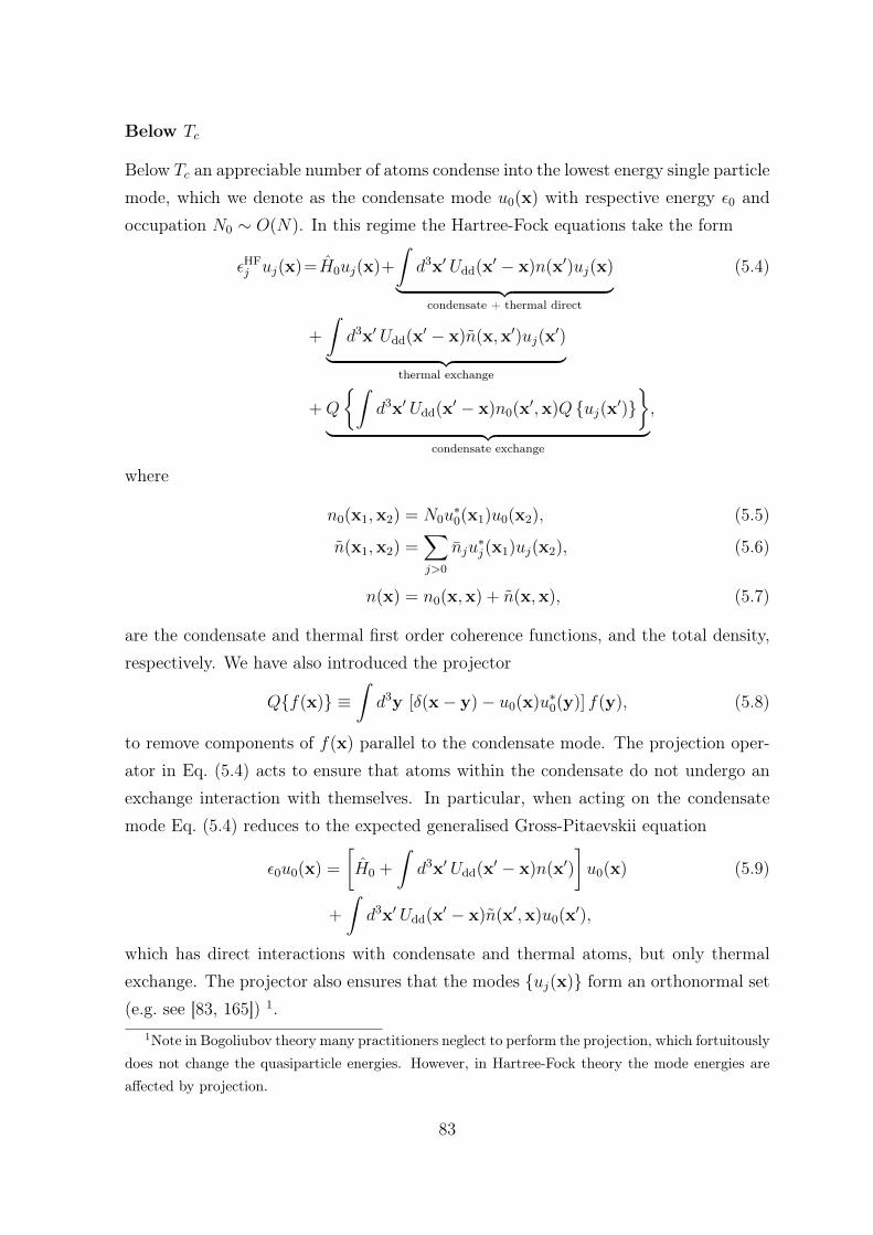
Below Tc
Below Tc an appreciable number of atoms condense into the lowest energy single particlemode, which we denote as the condensate mode u0(x) with respective energy ε0 andoccupation N0 ∼ O(N). In this regime the Hartree-Fock equations take the form
εHFj uj(x)=H0uj(x)+
∫d3x′ Udd(x′ − x)n(x′)uj(x)
︸ ︷︷ ︸condensate + thermal direct
(5.4)
+
∫d3x′ Udd(x′ − x)n(x,x′)uj(x
′)︸ ︷︷ ︸
thermal exchange
+Q
∫d3x′ Udd(x′ − x)n0(x′,x)Q uj(x′)
︸ ︷︷ ︸condensate exchange
,
where
n0(x1,x2) = N0u∗0(x1)u0(x2), (5.5)
n(x1,x2) =∑
j>0
nju∗j(x1)uj(x2), (5.6)
n(x) = n0(x,x) + n(x,x), (5.7)
are the condensate and thermal first order coherence functions, and the total density,respectively. We have also introduced the projector
Qf(x) ≡∫d3y [δ(x− y)− u0(x)u∗0(y)] f(y), (5.8)
to remove components of f(x) parallel to the condensate mode. The projection oper-ator in Eq. (5.4) acts to ensure that atoms within the condensate do not undergo anexchange interaction with themselves. In particular, when acting on the condensatemode Eq. (5.4) reduces to the expected generalised Gross-Pitaevskii equation
ε0u0(x) =
[H0 +
∫d3x′ Udd(x′ − x)n(x′)
]u0(x) (5.9)
+
∫d3x′ Udd(x′ − x)n(x′,x)u0(x′),
which has direct interactions with condensate and thermal atoms, but only thermalexchange. The projector also ensures that the modes uj(x) form an orthonormal set(e.g. see [83, 165]) 1.
1Note in Bogoliubov theory many practitioners neglect to perform the projection, which fortuitouslydoes not change the quasiparticle energies. However, in Hartree-Fock theory the mode energies areaffected by projection.
83

5.2.2 Reduction to Hartree Theory
The full numerical solution of Eq. (5.4) [or even Eq. (5.1)] is extremely challenging,because the thermal exchange requires n(x′,x) to be calculated (or at least applied) foreach self-consistent iteration. This limits the theory to applications involving a smallnumber of modes and away from regimes where mechanical stability can be studied.
The Hartree theory we use is obtained by neglecting both condensate and thermalexchange terms [as labeled in Eqs. (5.4)], yielding
εHFj uj(x) =
[− ~2
2m∇2 + Veff(x)
]uj(x), (5.10)
where the effective potential is
Veff(x) = Vtrap(x) +
∫d3x′ Udd(x− x′)n(x′). (5.11)
The absence of exchange terms means that a projector is no longer needed and noadditional adjustment below Tc (compared to above Tc) is required to account for thecondensate, meaning that the theory smoothly transitions across Tc.
The properties of the Hartree, Hartree-Fock and other theories for the homogeneousBose condensed gas, including conservation laws, are extensively discussed in Sec. VIRef. [166] (also see [167] for a discussion of the HFB and HFBP theories of the inho-mogeneous system). We note that in the uniform purely dipolar gas, the Hartree termis zero and the DDIs affect the system only though the Fock term. However, in thetrapped system the Hartree term is often dominant, particularly when the harmonictrap is appreciably anisotropic (i.e. λ 1 or λ 1).
As discussed in the previous chapter, the neglect of dipole exchange is consis-tent with other work on finite temperature bosons [145] and zero temperature stud-ies of fermion stability [155]. Importantly, Ticknor studied the quasi-two-dimensionalBose gas using the Hartree-Fock-Bogoliubov-Popov (HFBP) meanfield theory [146] andfound that exchange terms were generally less important than direct terms.
We emphasise that our motivation for using this theory is that it includes the dom-inant direct interactions and the full discrete character of the low energy modes, yetis more computationally efficient than Bogoliubov-based approaches. This enables usto study challenging problems that have not been explored, in particular finite tem-perature mechanical stability, in which obtaining convergent self-consistent solutionsis demanding and time consuming.
84

5.2.3 Description of Hartree Algorithm
In this section we discuss our implementation of the Hartree model as a numericalalgorithm.
Semi-Classical Treatment of High Energy Modes
ρ
z
Low E
High E
High E
semiclassical treatment
Low E
discrete modes
Ener
gy
(a) (b)
Figure 5.1: Schematic of our approach to solving dipolar Hartreeequations. (a) The low energy (discrete) modes are explicitly solvedfor by diagonalizing the Hartree equations, whereas higher energymodes are treated using a semiclassical approximation. (b) Schematicof the range of the spatial grids used to solve for the discrete modesand the large grid used to solve for the high energy semiclassicaltheory.
The Hartree equation (5.10) is cylindrically symmetric and can be solved using aset of two-dimensional grids. However, at finite temperature typically & 105 modesare thermally accessible in the regimes we study, and a full self-consistent calculationis not feasible in terms of the discrete (i.e. diagonalised) modes. Instead we employ ahybrid method and diagonalise for the lowest energy modes, up to some energy εcut,and then calculate the remainder within the semiclassical approach [see Fig. 5.1(a)].
The semiclassical approach can be obtained by making the replacement ∇ → ik inEq. (5.10), where k is a wavevector (also see Sec. 4.2). This transforms the Hartree
85

equation to an algebraic equation in which the energy is given in (x,k)-phase-space as
εHF(x,k) =~2k2
2m+ Veff(x). (5.12)
The semiclassical portion of the system is described by a (Wigner) distribution function
W (x,k) =1
eβ[εHF(x,k)−µ] − 1. (5.13)
For consistency the semiclassical description can only be applied to regions of phase-space where ε(x,k) > εcut to avoid double counting of modes. From this we obtain thesemiclassical region density
nsc(x) =
∫
εHF>εcut
d3k
(2π)3W (x,k), (5.14)
=1
λ3dB
ζ3/2
(eβ[µ−Veff(x)], βKmin(x)
), (5.15)
whereζ3/2(z, y) =
2√π
∫ ∞
y
√t
et/z − 1dt (5.16)
is the incomplete Bose function and
Kmin(x) ≡ maxεcut − Veff(x), 0. (5.17)
Summary of Algorithm and Numerical Considerations
All the excitations up to a given energy εcut are solved for using the Arnoldi algorithm.The associated discrete mode density is constructed
nd(x) =∑
εHFj <εcut
nj|uj(x)|2, (5.18)
The semiclassical and the total densities are then evaluated
n(x) = nd(x) + nsc(x). (5.19)
We use fixed point iteration of these steps to ensure self consistency. To avoid oscilla-tions only a small amount of the new prediction for the total density (nnew) is mixedin with the existing prediction (nold), i.e.
n(x)→ λmixnnew(x) + (1− λmix)nold(x), (5.20)
where λmix is the mixing parameter. Upon obtaining a self-consistent solution externalparameters are adjusted to tune the solutions to a desired macrostate (e.g. an outerloop of µ being adjusted to obtain the correct total number N).
We briefly mention a number of aspects of our algorithm:
86

1. We consider gases confined in cylindrically symmetric traps with dipoles alignedalong the z-direction. We thus make use of Fourier-Hankel techniques (seeSec. 3.3) to utilise the cylindrical symmetry and reduce the eigenvalue prob-lem to being two-dimensional. The Fourier-Hankel approach is useful because itallows accurate Fourier transforms to simplify the evaluation of the convolutionrequired to construct the direct dipolar interaction. However, the radial Hankeltransform requires a different radial grid for each angular momentum projectionquantum number m, thus the problem requires a set of two-dimensional grids(we typically diagonalise modes with m up to 10, i.e. requiring 11 grids – gener-ally even more in oblate geometries). This requires extensive transformation ofquantities [e.g. n(x)] between the grids.
2. We use a cutoff dipole interaction potential for improved accuracy and to reducethe size of the numerical grids needed. The cutoff potential minimises interactionbetween aliased copies of the system (problematic with Fourier methods used forsystems with long-range interactions). We make use of both the cylindrical andthe spherical cutoff, see Sec. 3.4.
3. We use two grid extents as schematically shown in Fig. 5.1(b). Since we onlycalculate the discrete modes up to some relatively small energy, εcut, we can usea small and dense set of grids to accurately perform the diagonalizations [andobtain nd(x)]. Then a much larger grid is used for the semiclassical region whichextends out to much higher energy, as needed to accurately capture the thermaltails of the system.
4. In application to mechanical stability, finding self-consistent solutions is chal-lenging and care needs to be taken to ensure that metastable states are not lostprematurely and that a coarse grid does not disguise instability. In using fixedpoint iteration effectively, we employ an algorithm to efficiently increase or de-crease the mixing speed λmix during the self-consistent process. We have observedthat if λmix is too large early on in self-consistency iterations a metastable so-lution may be lost. Normally we start with λmix = 0.3 (∼ 0.01 for biconcavedensity regions) and appropriately increase or decrease this during the search fora self-consistent solutions depending upon conditions. We also note that careneeds to be taken to reliably detect mechanical instability collapse. We performa number of tests to determine instability including detecting the developmentof density spikes and large gaps in the low energy spectrum. We have confirmed
87

that these are good signatures of the grid dependent numerical collapse discussedin Sec. 5.3.2.
5.3 Results
5.3.1 Comparison to Previous Calculations
To benchmark our Hartree calculations we perform a quantitative comparison to theHFBP calculations that Ronen et al. [145] performed for the three-dimensional trappedBose gas at finite temperature. In this subsection we make this comparison for twodifferent sets of results from [145].
We note that those HFBP calculations excluded thermal exchange interactions,although they did include condensate exchange interactions (exchange interaction ofcondensate atoms on the thermal excitations). We extended our Hartree algorithm toinclude condensate exchange but found it made negligible difference to the predictionsand do not include results with this term here.
Condensate Fraction
The results of the first comparison we perform are presented in Fig. 5.2(a). There wecompare the condensate fraction, as a function of temperature, for a system with λ = 7.We observe that the Hartree and HFBP theories predict an appreciably lower conden-sate fraction than the ideal case, and are in very good agreement with each other overthe full temperature range considered. The low energy excitations of a Bose-Einsteincondensate are quasi-particles, which are accurately described by Bogoliubov theory(such as the HFBP theory), however the thermodynamic properties of the system aredominated by the single particle modes (e.g. see [168]). A comparison of the Bogoli-ubov and Hartree-Fock spectra of a T = 0 dipolar Bose-Einstein condensate (BEC) wasmade in [100]. That comparison revealed that the spectra were almost identical, exceptfor low energy modes with low values of angular momentum, where small differencesin the mode frequencies were observed.
Density Oscillating Ground States
An interesting feature of dipolar condensates is the occurrence of ground states withdensity oscillation features, where the condensate density has a local minimum at trapcentre. For a cylindrically symmetric trap these states are biconcave (red blood cell
88

0
0.2
0.4
0.6
0.8
1
N0/N
(a)
0 0.2 0.4 0.6 0.8 10
0.05
0.1
0.15
0.2
0.25
T /T 0c
contr
ast
,c
(b)
Figure 5.2: (a) Condensate fraction and (b) density oscillation con-trast (see text) for a dipolar BEC in a λ = 7 pancake trap. Hartreeresults (pluses), HFBP results (solid lines), ideal gas result (dashedline). HFBP data corresponds to results shown in Figs. 5 and 6of Ref. [145]. Other parameters: ωρ, ωz = 2π × 100, 700 s−1,N = 16.3 × 10³ 52Cr atoms with contact interactions tuned to zero.T 0c = 3
√N/ζ(3)~ω/kB is the ideal condensation temperature, where
ω = 3√ω2ρωz and ζ(α) is the Riemann zeta function with ζ(3) ≈ 1.202.
shaped – surfaces of constant density are shown in Fig. 5.7) first predicted for T = 0
condensates in Ref. [99]. In the purely dipolar case such biconcave states occur undercertain conditions of trap and dipole parameters, but notably only for λ & 6 and fordipole strengths close to instability. In [145] the HFBP technique was used to assessthe effect of temperature on the density oscillating states. This was characterised bythe contrast, a measure of the magnitude of the density oscillation, defined as
c = 1− n(0)
nmax
, (5.21)
where n(0) is the density at trap centre and nmax is the maximum density of the system.
89

In Fig. 5.2(b) we compare our Hartree and HFBP theories for the contrast. Thiscomparison reveals some small residual differences between the theories, however theresults are in reasonable agreement and both predict that the contrast goes to zero(i.e. the condensate returns to having maximum density at trap centre) at T ≈ 0.65T 0
c .
5.3.2 Mechanical Stability
Our first application of the Hartree theory is to study the finite temperature mechanicalstability of a trapped dipolar Bose gas. To do this we construct a phase diagram forthe range of dipole strengths for which the gas is stable for a number of different trapgeometries. Such stability properties, and the dependence on interactions and trapgeometry, have been measured accurately in the dipolar system in the zero temperaturelimit (e.g. see [135]). We note theoretical studies [128, 129, 169] showing the importantrole of temperature on the observed stability of 7Li condensates [3], which have anattractive contact interaction.
Locating the Stability Boundary
We consider a trapped sample of fixed mean number N and wish to determine thevalues of the dipole interaction parameter for which the system is mechanically stableas a function of temperature. In doing so we construct a phase diagram in Cdd, T-space that indicates the stable region. In practice we locate the stability boundary(i.e. a curve) that separates the stable and unstable regions. Our procedure to obtainthis boundary involves a computationally intensive search through parameter space tofind the self-consistent solutions on the verge of instability. Determining the stabilityboundary for fixed mean number N complicates this process: since we work in thegrand-canonical ensemble where the proper variables are µ,Cdd, T, an additionaliterative search over the parameter µ is required to fix N to the desired target number.
In Fig. 5.3 we provide some examples to illustrate how we identify the value of theDDI at the stability boundary for a gas with (target number) N = 2× 10⁵ atoms at aparticular temperature. To do this we show the dependence of total atom number onµ for two different values of the DDI [Fig. 5.3(a)]. For both curves the total numberincreases as we move along these curves until some maximum value Ncrit is reachedat which the system becomes unstable. The non-monotonic behavior of these curvesarises because the ground state energy ε0 changes as the number of atoms increases,and hence the role of DDIs increases. For this reason we also show the same two cases,
90

-1 0 1 20
1
2
3
4x 10
5
µ/ hω
Ato
m N
um
be
r
(a)case B
case A
0 1 2 30
1
2
3
4x 10
5
( 0 − µ)/ hω
(b)
0 0.5 1 1.5 20
1
2
3
4
5x 10
4
ρ, z /a ho
na
3 ho
(c)
0 5 10 15 20 250
10
20
30
40
ρ, z /a ho
(d)
target N
Ncrit
Ncrit
condensation
uncondensed
Figure 5.3: Locating instability (upper subplots): (a) The to-tal number of atoms of the self-consistent Hartree solution ver-sus chemical potential for λ = 1/8, kBT = 40~ω and Cdd =
7× 10⁻⁴~ωa3ho (dashed, case A), 1.5× 10⁻⁴~ωa3
ho (solid, case B), withaho =
√~/mω. Each line terminates at the point of instability and
occurs at the respective critical number Ncrit. (b) Same results asin (a) but plotted against ε0 − µ. The dotted line represents thetarget number, in this case N = 2 × 10⁵. Density Profiles (lowersubplots): Solid (dashed) line represents the radial (axial) density n,higher curves are near the stability boundary. λ = 1, N = 2 × 10⁵.(c) T/T 0
c = 0.82 (N0/N ≈ 0.43) and Cdd/4πC0 = 3.65 × 10⁻⁴
(gray), 1.83× 10⁻⁴ (black). (d) T/T 0c = 1.27 and Cdd/4πC0 = 2.91
(gray), 1.22 (black). We have used the interaction strength unitC0 = ~ωa3
ho/6√N which is convenient for cases where N is fixed. Note
that in this figure ε0 ≡ εHF0 .
91

but as a function of εHF0 − µ, in Fig. 5.3(b).
The sharp cusps in Figs. 5.3(a) and (b) correspond to the point where the systemcondenses [i.e. where εHF
0 −µ ≈ 0]. The dependence of εHF0 on N0 is strongly dependent
on the trap geometry, and for the cases we consider here with λ = 1/8, εHF0 decreases
with increasing N0. This is because the head-to-tail character, in the cigar geometry,emphasises the attractive part of the DDI so that as the condensate number increases,εHF
0 (≈ µ) decreases.
For case A in Fig. 5.3(a) the number at which collapse occurs is less than the targetnumber, thus we conclude that the DDI used in this calculation lies within the unstableregion for the system (i.e. no stable solution can be found for N atoms with this valueof DDI). In contrast, for case B in Fig. 5.3(a) Ncrit > N and thus the value of DDI isin the stable region. To locate the stability boundary points we need to trace out thesecurves for various Cdd values until we find Ncrit = N to within our numerical tolerance(this has to be done for each value of T ). This process is painstaking and can takeseveral days to find a single point on the stability boundary.
We identify the self-consistent Hartree solutions as being unstable when they be-come grid-dependent. This means that as the distance between grid points tends tozero, the radial width of the cloud contracts and the chemical potential tends to neg-ative infinity. Precisely locating the instability point is a stringent numerical task andrequires careful convergence tests. For condensates with contact interactions this typeof numerical instability analysis was applied in Refs. [128, 129, 169] (also see Ref. [72]).In Fig. 5.3(a) the instability point occurs at the end of the upper horizontal plateau inthe N versus µ curves (compare to Fig. 1 of [128]). We show examples of the spatialdensity profiles for a spherical trap in Figs. 5.3(c) and (d). The system considered inFig. 5.3(c) is condensed, while that considered in Fig. 5.3(d) is above the critical tem-perature. For both cases a result is shown that is well inside the stable region (blackcurves) and near the stability boundary (gray curves). Despite a large difference in thedensity scales of the two regimes they both exhibit a similar sharpening of the densityprofile near instability.
An additional consideration emerges for stability calculations below Tc in regimeswhere the condensate is in a density oscillating state. Here the first mode to go soft (andthen develop imaginary parts) as the stability boundary is reached is a m 6= 0 quasi-particle mode [121], where m is the angular momentum projection quantum number(so called angular roton mode [99]). This instability is not revealed in the Hartreeexcitations, and as we solve for the condensate in the m = 0 space (see Sec. 5.2.3), the
92

condensate does not exhibit numerical instability. Thus in cases where the condensateexhibits a density oscillating state we perform a Bogoliubov analysis of the condensatemode (within the effective potential of the self-consistent Hartree solution) to determineif any m 6= 0 modes have become unstable 2.
Stability Above Tc
0.9 1 1.1 1.2 1.3
0
1
2
3
4
5
6
7
8
T / T 0c
Cdd/4πC
0
unstableλ = 8
λ = 4
λ = 2
λ = 1
λ = 1 / 2
λ = 1 / 8
Hartreesemiclassical
Figure 5.4: Stability regions in DDI-temperature space. Shaded re-gions indicate stability for each geometry, from top to bottom λ =
8, 4, 2, 1, 1/2, 1/8, the geometric mean trap frequency is fixed andN = 2 × 10⁵. Actual data points represented by symbols while theshading of the stable regions interpolates to guide the eye, the semi-classical model is given by the solid curves. Error bars represent the1 σ spread in the convergence test (see Sec. 5.3.3 for more details).
In Fig. 5.4 we show our results for the stability of the normal phase. In chapter4 we examined this regime using a semiclassical Hartree approach which are shown
2For an analogous calculation, but at T = 0, see [100]
93

here as solid lines in Fig. 5.4. We observe that as a general trend the stability regiongrows with increasing λ. The strong geometry dependence of these results arises fromthe anisotropy of the dipole interaction: In oblate geometries (λ > 1) the dipoles arepredominantly side-by-side and interact repulsively (stabilizing), whereas in prolategeometries (λ < 1) the attractive (destabilizing) head-to-tail interaction of the dipolesdominates (a similar geometry dependence is observed for the stability of T = 0 dipolarcondensates [99, 109]).
A primary concern is the nature of beyond semiclassical effects, i.e. what differencesemerge from our diagonalised Hartree theory over the semiclassical formulation. Mostprominently in the results of Fig. 5.4 we observe that while the Hartree and semiclassicalstability boundaries are in good agreement for prolate geometries, in oblate traps theHartree results are significantly more stable. This difference between the boundariespredicted by the two theories increases with increasing λ. This observation is surprisingbecause our calculation is for a rather large number of atoms (N = 2 × 10⁵), wherethe semiclassical approximation would normally be expected to furnish an accuratedescription of the above Tc behavior.
We attribute this failure of the semiclassical theory to its inappropriate treatment ofthe interactions between the low energy modes 3. The nature of the DDI, when tightlyconfined along the polarization direction, has been extensively studied in application topure BECs [110, 113], where it has been shown that it confers additional stability on thesystem, as verified in recent experiments [138]. This arises from a confinement inducedmomentum dependence of the interaction: the interaction is repulsive (stabilizing)for low momentum interactions, but decays to being attractive with a characteristicwavevector k ∼ 1/az set by the z confinement length az =
√~/mωz. Notably these
features of the confined interaction mediate BEC instability through the softening ofradially excited modes with a wavelength ∼ az [75, 110–112, 118].
It is not clear that these confinement effects will be applicable at a modestly oblatetrap with λ = 8, however numerical studies have revealed that quasi-particle modeswith a wavelength ∼ az soften in a BEC with λ = 7 [99]. Within the limited rangeof results we have for λ > 1 we see evidence consistent with confinement induced ef-fects playing an important role in the above Tc Hartree calculations. Notably, that therelative difference between the stability boundaries of the Hartree and semiclassical cal-culations scale with 1/a2
z. Also, when the system is unstable, during the self-consistency
3For definiteness, this discussion relates to the in-plane interaction between atoms in the lowest zvibrational mode.
94

iterations (prior to collapse) strong radial density fluctuations develop in the system
A key prediction from our semiclassical study [72] is a double instability feature inoblate trapping geometries arising from the interplay of thermal gas saturation and theanisotropy of the DDI. Our Hartree calculations in this oblate regime, despite shiftingthe stability boundary from the semiclassical prediction by a considerable amount,reveal that the double instability feature is robust to beyond-semiclassical effects.
A prominent feature of the semiclassical calculation is that the stability curves forthe purely dipolar gas terminate at the critical point with Cdd = 0 (i.e. predictingthat without contact interactions only an ideal gas is stable below Tc). This occursbecause the local compressibility at trap centre diverges at the critical point and thegas is unstable to any attractive interaction (see [72]). In the beyond-semiclassicalcalculations the trap provides a finite momentum cutoff that prevents the divergenceof compressibility, and thus the system has a finite residual stability at and below Tc,which we consider next.
Stability Below Tc
In Fig. 5.5 we consider the stability below Tc where the semiclassical model does notapply. These results are identical to those shown in Fig. 5.4, but the below Tc detailsare revealed using a logarithmic vertical axis. Compared to the above Tc gas the con-densate is rather fragile, with the critical DDI strength defining the stability boundarydecreasing by ∼3 to 4 orders of magnitude.
In the zero temperature limit our results agree with previous calculations basedon solving the Gross-Pitaevskii equation [99]. This agreement is expected as the twotheories are identical when the excited modes have vanishing population. For a purecondensate, the critical DDI strength depends on the condensate number and trapgeometry according to [99]
C?dd =
F (λ)
N0
, (T = 0) (5.22)
with F (λ) a rather interesting function of trap geometry alone, as characterised inFig. 1 of [99] 4. More generally, beyond the case of pure DDIs, F also depends on thecontact interaction strength, e.g. see [75, 109].
4Note we use fixed geometric mean trap frequency, whereas [99] fixes ωρ. The interaction parameterused in [99] (N 1 limit) isD = NCdd/4π~ωρa3ρ) with aρ =
√~/mωρ, which relates to our parameter
as D = N5/6λ−1/6Cdd/4πC0.
95

0 0.2 0.4 0.6 0.8 1 1.2
10-4
10-3
10-2
10-1
100
T λ=1c,FST λ=8
c,FS
T /T 0c
Cdd/4π
C0 unstable
λ = 8
λ = 1/8Hartre e
Semic l assi cal
Figure 5.5: Stability boundary focusing on the below Tc behavior(line styles as in Fig. 5.4). For reference the ideal finite size adjustedcritical temperature Tc,FS [104] for two geometries (T λ=1
c,FS and T λ=8c,FS)
are indicated by short vertical lines. The effect of DDIs on Tc wascalculated perturbatively in [170, 171], however our results are faroutside the perturbative regime.
As temperature increases, but focusing on T < T 0c , we observe in Fig. 5.5 that
the stability boundary increases significantly. This occurs because as the temperatureincreases the condensate is thermally depleted. Indeed, by simply accounting for thethermal depletion we can immediately extend result (5.22) to predict the critical valueof the DDI at finite temperature C?
dd(T ):
C?dd(T ) =
F (λ)
N0(T )= C?
dd(0)N
N0(T ), (5.23)
where the last expression is obtained using N0(T = 0) = N . Equation (5.23) predictsthat the stability at finite temperature increases inversely proportional to the conden-sate occupation and, as shown in Fig. 5.6, provides a good description of the stabilitypredictions from the full Hartree calculations. In these comparisons we have used two
96

0 0.2 0.4 0.6 0.8 1
10-4
10-3
10-2
T /T 0c
Cdd/4π
C0
λ = 8
λ = 1/8
λ = 1
unstable
Figure 5.6: Stability boundary scaling. The stability boundary results(symbols) have been taken from Fig. 5.5 for λ = 8,1,1/8 (top tobottom). Dashed line prediction is based on a non-interacting N0
scaling (see text) and the solid line uses the N0 calculated from theHartree solutions.
models for the condensate occupation: (i) the non-interacting prediction
NNI0 (T ) = N [1− (T/T 0
c )3], (5.24)
and (ii) the value of N0(T ) obtained from the Hartree calculations. Equation (5.23)using NNI
0 (T ) provides a good prediction for Hartree stability curves with λ = 1/8 and1. For the oblate system (λ = 8) agreement is not as good as is apparent in Fig. 5.5for T & 0.5T 0
c . In this case the values of Cdd at the stability boundary are much higherthan for the other values of λ, and thus interaction effects more significantly affect thecondensate. However, much better agreement is obtained if we take N0(T ) from theHartree solution.
We note that the simple model (5.23) does not account for any other effects of thethermal cloud on the condensate [e.g. thermal back action through modifications of
97

Veff(x)]. Thus, the level agreement of this simple model with the full Hartree resultssuggest that these additional effects are not significant in the regimes we have studied.
5.3.3 Convergence Tests of Stability Boundary
In oblate geometries the self consistent calculations above Tc become increasingly dif-ficult to perform as λ increases. For this reason we have not extended our calculationsbeyond λ = 8. The origin of the difficulty is two fold: (i) the effective potential flattensconsiderably which increases the low energy density of states, meaning that a largenumber of modes exist below εcut. (ii) In oblate geometries the interaction strengthsat instability are much larger, and these numerous low energy modes interact stronglywith each other.
The important convergence test is that our results are independent of the bound-ary (εcut) separating the discrete low energy modes from the continuous semiclassicalspectrum. The typical error bars shown in Figs. 5.4 and 5.5 represent the variationin the stability boundary as εcut was varied (1 σ spread obtained from tests where thenumber of discrete modes ranged over ∼ 10 to 1000). It is not computationally feasiblefor us to take εcut high enough for λ ≥ 4 (above Tc) to get a self-consistent result fullyindependent of εcut. However, note we do not observe a systematic drift nor monotonicrelationship between εcut and the stability boundary.
Below Tc the error bars are instead determined arbitrarily by the bisection toleranceof parameters µ and Cdd.
5.3.4 Thermal Effects on Biconcavity
As our final application we consider thermal effects on the biconcave density profileswhich occur in oblate geometries. To date, the only study of temperature effects of thesestates was in Ref. [145] [which we reproduce in Fig. 5.2(b)]. That study considered asingle line (at fixed Cdd and N and varying T ) through the phase diagram, and showedthat biconcavity persisted at small finite temperatures (T . 0.25T 0
c ), but then wasrapidly washed out as temperature increased further.
Using our Hartree theory we provide a broad characterization of the thermal effectson biconcavity. We focus on the case λ = 8, which supports a biconcave condensateat T = 0. In Fig. 5.7(a) we present contours of biconcave contrast [as defined inEq. (5.21)] over the entire range of parameters where this state is stable. These resultsshow that biconcavity is not destroyed as temperature increases. Instead the parameter
98

6
of λ, and thus interaction effects more significantly effect thecondensate. However, much better agreement is obtained inwe take N0(T ) from the Hartree solution.
We note that the simple model (9) does not account for anyother effects of the thermal cloud on the condensate [e.g. ther-mal back action through modifications of Veff(x)]. Thus, thelevel agreement of this simple model with the full Hartree re-sults suggest these additional effects are not significant in theregimes we have studied.
C. Thermal effects on biconcavity
As our final application we consider thermal effects on thebiconcave density profiles which occur in oblate geometries.To date, the only study of temperature effects of these stateswas in Ref. [18] [which we reproduced in Fig. 1(b)]. Thisstudy, considered a single line (at fixed Cdd and N , and vary-ing T ) through the phase diagram, and showed that biconcav-ity persisted at small finite temperatures (T 0.25T 0
c ), butthen was rapidly washed out as temperature increased further.
Using our Hartree theory we provide a more broad char-acterization of the thermal effects on biconcavity. We focuson the case λ = 8, which supports a biconcave condensateat T = 0. In Fig. 6 we present contours of biconcave con-trast [as defined in Eq. (6)] over the entire range of parameterswhere this state is stable. These results show that biconcavityis not destroyed as temperature increases. Instead the param-eter region over which biconcavity occurs grows, with largebiconcave contrasts emerging at higher temperature. The gen-eral trends seen can be understood by considering the ther-mal depletion of the condensate, using similar arguments tothose made to obtain Eq. (9): as the temperature increases athe value of Cdd required for the condensate to exhibit a bi-concave density profile should increase in a manner that isapproximately inversely proportional to the condensate occu-pation. Thus, the washing out observed in [18] [our Fig. 1(b)]arises because they considered Cdd fixed. Thermal depletionof the condensate is not sufficient to explain all aspects ob-served, e.g. the deepening of the biconcave contrast. Thisarises from additional effects of the thermal interaction withthe condensate, e.g. small changes in the aspect ratio of the ef-fective potential from the condensate can significantly changethe contrast (c.f. Fig. 1 of Ref. [11]).
In Fig. 6 (lower) we show two examples of the biconcavedensity profiles at different temperatures. Case B displaysthe very pronounced biconcavity for a system at T ≈ 0.9T 0
c ,where the condensate fraction is N0/N ≈ 0.07.
IV. CONCLUSIONS
In this paper we have developed a Hartree theory for atrapped dipolar Bose gas that can be applied to make predic-tions above and below the critical temperature Tc for conden-sation. We have used this theory to quantify the role of ther-mal fluctuations on the mechanical stability of the cloud, andpresent results for the stability phase diagram as a function of
0 0.2 0.4 0.6 0.8 1
0
0.01
0.02
0.03
0.04
0.05
0.06
T /T 0c
Cdd/4πC
0
A
B
(a)
0 2 4 6 8 10 120
500
1000
1500
2000
2500
3000
ρ/aho
density
×a3 ho
A
B
(b)
0.86 0.88 0.9 0.920
0.01
0.02
0.03
0.04
0.05
0.06
unstable
B
FIG. 6. (Color online) Biconcave characteristics for λ = 8 andN = 2 × 10⁵ at finite temperature. (a) Stability diagram for λ = 8from Fig. 3 with biconcave contrast contours 0, 0.05, 0.1, 0.15, 0.2,0.25 (bottom to top) added. The solid curves are interpolations be-tween the calculated contours points. The white dotted line markswhere we terminate the contours due to the condensate fraction be-coming negligibly small. Triangles indicate the stability boundaryfrom Fig. 5. Inset: Magnification of the high temperature region.(b) Radial densities for phase space points marked by A and B ofthe upper figure. A: T/T 0
c = 0.0910, Cdd/4πC0 = 0.00268 andN0/N = 1.00 (thermal depletion < 1%). B: T/T 0
c = 0.910,Cdd/4πC0 = 0.0291 and N0/N = 0.0716. Solid (dashed) linesrepresent the total (condensate) density. Insets: corresponding sur-face contour at 67% of the peak density.
temperature and aspect ratio. Our results show that the ther-mal depletion of the condensate can lead to an enhancementof the parameter regime over which biconcave density oscil-lations are found. Furthermore, a large thermal cloud mayactually enhance the biconcave contrast making direct imag-ing of an in situ blood cell more feasible, see Fig. 6 (lower).Above Tc we find that the results of our theory predict signif-icant corrections to the stability boundary over the equivalentHartree semiclassical theory. Most notably, the semiclassicaltheory underestimates the size of the stability region for oblate
Figure 5.7: Biconcave characteristics for λ = 8 and N = 2 × 10⁵
at finite temperature. (a) Stability diagram with biconcave contrastcontours 0, 0.05, 0.1, 0.15, 0.2, 0.25 (bottom to top) added. Thesolid curves are interpolations between the calculated contour points.The white dotted line marks where we terminate the contours dueto the condensate fraction becoming negligibly small. Triangles indi-cate the stability boundary from Fig. 5.5. Inset: Magnification of thehigh temperature region. (b) Radial densities for phase space pointsmarked by A and B in (a). A: T/T 0
c = 0.0910, Cdd/4πC0 = 0.00268
and N0/N = 1.00 (thermal depletion < 1%). B: T/T 0c = 0.910,
Cdd/4πC0 = 0.0291 and N0/N = 0.0716. Solid (dashed) lines rep-resent the total (condensate) density. Insets: corresponding surfacecontours at 67% of the peak density.
99

region over which biconcavity occurs grows, with large biconcave contrasts emergingat higher temperature. The general trends seen can be understood by consideringthe thermal depletion of the condensate, using similar arguments to those made toobtain Eq. (5.23): as the temperature increases the value of Cdd required for thecondensate to exhibit a biconcave density profile should increase in a manner that isapproximately inversely proportional to the condensate occupation. Thus, the washingout observed in [145] [our Fig. 5.2(b)] arises because they considered Cdd fixed. Thermaldepletion of the condensate is not sufficient to explain all aspects observed in our results,e.g. the deepening of the biconcave contrast that develops at higher temperatures inFig. 5.7(a). This arises from additional effects of the thermal interaction with thecondensate, e.g. small changes in the aspect ratio of the effective potential that thecondensate experiences can significantly change the contrast (c.f. the strong dependenceof biconcavity on trap aspect ratio near λ = 8 in Fig. 1 of Ref. [99]).
In Fig. 5.7(b) we show two examples of the biconcave density profiles at differenttemperatures. Case B displays the very pronounced biconcavity for a system at T ≈0.9T 0
c , where the condensate fraction is N0/N ≈ 0.07.
5.4 Conclusions
In this chapter we have developed a Hartree theory for a trapped dipolar Bose gasthat can be applied to make predictions above and below the condensation temper-ature. We have used this theory to quantify the role of thermal fluctuations on themechanical stability of the cloud, and present results for the stability phase diagramas a function of temperature and aspect ratio. Above Tc our theory predicts significantcorrections to the stability boundary over the equivalent semiclassical theory. Most no-tably, the semiclassical theory underestimates the size of the stability region for oblategeometries. Below Tc (but at finite temperature) we find that the stability boundary iswell described by the zero temperature result after scaling for the thermally depletedcondensate.
We have also studied the role of thermal fluctuations on biconcave condensatestates. Our results show that as temperature increases, and the condensate thermallydepletes, the range of interaction parameters in which these kinds of states can be foundincreases. Furthermore, a large thermal cloud may actually enhance the biconcavecontrast making direct imaging of an in situ density oscillating state more feasible, seeFig. 5.7(b).
100

An important step for future theoretical studies in the finite temperature regime isto fully include thermal exchange effects. Because a large number of modes are impor-tant for temperatures of the order of Tc, full Hartree-Fock calculations will probablynot be feasible. It is possible to include exchange interactions semiclassically (c.f. Fermistudies [98, 151]), although our work here has shown beyond semiclassical effects areimportant even above Tc. An interesting possibility is the extension of classical fieldmethods to thermal dipolar gases (e.g. [172–175]) which may provide a comprehensivedescription for temperatures around the condensation transition.
101

102

Part II
Rotons and Fluctuations in a Trapped
Dipolar Condensate
103


Chapter 6
Fluctuations of a Roton Gas
6.1 Introduction
To date there has been no experimental evidence for the existence of rotons in dipolarcondensates, and increasing attention is turning to developing signatures for detect-ing their presence, such as structure formation in the ground state density profiles[99, 107, 109, 176], anisotropic superfluidity [111, 118] and sensitivity to perturbations[75, 177, 178]. Experimentally, rotons will likely be realised in pancake shaped traps(or an array of pancake traps, e.g. see [138]), and the trap itself plays a very fun-damental role in the nature of the rotons that emerge [99]. In particular the rotonsare sensitive to the condensate density, which decreases away from trap centre due tothe weak radial trapping. As a result the rotons are effectively confined to the cen-tral region of the condensate realising what has been termed a confined roton gas [122].
In this chapter we consider a radially symmetric pancake trapping potential withλ = 20. Our fully 3D calculations find the condensate by solving the GP equations (seeSec. 3.5) while excitations are treated within a Bogoliubov framework (see Sec. 3.6),our results show that the rotons have an essential 3D character. We note that otherwork in this area has focused on close-to-spherical traps [99, 179, 180] or has been inthe quasi-2D regime [146, 181, 182].
We demonstrate that measurements of atom number fluctuations in a trapped dipo-lar condensate is a sensitive probe to reveal the presence of the elusive roton excitation.The key signature is a super-Poissonian peak in the fluctuations as the size of the mea-surement cell is varied, with the maximum occurring when the size is comparable tothe roton wavelength. The magnitude of this roton feature is enhanced significantly
105

for relatively low temperatures (well below Tc). While our main results are based onfull numerical solutions of the meanfield equations, we also develop and validate asimple local density theory. We find that fluctuations reveal rotonic behaviour that isqualitatively different in the trapped gas as compared to the quasi-2D uniform case.
This chapter covers our works accepted to Phys. Rev. Lett. [76] and currently underreview by Phys. Rev. A [74]. An additional paper for detailing the numerical techniquesfor calculating fluctuations within cells is currently in preparation.
6.1.1 Number Fluctuations Within Cells
In this chapter we investigate how rotons manifest themselves in the fluctuations ofa dipolar BEC. This is motivated by significant developments made in BEC imagingsystems to allow precise in situ measurements of density (e.g. see [163]). Such mea-surements actually determine the atom number Nσ within a finite sized cell σ, withthe cell parameters determined by the imaging system [183].
In equilibrium the number fluctuations
δN2σ ≡ 〈N2
σ〉 −N2σ , (6.1)
about the mean number Nσ ≡ 〈Nσ〉 are crucially dependent on the cell size [184]: forcells smaller than all relevant length scales (i.e. healing length and thermal de Brogliewavelength) the fluctuations are Poissonian δN2
σ = Nσ (known as the shot-noise limit),whereas for large cells the thermodynamic result holds
δN2σ = NσkBTnκT , (6.2)
with n the density and κT the isothermal compressibility. In the high temperaturelimit the compressibility becomes classical,
κT =1
nkBT, (6.3)
and again [inserting Eq. (6.3) into Eq. (6.2)] the shot-noise limit is reached.DDIs introduce two important features for fluctuations: (1) the roton wavelength
introduces a new length scale which is revealed as the cell size changes; (2) the attractivenature of the interaction for short wavelengths induces enhanced fluctuations, this is incontrast to the suppression of fluctuations expected in a condensate with short rangeds-wave interactions 1.
1Large BECs with purely contact interactions are only stable when as > 0, which suppresses longwavelength fluctuations.
106

Figure 6.1: Schematic geometry of the system we consider: a radiallysymmetric pancake condensate realised by tight confinement along z;cylinder and washer-shaped cells in which number fluctuations aremeasured. The cylindrical cell is parameterised by the radius R fromtrap centre to the cylinder axis, and its diameter D. The washer-shaped cell is centred on the trap centre, and is parameterised by themid-radius R and width W . For both cells the z extent is taken tobe larger than the condensate thickness.
The geometry of the tightly confined (pancake) dipolar condensate and the typesof cells in which we measure number fluctuations are shown in Fig. 6.1. The twocell shapes we consider are cylindrical and washer-shaped cells with the z extent ofthese cells being larger than the condensate thickness in this direction. The cylindricalcell can be realised experimentally using absorption imaging (column density along z)with the minimum diameter (D) being set by the spot size 2 of the imaging system(e.g. see [183, 185, 186]). These measurements are made using a charged coupled device(CCD) in which the pixel size is typically much smaller than the spot size. Cells withmore general shapes in the xy-plane can be realised by collecting signal from a set ofpixels, e.g. larger diameter cylinders and the washer-shaped case that we consider later.
2The spot size is representative of the diffraction and aberration limited image size of a point-likesample [183]
107

6.2 Local Density Fluctuations
Before considering number fluctuations within cells we take a detour and in this sectionwe consider local density fluctuations, focusing on the regime where a roton-like exci-tation spectrum develops. As is the case for the majority of this chapter our results areobtained by solving the GPE and BdG equations (see Secs. 3.5 and 3.6, respectively)for a dipolar BEC in a pancake trap (λ = 20). We report on the behavior of a numberof key quantities that characterise the system, including the non-condensate densityand density fluctuations; elucidating remarkable properties of the roton gas.
6.2.1 Density of a Confined Roton Gas
We follow Ref. [100] and introduce C = Nas/aρ andD = 3Ngddm/4π~2aρ as the dimen-sionless contact interaction and DDI parameters, respectively 3. The non-condensatedensity, given by [see Eq. (3.36)]
n(x) ≡ 〈δ†δ〉 =∑
j
[nj|uj(x)|2 + (nj+1)|vj(x)|2
], (6.4)
characterises the atoms excited out of the condensate due to interactions and thermaleffects, where nj is the Bose-Einstein distribution,
nj = 〈α†jαj〉 =1
exp(εj/kBT )− 1. (6.5)
In Figs. 6.2(a1) and (b1) we show the non-condensate density for systems in apancake shaped trap at a small, but non-zero temperature. The result in Fig. 6.2(a1) isfor a condensate with only dipole interactions (i.e. D = 220, C = 0), while Fig. 6.2(b1)is for a contact interaction only case (i.e. D = 0, C = 127). The values of theinteraction parameters were chosen to ensure than both cases had approximately thesame chemical potential (µ ≈ 37.5~ωρ), which leads to the condensate modes beingquite similar [e.g. see condensate density contours shown in the insets to Figs. 6.2(a1)and (b1)]. The value D = 220 is sufficiently large to reveal the effects of DDIs onthe system, yet is still well in the stable region (about 10% below the critical valueat which the system becomes dynamically unstable). Indeed, for these parameters thesystem exhibits a roton-like feature in its excitation spectrum [see Fig. 6.2(a2), anddescription below], and associated with this is a prominent peak in the non-condensate
3Note that D also represents the diameter of cylindrical cells. However, throughout section 6.2 wedo not consider cells at all and D will always represent the dimensionless DDI parameter.
108
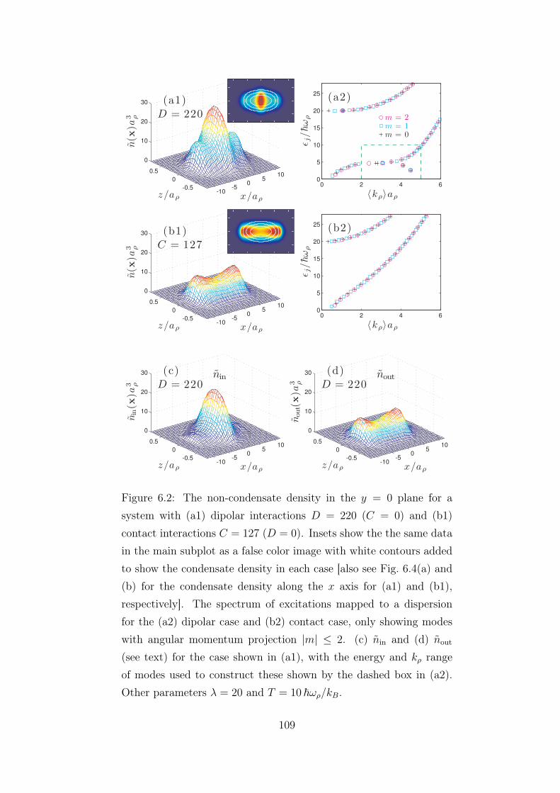
-10-5
05
10
-0.5
0
0.5
0
10
20
30
x/aρz/aρ
(a1)D = 220
n(x
)a3 ρ
0 2 4 60
5
10
15
20
25
m = 0m = 1m = 2
〈kρ〉aρ
ǫ j/hω
ρ
(a2)
-10-5
05
10
-0.5
0
0.5
0
10
20
30
x/aρz/aρ
(b1)C = 127
n(x
)a3 ρ
0 2 4 60
5
10
15
20
25
〈kρ〉aρ
ǫ j/hω
ρ
(b2)
-10-5
05
10
-0.5
0
0.5
0
10
20
30
x/aρ
nin
z/aρ
(c)D = 220
nin(x
)a3 ρ
-10-5
05
10
-0.5
0
0.5
0
10
20
30
x/aρ
nout
z/aρ
(d)D = 220
nou
t(x)a
3 ρ
Figure 6.2: The non-condensate density in the y = 0 plane for asystem with (a1) dipolar interactions D = 220 (C = 0) and (b1)contact interactions C = 127 (D = 0). Insets show the the same datain the main subplot as a false color image with white contours addedto show the condensate density in each case [also see Fig. 6.4(a) and(b) for the condensate density along the x axis for (a1) and (b1),respectively]. The spectrum of excitations mapped to a dispersionfor the (a2) dipolar case and (b2) contact case, only showing modeswith angular momentum projection |m| ≤ 2. (c) nin and (d) nout
(see text) for the case shown in (a1), with the energy and kρ rangeof modes used to construct these shown by the dashed box in (a2).Other parameters λ = 20 and T = 10 ~ωρ/kB.
109

density near trap centre [see Fig. 6.2(a1)], which we refer to as the roton peak. Thisroton peak in n is absent in the contact only case, which instead has a local minimum(along the x-axis) at trap centre [see Fig. 6.2(b1)]. It is also important to take note thatthe roton peak exhibits a greater z-extent than the parts of n away from trap centre.This indicates that the excitations responsible for the roton peak have some important3D character and would not be accurately captured in the quasi-2D treatment in whichthe z-motion is essentially frozen out (also see [113]). This reaffirms the necessity ofthe full 3D numerical solution we provide here.
To quantify the nature of excitations in the trapped system we follow the procedureintroduced in [118] to approximately map the excitations to a dispersion relation. Inthis procedure each quasiparticle is assigned a momentum according to
〈kρ〉j ≡√∫
d3k k2ρ [|uj(k)|2 + |vj(k)|2]∫
d3k [|uj(k)|2 + |vj(k)|2], (6.6)
whereuj(k) =
∫d3xe−ik·xuj(x), vj(k) =
∫d3xe−ik·xvj(x), (6.7)
are the quasiparticle amplitudes in momentum space. The result of this analysis for thepurely dipolar case [see Fig. 6.2(a2)] reveals a clear flattening in the dispersion relationfor 2/aρ . 〈kρ〉j . 5/aρ, as well as some particular modes dropping down. The upperbranch of excitations (εj ≥ 20~ωρ) in this figure corresponds to modes that are excitedin the tightly confined z-direction. For the contact interaction case [see Fig. 6.2(b2)] astrong phonon-like (linear) dispersion is apparent, with no roton-like softening in the〈kρ〉j range where it occurs for the dipolar case.
To verify the relationship between the roton-like part of the spectrum and theroton peak in the non-condensate density we define nin as the non-condensate densitycalculated according to Eq. (6.4) but with the summation over modes restricted tothose satisfying 〈kρ〉j ∈ [2/aρ, 5/aρ] and εj < 10~ωρ. The boundaries of this region areindicated by the dashed box in Fig. 6.2(a2), and were selected to include the modeswhere the roton-like softening is observed. We define nout to be the non-condensatedensity arising from all other modes, such that n = nin + nout. In Fig. 6.2(c) we shownin for the dipolar case, verifying that the roton peak arises from modes in the rotonregion. Furthermore, nout, shown in Fig. 6.2(d), is very similar to the contact case[c.f. Fig. 6.2(b1)], since the character of long wavelength excitations (i.e. those with〈kρ〉j < 2/aρ) for the two cases [compare Figs. 6.2(a2) and (b2)] are similar.
The localised nature of the roton-like excitations for a pancake shaped dipolarBEC was revealed in previous numerical studies that examined individual excitations
110

-10-5
05
10
-0.50
0.5
0
10
20
30
x/aρz/aρ
D = 80
(a1)
n(x
)a3 ρ
0 2 4 60
2
4
6
8
10
m = 0
m = 1
m = 2
〈kρ〉aρ
ǫ j/hω
ρ
(a2)
-10-5
05
10
-0.50
0.5
0
10
20
30
x/aρz/aρ
D = 140
(b1)
n(x
)a3 ρ
0 2 4 60
2
4
6
8
10
〈kρ〉aρ
ǫ j/hω
ρ
(b2)
-10-5
05
10
-0.50
0.5
0
10
20
30
x/aρz/aρ
D = 200
(c1)
n(x
)a3 ρ
0 2 4 60
2
4
6
8
10
〈kρ〉aρ
ǫ j/hω
ρ
(c2)
Figure 6.3: Development of a roton peak in the non-condensate asthe dipole interaction increases. Non-condensate density in the y = 0
plane for (a1) D = 80, (b1) D = 140, (c1) D = 200, with respec-tive mapped dispersions in (a2)-(c2). Insets show the non-condensatedensity with white lines indicating contours of the condensate density.Note: C = 0 in all these results.
[75, 99]. More recently, Jona-Lasinio et al. [122] have proposed the idea of a confinedroton gas based on a local density analysis of a trapped dipolar condensate. Theiranalysis shows that the sensitivity of the roton excitations to the condensate density
111

effectively confines these excitations to a small region near the trap centre, and explainsthe roton peak in n we observe.
In Fig. 6.3 we show how the density peak in n develops for several values of thedipolar interaction strength. The peak is absent for low interaction strengths, wherethe excitation spectrum is monotonically increasing with 〈kρ〉 [Fig. 6.3(a1), (a2)]. Thepeak first appears at D ≈ 140 [see Fig. 6.3(b1)] which is also when the excitationspectrum flattens to a horizontal plateau [i.e. at 〈kρ〉 ∼ 2.5/aρ in Fig. 6.3(b2)] andbecomes more prominent at larger interaction strengths [Fig. 6.3(c1), (c2)].
6.2.2 Anomalous Density and Fluctuations
The anomalous density manifests itself in the density fluctuations of the system. Thesecan be characterised by the second order density-density correlation function,
G(2)(x1,x2) ≡ 〈Ψ†(x1)Ψ†(x2)Ψ(x1)Ψ(x2)〉. (6.8)
Recall from Sec. 3.6 that the Bogoliubov decomposition of the field operator reads[Eq. (3.35)]
Ψ(x) ≈√N0ψ0(x) + δ(x),
where the fluctuations operator is decomposed according to [Eq. (3.36)]
δ(x) =∑
j≥1
uj(x)αj − v∗j (x)α†j,
with αj and α†j being the quasiparticle annihilation and creation operators, respectively.Within Bogoliubov theory (choosing ψ0 to be real), [187]
G(2)(x1,x2) = n(x1)n(x2) + n0(x1,x2) [m(x1,x2) + m∗(x1,x2)]
+ n0(x1,x2) [n(x1,x2) + n∗(x1,x2)] + m∗(x1,x2)m(x1,x2) + n(x1,x2)2, (6.9)
where n0(x1,x2) ≡ N0ψ∗0(x1)ψ0(x2) with n0(x) ≡ n0(x,x) the condensate density and
n(x) = n0(x)+ n(x) is the total density. Result (6.9) is obtained using Wick’s theorem[152, 188] 4. The non-condensate density matrix takes the form
n(x1,x2) =⟨δ†(x1)δ(x2)
⟩=∑
j
[u∗j(x1)uj(x2)nj + vj(x1)v∗j (x2)(1 + nj)
], (6.10)
4The non-local (two-point) G(2) correlation function was calculated for a trapped dipolar conden-sate in Ref. [181]. Those calculations were performed within a quasi-2D approximation at T = 0.5Tc,but neglected the contribution of m.
112

and the anomalous density matrix, which characterises pairing correlations 5 in thethermal component of the field, is given by 6
m(x1,x2) =⟨δ(x1)δ(x2)
⟩= −
∑
j
[uj(x1)v∗j (x2)(1 + nj) + v∗j (x1)uj(x2)nj
]. (6.11)
The local version of the second order correlation function simplifies to,
G(2)(x) ≡ G(2)(x,x) (6.12)
= n0(x)2 + 4n0(x)n(x) + 2n0(x)m(x) + 2n(x)2 + m(x)2, (6.13)
≈ n(x)2
[1 +
2(n(x) + m(x))
n0(x)
], (6.14)
wherem(x) ≡ m(x,x) = −
∑
j
(2nj + 1)uj(x)v∗j (x), (6.15)
is the so called anomalous density. Expression (6.14) is accurate to first order in n/n0
and m/n0.Since pairing is strongly influenced by the nature of the interactions (i.e. attractive
versus repulsive interactions) it is useful to compare the anomalous density betweendipolar and contact condensates in Fig. 6.4(a) and (b). The parameters of this com-parison are the same as those used in Figs. 6.2(a1) and (b1). For the contact case[Fig. 6.4(b)] the anomalous density exhibits behavior seen in other studies of a trappedcondensate with repulsive contact interactions (see [189] and references therein), no-tably m(x) is negative in region where the condensate density is significant. For thedipolar condensate [Fig. 6.4(a)] the anomalous density is similar to the contact casenear the condensate surface (|x| & 4aρ), but has strikingly different behavior near trapcentre where it turns positive and forms a peak.
Expression (6.14) shows how the density fluctuations are sensitive to the sum of thenon-condensate and anomalous densities. We also show n+ m in Figs. 6.4(a) and (b).For the contact gas this quantity is less than zero, i.e. suppression of density fluctua-tions, except near the surface where n & n0. In contrast, for the dipolar condensaten+ m is positive and peaked at trap centre .
To put the relative scale of the density fluctuations into context, it is convenient todefine the fluctuation density as the root-mean-square of the density fluctuations, i.e.
nF (x) =√G(2)(x)− n(x)2. (6.16)
5Pairing correlations pertain to the separation between particles and are therefore related to densitycorrelations.
6Both n and m are real since the sum is taken over all modes.
113

-20
0
20
40(a)
n(x
,0,0)a
3 ρn
m
n + mn0×
(110
)
0 2 4 6 8 10 12-20
0
20
40(b)
x/aρ
n(x
,0,0)a
3 ρ
n
mn + m
n0×(
110
)
0 2 4 6 8 100
50
100
150
200
250
D = 120
D = 220
C = 127
x/aρ
nF(x
,0,0)a
3 ρ (c)
0 2 4 6 8 10
(d)
T = 0
x/aρ
T = 10 hωρ/kB
Figure 6.4: Comparison between densities of (a) a purely dipolar con-densate with D = 220 and (b) a purely contact interaction conden-sate with C = 127. Figures show the (blue dashed) normal density n,(red dash dot) anomalous density m, (green solid) n + m, and (greysolid) the scaled condensate density, all evaluated along the x axis.(c) Shows the development of the fluctuation density nF (see text)with dipolar strength for a purely dipolar condensate (D = 120 toD = 220 in steps of ∆D = 20). The dashed line shows the real partof nF for the purely contact case of C = 127. These results are atT = 10~ωρ/kB. (d) Shows the development of the fluctuation density(see text) with temperature for the purely dipolar condensate withD = 220 (T = 0 to T = 10~ωρ/kB in steps of ∆T = 2~ωρ/kB). Otherparameters λ = 20 and N0 = 25× 103.
114

In Figs. 6.4(c) and (d) we examine nF (x) for the dipolar gas as a function of theDDI parameter and temperature. These results show that the condensate exhibitsreasonably strong density fluctuations relative to the total density of the system. Forexample, in Fig. 6.4(c) the total density at trap centre decreases with increasing D,i.e. the total density decreases from n(0) = 783 a−3
ρ at D = 120, to n(0) = 568 a−3ρ
at D = 220. Over this same range of D values the central fluctuation density in-creases from nF (0) = 125 a−3
ρ to nF (0) = 231 a−3ρ . For the purposes of comparison,
in Fig. 6.4(c) we also show the real part 7 of nF for the contact case. In this casethe fluctuation density is only non-zero near the surface of the condensate. To leadingorder in n and m the fluctuation density is given by nF ≈
√2n0(n+ m).
6.2.3 Effective 2D interaction in k-space
In preparation for the next subsection we discuss how to calculate an accurate 2D(in-plane) DDI in k-space. We do this by numerically integrating
U2D(kρ) =
∫dkz2π
Udd(kρ, kz)λ0(kz)2, (6.17)
where λ0(kz) is the Fourier transform of the normalised z-profile of the condensate atx = y = 0, i.e.
λ0(z) =|ψ0(0, z)|2∫dz′|ψ0(0, z′)|2 . (6.18)
Note that in the limit of vanishing interactions, where the z shape of the condensateis a Gaussian (independent of ρ), U2D(kρ) reduces to the analytic result
UA2D(kρ) =
gdd√2πaz
F⊥
(1√2kρaz
), (6.19)
where F⊥(Q) is defined by Eq. 2.27. We develop this approach more fully as an ap-proximate description in Sec. 7.2.2.
6.2.4 Momentum space density and depletion
Since the rotons develop in a specific momentum range [see Fig. 6.2(a2)] it is interestingto consider how they manifest in the momentum space density of the non-condensate.Indeed, Mazets et al. [14] considered the momentum distribution in quasi-1D (cigarshaped) system with laser induced DDIs. Their results showed that the presence of a
7For the contact case G(2)(x) < n(x)2 in the central region and the fluctuations are suppressedbelow the Poissonian level.
115

0 2 4 6 8 100
500
1000
1500
kBT / hωρ
N
D = 220
C = 127
(b)
0 2 4 6 8 10
10-2
100
102
kxaρ
n(k
x,0,0)/
a3 ρ
(a)
T = 0
T = 5 hωρ/kB
0 2 4 6 8 10
-0.5
0
0.5
1
U 2D
U A2D
kρaρ
Figure 6.5: (a) Non-condensate density in momentum space for adipolar condensate with D = 220 (blue lines) and a contact interac-tion condensate with C = 127 (red dashed line). Inset: effective 2Dinteraction obtained using the condensate profile U2D and analyticallyusing a Gaussian profile UA
2D (see Sec. 6.2.3 for details). (b) Total de-pletion as a function of the temperature for the contact and dipolarsystems considered in (a). Other parameters as in Fig. 6.2.
116

roton minimum in the excitation spectrum was revealed by a local peak in the non-condensate momentum distribution at a momentum corresponding to the roton. Simi-larly, Jona-Lasinio et al. [122] have shown using time dependent GPE simulations thata halo in momentum space can develop for a pancake dipolar BEC (e.g. by quenchinginteractions).
Here we examine the non-condensate density in momentum space, which is givenby
n(k) =∑
j
[nj|uj(k)|2 + (nj+1)|vj(k)|2
]. (6.20)
In Fig. 6.5(a) we compare n(k) for dipolar and contact cases at T = 0 and T =
5 ~ωρ/kB.
The T = 0 results reveal the momentum distribution of the quantum depletion(i.e. atoms excited out of the condensate due to interactions). A feature of note is thestrong suppression of n(k) for the dipolar case for momenta near kx ∼ 3/aρ. This canbe understood by considering the momentum dependence of the interaction [see insetto Fig. 6.5(a) and Sec. 6.2.3]. This shows that the interaction crosses over from beingpositive (repulsive) for kρ . 3/aρ to attractive at kρ & 3/aρ. Thus for kρ ∼ 3/aρ theinteraction is effectively zero, explaining why few atoms are depleted at this momentum.The contact interaction gas does not have this suppression and as a result at T = 0
the total depletion, N =∫d3x n(x), is larger [see Fig. 6.5(b)]. The local maximum
that occurs at kx ∼ 5/aρ8 is associated with the same roton modes that gave rise to
the roton peak in the position space non-condensate density (also see [122]).
As temperature increases the softer spectrum of the dipolar condensate becomesthermally activated more rapidly than the contact case, particularly in the vicinity ofthe roton [e.g. see T = 5~ωρ/kB result in Fig. 6.5(a)]. Indeed, at all temperatureswe have considered (up to 10 ~ωρ/kB) we observe a local maximum in the momentumdensity at the roton wavevector. We emphasise that because the thermally activatedrotons are spread out over an annular halo in the kx-ky plane, the size of the peak inn(k) defining halo is small [see kx ∼ 5/aρ in Fig. 6.5(a)].
Our results in the inset to Fig. 6.5(a), show that UA2D is a poor approximation for
D = 200, which serves as an additional caution on the use of the quasi-2D approxima-tion in the roton regime.
8We note that the rotons emerge with a wavevector set by the z confinement length, i.e. k ∼ 1/az.
117

6.3 Formalism: Number Fluctuations Within Cells
We now return to investigate the number fluctuations within finite cells. We charac-terise the number fluctuations within cell σ by the variance of the atom number,
δN2σ ≡
⟨(Nσ −Nσ
)2⟩
(6.21)
=⟨N2σ
⟩−N2
σ , (6.22)
where
Nσ ≡∫
σ
d3xΨ†(x)Ψ(x) (6.23)
and
〈N2σ〉 ≡
∫
σ
∫
σ
d3x1d3x2〈Ψ†(x1)Ψ(x1)Ψ†(x2)Ψ(x2)〉. (6.24)
Neglecting terms greater than second order in the quasiparticles, one obtains
δN2σ =
∑
i
∫
σ
d3x1
∫
σ
d3x2 δni(x1)δn∗i (x2) coth(
12βεi), (6.25)
where β = 1/kBT and δni(x) ≡ ψ0(x) [ui(x)− vi(x)] is the density fluctuation ampli-tude of the i-th quasiparticle and εi is its energy; we have taken ψ0 to be real.
While Eq. (6.25) might be elegant, it is impractical to calculate in its current formas an inordinate number of quasiparticle modes is required to reasonably represent thedelta function implicit within the non-normally ordered form of the density correlationfunction. We therefore calculate fluctuations by normally ordering the field operators,i.e.
δN2σ =
∫
σ
∫
σ
[G(2)(x1,x2) + δ(x1 − x2)〈Ψ†(x1)Ψ(x2)〉]d3x1d3x2 −N2
σ (6.26)
= Nσ −N2σ +
∫
σ
∫
σ
G(2)(x1,x2)d3x1d3x2, (6.27)
where we defined G(2) in Eq. (6.8). Again, only keeping terms to second order in thequasiparticle operators, i.e. neglecting the last two terms of Eq. (6.9), we arrive at
δN2σ = Nσ +
∑
i
∫
σ
∫
σ
d3x1d3x2
n0(x1,x2) [m(x1,x2) + m∗(x1,x2)]
+ n0(x1,x2) [n(x1,x2) + n∗(x1,x2)]. (6.28)
This approximation is valid when n0(x) n(x), |m(x)|.
118

x
y
cylinder!
!
!B
!a!b
Figure 6.6: Schematic showing how we integrate over the cylindricalcell in the x-y plane by summing over arcs of varying length for each ρthat reaches inside the cylinder. The red arc demonstrates an exampleof how the angular limit φL(ρ) is chosen such that only the cylindricalregion is integrated. The radial limits ρa and ρb are also indicated.
6.4 Numerical Implementation
Taking advantage of the cylindrically symmetric trap we can decompose the modes as
uj(x1) = ei(mjφ1+Sj)u2Dj (ρ1, z2) (6.29)
v∗j (x2) = e−i(mjφ2+Sj)v2Dj (ρ2, z2), (6.30)
with mj the z-direction angular momentum projection m of mode j and Sj is a globalphase for each mode which will be canceled when taking the expectation values. Byconstruction we take u2D
j and v2Dj to be real.
As discussed in Sec. 6.1 we wish to investigate the number fluctuations withincylinder-shaped and washer-shaped cells. Without loss of generality we position thecell symmetrically about the x-axis so that the limits of φ integration are symmetricabout zero, which we write as φL and −φL. The φ integration is performed first andin general φL is ρ dependent, meaning that the x-y integration of cylindrical cells isperformed by summing arcs that subtend various angles, see Fig. 6.6 for an example ofsuch an arc. For washer-shaped cells however, φL = π is always a constant. In practice,the limits in the z-direction (−zL and zL) are also chosen to be symmetric about zeroand are large enough so that the cylinder height is greater than the sample thickness.
119

Returning to our expression for number fluctuations, Eq. (6.28) now reads
δN2σ = Nσ +
∑
j
∫ ρb
ρa
dρ1
∫ zL
−zLdz1
∫ φL(ρ1)
−φL(ρ1)
ρ1dφ1
∫ ρb
ρa
dρ2
∫ zL
−zLdz2
∫ φL(ρ2)
−φL(ρ2)
ρ2dφ2
[− 2 cos(mj(φ1 − φ2))ψ0(ρ1, z1)ψ0(ρ2, z2)uj(ρ1, z1)vj(ρ2, z2)1 + 2nj
+ 2 cos(mj(φ1 − φ2))ψ0(ρ2, z2)ψ0(ρ1, z1)uj(ρ1, z1)uj(ρ2, z2)nj.
+ 2 cos(mj(φ1 − φ2))ψ0(ρ2, z2)ψ0(ρ1, z1)vj(ρ1, z1)vj(ρ2, z2)1 + nj]
(6.31)
Fortunately, the φ integral is analytic i.e.∫ φL(ρ2)
−φL(ρ2)
∫ φL(ρ1)
−φL(ρ1)
cos(mj(φ1 − φ2))dφ1dφ2 =4
m2sin(mjφL(ρ1)) sin(mjφL(ρ2)). (6.32)
After performing the z-integration δN2σ takes the numerically feasible form
δN2σ =
Nσ︷ ︸︸ ︷N0σ +
∑
j
[Ajnj + Bj
(1 + nj
)+
anomalous︷ ︸︸ ︷Cj(
1 + 2nj
)+
normal︷ ︸︸ ︷Djnj + Ej
(1 + nj
) ]. (6.33)
The condensate and non-condensate contributions are constructed [using Eq. (6.4) forthe non-condensate] according to
N0σ = 2
∫ ρb
ρa
φL(ρ)ρ
[∫ zL
−zLn0(ρ, z)dz
]dρ, (6.34)
Aj = 2
∫ ρb
ρa
φL(ρ)ρ
[∫ zL
−zLuj(ρ, z)
2dz
]dρ (6.35)
and Bj = 2
∫ ρb
ρa
φL(ρ)ρ
[∫ zL
−zLvj(ρ, z)
2dz
]dρ. (6.36)
For |mj| > 0,
Cj = − 8
m2j
αj︷ ︸︸ ︷[∫ ρb
ρa
ρ sin(mjφL(ρ)) [Izu0(ρ)] dρ
]βj︷ ︸︸ ︷[∫ ρb
ρa
ρ sin(mjφL(ρ)) [Izv0(ρ)] dρ
], (6.37)
Dj =8
m2j
[αj]2 and Ej =
8
m2j
[βj]2, (6.38)
whereas for mj = 0,
Cj = −8
γj︷ ︸︸ ︷[∫ ρb
ρa
ρφL(ρ) [Izu0(ρ)] dρ
]δj︷ ︸︸ ︷[∫ ρb
ρa
ρφL(ρ) [Izv0(ρ)] dρ
], (6.39)
Dj = 8[γj]2 and Ej = 8[δj]
2, (6.40)
120

where
Izu0(ρ) ≡∫ zL
−zLuj(ρ, z)ψ0(ρ, z)dz and Izv0(ρ) ≡
∫ zL
−zLvj(ρ, z)ψ0(ρ, z)dz. (6.41)
We note that because we obtain the u2Dj and v2D
j on quadrature grids careful inter-polation onto a specialised cell-integration grid is required to avoid boundary effectswhen performing the numerical integration to get αj, βj, γj and δj. This is particu-larly important when the cell size is small compared to the grid spacing for the BdGsolutions.
Given that we calculate around 104 modes it typically takes around 2 minutes percell to calculate δN2
σ on a single core machine. For each of our figures we normallyneed to consider several hundred different cells which would take of order a day on asingle core. Fortunately, the calculation for each cell is independent hence this processmay be efficiently calculated in parallel.
6.5 Results
Using the above formalism and techniques we again apply the GPE and BdG equationsto the low temperature dipolar gas contained within a pancake-shaped harmonic trap-ping potential, with λ = 20. For the remainder of this chapter we focus on the specificcase of 2.5× 10⁴ 164Dy atoms (a regime that should be accessible for experiments andcorresponds to the dimensionless dipole interaction parameter of D = 220 consideredearlier in this chapter) and D will now refer to the cylinder diameter, as shown inFig. 6.1.
6.5.1 Roton Instability
In Fig. 6.7(a) we show the numerically determined stability diagram, indicating therange of contact and dipolar interactions where all the quasiparticle energies are realand positive. In the upper part of the stable region, where the DDI dominates, rotonexcitations tend to develop (e.g. see [75]). Indeed, in Fig. 6.7(b) we show the energyspectrum along the dashed path in Fig. 6.7(a) where we vary as, as can be done usinga Feshbach resonance. As as becomes smaller we observe a radially excited rotonmode soften, leading to instability for as ≈ −3a0. We note that there is a rangeof roton modes softening, including those with non-zero values of z-direction angularmomentum projection m (which are not shown in the spectrum) although the modes
121

-10 0 10 20 300
50
100
150
200
250
α β γ
as /a 0
add/a
0
stable
unstable
(a)
0 5 10 15 20 250
2
4
6
8
10
12
14
as /a 0
E/
hω
ρ
α β γ
(b)
ρ [µm ]
z[µ
m]
0 2 4 6 80
1
2λrot
Figure 6.7: (a) Stability phase diagram in interaction parameter spacefor N0 = 2.5 × 10⁴ 164Dy atoms in a λ = 20 trap with ωρ = 2π ×10.8 s−1. The shaded region indicates where a stable solution existsand the gray portions of the boundary mark the boundary of densityoscillation islands [99]. Crosses indicate the three sets of parameterswe examine in this chapter with as/a0 = 0, 9.04, 18.1 as the caseswe label as α, β, γ, with a0 the Bohr radius. The dipole length isadd ≡ mgdd/4π~2 ≈ 132.6 a0 for 164Dy. (b) Quasiparticle energies ofm = 0 modes as as is varied along the dashed path in (a). Verticallines mark the cases α, β and γ, and the crossed circle indicates thelowest energy roton mode.The contours of the density fluctuation δnifor the roton shown in inset. Contour spacing is 3 × 1011cm−3, solidlines (dot-dashed) represent positive (negative) contours, while nodesare shown as thick black lines.
122

that soften all have a similar wavelength, as indicated in the inset to Fig. 6.7(b). InFig. 6.7 we indicate three parameters sets that we will use here and have labeled α, β, γ(differing by the value of as). The purely dipolar case α has the most prominent rotons,while cases β and γ (progressively further from the stability boundary) may be moreconvenient to explore experimentally.
6.5.2 Cylindrical Cells
We present results for δN2σ for the purely dipolar case α in Fig. 6.8. These results
are calculated using Eq. (6.33) (normally ordered form) and include contributionsfrom ∼ 104 quasiparticle modes. We emphasise that our calculations are fully three-dimensional and we have performed tests with up to 105 modes finding changes in δN2
σ
of .0.7%. The total depletion is N =∫d3r n ≈ 1570 (i.e. 6% of N0) at the highest T
considered. The peak in the depletion density [see inset to Fig. 6.8(b)] near trap centrereveals the presence of the confined rotons modes. These are also revealed by the peakin nF shown in the inset.
At T = 0 [Fig. 6.8(a)] and for R = 0 (cells at trap centre) the number fluctuationsare almost Poissonian (δN2
σ/Nσ ≈ 1) for the smallest cell diameter D = 0.239 µm,increase to become super-Poissonian forD ∼ 2 µm, and then decrease to sub-Poissonianfor D & 3 µm. The dominant contribution to the fluctuations in Eq. (6.25) arises frommodes with wavelength comparable to the cell width [184]. The dominant modes forthe smallest size cells are the high energy (free particle-like) excitations, while forthe largest cells it is the long wavelength repulsively interacting phonon-like modesthat suppress fluctuations. For intermediate cell sizes comparable to half the rotonwavelength λrot/2 ≈ 1.5µm 9 [see inset to Fig. 6.7(b)] the fluctuations are enhancedby the effective attractive character of the DDI for modes at this scale. The signchange of the effective DDI, as a function of the momentum of the excitation, wascharacterised in Sec. 6.2.4 for the same system parameters. This roton peak in δN2
σ isa key feature of dipolar condensates and can be used as a signature of the emergenceof roton excitations.
Temperature plays an important role in BEC fluctuations, and the results in Fig. 6.8(b)are for a case typical of the lowest temperatures obtained in experiments (≈ 13% of
9Note that the assignment of a wavelength to the roton mode shown in Fig. 6.7 is somewhatambiguous, for example the width of the central antinode is broader than the other antinodes.
123

3
0 5 10 15 200
2
4
6
8
10
12
R [µm]
δN
2 σ/
Nσ
(b)
D=0 .24µmD=0 .72µm
D=2 .4µm
D=3 .1µm
D=4 .8µm
0
0.5
1
1.5
2δ
N2 σ/
Nσ
(a)
D=0 .24µm
D=0 .72µm
D=2 .4µm
D=3 .1µm
D=4 .8µm
0 10 200
10
20
30
40
ρ [µm]
den
sity ×
1012
cm−
3
|ψ0|2
nF
0 10 20 300
0.5
1
1.5
2
2.5
ρ [µm]
n
FIG. 3. (color online) δN2σ as a function of cylinder position R for
various diameters D for case α. (a) T = 0 with a depletion of N =171. (b) T = 5.2 nK with N = 1570. Insets: Condensate, depletionand fluctuation density. Densities evaluated at z = 0 and nF iscalculated using modes with j < 20ωρ.
The total depletion is N =
d3r n ≈ 1570 (i.e. 6% of N0)at the highest T considered. The peak in the depletion den-sity [see inset to Fig. 3(b)] near trap center reveals the pres-ence of the confined rotons modes. To emphasize that therotons have a larger effect on the fluctuations than is sug-gested by the depletion, we define and calculate a fluctuationdensity by the correlator nF (r) ≡
G(2)(r) − n(r)2, where
G(2) ≡ (Ψ†)2(Ψ)2 (c.f. quasicondensate definition in [25]).While nF is generally less than n in a repulsive condensatewith contact interactions, for the dipolar gas it is significantlyenhanced [see inset to Fig. 3(b)] [26].
At T = 0 [Fig. 3(a)] and for R = 0 (cells at trap center)the number fluctuations are almost Poissonian (δN2
σ/Nσ ≈ 1)for the smallest cell diameter D = 0.239 µm, increase to be-come super-Poissonian for D ∼ 2 µm, and then decrease tosub-Poissonian for D 3 µm. The dominant contribution tothe fluctuations in Eq. (6) arises from modes with wavelengthcomparable to the cell width [19]. The dominant modes forthe smallest size cells are the high energy (free particle-like)excitations, while for the largest cells it is the long wavelengthrepulsively interacting phonon-like modes that suppress fluc-tuations. For intermediate cell sizes comparable to half theroton wavelength λrot/2 ≈ 1.5 µm [see inset to Fig. 2(b)] thefluctuations are enhanced by the effective attractive characterof the DDI for modes at this scale. This roton peak in δN2
σ
is a key feature of dipolar condensates and can be used as a
signature of the emergence of roton excitations.Temperature plays an important role in BEC fluctuations,
and the results in Fig. 3(b) are for a case typical of the low-est temperatures obtained in experiments (≈13% of the criti-cal temperature) [27]. These results show that thermal effectswash out the sub-Poissonian fluctuations in large cells, whilethe roton peak in δN2
σ (occurring for D ∼ λrot/2) is signif-icantly enhanced. For both temperature regimes in Fig. 3 theheight of the roton peak decreases with R as the cell is movedaway from the central region, because the rotons are effec-tively confinement to trap center [16].
0 2 4 50
4
8
12
T [nK]
δN
2 σ/
Nσ
γ
β
α
(a)
0 2 4 6D [µm]
α
β
γ
(b)
FIG. 4. (color online) Peak fluctuations (at R = 0) within a cylindri-cal cell (a) as a function of temperature at diameter D = 1.67 µm,and (b) as a function of cylinder diameter at T = 5.2 nK. Eachgraph has results for three different values of contact interaction (seeFig. 2). Solid: full calculations and dashed: LDA result (see text).
Figure 4(a) examines the fluctuations at R = 0 for a cylin-der of fixed diameter D = 1.67 µm, chosen to be sensitive tothe roton excitations, as a function of temperature and for sev-eral values of the contact interaction. In all cases the plateau atlow T represents the quantum fluctuations associated with therotons, while the transition to a rising line coincides with thethermal activation of these modes, occurring when kBT is ofthe order of the lowest roton energy. With reference to spectrain Fig. 2(b) we note that the energy of the lowest roton in-creases as as increases. In Fig. 4(b) we show the dependenceof δN2
σ on cell diameter. Importantly, the results with largeras (where the roton energy is higher), and the roton peak inδN2
σ at D ∼ 12λrot is smaller, but still discernible.
In Fig. 4(b) we also present results of a simplified theorybased on the local density approximation (LDA) for calculat-ing the fluctuations in the quasi-two-dimensional (quasi-2D)regime, valid when kBT < ωz . This LDA theory makes useof the GPE wavefunction but avoids the computational chal-lenging step of calculating all the quasiparticles and integrat-ing them over the cell region σ, as required to use Eq. (6). Wefirst note that for a uniform quasi-2D system the fluctuationsin a disk of radius D is
δN2σ = n2D
d2kρ
J21 ( 1
2Dkρ)
k2ρ
S(kρ), (7)
with S(kρ) the static structure factor, n2D the areal density,and the Bessel function term arising as a geometric factor forthe cell [19].
The basis of our approach for extending this result tothe trapped system is to use ψ0 to calculate a local Bo-
Figure 6.8: δN2σ as a function of cylinder position R for various di-
ameters D for case α. (a) T = 0 with a depletion of N = 171. (b)T = 5.2 nK with N = 1570. Insets: Condensate, depletion and fluc-tuation density. Densities evaluated at z = 0 and nF is calculatedusing modes with εj < 20~ωρ.
124

the critical temperature) 10. These results show that thermal effects wash out thesub-Poissonian fluctuations in large cells, while the roton peak in δN2
σ (occurring forD ∼ λrot/2) is significantly enhanced. For both temperature regimes in Fig. 6.8 theheight of the roton peak decreases with R as the cell is moved away from the centralregion, because the rotons are effectively confinement to trap centre [122].
0 2 4 50
4
8
12
T [nK]
〈δN
2 σ〉/
Nσ
γ
β
α
(a)
0 2 4 6D [µm]
α
β
γ
(b)
Figure 6.9: Peak fluctuations (at R = 0) within a cylindrical cell (a)as a function of temperature at diameter D = 1.67µm, and (b) as afunction of cylinder diameter at T = 5.2 nK. Each graph has resultsfor three different values of contact interaction (see Fig. 6.7). Solid:full calculations and dashed: LDA result (see text).
Figure 6.9(a) examines the fluctuations at R = 0 for a cylinder of fixed diameterD = 1.67 µm, chosen to be sensitive to the roton excitations, as a function of temper-ature and for several values of the contact interaction. In all cases the plateau at lowT represents the quantum fluctuations associated with the rotons, while the transitionto a rising line coincides with the thermal activation of these modes, occurring whenkBT is of the order of the lowest roton energy. With reference to spectra in Fig. 6.7(b)we note that the energy of the lowest roton increases as as increases. In Fig. 6.9(b) weshow the dependence of δN2
σ on cell diameter. Importantly, the results with larger as(where the roton energy is higher), and the roton peak in δN2
σ at D ∼ 12λrot is smaller,
but still discernible.
In Fig. 6.9(b) we also present results of a simplified theory based on the local den-sity approximation (LDA) for calculating the fluctuations in the quasi-two-dimensional
10We restrict our attention to T Tc and neglect the interaction of excitations with the thermalcomponent, c.f. [73, 145, 146]
125

(quasi-2D) regime, valid when kBT < ~ωz. This LDA theory makes use of the GPEwavefunction but avoids the computationally challenging step of calculating all thequasiparticles and integrating them over the cell region σ, as required to use Eq. (6.25).We first note that for a uniform quasi-2D system the fluctuations in a disk of radius Dis
δN2σ = n2D
∫d2kρ
J21 (1
2Dkρ)
k2ρ
S(kρ), (6.42)
with S(kρ) the static structure factor, n2D the areal density, and the Bessel functionterm arising as a geometric factor for the cell [184].
The basis of our approach for extending this result to the trapped system is to useψ0 to calculate a local Bogoliubov dispersion relation εB(kρ,ρ) at each radial positionρ = (x, y) (see Sec. 7.2.2 for a fuller description of the rationale and implementationof the LDA theory), from which a local static structure factor can be obtained as
S(kρ,ρ) =~2k2
ρ
2mεBcoth
(12βεB). (6.43)
The static structure factor for the system within the cell σ can then be computed bythe density weighted LDA sum
Sσ(kρ)=
∫
σ
d2ρn2D(ρ)S(kρ,ρ), (6.44)
where n2D(ρ) ≡∫dz |ψ0(ρ, z)|2.The number fluctuations for the trapped system is
then given by Eq. (6.42) with the replacement S(kρ) → Sσ(kρ). The comparison inFig. 6.9(b) demonstrates that the LDA results provide a useful quantitative estimate.
6.5.3 Washer-Shaped Cells
It is interesting to consider more general cells shapes for measuring δN2σ . Here we
examine the non-simply connected washer-shaped cell (see Fig. 6.1). We show δN2σ for
this cell versus washer radius R and for various washer widths at both zero [Fig. 6.10(a)]and finite temperature [Fig. 6.10(b)]. The most striking feature of these results is theemergence of fine oscillations in δN2
σ as R is varied. This arises because the washergeometry only allows m = 0 modes to contribute 11, thus only a small number ofmodes contribute to the result. Indeed, in the inset to Fig. 6.10(b) we compare the fullresult for δN2
σ to that calculated by restricting the sum in Eq. (6.25) to just the lowestenergy roton mode, and find reasonable agreement, with the difference being due to
11Selectivity to m=0 modes arises in (6.25) because the washer cell is radially symmetric and theazimuthal character of the δni fluctuations for m 6= 0 integrate to zero.
126

4
0
0.5
1
1.5
2
2.5δ
N2 σ/
Nσ
(a)
W =0.07µmW =0.36µm
W =0.96µmW =2.2µm
W =3.0µm
0 2 4 6 8 10 120
2
4
6
8
10
12
R [µm]
δN
2 σ/
Nσ
(b)
W =0.07µm W =0.36µm W =0.96µm W =2.2µm W =3.0µm
0 5 100
2
4
6
8
10
12W = 0.96 µm
full calculation
lowest roton only
ρ [µm]
z[µ
m]
0 2 4 6 80
1
2
FIG. 5. (color online) Fluctuations versus washer radius R and forvarious washer widths W for the as = 0. (a) T = 0 results. Inset:δni for the lowest roton mode [repeated from inset of Fig. 2(b)].(b) T = 5.2 nK results. Inset: The dashed curve shows the numberfluctuations calculated using only the lowest roton mode, comparedto the full calculation (solid).
goliubov dispersion relation B(kρ,ρ) at each radial posi-tion ρ = (x, y) (see [14] for details), from which a lo-cal static structure factor can be obtained as S(kρ,ρ) =2k2
ρ
2m Bcoth
12βB
. The static structure factor for the sys-
tem within the cell σ can then be computed by the density
weighted LDA sum Sσ(kρ)=σ
d2ρn2D(ρ)S(kρ,ρ), wheren2D(ρ) ≡
dz |ψ0(ρ, z)|2. The number fluctuations for the
trapped system is then given by Eq. (7) with the replacementS(kρ) → Sσ(kρ). The comparison in Fig. 4(b) demonstratesthat the LDA results provide a useful quantitative estimate.Washer-shaped Cells It is interesting to consider more gen-eral cells shapes for measuring δN2
σ . Here we examine thenon-simply connected washer-shaped cell (see Fig. 1). Weshow δN2
σ for this cell versus washer radius R and for vari-ous washer widths at both zero [Fig. 5(a)] and finite temper-ature [Fig. 5(b)]. The most striking feature of these resultsis the emergence of fine oscillations in δN2
σ as R is varied.This arises because the washer geometry only allows mz = 0modes to contribute [28], thus only a small number of modescontribute to the result. Indeed, in the inset to Fig. 5(b) wecompare the full result for δN2
σ to that calculated by restrict-ing the sum in Eq. (6) to just the lowest energy roton mode,and find reasonable agreement, with the difference being dueto excited mz = 0 modes. The broad envelope of these oscil-lations is similar (as a function of R) to that observed for thecylindrical cells in Fig. 3 (reflecting roton confinement).Conclusions In this paper we have examined the numberfluctuations that occur within small cells of a dipolar BEC.We have shown that these fluctuations provide a large signalindicating the presence of roton excitations, even when thedepleted density associated with these excitations is small.Our results show that the fluctuations are highly dependentof the cell size relative to the roton wavelength, and shouldbe practical to measure in experiments with imaging that canresolve cells of size ∼ 2 µm. This resolution has been ap-proached in similar style quasi-2D experiments with Cs [18],and well-exceeded with quantum gas microscope (e.g. [29])and in scanning electron microscopy [30] experiments. Whilewe have focused on a physically realizable regime with Dy,we emphasize that Cr and Er systems are also suited to thistype of measurement.Acknowledgments This work was supported by the MarsdenFund of New Zealand (contract UOO0924).
[1] A. Griesmaier, J. Werner, S. Hensler, J. Stuhler, and T. Pfau,Phys. Rev. Lett., 94, 160401 (2005); G. Bismut, B. Pasquiou,E. Maréchal, P. Pedri, L. Vernac, O. Gorceix, and B. Laburthe-Tolra, ibid., 105, 040404 (2010).
[2] M. Lu, N. Q. Burdick, S. H. Youn, and B. L. Lev, Phys. Rev.Lett., 107, 190401 (2011); M. Lu, N. Q. Burdick, and B. L.Lev, ibid., 108, 215301 (2012).
[3] K. Aikawa, A. Frisch, M. Mark, S. Baier, A. Rietzler,R. Grimm, and F. Ferlaino, Phys. Rev. Lett., 108, 210401(2012).
[4] T. Lahaye, C. Menotti, L. Santos, M. Lewenstein, and T. Pfau,Rep. Prog. Phys., 72, 126401 (2009).
[5] L. Santos, G. V. Shlyapnikov, and M. Lewenstein, Phys. Rev.Lett., 90, 250403 (2003).
[6] S. Ronen, D. C. E. Bortolotti, and J. L. Bohn, Phys. Rev. Lett.,98, 030406 (2007).
[7] H.-Y. Lu, H. Lu, J.-N. Zhang, R.-Z. Qiu, H. Pu, and S. Yi, Phys.Rev. A, 82, 023622 (2010).
[8] R. M. Wilson, C. Ticknor, J. L. Bohn, and E. Timmermans,Phys. Rev. A, 86, 033606 (2012).
[9] A. D. Martin and P. B. Blakie, Phys. Rev. A, 86, 053623 (2012).[10] R. M. Wilson, S. Ronen, and J. L. Bohn, Phys. Rev. Lett., 104,
094501 (2010).[11] C. Ticknor, R. M. Wilson, and J. L. Bohn, Phys. Rev. Lett.,
106, 065301 (2011).[12] R. M. Wilson, S. Ronen, J. L. Bohn, and H. Pu, Phys. Rev.
Lett., 100, 245302 (2008).[13] R. Nath and L. Santos, Phys. Rev. A, 81, 033626 (2010).[14] P. B. Blakie, D. Baillie, and R. N. Bisset, Phys. Rev. A, 86,
021604 (2012).[15] U. R. Fischer, Phys. Rev. A, 73, 031602 (2006).[16] M. Jona-Lasinio, K. Łakomy, and L. Santos, arxiv, 1301.4907
(2013).[17] C.-L. Hung, X. Zhang, N. Gemelke, and C. Chin, Nature, 470,
236 (2011).[18] C.-L. Hung, X. Zhang, L.-C. Ha, S.-K. Tung, N. Gemelke, and
Figure 6.10: Fluctuations versus washer radius R and for variouswasher widths W for the as = 0. (a) T = 0 results. Inset: δni
for the lowest roton mode [repeated from inset of Fig. 6.7(b)]. (b)T = 5.2nK results. Inset: The dashed curve shows the number fluc-tuations calculated using only the lowest roton mode, compared tothe full calculation (solid).
127

other excited m = 0 modes. The broad envelope of these oscillations is similar (asa function of R) to that observed for the cylindrical cells in Fig. 6.8 (reflecting rotonconfinement).
6.6 Conclusions
In this chapter we have explored the behaviour of key quantities for a trapped dipo-lar gas: the non-condensate density, in both position and momentum space, and theanomalous density. To our knowledge this is the first time these quantities have beenreported for this system and compared to the better understood case of a condensatewith contact interactions. The concept of a roton gas forming in the central region of apancake dipolar condensate was recently proposed in Ref. [122] based on a local densityanalysis in a quasi-2D approximation. Our results support this concept with generalcalculations that reveal an intrinsic 3D character to the rotons, and demonstrate theeffect of temperature. Importantly we show that the roton gas emerges as a peak in thenon-condensate at trap centre, and that in this region the anomalous density is positiveleading to large density fluctuations. In momentum space the non-condensate densityreveals the presence of rotons as a halo with radius set by the roton momentum.
We have examined the number fluctuations that occur within small cells of a dipolarBEC. We have shown that these fluctuations provide a large signal indicating thepresence of roton excitations, even when the depleted density associated with theseexcitations is small. Our results show that the fluctuations are highly dependent onthe cell size relative to the roton wavelength, and should be practical to measure inexperiments with imaging that can resolve cells of size ∼ 2 µm. This resolution hasbeen approached in similar style quasi-2D experiments with Cs [183], and well-exceededwith other quantum gas microscope (e.g. [190]) and in scanning electron microscopy[191] experiments. While we have focused on a physically realizable regime with Dy,we emphasise that Cr and Er systems are also suited to this type of measurement.
128

Chapter 7
Roton Spectroscopy in a Harmonically
Trapped Dipolar BEC
7.1 Introduction
A number of theoretical proposals for detecting roton features have been made includingsensitivity to external perturbations [136], depression in the critical velocity [111, 118],and signatures in density fluctuations [184] (c.f. [183]). However, to date there hasbeen no experimental evidence for roton properties in dipolar BECs 1.
In this chapter we continue our study of a dipolar BEC confined in a quasi-2D har-monic trap in the regime where rotons emerge. We vary contact and dipole interactionparameters over a wide range and characterise the emergence of a roton through thestatic and dynamic structure factors. These quantities closely relate to the observablefor Bragg spectroscopy [192–195], i.e. the rate at which momentum is transferred tothe system by stimulated two-photon Bragg scattering [196, 197]. We note that Braggspectroscopy has emerged as a flexible tool for investigating ultra-cold gases and hasbeen applied to resonant Bose [198] and Fermi [199] gases, quasi-1D Bose gases [200],and vortices in BECs [201, 202]. Recently the first application of Bragg spectroscopy toa dipolar BEC has been made [59] in a nearly spherical trap, and used to demonstratean anisotropic speed of sound.
Our calculations for the structure factors are based on solving the non-local Gross-Pitaevskii equation (GPE) for the condensate and the Bogoliubov de-Gennes (BdG)equations for the quasi-particle excitations. Our calculations are fully three-dimensional,
1Roton mode softening has been observed in a BEC with cavity mediated long-range interactions[15].
129

i.e. we do not make the quasi-2D approximation, in which an ansatz for the condensateshape in the tightly confined direction is assumed. We also develop a local density ap-proximation (LDA) theory (similar to that employed in the last chapter) that providesa reasonably accurate description of our full theory. We emphasise that the regime ofour study is appropriate to current experiments with magnetic dipoles.
This chapter is based on our paper published in PRA as a Rapid Communication[75]
7.2 Formalism
Our numerical method utilises the cylindrical symmetry to solve the GPE and BdGequations as described in chapter 3.
7.2.1 Bragg Spectroscopy
Bragg spectroscopy has become a routine technique employed in experiments. Herewe briefly review the Bragg spectroscopic technique and how it relates to the dynamicstructure factor, which is the focus of this chapter.
Particles subjected to a Bragg pulse may be described by the time-dependent Ham-litonian,
Ht = H + HI(t), (7.1)
where H represents the unperturbed Hamiltonian and HI(t) is the time-dependentBragg perturbation. Figure 7.1 schematically demonstrates how HI(t) is formed by two(far-detuned) overlapping laser beams, having equal amplitudes but with wavevectorand frequency differences of q = k1 − k2 and ω = ω1 − ω1, respectively. The Braggperturbation can be written as
HI(t) =
∫d3x Ψ† [~V (t) cos(q · x− ωt)] Ψ, (7.2)
where V (t) is the strength of the optical potential, see Fig. 7.1(a).After applying the Bragg pulse for a time Tp (see Fig. 7.1(b)) the momentum transfer
is used to measure the effect on the condensate. Therefore, the measured observable is(see Refs. [192, 193])
R(q, ω) = γP (Tp)− P (0)
~q, (7.3)
whereγ−1 =
π
2N0V
2p Tp (7.4)
130

BEC
(a)
q
k ,w11
k ,w22In
ten
sity
()
Vt
TimeTp0
0
Vp
(b)
Figure 7.1: Bragg spectroscopy of a BEC. (a) Two laser beams withwavevectors k1 and k2 and frequencies ω1 and ω2 respectively, createa moving optical potential with wavevector q = k1−k2 and frequencyω = ω1 − ω2 (see [203]). (b) Temporal behaviour of the Bragg pulse.(Copyright (2002) by The American Physical Society [197])
and P is the momentum of the system. Applying linear response theory (i.e. in thelimit of a small Bragg excitation) this observable is given by 2
R(q, ω, Tp) = S(q, ω)− S(−q,−ω), (7.5)
where
S(q, ω) =1
Z∑
m,n
e−βEm |〈m|ρq|n〉|2δ(~ω − Em + En), (7.6)
is the dynamic structure factor (see [204]). The density fluctuation operator takes the
2This result formally only holds precisely in the long pulse limit and in the absence of a confiningpotential, e.g. see [197].
131

formρq =
∫d3x Ψ†(x) exp(−iq · x)Ψ(x), (7.7)
where Z is the partition function, |m〉 are the eigenstates and Em the energy levels.Within a Bogoliubov treatment of a condensed Bose gas the dynamic structure
factor is given by
S(q, ω) =∑
j
∣∣∣∣∫d3x [u∗j(x) + v∗j (x)]eiq·x|ψ0|
∣∣∣∣2
[(nj + 1)δ(ω − ωj) + njδ(ω + ωj)] .
(7.8)Note that in the zero temperature limit nj = 0 and the structure factor reduces to
S0(q, ω) =∑
j
∣∣∣∣∫d3x[u∗j(x) + v∗j (x)]eiq·x|ψ0|
∣∣∣∣2
δ(ω − ωj), (7.9)
(where ωj ≡ εj/~) which has been utilised by e.g. Refs. [195, 205, 206] under variousforms of approximation.
7.2.2 Local Density Approximation
For the case of BECs with contact interactions a successful analytic approximationfor S(k, ω) has been developed using the Thomas-Fermi approximation for the con-densate and treating the excitations within the local density approximation (LDA)[195] (c.f. semiclassical descriptions of dipolar gas excitations [72, 98, 151, 207]). Wehave found that the main issue in extending this type of analysis to the tightly con-fined dipolar BEC arises from the sensitive dependence of the in-plane DDI potential(c.f. Eq. (2.26)) upon the shape of the condensate in the z direction (see Sec. 2.3.1).For this reason we use the GPE solution itself as the basis for calculating S(k, ω) usingan LDA treatment of the excitations, thus avoiding the need to numerically solve forthe BdG equations. We note that generalised z mode treatments, e.g. Ref. [113], couldalso be used. We define a locally varying in-plane interaction potential
V ′2D(kρ, ρ)=
∫dkz
2π[n(ρ)]2
[gs + Udd(kρ, kz)
][n(kz, ρ)]2, (7.10)
wheren(ρ) = N0
∫dz |ψ0(ρ, z)|2 (7.11)
is the areal density, n(kz, ρ) is the z-direction Fourier transform of the condensatedensity, and
Udd(kρ, kz) = gdd(3k2z/k
2ρ − 1) (7.12)
132

is the Fourier transform of Udd(r) 3. The ρ dependence of V ′2D(kρ, ρ) accounts for thechanging z profile of the condensate as ρ varies. Note that in the limit of vanishinginteractions, where the z shape of the condensate is a Gaussian (independent of ρ),V ′2D(kρ, ρ) reduces to the analytic result in Eq. (2.26). We construct S(k, ω) treatingthe in-plane excitations with the LDA, i.e. summing over the parts of the BEC atvarious densities [195]
SLDA(k, ω)=
∫dρ 2πρ
n(ρ)ε(kρ)
εB(kρ, ρ)δ (ω−εB(kρ, ρ)/~) , (7.13)
where εB(kρ, ρ) =√ε(kρ)2 + 2ε(kρ)n(ρ)V ′2D(kρ, ρ) (c.f. Eq. (2.30)).
7.3 Results
7.3.1 Parameter Regime and Units
The results we present focus on a trap with λ = 40, although we find qualitatively simi-lar behavior for λ & 10. We have chosen λ = 40 as being sufficiently tight for the rotonto emerge at a reasonably large k value, yet is an aspect ratio that is readily achievablein experiments (e.g. [208]). For convenience (as before) D = 3N0gddm/4π~2aρ andC = N0gm/4π~2aρ are dimensionless parameters for the dipolar and contact interac-tions, respectively, with aρ =
√~/mωρ and N0 the number of condensate atoms.
7.3.2 Instability: Roton Softening
In Fig. 7.2(a) we show the excitation spectrum of m = 0 modes for C = 0 as a functionof D. For D & 400 we observe that high-lying quasi-particle modes begin to rapidlydecrease in energy as D increases. We identify the softening of these highly excitedmodes (i.e. modes with many radial nodes) as the manifestation of the roton spectrumin the trapped gas (consistent with the behaviour seen for λ = 20 in Fig. 6.7). Thisinterpretation is supported by mapping the quasi-particle modes onto a dispersion [seeEq. (6.6)], which we show for several values of D in Fig. 7.3. In this figure we havealso shown n(x) for comparison to the λ = 20 result in the last chapter. Returningto Fig. 7.2(a), we see that at D ≈ 730 the first of these roton (quasi-particle) modes
3The combination of n−2(ρ)[n(kz, ρ)]2 gives a normalised Fourier transformed z mode of the con-densate, which in general varies with ρ. Note, in the last chapter we defined this, at ρ = 0, to beλ0(kz)
133

0 100 200 300 400 500 600 7000
2
4
6
8
10
12(a)
D
ωj/ω
ρ
z/a
ρ
µ =80.2 hωρ(b)
0
0.5
z/a
ρ
ǫ1 =1.85 hωρ, k = 0.55/aρ(c)
0
0.5
ρ/aρ
z/a
ρ
ǫ3 =3.53 hωρ, k = 6.45/aρ(d)
2 4 6 8 10 120
0.5
0 2 4 6 8 10 12 140
0.5
1
1.5
2
2.5
k aρ
S(k
)
(e)
D = 50D = 200
D = 400D = 600
D = 700
D = 725
Figure 7.2: (a) Spectrum of m = 0 quasi-particle modes demonstrat-ing the roton-softening. (b)-(d) Contour plots of modes at D = 700.(b) Condensate density. (c) and (d) give the density perturbation[δρj = ψ0(uj +vj)] for the first [(c)] and third (roton) [(d)] m = 0
quasi-particles [these modes are indicated by circles in (a)]. Solid(dotted) contours indicate positive (negative) density perturbations.(e) S(k) for D values corresponding to the vertical dashed lines in(a). Inset: A comparison of full calculations for S(k) (symbols) tothe LDA results [Eq. (7.13)] (lines) for D = 200, 600, 725 (lowest tohigher curves). Results for λ = 40 and C = 0.
134

-12-6
06
12
-0.5
0
0.5
0
20
40
60
x/aρz/aρ
D = 200
(a1)
n(r
)a3 ρ
0 2 4 6 80
2
4
6
8
10
m = 0m = 1m = 2
〈kρ〉aρ
ǫ j/hω
ρ
(a2)
-12-6
06
12
-0.5
0
0.5
0
20
40
60
x/aρz/aρ
D = 400
(b1)
n(r
)a3 ρ
0 2 4 6 80
2
4
6
8
10
〈kρ〉aρ
ǫ j/hω
ρ
(b2)
-12-6
06
12
-0.5
0
0.5
0
20
40
60
x/aρz/aρ
D = 600
(c1)
n(r
)a3 ρ
0 2 4 6 80
2
4
6
8
10
〈kρ〉aρ
ǫ j/hω
ρ
(c2)
Figure 7.3: Development of a roton peak in the non-condensate asthe dipole interaction increases. Non-condensate density in the y = 0
plane for (a1) D = 200, (b1) D = 400, (c1) D = 600, with respec-tive mapped dispersions in (a2)-(c2). Insets show the non-condensatedensity with white lines indicating contours of the condensate density.Note: λ = 40 and C = 0 in all these results.
135

hits zero energy and develops an imaginary part, signaling the onset of a dynamicalinstability. We note that modes with |m| > 0 exhibit similar trends to the m = 0
results shown in Fig. 7.2(a).The condensate orbital and the density perturbations associated with two quasi-
particle modes are indicated in Fig. 7.2(b)-(d). Notably the roton mode [Fig. 7.2(d)] islocalized near the center of the condensate and has a short wavelength. Using Eq. (6.6)we assign the wavevector 〈kρ〉 to the modes and find that for this mode 〈kρ〉3 = 6.45/aρ,similar to the inverse z confinement length 1/az ≈ 6.3/aρ.
7.3.3 Static Structure Factor
Recall the dynamic structure factor for a T = 0 BEC is [Eq. (7.9)]
S(k, ω)=∑
j
∣∣∣∫d3x [u∗j(x) + v∗j (x)]eik·xψ0(x)
∣∣∣2
δ(ω−ωj). (7.14)
Bragg spectroscopy measures the imaginary part of the response function [196, 197]
Im [χk(ω)] = −π~ [S(k, ω)− S(−k,−ω)] (7.15)
[see Eq. (7.5)], and to leading order this is only sensitive to the zero-temperaturedynamic structure factor. Thus our results should be applicable to regimes with adiscernible non-condensate fraction. Corrections beyond leading order will require afinite temperature extension of the theory (e.g. see [72, 145, 146]).
Integrating S(k, ω) over frequency yields the static structure factor
S(k) =
∫dω S(k, ω), (7.16)
which also relates to the Fourier transform of the pair correlation function [195]. For theuniform system S(k) directly gives the dispersion relation through the Bijl-Feynmanformula
S(k) = ε(k)/εB(k). (7.17)
Here we restrict our attention to evaluating the structure factors for in-plane wavevec-tors, where the roton modes exhibit non-trivial structure [see Fig. 7.2(d)], and fromhereon will denote these with scalar arguments, i.e. S(k, ω), S(k) for with k the mag-nitude of the in-plane momentum. For a given value of k the numerical evaluation ofS(k, ω) requires including modes up to a maximum energy εmax with
εmax & ~2k2/2m. (7.18)
136

In practice we check that sufficiently many modes are included by ensuring that thef -sum rule, ∫ ∞
0
dω ωS(k, ω) =~k2
2m, (7.19)
is satisfied. For the k values we consider here (k . 20/aρ) we typically use & 104 modesin our calculations 4.
We present results for S(k) in Fig. 7.2(e) for various values of the dipole interactionstrength. The suppression of S(k) as k → 0 reveals the low-energy phonon spectrum ofthe system (see [193]). A significant peak in S(k) at kpeak ∼ 6.5/aρ forms for interactionvalues of D > 400, which corresponds to where the high energy modes begin to rapidlydescend in the spectrum [see Fig. 7.2(a)]. Appealing to the Bijl-Feynman formula weidentify a significant peak in the static structure factor with the appearance of a rotonfeature in the excitation spectrum (also see Fig. 2.12). This identification is usefulbecause it corresponds to a practical experimental observable.
In Fig. 7.4 we characterize the behavior of S(k) over a broad range of contact anddipole parameters where the BEC is dynamically stable. We show where a peak in S(k)
emerges and characterise its height [Fig. 7.4(a)] and wavevector (kpeak) [Fig. 7.4(b)].Our results show that the roton character of the spectrum is generally enhanced[i.e. height of peak in S(k) increases] at fixed dipole strength by decreasing (i.e. makingmore negative) the contact interaction strength, although the value of kpeak tends todecrease as this happens.
In Fig. 7.4 we also indicate the boundary upon which the BEC becomes dynami-cally unstable. Because the cloud is tightly confined in the z direction the repulsivecharacter of the DDI (due to side-by-side dipoles) dominates and hence the DDI par-tially stabilises the BEC against collapse from a negative value of the contact inter-action. Similar observations, for gases with smaller trap aspect ratio, were presentedin Ref. [109]. There are regions near the boundary where the condensate develops abi-concave density profile with a local minimum in the BEC density at trap centre[99]5. We do not notice any signature of the bi-concave BEC in S(k).
7.3.4 Dynamic Structure Factor
Because the frequency dependence of the system response is most directly measured inBragg spectroscopy experiments it is also worth discussing the behavior of the dynamic
4Note we include excited z-modes and m vlaues up to ∼ 200.5We only show where the bi-concave regions intercept with the stability boundary.
137

4πC
D
(a)
unstable
stability boundary
bi-concave
-300 -200 -100 0 100 200 3000
100
200
300
400
500
600
700
max[S (k )]1 1.2 1.4 1.6 1.8 2 2.2 2.4
(b)
unstable
no peak
4πC-300 -200 -100 0 100 200 300
kpeakaρ
5 5.5 6 6.5 7 7.5 8 8.5
Figure 7.4: Characterisation of the roton properties of a λ = 40
trapped dipolar BEC using S(k). (a) Peak value of S(k). (b) Peakwavevector kpeak (none shown when max[S(k)] < 1.05). Circles markthe parameters of states analysed in Fig. 7.2(e). Grey boundary lineindicates when the system is unstable due to excited modes softening,with black segments indicating that the BEC is in a bi-concave stateat the boundary (see [99]).
structure factor. In Figs. 7.5(a)-(f) we show S(k, ω) for the same cases considered inFig. 7.2(e). In the vicinity of the roton wavevector [i.e. k ∼ 6.5/aρ] the frequencyresponse is quite broad and dips down sharply towards zero frequency for D & 700.The discernible response feature indicated with an ellipse in Fig. 7.5(f) is due to theroton mode identified in Fig. 7.2(d) (but also has contributions from similar modeswith |m| > 0, giving rise to the oscillations in ω above this feature).
138

10− 3
10− 2
10− 1
100
S ( k , ω )ωρω
/ω
ρ
( a ) D = 50( a ) D = 50
0
10
20
30
40
50( b) D = 200( b) D = 200 ( c) D = 400( c) D = 400
k a ρ
ω/ω
ρ
( d) D = 600( d) D = 600
0 2 4 6 8 100
10
20
30
40
50
k a ρ
( e) D = 700( e) D = 700
0 2 4 6 8 10
k a ρ
( f ) D = 725( f ) D = 725
0 2 4 6 8 10
( f 1 )( f 1 )
( f 2 )
Figure 7.5: (a)-(f) S(k, ω) for indicated values of D. A Gaussianof width ∆ω = 0.5ωρ is used to smooth the δ-functions in S(k, ω).The white dashed line shows the free particle dispersion ε(k)/~. Thesolid black and grey lines are the mean response ω(k) obtained fromGPE based and quasi-2D approximation LDA calculations, respec-tively [see text and below]. White ellipse in (f) identifies a rotonresponse feature. LDA calculations of S(k, ω) for the parameters in(f) are shown in (f1) and (f2). (f1) GPE based LDA approach ofEq. (7.13). (f2) quasi-2D approximation LDA approach (see text).The mean response ω(k) ≡
∫dω ωS(k, ω)/S(k), is shown for each
result. Other parameters: C = 0 and λ = 40.
7.3.5 Local Density Approximation
In Figs. 7.5 (f1) and (f2) we compare our GPE based LDA (7.13) against LDA calcula-tion using the quasi-2D approximation [this only differs by the replacement V ′2D(kρ, ρ)→V2D(kρ) in Eq. (7.13)]. This comparison reveals the sensitivity of S(k, ω) to the z shapeof the condensate. In the inset to Fig. 7.2(e) we compare the full numerical calculationsof S(k) against the GPE based LDA, and find good agreements until D & 700 wherethe roton modes approach zero energy.
139

7.3.6 Parameters
We now relate the dimensionless parameters of our calculations to current experimentalsystems. A value of D ∼ 700 for ωρ = 2π × 40 s−1 would require a condensate withN = 64.3, 4.1, 8.1× 10⁴ atoms for 52Cr, 164Dy, 168Er, respectively. The value of Dcan be adjusted by changing the radial confinement, atom number or dipolar strength[96]. Our results demonstrate [see Fig. 7.4(a)] that instead, for fixed dipole strength,the roton spectrum can be accessed by making the s-wave scattering length negative(e.g. see [135]). We note that the quantum depletion increases as the roton stability isapproached, yet is sufficiently small that Bogoliubov calculations remain valid 6.
7.4 Conclusions
In conclusion we have explored the excitation properties of a quasi-2D dipolar BECin terms of the dynamic and static structure factors. Our results show that clearand direct signatures for the roton spectrum will emerge in the structure factors andshould be readily observable with Bragg spectroscopy in current experiments. Wehave constructed an approximate LDA theory for S(k, ω) which we have validatedagainst the full theory. This LDA theory is of broad potential use for calculating arange of properties for the trapped dipolar gas, such as thermodynamics. Future workwill consider the extension to a set of quasi-2D traps realised with an optical lattice[113, 138, 141].
6E.g. We calculate a depletion of ∼ 400 atoms at (C,D) = (0, 725), using ∼ 104 modes withenergies up to 70~ωρ.
140

Chapter 8
Conclusions
Until now, there has been very little work in the finite temperature regime for ultra-colddipolar gases. A notable example is the absence of reliable calculations to investigatefinite temperature stability behaivour. With this in mind, in chapter 4 we developed asemiclassical Hartree-Fock theory applicable to the dipolar bosonic gas above Tc. Wecharacterised the dependence of the stability boundary on temperature, geometry andthe strength of DDI and contact interaction. Above Tc the stability is greatly enhancedby several orders of magnitude as compared to the zero temperature regime, relevantto current experiments with polar molecules. Surprisingly, we found a novel doubleinstability feature in oblate traps.
To address stability in the finite temperature regime below Tc we developed a dipo-lar Hartree theory, that includes beyond semiclassical effects, in chapter 5. Our modelis capable of being applied continuously from the above Tc regime down to zero tem-perature, thus bridging the gap between our work in chapter 4 and zero temperaturestudies. We found that above Tc there are significant beyond semiclassical correctionsfor dipoles in oblate traps, however, the double instability feature predicted in chapter4 survives. We found that as the temperature decreases below Tc there is a sharp de-crease in the stability boundary, after which, the stability boundary is predominantlydetermined by the condensate population. Contrary to suggestions in previous work,we found that the blood cell shaped condensate deepens and occurs over a broaderparameter region at finite temperature, as compared to zero temperature.
The weakly interacting roton has long been predicted but never observed exper-imentally. Making such an observation will be technically challenging, however sev-eral groups are actively pursuing this goal. We investigate two independent strategiesfor roton detection, that should be feasible in current experiments, by deploying the
141

GPE-BdG equations with realistic parameters to quantify the signal sizes expected inexperiments.
In chapter 6 we calculated number fluctuations within cells and found a strong peakof the fluctuations when the cell size is around half the roton wavelength. These cellsare ideal for revealing the local character of roton modes, unique to the trapped system,and their shape can be tailored to be sensitive to individual roton modes. Revealingrotons through number fluctuations requires high resolution in situ imaging, which istechnically challenging but is now feasible in current experiments.
In chapter 7 we calculated the dynamic and static structure factors for the highlyoblate dipolar BEC. Our results show that the structure factors reveal a strong sig-nature for the roton spectrum that should be detectable in current experiments usingBragg spectroscopy. The strength of the signal is limited due to the confinement of theroton gas to the high density central region of the condensate. The roton signal may beamplified further by confining the condensate within a flat bottomed trapping potentialin which the roton gas will occupy a larger proportion of the condensate. As is the casefor our results in chapter 6, the structure factor relates to density fluctuations, sincethe observable of Bragg spectroscopy is related to the Fourier transform of the density-density correlations. On the one hand, Bragg spectroscopy is easier experimentally butonly sensitive to the T = 0 structure factor. On the other hand, number fluctuationmeasurements are sensitive to the temperature enhanced effects of fluctuations, whichour results show are appreciable.
In addition to proposing roton detection schemes, our investigations encounteredmany interesting features in their own right. For example, we found a spatial separationof the phonon and roton gases with the roton gas emerging as a peak in the non-condensate density at trap centre. The anomalous density was characterised, andfound to be positive in the spatial region of the roton gas resulting in large densityfluctuations. Conversely, in the outer phonon region the anomalous density is negativeand hence associated with the suppression of density fluctuations.
142

8.1 Future Directions
There is significant scope for future work in finite temperature theory of dipolar gases.Preliminary results of calculations using the full Hartree-Fock (semiclassical) theoryshow that the inclusion of exchange interactions quantitatively (but not qualitatively)shifts the stability boundary, and that the double instability feature is seen to persist.The extension to beyond semiclassical Hartree-Fock calculations would be interest-ing (given the important effects this was shown to have in chapter 5) but would beintractable for the typical parameters of experiments.
The large fluctuations observed in our Bogoliubov calculations in the roton regimemotivate the future development of theories in which the non-condensate back action isaccounted for. Indeed, these fluctuations may contribute to de-stabilising the system,especially at finite temperature. This observation was also made by [209] in the uniformsystem. A comprehensive finite temperature formalism for the roton regime is an openquestion. Indeed, we have shown that the anomalous average can be large and positive,suggesting that the Popov approximation (neglecting the anomalous average) may beinappropriate. Interestingly, our Hartree theory (of chapter 5) was shown to be in goodagreement with the Popov calculations of Ronen et al., even though that theory shouldinclude rotons (the absence of pair excitations means rotons should not occur in theHartree theory).
One promising avenue we are pursuing is the implementation of a dipolar c-fieldtheory that should be applicable for temperature up to ≈ Tc. The major advantage of c-field theories are that they: (i) naturally include exchange effects in a tractable manner;(ii) include a beyond meanfield treatment of interactions between excitations; (iii) canbe applied to study both dynamics or equilibrium properties at finite temperature.
There has been an explosion in the number of atomic dipolar experiments, withproduction of Dysprosium and Erbium condensates, and number second generationexperiments under construction. Of particularly interest in this recent generation ofexperiments, is their larger dipole moments and potential for exploring a broader rangeof dipolar physics. Our predictions show that these new systems are ideally suited toproducing and observing rotons. Furthermore, it is possible that these experimentsmay yield results for thermal effects on stability and rotons well before a comprehensiveformalism is developed.
Progress with heteronuclear experiments, and thus strongly polar gases, is moredifficult to assess. Important milestones, such as the production of molecules in their
143

ground rovibribational states, have been made. Loss is a significant problem in thesesystems, and it is not clear if they can be made degenerate. Indeed, internationally alarge number of labs are working on a wide range of molecules. While the productionof a degenerate polar molecular sample still seems some time off, this field is renownedfor making abrupt and unexpected breakthroughs.
144

References
[1] E. A. Cornell and C. E. Wieman, “Nobel Lecture: Bose-Einstein condensation ina dilute gas, the first 70 years and some recent experiments,” Rev. Mod. Phys.74, 875–893 (2002).
[2] M. H. Anderson, J. R. Ensher, M. R. Matthews, C. E. Wieman, and E. A.Cornell, “Observation of Bose-Einstein Condensation in a Dilute Atomic Vapor,”Science 269(5221), 198–201 (1995).
[3] C. C. Bradley, C. A. Sackett, J. J. Tollett, and R. G. Hulet, “Evidence of Bose-Einstein Condensation in an Atomic Gas with Attractive Interactions,” Phys.Rev. Lett. 75, 1687–1690 (1995).
[4] K. B. Davis, M. O. Mewes, M. R. Andrews, N. J. van Druten, D. S. Durfee,D. M. Kurn, and W. Ketterle, “Bose-Einstein Condensation in a Gas of SodiumAtoms,” Phys. Rev. Lett. 75, 3969–3973 (1995).
[5] C. S. Adams, H. J. Lee, N. Davidson, M. Kasevich, and S. Chu, “EvaporativeCooling in a Crossed Dipole Trap,” Phys. Rev. Lett. 74, 3577–3580 (1995).
[6] K. B. Davis, M.-O. Mewes, M. A. Joffe, M. R. Andrews, and W. Ketterle, “Evap-orative Cooling of Sodium Atoms,” Phys. Rev. Lett. 74, 5202–5205 (1995).
[7] W. Petrich, M. H. Anderson, J. R. Ensher, and E. A. Cornell, “Stable, TightlyConfining Magnetic Trap for Evaporative Cooling of Neutral Atoms,” Phys. Rev.Lett. 74, 3352–3355 (1995).
[8] E. A. Donley, N. R. Claussen, S. L. Cornish, J. L. Roberts, E. A. Cornell, andC. E. Wieman, “Dynamics of collapsing and exploding Bose-Einstein conden-sates,” Nature 412, 295–299 (2001).
145

[9] C.-L. Hung, V. Gurarie, and C. Chin, “From Cosmology to Cold Atoms: Observa-tion of Sakharov Oscillations in Quenched Atomic Superfluids,” arXiv:1209.0011(2012).
[10] S. Inouye, M. R. Andrews, J. Stenger, H. J. Miesner, D. M. Stamper-Kurn, andW. Ketterle, “Observation of Feshbach resonances in a BoseÐEinstein conden-sate,” Nature 392, 151–154 (1998).
[11] D. O’Dell, S. Giovanazzi, G. Kurizki, and V. M. Akulin, “Bose-Einstein Conden-sates with 1/r Interatomic Attraction: Electromagnetically Induced “Gravity”,”Phys. Rev. Lett. 84, 5687–5690 (2000).
[12] M. Chalony, J. Barré, B. Marcos, A. Olivetti, and D. Wilkowski, “Long-rangeone-dimensional gravitational-like interaction in a neutral atomic cold gas,” Phys.Rev. A 87, 013401 (2013).
[13] D. H. J. O’Dell, S. Giovanazzi, and G. Kurizki, “Rotons in Gaseous Bose-EinsteinCondensates Irradiated by a Laser,” Phys. Rev. Lett. 90, 110402 (2003).
[14] I. E. Mazets, D. H. J. O’Dell, G. Kurizki, N. Davidson, and W. P. Schleich,“Depletion of a Bose-Einstein condensate by laser-induced dipole-dipole interac-tions,” Journal of Physics B: Atomic, Molecular and Optical Physics 37(7), S155(2004).
[15] R. Mottl, F. Brennecke, K. Baumann, R. Landig, T. Donner, and T. Esslinger,“Roton-Type Mode Softening in a Quantum Gas with Cavity-Mediated Long-Range Interactions,” Science 336(6088), 1570–1573 (2012).
[16] H. P. Büchler, A. Micheli, and P. Zoller, “Three-body interactions with cold polarmolecules,” Nature Physics 3, 726–731 (2007).
[17] A. Micheli, G. Pupillo, H. P. Büchler, and P. Zoller, “Cold polar molecules in two-dimensional traps: Tailoring interactions with external fields for novel quantumphases,” Phys. Rev. A 76, 043604 (2007).
[18] H. P. Büchler, E. Demler, M. Lukin, A. Micheli, N. Prokof’ev, G. Pupillo, andP. Zoller, “Strongly Correlated 2D Quantum Phases with Cold Polar Molecules:Controlling the Shape of the Interaction Potential,” Phys. Rev. Lett. 98, 060404(2007).
146

[19] T. Lahaye, T. Koch, B. Fröhlich, M. Fattori, J. Metz, A. Griesmaier, S. Gio-vanazzi, and T. Pfau, “Strong dipolar effects in a quantum ferrofluid,” Nature448, 672–675 (2007).
[20] A. Griesmaier, J. Werner, S. Hensler, J. Stuhler, and T. Pfau, “Bose-EinsteinCondensation of Chromium,” Phys. Rev. Lett. 94, 160401 (2005).
[21] T. Lahaye, C. Menotti, L. Santos, M. Lewenstein, and T. Pfau, “The physics ofdipolar bosonic quantum gases,” Reports on Progress in Physics 72(12), 126401(2009).
[22] D. DeMille, “Quantum Computation with Trapped Polar Molecules,” Phys. Rev.Lett. 88, 067901 (2002).
[23] V. Spinella-Mamo and M. Paranjape, “Using genetic algorithms to characterizeferrofluid topographies in externally applied magnetic fields,” Journal of Mag-netism and Magnetic Materials 321, 267 – 272 (2009).
[24] T. Vogt, M. Viteau, J. Zhao, A. Chotia, D. Comparat, and P. Pillet, “DipoleBlockade at Förster Resonances in High Resolution Laser Excitation of RydbergStates of Cesium Atoms,” Phys. Rev. Lett. 97, 083003 (2006).
[25] R. Heidemann, U. Raitzsch, V. Bendkowsky, B. Butscher, R. Löw, and T. Pfau,“Rydberg Excitation of Bose-Einstein Condensates,” Phys. Rev. Lett. 100, 033601(2008).
[26] P. Schauß, M. Cheneau, M. Endres, T. Fukuhara, S. Hild, A. Omran, T. Pohl,C. Gross, S. Kuhr, and I. Bloch, “Observation of spatially ordered structures ina two-dimensional Rydberg gas,” Nature 491, 87–91 (2012).
[27] W. Li, M. W. Noel, M. P. Robinson, P. J. Tanner, T. F. Gallagher, D. Comparat,B. Laburthe Tolra, N. Vanhaecke, T. Vogt, N. Zahzam, P. Pillet, and D. A. Tate,“Evolution dynamics of a dense frozen Rydberg gas to plasma,” Phys. Rev. A 70,042713 (2004).
[28] G. E. Astrakharchik, J. Boronat, I. L. Kurbakov, and Y. E. Lozovik, “QuantumPhase Transition in a Two-Dimensional System of Dipoles,” Phys. Rev. Lett. 98,060405 (2007).
[29] C. Mora, O. Parcollet, and X. Waintal, “Quantum melting of a crystal of dipolarbosons,” Phys. Rev. B 76, 064511 (2007).
147

[30] K.-K. Ni, S. Ospelkaus, D. Wang, G. Quéméner, B. Neyenhuis, M. H. G. de Mi-randa, J. L. Bohn, J. Ye, and D. S. Jin, “Dipolar collisions of polar molecules inthe quantum regime,” Nature 464, 1324–1328 (2010).
[31] K.-K. Ni, S. Ospelkaus, M. H. G. de Miranda, A. Pe’er, B. Neyenhuis, J. J.Zirbel, S. Kotochigova, P. S. Julienne, D. S. Jin, and J. Ye, “A High Phase-Space-Density Gas of Polar Molecules,” Science 322(5899), 231–235 (2008),http://www.sciencemag.org/content/322/5899/231.full.pdf.
[32] M. H. G. de Miranda, A. Chotia, B. Neyenhuis, D. Wang, G. QuŐmŐner, S. Os-pelkaus, J. L. Bohn, J. Ye, and D. S. Jin, “Controlling the quantum stereody-namics of ultracold bimolecular reactions,” Nat. Phys. 7, 502–507 (2011).
[33] S. Ospelkaus, K.-K. Ni, D. Wang, M. H. G. de Miranda, B. Neyen-huis, G. Quéméner, P. S. Julienne, J. L. Bohn, D. S. Jin, andJ. Ye, “Quantum-State Controlled Chemical Reactions of UltracoldPotassium-Rubidium Molecules,” Science 327(5967), 853–857 (2010),http://www.sciencemag.org/content/327/5967/853.full.pdf.
[34] K. Aikawa, D. Akamatsu, M. Hayashi, K. Oasa, J. Kobayashi, P. Naidon,T. Kishimoto, M. Ueda, and S. Inouye, “Coherent Transfer of PhotoassociatedMolecules into the Rovibrational Ground State,” Phys. Rev. Lett. 105, 203001(2010).
[35] A. Lercher, T. Takekoshi, M. Debatin, B. Schuster, R. Rameshan, F. Ferlaino,R. Grimm, and H.-C. Nägerl, “Production of a dual-species Bose-Einstein con-densate of Rb and Cs atoms,” The European Physical Journal D 65(1-2), 3–9(2011).
[36] M. Debatin, T. Takekoshi, R. Rameshan, L. Reichsollner, F. Ferlaino, R. Grimm,R. Vexiau, N. Bouloufa, O. Dulieu, and H.-C. Nagerl, “Molecular spectroscopy forground-state transfer of ultracold RbCs molecules,” Phys. Chem. Chem. Phys.13, 18926 (2011).
[37] T. Takekoshi, M. Debatin, R. Rameshan, F. Ferlaino, R. Grimm, H.-C. Nägerl,C. R. Le Sueur, J. M. Hutson, P. S. Julienne, S. Kotochigova, and E. Tiemann,“Towards the production of ultracold ground-state RbCs molecules: Feshbachresonances, weakly bound states, and the coupled-channel model,” Phys. Rev. A85, 032506 (2012).
148

[38] A. Ridinger, S. Chaudhuri, T. Salez, D. R. Fernandes, N. Bouloufa, O. Dulieu,C. Salomon, and F. Chevy, “Photoassociative creation of ultracold heteronuclear6 Li 40 K * molecules,” EPL (Europhysics Letters) 96(3), 33001 (2011).
[39] D. J. McCarron, H. W. Cho, D. L. Jenkin, M. P. Köppinger, and S. L. Cornish,“Dual-species Bose-Einstein condensate of 87Rb and 133Cs,” Phys. Rev. A 84,011603 (2011).
[40] H. Cho, D. McCarron, D. Jenkin, M. Köppinger, and S. Cornish, “A highphase-space density mixture of 87Rb and 133Cs: towards ultracold heteronuclearmolecules,” The European Physical Journal D 65(1-2), 125–131 (2011).
[41] B. K. Stuhl, M. T. Hummon, M. Yeo, G. Quéméner, J. L. Bohn, and J. Ye, “Evap-orative cooling of the dipolar hydroxyl radical,” Nature 492, 396–400 (2012).
[42] A.-C. Voigt, M. Taglieber, L. Costa, T. Aoki, W. Wieser, T. W. Hänsch, andK. Dieckmann, “Ultracold Heteronuclear Fermi-Fermi Molecules,” Phys. Rev.Lett. 102, 020405 (2009).
[43] J. Deiglmayr, A. Grochola, M. Repp, K. Mörtlbauer, C. Glück, J. Lange,O. Dulieu, R. Wester, and M. Weidemüller, “Formation of Ultracold PolarMolecules in the Rovibrational Ground State,” Phys. Rev. Lett. 101, 133004(2008).
[44] M.-S. Heo, T. T. Wang, C. A. Christensen, T. M. Rvachov, D. A. Cotta, J.-H. Choi, Y.-R. Lee, and W. Ketterle, “Formation of ultracold fermionic NaLiFeshbach molecules,” Phys. Rev. A 86, 021602 (2012).
[45] C.-H. Wu, J. W. Park, P. Ahmadi, S. Will, and M. W. Zwierlein, “UltracoldFermionic Feshbach Molecules of 23Na40K,” Phys. Rev. Lett. 109, 085301 (2012).
[46] E. S. Shuman, J. F. Barry, D. R. Glenn, and D. DeMille, “Radiative Force fromOptical Cycling on a Diatomic Molecule,” Phys. Rev. Lett. 103, 223001 (2009).
[47] E. S. Shuman, J. F. Barry, and D. DeMille, “Laser cooling of a diatomic molecule,”Nature 467, 820–823 (2010).
[48] J. M. Sage, S. Sainis, T. Bergeman, and D. DeMille, “Optical Production ofUltracold Polar Molecules,” Phys. Rev. Lett. 94, 203001 (2005).
149

[49] F. Wang, D. Xiong, X. Li, D. Wang, and E. Tiemann, “Observation of Feshbachresonances between ultracold Na and Rb atoms,” Phys. Rev. A 87, 050702 (2013).
[50] D. Xiong, F. Wang, X. Li, T.-F. Lam, and D. Wang, “Production of a rubidiumBose-Einstein condensate in a hybrid trap with light induced atom desorption,”arXiv:1303.0333 (2013).
[51] D. Xiong, X. Li, F. Wang, and D. Wang, “A 23Na and 87Rb double Bose-Einsteincondensate with tunable interactions,” arxiv 1305.7091 (2013).
[52] C. Weber, G. Barontini, J. Catani, G. Thalhammer, M. Inguscio, and F. Minardi,“Association of ultracold double-species bosonic molecules,” Phys. Rev. A 78,061601 (2008).
[53] B. Pasquiou, A. Bayerle, S. Tzanova, S. Stellmer, J. Szczepkowski, M. Parigger,R. Grimm, and F. Schreck, “Quantum degenerate mixtures of strontium andrubidium atoms,” arxiv 1305.5935 (2013).
[54] C. Ticknor and S. T. Rittenhouse, “Three Body Recombination of UltracoldDipoles to Weakly Bound Dimers,” Phys. Rev. Lett. 105, 013201 (2010).
[55] J. Stuhler, A. Griesmaier, T. Koch, M. Fattori, T. Pfau, S. Giovanazzi, P. Pedri,and L. Santos, “Observation of Dipole-Dipole Interaction in a Degenerate Quan-tum Gas,” Phys. Rev. Lett. 95, 150406 (2005).
[56] Q. Beaufils, R. Chicireanu, T. Zanon, B. Laburthe-Tolra, E. Maréchal, L. Vernac,J.-C. Keller, and O. Gorceix, “All-optical production of chromium Bose-Einsteincondensates,” Phys. Rev. A 77, 061601 (2008).
[57] G. Bismut, B. Pasquiou, E. Maréchal, P. Pedri, L. Vernac, O. Gorceix, andB. Laburthe-Tolra, “Collective Excitations of a Dipolar Bose-Einstein Conden-sate,” Phys. Rev. Lett. 105, 040404 (2010).
[58] B. Pasquiou, E. Maréchal, G. Bismut, P. Pedri, L. Vernac, O. Gorceix, andB. Laburthe-Tolra, “Spontaneous Demagnetization of a Dipolar Spinor Bose Gasin an Ultralow Magnetic Field,” Phys. Rev. Lett. 106, 255303 (2011).
[59] G. Bismut, B. Laburthe-Tolra, E. Maréchal, P. Pedri, O. Gorceix, and L. Vernac,“Anisotropic Excitation Spectrum of a Dipolar Quantum Bose Gas,” Phys. Rev.Lett. 109, 155302 (2012).
150

[60] Y. Takasu, K. Maki, K. Komori, T. Takano, K. Honda, M. Kumakura,T. Yabuzaki, and Y. Takahashi, “Spin-Singlet Bose-Einstein Condensation ofTwo-Electron Atoms,” Phys. Rev. Lett. 91, 040404 (2003).
[61] T. Fukuhara, S. Sugawa, and Y. Takahashi, “Bose-Einstein condensation of anytterbium isotope,” Phys. Rev. A 76, 051604 (2007).
[62] J. J. McClelland and J. L. Hanssen, “Laser Cooling without Repumping: AMagneto-Optical Trap for Erbium Atoms,” Phys. Rev. Lett. 96, 143005 (2006).
[63] A. J. Berglund, J. L. Hanssen, and J. J. McClelland, “Narrow-Line Magneto-Optical Cooling and Trapping of Strongly Magnetic Atoms,” Phys. Rev. Lett.100, 113002 (2008).
[64] M. Lu, N. Q. Burdick, S. H. Youn, and B. L. Lev, “Strongly Dipolar Bose-EinsteinCondensate of Dysprosium,” Phys. Rev. Lett. 107, 190401 (2011).
[65] M. Lu, S. H. Youn, and B. L. Lev, “Trapping Ultracold Dysprosium: A HighlyMagnetic Gas for Dipolar Physics,” Phys. Rev. Lett. 104, 063001 (2010).
[66] M. Lu, N. Q. Burdick, and B. L. Lev, “Quantum Degenerate Dipolar Fermi Gas,”Phys. Rev. Lett. 108, 215301 (2012).
[67] M. Schmitt, E. A. L. Henn, J. Billy, H. Kadau, T. Maier, A. Griesmaier, andT. Pfau, “Spectroscopy of a narrow-line optical pumping transition in dyspro-sium,” arXiv:1301.3645 (2013).
[68] K. Aikawa, A. Frisch, M. Mark, S. Baier, A. Rietzler, R. Grimm, and F. Ferlaino,“Bose-Einstein Condensation of Erbium,” Phys. Rev. Lett. 108, 210401 (2012).
[69] A. Frisch, K. Aikawa, M. Mark, F. Ferlaino, E. Berseneva, and S. Kotochigova,“Hyperfine Structure of Laser-Cooling Transitions in Fermionic Erbium-167,”arXiv:1304.3326 (2013).
[70] T. Lahaye, J. Metz, B. Fröhlich, T. Koch, M. Meister, A. Griesmaier, T. Pfau,H. Saito, Y. Kawaguchi, and M. Ueda, “d-Wave Collapse and Explosion of aDipolar Bose-Einstein Condensate,” Phys. Rev. Lett. 101, 080401 (2008).
[71] J. Metz, T. Lahaye, B. FrÃűhlich, A. Griesmaier, T. Pfau, H. Saito,Y. Kawaguchi, and M. Ueda, “Coherent collapses of dipolar Bose-Einstein con-
151

densates for different trap geometries,” New Journal of Physics 11(5), 055032(2009).
[72] R. N. Bisset, D. Baillie, and P. B. Blakie, “Finite-temperature stability of atrapped dipolar Bose gas,” Phys. Rev. A 83, 061602 (2011).
[73] R. N. Bisset, D. Baillie, and P. B. Blakie, “Finite-temperature trapped dipolarBose gas,” Phys. Rev. A 86, 033609 (2012).
[74] P. B. Blakie, D. Baillie, and R. N. Bisset, “Depletion and fluctuations of a trappeddipolar Bose-Einstein condensate in the roton regime,” Phys. Rev. A 88, 013638(2013).
[75] P. B. Blakie, D. Baillie, and R. N. Bisset, “Roton spectroscopy in a harmonicallytrapped dipolar Bose-Einstein condensate,” Phys. Rev. A 86, 021604 (2012).
[76] R. N. Bisset and P. B. Blakie, “Fingerprinting Rotons in a Dipolar Condensate:Super-Poissonian Peak in the Atom-Number Fluctuations,” Phys. Rev. Lett. 110,265302 (2013).
[77] L. D. Landau and E. M. Lifshitz, Quantum Mechanics, Non-Relativistic Theory,Volume 3, third edition (Elsevier Science Ltd., Massachusetts, 2004).
[78] C. J. Pethick and H. Smith, Bose-Einstein condensation in dilute gases, firstedition (Cambridge University Press, Cambridge, 2002).
[79] M. Ueda, Fundamentals and New Frontiers of Bose-Einstein Condensates, firstedition (World Scientific Publishing Co. Pte. Ltd., Singapore, 2010).
[80] K. Huang and C. N. Yang, “Quantum-Mechanical Many-Body Problem withHard-Sphere Interaction,” Phys. Rev. 105, 767–775 (1957).
[81] F. Mohling and A. Sirlin, “Low-Lying Excitations in a Bose Gas of Hard Spheres,”Phys. Rev. 118, 370–378 (1960).
[82] G. F. Gribakin and V. V. Flambaum, “Calculation of the scattering length inatomic collisions using the semiclassical approximation,” Phys. Rev. A 48, 546–553 (1993).
[83] S. A. Morgan, “A gapless theory of Bose-Einstein condensation in dilute gases atfinite temperature,” J. Phys. B 33, 3847 (2000).
152

[84] S. Yi and L. You, “Trapped condensates of atoms with dipole interactions,” Phys.Rev. A 63(5), 053607 (2001).
[85] W. C. Stwalley, “Stability of Spin-Aligned Hydrogen at Low Temperatures andHigh Magnetic Fields: New Field-Dependent Scattering Resonances and Predis-sociations,” Phys. Rev. Lett. 37, 1628–1631 (1976).
[86] P. Courteille, R. S. Freeland, D. J. Heinzen, F. A. van Abeelen, and B. J. Verhaar,“Observation of a Feshbach Resonance in Cold Atom Scattering,” Phys. Rev. Lett.81, 69–72 (1998).
[87] J. L. Roberts, N. R. Claussen, J. P. Burke, C. H. Greene, E. A. Cornell, andC. E. Wieman, “Resonant Magnetic Field Control of Elastic Scattering in Cold85Rb,” Phys. Rev. Lett. 81, 5109–5112 (1998).
[88] V. Vuletić, A. J. Kerman, C. Chin, and S. Chu, “Observation of Low-Field Fesh-bach Resonances in Collisions of Cesium Atoms,” Phys. Rev. Lett. 82, 1406–1409(1999).
[89] C. Chin, R. Grimm, P. Julienne, and E. Tiesinga, “Feshbach resonances in ultra-cold gases,” Rev. Mod. Phys. 82, 1225–1286 (2010).
[90] A. J. Moerdijk, B. J. Verhaar, and A. Axelsson, “Resonances in ultracold collisionsof 6Li, 7Li, and 23Na,” Phys. Rev. A 51, 4852–4861 (1995).
[91] S. Yi and L. You, “Trapped atomic condensates with anisotropic interactions,”Phys. Rev. A 61, 041604 (2000).
[92] D. C. E. Bortolotti, S. Ronen, J. L. Bohn, and D. Blume, “Scattering LengthInstability in Dipolar Bose-Einstein Condensates,” Phys. Rev. Lett. 97, 160402(2006).
[93] S. Ronen, D. C. E. Bortolotti, D. Blume, and J. L. Bohn, “Dipolar Bose-Einstein condensates with dipole-dependent scattering length,” Phys. Rev. A74(3), 033611 (2006).
[94] M. Marinescu and L. You, “Controlling Atom-Atom Interaction at Ultralow Tem-peratures by dc Electric Fields,” Phys. Rev. Lett. 81, 4596–4599 (1998).
[95] I. E. Mazets and G. Kurizki, “Modification of Scattering Lengths via MagneticDipole-Dipole Interactions,” Phys. Rev. Lett. 98, 140401 (2007).
153

[96] S. Giovanazzi, A. Görlitz, and T. Pfau, “Tuning the Dipolar Interaction in Quan-tum Gases,” Phys. Rev. Lett. 89, 130401 (2002).
[97] K. Góral, K. Rzażewski, and T. Pfau, “Bose-Einstein condensation with magneticdipole-dipole forces,” Phys. Rev. A 61(5), 051601 (2000).
[98] D. Baillie and P. B. Blakie, “Thermodynamics and coherence of a trapped dipolarFermi gas,” Phys. Rev. A 82(3), 033605 (2010).
[99] S. Ronen, D. C. E. Bortolotti, and J. L. Bohn, “Radial and Angular Rotons inTrapped Dipolar Gases,” Phys. Rev. Lett. 98(3), 030406 (2007).
[100] S. Ronen, D. C. E. Bortolotti, and J. L. Bohn, “Bogoliubov modes of a dipolarcondensate in a cylindrical trap,” Phys. Rev. A 74(1), 013623 (2006).
[101] E. P. Gross, “Structure of a quantized vortex in boson systems,” Nuovo Cimento20, 454 (1961).
[102] E. P. Gross, “Hydrodynamics of a Superfluid Condensate,” J. Math. Phys. 4, 195(1963).
[103] L. P. Pitaevskii, “Vortex lines in an imperfect Bose gas,” Sov. Phys. JETP 13,451 (1961).
[104] F. Dalfovo, S. Giorgini, L. Pitaevskii, and S. Stringari, “Theory of Bose-Einsteincondensation in trapped gases,” Rev. Mod. Phys. 71, 463 (1999).
[105] D. H. J. O’Dell, S. Giovanazzi, and C. Eberlein, “Exact Hydrodynamics of aTrapped Dipolar Bose-Einstein Condensate,” Phys. Rev. Lett. 92, 250401 (2004).
[106] C. Eberlein, S. Giovanazzi, and D. H. J. O’Dell, “Exact solution of the Thomas-Fermi equation for a trapped Bose-Einstein condensate with dipole-dipole inter-actions,” Phys. Rev. A 71, 033618 (2005).
[107] A. D. Martin and P. B. Blakie, “Stability and structure of an anisotropicallytrapped dipolar Bose-Einstein condensate: Angular and linear rotons,” Phys.Rev. A 86, 053623 (2012).
[108] O. Dutta and P. Meystre, “Ground-state structure and stability of dipolar con-densates in anisotropic traps,” Phys. Rev. A 75, 053604 (2007).
154

[109] H.-Y. Lu, H. Lu, J.-N. Zhang, R.-Z. Qiu, H. Pu, and S. Yi, “Spatial densityoscillations in trapped dipolar condensates,” Phys. Rev. A 82(2), 023622 (2010).
[110] U. R. Fischer, “Stability of quasi-two-dimensional Bose-Einstein condensates withdominant dipole-dipole interactions,” Phys. Rev. A 73, 031602 (2006).
[111] C. Ticknor, R. M. Wilson, and J. L. Bohn, “Anisotropic Superfluidity in a DipolarBose Gas,” Phys. Rev. Lett. 106, 065301 (2011).
[112] L. Santos, G. V. Shlyapnikov, and M. Lewenstein, “Roton-Maxon Spectrum andStability of Trapped Dipolar Bose-Einstein Condensates,” Phys. Rev. Lett. 90,250403 (2003).
[113] R. M. Wilson and J. L. Bohn, “Emergent structure in a dipolar Bose gas in aone-dimensional lattice,” Phys. Rev. A 83, 023623 (2011).
[114] N. N. Bogoliubov, “On The Theory of Superfluidity,” J. Phys. (USSR) 11, 23(1947).
[115] R. P. Feynman, “Atomic Theory of the Two-Fluid Model of Liquid Helium,” Phys.Rev. 94, 262–277 (1954).
[116] A. Filinov, N. V. Prokof’ev, and M. Bonitz, “Berezinskii-Kosterlitz-ThoulessTransition in Two-Dimensional Dipole Systems,” Phys. Rev. Lett. 105, 070401(2010).
[117] D. Hufnagl, R. Kaltseis, V. Apaja, and R. E. Zillich, “Roton-Roton Crossover inStrongly Correlated Dipolar Bose-Einstein Condensates,” Phys. Rev. Lett. 107,065303 (2011).
[118] R. M. Wilson, S. Ronen, and J. L. Bohn, “Critical Superfluid Velocity in aTrapped Dipolar Gas,” Phys. Rev. Lett. 104, 094501 (2010).
[119] L. Landau, J. Phys. (Moscow) 5, 71 (1941).
[120] S. Yi and H. Pu, “Vortex structures in dipolar condensates,” Phys. Rev. A 73,061602 (2006).
[121] R. M. Wilson, S. Ronen, and J. L. Bohn, “Stability and excitations of a dipolarBose-Einstein condensate with a vortex,” Phys. Rev. A 79(1), 013621 (2009).
155

[122] M. Jona-Lasinio, K. Łakomy, and L. Santos, “Roton confinement in trappeddipolar Bose-Einstein condensates,” arxiv 1301.4907v2 (2013).
[123] M. Klawunn, R. Nath, P. Pedri, and L. Santos, “Transverse Instability of StraightVortex Lines in Dipolar Bose-Einstein Condensates,” Phys. Rev. Lett. 100,240403 (2008).
[124] P. A. Ruprecht, M. J. Holland, K. Burnett, and M. Edwards, “Time-dependentsolution of the nonlinear Schrödinger equation for Bose-condensed trapped neu-tral atoms,” Phys. Rev. A 51, 4704–4711 (1995).
[125] F. Dalfovo and S. Stringari, “Bosons in anisotropic traps: Ground state andvortices,” Phys. Rev. A 53, 2477–2485 (1996).
[126] B. D. Esry, C. H. Greene, Y. Zhou, and C. D. Lin, “Role of the scattering lengthin three-boson dynamics and Bose - Einstein condensation,” Journal of PhysicsB: Atomic, Molecular and Optical Physics 29(2), L51 (1996).
[127] M. Lewenstein and L. You, “Ground state of a weakly interacting Bose gas ofatoms in a tight trap,” Phys. Rev. A 53, 909–915 (1996).
[128] M. Houbiers and H. T. C. Stoof, “Stability of Bose condensed atomic 7Li,” Phys.Rev. A 54, 5055–5066 (1996).
[129] T. Bergeman, “Hartree-Fock calculations of Bose-Einstein condensation of 7Li
atomsin a harmonic trap for T > 0,” Phys. Rev. A 55, 3658–3669 (1997).
[130] C. C. Bradley, C. A. Sackett, J. J. Tollett, and R. G. Hulet, “Evidence of Bose-Einstein Condensation in an Atomic Gas with Attractive Interactions [Phys. Rev.Lett. 75, 1687 (1995)],” Phys. Rev. Lett. 79, 1170–1170 (1997).
[131] Y. Kagan, A. E. Muryshev, and G. V. Shlyapnikov, “Collapse and Bose-EinsteinCondensation in a Trapped Bose Gas with Negative Scattering Length,” Phys.Rev. Lett. 81, 933–937 (1998).
[132] J. L. Roberts, N. R. Claussen, S. L. Cornish, E. A. Donley, E. A. Cornell, andC. E. Wieman, “Controlled Collapse of a Bose-Einstein Condensate,” Phys. Rev.Lett. 86, 4211–4214 (2001).
156

[133] K. Góral and L. Santos, “Ground state and elementary excitations of single andbinary Bose-Einstein condensates of trapped dipolar gases,” Phys. Rev. A 66,023613 (2002).
[134] J.-P. Martikainen, M. Mackie, and K.-A. Suominen, “Comment on “Bose-Einsteincondensation with magnetic dipole-dipole forces”,” Phys. Rev. A 64, 037601(2001).
[135] T. Koch, T. Lahaye, J. Metz, B.Froehlich, A. Griesmaier, and T. Pfau, “Stabi-lizing a purely dipolar quantum gas against collapse,” Nat. Phys. 4, 218 (2008).
[136] R. M. Wilson, S. Ronen, and J. L. Bohn, “Angular collapse of dipolar Bose-Einstein condensates,” Phys. Rev. A 80, 023614 (2009).
[137] J. L. Bohn, R. M. Wilson, and S. Ronen, “How Does a Dipolar Bose-EinsteinCondensate Collapse?” Laser Physics 19(4), 547 (2008).
[138] S. Müller, J. Billy, E. A. L. Henn, H. Kadau, A. Griesmaier, M. Jona-Lasinio,L. Santos, and T. Pfau, “Stability of a dipolar Bose-Einstein condensate in aone-dimensional lattice,” Phys. Rev. A 84, 053601 (2011).
[139] J. Billy, E. A. L. Henn, S. Müller, T. Maier, H. Kadau, A. Griesmaier, M. Jona-Lasinio, L. Santos, and T. Pfau, “Deconfinement-induced collapse of a coherentarray of dipolar Bose-Einstein condensates,” Phys. Rev. A 86, 051603 (2012).
[140] P. Köberle and G. Wunner, “Phonon instability and self-organized structures inmultilayer stacks of confined dipolar Bose-Einstein condensates in optical lat-tices,” Phys. Rev. A 80, 063601 (2009).
[141] M. Klawunn and L. Santos, “Hybrid multisite excitations in dipolar condensatesin optical lattices,” Phys. Rev. A 80, 013611 (2009).
[142] J.-N. Zhang and S. Yi, “Fermi surface of a trapped dipolar Fermi gas,” Phys. Rev.A 80, 053614 (2009).
[143] C.-H. Lin, Y.-T. Hsu, H. Lee, and D.-W. Wang, “Interaction-induced ferroelec-tricity in the rotational states of polar molecules,” Phys. Rev. A 81, 031601(2010).
[144] D. Baillie and P. B. Blakie, “Magnetostriction and exchange effects in trappeddipolar Bose and Fermi gases,” Phys. Rev. A 86, 023605 (2012).
157

[145] S. Ronen and J. L. Bohn, “Dipolar Bose-Einstein condensates at finite tempera-ture,” Phys. Rev. A 76(4), 043607 (2007).
[146] C. Ticknor, “Finite-temperature analysis of a quasi-two-dimensional dipolar gas,”Phys. Rev. A 85, 033629 (2012).
[147] S. C. Cormack and D. A. W. Hutchinson, “Finite-temperature dipolar ultracoldBose gas with exchange interactions,” Phys. Rev. A 86, 053619 (2012).
[148] M. Modugno, L. Pricoupenko, and Y. Castin, “Bose-Einstein condensates with abent vortex in rotating traps,” Eur. Phys. J. D 22, 235 (2003).
[149] C. T. Kelley, Solving Nonlinear Equations with Newton’s Method (Society forIndustrial and Applied Mathematics, Philadelphia, 2003).
[150] D. Baillie, private communication.
[151] J.-N. Zhang and S. Yi, “Thermodynamic properties of a dipolar Fermi gas,” Phys.Rev. A 81(3), 033617 (2010).
[152] J. Blaizot and G. Ripka, Quantum Theory of Finite Systems, first edition (MITPress, Cambridge, Massachusetts, 1986).
[153] J. P. Kestner and S. Das Sarma, “Compressibility, zero sound, and effective massof a fermionic dipolar gas at finite temperature,” Phys. Rev. A 82(3), 033608(2010).
[154] S. Giorgini, L. Pitaevskii, and S. Stringari, “Thermodynamics of a Trapped Bose-Condensed Gas,” Journal of Low Temperature Physics 109(1-2), 309–355 (1997).
[155] L. He, J.-N. Zhang, Y. Zhang, and S. Yi, “Stability and free expansion of a dipolarFermi gas,” Phys. Rev. A 77(3), 031605 (2008).
[156] P. S. Żuchowski and J. M. Hutson, “Reactions of ultracold alkali-metal dimers,”Phys. Rev. A 81(6), 060703 (2010).
[157] E. R. Hudson, N. B. Gilfoy, S. Kotochigova, J. M. Sage, and D. DeMille, “InelasticCollisions of Ultracold Heteronuclear Molecules in an Optical Trap,” Phys. Rev.Lett. 100(20), 203201 (2008).
158

[158] A. Minguzzi and M. P. Tosi, “Linear density response in the random-phase ap-proximation for confined Bose vapours at finite temperature,” J. Phys.: Cond.Matt. 9(46), 10211 (1997).
[159] Y. Yamaguchi, T. Sogo, T. Ito, and T. Miyakawa, “Density-wave instability in atwo-dimensional dipolar Fermi gas,” Phys. Rev. A 82(1), 013643 (2010).
[160] E. J. Mueller and G. Baym, “Finite-temperature collapse of a Bose gas withattractive interactions,” Phys. Rev. A 62, 053605 (2000).
[161] S. Kotochigova and E. Tiesinga, “Ab initio relativistic calculation of the RbCsmolecule,” The Journal of Chemical Physics 123(17), 174304 (2005).
[162] C. Sanner, E. J. Su, A. Keshet, W. Huang, J. Gillen, R. Gommers, and W. Ket-terle, “Speckle Imaging of Spin Fluctuations in a Strongly Interacting Fermi Gas,”Phys. Rev. Lett. 106(1), 010402 (2011).
[163] C.-L. Hung, X. Zhang, N. Gemelke, and C. Chin, “Observation of scale invarianceand universality in two-dimensional Bose gases,” Nature 470, 236 (2011).
[164] S. Tung, G. Lamporesi, D. Lobser, L. Xia, and E. A. Cornell, “Observation of thePresuperfluid Regime in a Two-Dimensional Bose Gas,” Phys. Rev. Lett. 105(23),230408 (2010).
[165] Y. Castin and R. Dum, “Low-temperature Bose-Einstein condensates in time-dependent traps: Beyond the U(1) symmetry-breaking approach,” Phys. Rev. A57, 3008–3021 (1998).
[166] P. Hohenberg and P. Martin, “Microscopic theory of superfluid helium,” Annalsof Physics 34(2), 291 – 359 (1965).
[167] A. Griffin, “Conserving and gapless approximations for an inhomogeneous Bosegas at finite temperatures,” Phys. Rev. B 53(14), 9341 (1996).
[168] F. Dalfovo, S. Giorgini, M. Guilleumas, L. Pitaevskii, and S. Stringari, “Collectiveand single-particle excitations of a trapped Bose gas,” Phys. Rev. A 56, 3840–3845 (1997).
[169] M. J. Davis, D. A. W. Hutchinson, and E. Zaremba, “Effects of temperatureupon the collapse of a Bose-Einstein condensate in a gas with attractive inter-
159

actions,” Journal of Physics B: Atomic, Molecular and Optical Physics 32(15),3993 (1999).
[170] K. Glaum, A. Pelster, H. Kleinert, and T. Pfau, “Critical Temperature of WeaklyInteracting Dipolar Condensates,” Phys. Rev. Lett. 98, 080407 (2007).
[171] K. Glaum and A. Pelster, “Bose-Einstein condensation temperature of dipolargas in anisotropic harmonic trap,” Phys. Rev. A 76, 023604 (2007).
[172] P. B. Blakie, A. S. Bradley, M. J. Davis, R. J. Ballagh, and C. W. Gardiner,“Dynamics and statistical mechanics of ultra-cold Bose gases using c-field tech-niques,” Adv. Phys. 57, 363 (2008).
[173] J. D. Sau, S. R. Leslie, D. M. Stamper-Kurn, and M. L. Cohen, “Theory ofdomain formation in inhomogeneous ferromagnetic dipolar condensates withinthe truncated Wigner approximation,” Phys. Rev. A 80, 023622 (2009).
[174] P. B. Blakie, C. Ticknor, A. S. Bradley, A. M. Martin, M. J. Davis, andY. Kawaguchi, “Numerical method for evolving the dipolar projected Gross-Pitaevskii equation,” Phys. Rev. E 80(1), 016703 (2009).
[175] T. Świsłocki, M. Brewczyk, M. Gajda, and K. Rzążewski, “Spinor condensate of87Rb as a dipolar gas,” Phys. Rev. A 81, 033604 (2010).
[176] R. M. Wilson, C. Ticknor, J. L. Bohn, and E. Timmermans, “Roton immiscibilityin a two-component dipolar Bose gas,” Phys. Rev. A 86, 033606 (2012).
[177] R. M. Wilson, S. Ronen, J. L. Bohn, and H. Pu, “Manifestations of the Ro-ton Mode in Dipolar Bose-Einstein Condensates,” Phys. Rev. Lett. 100, 245302(2008).
[178] R. Nath and L. Santos, “Faraday patterns in two-dimensional dipolar Bose-Einstein condensates,” Phys. Rev. A 81, 033626 (2010).
[179] A. R. P. Lima and A. Pelster, “Quantum fluctuations in dipolar Bose gases,”Phys. Rev. A 84, 041604 (2011).
[180] A. R. P. Lima and A. Pelster, “Beyond mean-field low-lying excitations of dipolarBose gases,” Phys. Rev. A 86, 063609 (2012).
[181] C. Ticknor, “Anisotropic coherence properties in a trapped quasi-two-dimensionaldipolar gas,” Phys. Rev. A 86, 053602 (2012).
160

[182] A. G. Sykes and C. Ticknor, “Coherence and correlation functions of quasi-2Ddipolar superfluids at zero temperature,” arXiv:1206.1350 (2012).
[183] C.-L. Hung, X. Zhang, L.-C. Ha, S.-K. Tung, N. Gemelke, and C. Chin, “Extract-ing density-density correlations from in situ images of atomic quantum gases,”New J. Phys. 13, 075019 (2011).
[184] M. Klawunn, A. Recati, L. P. Pitaevskii, and S. Stringari, “Local atom-numberfluctuations in quantum gases at finite temperature,” Phys. Rev. A 84, 033612(2011).
[185] J. Esteve, J.-B. Trebbia, T. Schumm, A. Aspect, C. I. Westbrook, and I. Bou-choule, “Observations of Density Fluctuations in an Elongated Bose Gas: IdealGas and Quasicondensate Regimes,” Phys. Rev. Lett. 96, 130403 (2006).
[186] T. Jacqmin, J. Armijo, T. Berrada, K. V. Kheruntsyan, and I. Bouchoule, “Sub-Poissonian Fluctuations in a 1D Bose Gas: From the Quantum Quasicondensateto the Strongly Interacting Regime,” Phys. Rev. Lett. 106, 230405 (2011).
[187] M. Naraschewski and R. J. Glauber, “Spatial coference and density correlationsof trapped Bose gases,” Phys. Rev. A 59, 4595 (1999).
[188] M. Holzmann and Y. Castin, “Pair correlation function of an inhomogeneousinteracting Bose-Einstein condensate,” Euro. Phys. J. D 7(3), 425–432 (1999).
[189] T. M. Wright, N. P. Proukakis, and M. J. Davis, “Many-body physics in theclassical-field description of a degenerate Bose gas,” Phys. Rev. A 84, 023608(2011).
[190] W. S. Bakr, J. I. Gillen, A. Peng, S. Fölling, and M. Greiner, “A quantumgas microscope for detecting single atoms in a Hubbard-regime optical lattice,”Nature 462, 74 (2009).
[191] T. Gericke, P. Wurtz, D. Reitz, T. Langen, and H. Ott, “High-resolution scanningelectron microscopy of an ultracold quantum gas,” Nat Phys 4, 949 (2008).
[192] J. Stenger, S. Inouye, A. P. Chikkatur, D. M. Stamper-Kurn, D. E. Pritchard,and W. Ketterle, “Bragg Spectroscopy of a Bose-Einstein Condensate,” Phys.Rev. Lett. 82, 4569–4573 (1999).
161

[193] D. M. Stamper-Kurn, A. P. Chikkatur, A. Görlitz, S. Inouye, S. Gupta, D. E.Pritchard, and W. Ketterle, “Excitation of Phonons in a Bose-Einstein Conden-sate by Light Scattering,” Phys. Rev. Lett. 83, 2876–2879 (1999).
[194] J. Steinhauer, R. Ozeri, N. Katz, and N. Davidson, “Excitation Spectrum of aBose-Einstein Condensate,” Phys. Rev. Lett. 88, 120407 (2002).
[195] F. Zambelli, L. Pitaevskii, D. M. Stamper-Kurn, and S. Stringari, “Dynamicstructure factor and momentum distribution of a trapped Bose gas,” Phys. Rev.A 61, 063608 (2000).
[196] A. Brunello, F. Dalfovo, L. Pitaevskii, S. Stringari, and F. Zambelli, “Momentumtransferred to a trapped Bose-Einstein condensate by stimulated light scattering,”Phys. Rev. A 64, 063614 (2001).
[197] P. B. Blakie, R. J. Ballagh, and C. W. Gardiner, “Theory of coherent Braggspectroscopy of a trapped Bose-Einstein condensate,” Phys. Rev. A 65, 033602(2002).
[198] S. B. Papp, J. M. Pino, R. J. Wild, S. Ronen, C. E. Wieman, D. S. Jin, andE. A. Cornell, “Bragg Spectroscopy of a Strongly Interacting 85Rb Bose-EinsteinCondensate,” Phys. Rev. Lett. 101, 135301 (2008).
[199] G. Veeravalli, E. Kuhnle, P. Dyke, and C. J. Vale, “Bragg Spectroscopy of aStrongly Interacting Fermi Gas,” Phys. Rev. Lett. 101, 250403 (2008).
[200] S. Richard, F. Gerbier, J. H. Thywissen, M. Hugbart, P. Bouyer, and A. Aspect,“Momentum Spectroscopy of 1D Phase Fluctuations in Bose-Einstein Conden-sates,” Phys. Rev. Lett. 91, 010405 (2003).
[201] P. B. Blakie and R. J. Ballagh, “Spatially Selective Bragg Scattering: A Signa-ture for Vortices in Bose-Einstein Condensates,” Phys. Rev. Lett. 86, 3930–3933(2001).
[202] S. R. Muniz, D. S. Naik, and C. Raman, “Bragg spectroscopy of vortex latticesin Bose-Einstein condensates,” Phys. Rev. A 73, 041605 (2006).
[203] P. B. Blakie and R. J. Ballagh, “Mean-field treatment of Bragg scattering from aBose-Einstein condensate,” Journal of Physics B: Atomic, Molecular and OpticalPhysics 33(19), 3961 (2000).
162

[204] D. Pines and P. Nozieres, The Theory of Quantum Liquids, volume I (Benjamin,New York, 1966).
[205] A. Csordás, R. Graham, and P. Szépfalusy, “Off-resonance light scattering fromBose condensates in traps,” Phys. Rev. A 54, R2543–R2546 (1996).
[206] W.-C. Wu and A. Griffin, “Quantized hydrodynamic model and the dynamicstructure factor for a trapped Bose gas,” Phys. Rev. A 54, 4204–4212 (1996).
[207] K. Góral, B.-G. Englert, and K. Rzażewski, “Semiclassical theory of trappedfermionic dipoles,” Phys. Rev. A 63, 033606 (2001).
[208] P. Cladé, C. Ryu, A. Ramanathan, K. Helmerson, and W. D. Phillips, “Observa-tion of a 2D Bose Gas: From Thermal to Quasicondensate to Superfluid,” Phys.Rev. Lett. 102, 170401 (2009).
[209] A. Boudjemâa and G. V. Shlyapnikov, “Two-dimensional dipolar Bose gas withthe roton-maxon excitation spectrum,” Phys. Rev. A 87, 025601 (2013).
163