theoretical statistics. lecture 25. - department of...
TRANSCRIPT

Theoretical Statistics. Lecture 25.Peter Bartlett
1. Relative efficiency of tests [vdv14]: Rescaling rates.
2. Likelihood ratio tests [vdv15].
1

Recall: Relative efficiency of tests
Theorem: Suppose that (1)Tn, µ, andσ are such that, for allh and
θn = θ0 + h/√n,
√n (Tn − µ(θn))
σ(θn)
θn N(0, 1),
(2) µ is differentiable at0, (3)σ is continuous at0.
Then a test that rejectsH0 : θ = θ0 for large values ofTn and is asymptot-
ically of levelα satisfies, for allh,
πn (θn) → 1− Φ
(
zα − hµ′(θ0)
σ(θ0)
)
.
So the slopeµ′(θ0)/σ(θ0) determines the asymptotic power.
2
Rescaling rates
So far, we’ve considered alternatives of the form
θn = θ0 +h√n.
This corresponds to choosing a sequenceθn such that the difference,
θn − θ0, when appropriately rescaled, approaches a constant:
√n(θn − θ0) → h.
This rescaling rate is appropriate for regular cases. But other rates are
possible.
3

Rescaling rates:L1-distance
Definition: TheL1-distance [not total variation] between two distributions
P andQ with densitiesp = dP/dµ andq = dQ/dµ is
‖P −Q‖ =
∫
|p− q| dµ.
Lemma: For a sequence of modelsPn,θ with null hypothesisH0 : θ = θ0
and alternativesH1 : θ = θn, the power function of any test satisfies
πn(θn)− πn(θ0) ≤1
2‖Pn,θn − Pn,θ0‖ .
Furthermore, there is a test for which equality holds.
4
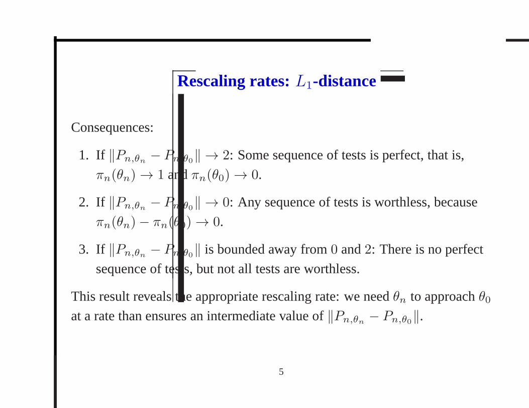
Rescaling rates:L1-distance
Consequences:
1. If ‖Pn,θn − Pn,θ0‖ → 2: Some sequence of tests is perfect, that is,
πn(θn) → 1 andπn(θ0) → 0.
2. If ‖Pn,θn − Pn,θ0‖ → 0: Any sequence of tests is worthless, because
πn(θn)− πn(θ0) → 0.
3. If ‖Pn,θn − Pn,θ0‖ is bounded away from0 and2: There is no perfect
sequence of tests, but not all tests are worthless.
This result reveals the appropriate rescaling rate: we needθn to approachθ0at a rate than ensures an intermediate value of‖Pn,θn − Pn,θ0‖.
5

Rescaling rates:L1-distance
Proof: First, for any densitiesp andq,
0 =
∫
(p− q) dµ
=
∫
p>q
(p− q) dµ+
∫
p<q
(p− q) dµ
=
∫
p>q
|p− q| dµ−∫
p<q
|p− q| dµ,
so [notice relationship with total variation distance]∫
|p− q| dµ =
∫
p>q
|p− q| dµ+
∫
p<q
|p− q| dµ
= 2
∫
p>q
|p− q| dµ.
6
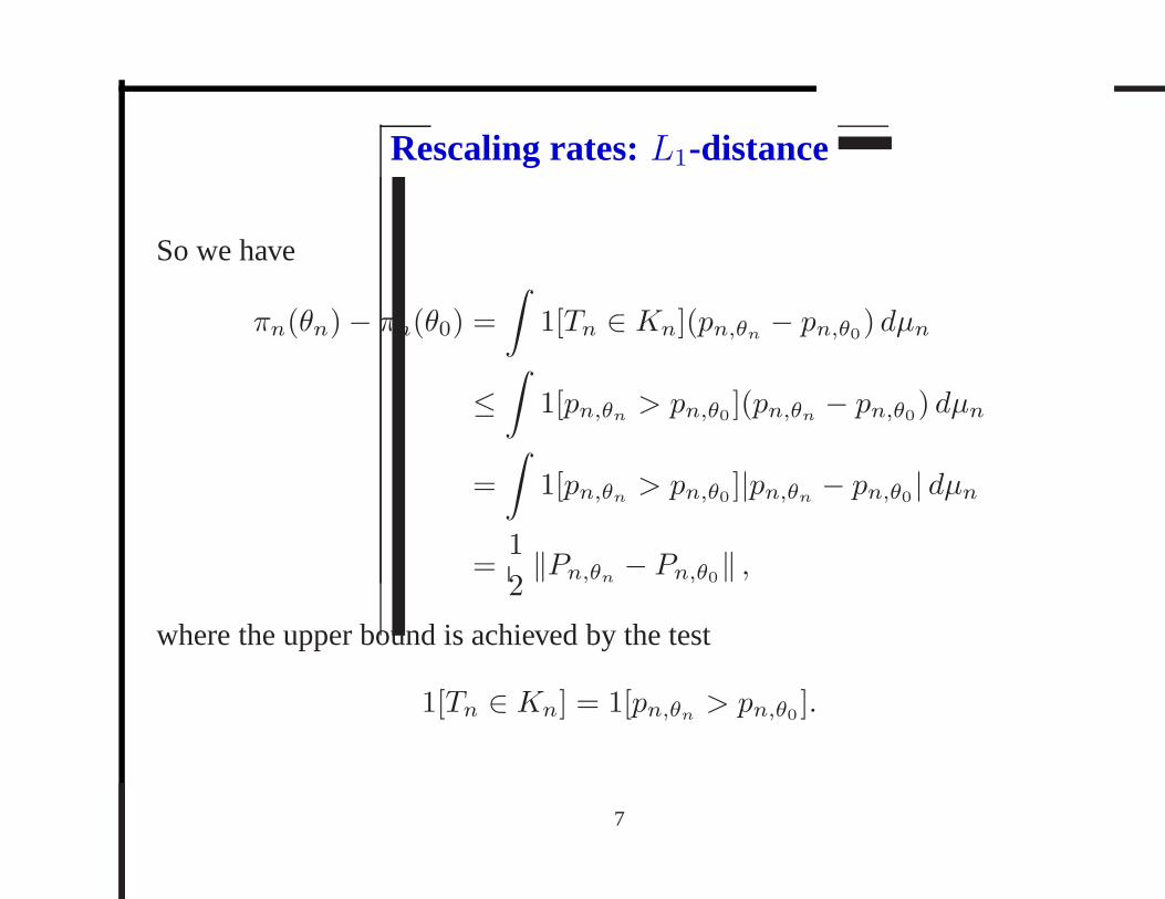
Rescaling rates:L1-distance
So we have
πn(θn)− πn(θ0) =
∫
1[Tn ∈ Kn](pn,θn − pn,θ0) dµn
≤∫
1[pn,θn > pn,θ0 ](pn,θn − pn,θ0) dµn
=
∫
1[pn,θn > pn,θ0 ]|pn,θn − pn,θ0 | dµn
=1
2‖Pn,θn − Pn,θ0‖ ,
where the upper bound is achieved by the test
1[Tn ∈ Kn] = 1[pn,θn > pn,θ0 ].
7

Rescaling rates: Hellinger distance
It’s convenient to relate theL1-distance to Hellinger distance (because then
product measures are easy to deal with).
Definition: TheHellinger distancebetweenP andQ (which have densities
p andq) is
h(P,Q) =
(
1
2
∫
(
p1/2 − q1/2)2
dµ
)1/2
.
(The1/2 ensures0 ≤ h(P,Q) ≤ 1. It is defined without it in vdV.)
8

Rescaling rates: Hellinger distance
Theorem:
nh2(Pθn , Pθ0) → ∞ ⇒ ‖Pnθn − Pn
θ0‖ → 2,
nh2(Pθn , Pθ0) → 0 ⇒ ‖Pnθn − Pn
θ0‖ → 0,
h2(Pθn , Pθ0) = Θ
(
1
n
)
⇒ ‖Pnθn − Pn
θ0‖ 6→ {0, 2}.
9

Rescaling rates: Hellinger distance
Proof:Useful properties:
2h2(P,Q) ≤ ‖P −Q‖ ≤ 2√2h(P,Q).
Also, A(Pn, Qn) = An(P,Q),
Where
A(P,Q) = 1− h2(p, q) =
∫
p1/2q1/2 dµ
is theHellinger affinity .
10

Rescaling rates: Hellinger distance
Proof (continued):
nh2(Pθn , Pθ0) → ∞
⇒ A(Pθn , Pθ0) = 1− ω
(
1
n
)
⇒ A(Pnθn , P
nθ0) → 0
⇒ h2(Pnθn , P
nθ0) → 1
⇒ ‖Pnθn − Pn
θ0‖ → 2.
11

Rescaling rates: Hellinger distance
Proof (continued):
nh2(Pθn , Pθ0) → 0
⇒ A(Pθn , Pθ0) = 1− o
(
1
n
)
⇒ A(Pnθn , P
nθ0) → 1
⇒ h2(Pnθn , P
nθ0) → 0
⇒ ‖Pnθn − Pn
θ0‖ → 0.
12

Rescaling rates: Hellinger distance
Thus, ifh2(Pθ, Pθ0) = Θ(|θ− θ0|α), then the critical quantity is the limit of
nh2(Pθn , Pθ0) = Θ((
n1/α|θn − θ0|)α)
.
If Pθ is QMD atθ0, then
h2(Pθ, Pθ0) = Θ(|θ − θ0|2),
that is,α = 2, so we consider a shrinking alternative with√n(θn − θ0) → h.
13

Rescaling rates: Hellinger distance
Definition: The root densityθ 7→ √pθ (for θ ∈ R
k) is differentiablein quadratic mean at θ if there exists a vector-valued measurable function
ℓθ : X → Rk such that, forh → 0,∫
(
√pθ+h −√
pθ −1
2hT ℓθ
√pθ
)2
dµ = o(‖h‖2).
Theorem: If Pθ is QMD atθ andIθ = Pθ ℓθ ℓTθ exists, then
h2(Pθ+h, Pθ) =1
8hT Iθh+ o(‖h‖2).
14

Rescaling rates: Hellinger distance
Proof:
2h2(Pθ+h, Pθ) =
∫
(√pθ+h −√
pθ)2
dµ
=∥
∥
√pθ+h −√
pθ∥
∥
2
L2(µ).
But QMD implies∥
∥
∥
∥
√pθ+h −√
pθ −1
2hT ℓθ
√pθ
∥
∥
∥
∥
2
L2(µ)
= o(‖h‖2),
and
∥
∥
∥
∥
1
2hT ℓθ
√pθ
∥
∥
∥
∥
2
L2(µ)
=1
4hTPθ
(
ℓθ ℓTθ
)
h
=1
4hT Iθh = O(‖h‖2).
15

Rescaling rates: Hellinger distance
So
2h2(Pθ+h, Pθ) =∥
∥
√pθ+h −√
pθ∥
∥
2
L2(µ)
=
∥
∥
∥
∥
1
2hT ℓθ
√pθ +
(
√pθ+h −√
pθ −1
2hT ℓθ
√pθ
)∥
∥
∥
∥
2
L2(µ)
=1
4hT Iθh+ o
(
‖h‖2)
+(
o(‖h‖2)O(‖h‖2))1/2
(Cauchy-Schwarz)
=1
4hT Iθh+ o
(
‖h‖2)
.
16

Rescaling rates: Hellinger distance
ConsiderPθ uniform on[0, θ]. Recall that this model is not QMD. A
straightforward calculation shows that
h2(Pθ, Pθ0) =|θ − θ0|θ ∨ θ0
.
So the appropriate shrinking alternative hasn(θn − θ0) → h.
17

Likelihood ratio tests
Suppose we observeX1, . . . , Xn, with densitypθ,
H0 : θ ∈ Θ0 versusH1 : θ ∈ Θ1.
ForΘ0 = {θ0} andΘ1 = {θ1}, the optimal test statistic is
logn∏
i=1
pθ1(Xi)
pθ0(Xi).
If we have composite hypotheses, we could instead use
Λn = logsupθ∈Θ1
∏ni=1 pθ(Xi)
supθ∈Θ0
∏ni=1 pθ(Xi)
.
18
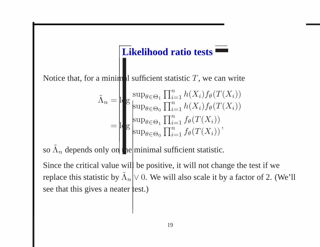
Likelihood ratio tests
Notice that, for a minimal sufficient statisticT , we can write
Λn = logsupθ∈Θ1
∏ni=1 h(Xi)fθ(T (Xi))
supθ∈Θ0
∏ni=1 h(Xi)fθ(T (Xi))
= logsupθ∈Θ1
∏ni=1 fθ(T (Xi))
supθ∈Θ0
∏ni=1 fθ(T (Xi))
,
soΛn depends only on the minimal sufficient statistic.
Since the critical value will be positive, it will not changethe test if we
replace this statistic byΛn ∨ 0. We will also scale it by a factor of 2. (We’ll
see that this gives a neater test.)
19
Likelihood ratio tests
Define
Λn = 2(Λn ∨ 0)
= 2 log
(
supθ∈Θ1
∏ni=1 pθ(Xi)
)
∨(
supθ∈Θ0
∏ni=1 pθ(Xi)
)
supθ∈Θ0
∏ni=1 pθ(Xi)
= 2 logsupθ∈Θ0∪Θ1
∏ni=1 pθ(Xi)
supθ∈Θ0
∏ni=1 pθ(Xi)
= 2n∑
i=1
(
ℓθn(Xi)− ℓθn,0(Xi)
)
,
whereθn is the maximum likelihood estimator forθ overΘ = Θ0 ∪Θ1,
andθn,0 is the maximum likelihood estimator overΘ0.
20

Likelihood ratio tests
We’ll focus on cases whereΘ = Θ0 ∪Θ1 is a subset ofRk, and whereΘ
andΘ0 are locally linear spaces. Then underH0, we’ll see thatΛn is
asymptotically chi-square distributed withm degrees of freedom, where
m = dim(Θ)− dim(Θ0). So we can get a test that is asymptotically of
levelα by comparingΛn to the upperα-quantile of a chi-square
distribution.
21