Theoretical Basis of Likelihood Methods inMolecular Phylogenetic Inference

Rhiju Das, Centre of Mathematics and Physical Sciences applied to Life scienceand EXperimental biology (CoMPLEX), University College London.

Supervisors: Z. Yang and J. Mallet, Galton Laboratory, Department of BiologyUniversity College London.

Dissertation submitted for completion of the degree of Master of Researchin University College London.

4 September, 2000

This dissertation does not exceed 18,000 words in length, exclusive of tables, figure captions,appendices, and references.

1

2

AbstractPhylogenetic inference for molecular data by the maximum-likelihood approach has beenattacked from a theoretical point of view, because the likelihood functions take differentforms for different trees, so that optimised likelihood values for different trees do notappear to be directly comparable (Nei, 1987). Here, a new "super-tree" perspective isintroduced to refute these criticisms. A super-tree likelihood expression is constructedwhich is a function of all possible bipartition lengths; it reduces to the individual treelikelihood functions when bipartitions not in a given tree are set to zero. From thisperspective, the problem of phylogeny inference is seen to be a classical statistical probleminvolving selection between composite hypotheses. In particular, the usual ML procedure iswell-justified, and, moreover, the likelihood ratio between two trees does indeed indicatethe posterior odds of the trees. This "literal" interpretation of the likelihood values isshown by simulation to provide a more intuitive indication of tree selection accuracy thanthe "integrated" likelihood posterior probabilities of Rannala and Yang (1996) andbootstrap supports. Thus, the likelihood framework for phylogenetic inference formolecular phylogenetic inference has a good theoretical basis – provided that anadequately realistic model of molecular mutation is used to fit the data. To test theadequacy of such molecular mutation models, a set of straightforward "consistency checks",based on likelihood ratio statistics, are also presented. Predicted distributions of thesestatistics are shown to agree with simulation. These consistency checks, as well as alikelihood-based tree selection procedure, have been applied to several data sets: mtDNAfrom five primates, α and β globin genes from five mammals, mtDNA and wingless genesfrom sixty Heliconiini butterflies, and mtDNA from forty mimicking races ofHeliconius melpomene and Heliconius erato butterflies. These consistency checks, as wellas the presence of internal contradictions, reject the commonly used HKY85+Γ model whenapplied to many of these data sets. It is concluded that while maximum likelihood isrigorous in principle (and preferable to theoretically unjustified methods like maximumparsimony), it should be considered a heuristic procedure for phylogenetic inference untilthe complex biological processes influencing molecular mutation are fully understood.

2

Theoretical Basis of Likelihood Methods inMolecular Phylogenetic Inference

Rhiju Das, Centre of Mathematics and Physical Sciences applied to Life science andEXperimental biology (CoMPLEX), University College London.

1. IntroductionThe inference of phylogenies based on DNA or amino acid sequences of living species hasbeen one of the most powerful techniques of modern genetics – and also one of the mostcontroversial. Molecular data has been used to find man's place among the primates(Schwartz, 1984; Hasegawa, 1991), the relationship of mammals to birds and dinosaurs(Hedges et al., 1990; Hedges, 1994), and the primordial branching pattern of the earliestliving organisms (Olsen et al., 1994b). Yet, for each problem, different researchers havepublished conflicting trees – sometimes based on the same data set!

So far, there has been no rigorous statistical framework to guide phylogenyinference. Instead, researchers depend mostly on heuristic methods, like maximumparsimony analysis (Farris et al., 1970) or the minimum evolution distance method [and itscousins, least-squares distance fitting, and neighbour-joining; see (Cavalli-Sforza andEdwards, 1967), (Fitch and Margoliash, 1967), and (Rzhetsky and Nei, 1993)]. A morerigorous technique to have gained wide popularity is the maximum likelihood (ML)method, introduced in a computationally tractable form by Felsenstein (1973, 1981). Foreach possible tree hypothesis, the likelihood of a molecular data set can be computed, usinga Markov process to model the changes among possible molecular states. The lengths of thetree branches and the parameters of the evolutionary model (like thetransition/transversion bias for DNA) are then varied until this likelihood function ismaximised, producing a single likelihood value, Ltree = exp(ltree), for each tree. Finally, the

tree with the highest log-likelihood ltree is picked as the phylogeny hypothesis bestsupported by the data. Often, the data is re-sampled with replacement, or “bootstrapped”(Felsenstein, 1985), to mimic statistical variation; if the ML method finds the same tree for,say, 95% of the bootstrap data replicates, the tree is considered well-supported.

With its likelihood/probability values and explicit description of the molecularevolutionary model, the ML method appears statistically rigorous, at first glance.However applications of the ML method to real data sets using simple evolutionary modelsof molecular mutations have often led to bizarre results. One example (among many) is theanalysis by Zardoya et al. (1998) of the whole mitochondrial genome of the lungfish, thecoelecanth, and several tetrapods to determine the closest living ancestor to the tetrapods.In their investigation, each mitochondrial gene yielded an ML tree topology (with, e.g.,lungfish+tetrapods, or coelecanth+tetrapods, as sister groups) with a likelihood severalorders of magnitude (often 105 or more) greater than alternative trees – but differentproteins favoured contradicting tree topologies.

In addition to this inconsistency in practical applications, there appear to be sometheoretical problems with the ML procedure for molecular phylogenetic inference. Aspointed out by Nei (1987), the classical likelihood theory of parameter estimation does notseem to directly apply to ML tree inference. In particular, the likelihood function has adifferent form for different trees – and the tree is not a continuous parameter (Yang et al.,1995). So it is not readily obvious that likelihoods for different trees can be properlycompared to pick out the “best” tree. Without the apparent backing of classical likelihoodtheory, the ML method for phylogeny inference instead finds its support mostly fromcomputer simulation studies and from the theoretical demonstration of its consistency(Yang, 1994b), i.e., its ability to pick out the correct tree in the limit of infinitely longmolecular sequences. Several theoretical questions remain open: How can one be sure thatthe assumed evolutionary model is properly describing all relevant aspects of the data set,including purifying/positive selection and recombination? Is the ratio of two treelikelihoods L1/L2 = exp(∆l12) an appropriate measure of the ratio of posterior

3

probabilities? Or should one take into account the variance σ(∆l12) in the log-likelihood

difference (Kishino and Hasegawa, 1989), looking at, say, exp[∆l12/σ(∆l12)] (Jermiin et al.,1997)  –  or should one trust the ratio of the trees' bootstrap supports?

The main objective of this report is to address these uncertainties lying at the heartof the ML method for molecular phylogenetic inference. In particular, it will be argued thatML is indeed statistically sound for accurate models of molecular mutation. To support thisclaim, a new “super-tree” likelihood function is introduced which is a function of allpossible bipartitions1 of the taxa. It is designed so that when all internal bipartitionsexcept for the subset found in a given tree are constrained to zero, the “super-tree”likelihood reduces to the form of the usual likelihood function defined for that tree.2 Fromthe super-tree perspective, the problem of phylogeny inference is then seen to be a classicalstatistical problem involving composite hypotheses, refuting the theoretical doubtsexpressed in (Yang et al., 1995) and elsewhere. In particular, a likelihood ratio betweendifferent tree topologies can indeed be interpreted literally as an estimate of the trees’posterior odds, “the ratio of the frequencies with which, in the long run, the twohypotheses will deliver the observed data” [section 3.4 of Edwards(1972)]  –  as long as anadequately realistic model of the molecular mutation process is used.

This last disclaimer is very important, however. The secondary objective of thisreport is to introduce some simple tests (“consistency checks”) which can check if theevolutionary model assumed in the ML analysis is realistic enough to describe a given dataset. In fact, it will be found that these tests quite often reject the most general evolutionarymodels implemented in the current generation of phylogeny inference programs. Therefore,while the ML method is, in theory, statistically well-founded, at present it is bestconsidered a heuristic method in practice, since all the biological subtleties of molecularmutation are not yet completely understood.

This report is divided into seven main sections, including this Introduction;mathematical details are collected in the appendices. In the next section, a well-definedsuper-tree likelihood function is introduced explicitly for the simplest model of binarycharacters, illustrated with several four-taxon examples, and then extended to theevolutionary models most commonly used in the literature. The third section builds on theintuition obtained from the super-tree perspective to describe how ML can be used to chooseamong tree hypotheses; in particular, likelihood ratios between trees are shown, bysimulation, to be a better indicator of the accuracy of phylogeny inference than bootstrapsupports. The fourth section develops some straightforward likelihood ratio tests to checkthe adequacy of the evolutionary model in describing a data set; several novel predictionsregarding the distributions of these likelihood ratio statistics are checked againstsimulations. The fifth section applies the ML procedure and consistency checks to severalreal data sets: a segment of mitochondrial DNA (mtDNA) from five primates; the α and βglobin genes from five mammals; mtDNA and a nuclear gene for a sixty-taxon data set ofSouth American passion-vine (Heliconiini) butterflies; and mtDNA from forty mimickingraces of Heliconius melpomene and Heliconius erato butterflies. The properties of the MLmethod, in the light of these theoretical results, simulations, and analyses of real data, arediscussed in terms of self-consistency and statistical evaluation, and compared with otherheuristic techniques of phylogeny estimation in the sixth section. The seventh sectionconcludes the report, comparing what has been achieved to what was proposed beforestarting the project.

1 In this report, the terms “bipartition” and tree “branch” are used interchangeably. The former term will be usedmore often when discussing abstract extensions to usual tree structures.2 Strimmer and Moulton (2000) have recently published another method for generalising the likelihood function fora phylogeny to a more general “phylogenetic network”. However their approach introduces several new,unspecified parameters and does not produce a unique likelihood function. Unlike the work presented here, themethod of Strimmer and Moulton does not provide a theoretical basis for the usual likelihood methods, as will bediscussed in Section 6.

4

2. The super-tree likelihood functionThis section introduces a perspective where different tree topologies are seen to be specialcases of a more general “super-tree” problem with a single likelihood function. The firstthree subsections, describing likelihood basics and the trivial two-taxon and three-taxonproblems for the simplest binary model of molecular mutation, say nothing particularly newand are intended mainly to establish notation. Subsection 2.4 introduces a super-treelikelihood function for the non-trivial four-taxon case, and briefly discusses how thisprovides a theoretical justification of the usual ML procedure of phylogeny inference. Thelast two subsections sketch how the super-tree perspective can be extended to data sets withmore taxa and with more general evolutionary models.

2.1. Likelihood basics.First, the basic formalism is described. Given a data set of m taxa aligned molecularsequences with n sites each, a general likelihood function takes the binomial form:

L =

n!n0 !n1!KnN !

p0n0 p1

n1 KpNn N , (1)

where N is the number of possible “site patterns”, the n0, n1, ... nN are the observed numbersof the site patterns in the data, and p 0, p 1, ... pN, are the probabilities of each pattern underthe given evolutionary model and tree topology. Explicitly, a site pattern is defined as a setof molecular characters that exist at a given site in the taxa. So, for example, n0 might bethe number of sites that are adenine for all the taxa in a DNA data set; n1 might be thenumber of sites that have thymine in the first taxon, but adenine in the rest; etc. If there arec possible character states, there are thus N = cm possible site patterns. Note that there is aconstraint on the observed and the predicted probabilities, that the frequencies sum to one:∑ ni/n = ∑ p i = 1.

For a given data set, the ni are constants, and the p i are varied until the likelihoodis maximised to best fit the N – 1 degrees of freedom. If the evolutionary model has enoughindependent parameters (at least N – 1 of them) one can hope to attain a “perfect” fitp i = ni/n, which is a global maximum.3

Since L is often a very small number, it is convenient to deal with logarithm of thelikelihood

l = log L = ni log pi

i=1

N

∑ , (2)

with the constant term log n!  –  ∑log[ni!] suppressed. A perfect fit gives the valuelmax = ∑nilog[ni/n].The remainder of this section describes the super-tree likelihood for the simplestevolutionary model, for binary characters with equal frequencies (Neyman, 1971). Thismodel might be appropriate for, e.g., DNA sequences where only pyrimidines and purinesare distinguished. Extensions to more realistic models of DNA and amino acid evolution aregiven in the last two sub-sections.

3 To see this, it may help the reader (especially if he/she comes from a physics background like the author) to note

that

L ∝ (npi )

nie−np i

ni!i=1

N

∏ .

The expression is simply the product of probabilities for an integer ni to be picked in a Poisson distribution withexpectation npi, and clearly has its only local maximum with respect to independent variation of the predictedfrequencies pi at ni = npi. Z. Yang (priv. comm.) has pointed out, however, that some readers would consider itobvious that a perfect fit is a global maximum of the original binomial form of L, and that this rearrangement intoPoisson form is a distraction. To each his own!

5

2.2. The simplest binary model, two-taxon case.Writing the probabilities of nucleotides to be in either of the two states, 0 or 1, as a columnvector P = [p 0, p 1]T, a simple binary evolutionary model is described by dP/dt = Q P, wherethe instantaneous rate matrix is

Q = 

−1 1 1 − 1

. (3)

The solution at any time t is

{p ij} = exp(Qt) = 

psame pdiff

pdiff psame

, (4)

where the probability that two nucleotides are different after separation time t is

pdiff =

12

[1− e −2t ], (5)

and p same = 1 – pdiff. The equilibrium character frequencies are π0 = π1 = 1/2. Now a data setof two taxa yields four site pattern numbers n00, n01, n10, and n11. Since the variables must sumto n, there are three degrees of freedom. The log-likelihood function is

l = n00 logpsame

2

+ n01 log

pdiff

2

+ n10 log

pdiff

2

+ n11 log

p same

2

= nsame log psame + ndiff log pdiff − n log 2(6)

0.0 0.1 0.2 0.3 0.4 0.50.0

0.1

0.2

0.3

0.4

0.5

0.6

0.7

0.8

0.9

1.0

fraction of sites different between two taxa

ML

est

imat

e of

div

erge

nce

tim

e

Figure 1. Maximum likelihood estimate of the divergence time between two taxa based on the simplest binary model – see equation (7).

6

So the assumption of equal character frequencies allows one to “collapse” together sitepatterns which are inverses of each other, ndiff = n01 + n10 and nsame = n00+n11. Since one has theconstraint nsame + ndiff = n, there is actually only one collapsed degree of freedom left. Thus,with a single parameter, the separation time t, one can reach the global maximum where

t (maxl) = −

12

log 1 − 2 fdiff[ ] (7)

with fdiff = ndiff/n. See Figure 1 for a plot of this function. The equation above shows that, inthis simple model, the ML estimate of the divergence time between two taxa is onlydependent on fdiff, the number of character states that are different between the two taxa.

Note that while equation (7) gives a perfect fit of the collapsed site patternfrequencies (one degree of freedom), it is not a perfect fit of the three original degrees offreedom. To accomplish that, one might consider a more general evolutionary model, with,say, fittable equilibrium frequency π0

eq ≠ 1/2 and fittable root frequency π0root

≠ 1/2. Also,note that expression (7) is not well-defined if fdiff > 1/2. If one finds such a data set, one mustset t (maxl) at the boundary t (maxl) →∞; or, more palatably perhaps, one might be able to obtaina non-boundary fit by using a more general evolutionary model.

2.3. Three-taxon case.The three-taxon case is almost as straight-forward to solve as the two-taxon case. Supposeone has three taxa A, B, and C, for which there is the single possible connecting tree shownin Figure 2.4 One needs to find the three optimum branch lengths tA, tB, and tC.For the binary model, there are eight site patterns (or 7 degrees of freedom), and as before,one can collapse them into nsame = n000 + n111; nA|BC  = n100+ n011; nB|AC  = n010 + n101; andnC|AB  = n001 + n110.

The likelihood function is then:

l = nsame log psame + nA|BC log pA|BC + nB|AC logpB|AC + nC|AB log pC|AB − n log 2 (8)

tA

A

tC

C

tB

BFigure 2. The only unrooted three-taxon tree.

4 In this and the following two subsections, one does not consider rooted trees since, with a reversible evolutionaryMarkov model and without a hypothesis like the molecular clock, ML cannot in general find the root of a tree – thepulley principle of Felsenstein (1981 ). See (Yang, 2000) for the solution of the tree-taxon rooted case under amolecular clock assumption.

7

with the pattern probabilities:

psame =14

1 + e−2 tA +tB( ) + e −2 tA + tC( ) + e −2 tB + tC( )[ ]pA|BC =

14

1− e−2 tA +tB( ) − e −2 tA+ tC( ) + e −2 tB + tC( )[ ]pB|AC = 1

41 − e−2 tA +tB( ) + e −2 tA + tC( ) − e −2 tB + tC( )[ ]

pC|AB = 14

1 + e−2 tA +tB( ) − e −2 tA + tC( ) − e −2 tB + tC( )[ ]

(9)

The above expression can be derived using the standard sum over internal character states[see, e.g., (Felsenstein, 1981)],

p same = i ={0,1}∑ π i

j={0,1}∑ p ij(tA)p ij(tB)p ij(tC), etc., (10)

or using a sum over “pathsets” as described in Appendix A. Note that the expressions in (9)are sums over exponentials; this will be a repeating theme in following subsections.

There are three collapsed degrees of freedom, and three branch parameters, so onecan again obtain a perfect fit of the collapsed site frequencies. Explicitly,

tA

(maxl) =14

− log 1− 2 fA|BC + fB|AC( )[ ] − log 1 − 2 fA|BC + fC|AB( )[ ] + log 1 − 2 fB|AC + fC|AB( )[ ]{ } , (11)

where fA|BC  = nA|BC/n, etc. Expressions for tB(maxl) and tC

(maxl) can be obtained from (11) bysymmetry.

As with the two-taxon case, some disclaimers apply. There may be a problem inobtaining the global maximum if fA|BC+fB|AC , fA|BC+fC|AB , or fB|AC+fC|AB is greater than 1/2, inwhich case the above expression is not well-defined. To find a non-boundary solution – or toobtain a perfect fit of all seven un-collapsed degrees of freedom – one might consider a moregeneral evolutionary model, say with a root frequency π0

root different from 1/2 at a chosenroot taxon, plus three different values of π0

eq(tA), π0eq(tB), and π0

eq(tC), to describe evolutionto different equilibrium frequencies on each branch.

2.4. Four-taxon case.Now, consider the four-taxon case. There are three possible trees (see Figure 3) and the non-trivial phylogenetic inference problem is to choose between them. There are eight(collapsed) site patterns that might show up in the data and they can be labelled nsame,nA|BCD, nB|ACD, nC|ABD, nD|ABC, nAB|CD, nAC|BD, and nAD|BC. Explicitly, nA|BCD is the number ofsites where taxon A has a different character than the other three taxa; the other sitepattern numbers are similarly defined. Label site pattern frequencies as before:fA|BCD = nA|BCD/n, etc. In a loose sense, one might consider the observed frequencies of sitepatterns (nA|BCD, nB|ACD, nC|ABD, nD|ABC, nAB|CD, nAC|BD, nAD|BC) as raw approximations to thebranch lengths (tA,  tB,  tC,  tD,  t I,  t II,  t III).

In the usual ML procedure, the likelihood function is different depending on theassumed tree topology. Suppose one could define a “super-tree” likelihood function, whichis dependent on all possible internal bipartition lengths, with the following property: if t II

and t III are constrained to zero, the super-tree likelihood function takes the form of the usuallikelihood function for tree I. Similarly, setting t I = t III = 0 or t I = t II = 0 yields thelikelihood functions for trees II or III, respectively. With such a super-tree likelihoodfunction, the three tree hypotheses in Figure 3 correspond to particular parameterconfigurations (five-dimensional hyper-planes) within a seven-dimensional super-treespace with a single likelihood function.

8

A

B

tA

tB

tC

tD

tI

C

D D

tA

tB

tC

tD

A

B

C

tII

DtA

tB tC

tD

A

B C

tIII

Tree I Tree II Tree IIIFigure 3. The three unrooted four-taxon tree topologies.

Before presenting the explicit form of a super-tree likelihood function, it is worthclarifying this perspective with a cartoon; see Figure 4. The contours of a putative super-tree likelihood function are plotted for a hypothetical data set; to make the diagram two-dimensional, t III is assumed to vanish (i.e., tree III is ignored as a possible topology), and ateach point in (t I,  t II) space, the likelihood has been optimised with respect to externalbranch lengths (tA,  tB, tC,  tD). The problem is to decide between tree topologies I and II;biologically realistic hypotheses correspond only to points on the positive t I and t II semi-axes. The usual ML procedure maximises the likelihood along each of these semi-axesseparately, producing parameter estimates marked “tree I” and “tree II” on Figure 4. Thetheoretical uncertainty of the usual ML procedure lies in the fact that the likelihoodfunctions maximised for tree topologies I and II appear to be different, being functions ofdifferent sets of parameters. But having a picture like Figure 4 illustrates that thelikelihood functions for different trees are indeed related – they are special cases of asingle super-tree likelihood. Thus, likelihood ratios like LI/LII are indeed directlyinterpretable as posterior odds of the two trees, given the data and the assumedevolutionary model.

tI

tII

tree I

tree II

star tree

super-tree

Figure 4. “Cartoon” of likelihood contours in the super-tree perspective. Points on the positive tI semi-axis andpositive tII semi-axis (dark lines) correspond to biologically realistic parameter sets with tree topologies I and II (seeFigure 3), respectively. The super-tree likelihood function at those points reduces to the usual ML functions forthose tree topologies.

9

Further discussion of comparisons of LI and LII to choose the tree topology is given inSection 3. Another insight from the super-tree picture is that when the likelihood ismaximised overall (t I,  t II), giving the parameters marked “super-tree” in the Figure 4, thisglobal super-tree likelihood maximum should not be too much better supported than abiologically realistic parameter set (i.e., Lsuper-tree /LI or Lsuper-tree /LII should be small). Thisobservation is the basis of a set of “consistency checks” that test the adequacy of an assumedevolutionary model in describing the data, which is further discussed in Section 4.

The super-tree likelihood function must take the same form as in the previous sub-sections:

l = ni log pi − n log2

i={site patterns}∑ (12)

So the challenge is to come up with a general form of the predicted site patternprobabilities as a function of all possible bipartition lengths (tA, tB, tC, tD, t I, t II, t III). In fact,this is fairly trivial. One starts by writing the site pattern probabilities for the individualtree topologies, which turn out to be linear combinations of a few exponentials [likeequation (9)]; see Appendix A. The following form (given in matrix form, for brevity) for thegeneralised site pattern probabilities, designed to reduce properly to the expressions for thethree separate tree topologies, is then more or less obvious:

p same

pA|BCD

pB|ACD

pC|ABD

pD|ABC

pAB|CD

pAC|BD

pAD|BD

=18

+1 +1 +1 +1 +1 +1 +1 +1+1 −1 −1 −1 +1 +1 +1 −1+1 −1 +1 +1 −1 −1 +1 −1+1 +1 −1 +1 −1 −1 −1 −1+1 +1 +1 −1 +1 −1 −1 −1+1 +1 −1 −1 −1 −1 +1 +1+1 −1 +1 −1 −1 +1 −1 +1+1 −1 −1 +1 +1 −1 −1 +1

1e−2(tA +t II +t III +tB )

e−2(tA + t I + tIII + tC )

e−2(tA + t I + tII +tD )

e−2(tB + t I + tII +tC )

e−2(tB +t I +t III +tD )

e−2(tC +t II + tIII +tD )

e−2(tA +tB +tC +tD )

(13)

See Appendix A for a more detailed discussion of the derivation of the aboveresult.5

Note that there are seven degrees of freedom, and seven independent parameters in(12) and (13). The global maximum likelihood lmax can thus be obtained when ni = npi

(barring parameters hitting a boundary; see previous sub-sections).But do equations (12) and (13) define the unique extension of L into a function of t I, t II,

and t III to reduce to the usual tree likelihood functions when all bipartitions not in a giventree are set to zero? Clearly not – one can see that special terms can be added to (13) thatdisrupt the likelihood terrain everywhere except on the hyper-planes corresponding to thethree tree hypotheses. For the simplest binary model, however, the form (13) for the sitepattern probabilities is unique in having several desirable mathematical properties[including those which make is amenable to analysis by Hadamard conjugation(Steel et al., 1998)]. In particular, the parameters (tA, tB, tC, tD, t I, t II, t III) (maxl) display a niceadditivity property. Explicitly, if one estimates the divergence time tAB between two taxaA and B based only on the fraction of sites which are different in A and B – see equation (7).

5 Interestingly, after this above result (and generalisations discussed below) was formulated, the author discoveredthat the mathematical expression had in fact been derived independently in the work on Hadamard conjugations ofHendy, Penny, Steel, Waddell, and collaborators, using a different mathematical approach (Steel et al., 1998).However, those authors have focused on heuristic (parsimony and tree-fitting) analyses of Hadamard conjugateddata patterns, outside the likelihood framework. They also have not been able to extend their Hadamard conjugationformulas to the more general evolutionary models with unequal character frequencies used in ML analyses. Thedisadvantages of these “spectral analysis” methods in comparison to the ML methods of this report, will be furtherdiscussed in Section 6.4.

10

tA

tB

tC

tD

tI

tII

tIII

A

B

C

D

Figure 5. Geometrical interpretation of the four-taxon super-tree structure.

it is easy to show that:

tAB = tA(max l) + tB

(max l) + tII(max l) + t III

(max l) , (14)

that is, the distance between the two taxa is simply the sum of the maximum likelihoodlengths of all bipartitions which might separate the two taxa in a tree. Based on thisadditivity, one might attempt to visualise a geometrical structure corresponding to thegeneral super-tree as in Figure 5, a parallelepiped of the internal bipartitions stuck withfour external branches.

The reader may protest that the super-tree likelihood of (12) and (13) isessentially a mathematical artifice, since points with non-zero t I and t II do not have a clearbiological interpretation. However, the main objective here is not to find such artificialsolutions, but to show that the likelihoods of the biologically realistic hypotheses (thepositive t I and t II semi-axes in Figure 4) are directly comparable, in that they are specialcases of a single likelihood function; and (12) and (13) accomplish this generalisation.

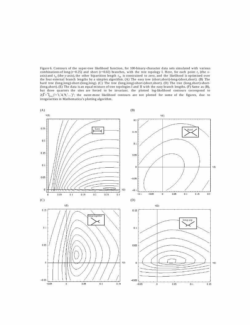
Before discussing how to obtain super-tree likelihood functions for more taxa and formore complicated evolutionary models, it is worth getting a better intuitive understandingof the super-tree space for this simplest four-taxon problem. The super-tree likelihood forsix sample data sets has been investigated. Plotted in Figures 6A-F are the likelihoodcontours in the t I–t II plane [to create these plots, t III is constrained to zero; external branchlengths are varied by a simplex algorithm (Numerical Recipes, 1992) at each (t I, t II) tooptimise the likelihood, as in Figure 6].

The first four data sets correspond to 100 character sequences simulated usingevolver from the PAML package (Yang, 1997) based on the model trees of topology I. Thefirst is an “easy” tree (long internal branch, short external branches); the second is a “hard”tree (vice versa); the third has two long branches separated by the internal branch; and thefourth has the two long branches together. The fifth data set is a mixture, where half thesites correspond to an easy tree with topology I, and half correspond to an easy tree withtopology II – mimicking the effects of a recombination event. The sixth data set has thesame simulation parameters as the hard tree (second data set), but three-quarters of thesites are forced to be invariant, so that the effects of site-rate variation can be investigated.See caption to Figure 6 for exact simulation parameters. In each figure the plotted log-likelihood contours correspond to 2(l – lmax) = 1, 4, 9, … j2, and are therefore directlycomparable between figures.

11

Figure 6. Contours of the super-tree likelihood function, for 100-binary-character data sets simulated with variouscombinations of long (t=0.25) and short (t=0.02) branches, with the tree topology I. Here, for each point tI (the x-axis) and tII (the y-axis), the other bipartition length tIII is constrained to zero, and the likelihood is optimised overthe four external branch lengths by a simplex algorithm. (A) The easy tree (short,short)-long-(short,short). (B) Thehard tree (long,long)-short-(long,long). (C) The tree (long,long)-short-(short,short). (D) The tree (long,short)-short-(long,short). (E) The data is an equal mixture of tree topologies I and II with the easy branch lengths. (F) Same as (B),but three quarters the sites are forced to be invariant. the plotted log-likelihood contours correspond to2(l –  lmax) = 1, 4, 9, … j2; the outer-most likelihood contours are not plotted for some of the figures, due toirregularities in Mathematica’s plotting algorithm.

(A)

Easy

(B)

Hard

(C)

long-together

(D)

long-sep

12

(E)

mixture

(F)

3/4 invariant

Figure 6, continued from previous page.

To begin, note that the super-tree likelihood function in each plot is quite regular,with only one local maximum, as expected. However, when constrained to the positive t I

and t II semi-axes, there can be more than one maximum – hence the observation by manyauthors that the likelihood terrain for separate tree hypotheses under the usual MLprocedure is highly irregular (see, e.g., Yang et al., 1995).

Secondly, note that in Figures 6A–D, there are always points on the positive t I

semi-axis lying within the highest one or two likelihood contours, as would beexpected – the data sets were simulated with trees of topology I. In Figure 6E, the fifthdata set, neither the t I nor the t II axes cross the highest likelihood contours, betraying thenon-”tree-like” nature of the data, which is actually a mixture of data sets simulated withtwo different trees. Figure 6F is also anomalous in that the t I and t II axes do not cross wellwithin the two highest likelihood contours. This sixth data set has been simulated withthree quarters of its sites being invariant; if one takes this site rate variation into account inthe super-tree likelihood function [see Sections 2.6 and 4(a)], the contour spacing increases tolook like Figure 6B.

Thirdly, compare the various tree-like data sets represented in Figures 6A-D. Thecontours in Figure 5B (a hard tree) are much more widely spaced than in Figure 6A (an easytree), as expected for a “harder” tree. Figure 6C (long branches separate) represents a dataset where the raw site pattern frequency fAC|BD is more than twice fAB|CD, which, if naivelytaken to indicate t II > t I, appears to favour tree topology II. This is a data set where(uncorrected) maximum parsimony (MP) would fail and would choose the wrong tree II,succumbing to MP’s infamous tendency to cluster long branches (Felsenstein, 1978). Thelikelihood function of Figure 6C, however, appropriately favours the t I axis, correspondingto the correct tree topology I. The large down-correction that the relation (13) implicitlyapplies in going from observed nAC|BD to the parameter t II leaves its imprint in the largelikelihood variance in the t II direction – compare Figure 6C to Figure 6D, simulated with adifferent tree (long branches together). In Figure 6D, the likelihood variance is largest inthe t I direction, corresponding to the large down-correction of nAB|CD.

Finally, note that the plots in Figures 6B–E (the “hard” trees) show a positivecorrelation (especially strong for the tree in Figure 6B) between t I and t II.6 A similar result

6 The normalized covariance, given by

13

was found in (Waddell et al., 1994). In fact, this is expected to be true for all “hard” cases ofphylogeny inference, where the internal branch is relatively small. This can be intuitivelyunderstood as follows. If the external branches are long, compared to the internal branch,the observed site pattern frequency corresponding to the external branches(fA|BCD, fB|ACD , fC|ABD, and fD|ABC) are larger than those corresponding to internal branches(fAB|CD, fAC|BD, and fAD|BC). Thus, the allowed variance [proportional to ni by Poissonstatistics; see footnote to Section 2.1] of the predicted site pattern numbers is larger for thosecorresponding to external bipartitions than those for internal bipartitions – that is, theexternal bipartition lengths are more free to change than the internal ones. Suppose aninternal bipartition, say t I, is forced to decrease from its maximum super-tree likelihoodvalue. The most dramatic effect of such a change will be to reduce the predicted site patternfrequency fAB|CD. Now, to optimise the likelihood, the external bipartition lengths (morefree to move than t II and t III) will increase to help restore the predicted fAB|CD; but in doingso, they will also increase the predicted fAC|BD and fAD|BC. To counter-balance this, the t II

and t III parameters will decrease (but less dramatically than the external bipartitionlengths). As a result, there is a negative correlation of the internal bipartition length t I

with its surrounding branch lengths, and a positive correlation of t I with “alternative”bipartition lengths t II and t III.

The intuition developed above, regarding regularity of the super-tree likelihood,overlap of high likelihood contours with the true tree hypothesis, and correlation betweenbipartition length parameters, will be used in Section 4 to produce statistical tests to applyto real data sets. With the simplest super-tree likelihood function (13) explicitlyintroduced, generalisations to more taxa and more complicated evolutionary models can nowbe discussed.

2.5. Generalisation to more taxa.For a general problem of phylogeny inference with m taxa, there are more parameters andmore degrees of freedom. There are (2m–5) × (2m–3) × ... ×3 possible (unrooted) treehypotheses [see, e.g., (Felsenstein, 1978)]. For the binary model which has been consideredso far, there are N = 2m possible site patterns to fit, collapsed to 2m–1 patterns if one collectstogether inverses (e.g., nABF|CDEG = n0011101 +n1100010 in a seven-taxon case), and therefore thereare 2m–1–1 collapsed degrees of freedom, due to the constraint that the site patternfrequencies must sum to one. Also, the number of bipartitions is:

12

m

2

+

m

3

+ ...+

m

m − 1

= 2m−1 − 1, (15)

which is just enough parameters to describe the collapsed degrees of freedom.A well-defined diagrammatic process for writing the super-tree likelihood function

is given in Appendix A. The form is quite similar to (13), with l = ∑ nilog p i – nlog 2, andwith each predicted site pattern probability p i taking the form of the sum of severalexponentials,

p i = 

2−(m−1) Hij exp(−ρ j )j= 1

2m

∑ . (16)

The exponents ρj correspond to “pathsets”, defined as pairs, quartets, hextets, etc. of taxa.The element ρj for a given pathset is defined as the sum of bipartition lengths that wouldseparate a single taxon of the pathset from the others. For example, for a five-taxon dataset, a pathset corresponding to pair (AB) would correspond to

∂ 2 L

∂tI∂tII

∂ 2 L

∂ 2tI

∂ 2 L

∂ 2 tII,

has been numerically evaluated at the super-tree maximum to be –0.04, +0.4,+0.04,+0.04, 0.00, and +0.1 for the datasets shown Figures 6A–F, respectively. A positive value corresponds to positive correlation between tI and tII .

14

ρ(AB)  =  tA|BCDE+tAC|BDE+tAD|BCE+tAE|BCD+tB|ACDE+tBC|ADE+tBD|ACE+tBE|ACD (17)

and a pathset corresponding to quartet (ABCD) would correspond to

ρ(ABCD)  =  tA|BCDE+tB|ACDE+tC|ABDE+tE|ABCD+tE|ABCD+tBE|ACD+tCE|ABD+tDE|ABC. (18)

Note that the total number of pathsets is

m

2

+

m

4

+ ... = 2m−1 − 1, (19)

so the number of degrees of freedom are conserved. The components of the matrix H = {Hij}are determined by assigning ±1 to each taxon depending on its character in a particular sitepattern i, and multiplying these factors for each pathset j; see the derivation inAppendix A.

There is again a simple relation like (14) between sums of internal bipartitionlengths ρ at the maximum super-tree likelihood point, and pair-wise distances t betweentaxa; indeed, ρ(AB)

(maxl) = tAB. The super-tree likelihood construction presented here is thuswell-defined, being unique if one desires this property.

Whether the general m-taxon super-tree has a simple geometrical interpretation asin Figure 5 is not clear; if such a picture does exist, it would be a complicated multi-dimensional box with m appendages sticking out. It might make an interesting problem for ageometer/topologist to characterise this beast.

The general idea of the 4-taxon case carries through here. The super-treelikelihood is quite regular, with a single local maximum, obtained by solving the perfect fitni = npi (see Section 2.1). Individual tree hypotheses correspond to particular (2m–3)-dimensional hyper-planes cutting through the 2m–1–1 dimensional space. The length of asmall internal bipartition is expected to exhibit a negative correlation with surroundingbranches, and a positive correlation with alternative internal bipartitions.

In practice, fully characterising such a large-dimensional space for a given data setis difficult. The best one might hope to do is to maximise the likelihood for several viabletree hypotheses – the usual ML procedure – and to compare those values with each otherand with the super-tree likelihood {given directly by the value ∑nilog[ni/n] – nlog 2, wherethe collapsed site pattern frequencies are perfectly fitted}. In fact, these appear to providesufficient information to select a given tree and to evaluate its statistical confidence; seeSection 3.

2.5 Generalisation to more complicated evolutionary models

(a) General mutation matrixCurrent analyses of molecular sequences with c>2 characters are more sophisticated thanthe simplest binary model discussed above:

• To model DNA changes, the 4×4 mutation matrix Q usually allows for the equilibriumfrequencies πA, πG, πC, and πT to be different from 1/4, and for there to be a biasfavouring transitions (A↔G, C↔T) over transversions (A↔C, G↔T, A↔T, C↔G),parameterised by κ [HKY85; (Hasegawa et al., 1985)].

• To model amino acid changes, the 20×20 matrix Q is fitted to data tabulated from awide range of proteins [see, e.g., (Jones et al., 1992)].

• To model codon changes, a 61×61 matrix Q (there are 43–3 codons, ignoring stop codons)can be approximately parameterised by unequal codon frequencies πAAA , πAAU , etc.; atransition/transversion ratio κ; and a non-synonymous/synonymous substitution ratioω to mimic positive (ω > 1) or purifying (ω < 1) selection (Goldman and Yang, 1994).

15

Some analyses even allow the matrix Q to change from branch to branch. Can a super-treelikelihood function be found for these models? Indeed, it can be done, although it is notnecessarily unique. Appendix A demonstrates that formulas for site pattern probabilities p i

(and thus a likelihood function) as functions of all possible bipartition lengths can beobtained; these functions reduce to the usual formulas for a given tree when bipartitions notin that tree are set to zero, as desired. For the simplest binary model, as well as for theKimura 3-substitution-type (K-3ST) model for DNA with equal base frequencies (Kimura,1980), diagrammatic procedures are given in Appendix A which produce unique super-treelikelihood functions of particularly simple forms.

There are some differences between the super-tree likelihood for the general modeland the one for the simplest binary model. For the general model, the formula for each p i isstill a linear combination of exponentials of pathset sums ρj of bipartition lengths. Unlikebefore, the coefficients of the exponentials are no longer ±1/2m–1. Also, unlike the binarymodel, for general unequal character frequencies, categories of site patterns cannot becollapsed together, as there is no longer the symmetry 0↔1. There are thus a full cm–1degrees of freedom to be fitted, with only 2m–1–1 bipartition lengths (plus possibly a fewparameters of Q) to fit them. As such, one cannot expect a perfect fit, where ni = npi, and thevalue of its likelihood at its overall maximum in super-tree space cannot be easilyestimated without direct optimisation.

Despite the complexity of the super-tree formalism for more general models, thepoint is that it can be done in principle – therefore, likelihoods for different treetopologies, as determined by the usual ML procedure, can be considered special cases of asingle likelihood function and can be directly compared.

(b) Rate variation among sitesBesides having a sophisticated rate matrix, ML analyses generally need to take intoaccount site rate variation to adequately describe real data sets. The super-tree likelihoodfunction can easily accommodate such extensions.

Consider the commonly used model where the evolutionary rates µ at different sitesare assumed to be taken from a Gamma distribution, i.e.,

dPdµ

∝ µ α− 1−1e−µ/α (Gamma distribution) (20)

Then the formulas for predicted site pattern frequencies p i must be averaged over thisdistribution. It is trivial to show that, in fact, the only necessary modification to the super-tree predicted frequencies p i is to replace all the exponentials exp(–ρi) in the formulas with(1 – α ρi)–1/α. Other rate distributions, including uniform and Inverse Gaussian distributions,or discrete distributions with, e.g., a fraction of invariant sites (finvariant), can also easily beimplemented. See, e.g., (Waddell et al., 1997).

Inclusion of site-rate-variation, however, should be considered a rather differentprocedure than changing the parameters of the rate matrix Q. For the binary model,varying the shape α of a Gamma distribution shifts the super-tree maximum likelihoodparameters, but it does not affect the super-tree maximum likelihood value,∑nilog[ni/n] – nlog 2, since, at maximum likelihood, there will always be a perfect fit of the(collapsed) site pattern probabilities. This means that an ML value for α (or any other suchsite-rate-variation parameter, like the fraction of invariant sites) cannot be solved in thesimplest binary model without invoking a particular tree hypothesis.

Note also that one must be careful about the number of parameters used to model thesite-rate distribution. Suppose, for example, one investigates a four-taxon binary data setwith the model discussed previously. If one models the site-rate-variation as aGamma distribution with shape parameter α plus a fraction finvariant of invariant sites, therewill be a problem. For each possible tree hypothesis, optimising the extra two parameters,α and finvariant, counteracts the two constraints on internal bipartitions, e.g., t II = t III = 0, andthe maximum super-tree likelihood, with perfect fit of (collapsed) site patternprobabilities, will be obtained for each tree topology. There will thus be no way todistinguish the ML values for each tree!

16

3. Comparison of tree likelihoodsHow does the super-tree perspective clarify the problem of interest – inference of thecorrect phylogeny for m molecular sequences? In the super-tree likelihood framework, thereis a continuous, well-defined likelihood function for any given set of 2m–1–1 bipartitionlengths, e.g., (tA, tB, tC, tD, t I, t II, and t III) in the four-taxon problem, and np evolutionaryparameters like character frequencies and distribution of site rates, such that the predictedsite pattern frequencies are greater than zero. The problem then is to choose between severalcomposite hypotheses, corresponding to the regions of the parameter space wherebipartition lengths not present in a given tree hypothesis are set to zero, e.g., (t I > 0;t II = t III = 0) for tree topology I in the four-taxon case.

This section describes four main ways to carry out the statistical comparison oftrees: (a) a “Bayesian” approach based on likelihood, multiplied by some prior, integratedover each tree hypothesis; (b) a more direct approach which compares likelihood valuesmaximised over each tree hypothesis (the usual ML procedure) and which interpretslikelihood ratios literally as posterior odds of trees; (c) a frequentist approach whichselects a tree based on a set of statistics like the ML values for each tree hypothesis andthen finds (by simulation) the probability of committing errors; and (d) bootstrapping,which can be interpreted as providing an approximation to any of the first threeapproaches, depending on one's prejudices. These approaches are described below in thesuper-tree likelihood framework, and then compared against computer simulations. In theend, it will be readily apparent that the second approach (b) is the most appropriate onefor phylogenetic inference, as long as the assumed molecular evolutionary model isadequately realistic. The next section will describe a series of straightforward nestedlikelihood ratio tests which are useful in checking whether one is using a fully appropriatemodel when conducting ML phylogeny inference.

(a) Bayesian decision theoryIn the Bayesian approach, the super-tree likelihood function, multiplied by a

specified prior probability, is integrated over all the branch length parameters t of a giventree hypothesis. This gives the posterior probability value for that tree topology, byBayes’ Theorem:

P(tree topology|data) =

P(tree topology)P(data|tree topology)P(data)

, (21)

where P(tree topology) is a “prior” probability for a given tree topology (usually assumedto be the same for all tree topologies); P(data) is a normalisation factor that insures thatthe sum of the posterior probabilities of all tree topologies is unity; and

P(tree topology|data) = L(t)f (t)dt∫ , (22)

where the integration is over the (2m – 3)-dimensional sub-space of the full parameterspace defined by non-zero values of bipartition lengths which are in the given tree topologyand by zero values for bipartitions not in the tree. The approach of picking the treetopology with maximum posterior probability was first proposed (although not from asuper-tree perspective) by Rannala and Yang (1996); it is sometimes called maximumintegrated likelihood (Steel and Penny, 2000). There is however a difficulty in thisapproach: one needs to define the prior probability function f(t), encoding prior knowledgeof putative branch lengths and evolutionary parameters for each tree topology. Note thatthe chosen prior must necessarily be “proper”, i.e., integrate to unity over each treehypothesis, since the likelihood function does not vanish for large branch lengths – see,e.g., the simple two-taxon case in Section 2.2. A uniform prior over all branch lengths istherefore not allowed. Rannala and Yang (1996) have used a proper prior for clock-liketrees inspired by a model of speciation/extinction as a random birth/death process. Largetand Simon (1999) have assumed a different prior, uniform on all clock-like trees with totalbranch length sums less than a large constant.

17

The main problem with the Bayesian approach appears to be computationalcomplexity. While the Markov Chain Monte Carlo algorithms of Yang and Rannala (1997)and Larget and Simon (1999) allow for the integration over a tree hypothesis to be carriedout, they are restricted to being able to explore the full tree space only for small numbers oftaxa (less than ten for the first algorithm, less than forty for the second method); also, theeffect of site-rate distributions on the analyses has not yet been investigated.

(b) Direct likelihood comparisonFollowing the approach delineated by Edwards (1972) in Chapter 3 of his treatise

Likelihood, comparing log-likelihood estimates maximised under each treehypothesis – the usual ML procedure (Felsenstein, 1981), sometimes called maximumrelative likelihood (Penny and Steel, 2000)  –  is expected to be valid, and much simpler,than the full Bayesian decision-theoretic analysis above. All tree hypotheses have thesame “simplicity”, i.e., number of fitting parameters, and the likelihoods of different treesare indeed comparable as is most clearly evident from the super-tree perspective, wherethe values are separate evaluations of a single super-tree likelihood function. Therefore,the ratios of the maximum likelihoods of two tree hypotheses provides an appropriatemeasure of their posterior odds.7 Thus, one can define a likelihood-based support8 valueP

l(tree) for a given tree hypothesis as its (maximal) likelihood divided by the sum of the(maximal) likelihoods of all the considered tree hypotheses. Previously, the likelihoodratios have generally not been interpreted so literally [for an exception, see (Strimmer andvon Haeseler, 1997)] due to the theoretical uncertainty regarding the apparent difference inthe likelihood form for different tree topologies [see (Nei, 1987), (Yang et al., 1995)]; thesuper-tree perspective of Section 2, however, mitigates this uncertainty.

The ML approach, which can be applied with a uniform prior, is expected toproduce more conservative support estimates than the full Bayesian integration describedabove as n→∞. Explicitly, the ratio of the likelihood of the ML tree to the likelihood ofany alternative tree is expected to be lower than the corresponding ratios of integratedposterior probabilities, since integration over the alternative tree parameters (which haveML internal branch lengths closer to the boundary at zero) will pick up less of the higherlikelihood regions than the best tree. Indeed, analysis of a 895-bp mitochondrial DNAdata set from six primates by Rannala and Yang (1996) show that the ∆l = ∆[log L] valuesfrom the usual ML analysis are consistently lower than the values ∆[log P(tree|data)]based on integrated posterior probabilities.

(c) Frequentist approach; critical regions.A frequentist approach is commonly assumed in the literature of phylogeny simulation.Instead of simply assigning a “degree of belief” (like a single integrated posteriorprobability or likelihood value) to each tree as in the analyses above, the idea is to find aset of the statistics, and then a tree selection procedure based on comparison of thesestatistics that minimizes the possibility of making the wrong choice.

Unfortunately the phylogeny estimation problem requires a comparison betweencomposite, non-nested hypotheses, and statistical theory offers little help in selecting a setof statistics or a selection criterion; see Chapter 23 of (Kendall and Stuart, 1961). Instead,biologists use a heuristic method; common statistics are the branch length sum S of each tree(in minimum-evolution distance methods), the total number of evolutionary changesN(steps) (in parsimony/cladistic analyses), or the values of the maximum log-likelihood lfor each tree hypothesis. The tree with the smallest value of S, N(steps), or – l is chosen asthe best tree.9

7 This is the approach in, e.g., example 3.7.1 of Edwards (1972). Note that if it is possible to reformulate a problem sothat the likelihood ratio of composite hypotheses is independent of the unspecified, “nuisance” parameters, thisshould, of course, be done [section 6.3, Edwards(1972)]. However, it does not seem possible to remove explicitdependence on the internal branch lengths from likelihood ratios in the phylogeny inference problem.8 “Support” is used here with the meaning of a “degree of belief” (in the range of 0% to 100%). It is not meant inEdwards’(1972) sense of a log-likelihood difference.9 Among the statistics listed, maximum likelihood is almost certainly the best criterion in the frequentist approach tocomposite hypotheses. In particular, it turns out that for easier problems involving comparison of simple hypotheses,as well as for very special cases involving composite hypotheses, using a likelihood criterion (possibly with a slight

18

To statistically evaluate the selection procedure, one needs to know the powerfunction, the probability of accepting the tree topology given that the true tree shares ordoes not share the same topology as the found tree – the “true positive” rate (probability ofnot making a Type I error) and the “false positive” rate (probabilities of making a Type IIerror), respectively. See, e.g., section 22.24 of (Kendall and Stuart, 1961). Simulation-basedpapers focusing on phylogeny reconstruction have been able to estimate the true positiverate, by simulating several replicates of a single known tree. However, it seems difficult toestimate a false positive rate in the general comparison between composite hypotheses. Inparticular, for phylogeny estimation, it is not known beforehand which alternative treesare expected to occur in Nature and therefore might produce a “background” signal.Therefore, the frequentist approach applied to the composite hypotheses of phylogeneticinference seems incomplete, as well as computationally burdensome.

As an example of the inappropriateness of the frequentist approach, consider thetree simulated in Figure 6D, with long branches together. It is well known that maximumparsimony (MP) is "better" (i.e., has larger true positive rate) than maximum relativelikelihood at selecting this tree from data simulated with the tree [see, e.g., (Yang,1994a)]. However, MP (but not necessarily ML) will also incorrectly select this tree if thedata was simulated with an alternative tree with the long branches separate; this is theinfamous bias of parsimony to collect together long branches, the Felsenstein zone (1978).Thus, in a loose sense, MP has higher false positive rate than ML. However, a biologistmight claim that the alternative long-branches-separate tree does not arise in Nature dueto the molecular clock constraining the shape of trees connecting four extant taxa, so thattruly the false positive rate of MP is acceptably low for biologically relevant trees. But inthat case, one could just as well include the molecular clock assumption in the ML analysis(by the appropriate constraint on branch lengths), and one expects then that both its truepositive rate and false positive rate would improve (increase and decrease, respectively)over MP. Nevertheless, in either case, it appears that the rather important step ofestimating a false positive rate is not very well-defined in the frequentist approach tostatistically evaluating tree-selection methods.

(d) BootstrappingBootstrapping describes the process of generating (pseudo)replicates of the given

data set by resampling its sites, with replacement; see, e.g., (Efron and Tibshirani, 1993).Given a tree selection procedure like maximum parsimony or maximum likelihood, thebootstrap support value Pboot(tree) for a given tree is the frequency at which is selected bythe procedure among bootstrap replicates (Felsenstein, 1985); it is very commonly used inthe current literature to statistically evaluate tree selection procedures on real moleculardata. Efron et al. (1996) have claimed that this support value is in fact a reasonableassessment of the Bayesian posterior probability of the tree, given a uniform prior and theassumption that the cut on the selection statistic would correctly separate the trees in thelimit of no statistical noise. Their analysis, however, appears to rely on a picture of acontinuous, convex parameter space divided into several contiguous regions corresponding totrees. From the super-tree perspective, one might tentatively construct such a picture bychopping up the super-tree parameter space so that, e.g., the region (t I > t II;  t I > t III)corresponds to tree topology I in the four-taxon problem. However, this is a different, andarguably incorrect, formulation of the tree selection problem from the one described above,in terms of composite hypotheses.

An alternative interpretation of the bootstrap support value is that, in being takenfrom pseudo-replicates of the correct tree, it is an estimate of the true positive rate, theprobability of not making a type I error. This appears to be the idea implemented byKishino and Hasegawa (1989) with their relative estimation of log-likelihood (RELL)technique, which estimates the distribution of likelihood ratio between the two simple(fully specified) hypotheses by bootstrapping. This interpretation has essentially beendiscounted, however, by several simulation studies; see, e.g., (Zharkikh and Li, 1992) and(Hillis and Bull, 1993). In particular, when the true positive rate is high, the bootstrap

modification to correct bias) does indeed yield a uniformly most powerful (UMP) or uniformly most powerfulunbiased (UMPU) test. See sections 22.10 and 24.24 in (Kendall and Stuart, 1961).

19

support tends to underestimate it; and when the true positive rate is low, the bootstrapsupport can give misleadingly high values for the correct or incorrect tree.

(e) Comparison of statistical approaches by simulation.This sub-section describes tree selection for four-taxon and six-taxon simulated data

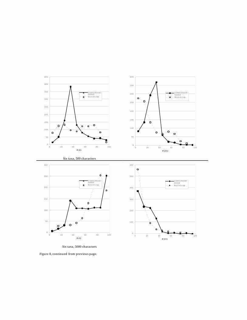
sets (1000 replicates each) for the simplest binary model. There are four main simulateddata sets, using the simplest binary model for character evolution with mutation ratesuniform across all sites, using the four-taxon (100 bases and 500 bases) and six-taxon trees(500 bases and 5000 bases) in Figure 7. A thousand replicates were simulated using PAML'sevolver and analysed using PAML's baseml. Figure 8 shows histograms of two possiblemeasures of statistical confidence – the likelihood-based support valueP

l(tree) = L tree/(LI+LII+LIII) and the bootstrap support value Pboot(tree) – for the correct treeand for an alternative tree. Note that for the six-taxon case, only trees of topology I, II, andIII in Figure 7 were assumed to be valid trees. The bootstrap supports have been computedusing the RELL technique of Kishino and Hasegawa (1989), implemented in PAML's rellapplication. For the six-taxon data sets, where the simulated tree is clock-like, Bayesianposterior probabilities (integrating the likelihood over each tree topology) have also beencalculated using PAML's mcmctree application.10 These results are shown in Figure 9, andcompared to P

l(tree) where the likelihoods have been recomputed with a molecular clockassumption.

Studying the histograms in Figure 8 yields several insights. On one hand, thebehaviour of the likelihood-based support value P

l(tree) is intuitive. For data sets withlow sequence lengths (and little phylogenetic information), the support is distributedaround 30–40% for both the correct and wrong trees. For longer sequence lengths, a largefraction of data sets are phylogenetically informative. The likelihood-based supportvalues for the correct and incorrect tree are then clustered near 90–100% and 0–10%,respectively, as expected.

A C

B DTree I Tree III

0.25 0.25

0.020.02

0.02

Tree II

C

B D

A

CB

DA

Tree "Star"

C

B D

A

0.1

1

2

3

4

5

6

7/16

1/2

1/16

1/8

5/16

9/32

1/32 1/8

5/32

5/32

1

2

4

35

6

1

2

4

35

6

1

2

4

35

6

Tree I Tree II Tree III Tree “Star”Figure 7. Four-taxon and six-taxon trees considered in the simulation studies. Tree topology I is the simulated (true)phylogeny in both sets.

10 Input parameters to the mcmctree program were as follows: empirical Bayesian analysis option; iterationaccuracy parameter δ1 = 0.5; average number of mutations per site from root to present m = 0.5 (the simulatedvalue); birth rate λ = 6.7; death rate µ = 2.5; species sampling fraction ρ = 0.06. The last three parameters are thoseused in Yang and Rannala (1997) to describe a primate data set; they describe a fairly flat prior distribution fordivergence times relative to present. It has been checked that for a dozen replicates that lowering _ _, or changing _,_, or _ does not change the posterior probabilities by more than a few percent.

20

0

50

100

150

200

250

300

350

0 20 40 60 80 100

P(I)

likelihood-basedBootstrap

0

50

100

150

200

250

300

350

0 20 40 60 80 100

P(II)

likelihood-basedBootstrap

Four taxa, 100 characters

0

50

100

150

200

250

300

350

400

0 20 40 60 80 100

P(I)

likelihood-basedBootstrap

0

100

200

300

400

500

600

0 20 40 60 80 100

P(II)

likelihood-basedBootstrap

Four taxa, 500 characters

Figure 8 (continued on next page). Comparison of likelihood-based support values Pl(tree) = Ltree/(LI+LII+LIII ) andbootstrap support values Pboot(tree) for the correct tree (I) and the wrong tree (II). Histograms are shown for thedata sets simulated with the four-taxon and six-taxon trees of Figure 7, with different sequence lengths.

21

0

50

100

150

200

250

300

350

400

450

0 20 40 60 80 100

P(I)

likelihood-basedBootstrap

0

50

100

150

200

250

300

350

400

0 20 40 60 80 100

P(II)

likelihood-basedBootstrap

Six taxa, 500 characters

0

50

100

150

200

250

300

0 20 40 60 80 100

P(I)

likelihood-basedBootstrap

0

100

200

300

400

500

600

0 20 40 60 80 100

P(II)

likelihood-basedBootstrap

Six taxa, 5000 characters

Figure 8, continued from previous page.

22

0

50

100

150

200

250

300

350

0 20 40 60 80 100P(I)

likelihood-basedBayesian

0

50

100

150

200

250

300

350

400

450

0 20 40 60 80 100

P(II)

likelihood-basedBayesian

Six taxa, 500 characters

1

10

100

1000

0 20 40 60 80 100P(I)

likelihood-basedBayesian

1

10

100

1000

0 20 40 60 80 100

P(II)

likelihood-basedBayesian

Six taxa, 5000 characters

Figure 9. Comparison of likelihood-based support values Pl(tree) = Ltree/(LI+LII+LIII ) and Bayesian integratedlikelihood posterior probabilities for the correct tree (I) and the wrong tree (II); likelihoods are calculated with amolecular clock assumption. Histograms (1000 replicates) are shown for the simulated six-taxon data sets. Note thechange to a log-scale, to better show the tails of the distributions, in the bottom plots.

number of chars. MP ML (no clock) ML (clock) MAP (clock)

500 54.0% 53.1% 69.2% 67.1%

5000 91.2% 87.1% 99.2% 96.8%

Table 1. Probability of accepting the correct tree by maximum parsimony (MP), maximum (relative) likelihood (ML)with and without a molecular clock assumption, and the maximum (integrated) likelihood MAP analyses (with clockassumption). The results are for the six-taxon tree in Figure 7, simulated with the simplest binary model (1000replicates).

23

On the other hand, the bootstrap support value Pboot(tree) has undesirableproperties. In the low-sequence-length data sets, it ranges almost uniformly from 0–100% forthe correct tree and can be misleadingly high for the wrong tree. Furthermore, for higherstatistics data sets, the bootstrap support value for the correct tree clusters near a value lessthan 100%.

The comparison for the six-taxon case of the Bayesian posterior probabilities of theMAP analysis of Yang and Rannala (1997) and the likelihood-based support values is alsointeresting. The right-hand column of Figure 9 shows that the MAP support value is morelikely to be large (> 50%) for the wrong tree than the likelihood-based support value.Also, as predicted, the Bayesian posterior probabilities are generally higher than theP

l(tree) values, even for the wrong tree.Finally, consider the “performance” of all the methods as measured by the

probability of accepting the correct tree, summarised in Table 1 for the six-taxonsimulations for maximum parsimony, for maximum likelihood (with and without molecularclock assumption), and for the MAP analysis (with molecular clock assumption). Asdiscussed above, this value, used by e.g., (Yang, 1996a) and (Penny and Steel, 2000), is onlyhalf the story in assessment of phylogenetic methods; one would also like a measure of thefalse positive rate, the probability that one has not accepted the wrong tree. Nevertheless,concentrating on the true positive rate, Table 1 shows that maximum parsimony “out-performs” the usual ML analysis without a molecular clock assumption, as would beexpected since the relevant internal branch (see tree diagram in Figure 7) is connected tolong external branches to taxon 1 and taxon 2. However, when the molecular clockassumption is made, the performance of ML improves dramatically over MP. Somewhatsurprisingly, the ML-clock analysis also outperforms the MAP analysis by a statisticallysignificant margin (based on 1000 replicates). However, this may be a result of assuming aninefficient MAP prior, and needs to be investigated further.

Based on the above results, the simplest valid procedure for phylogeny inferenceappears to be the usual ML procedure, which is to find optimal likelihoods for each treehypothesis, and to pick the one with the highest likelihood as the best. The ratio of eachtree ML value to the sum of all tree likelihood values can then be interpreted as a usefuland completely intuitive estimator of statistical support. Note, of course, that thisprocedure is only valid if the evolutionary model of the molecular sequences is correct – thenext section described a set of consistency checks which should be applied to test theadequacy of an evolutionary model in describing a data set, before any final phylogenyinferences are made.

24

4. Proposed statistical tests to check model adequacyThe previous section has argued that the usual ML procedure is statistically sound, andthat the likelihood ratios are indeed directly interpretable between different trees asposterior odds of the trees (unlike the bootstrap), if the assumed model of molecularmutation is correct. But real data sets are certainly very complex – recombination,purifying/positive selection (possibly acting differently on different taxa), andcompensating mutations, among other biological effects, may conceivably undermine thesimple molecular mutation models used in programs like PAML. This section proposes a setof “consistency checks” – likelihood ratio tests which are able, in some cases, to rejectinadequate models.

Table 2 summarises the hierarchy of nested models whose likelihoods one canevaluate for a given bipartition t I in a given data set with a given likelihood model. Thevalue lmax is defined as ∑ nilog[ni/n]. The star tree is defined by constraining t I = t II = t III = 0.Four likelihood ratio tests will described, based on the following statistics:

(a) (lsuper-tree  – lI)

(b) (lmax – lsuper-tree)

(c) (lII/III – lstar)

(d) (lmax – lI).

Statistics (a) and (c) have been chosen as indicators of how close the higher likelihoodcontours pass near parameters corresponding to the tree I topology; see, e.g., the diagram inFigure 4. Statistics (b) and (d) indicate how much worse the likelihood gets if one uses afinite set of parameters to fit the data rather than an infinite set, which would provide aperfect fit (l→lmax). The two statistics (a) and (b) require computation of lsuper-tree , which istrivial for the simplest binary model (where there is a perfect fit to the collapsed sitepattern frequencies; see Section 2.5), but for general models is rather more complicated (andpossibly not unique; see Appendix A), since it involves the optimisation of at least 2m–1

parameters. The two other statistics (c) and (d) give much the same information as the twoinvolving lsuper-tree , but are somewhat less sensitive.

Note that even more sensitive tests of unequal frequencies, site-rate-variation, etc.can be applied if one solves the maximum likelihood for a given tree under a more generalmodel and sees the change 2∆l in going to the nested, less general model [see, e.g., (Yang,1994a), (Goldman and Whelan, 2000)]. However, such tests do not give the researcher a wayto check the overall adequacy of the final, most general model considered; the likelihoodratio tests described in this section do offer such a consistency check.

Likelihoodvalue

Fitted parameters Number of parameters(simplest binary model)

Number of parameters(general model)

lmax  as many as possible (perfect fit) 2m – 1 cm – 1lsuper-tree all bipartition lengths, plus evolutionary params. 2m–1  – 1 2m–1  – 1 + nparam

lI/II/III bipartition lengths in the ML tree I (or nearest-neighbour alternatives II/III), plus evolutionaryparams.

(2m – 3) (2m – 3) + nparam

lstar bipartition lengths in a given tree with a forcedmultifurcation, plus evolutionary params.

(2m – 4) (2m – 4) + nparam

Table 2. Summary of the models considered in these reports, listed in nested order, from most general to least general.

25

Data set(model)

lsuper –  lI lsuper –  lII lsuper –  lIII lmax –  lsuper lI –  lstar lII –  lstar lIII  –  lstar lmax –  lI

4 taxa, 100characters

1.3±1.0(1.0±1.0)

1.9±1.5(>1)

2.1±1.5(>1)

4.1±1.9(4.0±2.0)

0.82±1.1(>0.25)

0.21±0.50(<0.25)

0.10±0.30(<0.25)

5.5±2.1(4.5±2.2)

4 taxa, 500characters

1.1±1.1(1.0±1.0)

3.7±2.8(>1)

3.8±2.8(>1)

4.2±2.2(4.0±2.0)

2.8±2.5(>0.25)

0.16±0.41(<0.25)

0.05±0.21(<0.25)

5.3±2.4(4.5±2.2)

6 taxa, 500characters

11.3±3.4(11.0±3.4)

11.7±3.5(>11)

11.8±3.5(>11)

17.5±4.5(16.0±4.0)

0.58±0.93(>0.25)

0.15±0.43(<0.25)

0.16±0.40(<0.25)

28.8±5.5(29.5±5.4)

6 taxa, 5000characters

10.8±3.2(11.0±3.4)

12.7±3.7(>11)

12.7±3.7(>11)

16.0±4.0(16.0±4.0)

2.0±1.9(>0.25)

0.07±0.26(<0.25)

0.08±0.29(<0.25)

26.9±5.3(29.5±5.4)

Unequal freq.(not taken intoaccount)

2.9±2.3(1.0±1.0)

5.0±3.2(>1)

6.5±3.6(>1)

145±13(4.0±2.0)

3.7±2.8(>0.25)

1.6±1.8(<0.25)

0.13±0.38(<0.25)

148±13(4.5±2.2)

Unequal freq.(taken intoaccount)

—(0.5±0.7)

—(>0.5)

—(>0.5)

—(3.5±1.9)

2.5±2.3(>0.25)

0.09±0.24(<0.25)

0.02±0.09(<0.25)

4.8±2.3(4.5±2.2)

Gamma ratevar. (not takeninto account)

6.2±3.5(1.0±1.0)

7.6±4.3(>1)

10.3±4.7(>1)

4.3±2.1(4.0±2.0)

4.7±3.5(>0.25)

3.2±2.6(<0.25)

0.57±1.00(<0.25)

10.4±4.0(5.0±2.2)

Gamma ratevariation (takeninto account)

0.6±0.8(0.5±0.7)

2.2±2.0(>0.5)

2.2±2.0(>0.5)

4.3±2.1(4.0±2.0)

1.7±1.8(>0.25)

0.06±0.21(<0.25)

0.07±0.25(<0.25)

2.8±2.3(4.5±2.2)

Table 3. Summary of mean±standard deviation (with expected values in parantheses if the assumed evolutionarymodel is correct) of (lsuper-tree –  lI/II/III), (lmax –  lsuper-tree), (lI/II/III –  lstar), and (lmax –  lI) in the simulated binary data sets(1000 replicates each). The last four rows, which show tests of the presence of unequal character frequencies andsite-rate-variation, are 4-taxa sets of 500 characters each. For the model with unequal character frequencies, thesuper-tree likelihood is not uniquely defined (see text) and difficult to evaluate without direct optimisation; so thoseentries are not evaluated.

The expected asymptotic distributions of these statistics is discussed below, and arechecked against computer simulations. The four main simulated data sets have beendescribed in the previous section. Histograms of likelihood ratio statistics from these runsare shown in Figures 10–12. In addition, one data set of 1000 replicates of 500 bases each,with the four-taxon tree, was simulated with unequal character frequencies (π0 = 0.8,π1 = 0.2); and one data set (also 1000 replicates, 500 bases) was simulated with site-rate-variation described by a Gamma distribution with α = 0.5, but with equal characterfrequencies. Summary likelihood ratio statistics for all of the simulations are given inTable 3.

26

(a) The statistic (lsuper-tree  – lI)One of the main observations of Section 2.4 was that for simulated data sets based

on a single tree topology, a point in super-tree space corresponding to the correct treetopology was always enclosed by one of the high-likelihood contours. More quantitatively,for large n, one expects the statistic 2(lmax – lI) to be distributed as χ2

k, where k is thedifference in the number of parameters of the full model and the nested model [chapter 24 in(Kendall and Stuart, 1961)]. Explicitly,

dPdl ∝ l k/2−1e−l , (χ2

k distribution) (23)

with the proportionality constant determined by normalising the distribution to have unitintegral. In this case,

k = (# super-tree parameters)  –  (# tree parameters) = (2m–1 –1)  –  (2m – 3),

which equals 2 (m = 4), 8 (m = 5), 22 (m = 6) etc., in the asymptotic limit n→∞. If, in a givendata set with a given evolutionary model, the best tree hypothesis yields a (lsuper-tree  – lI)larger than a critical value, as determined by a χ2 test at some specified significance level,one can reject the assumed evolutionary model. Note that in using the likelihood lI of theML tree hypothesis rather than some guess of the “true tree” (which may be unknown), thetest is checking a “best-case” scenario – if the ML tree is rejected by the (lsuper-tree  – lI) testthan so will any other tree.

The histograms of Figure 10 show the actual (lsuper-tree  – lI) distributions for foursimulated data sets fitted to χ2

k distributions. The four-taxon data sets fit11 to k ≈ 2.6 (100bases) and k = 2.1 (500 bases), which are close to the expected limit k = 2. In particular,while the fits are not perfect for the lowest values of (lsuper-tree  – lI), they are excellent forthe right-hand tail of the distribution, which is the crucial part for carrying out confidencetests. The six-taxon data sets fit well through the whole range of (lsuper-tree  – lI), withk = 22.6 (500 bases) and k = 21.6 (5000 bases), quite close to the expected k = 22.

To illustrate the power of the test, consider the results of a more complex datasimulations with unequal character frequencies, and with site-rate-variationparameterised by a Γ distribution (α = 0.5), summarised in Table 3. When the unequalfrequencies are not taken into account [i.e., when one forces π0 = π1 = 1/2] in the former dataset, the (lsuper-tree  – lI) statistic is found to be 2.9±2.3 (mean ± standard deviation), with1.0±1.0 being the expected value. And when, in the latter data set, the site-rate-variationis ignored and then taken into account, (lsuper-tree  – lI) decreases dramatically from 6.2±3.5(expected: 1.0±1.0) to 0.6±0.8 (expected: 0.5±0.7). Thus, in the majority of data sets, if onefails to take into account either unequal frequencies or site-rate-variation, checking(lsuper–tree  – lI) will provide a necessary warning, especially in the latter case.

11 Fits of the χ2

k distribution to simulations here (and later) are accomplished by setting k/2 equal to the mean of thelog-likelihood-difference found in the simulation.

27

0

20

40

60

80

100

120

140

160

180

200

0 2 4 6 8 10

LnL(super) - LnL(I)

0

50

100

150

200

250

0 2 4 6 8 10

LnL(super) - LnL(I)

Four taxa, 100 characters Four taxa, 500 characters

0

20

40

60

80

100

120

140

0 5 10 15 20 25 30

LnL(super) - LnL(I)

0

20

40

60

80

100

120

140

160

0 5 10 15 20 25 30

LnL(super) - LnL(I)

Six taxa, 500 characters Six taxa, 5000 characters

Figure 10. Distributions of the (lsuper-tree –  lI) statistic compared to predicted distributions of the form χ2k for

simulations (1000 replicates) of the simplest binary model for the four-taxon and six-taxon trees shown in Figure 7.Fitted values of the parameter k are given in the text.

28

(b) The statistic (lmax – lsuper-tree)A second way to check the description of the evolutionary process is by looking at

the statistic (lmax – lsuper- tree).12 In the limit n→∞, 2(lmax – lsuper-tree) is expected to follow a χ2k

distribution with

k = (# site patterns)  –  (# super-tree parameters) = (cm–1)  –  (2m–1–1) = cm–2m–1

(where c is the number of possible character states). For finite n, not all site patterns showup in the data, and k is usually different from than the asymptotic limit but can still beestimated fairly easily; see the discussion of (lmax – lI) in (d) below.

The histograms of Figure 11 show the (lmax – lsuper-tree) distributions for four simulateddata sets fitted to χ2

k distributions. The four taxa data sets fit well with k = 8.2 (100bases)and k = 8.4 (500 bases), with the expected asymptotic limit being k = 8. The six-taxon datasets fit well to k = 34 (500 bases) and k = 32 (5000 bases), with expected asymptotic limitbeing k = 32.

The (lmax – lsuper-tree)statistic, like (lsuper-tree  – lI) above, provides a particularly goodconsistency check on data sets which have unequal frequencies; see Table 3. For thesimulated data set with (π0 = 0.8, π1 = 0.2), not taking into account the unequal frequenciesyields (lmax – lsuper-tree) = 145±13, much larger than the expected value being 4.5±2.2. Note

that this statistic cannot provide a sensitive test for site-rate-variation, since lsuper-tre e doesnot vary with, e.g., the shape parameter of an assumed Γ distribution of site rates. Indeed,for the simulated data set with site-rate-variation, (lmax – lsuper-tree) = 4.8±2.3, with theexpected value, 4.5±2.2.

Thus the (lmax – lsuper-tree) statistic is especially good at catching inconsistencies inunequal frequencies, and, presumably more generally, other parameters of the mutationmatrix. The other (lsuper-tree  – lI) statistic described above should be used to check site-rate-variation.

12 The reader may wonder why this statistic doesn’t vanish for the simplest binary model, where one can attain a“perfect fit”. The answer is that the super-tree can perfectly fit the collapsed degrees of freedom – but in collapsingpairs of site patterns which are inverses of each other (under the switch 0↔1), an assumption has been made thatthe inverses in each pair occur with equal probabilities. Testing (lmax – lsuper-tree) checks this assumption.

29

0

20

40

60

80

100

120

140

0 5 10 15 20

LnL(max)-LnL(super)

0

20

40

60

80

100

120

140

0 5 10 15 20

LnL(max)-LnL(super)

Four taxa, 100 characters Four taxa, 500 characters

0

20

40

60

80

100

120

0 10 20 30 40

LnL(max)-LnL(super)

0

20

40

60

80

100

120

0 10 20 30 40

LnL(max)-LnL(super)

Six taxa, 500 characters Six taxa, 5000 characters

Figure 11. Distributions of the (lmax– lsuper-tree) statistic compared to predicted distributions of the form χ2k for

simulations (1000 replicates) of the simplest binary model for the four-taxon and six-taxon trees shown in Figure 7.Fitted values of the parameter k are given in the text.

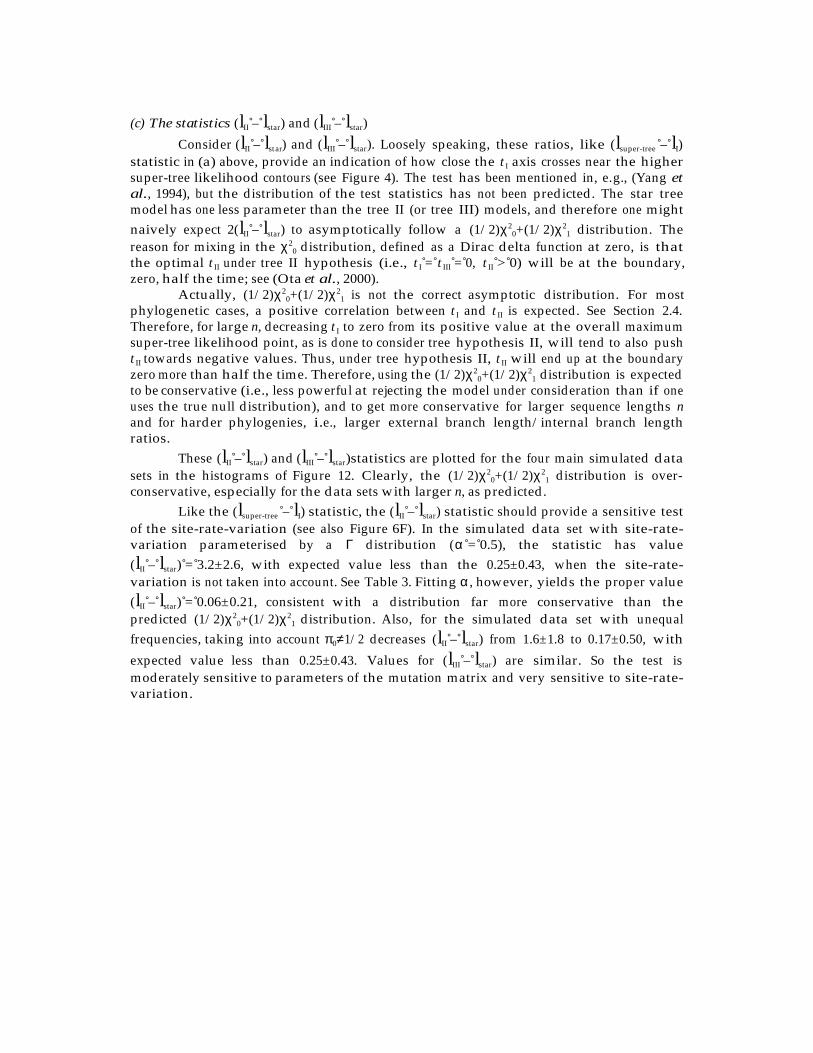
30

(c) The statistics (lII – lstar) and (lIII – lstar)

Consider (lII – lstar) and (lIII – lstar). Loosely speaking, these ratios, like (lsuper-tree  – lI)statistic in (a) above, provide an indication of how close the t I axis crosses near the highersuper-tree likelihood contours (see Figure 4). The test has been mentioned in, e.g., (Yang etal., 1994), but the distribution of the test statistics has not been predicted. The star treemodel has one less parameter than the tree II (or tree III) models, and therefore one mightnaively expect 2(lII – lstar) to asymptotically follow a (1/2)χ2

0+(1/2)χ21 distribution. The

reason for mixing in the χ20 distribution, defined as a Dirac delta function at zero, is that

the optimal t II under tree II hypothesis (i.e., t I = t III = 0, t II > 0) will be at the boundary,zero, half the time; see (Ota et al., 2000).

Actually, (1/2)χ20+(1/2)χ2

1 is not the correct asymptotic distribution. For mostphylogenetic cases, a positive correlation between t I and t II is expected. See Section 2.4.Therefore, for large n, decreasing t I to zero from its positive value at the overall maximumsuper-tree likelihood point, as is done to consider tree hypothesis II, will tend to also pusht II towards negative values. Thus, under tree hypothesis II, t II will end up at the boundaryzero more than half the time. Therefore, using the (1/2)χ2

0+(1/2)χ21 distribution is expected

to be conservative (i.e., less powerful at rejecting the model under consideration than if oneuses the true null distribution), and to get more conservative for larger sequence lengths nand for harder phylogenies, i.e., larger external branch length/internal branch lengthratios.

These (lII – lstar) and (lIII – lstar)statistics are plotted for the four main simulated datasets in the histograms of Figure 12. Clearly, the (1/2)χ2

0+(1/2)χ21 distribution is over-

conservative, especially for the data sets with larger n, as predicted.Like the (lsuper-tree  – lI) statistic, the (lII – lstar) statistic should provide a sensitive test

of the site-rate-variation (see also Figure 6F). In the simulated data set with site-rate-variation parameterised by a Γ distribution (α = 0.5), the statistic has value(lII – lstar) = 3.2±2.6, with expected value less than the 0.25±0.43, when the site-rate-variation is not taken into account. See Table 3. Fitting α, however, yields the proper value(lII – lstar) = 0.06±0.21, consistent with a distribution far more conservative than thepredicted (1/2)χ2

0+(1/2)χ21 distribution. Also, for the simulated data set with unequal

frequencies, taking into account π0≠1/2 decreases (lII – lstar) from 1.6±1.8 to 0.17±0.50, with

expected value less than 0.25±0.43. Values for (lIII – lstar) are similar. So the test ismoderately sensitive to parameters of the mutation matrix and very sensitive to site-rate-variation.

31

0

50

100

150

200

250

300

350

0 2 4 6 8 10

LnL(II/III)-LnL(star)

0

50

100

150

200

250

300

350

0 2 4 6 8 10

LnL(II/III)-LnL(star)

Four taxa, 100 characters Four taxa, 500 characters

0

50

100

150

200

250

300

350

0 2 4 6 8 10

LnL(II/III)-LnL(star)

0

50

100

150

200

250

300

350

0 2 4 6 8 10

LnL(II/III)-LnL(star)

Six taxa, 500 characters Six taxa, 5000 characters

Figure 12. Distributions of the (lII –  lstar) (squares) and (lIII  –  lstar) (squares) statistics compared to predicted(1/2)χ2

0+(1/2)χ21 distribution for simulations (1000 replicates) of the simplest binary model for the four-taxon

and six-taxon trees shown in Figure 7. In these histograms, the bin at zero is not shown, as its value is an order-of-magnitude higher than for any other bins; for each of the four data sets, more than half of the 1000 replicates yielded(lII –  lstar)=0 or (lIII  –  lstar)=0.

32

(d) The statistic (lmax – lI)

The (lmax – lI) provides a test that combines the (lsuper-tree  – lI) and (lmax – lsuper-tree)discussed in (a) and (b) above; it is expected to be less sensitive than conducting tests (a) and(b) separately, but is more straightforward to carry out for general evolutionary modelswhere lsuper-tree is difficult to find or not unique. In the asymptotic limit, 2(lmax – lI) is expectedto follow a χ2

k distribution with

k = (# site patterns) – (# tree parameters) = (cm–1) – np,

where np is the number of optimised model parameters, including branch lengths, characterfrequencies, etc. This test statistic has been described before in e.g., (Navidi et al., 1991),(Reeves, 1992), (Goldman, 1993), and (Yang, 1994b), but its predicted distribution dependedon either assuming the infinite-sequence-length limit or conducting numerically intensivesimulation.

For finite sequence length n, however, the distribution will not be this χ2k

distribution, since all site patterns will generally not show up in the data – in fact, it iscommon to see data sets where the vast majority (sometimes >90%) of sites are “constant”,the same for all taxa. Yang et al. (1995) have attempted a strategy of combining into largercategories those data points (site patterns) which have similar low probabilities, and thenchecking the data against prediction with a likelihood ratio or Pearson X2 statistic.However, the method of Yang et al. (1995) seems to involve some bias in determining whichsite patterns to combine; so, in this report, the (lmax – lI) statistic (without such re-groupingof the data) is used.

To approximate the distribution of this statistic, note that the mean (lmax – lI) isexpected to be rather large (exponentially growing with the number of taxa), and it istherefore valid to approximate its distribution as a normal distribution, by the Law ofLarge Numbers. The mean and variance of the normal distribution of (lmax – lI) can in fact beeasily estimated by a procedure described in Appendix B, based on summing contributionsfrom Poisson distributions for individual site patterns.

For the simulated data sets, the predicted (lmax – lI) distribution will simply be the

convolution of the (lmax – lsuper-tree) and (lsuper-tree  – lI) distributions, so the fit of the simulatedstatistic to the predicted asymptotic distribution, as well as the sensitivity to parametersof the mutation matrix, follows directly from the discussion above. See also the last columnof Table 3.

0

50

100

150

200

250

300

10 100 1000 10000

number of bases

predicted

TREE I

TREE IITREE III

Figure 13. Comparison of predicted mean (lmax – lI) to actual (lmax – lI/II/III) from 1000 simulated replicates, as afunction of the number of bases in the sequence. Data is simulated with the four-taxon tree of Figure 7, and the JC69model for nucleotides. See also Table 4.

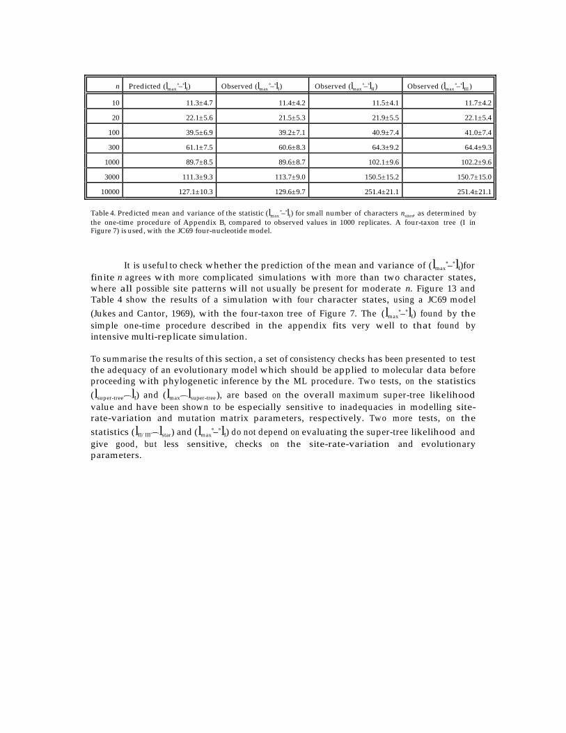
33

n Predicted (lmax – lI) Observed (lmax – lI) Observed (lmax – lII) Observed (lmax – lIII )

10 11.3±4.7 11.4±4.2 11.5±4.1 11.7±4.2

20 22.1±5.6 21.5±5.3 21.9±5.5 22.1±5.4

100 39.5±6.9 39.2±7.1 40.9±7.4 41.0±7.4

300 61.1±7.5 60.6±8.3 64.3±9.2 64.4±9.3

1000 89.7±8.5 89.6±8.7 102.1±9.6 102.2±9.6

3000 111.3±9.3 113.7±9.0 150.5±15.2 150.7±15.0

10000 127.1±10.3 129.6±9.7 251.4±21.1 251.4±21.1

Table 4. Predicted mean and variance of the statistic (lmax – lI) for small number of characters nsites, as determined bythe one-time procedure of Appendix B, compared to observed values in 1000 replicates. A four-taxon tree (I inFigure 7) is used, with the JC69 four-nucleotide model.

It is useful to check whether the prediction of the mean and variance of (lmax – lI)forfinite n agrees with more complicated simulations with more than two character states,where all possible site patterns will not usually be present for moderate n. Figure 13 andTable 4 show the results of a simulation with four character states, using a JC69 model(Jukes and Cantor, 1969), with the four-taxon tree of Figure 7. The (lmax – lI) found by thesimple one-time procedure described in the appendix fits very well to that found byintensive multi-replicate simulation.

To summarise the results of this section, a set of consistency checks has been presented to testthe adequacy of an evolutionary model which should be applied to molecular data beforeproceeding with phylogenetic inference by the ML procedure. Two tests, on the statistics(lsuper-tree – lI) and (lmax – lsuper-tree), are based on the overall maximum super-tree likelihoodvalue and have been shown to be especially sensitive to inadequacies in modelling site-rate-variation and mutation matrix parameters, respectively. Two more tests, on thestatistics (lII/III – lstar) and (lmax – lI) do not depend on evaluating the super-tree likelihood andgive good, but less sensitive, checks on the site-rate-variation and evolutionaryparameters.

34

5. Real data setsBefore discussing the theoretical results introduced above, it is worth looking at some realdata sets. Does ML analysis using common evolutionary models on real DNA data pass the“consistency checks” described in Section 4? Are the resulting likelihood-ratio-basedsupports reasonable? This section applies ML analysis to phylogeny inference in four datasets: a mitochondrial DNA (mtDNA) segment from five primates; α and β globin genes fromfive mammals; mtDNA and the wingless gene from almost sixty species (the generaHeliconius and Eueides, and outgroups) of passion-vine butterflies; and mtDNA fromseveral mimicking races of Heliconius erato and Heliconius melpomene butterflies.

5.1. Mitochondrial DNA from five primates.This data set is a “classic” in molecular phylogenetic studies, having been previouslyanalysed by several authors, e.g., Yang et al. (1994b), and it is included with the PAMLpackage. The data consists of an aligned 895-bp segment of DNA (including a tRNA geneand parts of two protein-coding genes) from human, chimpanzee, gorilla, orangutan, andgibbon (Brown et al., 1982). The tRNA bases, and the first, second, and third codon positionsare considered separate site categories, and are analysed as separate data sets. The threetrees (plus a star tree) of Figure 14 are tested.

Before comparing likelihoods of the trees, the consistency checks described inSection 3.1 must be applied. Since estimating the value of lsuper-tree is difficult in this six-

taxon case, only the (lmax– lI) and (lII/III– lstar) tests have been performed. A succession ofevolutionary models are tested, starting with the simplest JC69 model (equal basefrequencies; no transition/transversion bias κ; no site-rate-variation), then F81 [allowingfor unequal base frequencies, measured empirically; (Felsenstein, 1981)], then HKY85(allowing for unequal base frequencies and a fitted κ ≠1), and finally the more generalHKY85+Γ and HKY85+3cat (modelling the site-rate distribution as a Gamma distributionwith fitted shape parameter α, and as three discrete categories with fitted frequencies andrates, respectively).

To illustrate the tests, lI, lII, lIII, and lstar are shown in Table 5 for the third codonposition bases, which might be expected to be a relatively “neutral” marker, sincesubstitutions at the third codon positions are usually synonymous. Models JC69 and F81 areeasily rejected (with 95% confidence) by the (lmax– lI) test, where the distribution of thisstatistic is approximated as a normal distribution with mean and variance as estimated inAppendix B; the HKY85 models (with and without site-rate-variation) cannot be rejectedat 90% confidence by this test. Furthermore, the HKY85 and HKY85+3cat models are alsorejected with 95% confidence by the (lII – lstar) test, whose null distribution is(conservatively) taken to follow the (1/2)χ2

0+(1/2)χ21 distribution. Apparently site-rate-

variation must be taken into account – and with an appropriately shaped distribution. Theresults for the other codon positions and the tRNA bases are similar to the results at thethird codon position, except the (lII– lstar) test is not able to reject any of the models for theslow-mutating second codon position bases.

Tree I Tree II Tree III Tree Star

Figure 14. Possible unrooted phylogenies considered in five-primate mitochondrial DNA set.

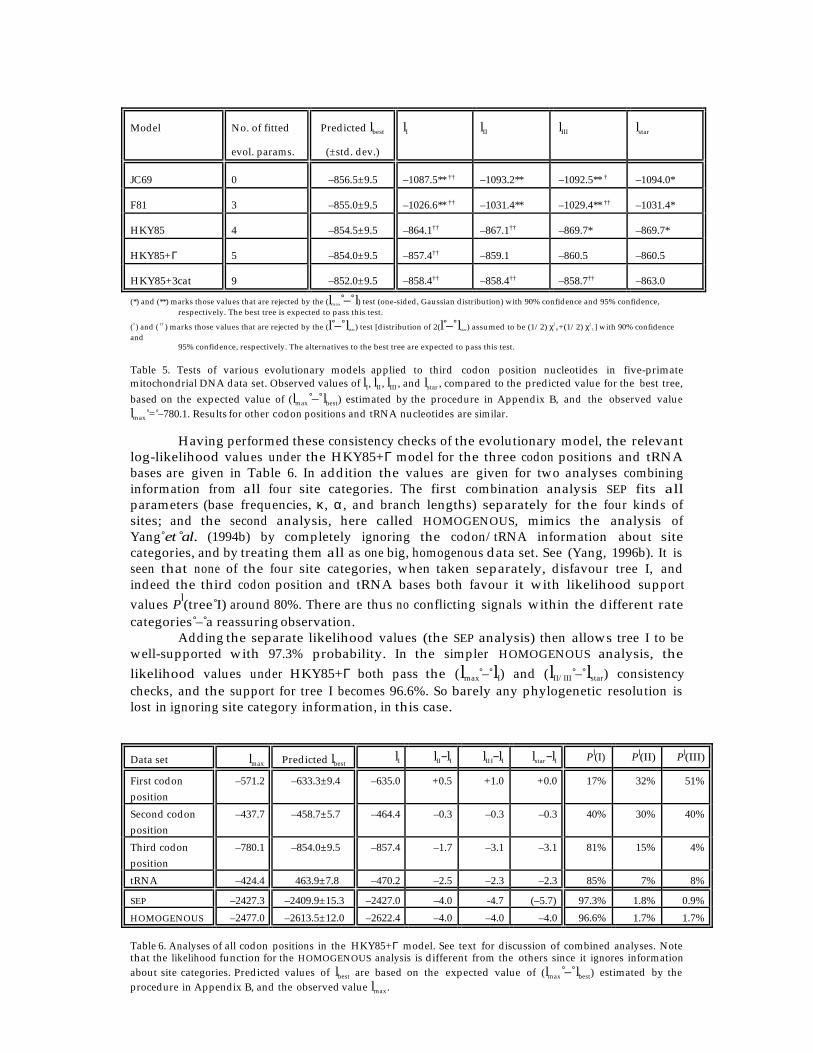
35

Model No. of fitted

evol. params.

Predicted lbest

(±std. dev.)

lI lII lIII lstar

JC69 0 –856.5±9.5 –1087.5** †† –1093.2** –1092.5** † –1094.0*

F81 3 –855.0±9.5 –1026.6** †† –1031.4** –1029.4** †† –1031.4*

HKY85 4 –854.5±9.5 –864.1†† –867.1†† –869.7* –869.7*

HKY85+Γ 5 –854.0±9.5 –857.4†† –859.1 –860.5 –860.5

HKY85+3cat 9 –852.0±9.5 –858.4†† –858.4†† –858.7†† –863.0

(*) and (**) marks those values that are rejected by the (lmax –  l) test (one-sided, Gaussian distribution) with 90% confidence and 95% confidence,respectively. The best tree is expected to pass this test.

(†) and ( †† ) marks those values that are rejected by the (l –  lstar) test [distribution of 2(l –  lstar) assumed to be (1/2) χ20+(1/2) χ2

1] with 90% confidenceand

95% confidence, respectively. The alternatives to the best tree are expected to pass this test.

Table 5. Tests of various evolutionary models applied to third codon position nucleotides in five-primatemitochondrial DNA data set. Observed values of lI, lII , lIII , and lstar , compared to the predicted value for the best tree,based on the expected value of (lmax –  lbest) estimated by the procedure in Appendix B, and the observed valuelmax = –780.1. Results for other codon positions and tRNA nucleotides are similar.

Having performed these consistency checks of the evolutionary model, the relevantlog-likelihood values under the HKY85+Γ model for the three codon positions and tRNAbases are given in Table 6. In addition the values are given for two analyses combininginformation from all four site categories. The first combination analysis SEP fits allparameters (base frequencies, κ, α, and branch lengths) separately for the four kinds ofsites; and the second analysis, here called HOMOGENOUS, mimics the analysis ofYang et al. (1994b) by completely ignoring the codon/tRNA information about sitecategories, and by treating them all as one big, homogenous data set. See (Yang, 1996b). It isseen that none of the four site categories, when taken separately, disfavour tree I, andindeed the third codon position and tRNA bases both favour it with likelihood supportvalues Pl(tree I) around 80%. There are thus no conflicting signals within the different ratecategories – a reassuring observation.

Adding the separate likelihood values (the SEP analysis) then allows tree I to bewell-supported with 97.3% probability. In the simpler HOMOGENOUS analysis, thelikelihood values under HKY85+Γ both pass the (lmax – lI) and (lII/III – lstar) consistencychecks, and the support for tree I becomes 96.6%. So barely any phylogenetic resolution islost in ignoring site category information, in this case.

Data set lmax Predicted lbestlI lII–lI lII I–lI lstar–lI Pl(I) Pl(II) Pl(III)

First codonposition

–571.2 –633.3±9.4 –635.0 +0.5 +1.0 +0.0 17% 32% 51%

Second codonposition

–437.7 –458.7±5.7 –464.4 –0.3 –0.3 –0.3 40% 30% 40%

Third codonposition

–780.1 –854.0±9.5 –857.4 –1.7 –3.1 –3.1 81% 15% 4%

tRNA –424.4 463.9±7.8 –470.2 –2.5 –2.3 –2.3 85% 7% 8%

SEP –2427.3 –2409.9±15.3 –2427.0 –4.0 -4.7 (–5.7) 97.3% 1.8% 0.9%

HOMOGENOUS –2477.0 –2613.5±12.0 –2622.4 –4.0 –4.0 –4.0 96.6% 1.7% 1.7%

Table 6. Analyses of all codon positions in the HKY85+Γ model. See text for discussion of combined analyses. Notethat the likelihood function for the HOMOGENOUS analysis is different from the others since it ignores informationabout site categories. Predicted values of lbest are based on the expected value of (lmax –  lbest) estimated by theprocedure in Appendix B, and the observed value lmax.

36

5.2. α/β-globin codons from six mammals.A second data set analysed here is the combined α- and β- globin codon sequences fromhuman, goat(α)/cow(β), rabbit, rat, and marsupial included with the PAML package.These globin genes are, of course, textbook examples in most fields of molecular biology, fromstructural genomics (Branden and Tooze, 1999) to biochemistry (Stryer, 1995). Inphylogenetics, they have played an important role is the search for positive selection ingenes (Yang et al., 2000) and in controversies of the relation of birds to reptiles andmammals (Hedges, 1994).The data set has been analysed in several ways: as one large DNA sets, with the HKY85+Γmodel; at each codon position separately as three DNA data sets (HKY85+Γ); as an aminoacid data set [with empirical transition matrices JTT, Dayhoff, mtREV24, and mtMAMincluded in the PAML package, modified to reflect the codon frequencies empiricallydetermined from this data set]; and as a codon data set to be analysed with a modelincluding various distributions for a non-synonymous/synonymous ratio parameter. Thereare fifteen (unrooted) bifurcating trees; Table 7 shows the results for the log-likelihoodvalues of the eight trees of Figure 15, for each of these analyses. Apparently Tree III' isfavoured by most of the analyses; but the true tree is known to be Tree I [see, e.g., (Janke etal., 1997)]. However, none of the analyses pass the basic consistency checks, despite thegenerality of some of these models. That is, the best tree in any of these analyses is rejectedby the (lmax – lI) test, indicating that the models are not complex enough to adequatelydescribe the data. See Section 5.2 for further discussion. What would happen if one ignored the rejection of the model by the consistencychecks and still analysed this data set using, e.g., the amino acids with the best-fitting JTTmatrix? The marsupial branch would be more favoured to attach to the goat branch than tothe correct rat branch by a factor of almost 100, based on likelihood-based support values,and by a factor of 5, based on RELL bootstrap support values. Thus, dangerously misleadingphylogeny inferences can be made if one fails to test if the evolutionary model can berejected by the (lmax– lI) and (lalternative– lstar) consistency checks.

Tree I Tree II Tree III Tree Star

Tree I' Tree II' Tree III' Tree Star'

Figure 15. Eight (out of fifteen) possible unrooted phylogenies for which illustrative log-likelihood values arepresented (see Table 4), for the five-mammal α/β-globin data set.

37

Data set lmax Pred. lbestlI lII lIII lstar lI' lII' lIII' lstar'

DNA:

(nocategorisation)

–2872.8 –3124.2±15.0 -3148.2**†† -3148.7**† -3149.3** -3150.7** -3149.3**†† -3150.2**† -3151.7** -3151.8**

DNA:

1st codonposition

–790.8 –909.8±12.7 -934.3**†† -936.1**  -935.7** -936.2** -935.6** -935.6**  -935.1**  -935.6**

2nd codonposition

–685.8 –786.2±12.2 -810.7**  -810.9**  -808.6** -810.9** -807.5**†† -809.9**  -809.7**  -809.9**

3rd codonposition

–1059.6 –1206.9±13.1 -1250.5**  -1248.6**†† -1250.5** -1250.5** -1252.0** -1250.1**†† -1252.0**  -1252.0**

Amino acids:

JTT –1189.1 –1655.2±35.1 -1743.4**†† -1740.9**†† -1743.9**†† -1746.1** -1733.0**†† -1738.2**†† -1739.9**†† -1742.5**

JTT+_ –1189.1 –1654.7±35.1 -1720.1**† -1719.1**†† -1720.8** -1721.7** -1711.2**†† -1716.9**†† -1717.7**  -1718.2**

JTT+__ +empF –1189.1 –1645.2±35.1 -1694.7**†† -1695.2**†† -1696.5** -1697.5** -1688.2**†† -1693.8**†† -1694.5** -1695.5**

Dayhoff+__+empF

–1189.1 –1645.2±35.1 -1682.1**†† -1681.6**†† -1683.0** -1684.1** -1676.1**†† -1680.8 **  -1682.0** -1682.9**

mtREV24+__+empF

–1189.1 –1645.2±35.1 -1714.1**† -1713.8**†† -1714.6** -1715.7** -1706.3**†† -1711.6**† -1711.8**  -1713.0**

mtMam+ Γ+empF

–1189.1 –1645.2±35.1 -1732.8**† -1732.6**†† -1733.8** -1734.6** -1725.5**†† -1730.2** -1730.8** -1731.5**

Codons:

4x3 base freqs(single ω)

–1493.9 –2694.4±52.0 -3055.0**†† -3051.5**†† -3053.7**†† -3060.5** -3048.8**†† -3050.1**†† -3054.3**†† -3056.8**

61 empF(3cat for ω)

–1493.9 –2667.9±52.0 -2804.5**†† -2805.5** -2806.4**  -2806.7** -2800.7**†† -2805.5** -2806.3**  -2806.3**

(*) and (**) marks those values that are rejected by the (lmax – l) test (one-sided, Gaussian distribution) with 90%confidence and 95% confidence,

respectively. The best tree is expected to pass this test.(†) and (††) marks those values that are rejected by the (l – lstar) test [distribution of 2(l – lstar) assumed to be (1/2)_20+(1/2) _21] with 90% confidence and

95% confidence, respectively. The alternatives to the best tree are expected to pass this test.

Table 7. Tests of various evolutionary models applied to combined DNA, separate codon positions,encoded amino acids, and codons of five-mammal ___-globin data set. Observed values of lI, lII, lIII, and lstar,compared to the predicted value for the best tree, based on the expected value of (lmax – lbest) estimated by theprocedure in Appendix B, and the observed values of lmax.

38

5.3. Mitochondrial DNA and wingless data for Eueides and HeliconiusbutterfliesThe Heliconius butterflies and its close cousins are well-studied neotropical butterflies(Lepidoptera: Nymphalidae) which exhibit a wide-range of colourful wing patterns thatadvertise their unpalatability to predators. Geographic variability and inter-speciesmimicry have complicated phylogenetic analysis of these insects based on morphologicaland behavioural characteristics (Brower, 1997); see Figure 16. The Heliconius butterflieshave played a central role in the theories of mimicry (Bates, 1862), the evolution ofunpalatibility (Mallet and Gilbert, 1995), and the co-evolution of insects and plants [thecyanogen-containing passion vines, whose leaves the Heliconius caterpillars feed on, arepoisonous to most other animals; see, e.g., (Murawski, 1983)]. The recent availability ofshort DNA sequences promises to answer many questions regarding the evolution of theseinsects, by clarifying their phylogeny.

This section investigates the relationship of Eueides and Heliconius usingmitochondrial DNA and nuclear data (the gene wingless) collected by A. Brower for 59butterfly species. Previous analysis of this data, using the heuristic maximum parsimony(MP) method, has led to confusing results. Brower (1994) originally claimed, based onanalysis of the mtDNA sequences alone, that the Heliconius genus is paraphyletic to(inclusive of) Eueides, which is traditionally considered its sister genus (Brown, 1981). Morerecently, Brower and Egan (1997) retracted this controversial hypothesis, after combiningmtDNA and wingless data to obtain a better resolved tree, again using maximumparsimony. Does an ML analysis clarify the position of Eueides with respect to Heliconius?

The data are 1105-bp and 378-bp sequences from the mitochondrial DNA (mtDNA)and the nuclear wingless (wg) gene, respectively; the mtDNA data contains the end ofcytochrome oxidase I (COI) gene, the tRNA leu gene, and the start of the cytochromeoxidase II (COII) gene. For the likelihood analyses, sites which are ambiguous in some ofthe species are removed from the data; the resulting sequence lengths, as well as averagenucleotide frequencies, fitted transition/transversion bias, and fitted site-rate-variationshape parameter α (for a Gamma distribution) obtained by PAML are given in Table 8.

The initial tree search on 59 species was carried out in the fastDNAml package,which is faster than PAML, but does not take into account site-rate variation. Figure 17shows the ML tree obtained by fastDNAml (Olsen et al., 1994a) assuming an HKY85 modelwith κ=85, using all of the mtDNA and wingless data.13

To evaluate the support for Heliconius being monophyletic with respect to Eueides,log-likelihood values (obtained separately for different codon positions in different genes,under the HKY85+Γ model) are given in Table 8 for this tree (called tree I) and the twotrees obtained by forcing the Eueides clade to be the sister group of the sara-sapho-eratoclade, and of the melpomene-cydno-silvaniform-“primitive” clade. These latter trees(called tree II and tree III respectively) are the ones obtained by nearest-neighbourinterchange around the branch leading to the Heliconius clade. Collapsing this branchyields the "star" tree, for which log-likelihoods are also given in Table 8.

13 The parameter settings for fastDNAml were the following: empirical frequencies (F); jumble (J) the taxon order forstep-wise addition; transition/transversion bias (T) = 5; NNI rearrangements during taxon step-wise addition(G 1 1); outgroup (O) =Speyeria; and categorize (C) according to gene content. The relative rates of the ten differentcategories of sites (see Table 8) were taken to be (1, 0.4, 7, 0.4, 1, 0.4, 7; 0.7, 0.4, 4). A similar phylogeny (with some re-arrangement of long-branched groups like demeter and the outgroups, but the same high-level clades) is obtainedwith fastDNAml without categorization, by the MP analysis of Brower and Egan (1997), and also by the (heuristic)distance-based minimum evolution method implemented in PAUP* (Swofford, 1998) using a variety of distanceestimators (an ML-based distance, the uncorrected P-distance, and the LogDet distance), so the topology appears tobe quite robust to changes in the tree search method.

39

Figure 16. Mimicry rings amongst the Heliconius species of East Peru; figure from J. Mallet. Top row, with brightyellow hind-wing band, are H. melpomene and H. erato . Bottom ten species form a “rayed” mimicry ring dominating aseparate geographical area [Left, H. melpomene, H. elevatus, H. demeter; centre, Laparus doris, Neruda aoede, Eueides talesand a pericopine moth; right, H. erato, H. burneyi, and H. xanthocles].

Site category #bases

κ α rel. mut.rate

lmax pred. lI lI lII –  lI lIII  –  lI lstar  –  lICOI 1st cod. pos. 41 1.9 0.2 1.0 –102.0 –267.7±34.0 –242.9 –2.4 –2.4 –2.4COI 2nd cod. pos. 42 2.7 0.2 0.5 –77.5 –109.8±9.5 –109.8 –0.0 –0.0 –0.0COI 3rd cod. pos. 41 33 0.6 9.5 –138.6 –702.2±51.4 –738.0 –2.0 –1.4 –2.0tRNA leu 69 8.5 (0.5) 0.4 –146.5 –231.5±18.5 –237.5 –0.0 –0.0 –0.0COII 1 st cod. pos. 207 9.3 0.2 0.9 –553.2 –1186.0±104.7 –1071.4 –6.9 –6.9 –6.9COII 2nd cod. pos. 207 2.5 0.1 0.3 –432.5 –669.2±57.0 –622.0 –0.0 –0.0 –0.0COII 3 rd cod. pos. 205 52 0.5 11 –978.0 –3967.6±119.0 –3992.4 –0.7 +3.3 –0.7wg 1st cod. pos. 108 3.6 0.3 0.5 –273.9 –416.3±31.2 –451.7 –0.0 –0.0 –0.0wg 2nd cod. pos. 109 1.8 (0.5) 0.3 –232.5 –344.9±19.4 –349.1 –0.0 –0.0 –0.0wg 3rd cod. pos. 108 8.1 1.1 2.7 –468.0 –1481.0±85.1 –1551.4 –2.4 –2.4 –2.4

Table 8. Likelihood parameters for analysis of the position of the Eueides clade relative to the Heliconius butterflies;data set contains 59 species. For tree definitions, see Figure 15. Sequence lengths are given for data after ambiguoussites have been removed. The transition-transversion bias κ and the shape parameter α of the Gamma distributionfor site rates have been fitted for each site category separately (with tree I) by PAML, except in the tRNA andwingless 2nd codon position data where the mutation rate was so low that α =0.5 was imposed to help the programconverge. Mutation rates (relative to COI 1st codon position) were found by fitting tree I with all site categoriessimultaneously with the constraint that corresponding branch lengths for each site category were proportional Thepredicted values of lI are based on the observed lmax for each site category and a predicted (lmax– lI) obtained fromsimulations (ten replicates for each site category).

40

0.01

atthishecale

elevatuspardalinus

besckeiethilla

numata FGnumata EB

ismeniuspachinus

timaretacydno ECcydno CRheurippa

tristermelpomene

N. aoedeN. metharm

wallaceECwallaceRBburneyi

egeriaxanthocles

L. dorishecuba

sapho PAsapho ECcongener

eleuchiahewitsoni

leucadiasara

antiochusantiochFG

demeterricinicharith FL

charith PAhimera

eratotelesiphe

clysonymusE. tales 2

E. tales 1E. alipher

E. lybiaCOE. lybiaPA

E. vibiliaE. proculaE. isabell

D. iuliaECD. iuliaCR

P. didoD. phaetus

P. telesipD. glycera

D. junoAgraulis

Speyeria

"primitives"

Neruda

melpomene-cydno group

silvaniforms

Eueides

basalHeliconiiti

eratogroup

sara-saphogroup

Branch underquestion

Figure 17. Tree (with ML branches) found by fastDNAml using combined mitochondrial DNA and wingless data.Clade/group labelling follows that of (Brower and Egan, 1997). The branch investigated in the text by ML analysis isthe one leading to Heliconius, also marked on the figure. This tree is denoted as tree I; and the two trees obtained byforcing the Eueides clade to be the sister group of the sara-sapho-erato clade, and of the melpomene-cydno-silvaniform-“primitive” clade are denoted trees II and III, respectively.

41

For each codon position separately, the HKY85+Γ model cannot be rejected with90% confidence by either the (lmax– lI) or the (lII/III– lstar) tests of Section 4. However, Table 8does reveal a contradiction within the data: the COII third position data appears tostrongly favour a different tree than the rest of the data set! Taking the likelihood valuesliterally, the COII third codon positions prefer Tree II (where Eueides is the sister clade ofHeliconius melpomene-cydno-silvaniform-“primitive” clade) over Tree I (where Eueides isoutside Heliconius) with a likelihood ratio of 25. In contrast, using information from thefirst codon positions from the mtDNA data and the wg data, gives Tree I a likelihoodhigher by a factor of 104 and 10, respectively, over each of the alternative trees.

It is not difficult to guess a reason for this contradiction. At the third codonpositions, DNA sequences from different species have rather unbalanced nucleotidecompositions. The biological selection process that is responsible for the low G content is notwell understood [see, e.g., (Rodríguez-Trelles et al., 2000)], and may be much morecomplicated (involving, say, dramatic variation in selection pressure over time) than in thesimple HKY85 mutation matrix. The HKY85+Γ model used above assumes, however, thatthe nucleotide composition has the same equilibrium value throughout the tree. The PAMLpackage does have an option (nhomo = 4) to fit different nucleotide frequencies at differentbranches of the tree. However, the program did not converge properly when this option wasused; different initial conditions and different values of the smalldiff parameter led todifferent optimisations.

Thus, the maximum likelihood analysis, using the HKY85+Γ model, while passingthe consistency checks of Section 4, still appears to give contradicting results at differentcodon positions in the mtDNA data. There is thus still some uncertainty in applying ML todetermine the relation of Eueides and Heliconius – although maximum likelihood doesseem preferable to the maximum parsimony analyses of (Brower, 1994) and (Brower andEgan, 1997), which do not take into account site-rate-variation or thetransition/transversion bias. A definitive analysis awaits a more sophisticated likelihoodprogram which can smoothly take into account variation in nucleotide frequencies acrosslineages for the third codon position data. For now, however, one can say that the weight ofthe evidence is in favour of Heliconius being monophyletic with respect to Eueides. Inparticular, if the third codon position data are ignored, the mtDNA and the wingless datasets separately (and together) favour this topology with strong confidence.

42

5.4. Mitochondrial DNA data applied to race formation in Heliconius eratoand Heliconius melpomene

Brower (1996) has also collected mtDNA data for mimicking races of Heliconius erato (53specimens) and Heliconius melpomene (44 specimens). Based on a maximum parsimonyanalysis, he found an unexpected result: sympatric sub-species which exhibit remarkablysimilar wing-pattern phenotypes do not appear to have shared a common recentevolutionary history. Moreover, the parsimony mtDNA cladogram shows evidence for H.melpomene to be paraphyletic with respect to the species H. cydno. Are these phylogeneticresults also supported by an ML analysis?

The mtDNA segment for the H. melpomene and H. erato data sets is the same as forthe more general Heliconiinae of the previous section. For a description of the wing patternsand geographic location of the sub-species, see (Brower, 1996). For the tree search, theprogram fastDNAml14 was used to find initial topologies for the erato and melpomene datasets; then, the nearest-neighbour tree search with PAML was carried out, taking intoaccount site-rate variation and imposing a molecular clock15. Since the divergence timesrelevant to race formation are short, the slow-mutating second codon position and tRNAdata are not phylogenetically informative and are not analysed here; the data at first andthird codon positions (for COI and COII genes combined) are analysed separately. Theassumed transition/transversion bias parameters, gamma site-rate-variation parameters,and final log-likelihoods (with and without the molecular clock assumption) are given inTable 9. The trees, with ML branch lengths, are shown in Figure 17.

Before studying these phylogenies, the consistency checks of Section 4 need to beapplied to the data set to check the adequacy of the assumed evolutionary model; seeTable 9. Interestingly, the assumed HKY85+Γ model is rejected with 95% confidence whenapplied with these trees to the third codon position data in the erato analysis, and to thefirst codon position data in the melpomene analysis. The problem in the former case isprobably related to the very low G content in that data, as discussed in the previous section.For now, the likelihood ratios will still be interpreted as literal (but heuristic) measures ofposterior odds; but when a better understanding of the mutation processes for unbalancednucleotide composition is available, the erato data should be re-analysed. The problem inthe latter case, the first codon position of the melpomene data, may have to do withselection effects (first codon position substitutions are more often non-synonymous than thirdcodon positions). The problem is not so drastic, however – removing the first codon positionsdoes not significantly change the phylogeny obtained or its statistical evaluation.

Statistical evaluation of the tree is accomplished in terms of likelihood ratios. Inparticular, for each branch in the ML tree (call its likelihood LI), the likelihoods LII and LIII

are obtained for each of the two trees II and III obtained by nearest-neighbour interchange(NNI) around the given branch. An estimate of the stability of that branch is then given byPNNI = LI/(LI+LII+LIII). So, for example, if this value is near 33% the branch is not wellresolved, as nearest-neighbour interchanges produce trees with the same likelihood. WhenPNNI is larger than 60% for a branch, it means that the branch is fairly well-supported – thelikelihood of the ML tree is better by a factor of 3 than each of the alternative NNI trees.Figure 18 shows PNNI values, based on likelihoods obtained with and without the molecularclock assumption, for such well-supported branches in the erato and melpomene trees.

Comparison of the trees in Figure 18 with the cladogram in (Brower, 1996)  –  withrespect to placement of outgroups, to definition and arrangement of race clades, and toresolution within the clades – shows that this maximum likelihood analysis gives betterresolution than the maximum parsimony analysis.

14 Settings for fastDNAml are the same as in the previous section.15 The molecular clock was useful particularly in resolving the arrangement of the outgroups in each data set. Amolecular clock has not been imposed in previous sections because the clock assumption can be rejected for theprevious data sets, based on a likelihood ratio test [see, e.g., (Yang, 1996b)]. In the erato and melpomene data sets inthis section, however, imposing the molecular clock constraint only increases the log-likelihood l for third codonpositions by 22.9 and 18.5, respectively, with expected values being 24.5±5.0 and 21.0±4.6 – this data (the first codonpositions give similar results) appears consistent with the molecular clock assumption.

43

H. erato data setSite category # bases κ α rel. mut.

ratelmax pred. ltree ltree

COI+COII 1st cod. pos. 274 65 0.1 1 –498.9 –572.2±18.0 –570.7COI+COII 3rd cod. pos. 272 65 0.5 10 –747.3 –1105.0±49.5 –1260.6

H. melpomene data setSite category # bases κ α rel. mut.

ratelmax pred. ltree ltree

COI+COII 1st cod. pos. 277 65 0.1 1 –469.6 –509.3±12.4 –538.9COI+COII 3rd cod. pos. 276 65 0.5 10 –660.7 –938.6±39.2 –1002.3

Table 9. Likelihood analysis for H. erato (53 species) and H. melpomene (44 species) data sets. For treedefinitions, see Figure 16. Sequence lengths are given for data after ambiguous sites have been removed. Theassumed values of κ (transition/transversion bias) and α (shape parameter for Gamma distribution of site rates) arethose fitted to the melpomene data set; in fact, doubling or halving these values for either melpomene or erato data setbarely changes the fit (∆l < 1), because the divergence times are so low. The slow-mutating second codon positionand tRNA data are not phylogenetically informative and are not analysed here; the data at first and third codonpositions (for COI and COII genes combined) are analysed separately. The predicted values of lI are based on theobserved lmax for each site category and a predicted (lmax– lI) obtained from simulations (ten replicates for each sitecategory).

Firstly, the putative outgroups in the ML analysis are indeed put outside theH. erato and H. melpomene clades. In particular, the ML tree supports the traditional viewof putting H. himera outside the H. erato races with fairly good confidence (PNNI = 66% and64%, with or without the molecular clock assumption, respectively); the position of himerawas not resolved in the MP analysis. More strikingly, the molecular clock assumptionallows the H. cydno complex to be placed outside H. melpomene (PNNI = 65%), also thetraditional assumption; the MP cladogram of Brower (1996) made melpomene paraphyleticto cydno.

Secondly, the memberships of the race clades are very well-defined. In H. erato, aneastern clade (containing butterflies from Bolivia, Brazil, Peru, Guiana, and parts ofEcuador and Colombia) and a western clade (containing butterflies from Panama, CostaRica, and other parts of Ecuador and Colombia), are very well-resolved (PNNI =100% and>90% for clade monophyly, with and without the molecular clock assumption,respectively). Brower (1996) found the same clades – geographically separated by theAndes – except that he was not able to determine the placement of the H. eratochestertonii. In contrast, the ML analysis places the chestertonii as the basal sub-species inthe western erato clade with strong confidence (PNNI >80% for relevant branches). InH. melpomene, the ML analysis produces the same clades (with strong confidence PNNI

=100%) as the MP analysis: an eastern and western clade, as well as separate clades for thetwo nanna sub-species in the sample from Southeast Brazil and for the four Guianabutterflies. The ML analysis, like the MP analysis, does not provide much informationabout the relative arrangement of these four H. melpomene clades; obtaining data frommore specimens, especially from the rather under-sampled Amazonian basin area, wouldhelp to resolve this higher level of the tree.

Figure 18. (next page) Trees found by PAML (with ML branches under molecular clock assumption) for the H. erato(above) and H. melpomene (below) data set. Labels of erato and melpomene races are given as abbreviation of racename, country of origin [BO=Bolivia; BR=Brazil; CO=Colombia; CR=Costa Rica; E=Ecuador; G=French Guiana;PA=Panama], and locale number [see (Brower, 1996 )]. Branches are statistically evaluated in terms ofPNNI = LI/(LI+LII+LIII ) (where II and III are trees obtained by nearest-neighbour interchange around a given branch);these support values are given on the trees (with/without molecular clock assumption) for well-supportedbranches. The taxon H. sara has been left out of the top tree for clarity; its position is external to all the other taxa(PNNI = 100%/33%).

44

0.01

amarylPR45amarylPR44

cognaPR42aaglaoBO40b

peneloBR39peneloBr38aglaoBO40a

schunkPR36

schunkPR37aglaopeE34plessenE30

cognaPR42b

plessenE32

plessenE31bellulCO28

aglaopeE35

melpomCO24melpomPA11rosina PA6rosina CR2

euryasCO13

euryasCO14

rosina PA8vulcanCO18rosina CR1

cytherE19b

vulcanCO17cytherE19a

melpomPA9

nannaBR51bnannaBR51a

thelxiG50bthelxiG50amelpom G48

melpom G49

sp.novCO29sp.novCO27

heurippacy.chioneu

pachinuscy.galanthcy.alithea

besckeiB54

hecale CR4

0.01

venustBR39phylliBR54phyllBR51aphylliBR53lativBO40bphyllBR51bluscomPR36favorPR41adignusCO28emma PR43bhydaraCO24lativBO40ahydara G47hydara G48dignusCO27erato G46phylliBR52dignusCO29notabilE30favorPR41bemma PR43alativiE33bvenustBR38luscomPR37notabilE31lativiE33avenus PA16petiverPA8petivePA5avenus PA15petivePA5bhydarPA10ahydarPA10bpetiveCR1bpetiverPA7petiveCR1apetiverPA6cyrbiaE19ahydaraPA18cyrbiaE19bvenus CO18venus CO17guaricCO13guaricCO14hydarCO12bhydarCO12achesteCO22chesteCO23chesteCO21himeraclysonymustelesiphe

96%/33%

100%/33%

99%/95%

89%/4%

100%/100%

100%/99%

100%/100%

100%/100%

65%/33%

46%/69%

85%/46%

98%/98%

75%/87%

89%/97%

99%/99%

100%/100%

66%/33%

100%/97%

88%/25%

66%/64%

88%/95%

99%/80%

100%/100%

62%/75%97%/97%

95%/99%

100%/100%100%/100%

100%/93%

85%/41%

80%/33%

86%/98%

89%/92%

100%/100%

100%/100%

100%/100%

95%/97%

70%/74%91%/70%

99%/72%

100%/95%

94%/97%

99%/28%

Eastern

Western

Western

Eastern

E. Brazil

Guiana

cydnocomplex

45

Finally, the radiation of races into eastern and western erato/melpomene cladeshas occurred rapidly and recently, so full resolution within each clade would require muchlonger segments of mtDNA to be sequenced for each sub-species; but a few phylogeneticstatements relevant to intra-clade relationships can be made. On one hand, like the MPanalysis of Brower (1996), the ML analysis is able to pair some of the erato taxa (e.g., anemma specimen with a dignus specimen in the erato eastern clade) and melpomene taxa(e.g., a penelope specimen with an aglaope specimen in the melpomene western clade). Lesstrivially, ML finds H. melpomene melpomene specimens to be basal to both the eastern andwestern melpomene clades, also like MP. On the other hand, the ML analysis provides afew intriguing insights into the internal topologies which have been missed by the MPanalysis. In the erato western clade, the sub-species from Panama, Costa Rica, and Ecuadorare grouped by the ML analysis into a strongly supported subclade (PNNI =100%, with orwithout the molecular clock assumption) to the exclusion of the butterflies from Colombia.Also, in the melpomene western clade, the sub-species from Brazil, from Bolivia, and frommost of Peru are grouped into a subclade.

This additional, unexpected geographic substructure within the race clades,combined with the new information on chestertonii, cydno, and himera, discussed above,brings up new evolutionary questions which were not brought up in the MP analysis ofBrower (1996). For example, what historic event might have caused a subclade of thewestern eratos to spread away from Colombia into the peripheral regions in Ecuador andPanama? The divergence time for this subclade is remarkably similar to the divergencetime for the western melpomene clade. Could the western melpomene radiation havesomehow impelled the erato subclade radiation, or were both radiations catalysed by someexternal geographic event? Also, regarding wing pattern evolution, H. erato hydara isfound in both eastern and western erato clades, but H. erato chestertonii – with anincredibly different wing pattern – is basal to the western clade. So was the primal wingpattern of chestertonii similar to that of hydara? Or is the mtDNA phylogeny, beingsolely a representation of matrilineal heritage, not completely relevant to the complexevolution of wing patterns, which requires an understanding of the nuclear genes andrecombination? Answering such questions is well beyond the scope of this essay – but theydemonstrate how a maximum likelihood tree search, statistically evaluated by comparingthe likelihoods of nearest-neighbour trees, can squeeze out more information from a givendata set than a maximum parsimony analysis.

46

6. Discussion

6.1.Theoretical basis for the ML method in molecular phylogeneticinference.This report has presented an extension of the usual likelihood function for a tree describinga molecular data set. This super-tree likelihood is a function of the lengths of all possibletaxon bipartitions. It is defined to have the desirable property that for a given tree, thesuper-tree likelihood function reduces to the usual likelihood function (Felsenstein, 1981)under that tree hypothesis when bipartitions not in the tree are set to zero. Thus,theoretical uncertainties that appear to arise in the usual ML method – where thelikelihood function appears to take a different form for different tree topologies (Nei, 1987) –  are not a problem from the super-tree perspective. In particular, the phylogenyestimation problem is seen to be one of the traditional form of choosing between compositehypotheses, given a likelihood function. The solution is to maximise the likelihood overeach tree hypothesis: the usual ML method. It should be noted that for general models, thesuper-tree extension of the likelihood function is not unique or necessarily simple (as it is forthe simplest binary model), but it is always definable – and the fact that it exists inprinciple provides the theoretical basis for the usual ML procedure.

The resulting likelihood value for each tree (normalised to the sum of likelihoodvalues over all considered trees) gives an estimate of confidence Pl(tree) in the tree whichbehaves intuitively, as has been shown by numerical simulation. This estimate ofsupport – unlike the bootstrap support value or, in some cases, the MAP value in theBayesian analysis of Rannala and Yang (1996)  –  does not give a misleadingly high valuein the cases where the wrong tree happens to be the ML tree.

Why then have most authors avoided directly interpreting likelihood ratios asgiving quantitative estimates of posterior odds of different trees? The validity of thelikelihood analysis depends on the accuracy of the assumed evolutionary model. If, forexample variation of the mutation rate at different sites is not taken into account, the log-likelihood differences between different trees tends to be exaggerated (see, e.g., Table 5, forprimate mtDNA data under the simplest JC69 model). The likelihood-based support valuein such an analysis would therefore be skewed near 100% for the maximum likelihood tree,even if it is the wrong tree. It is no wonder then that the more conservative supportmeasures, like exp[∆l12/σ(∆l12)] [where σ(∆l12) is the estimated variance of the log-likelihood difference; see (Jermiin et al., 1997)] and the bootstrap support have beenproposed as support indicators in such incomplete analyses. As this report has shown, thelikelihood-based supports are more appropriate (and easier to compute) than thesealternative, possibly misleading measures, as long as the assumed evolutionary model isindeed a correct description. To check the model’s validity, some basic consistency checkshave been presented in this report, two of which [comparison of (lmax– lbest) and (lalternative– lstar)to a normal distribution estimated as in Appendix B, and to a (1/2)χ2

0+(1/2)χ21 distribution,

respectively] require little extra computation.

6.2. What if the analysis does not pass a consistency check?For rather general evolutionary models, none of the DNA-based, amino-acid-based, orcodon-based analyses of the α/β globin data set of Section 4.2 pass both the (lmax– lbest) and

the (lalternative– lstar) consistency checks, even for the third codon position nucleotide data. The

fact that the likelihood ratio tests are actually quite conservative tests [the statistics (lmax–

lsuper) and (lsuper– lbest), which are more difficult to evaluate, provide more powerful checks;see Section 4.] means that the data is not described at all well by the evolutionarymodel – it would be dangerous to proceed with the phylogeny inference.

Why would the data fail the consistency check? Several possible problems can beidentified, including use of wrong transition matrix, the presence of different selectionpressures on different lineages, recombination, and correlations of (“compensating”) site

47

mutations. In the first case, the fit can be improved with a more appropriate transitionmatrix. For example, one might use structural information to find different matrices for, e.g.,trans-membrane helices and hydrophilic polar residues. See, e.g., (Liò et al., 1998); (Liòand Goldman, 1999) for promising approaches.

In the second case, where selection pressures are different among different lineages,the fit might be somewhat improved by allowing non-synonymous substitutions to becomemore favourable along different lineages. The best bet, however, might be to guess whichsites are under strongest selection pressure, and to either throw them out of the phylogeneticanalysis, or to somehow carefully model the selection process. For example, the third codonpositions of the α/β globin data set appear to have statistically distinguishable nucleotidefrequencies in the different taxa; if one can understand the cause of this variance, it could beincluded in the likelihood model.

In the third case, recombination, the analysis will fail to resolve short internalbranches corresponding to fast radiations of species. The data set would then be expected tofail the consistency check if it contains separate segments that support different trees(corresponding to the different ways genes have fixed after being shuffled around by proto-species during the radiation). A better analysis might then be to divide the data intophysically separate genes, and to compare the ML trees from each gene.

Finally, most ML analyses assume that mutations at different sites areindependently distributed (i.d.) of each other; but for protein-coding and RNA genes this isusually not the case, as mutations often occur in tandem to prevent distortion of the three-dimensional structure or sabotaging the chemistry of the relevant protein/RNA molecule. Insuch cases where several sites are under selection to change simultaneously, the i.d.assumption gives too much credence to several mutations which should really all beconsidered a single “event”. To avoid this danger, one might hope to incorporate structuralinformation or other such prior knowledge in designing the likelihood model that accountsfor correlation of mutations at separate sites.

6.3. Comparison of super-tree function to “phylogenetic networks”.Strimmer and Moulton (2000) have also recently given a generalisation of the likelihoodfunction for evolutionary trees to a more general "phylogenetic network" as a directedgraphical model. Despite sharing some superficial similarity with the super-tree modelpresented here [for example, Figure 5c in their paper is identical to Figure 5 in this report],the approaches are quite distinct.

In the phylogenetic network approach, a graphical “network” model containing thefull set, or a subset, of bipartitions is drawn. It is rooted at a prescribed node, and all edgesin the tree are given a direction pointing away from the node. Then, the usual calculation ofsite pattern probabilities [see, e.g., eq. (10)] needs to be modified, since now each node mayhave more than one "parent". In particular, Strimmer and Moulton (2000) specify that theprobability P(x|y ,z) of observing a state x given parents y and z separated by edges ty and tz,respectively, to be p yPyx(ty) + p zPzx(tz), where p y and p z are pre-specified “prior”probabilities.

As a simple example, take the four taxon tree, but with the constrainttA = tB = tC = t III = 0, with the simplest binary model. The super-tree approach would givethe probability of observing the same character at a given site in all four taxa as [see eq.(13)]:

psame

(super-tree) =18

1 + e −2 tI( ) 1+ e −2tII( ) 1+ e −2tD( ) (24)

In the approach of Strimmer and Moulton, if the root is specified at the internal nodeclosest to with B, C, or D (see Figure 5), the site pattern probability for the phylogeneticnetwork will be the same as the expression above. If the root is taken at node A, however,one obtains:

psame

(network) = psame(super -tree) +

18

precomb 1+ e −2tI( ) 1− e −2tII( ) + 1 − precomb( ) 1− e −2tI( ) 1+ e−2tII( )[ ] 1− e−2tD( ) , (25)

48

where p recomb is some pre-specified prior probability of the sequence flowing from the rootthrough I and then II. Strimmer and Moulton suggest interpreting p recomb as a "recombinationfrequency". The differences between the phylogenetic network and super-tree approaches isnow clear. Firstly, the phylogenetic network approach is not unique, since it requires thespecification of a root, and a set of prior probabilities like p recomb. In contrast, the super-treelikelihood is independent of rooting (for reversible models) and of the values of any newparameters.

Secondly, the question arises: how should one specify the root and p recomb in thephylogenetic network model? Strimmer and Moulton (2000) suggest the choice of a rootwhich produces a maximum likelihood; however the likelihood function in the different-root cases will be different, so the comparison of the different rooting hypotheses isquestionable, for the very reason that the usual ML method of phylogeny estimation wasquestioned (Yang et al., 1995). Even if the root can be specified (for example, by a knownoutgroup), determining p recomb poses a harder problem. For the simplest binary model, thereare exactly as many degrees of freedom (assuming equal character frequencies) as there arepossible bipartitions. Therefore, there is no way to constrain p recomb by the data in thesimplest binary model! [Even for more general models, it is clear that attempting to fit allthe extra p recomb parameters (which is Strimmer and Moulton's approach in their sampledata set) will dramatically increase the variance in the estimated branch lengthparameters.] On the other hand, in the super-tree approach, there are no extra parametersor necessary rootings.

Finally, the phylogenetic network and super-tree methods approach the limit ofusual evolutionary tree hypotheses in different ways. On one hand, in the equation (25)above, both constraints t II = 0 and p recomb = 1 are required to obtain Tree topology I; theconstraints t I = 0 and p recomb = 0 give tree topology II. Note that the likelihood functions forTree I and Tree II have different parameter values for p recomb; thus the phylogenetic networkmodel provides no theoretical justification for comparing tree likelihoods. Statisticalevaluation of Strimmer and Moulton's approach relies on simulation, or RELL bootstrapping(Kishino and Hasegawa, 1989). On the other hand, in the super-tree method, one simplysets all bipartition lengths not in a given tree to zero. So, in the example of (24), one setst II = 0 or t I = 0 to get the Tree I or Tree II topology, respectively. Thus, the same form of thelikelihood function with all the same evolutionary parameter values are being compared inthe different trees, and the theoretical basis for likelihood methods in tree selection isclear. In particular likelihood ratios between different trees can be properly interpreted asposterior odds of the trees.

6.4. Comparison of ML to other phylogeny inference methods.Having established that the likelihood is theoretically justified in its application tophylogeny inference, other existing methods seem less desirable. Here, the methods ofparsimony, minimum evolution, and spectral analysis are described in terms of consistencyand statistical evaluation.

Maximum parsimony is known to be inconsistent for trees with long branchesseparated by internal branches; and corrected versions of parsimony do not have atheoretical basis, aside from a vague invocation of Occam's razor. Statistical evaluationusually relies on bootstrapping, or Bremer/decay supports (Bremer, 1998) measured ininteger units, but it is not clear how to generally interpret these values.

Distance-based methods may be more promising for phylogenetic inference based onnon-molecular data. The theoretical basis for the “minimum evolution” procedure has beenestablished for the problem of phylogeny inference based on a pair-wise distance matrixwith statistically independent entries (as would be obtained from DNA hybridisationexperiments). See (Rzhetsky and Nei, 1993). This distance-based theory, however, has notbeen extended to phylogeny inference based on comparison of known molecular sequences.Again, statistical estimation usually relies on the hard-to-interpret bootstrapping, ortesting the positivity of internal branch lengths, which is known to be liberal(Sitnikova et al., 1995).

Finally, the spectral analysis (Hadamard conjugation) method (Hendy et al., 1994;Waddell et al., 1997) has some similarity with the super-tree perspective in that it

49

produces length estimates for all possible internal bipartitions. However, the Hadamardtransform used in that method does not extend to more general evolutionary models with,e.g., unequal character frequencies. Moreover, in spectral analysis, heuristic methods, likeparsimony or a “closest-tree” fit, are applied to the bipartition length estimates to yield atree; and also, statistical evaluation, except via a heuristic measure of “conflict”,bootstrapping (Lento et al., 1995), or extensive numerical simulation (Waddell et al., 1994),appears difficult.

Thus, ML phylogeny inference appears to be the only existing method with a firmtheoretical basis in addition to an easy-to-measure estimate of statistical confidence (thelikelihood ratio) that conforms to intuition. But maximum likelihood does have itsdisadvantages. Firstly, for large numbers of taxa and for more general evolutionary models,ML requires heavy computational power. However, modern programs like fastdnaml (Olsenet al., 1994a) take less than half an hour on modern workstations to estimate the overallmaximum likelihood tree for data sets as large as 60 taxa (1000bp DNA sequences) via anuphill climb with an assumed HKY85 model, as shown in Section 5.4 for Heliconius raceformation data. The guess can then be refined by, e.g., checking nearest-neighbour treeswith more general evolutionary models implemented in PAML. Evaluation of the relevantstar trees, and the maximum possible value of the likelihood is also quick; it is thereforestraightforward to perform the consistency checks based on the (lmax – lbest) or the

(lalternative – lstar) statistics. Then comparison of likelihood ratios of the best tree with, say, thetrees obtained by nearest neighbour interactions, allows for likelihood-based supportvalues to be assigned to each internal branch.

Possibly the biggest problem with ML (and indeed with the other phylogeneticinference methods available) is our incomplete understanding of the basic biologicalprocesses involved in molecular mutation, as is evidenced by the rejection of several of thedata sets in Section 5 by the likelihood ratio tests discussed in Section 4. Hopefully, asrecombination, purifying/positive selection due to chemical and structural constraints onthe coded tRNA/proteins, compensating mutations, etc., are better understood, these effectswill be properly incorporated into likelihood-based programs. The resulting, ever moresophisticated analyses, in a likelihood framework, will surely illuminate thecontradictions that currently abound in molecular phylogenetics.

50

ConclusionsBefore summarising the main points of this report, it is informative to compare what wasoriginally intended to be researched to what has actually been investigated for this M.Res.summer project. The original proposal (from 2 May, 2000) was to study the relation of"distance-based" methods as approximations to the likelihood-based methods of molecularphylogenetic inference. In fact, some progress was made in approximating a tree likelihoodby a formula containing only the tree branch lengths (results not reported here). However,after reading about the conflicting results of maximum likelihood analyses applied to realdata [see, e.g., (Zardoya et al., 1998), and (Hedges et al., 1990)] and the theoreticaluncertainties of ML as posed by Nei (1987) and Yang et al. (1995), the author becameconcerned with his basic assumption – that the likelihood function was worthapproximating!

The author's research has therefore been pushed to deeper questions: Is maximumlikelihood theoretically justified for molecular phylogenetic inference? Can likelihoodratios between different trees be "literally" interpreted as posterior odds of the trees? Areevolutionary models assumed in the current generation of ML analysis programs adequatefor describing the complexities of real molecular data? The following conclusions have beenreached:

• A "super-tree" likelihood expression has been constructed – explicitly for the simplestbinary model – which is a function of all possible bipartition lengths, and whichreduces to the individual tree likelihood functions when bipartitions not in a giventree are set to zero. The construction can be generalised to more general models ofmolecular mutation. Thus, different tree hypotheses can be considered compositehypotheses residing in a single super-tree space, and described by a single super-treelikelihood function.

• Therefore, the likelihood ratios of different trees can indeed be interpreted as theposterior odds of the trees. As is shown by simulation, tree support values based onlikelihood ratios provide an intuitive indicator of tree selection accuracy, whilebootstrap supports [and possibly the "integrated" likelihood values of the MAPanalysis of Rannala and Yang (1996)] can be misleading.

• A set of "consistency checks" have been presented to test how adequate an evolutionarymodel describes a given data set. Two of the tests are particularly straightforward,involving the log-likelihood differences between the maximum possible log-likelihood value and the ML tree, and between an alternative tree (obtained bynearest-neighbour interchange around a given branch in the ML tree) and a star tree.

• The consistency checks have been applied to four real data sets, and are shown to rejectthe HKY85+Gamma model (which takes into account unequal nucleotide frequencies,transition/transversion bias, and site-rate-variation modelled as a Gammadistribution) for several of these ML analyses, including the ones for third codonpositions in α and β globin genes from five mammals and in mtDNA data fromHeliconius erato butterflies.

• Considering the inadequacy of present models of molecular mutation in describing thesereal data sets, ML analysis should, at present, be considered a "heuristic" procedurefor most molecular data. However, such (tentative) ML analyses can still illuminatemore phylogenetic information in a given data set than, for example, maximumparsimony methods, as is exemplified by likelihood-based analyses in Section 5 ofthe position of the Eueides clade with respect to the passion-vine butterflies of genusHeliconius, and of the geographic structure of race formation in Heliconius erato andHeliconius melpomene.

Thus, the likelihood framework is theoretically justified for molecular phylogeneticinference. As the complex biological processes that affect molecular mutation – from specialstructural and chemical constraints on the coded protein/tRNA, to correlation betweendifferent mutations, to variation in selection pressure over time – are better understood,they will hopefully be included in (and analysed by) ever-improving likelihood programs,which will, in turn, make more reliable phylogenetic inferences.

51

AcknowledgementsThe author wishes to thanks supervisors Z. Yang and J. Mallet for their help in initialliterature search and in defining the objectives of this project, and also M. Anisimova formany helpful discussions. The author gratefully acknowledges the Marshall AidCommemoration Commission for funding his study at UCL through a British MarshallScholarship.

ReferencesBates HW (1862). Contributions to an insect fauna of the Amazon valley. Lepidoptera: Heliconidae. Trans Linn Soc

Lond. 23:495-566.Branden C, Tooze J (1999). Introduction to protein, 2nd ed. Garland Pub. New York.Bremer K (1988). Branch support and tree stability. Cladistics. 10: 295-304.Brower A (1994). Phylogeny of Heliconius butterflies inferred from mitochondrial DNA sequences (Lepidoptera:

Nymphalidae), Molecular Phylogenetics and Evolution. 3(2):159-174.Brower A (1996). Race formation and the evolution of mimicry in Heliconius butterflies: a phylogenetic hypothesis

from mitochondrial DNA sequences. Evolution. 50:195-221.Brower A (1997). The evolution of ecologically important characters in Heliconius butterflies (Lepidoptera:

Nymphalidae): a cladistic review. Zool J Linn Soc 119:457-472.Brower A, Egan, M. 1997. Cladistic analysis of Heliconius butterflies and relatives (Nymphalidae: Heliconiiti): a

revised phylogenetic position for Eueides based on sequences for mmtDNA and a nuclear gene, Proc R SocLond B. 264:969-977.

Brown K S, Jr (1981). The biology of Heliconius and related genera. Ann Rev Entomology. 26:427-256.Brown WM, Prager EM, Wang A, Wilson AC (1982). Mitochondrial DNA sequences of primates: tempo and mode of

evolution. J Mol Evol. 18(4):225-39.Cavalli-Sforza LL, Edwards AWF (1967). Phylogenetic analysis: models and estimation procedures. Evolution 32:550-

570.Edwards AWF (1972). Likelihood. Cambridge University Press, Cambridge, UK.Efron B, Tibshirani R (1993). An introduction to the bootstrap. Chapman & Hall, New York.Efron B, Halloran E, Holmes S (1996). Bootstrap confidence levels for phylogenetic trees. Proc Natl Acad Sci U S A.

93(23):13429-34.Farris JS, Kluge AG, Eckardt MJ (1970). A numerical approach to phylogenetic systematics. Syst. Zool. 19:172-189.Felsenstein J (1973). Maximum-likelihood estimation of evolutionary trees from continuous characters. Am J Hum

Genet. 25(5):471-92 .Felsenstein J (1978). Cases in which parsimony and compatibility methods will be positively misleading. Syst Zool. 27:

401-410.Felsenstein J (1981). Evolutionary trees from DNA sequences: a maximum likelihood approach. J Mol Evol. 17(6):368-

76.Felsenstein J (1985). Confidence limits on phylogenies: an approach using the bootstrap. Evolution 39:783-791.Fitch WM, Margoliash E (1967). Construction of phylogenetic trees. Science 155: 279-284.Goldman N (1993). Statistical tests of models of DNA substitution. J Mol Evol. 36:182–198.Goldman N, Whelan S (2000). Statistical tests of gamma-distributed rate heterogeneity in models of sequence

evolution in phylogenetics. Mol Biol Evol. 17(6):975-8.Goldman N, Yang Z (1994). A codon-based model of nucleotide substitution for protein-coding DNA sequences. Mol

Biol Evol. 11(5):725-36.Hasegawa M (1991). Molecular phylogeny and man's place in Homonoidea. J. Anthropol. Soc. Nippon 99: 49-61.Hasegawa M, Kishino H, Yano T (1985). Dating the human-ape splitting by a molecular clock of mitochondrial DNA.

J Mol Evol. 22: 160-174.Hedges SB (1994). Molecular evidence for the origin of birds. Proc Natl Acad Sci U S A. 91(7):2621-4.Hedges SB, Moberg KD, Maxson LR (1990). Tetrapod phylogeny inferred from 18S and 28S ribosomal RNA sequences

and a review of the evidence for amniote relationships. Mol Biol Evol. 7(6):607-33.Hendy MD, Penny D (1993). J. Classif. 10:5-24.Hendy MD, Penny D, Steel MA (1994). A discrete Fourier analysis for evolutionary trees. Proc Natl Acad Sci U S A.

91(8):3339-43.Hillis DM, Bull JJ (1993). An empirical test of bootstrapping as a method for assessing the confidence in phylogenetic

analysis. Syst Biol. 42:182-192.Janke A, Xu X, Arrnason U (1997). The complete mitochondrial genome of the wallaroo (Macropus robustus) and the

phylogenetic relationship among Monotremata, Marsupialia, and Eutheria. Proc Natl Acad Sci. 94:1276-1281.

Jermiin LS, Olsen GJ, Mengersen KL, Easteal S (1997). Majority-rule consensus of phylogenetic trees obtained bymaximum likelihood analysis. Mol Biol Evol. 14:1296-1302.

Jones DT, Taylor WR, Thornton JM (1992). The rapid generation of mutation data matrices from protein sequences.Comput Appl Biosci. 8(3):275-82.

Jukes TH, Cantor CR (1969) Evolution of protein molecules, in: Munro HN (ed). Mammalian protein metabolism.Academic Press, New York.

Kendall DG, Stuart A (1961). The advanced theory of statistics. Vol 2: Inference and relationships. Griffin, London.Kimura M (1980). A simple method for estimating evolutionary rates of base substitutions through comparative

studies of nucleotide sequences. J Mol Evol. 16(2):111-20.Kishino H, Hasegawa M (1989). Evaluation of the maximum likelihood estimate of the evolutionary tree topologies

from DNA sequence data, and the branching order in hominoidea. J Mol Evol. 29(2):170-9.Lake JA (1987). A rate-independent technique for analysis of nucleic acid sequences: evolutionary parsimony. Mol

Biol Evol. 4(2):167-91.Larget B, Simon D (1999). Markov chain Monte Carlo algorithms for the Bayesian analysis of phylogenetic trees. Mol

Biol Evol. 16:750-759.

52

Lento GM, Hickson RE, Chambers GK, Penny D (1995). Use of spectral analysis to test hypotheses on the origin ofpinnipeds. Mol Biol Evol. 12(1):28-52.

Liò P, Goldman N (1999). Using protein structural information in evolutionary inference: transmembrane proteins.Mol Biol Evol. 16(13):1696-710.

Liò P, Goldman N, Thorne JL, Jones DT (1998). PASSML: combining evolutionary inference and protein secondarystructure prediction. Bioinformatics. 14(8):726-33.

Mallet J, Gilbert LE (1995): Why are there so many mimicry rings? Correlations between habitat, behaviour andmimicry in Heliconius butterflies. Biol J Linn Soc. 55:159-180.

Murawski DA (1993). A taste for poison. National Geographic. 184 (6): 122-137.Navidi WC, Churchill GA, von Haeseler A (1991). Methods for inferring phylogenies from nucleic acid sequence

data by using maximum likelihood and linear invariants. Mol Biol Evol. 8(1):128-43.Nei M, Kumar S, Takahashi K (1998). The optimisation principle in phylogenetic analysis tends to give incorrect

topologies when the number of nucleotides or amino acids used is small. Proc Natl Acad Sci U S A.95(21):12390-7.

Nei M (1987). Molecular evolutionary phylogenetics. Columbia Univ. Press, New York.Neyman J (1971). Molecular studies of evolution: a source of novel statistical problems, in: Gupta, SS, Tackel, J (eds).

Statistical decision theory and related topics. Academic Press, NY.Numerical recipes in C: the art of scientific computing, 2nd ed. (1992). Eds. Press WH, Teukolsky SA, Vetterling WT,

Flannery BP. Cambridge University Press, Cambridge, UK.Olsen GJ, Matsuda H, Hagstrom R, Overbeek R (1994a). fastDNAmL: a tool for construction of phylogenetic trees of

DNA sequences using maximum likelihood. Comput Appl Biosci. 10(1):41-8.Olsen GJ, Woese CR, Overbeek R (1994b). The winds of (evolutionary) change: breathing new life into microbiology. J

Bacteriol. 176(1):1-6.Rannala B, Yang Z (1996). Probability distribution of molecular evolutionary trees: a new method of phylogenetic

inference. J Mol Evol. 43(3):304-11.Reeves JH (1992). Heterogeneity in the substitution process of amino acid sites of proteins coded for by

mitochondrial DNA. J Mol Evol. 35:17–31.Rodríguez-Trelles F, Tarrio R, Ayala FJ (2000). Fluctuating mutation bias and the evolution of base composition in

Drosophila. J Mol Evol. 50(1):1-10.Rzhetsky A, Nei M (1993). Theoretical foundation of the minimum-evolution method of phylogenetic inference. Mol

Biol Evol. 10(5):1073-95.Schwartz JH (1984). The evolutionary relationships of man and orang-utans. Nature 308: 501-505Sitnikova T, Rzhetsky A, Nei M (1995). Interior-branch and bootstrap tests of phylogenetic trees. Mol Biol Evol.

12(2):319-33.Steel M, Penny D (2000). Parsimony, likelihood, and the role of models in molecular phylogenetics. Mol Biol Evol.

17(6):839-50.Steel M, Hendy MD, Penny D (1998). Reconstructing phylogenies from nucleotide pattern probabilities: A survey

and some new results. Discr Appl Math. 88: 367-396.Strimmer K, Moulton V (2000). Likelihood analysis of phylogenetic networks using directed graphical models. Mol

Biol Evol. 17(6):875-81.Strimmer K, von Haeseler A (1997). Likelihood-mapping: a simple method to visualize phylogenetic content of a

sequence alignment. Proc Natl Acad Sci U S A. 94(13):6815-9.Stryer, L (1995). Biochemistry, 4th ed. W.H. Freeman . New York.Waddell PJ, Penny D, Moore T (1997). Hadamard conjugations and modeling sequence evolution with unequal rates

across sites. Mol Phylogenet Evol. 8(1):33-50.Waddell PJ, Penny D, Hendy MD, Arnold G (1994). The sampling distributions and covariance matrix of

phylogenetic spectra. Mol Biol Evol. 11: 630-642.Yang Z (1997). How often do wrong models produce better phylogenies? Mol Biol Evol. 14(1):105-8.Yang Z (1994a). Estimating the pattern of nucleotide substitution. J Mol Evol. 39(1):105-11.Yang Z (1994b). Statistical properties of the maximum likelihood method of phylogenetic estimation and comparison

with distance matrix methods. Syst Biol.43:349-342.Yang Z (1996a). Phylogenetic analysis using parsimony and likelihood methods. J Mol Evol. 42(2):294-307.Yang Z (1996b). Maximum-likelihood models for combined analyses of multiple sequence data. J Mol Evol. 42(5):587-

96.Yang Z (1997). PAML: a program package for phylogenetic analysis by maximum likelihood. Comput Appl Biosci.

13(5):555-6.Yang Z (2000). Complexity of the simplest phylogenetic estimation problem. Proc R Soc Lond B Biol Sci. 22;

267(1439):109-16.Yang Z, Rannala B (1997). Bayesian phylogenetic inference using DNA sequences: a Markov Chain Monte Carlo

Method. Mol Biol Evol. 14(7):717-24.Yang Z, Goldman N, Friday A (1994). Comparison of models for nucleotide substitution used in maximum-likelihood

phylogenetic estimation. Mol Biol Evol. 11(2):316-24.Yang Z, Goldman N, Friday A (1995). Maximum likelihood trees from DNA sequences: a peculiar statistical

estimation problem. Syst Biol. 44(3):384-399.Yang Z, Nielsen R, Goldman N, Pedersen A-MK (2000). Codon-substitution models for heterogenous selection

pressure at amino acid sites. Genetics. 155:431-449.Zardoya R, Cao Y, Hasegawa M, Meyer A (1998). Searching for the closest living relative(s) of tetrapods through

evolutionary analyses of mitochondrial and nuclear data.Mol Biol Evol. 15(5):506-17.

Zharkikh A, Li WH (1992). Statistical properties of bootstrap estimation of phylogenetic variability from nucleotidesequences: I. Four taxa with a molecular clock. Mol Biol Evol. 9: 1119-1147.

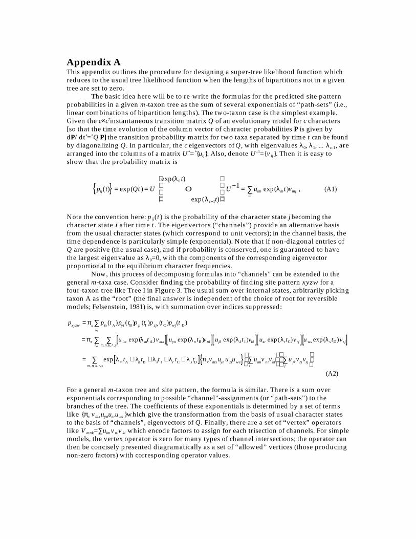
53

Appendix AThis appendix outlines the procedure for designing a super-tree likelihood function whichreduces to the usual tree likelihood function when the lengths of bipartitions not in a giventree are set to zero.

The basic idea here will be to re-write the formulas for the predicted site patternprobabilities in a given m-taxon tree as the sum of several exponentials of “path-sets” (i.e.,linear combinations of bipartition lengths). The two-taxon case is the simplest example.Given the c×c instantaneous transition matrix Q of an evolutionary model for c characters[so that the time evolution of the column vector of character probabilities P is given bydP/dt = Q P] the transition probability matrix for two taxa separated by time t can be foundby diagonalizing Q. In particular, the c eigenvectors of Q, with eigenvalues λ0, λ1, ... λc–1, arearranged into the columns of a matrix U = {uij}. Also, denote U–1={v ij}. Then it is easy toshow that the probability matrix is

pij(t){ } = exp(Qt) = U exp(λ0 t)

O

exp(λc−1t)

U−1 = uim exp(λmt)vmj

m∑ , (A1)

Note the convention here: p ij(t) is the probability of the character state j becoming thecharacter state i after time t. The eigenvectors (“channels”) provide an alternative basisfrom the usual character states (which correspond to unit vectors); in the channel basis, thetime dependence is particularly simple (exponential). Note that if non-diagonal entries ofQ are positive (the usual case), and if probability is conserved, one is guaranteed to havethe largest eigenvalue as λ0=0, with the components of the corresponding eigenvectorproportional to the equilibrium character frequencies.

Now, this process of decomposing formulas into “channels” can be extended to thegeneral m-taxa case. Consider finding the probability of finding site pattern xyzw for afour-taxon tree like Tree I in Figure 3. The usual sum over internal states, arbitrarily pickingtaxon A as the “root” (the final answer is independent of the choice of root for reversiblemodels; Felsenstein, 1981) is, with summation over indices suppressed:

pxyzw = πx pix(tA)pyi (tB )p ji (tI )p zjx (tC )pwj(t D)i, j∑

= πx u im exp(λmtA)vmx[ ] uyn exp(λntB )vni[ ] ujk exp(λ kt I )vki[ ] uzr exp(λrtC)vrj[ ] uws exp(λ stD)vsj[ ]m,n ,k ,r ,s

∑i , j∑

= exp λmtA + λntB + λ kt I + λr tC + λ stD[ ] π xvmxuyn u zruws{ } uimv nivkii∑

u jkvrj vsjj

∑

m ,n, k, r,s

∑

(A2)

For a general m-taxon tree and site pattern, the formula is similar. There is a sum overexponentials corresponding to possible “channel”-assignments (or “path-sets”) to thebranches of the tree. The coefficients of these exponentials is determined by a set of termslike {πx vmxuynuzruws }which give the transformation from the basis of usual character statesto the basis of “channels”, eigenvectors of Q. Finally, there are a set of “vertex” operatorslike Vmnk=∑uimvniv ki which encode factors to assign for each trisection of channels. For simplemodels, the vertex operator is zero for many types of channel intersections; the operator canthen be concisely presented diagramatically as a set of “allowed” vertices (those producingnon-zero factors) with corresponding operator values.

54

ee

e

ec

c

Figure A1. The vertex operator, in diagrammatic representation, for the simplest binary model. If the followingchannel intersections occur in the tree, a factor of 1 is given to the path-set; other intersections give factors of zero(i.e., are disallowed).

For the simplest binary model,

U =

12

1 11 −1

; (A3)

U–1 = 2 U; and the vertex operator is diagrammatically presented in Figure A1. There aretwo channels, the “equilibrium” (λe = 0) and “changing” (λc = –2) channels. Based on thesediagrammatic rules, it is easy to see that the only path-sets that will be included in aformula for a given site pattern are those which have c-channels threading through thetree in connected, non-intersecting lines; see the examples in Figure A2. For a given sitepattern the coefficient of the exponential is determined by assigning a factor 1/2 to eachtaxon starting in an e-channel, and a factor ±1/2 (sign depending on the taxon’s character forthat site pattern) for each taxon starting in a c-channel. The factors are multiplied to yielda coefficient ±1/2m. With these rules for finding the formulas for the site patternfrequencies, the log-likelihood function for a given tree is l = ∑ nilogp i, summed over all sitepatterns.

How then can one define a super-tree likelihood function? For an m-taxon tree, thepredicted site pattern probabilities take the form of a sum of several exponentials of sums ofthe bipartition lengths t. For the simplest binary model above, there are 2m–1 suchexponential terms, each corresponding to an allowed path-set; and each path-set term isuniquely determined by which pair (or quartet, hextet, etc.) of external branches is givenchannel label c. For different trees, there will be the same path-sets contributing to a givensite pattern probability; only the internal bipartition lengths going into the exponent ofeach path-set term will be different. To produce a formula for a super-tree site-patternprobability, one includes in the exponent of each path-set term any bipartition length thatmight show up for any tree. By construction, then the site-pattern probability reduces to theusual formula for a given tree when bipartitions not in that tree are set to zero. This is theprocedure used to find eq. (13) for the four-taxon tree in Section 2.4.

A similar, well-defined procedure can be defined for finding the super-tree sitepattern probabilities for a Kimura 3-state model, where the instantaneous transitionmatrix is:

Q = 

−1− κ 1 −κ 2 1 κ 1 κ2

1 −1− κ 1 −κ 2 κ 2 κ 1

κ 1 κ 2 −1− κ1 −κ 2 1κ 2 κ 1 1 −1− κ1 − κ 2

(A4)

55

Figure A2. Two sample path-sets for a 10-taxon tree. For each path-set – a labelling of each branch with a channel(light lines are the “e” channel; dark lines are the “c” channel)  –  there is an exponential term in the site patternprobability, with the exponent proportional to the sum of the lengths of all c-branches.

The matrix of eigenvectors is then:

U =14

+1 +1 +1 +1+1 −1 +1 −1+1 +1 −1 −1+1 −1 −1 +1

(A5)

and U–1 = 4 U . The eigenvalues of the channels are λe = 0; λc1 = –2 – 2κ2; λc2 = –2κ1 – 2κ2; andλc3 = –2 – 2κ1. The diagrammatic vertex rules are given in Figure A3. Again, each sitepattern probability is a linear combination of path-set exponentials. It can be shown thatfor any given tree, each path-set can be uniquely indexed based on the channel-labeling ofthe external branches only. Thus the site pattern probability for the super-tree can again bedetermined by including in the exponents of each path-set term all bipartition lengths thatmight show up for any tree.

The above construction of the super-tree fails for more general models. For example,in the binary model with unequal frequencies, the instantaneous rate matrix is:

Q =

−π 1 +π0

+π 1 −π0

, (A6)

and the matrix of eigenvectors, and its inverse can be written as:

U =

π0 +1/ 2π1 −1/ 2

;

U =

1 +2π 1

1 −2π0

;

with eigenvalues λe = 0 and λc = –2. The diagrammatic vertex rules are those given in FigureA4. However, here the path-set cannot be indexed solely based on the channel-labelling ofthe external branches; see Figure A5. Thus, it is somewhat arbitrary to decide whichpathset in a given tree corresponds to a given pathset in a different tree. The procedure fordefining the super-tree site pattern probability is still possible, but not unique.

56

ec3

c3

ec1

c1

ec2

c2

ee

e

c1c2

c3

Figure A3. The vertex operator, in diagrammatic representation, for the Kimura 3-state model. If the followingchannel intersections occur in the tree, a factor of 1 is given to the path-set; other intersections give factors of zero(i.e., are disallowed).

ee

e

ec

c

cc

c

Figure A4. The vertex operator, in diagrammatic representation, for the binary model with unequal frequencies. Thefollowing channel intersections give non-zero values. In particular, the third vertex gives a factor proportional toπ0 – π1, and is therefore zero only in the equal frequency case (see Figure A1).

57

c

c

c

c

e

c

c

c

c

c

Figure A5. Two path-sets which contribute separate exponential terms in the formulas site pattern probabilities forthe binary model with unequal frequencies, but which have the same channel labelling of external branches.

For models like HKY85 for DNA sequences the Dayhoff matrix for amino-acidsequences, the result is the same: the super-tree site pattern probabilities can be defined, butnot necessarily uniquely.16 Indeed, the super-tree probabilities given above for the simplestbinary model and the Kimura three-state model are not unique, either. Those simpleprocedures can easily be modified by extra terms which will not perturb their limits forindividual tree hypotheses. However, the procedures above are useful for obtaining well-defined, especially simple formulas, with intuitive properties like the additivity relationfor pair-wise distances given in Section 2.4 for the simplest binary model. Defining suchprocedures for more general models, possibly based on geometrical pictures like Figure 3, iscurrently under investigation.

Appendix BThe mean and variance of the normal distribution of statistics like (lmax– lI) described inSection 3.1 are approximated as follows. For a finite number of sites n, the full cm–1 sitepatterns are not expected to be seen in the data set; indeed, many real data sets aredominated by sites which are the same in all or most taxa [“sparseness” of the data; see,e.g., (Goldman, 1993), (Yang et al., 1995)]. A first guess might be to assume that each sitepattern with non-zero frequency constitutes one degree of freedom; the contributions of eachdegree of freedom to the mean and variance of (lmax– lI) are 1/2 and 1/2, respectively. Theoverall mean and variance would be predicted to be (npatt–nparam)/2 and npatt/2, respectively.

In actuality, site patterns which do not appear in the given data set still make acontribution to the mean and variance of (lmax– lI). Given the expected probability p i of a

given site pattern, the contribution of that site pattern to the mean and variance to (lmax– lI),under Poisson statistics, are explicitly

l max(i) − lI

( i) =npi( )q

e − npi

q!

q =0

∞

∑ q log q( ) − q( ) − q log np i( ) − np i( )[ ]

lmax(i) − lI(i)( )2

=npi( )q

e − npi

q!

q =0

∞

∑ q log q( ) − q( ) − q log np i( ) − np i( )[ ]2

Var lmax( i ) − l I

( i )[ ] = l max( i) − l I

( i)( )2− lmax

(i ) − lI(i)

(B1)

The functions for the mean and variance are plotted in Figure B1; it is seen that bothfunctions approach 1/2 quickly for pi > 1, but are nevertheless non-vanishing pi<0. For a real

16 It is clear, in fact, that the super-tree site pattern probabilities can be defined for any model, reversible or not.Basically, in describing the site pattern probabilities, there are (N – 1) × 2B possible pathset coefficients, where B is thenumber of possible bipartitions times the number of characters, and N is the number of site patterns (cm). One canalways choose the coefficients to satisfy the smaller number of (N – 1) × 2[c (2m – 5)] constraints obtained in forcing thesuper-tree likelihood function to reduce to the usual tree likelihood functions when bipartitions not in a given treeare set to zero.

58

data set, one thus needs estimates of pi for all site patterns with predicted frequenciesgreater than, say, 1/10; the accuracy of the estimates for pi > 1 is not terribly critical. Thisestimation can easily be done for a given data set by optimising branch lengths andevolutionary parameters for any tree close to the expected maximum likelihood tree. Theresulting parameters are then used in, e.g., PAML's evolver program, to simulate a data setwith, say, 10 times as many sites as the data set under consideration. Then the formula (B1)is applied to non-vanishing site pattern frequencies of the simulated data set, and summedto find the overall predicted mean and variance of the (lmax– lI) distribution. If a number

nparam of parameters are fitted to obtain lI, the predicted mean should be decreased byapproximately nparam/2. In this report, for DNA and amino acid data, a simulated data set100 times and 10,000 times, respectively, the length of the real data set is constructed.

Of course, an alternative way to find the predicted mean and variance would be toactually do, say 100 simulations of data sets of the same length as the real data set, and tofind (lmax– lI) for each replicate. See Yang (1994) for examples. This latter procedure isgenerally much more time-consuming, since the likelihood parameters need to be optimisedfor each simulated replicate. Estimates from both procedures agree (see Figure 11).

0 1 2 3 4 5 6 7 8 9 100.0

0.1

0.2

0.3

0.4

0.5

0.6

0.7

Expectation value of Poisson distribution

Figure B1. Mean (dark thick line) and variance (grey thin line) of l– l max for Poisson distributions with differentexpectation values.