theoretical and numerical study of tikhonov's regularization and morozov's discrepancy...
TRANSCRIPT

Georgia State UniversityScholarWorks @ Georgia State University
Mathematics Theses Department of Mathematics and Statistics
12-2009
Theoretical and Numerical Study of Tikhonov'sRegularization and Morozov's DiscrepancyPrincipleMaryGeorge L. WhitneyGeorgia State University
Follow this and additional works at: https://scholarworks.gsu.edu/math_theses
Part of the Mathematics Commons
This Thesis is brought to you for free and open access by the Department of Mathematics and Statistics at ScholarWorks @ Georgia State University. Ithas been accepted for inclusion in Mathematics Theses by an authorized administrator of ScholarWorks @ Georgia State University. For moreinformation, please contact [email protected].
Recommended CitationWhitney, MaryGeorge L., "Theoretical and Numerical Study of Tikhonov's Regularization and Morozov's Discrepancy Principle."Thesis, Georgia State University, 2009.https://scholarworks.gsu.edu/math_theses/77

THEORETICAL AND NUMERICAL STUDY OF TIKHONOV’S
REGULARIZATION AND MOROZOV’S DISCREPANCY PRINCIPLE
by
MARYGEORGE L. WHITNEY
Under the Direction of Dr. Alexandra Smirnova
ABSTRACT
A concept of a well-posed problem was initially introduced by J. Hadamard in 1923,
who expressed the idea that every mathematical model should have a unique solution,
stable with respect to noise in the input data. If at least one of those properties is
violated, the problem is ill-posed (and unstable). There are numerous examples of ill-
posed problems in computational mathematics and applications. Classical numerical
algorithms, when used for an ill-posed model, turn out to be divergent. Hence one has to
develop special regularization techniques, which take advantage of an a priori information
(normally available), in order to solve an ill-posed problem in a stable fashion. In this
thesis, theoretical and numerical investigation of Tikhonov’s (variational) regularization
is presented. The regularization parameter is computed by the discrepancy principle of
Morozov, and a first-kind integral equation is used for numerical simulations.
INDEX WORDS: Tikhonov regularization, Morozov discrepancy principle, Ill-posed problems, Newton’s method, Georgia State University

THEORETICAL AND NUMERICAL STUDY OF TIKHONOV’S
REGULARIZATION AND MOROZOV’S DISCREPANCY PRINCIPLE
by
MARYGEORGE L. WHITNEY
A Thesis Submitted in Partial Fulfillment of the Requirements for the Degree of
Master of Science
in the College of Arts and Sciences
Georgia State University
2009

Copyright byMaryGeorge Llewellyn Whitney
2009

THEORETICAL AND NUMERICAL STUDY OF TIKHONOV’S REGULAIZATION
AND MOROZOV’S DISCREPANCY PRINCIPLE
by
MARYGEORGE L. WHITNEY
Chair:
Committee:
Dr. Alexandra Smirnova
Dr. Michael Stewart
Dr. Vladimir Bondarenko
Electronic Version Approved:
Office of Graduate Studies
College of Arts and Sciences
Georgia State University
December 2009

iv
This thesis is dedicated to Floyd Clifford Whitney III,
Dr. Alexandra Smirnova,
and Dr. Rachael Belinsky.

v
ACKNOWLEDGEMENTS
I would like to thank my advisor, Dr. Alexandra Smirnova, for all of her guidance
and support, and her never ending patience. I have learned so much. Thank you for the
extraordinary example.
I would also like to thank Dr. Michael Stewart and Dr. Vladimir Bondarenko whose
willingness to aid in my education are just two examples of the quality professors we have
here at Georgia State University.
I would like to also thank my husband, without whom I would have never gone back
to school. Thank you for making a dream come true. To my children, their support and
encouragement inspired me to want to be the best I could be. Finally, to Dr. Rachael
Belinsky, who has been a friend, mentor, and a beacon of strength, thank you. To my
other family and friends, thank you for your support, encouragement, and patience.

vi
TABLE OF CONTENTS
ACKNOWLEDGEMENTS . . . . . . . . . . . . . . . . . . . . . . . . . . . . v
LIST OF FIGURES . . . . . . . . . . . . . . . . . . . . . . . . . . . . . . . . . viii
LIST OF TABLES . . . . . . . . . . . . . . . . . . . . . . . . . . . . . . . . . . ix
Chapter 1 INTRODUCTION . . . . . . . . . . . . . . . . . . . . . . . . . 1
Chapter 2 UNSTABLE MODELS . . . . . . . . . . . . . . . . . . . . . . 3
2.1 Examples of Ill-posed Problems . . . . . . . . . . . . . . . . . . . . . . . 3
2.2 Numerical Aspects . . . . . . . . . . . . . . . . . . . . . . . . . . . . . . 9
2.3 A General Regularization Strategy . . . . . . . . . . . . . . . . . . . . . 10
Chapter 3 THE REGULARIZATION THEORY . . . . . . . . . . . . . 15
3.1 The Tikhonov (Variational) Regularization . . . . . . . . . . . . . . . . . 15
3.2 The Discrepancy Principle of Morozov . . . . . . . . . . . . . . . . . . . 20
Chapter 4 NUMERICAL SIMULATIONS . . . . . . . . . . . . . . . . . 24
4.1 Statement of the Problem . . . . . . . . . . . . . . . . . . . . . . . . . . 24
4.2 Sources of Noise . . . . . . . . . . . . . . . . . . . . . . . . . . . . . . . . 28

vii
4.3 Simulation . . . . . . . . . . . . . . . . . . . . . . . . . . . . . . . . . . . 31
Chapter 5 DISCUSSION . . . . . . . . . . . . . . . . . . . . . . . . . . . . 34
5.1 Summary . . . . . . . . . . . . . . . . . . . . . . . . . . . . . . . . . . . 34
5.2 Advantages . . . . . . . . . . . . . . . . . . . . . . . . . . . . . . . . . . 35
5.3 Disadvantages . . . . . . . . . . . . . . . . . . . . . . . . . . . . . . . . . 37
REFERENCES . . . . . . . . . . . . . . . . . . . . . . . . . . . . . . . . . . . . 38
APPENDIX A . . . . . . . . . . . . . . . . . . . . . . . . . . . . . . . . . . . . 40
APPENDIX B . . . . . . . . . . . . . . . . . . . . . . . . . . . . . . . . . . . . 44
APPENDIX C . . . . . . . . . . . . . . . . . . . . . . . . . . . . . . . . . . . . 48
APPENDIX D . . . . . . . . . . . . . . . . . . . . . . . . . . . . . . . . . . . . 54
APPENDIX E . . . . . . . . . . . . . . . . . . . . . . . . . . . . . . . . . . . . 55

viii
LIST OF FIGURES
2.1 Ill-posed and Well-posed linear systems . . . . . . . . . . . . . . . . . . . 7
2.2 Exact and Approximate Solutions . . . . . . . . . . . . . . . . . . . . . . 11
2.3 Error Estimation for the Central Difference Formula . . . . . . . . . . . . 12
4.1 Exact and Approximate Solutions for σ = 0.0001 . . . . . . . . . . . . . 27
4.2 Exact and Approximate Solutions for σ = 0.05 . . . . . . . . . . . . . . . 29
4.3 Exact and Approximate Solutions for σ = 0.1 . . . . . . . . . . . . . . . 29
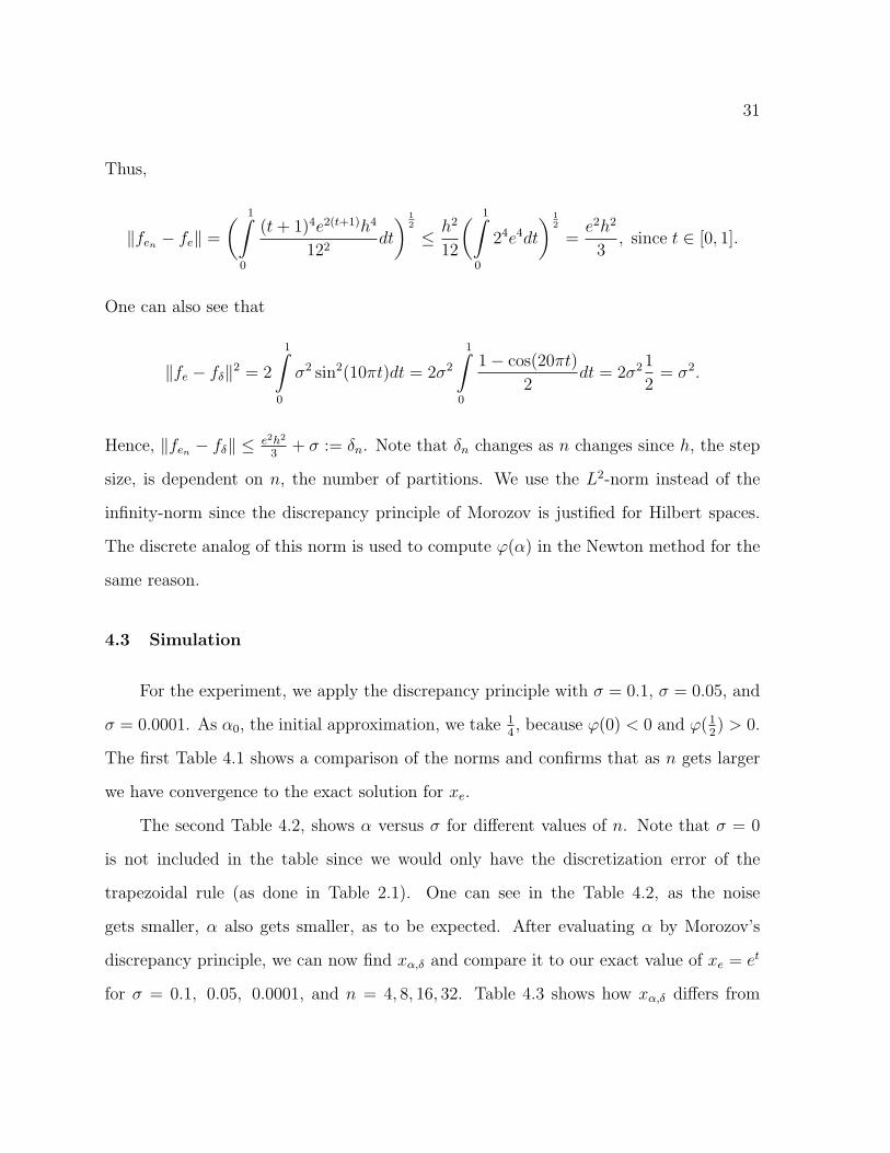
4.4 Exact and Approximate Solutions for n = 32 . . . . . . . . . . . . . . . . 32
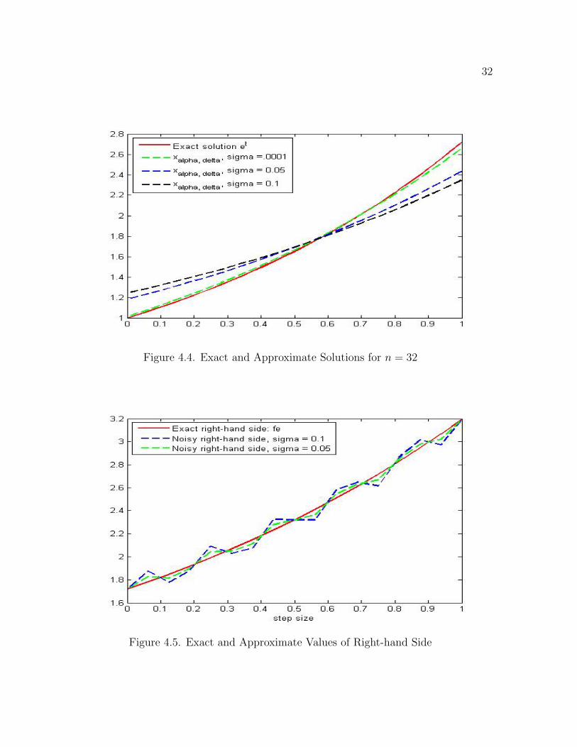
4.5 Exact and Approximate Values of Right-hand Side . . . . . . . . . . . . 32
5.1 Exact and Approximate Solutions . . . . . . . . . . . . . . . . . . . . . . 36
5.2 Exact and Approximate Solution for σ = 0.05 . . . . . . . . . . . . . . . 36

ix
LIST OF TABLES
2.1 Comparative Results . . . . . . . . . . . . . . . . . . . . . . . . . . . . . 10
4.1 Comparison of Errors . . . . . . . . . . . . . . . . . . . . . . . . . . . . . 25
4.2 Values of α by Discrepancy Principle . . . . . . . . . . . . . . . . . . . . 25
4.3 Comparative Results for σ = 0.0001 . . . . . . . . . . . . . . . . . . . . . 26
4.4 Comparative Results for σ = 0.05 . . . . . . . . . . . . . . . . . . . . . . 28
4.5 Comparative Results for σ = 0.1 . . . . . . . . . . . . . . . . . . . . . . . 28
5.1 Results for the ’Naive’ Discretization . . . . . . . . . . . . . . . . . . . . 35
5.2 Comparative Results for σ = 0.05 . . . . . . . . . . . . . . . . . . . . . . 35

1
Chapter 1
INTRODUCTION
The definition of a well-posed problem was originally introduced by J. Hadamard
[6] in 1923 in order to figure out what types of boundary conditions are to be used for
various types of differential equations. Hadamard’s concept reflected the idea that any
mathematical model of a physical problem must have the properties of uniqueness, exis-
tence, and stability of the solution. If at least one of these properties is not satisfied, the
problem is ill-posed. Among classical ill-posed problems are stable numerical differenti-
ation of noisy data, stable inversion of ill-conditioned matrices, parameter identification
in partial differential equations, stable solution of first-kind integral equations, and many
other examples.
Let X and Y be normed spaces and the problem
Kx = f, K : X → Y (1.1)
be ill-posed. Suppose the right-hand side f is given by its δ-approximation, fδ, such that
‖f − fδ‖ ≤ δ. It would be natural to seek an approximate solution to (1.1) in the set
Qδ := {x ∈ X : ‖Kx − fδ‖ ≤ δ}. However, in the ill-posed case an arbitrary element
xδ ∈ Qδ can not be used as an approximate solution to (1.1). Since xδ does not depend
continuously on fδ, the fact that ‖Kx − fδ‖ ≤ δ does not guarantee that xδ is close to

2
the solution we are looking for.
Thus, if problem (1.1) is ill-posed, one has to use a priori information (normally
available) in order to solve the problem in a stable manner, i.e., to construct a regular-
ized solution to (1.1). Such a priori information as smoothness of the solution generates
the technique, which is called Tikhonov (variational) regularization [15] [14]. This
regularization allows one to obtain stable approximate solutions to ill-posed problems
by means of a stabilizing functional. Initially proposed by A. Tikhonov, the variational
methods have been further developed in [13], [5], [3], [8], [16].
One can also find approximate solutions to (1.1) by iterations (see [1], [17], [18],
[7]), taking xn = F (fδ, xn−1, ..., xn−k), where k ≤ n. For these solutions to be stable
under small changes in the initial data, the iteration number n = n(δ) yielding xn must
be compatible with the size of the error in the initial data.
Another important approach to the theory of ill-posed problems is based on the
singular value decomposition (SVD) of a compact operator in a Hilbert space. Using
SVD, one obtains an admissible regularization strategy by proper filtering of the singular
system.
This thesis is organized as follows:
• Chapter 2. Examples of ill-posed problems and the regularization overview.
• Chapter 3. The Tikhonov regularization theory.
• Chapter 4. Numerical simulations.
• Chapter 5. Conclusions

3
Chapter 2
UNSTABLE MODELS
2.1 Examples of Ill-posed Problems
In this section, we give some fundamental results and definitions related to the theory
of ill-posed problems. We also present and discuss some important examples of unstable
mathematical models.
We start with the definition of a norm. The norm will be used to measure distance
between two functions. In what follows, it will be the distance between exact and noisy
data, and between exact and approximate solutions.
Definition 2.1.1. [2] Let X be a vector space over the field R (C). X is normed, if there
is a function || · ||: X→ R (C), which we call a norm, satisfying all of the following:
1. ||f || ≥ 0, and ||f || = 0 if and only if f = 0 (positive definiteness),
2. ||αf || = |α| ||f || for any real (or complex) scalar α (homogeneity),
3. ||f + g|| ≤ ||f ||+ ||g|| (the triangle inequality).
Definition 2.1.2. [9] Let X and Y be normed spaces, and K : X → Y (not necessarily
onto). The problem of finding a solution x ∈ X from the data f ∈ Y , Kx = f , is called
well-posed, or properly posed if the following are all true:

4
1. Existence: For every f ∈ Y there is (at least one) x ∈ X such that Kx = f (K is
onto).
2. Uniqueness: For every f ∈ Y there is at most one x ∈ X with Kx = f (K is
one-to-one).
3. Stability: The solution x depends continuously on f ∈ Y , i.e., for every {xn} ⊂ X
with Kxn → Kx, (n→∞), it follows that xn → x, (n→∞).
If at least one condition is violated then the problem is ill-posed or unstable.
The first example is one in partial differential equations involving an initial value
problem for the Laplace equation. In fact, this is Cauchy’s problem for the Laplace
equation, a classic example that was done by Hadamard [6].
Example 2.1.3. The noisy data is denoted by fδ and gδ and the exact data is denoted
by fe and ge. Consider the Laplace equation:
∆u(x, t) =∂2u
∂x2+∂2u
∂t2= 0, x ∈ R, t ∈ [0,∞) ,
with the initial conditions
u(x, 0) = f(x) and∂u
∂t(x, 0) = g(x), x ∈ R.
Suppose
fe(x) = ge(x) = 0 and fδ(x) = 0, gδ(x) = δ sin(xδ
), δ > 0
We now introduce the norm in the data space as ‖(f, g)‖ := supx∈R{|f | + |g|}, and the
norm in the solution space as ‖u‖ := supx∈R |u(x, t)|. One has
‖(fδ − fe, gδ − ge)‖ = supx∈R{|fδ − fe|+ |gδ − ge|} = sup
x∈R{|fδ|+ |gδ|}

5
= supx∈R
{|0|+
∣∣∣δ sin(xδ
)∣∣∣} = supx∈R
{∣∣∣δ sin(xδ
)∣∣∣} = δ.
For the noisy data, one can show that the corresponding solution
uδ(x, t) = δ2 sin(xδ
)sinh
( tδ
)x ∈ R, t ≥ 0.
Indeed, the partial derivatives are as follows:
(uδ)x = δ cos(xδ
)sinh
( tδ
), and (uδ)t = δ sin
(xδ
)cosh
( tδ
).
The second partial derivatives are
(uδ)xx = − sin(xδ
)sinh
( tδ
), and (uδ)tt = sin
(xδ
)sinh
( tδ
).
These derivatives will then give us (uδ)xx + (uδ)tt = ∆uδ(x, t) = 0. For the exact data,
ue(x, t) = 0, x ∈ R, t ≥ 0. Therefore
‖(uδ − ue)‖ = supx∈R
∣∣∣uδ(x, t)− ue(x, t)∣∣∣ = supx∈R
∣∣∣δ2 sin(xδ
)sinh
( tδ
)∣∣∣ = δ2∣∣∣sinh
( tδ
)∣∣∣= δ2 e
tδ − e−tδ
2
Let δ = 1n, then for any t > 0, limn→∞
ent−e−nt2n2 = (∞∞), since by repeated use of L’Hopital’s
rule we end up with t2
4limn→∞ e
nt−e−nt =∞. So, ‖(fδ−fe, gδ−ge)‖ = δ → 0, as δ → 0,
while ‖uδ − ue‖ does not approach 0 as δ goes to 0. This means the problem is ill-posed.
In the following example we look at a differentiation problem to show how the slight
change in the data can cause a considerable change in the solution. The noisy data is
denoted by fδ. The exact data is denoted by fe.

6
Example 2.1.4. Let fe(x) = 0 and fδ(x) = δ sin( xδ2
). Using the infinity norm we get
‖fe − fδ‖∞ = supx∈R
∣∣∣0− δ sin( xδ2
)∣∣∣ = supx∈R|δ|∣∣∣sin( x
δ2
)∣∣∣ = δ.
Now if we take the derivatives of f(x) we get f ′e(x) = 0 and f ′δ(x) = 1δ
cos( xδ2
). Using the
infinity norm in the solution space we then get ‖f ′δ − f ′e‖∞ = supx∈R |1δ cos( xδ2
)− 0| = 1δ,
and as δ goes to 0 the supremum goes to infinity. This means that the differentiation
problem is unstable or ill-posed.
In the next example we use a matrix norm and a vector norm to analyze an ill-
conditioned liner system Ax = f . Assume that A is a nonsingular matrix, fδ is a
perturbed (or noisy) right-hand side, and fe is the exact right-hand side.
Example 2.1.5. Solving for x we get xe − xδ = A−1(fe − fδ), and solving for fe we get
‖fe‖ = ‖Axe‖ ≤ ‖A‖ ‖xe‖ . . .⇒ 1‖xe‖ ≤
‖A‖‖fe‖ . We will use these facts while solving for the
relative error as follows:
‖xe − xδ‖‖xe‖
≤ ‖A−1‖ ‖fe − fδ‖‖xe‖
= ‖A−1‖ ‖fe − fδ‖‖fe‖
‖A‖
≤ ‖A‖ ‖A−1‖︸ ︷︷ ︸cond(A)
‖fe − fδ‖‖fe‖
.
One can see from above that a large condition number can result in a considerable
change in the solution even if the relative change in the right-hand side is small (unstable
problem). In fact, cond(A) measures how close A is to a singular matrix. The following
theorem helps to explain.
Theorem 2.1.6. [4] Let A ∈ Rn×n be nonsingular. Then for any singular matrix B ∈
Rn×n, 1
cond(A)≤ ‖A−B‖
‖A‖ .

7
Figure 2.1. Ill-posed and Well-posed linear systems
So, as A gets close to singular, cond(A) approaches infinity. In the two dimensional
case represented by a two-by-two system,
[~a1 ~a2
]x1
x2
= ~b
⇔ ~a1x1 + ~a2x2 = ~b⇔ ~a1x1 = ~b− ~a2x2
i.e., the solution is equivalent to finding the intersection of the one dimensional subspace
{x~a1 : x ∈ R} with the affine subspace {~b− ~a2x : x ∈ R}. Such intersections are shown in
Figure 2.1. If the subspaces are nearly parallel to the solution then the condition number
is large since the matrix is almost singular, and a slight perturbation in the system may
result in a considerable change of the solution. On the other hand, if the subspaces are
almost perpendicular to the solution, a small perturbation or slight shift means you will
still get a good solution.
Next we go to linear equations with compact operators Kx = f using the following

8
definition:
Definition 2.1.7. K is a compact operator if it is a linear operator from a Banach space
X to a Banach space Y such that the image under K for any bounded subset of X is a
relatively compact set (its closure is compact).
Theorem 2.1.8. [9] Linear equations Kx = f with compact operators K : X → Y ,
where X and Y are normed spaces and dimX =∞ are always ill-posed.
Proof :
To show that Kx = f is ill-posed, we will prove that K−1 is unbounded. Assume
the converse: K−1 exists and is bounded, then K−1K = I should be compact since a
superposition of a bounded and compact operators is a compact operator. Contradiction,
since a unit ball in infinite dimensional space is not a compact set.�
The following is an example of an ill-posed equation with a compact operator:
Kx :=
b∫a
k(t, s)x(s)ds = f(t), K : X → Y, t ∈ (c, d).
This comes from the following theorem:
Theorem 2.1.9. [9]
(a) Let k(t, s) ∈ L2(
(c, d)× (a, b))
. The operator K : L2(a, b)→ L2(c, d), defined by
Kx :=
b∫a
k(t, s)x(s)ds, t ∈ (c, d), x ∈ L2(a, b),
is compact from L2(a, b) into L2(c, d).
(b) Let k(t, s) be continuous on [c, d] × [a, b]. Then K defined by the integral above is
also compact as an operator from C[a, b] into C[c, d].

9
2.2 Numerical Aspects
The following example was initially done by Kirsch, [9], but is done here in a different
way. While the conclusions are the same, the outcomes and methods used are different.
In both cases, the results lead to the conclusion that the problem is ill-posed, but the
numerical outcomes and the way in which they were obtained are different. The Matlab
code used and the results can be seen in Appendix A and B respectively.
Example 2.2.1. [9] Consider the integral equation
Kx :=
1∫0
etsx(s)ds = f(t), K : C[0, 1]→ C[0, 1],
where 0 ≤ t ≤ 1. Let f(t) = et+1−1t+1
. The unique solution is x(t) = et. We are to
approximate the integral using the trapezoidal rule as follows:
1∫0
etsx(s)ds ≈ h
[1
2x(0) +
1
2etx(1) +
n−1∑j=1
ejhtx(jh)
]≈ f(t),
where h = 1n
and t = ih. The vector [x0 x1 . . . xn]T represents the numerical solution
given the right-hand side [f0 f1 . . . fn]T . For the experiment we take n = 4, 8, 16, 32 as
the number of partitions and t = 0, 0.25, 0.5, 1 to compare the solutions corresponding to
different values of n. Using a table for n vs. t we are to compute x(ti) − xi in Matlab.
See Appendix A for Matlab code and Appendix B for the results for n = 16, and n = 32.
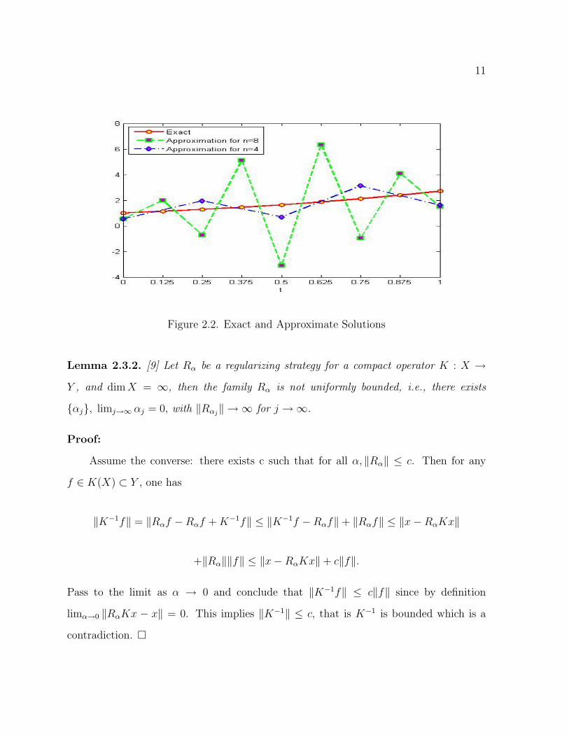
The Figure 2.2 illustrates the numerical results for n = 4 and n = 8 as compared to the
exact solution. Please note that in the Matlab code, the statement x = K\f means that
x is determined by the division of K into f , which is roughly the same as inv(K) ∗ f
except that it is calculated by Gaussian elimination and forward/backward substitution,
with no explicit computation of the inverse.

10
Table 2.1. Comparative Results
x(ti)− xit n = 4 n = 8 n = 16 n = 32 x(ti) = exp(ti)0 0.56 0.53 -3.20 -31.14 1.00
0.25 1.95 -0.74 45.30 13.40 1.280.50 0.69 -3.11 24.17 -12.32 1.650.75 3.13 -0.95 66.94 33.04 2.121.0 1.63 1.49 -0.72 -9.83 2.72
The table given in Kirsch [9] was done by calculating the inv(K) and then multiplying by
f instead of using the Gaussian elimination. This is known to be numerically unstable.
Since Matlab does not calculate the inv(K) our solutions are more accurate than those
given by Kirsch. They agree with those computed by Kirsch for n = 4 only. Still, as
n gets larger the approximation gets worse, to the point that matrix K becomes nearly
singular at n = 16, causing a very bad approximation that gets even worse at n = 32.
See Table 2.1 and Appendix B for results of the exercise.
Since K−1 is unbounded for the original infinite-dimensional problem, the matrix
becomes closer to singular as the number of partitions increases. The finer the discretiza-
tion, the worse the approximation, i.e., the problem is ill-posed.
2.3 A General Regularization Strategy
To present the general concept of a regularization strategy, we begin with the defi-
nition:
Definition 2.3.1. [9] A regularizing strategy is a family of linear and bounded operators
Rα : Y → X, α > 0 such that limα→0 ‖RαKx− x‖ = 0 for all x ∈ X, i.e., the operators
RαK converge pointwise to the identity.
11
Figure 2.2. Exact and Approximate Solutions
Lemma 2.3.2. [9] Let Rα be a regularizing strategy for a compact operator K : X →
Y , and dimX = ∞, then the family Rα is not uniformly bounded, i.e., there exists
{αj}, limj→∞ αj = 0, with ‖Rαj‖ → ∞ for j →∞.
Proof:
Assume the converse: there exists c such that for all α, ‖Rα‖ ≤ c. Then for any
f ∈ K(X) ⊂ Y , one has
‖K−1f‖ = ‖Rαf −Rαf +K−1f‖ ≤ ‖K−1f −Rαf‖+ ‖Rαf‖ ≤ ‖x−RαKx‖
+‖Rα‖‖f‖ ≤ ‖x−RαKx‖+ c‖f‖.
Pass to the limit as α → 0 and conclude that ‖K−1f‖ ≤ c‖f‖ since by definition
limα→0 ‖RαKx − x‖ = 0. This implies ‖K−1‖ ≤ c, that is K−1 is bounded which is a
contradiction. �

12
Figure 2.3. Error Estimation for the Central Difference Formula
Let xα,δ := Rαfδ. Then E(α) := ‖xα,δ − xe‖ estimates how good the approximation
is for fδ. Suppose ‖fδ − fe‖ ≤ δ. Then
E(α) = ‖xα,δ − xe‖ = ‖Rαfδ −Rαfe +Rαfe − xe‖ ≤ ‖Rαfδ −Rαfe‖+ ‖Rαfe − xe‖
≤ ‖Rα(fδ − fe)‖+ ‖Rαfe − xe‖ ≤ ‖Rα‖‖fδ − fe‖+ ‖Rαfe − xe‖
≤ ‖Rα‖δ + ‖RαKxe − xe‖. (2.3.2.1)
Note as α approaches 0, ‖Rα‖δ approaches infinity and ‖RαKxe − xe‖ approaches
0. This is the fundamental estimate for a regularization strategy.
We illustrate this estimate by constructing a regularization strategy for the numerical
differentiation problem using the central difference formula and the step size h as a
regularization parameter.

13
Example 2.3.3. Let the derivative be approximated at t0 ∈ (a, b), and h be the step size.
Suppose ‖fδ − fe‖ = supt∈[t0−h,t0+h] ‖fδ(t)− fe(t)‖ = δ and Rhfδ(t0) = fδ(t0+h)−fδ(t0−h)2h
.
By using the central difference formula one gets
E(h) :=∣∣f ′e(t0)−Rhfδ(t0)
∣∣ =
∣∣∣∣f ′e(t0)− fδ(t0 + h)− fδ(t0 − h)
2h
∣∣∣∣=
∣∣∣∣f ′e(t0)− fδ(t0 + h)− fδ(t0 − h)
2h+fe(t0 + h)− fe(t0 + h)− fe(t0 − h) + fe(t0 − h)
2h
∣∣∣∣≤∣∣∣∣f ′e(t0)− fe(t0 + h)− fe(t0 − h)
2h
∣∣∣∣+ |fδ(t0 + h)− fe(t0 + h)|2h
+|fδ(t0 − h)− fe(t0 − h)|
2h.
Let us estimate the first term that measures the accuracy of the central difference formula.
One has
fe(t0 + h) = fe(t0) + f ′e(t0)h+f ′′e (t0)h
2
2+f ′′′e (ξ)h3
3!, ξ ∈ [t0, t0 + h],
and fe(t0 − h) = fe(t0)− f ′e(t0)h+f ′′e (t0)h
2
2− f ′′′e (µ)h3
3!, µ ∈ [t0 − h, t0].
By subtracting the two and using the mean value theorem one derives
fe(t0 + h)− fe(t0 − h) = 2f ′e(t0)h+f ′′′e (η)h3
3, η ∈ [t0 − h, t0 + h].
Solving for the f ′′′e (η)h2
6we get the following:
f ′′′e (η)h2
6=fe(t0 + h)− fe(t0 − h)
2h− f ′e(t0).
Thus, ∣∣∣∣f ′e(t0)− fe(t0 + h)− fe(t0 − h)
2h
∣∣∣∣ ≤ M3h2
6,
if supt∈[t0−h,t0+h] |f ′′′(t)| = M3. The second and third terms in the estimate for E(h) are

14
bounded by δ2h
. Hence
E(h) ≤ M3h2
6+δ
h, ‖Rhfe − f ′e‖ ≤
M3h2
6→ 0 and ‖Rα(fδ − fe)‖ ≤
δ
h→∞.
Now if we take the derivative of E(h) = M3h2
6+ δ
hwith respect to h and equate it to zero,
we will get the optimal value of the regularization parameter
E ′(h) =M3h
3− δ
h2=M3h
3 − 3δ
3h2= 0.
Solving for h we then have M3h3−3δ = 0, finally getting hopt =
(3δM3
)1/3as can be seen in
Figure 2.3. Note that hopt, which plays the role of α in this example, is the point where
the minimum of E(h) is attained. Therefore E(hopt) =(
98M3δ
2)1/3
.

15
Chapter 3
THE REGULARIZATION THEORY
3.1 The Tikhonov (Variational) Regularization
We begin with some important definitions:
Definition 3.1.1. [9] Let X be a vector space over the field K = R or K = C. A
scalar product or inner product is a mapping
〈·, ·〉 : X ×X → K
with the following properties:
(i) 〈x+ y, z〉 = 〈x, z〉+ 〈y, z〉 for all x, y, z ∈ X,
(ii) 〈αx, y〉 = α 〈x, y〉 for all x, y ∈ X and α ∈ K,
(iii) 〈x, y〉 = 〈y, x〉 for all x, y ∈ X,
(iv) 〈x, x〉 ∈ R and 〈x, x〉 ≥ 0, for all x ∈ X,
(v) 〈x, x〉 > 0 if x 6= 0.
The following properties are easily derived from the definition:

16
(vi) 〈x, y + z〉 = 〈x, y〉+ 〈x, z〉 for all x, y, z ∈ X,
(vii) 〈x, αy〉 = α 〈x, y〉 for all x, y ∈ X and α ∈ K.
Definition 3.1.2. [9] A vector space X over K with inner product 〈·, ·〉 is called a
pre-Hilbert space over K.
Definition 3.1.3. [9] A normed space X over K is called complete or a Banach space
if every Cauchy sequence converges in X. A complete pre-Hilbert space is called a
Hilbert space.
Definition 3.1.4. [9] Let : K : X → Y be a linear bounded operator between Hilbert
spaces. Then there exists a unique linear bounded operator K∗ : Y → X with the
property 〈Kx, y〉 = 〈x,K∗y〉 for all x ∈ X, y ∈ Y . The operator K∗ : Y → X is called
the adjoint operator to K. For X = Y , the operator K is called self-adjoint if K∗ = K.
A common approach to overdetermined linear systems of the form Kx = f is to solve
them in the sense of least squares, i.e., to minimize ‖Kx− f‖ with respect to x ∈ X. If
X is infinite-dimensional and K is a compact operator, the above minimization problem
is also ill-posed by the following lemma.
Lemma 3.1.5. [9] Let X, Y be Hilbert spaces such that K : X → Y , is linear and
bounded. Then there exists x ∈ X such that x = arg minx∈X ‖Kx − f‖, where arg min
is the element that minimizes ‖Kx − f‖, if and only if x solves the normal equation
K∗Kx = K∗f . K∗ : Y → X.

17
Proof:
‖Kx− f‖2 − ‖Kx− f‖2 = 〈Kx− f,Kx− f〉 − ‖Kx− f‖2
= 〈K(x− x) +Kx− f,K(x− x) +Kx− f〉 − ‖Kx− f‖2
= ‖K(x− x)‖2 + 〈K(x− x), Kx− f〉+
+ 〈Kx− f,K(x− x)〉+ ‖Kx− f‖2 − ‖Kx− f‖2
= ‖K(x− x)‖2 + 〈K(x− x), Kx− f〉+ 〈Kx− f,K(x− x)〉
= ‖K(x− x)‖2 + 〈Kx− f,K(x− x)〉+ 〈Kx− f,K(x− x)〉
= ‖K(x− x)‖2 + 2<e 〈Kx− f,K(x− x)〉
= ‖K(x− x)‖2 + 2<e 〈K∗(Kx− f), x− x〉 .
1. If K∗Kx = K∗f , then 2<e 〈K∗(Kx− f), x− x〉 = 0 and
‖Kx− f‖2 − ‖Kx− f‖2 = ‖K(x− x)‖2 ≥ 0, that is x minimizes ‖Kx− f‖.
2. Now let x be a minimizer of ‖Kx− f‖. Substitute x = x+ tz, z ∈ X, t > 0, then
0 ≤ ‖K(x− x)‖2 + 2<e 〈Kx− f,K(x− x)〉
= ‖K(tz)‖2 + 2<e 〈Kx− f,K(tz)〉
= t2‖Kz‖2 + 2t<e 〈Kx− f,Kz〉 .
Divide by t and pass to the limit as t approaches 0 to get:
0 ≤ t‖Kz‖2 + 2<e 〈Kx− f,Kz〉 ,
0 ≤ limt→0{t‖Kz‖2 + 2<e 〈Kx− f,Kz〉} = 2<e 〈Kx− f,Kz〉 .
18
Hence for all z ∈ X
0 ≤ 2<e 〈Kx− f,Kz〉 = 2<e 〈K∗(Kx− f), z〉 .
Take, z = −K∗(Kx− f). Then
0 ≤ −<e 〈K∗(Kx− f), K∗(Kx− f)〉 = −‖K∗(Kx− f)‖2,
which means x solves the normal equation K∗(Kx− f) = 0 �
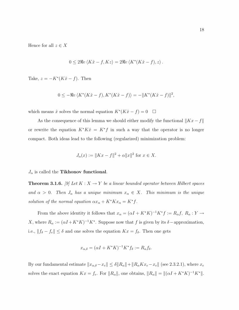
As the consequence of this lemma we should either modify the functional ‖Kx− f‖
or rewrite the equation K∗Kx = K∗f in such a way that the operator is no longer
compact. Both ideas lead to the following (regularized) minimization problem:
Jα(x) := ‖Kx− f‖2 + α‖x‖2 for x ∈ X.
Jα is called the Tikhonov functional.
Theorem 3.1.6. [9] Let K : X → Y be a linear bounded operator between Hilbert spaces
and α > 0. Then Jα has a unique minimum xα ∈ X. This minimum is the unique
solution of the normal equation αxα +K∗Kxα = K∗f .
From the above identity it follows that xα = (αI +K∗K)−1K∗f := Rαf, Rα : Y →
X, where Rα := (αI+K∗K)−1K∗. Suppose now that f is given by its δ−approximation,
i.e., ‖fδ − fe‖ ≤ δ and one solves the equation Kx = fδ. Then one gets
xα,δ = (αI +K∗K)−1K∗fδ := Rαfδ.
By our fundamental estimate ‖xα,δ−xe‖ ≤ δ‖Rα‖+‖RαKxe−xe‖ (see 2.3.2.1), where xe
solves the exact equation Kx = fe. For ‖Rα‖, one obtains, ‖Rα‖ = ‖(αI +K∗K)−1K∗‖.

19
By polar decomposition K = U(K∗K)1/2, where U is a partial isometry:
‖Uq‖ = ‖q‖ for all q ∈ N(U)⊥ and N(U) = {q : Uq = 0}.
Therefore,
‖Rα‖ = ‖(αI +K∗K)−1(K∗K)1/2U‖ ≤ ‖(αI +K∗K)−1(K∗K)1/2‖ := ‖ϕ(A)‖
with A := K∗K. Since A is self-adjoint, by spectral theorem one derives
‖ϕ(A)‖ = supλ∈σ(A)
|f(λ)| = supλ∈σ(A)
√λ
λ+ α=
1
2√α.
Here σ(A) = [0, ‖K‖2]. Thus, δ‖Rα‖ ≤ δ2√α
.
In order to analyze ‖RαKxe − xe‖, we make an additional assumption: xe = K∗z ∈
K∗(Y ), z ∈ Y . Then
‖RαKxe − xe‖ = ‖[K∗K + αI]−1K∗Kxe − xe‖
= ‖[K∗K + αI]−1K∗Kxe − [K∗K + αI]−1[K∗K + αI]xe‖
= ‖[K∗K + αI]−1(K∗Kxe −K∗Kxe − αIxe)‖
= ‖[K∗K + αI]−1(−αIxe)‖ = ‖[K∗K + αI]−1(−αxe)‖
= α‖[K∗K + αI]−1K∗z‖ ≤ α‖[K∗K + αI]−1K∗‖ ‖z‖
≤ α‖z‖2√α
=‖z‖√α
2.
This inequality proves that the operators Rα : Y → X, Rα = (αI + K∗K)−1K∗ form a
regularization strategy with limα→0 ‖RαKxe − xe‖ ≤ limα→0‖z‖√α
2= 0. It is called the
Tikhonov regularization method. Combining the estimates for δ‖Rα‖ and ‖RαKxe−
20
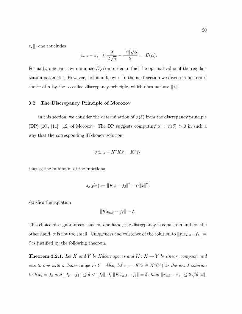
xe‖, one concludes
‖xα,δ − xe‖ ≤δ
2√α
+‖z‖√α
2:= E(α).
Formally, one can now minimize E(α) in order to find the optimal value of the regular-
ization parameter. However, ‖z‖ is unknown. In the next section we discuss a posteriori
choice of α by the so called discrepancy principle, which does not use ‖z‖.
3.2 The Discrepancy Principle of Morozov
In this section, we consider the determination of α(δ) from the discrepancy principle
(DP) [10], [11], [12] of Morozov. The DP suggests computing α = α(δ) > 0 in such a
way that the corresponding Tikhonov solution:
αxα,δ +K∗Kx = K∗fδ
that is, the minimum of the functional
Jα,δ(x) := ‖Kx− fδ‖2 + α‖x‖2,
satisfies the equation
‖Kxα,δ − fδ‖ = δ.
This choice of α guarantees that, on one hand, the discrepancy is equal to δ and, on the
other hand, α is not too small. Uniqueness and existence of the solution to ‖Kxα,δ−fδ‖ =
δ is justified by the following theorem.
Theorem 3.2.1. Let X and Y be Hilbert spaces and K : X → Y be linear, compact, and
one-to-one with a dense range in Y . Also, let xe = K∗z ∈ K∗(Y ) be the exact solution
to Kxe = fe and ‖fe− fδ‖ ≤ δ < ‖fδ‖. If ‖Kxα,δ − fδ‖ = δ, then ‖xα,δ − xe‖ ≤ 2√δ‖z‖.

21
Proof: Since xα,δ minimizes the Tikhonov functional Jα,δ = ‖Kxe − fδ‖2 + α‖xe‖2, we
can conclude that
α‖xα,δ‖2 + δ2 = Jα,δ(xα,δ) ≤ Jα,δ(xe) = α‖xe‖2 + ‖fe − fδ‖2 ≤ α‖xe‖2 + δ2,
and hence ‖xα,δ‖ ≤ ‖xe‖ for all δ > 0. This gives us the following important estimate:
‖xα,δ − xe‖2 = ‖xα,δ‖2 − 2<e 〈xα,δ, xe〉+ ‖xe‖2
≤ 2[‖xe‖2 −<e 〈xα,δ, xe〉] = 2<e 〈xe − xα,δ, xe〉 .
Let xe = K∗z, z ∈ Y . Then
‖xα,δ − xe‖2 ≤ 2<e 〈xe − xα,δ, K∗z〉 = 2<e 〈fe −Kxα,δ, z〉
≤ 2<e 〈fe − fδ, z〉+ 2<e 〈fδ −Kxα,δ, z〉
≤ 2δ‖z‖+ 2δ‖z‖ = 4δ‖z‖.
Therefore, ‖xα,δ − xe‖ ≤ 2√δ‖z‖, as was to be shown.
The condition ‖fδ‖ > δ is reasonable, since otherwise the right-hand side is less than
δ, and one can take xδ = 0. This also shows that the determination of α does not have
to satisfy the equation ‖Kxα,δ − fδ‖ = δ exactly. We can use the following bounds that
will then guarantee the same level of accuracy.
c1δ ≤ ‖Kxα,δ − fδ‖ ≤ c2δ.
How to solve the equation ‖Kxα,δ − fδ‖ = δ? We introduce
ϕ(α) := ‖Kxα,δ − fδ‖2 − δ2.

22
Then the equation ϕ(α) = 0 is equivalent to ‖Kxα,δ − fδ‖ = δ, and it can be solved
numerically for example, by Newton’s method:
αj+1 = αj −ϕ(αj)
ϕ′(αj), j = 0, 1, 2, ....
The derivative ϕ′(α) can be calculated as follows:
ϕ′(α) =
[〈Kxα,δ − fδ, Kxα,δ − fδ〉 − δ2
]′α
=
⟨Kdxα,δdα
,Kxα,δ − fδ⟩
+
⟨Kxα,δ − fδ, K
dxα,δdα
⟩= 2<e
⟨Kdxα,δdα
,Kxα,δ − fδ⟩.
We now computedxα,δdα
by differentiating the identity
αxα,δ +K∗Kxα,δ = K∗fδ
implicitly. Since the right-hand side does not depend on α, one has
xα,δ + αdxα,δdα
+K∗Kdxα,δdα
= 0.
Solving fordxα,δdα
, we get
dxα,δdα
= −[αI +K∗K]−1xα,δ = −[αI +K∗K]−1[αI +K∗K]−1K∗fδ.

23
Substituting this into ϕ′(α), one derives
ϕ′(α) = 2<e⟨−K[αI +K∗K]−1xα,δ, Kxα,δ − fδ
⟩= 2<e
⟨−K[αI +K∗K]−1[αI +K∗K]−1K∗fδ, K[αI +K∗K]−1K∗fδ − fδ
⟩.

24
Chapter 4
NUMERICAL SIMULATIONS
4.1 Statement of the Problem
In this chapter, we will show that as opposed to the ’naive’ discretization used in
section 2.1, the Tikhonov regularization combined with Morozov’s discrepancy principle,
results in a stable numerical solution to an ill-posed integral equation.
To illustrate the efficiency of Tikhonov-Morozov algorithm we consider the same
equation as in Section 2.1:
Kx :=
b∫a
k(t, s)x(s)ds = f(t), [a, b] = [c, d] = [0, 1],
with k(t, s) = ets, K : L2[a, b]→ L2[c, d] and fe(t) =et+1 − 1
t+ 1.
Note that in L2[a, b] the norm is generated by the following inner product:
〈[f ], [g]〉L2 :=
b∫a
f(t)g(t)dt, f ∈ [f ], g ∈ [g],
where [f ], [g] are equivalence classes of functions, i.e., two functions are in the same class
if they only differ on a set of Lebesgue’s measure zero. Also, the number of partitions

25
we will use are n = 4, 8, 16, 32 while varying t ∈ [0, 1] for our tables. Note that K is
self-adjoint, that is K∗ = K. Indeed, since k(t, s) = ets, K∗ would lead to the following,
K∗x :=
d∫c
k(s, t)x(t)dt, where [c, d] = [a, b] = [0, 1].
Then k(s, t) = est. Since t and s are real valued, est = ets. Therefore, K∗ = K.
Table 4.1. Comparison of Errors
‖xe − xα,δ‖, δn = e2h2
3+ σ
n\σ 0.0001 0.05 0.14 0.0876 0.1177 0.14368 0.0298 0.0376 0.040616 0.0052 0.0273 0.037332 0.0005 0.0196 0.0338
Table 4.2. Values of α by Discrepancy Principle
σ n = 4 n = 8 n = 16 n = 320.1 0.173360 0.068038 0.032997 0.0188960.05 0.144455 0.050745 0.022335 0.011284
0.0001 0.109950 0.025159 0.005009 0.001159
We discretize the operator K by again using the trapezoidal rule to approximate the
integral
(Knx)i := h
[1
2x0 +
1
2eihxn +
n−1∑j=1
eijh2
xj
]= (fδ)i,
where xj is an approximate value for x(jh), j = 0, ..., n, and (fδ)i = f(ih), i = 0, ..., n,
is a noisy right-hand side. Then for the discrete analog of the Tikhonov solution, one

26
gets
xα,δ = (αIn +K∗nKn)−1K∗nfδ, K∗n = Kn.
In order to implement the discrepancy principle, one has to solve the following nonlinear
equation:
ϕ(α) := ‖Knxα,δ − fδ‖2 − δ2 = 0.
Introduce the notation of
Gn := (αIn +K∗nKn)−1.
Substituting xα,δ = GnK∗nfδ in the expression for ϕ(α), one concludes
ϕ(α) := ‖KnGnK∗nfδ − fδ‖2 − δ2 := ‖(KnGnK
∗n − In)fδ‖2 − δ2 = 0.
Table 4.3. Comparative Results for σ = 0.0001
xe − xα,δt n = 4 n = 8 n = 16 n = 32 xe = exp(t)0 -0.1852 -0.1845 -0.0803 -0.0134 1.00
0.25 -0.0912 -0.1220 -0.0616 -0.0193 1.280.50 0.0444 -0.0262 -0.0235 -0.0138 1.650.75 0.2355 0.1148 0.0424 0.0094 2.121.00 0.5003 0.3169 0.1476 0.0589 2.72
We solve ϕ(α) = 0 by Newton’s method:
αj+1 = αj −ϕ(αj)
ϕ′(αj), j = 0, 1, ... .

27
Figure 4.1. Exact and Approximate Solutions for σ = 0.0001
As it has been shown in the previous section,
ϕ′(α) = 2
⟨Kn
dxα,δdα
, Knxα,δ − fδ⟩.
Recall, that the operator in our example is real-valued. Besides,
dxα,δdα
= −Gnxα,δ = −G2nK∗nfδ.
Hence,
ϕ′(α) = −2⟨KnG
2nK∗nfδ, KnGnK
∗nfδ − fδ
⟩= −2
⟨KnG
2nKnfδ, (KnGnKn − In)fδ
⟩,

28
since K∗n = Kn. We terminate Newton’s method when
|αj+1 − αj| < 10−6 and |ϕ(αj)| < 10−6,
which is comparable to the Matlab solver ’fsolve’.
Table 4.4. Comparative Results for σ = 0.05
xe − xα,δt n = 4 n = 8 n = 16 n = 32 xe = exp(t)0 -0.1980 -0.1868 -0.2004 -0.1838 1.00
0.25 -0.0880 -0.1153 -0.1344 -0.1274 1.280.50 0.0678 -0.0080 -0.0338 -0.0396 1.650.75 0.2845 0.1479 0.1139 0.0917 2.121.00 0.5816 0.3691 0.3254 0.2826 2.72
4.2 Sources of Noise
Table 4.5. Comparative Results for σ = 0.1
xe − xα,δt n = 4 n = 8 n = 16 n = 32 xe = exp(t)0 -0.2027 -0.1776 -0.2302 -0.2429 1.00
0.25 -0.0815 -0.1040 -0.1502 -0.1634 1.280.50 0.0888 0.0061 -0.0312 -0.0449 1.650.75 0.3236 0.1653 0.1407 0.1266 2.121.00 0.6435 0.3906 0.3835 0.3698 2.72
To generate fδ, we add a noise term to the exact function fe. That noise term

29
Figure 4.2. Exact and Approximate Solutions for σ = 0.05
Figure 4.3. Exact and Approximate Solutions for σ = 0.1
30
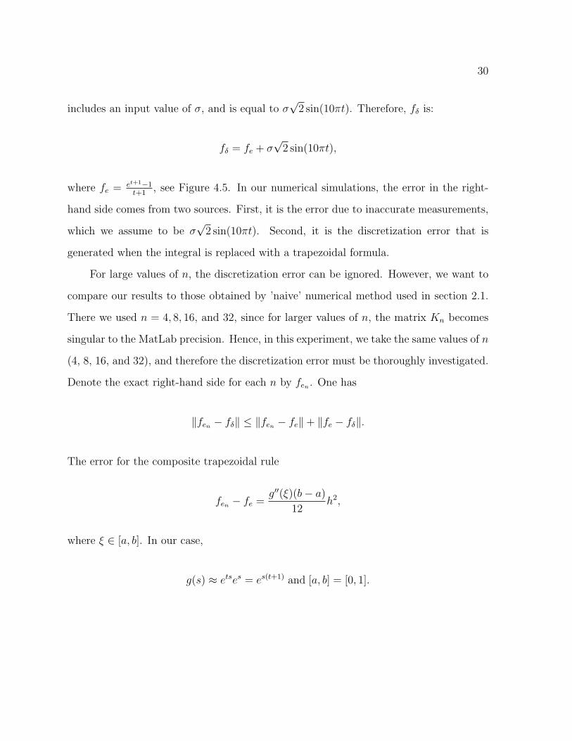
includes an input value of σ, and is equal to σ√
2 sin(10πt). Therefore, fδ is:
fδ = fe + σ√
2 sin(10πt),
where fe = et+1−1t+1
, see Figure 4.5. In our numerical simulations, the error in the right-
hand side comes from two sources. First, it is the error due to inaccurate measurements,
which we assume to be σ√
2 sin(10πt). Second, it is the discretization error that is
generated when the integral is replaced with a trapezoidal formula.
For large values of n, the discretization error can be ignored. However, we want to
compare our results to those obtained by ’naive’ numerical method used in section 2.1.
There we used n = 4, 8, 16, and 32, since for larger values of n, the matrix Kn becomes
singular to the MatLab precision. Hence, in this experiment, we take the same values of n
(4, 8, 16, and 32), and therefore the discretization error must be thoroughly investigated.
Denote the exact right-hand side for each n by fen . One has
‖fen − fδ‖ ≤ ‖fen − fe‖+ ‖fe − fδ‖.
The error for the composite trapezoidal rule
fen − fe =g′′(ξ)(b− a)
12h2,
where ξ ∈ [a, b]. In our case,
g(s) ≈ etses = es(t+1) and [a, b] = [0, 1].
31
Thus,
‖fen − fe‖ =
( 1∫0
(t+ 1)4e2(t+1)h4
122dt
) 12
≤ h2
12
( 1∫0
24e4dt
) 12
=e2h2
3, since t ∈ [0, 1].
One can also see that
‖fe − fδ‖2 = 2
1∫0
σ2 sin2(10πt)dt = 2σ2
1∫0
1− cos(20πt)
2dt = 2σ2 1
2= σ2.
Hence, ‖fen − fδ‖ ≤ e2h2
3+ σ := δn. Note that δn changes as n changes since h, the step
size, is dependent on n, the number of partitions. We use the L2-norm instead of the
infinity-norm since the discrepancy principle of Morozov is justified for Hilbert spaces.
The discrete analog of this norm is used to compute ϕ(α) in the Newton method for the
same reason.
4.3 Simulation
For the experiment, we apply the discrepancy principle with σ = 0.1, σ = 0.05, and
σ = 0.0001. As α0, the initial approximation, we take 14, because ϕ(0) < 0 and ϕ(1
2) > 0.
The first Table 4.1 shows a comparison of the norms and confirms that as n gets larger
we have convergence to the exact solution for xe.
The second Table 4.2, shows α versus σ for different values of n. Note that σ = 0
is not included in the table since we would only have the discretization error of the
trapezoidal rule (as done in Table 2.1). One can see in the Table 4.2, as the noise
gets smaller, α also gets smaller, as to be expected. After evaluating α by Morozov’s
discrepancy principle, we can now find xα,δ and compare it to our exact value of xe = et
for σ = 0.1, 0.05, 0.0001, and n = 4, 8, 16, 32. Table 4.3 shows how xα,δ differs from
32
Figure 4.4. Exact and Approximate Solutions for n = 32
Figure 4.5. Exact and Approximate Values of Right-hand Side

33
xe for σ = 0.0001, our smallest value for σ, Figure 4.1 is the corresponding picture. As
you can see, as n gets larger, the approximation converges towards the exact solution as
guaranteed by the convergence theorem. Table 4.4 and Figure 4.2 show a similar result
for σ = 0.05, as does Table 4.5 and Figure 4.3 for σ = 0.1, our largest σ. One can see
that when σ is small we get a much better approximation of our exact solution. The
final Figure 4.4 compares the exact and approximate solutions for various σ and n = 32.
Again when n = 32 and σ = 0.0001 the approximation is the best.
In conclusion, this part of the experiment worked as the general theory said. We did
have to use careful consideration of the error term since our n was so small. The general
theory tends toward a larger n and therefore does not consider what an important role
this term can play for a very small number of partitions such as we used. The next
chapter will compare our regularized version of the integral to our naive discretization
used in chapter 2.

34
Chapter 5
DISCUSSION
5.1 Summary
For our summary we are using σ = 0.05 as part of the noise in the Tikhonov regular-
ization with Morozov’s discrepancy since it is the middle of the three that we choose to
work with. We start by comparing the two tables, Table 5.1 for our ’naive’ discretization
and Table 5.2 for the Tikhonov-Morozov algorithm. Note that for the ’naive’ discretiza-
tion, σ = 0, and the only noise is due to finite-dimensional approximatation for the
integral. As one can see, the numerical solutions obtained by the Tikhonov-Morozov
algorithm are much better than those done by the ’naive’ discretization. The errors for
each n show that while the ’naive’ discretization oscillates wildly and gets worse as n
increases, the Tikhonov-Morozov algorithm actually gets better as n gets larger. This is
confirmed by the general theory.
We now move to the figures. Again Figure 5.1 refers to the ’naive’ discretization
while Figure 5.2 refers to the Tikhonov-Morozov algorithm. As foretold in the tables,
the ’naive’ discretization varies wildly while the Tikhonov-Morozov algorithm generates
a smooth line that converges toward the exact value as n gets larger. All of the values
of n could not even be shown in the ’naive’ discretization due to the fact that at n = 16
and n = 32 the matrix is nearly singular and does not return a better result but a much

35
Table 5.1. Results for the ’Naive’ Discretization
x(ti)− xit n = 4 n = 8 n = 16 n = 32 x(ti) = exp(ti)0 0.56 0.53 -3.20 -31.14 1.00
0.25 1.95 -0.74 45.30 13.40 1.280.50 0.69 -3.11 24.17 -12.32 1.650.75 3.13 -0.95 66.94 33.04 2.121.0 1.63 1.49 -0.72 -9.83 2.72
Table 5.2. Comparative Results for σ = 0.05
xe − xα,δt n = 4 n = 8 n = 16 n = 32 xe = exp(t)0 -0.1980 -0.1868 -0.2004 -0.1838 1.00
0.25 -0.0880 -0.1153 -0.1344 -0.1274 1.280.50 0.0678 -0.0080 -0.0338 -0.0396 1.650.75 0.2845 0.1479 0.1139 0.0917 2.121.00 0.5816 0.3691 0.3254 0.2826 2.72
worse one. Note that even thought we are showing σ = 0.05 as our representative for
Tikhonov-Morozov algorithm, the one with σ = 0.1, our largest value for σ, is still much
better approximation than the naive discretization, which uses σ = 0.
5.2 Advantages
There are definite advantages to using the Tikhonov regularization with Morozov’s
discrepancy principle. The first and most obvious is that it returns a much better approx-
imate solution than the ’naive’ discretization does. While using the same trapezoidal rule
for the approximation of the integral, the relatively simple regularization by the Tikhonov
method along with Morozov’s discrepancy principle produces little to no discernible error

36
Figure 5.1. Exact and Approximate Solutions
Figure 5.2. Exact and Approximate Solution for σ = 0.05

37
as the partitions get sufficiently large, meaning you get a much closer approximation as
the number of partitions gets larger for any amount of noise. In other words, the accuracy
of the regularized solutions gets better as n approaches infinity, which is not the case for
the ’naive’ discretization.
5.3 Disadvantages
The biggest disadvantage of Tikhonov regularization with Morozov’s discrepancy
principle is the repeated matrix manipulation done to compute the solution. Since the
approximate solution uses the inverse of (αjI + K∗K) one has to make sure that it
exists for every j and to start Newton’s iterations with an overestimate of α rather than
underestimate.
Another disadvantage of Tikhonov regularization is the over-smoothing effect. In
order to reconstruct nonsmooth or discontinuous solutions, one has to use a different
penalty term.

38
REFERENCES
[1] A. Bakushinsky, A.Goncharsky, Ill-posed problem theory and application, Kluver,Dordrecht, 1994.
[2] J. Demmel, Applied Numerical Linear Algebra, Society for Industrial and AppliedMathematics (SIAM), Philidephia, 1997.
[3] H. Engl, M.Hanke, A.Neubauer, Regularization of inverse problems, Kluwer, Dor-drecht, 1996.
[4] James F. Epperson, An Introduction to Numerical Methods and Analysis, JohnWiley & Sons, Inc., 2002, New York.
[5] C.W. Groetsch, The theory of Tikhonov regularization for Fredholm equations ofthe first kind, Pitman, Boston, 1984.
[6] J. Hadamard, Lectures on the Cauchy Problem in Linear Partial Differential Equa-tions, Yale University Press, New Haven, 1923.
[7] M. Hanke, Accelerated Landweber iterations for the solution of Ill-Posed equations,Numer. Math., 60 (1991) 341-373.
[8] B. Hofmann, Regularization of Applied Inverse and Ill-Posed Problems, Teubner,Leipzig, 1986.
[9] A. Kirsch, An Introduction to the Mathematical Theory of Inverse Problems,Springer-Verlag New York, Inc., New York, NY, 1996.
[10] V.A. Morozov Choice of a parameter for the solution of functional equations by theregularization method, Sov. Math. Doklady, 8: 1000-1003, 1967.
[11] V.A. Morozov The error principle in the solution of operational equations by theregularization method, USSR Comput. Math. Math. Phys., 8:63-87, 1968.
[12] V.A. Morozov Methods for Solving Incorrectly Posed Problems, Springer-Verlag,Berlin, 1984.
[13] V.A. Morozov The principle of discrepancy in the solution of inconsistent equa-tions by Tikhonov’s regularization method, Zhurnal Vychislitel’noy matematiky imatematicheskoy fisiki, 13, (1973) 5.
[14] D.L. Phillips, A technique for the numerical solution of certain integral equation ofthe first kind, J. Assoc. Comput. Machinery. 9(1) (1962), 84-97.

39
[15] A.N. Tikhonov, The solution of ill-posed problems, Doklady Akad. Nauk SSSR,151, (1963) 3
[16] A. Tikhonov, A.Leonov, A.Yagola, Nonlinear ill-posed problems, Chapman andHall, London, 1998.
[17] G. Vainikko, A.Veretennikov, Iterative procedures in ill-posed problems, Moscow,Nauka, 1986.
[18] V.V. Vasin, A.L.Ageev, Ill-posed problems with a priori information, VNU, Utrecht,1995.

40
APPENDIX A
% This program is written by MaryGeorge Whitney
%
% This program solves a linear system for an inverse problem
% by using the trapizoidal rule to approximate the integral
%
% The integral is e^ts x(s) ds = f(t)
% Where f(t) = (e^(t+1) - 1)/(t+1)
% The exact value of x = exp(t)
%
%%%%%%%%%%%%%%%%%%%%%%%%%%%%%%%%%%%%%%%%%%%%%%%%%%%%%%%%%%%%%%%%
%
% Variable List
%
%%%%%%%%%%%%%%%%%%%%%%%%%%%%%%%%%%%%%%%%%%%%%%%%%%%%%%%%%%%%%%%%
%
% K - matrix for the integral answers
% B - array matrix for the approximation for chart
% check - while loop variable
% ck - while loop variable
% E - array matrix for the exact values
% m - inline function for the right hand side of equation
% g - inline finction for the exact value of x
% h - subinterval = 1/n
% i - looping variable for the t partition
% j - looping variable for the s partition
% n - number of subintervals - input by user
% N - the number of subintervals plus 1 for matrix reference
% R - array matrix for error
% s - partition variable = j*h
% t - partition variable = i*h
% w - input variable for repeating program
% x - array matrix for the approximated answer of K\f
% f - array matrix for the solution answers
%
%%%%%%%%%%%%%%%%%%%%%%%%%%%%%%%%%%%%%%%%%%%%%%%%%%%%%%%%%%%%%%%%

41
%
% Main Program
%
%%%%%%%%%%%%%%%%%%%%%%%%%%%%%%%%%%%%%%%%%%%%%%%%%%%%%%%%%%%%%%%%
clc;
check = 0;
while check == 0
% Introduction and input of number of intervals
fprintf(’This program solves a liner system for an inverse problem.\n’);
fprintf(’It uses the trapizoidal rule to approximate the integral:\n’);
fprintf(’e^ts x(s) ds = f(t) the integral goes from 0 to 1\n’);
fprintf(’Please enter the number of partitions desired:\n’);
n = input(’ ’);
% Initalize variables
ck = 0;
h = 1/n;
N = n + 1;
K = zeros(N,N);
f = zeros(N,1);
E = zeros(N,1);
x = zeros(N,1);
B = zeros(N,1);
R = zeros(N,1);
m = inline (’(exp(t+1) - 1)/(t+1)’);
g = inline (’exp (t)’);
% Build matrices
for i=1:N
t = (i-1)*h;
f(i) = m(t);
E(i) = g(t);
for j=1:N
s = (j-1)*h;
K(i,j) = exp(t*s);
end % ends j loop
end % ends i loop
%Finish off the K matrix

42
K(:,1) = K(:,1)/2;
K(:,N) = K(:,N)/2;
K = h*K;
% Build solution
x = K\f;
% Build matrix for print chart
for i=1:N
t = (i-1)*h;
switch t
case 0
B(i) = x(i);
R(i) = E(i) - x(i);
case .25
B(i) = x(i);
R(i) = E(i) - x(i);
case .5
B(i) = x(i);
R(i) = E(i) - x(i);
case .75
B(i) = x(i);
R(i) = E(i) - x(i);
case 1
B(i) = x(i);
R(i) = E(i) - x(i);
otherwise
B(i) = 0;
R(i) = 0;
end % ends switch
end % ends for i
%Print selected solutions
fprintf(’Remember that the number of partitions is: %3.0f \n’, n);
for i=1:N
if B(i) ~= 0
t = (i-1)*h;
fprintf(’t = %3.2f\n’, t);
fprintf(’Our approximation is %5.2f\n’, B(i));
fprintf(’Our exact value is %5.2f\n’, E(i));
fprintf(’With an error of %5.2f.\n\n’,R(i));

43
end % ends if
end % ends for
%Plotting the compairison
i=1:N;
q=(i-1)/n;
plot(q,g(q),’ro-’,q,x(i),’bd:’);
axis auto;
title(’Exact and approximate functions’);
xlabel(’step size’);
legend(’Exact’,’Approximation’,’Location’,’NorthWest’);
while ck == 0
fprintf(’Would you like to run again?\n’);
fprintf(’Please type ’’y’’ or ’’n’’.\n’);
w = input(’ ’,’s’);
fprintf(’\n\n\n’);
switch lower(w)
case ’y’
check = 0;
ck = 1;
case ’n’
check = 1;
ck = 1;
otherwise
fprintf(’Please try again’);
check = 0;
ck = 0;
end % ends switch
end % ends while ck loop
end % ends while check loop

44
APPENDIX B
Exercise1
This program solves a liner system for an inverse problem.
It uses the trapizoidal rule to approximate the integral:
e^ts x(s) ds = f(t) the integral goes from 0 to 1
Please enter the number of partitions desired:
4
Remember that the number of partitions is: 4
t = 0.00
Our approximation is 0.56
Our exact value is 1.00
With an error of 0.44.
t = 0.25
Our approximation is 1.95
Our exact value is 1.28
With an error of -0.67.
t = 0.50
Our approximation is 0.69
Our exact value is 1.65
With an error of 0.95.
t = 0.75
Our approximation is 3.13
Our exact value is 2.12
With an error of -1.02.
t = 1.00
Our approximation is 1.63
Our exact value is 2.72
With an error of 1.09.
Would you like to run again?
Please type ’y’ or ’n’.
y

45
This program solves a liner system for an inverse problem.
It uses the trapizoidal rule to approximate the integral:
e^ts x(s) ds = f(t) the integral goes from 0 to 1
Please enter the number of partitions desired:
8
Remember that the number of partitions is: 8
t = 0.00
Our approximation is 0.53
Our exact value is 1.00
With an error of 0.47.
t = 0.25
Our approximation is -0.74
Our exact value is 1.28
With an error of 2.02.
t = 0.50
Our approximation is -3.11
Our exact value is 1.65
With an error of 4.76.
t = 0.75
Our approximation is -0.95
Our exact value is 2.12
With an error of 3.07.
t = 1.00
Our approximation is 1.49
Our exact value is 2.72
With an error of 1.23.
Would you like to run again?
Please type ’y’ or ’n’.
y
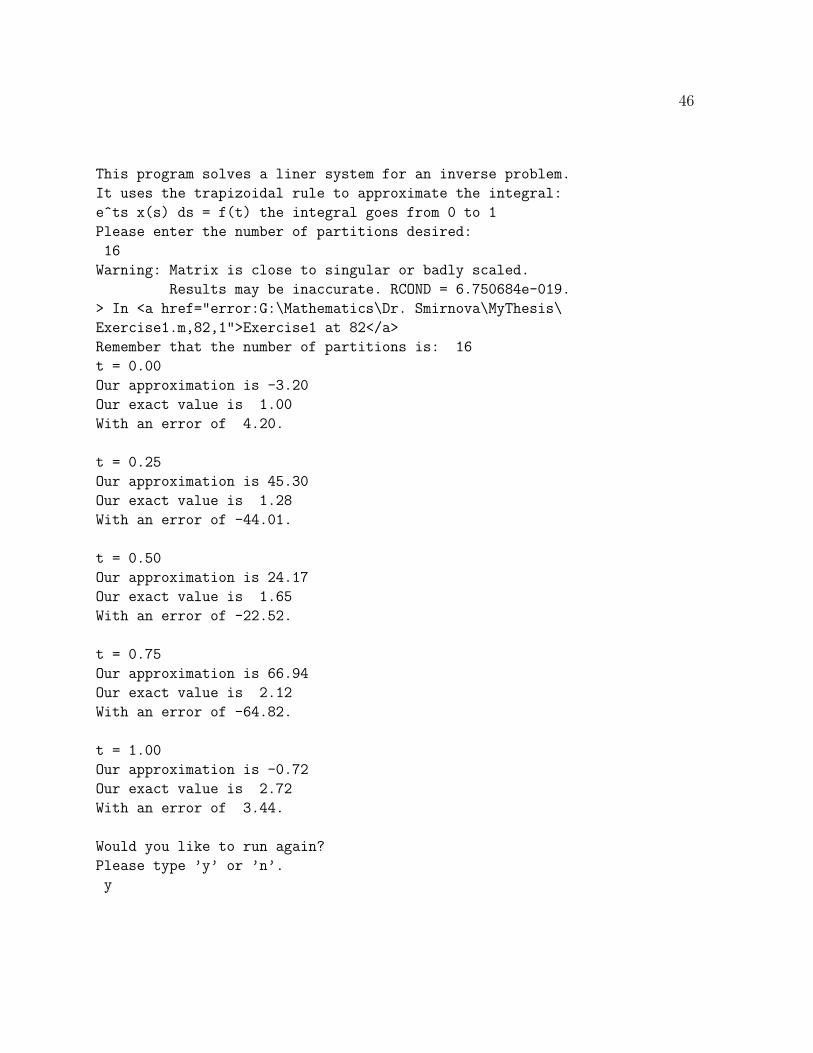
46
This program solves a liner system for an inverse problem.
It uses the trapizoidal rule to approximate the integral:
e^ts x(s) ds = f(t) the integral goes from 0 to 1
Please enter the number of partitions desired:
16
Warning: Matrix is close to singular or badly scaled.
Results may be inaccurate. RCOND = 6.750684e-019.
> In <a href="error:G:\Mathematics\Dr. Smirnova\MyThesis\
Exercise1.m,82,1">Exercise1 at 82</a>
Remember that the number of partitions is: 16
t = 0.00
Our approximation is -3.20
Our exact value is 1.00
With an error of 4.20.
t = 0.25
Our approximation is 45.30
Our exact value is 1.28
With an error of -44.01.
t = 0.50
Our approximation is 24.17
Our exact value is 1.65
With an error of -22.52.
t = 0.75
Our approximation is 66.94
Our exact value is 2.12
With an error of -64.82.
t = 1.00
Our approximation is -0.72
Our exact value is 2.72
With an error of 3.44.
Would you like to run again?
Please type ’y’ or ’n’.
y

47
This program solves a liner system for an inverse problem.
It uses the trapizoidal rule to approximate the integral:
e^ts x(s) ds = f(t) the integral goes from 0 to 1
Please enter the number of partitions desired:
32
Warning: Matrix is close to singular or badly scaled.
Results may be inaccurate. RCOND = 2.697308e-019.
> In <a href="error:G:\Mathematics\Dr. Smirnova\MyThesis
\Exercise1.m,82,1">Exercise1 at 82</a>
Remember that the number of partitions is: 32
t = 0.00
Our approximation is -31.14
Our exact value is 1.00
With an error of 32.14.
t = 0.25
Our approximation is 13.04
Our exact value is 1.28
With an error of -11.76.
t = 0.50
Our approximation is -12.32
Our exact value is 1.65
With an error of 13.97.
t = 0.75
Our approximation is 33.04
Our exact value is 2.12
With an error of -30.92.
t = 1.00
Our approximation is -9.83
Our exact value is 2.72
With an error of 12.55.
Would you like to run again?
Please type ’y’ or ’n’.
n

48
APPENDIX C
% This program was written by MaryGeorge L. Whitney
% It is part of a master thesis project under the direction of
% Dr. Alexandria Smirnova
%
% This program uses Newton’s method to produce a regularization
% strategy for an ill-posed integral problem
%
%%%%%%%%%%%%%%%%%%%%%%%%%%%%%%%%%%%%%%%%%%%%%%%%%%%%%%%%%%%%%%%%%%%%%%%%%
%
% Variable List
%
%%%%%%%%%%%%%%%%%%%%%%%%%%%%%%%%%%%%%%%%%%%%%%%%%%%%%%%%%%%%%%%%%%%%%%%%%
%
% alpha0 - inital value (approximation) for alpha used in regularization
% alpha1 - scalar for regularization
% alphaTol - tolerance used for alpha
% cek - while loop variable
% check - while loop variable
% choice - input variable for continuation
% ck - while loop variable
% sigma - input variable, noise, noted as sigma in the text
% fe - array variable, right-hand side exact
% fdelta - array variable, noisy right-hand side
% g - inline function, calculates exact x
% h - step size
% i - loop variable
% I - matrix variable, identity matrix
% j - loop variable
% K - matrix variable, integral from our equation
% Kstar - matrix variable, Hermitian matrix of K
% m - inline function, calculates right-hand side (fe)
% n - input variable, number of partitions
% N - number of partitions plus one for matrices
% phi - regularization equation based on alpha, return value from Newton’s

49
% phiprime - derivative of phi, return value from Newton’s
% phiTol - used to check tolerance of phi
% q - plot variable
% R - array variable, error difference for xe and xalphadelta
% s - partition variable j*h
% t - partition variable i*h
% tol - tolerance allowed
% w - inline function for noisy right-hand side (fdelta)
% xalphadelta - array variable, regualized noisy answer to Kx=f
% xexact - array variable, exact answer to Kx=f
% G - matrix variable, used for alpha calculation (alpha*I+K*K)^-1
%
%%%%%%%%%%%%%%%%%%%%%%%%%%%%%%%%%%%%%%%%%%%%%%%%%%%%%%%%%%%%%%%%%%%%%%%%
%
% Main Program
%
%%%%%%%%%%%%%%%%%%%%%%%%%%%%%%%%%%%%%%%%%%%%%%%%%%%%%%%%%%%%%%%%%%%%%%%%
clc;
check = 0;
while check == 0 %loop for the program
cek = 0;
% Input noise: sigma and number of partitions: n
while cek == 0
fprintf(’Please enter the amount of noise.\n’);
fprintf(’This is sigma in our problem.\n’);
fprintf(’Sigma must be > 0 and < 1.\n’);
sigma = input(’ ’);
fprintf(’\n’);
if (sigma < 0) | (sigma > 1)
fprintf(’Please try again. Sigma is out of range.\n’);
else
cek = 1;
end % Ends sigma range check
end % ends while loop for delta
fprintf(’Please enter the number of partitions.\n’);
n = input(’ ’);
fprintf(’\n \n \n’);

50
% Initialize variables and inline functions
N = n+1;
h = 1/n;
I = eye(N);
t = 0;
fe = zeros(N,1);
fdelta = zeros(N,1);
xexact = zeros(N,1);
s = 0;
K = zeros(N,N);
Kstar = zeros(N,N);
alpha0 = .25; %inital approximation for alpha
alphaTol = 1; %inital tolerance for alpha
phiTol = 1; %inital tolerance for phi
tol = 10^(-6); % tolerance level
G = zeros(N,N);
phi = 0;
phiprime = 0;
alpha1 = 0;
xalphadelta = zeros(N,1);
R = zeros(N,1);
q = 0;
m = inline(’(exp(t+1)-1)/(t+1)’); %inline function for f-exact
g = inline(’exp(t)’); %inline function for exact x
w = inline(’(exp(t+1)-1)/(t+1) + sigma *sqrt(2)* sin(10*pi*t)’, ’sigma’, ’t’); %function for f-delta
% Build matrix K
%Trapezoidal rule for integral
for i = 1:N
t = (i-1)*h;
fe(i) = m(t);
fdelta(i) = w(sigma,t);
xexact(i) = g(t);
for j = 1:N
s = (j-1)*h;
K(i,j) = exp(t*s);
end %end for j loop
end %end for i loop
K(:,1) = K(:,1)/2;
K(:,N) = K(:,N)/2;
51
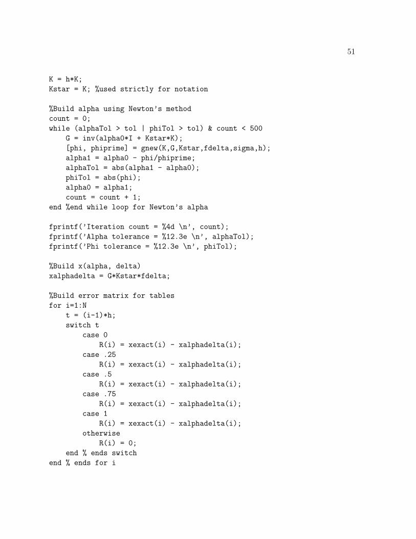
K = h*K;
Kstar = K; %used strictly for notation
%Build alpha using Newton’s method
count = 0;
while (alphaTol > tol | phiTol > tol) & count < 500
G = inv(alpha0*I + Kstar*K);
[phi, phiprime] = gnew(K,G,Kstar,fdelta,sigma,h);
alpha1 = alpha0 - phi/phiprime;
alphaTol = abs(alpha1 - alpha0);
phiTol = abs(phi);
alpha0 = alpha1;
count = count + 1;
end %end while loop for Newton’s alpha
fprintf(’Iteration count = %4d \n’, count);
fprintf(’Alpha tolerance = %12.3e \n’, alphaTol);
fprintf(’Phi tolerance = %12.3e \n’, phiTol);
%Build x(alpha, delta)
xalphadelta = G*Kstar*fdelta;
%Build error matrix for tables
for i=1:N
t = (i-1)*h;
switch t
case 0
R(i) = xexact(i) - xalphadelta(i);
case .25
R(i) = xexact(i) - xalphadelta(i);
case .5
R(i) = xexact(i) - xalphadelta(i);
case .75
R(i) = xexact(i) - xalphadelta(i);
case 1
R(i) = xexact(i) - xalphadelta(i);
otherwise
R(i) = 0;
end % ends switch
end % ends for i

52
%Print selected solutions
fprintf(’Our sigma is: %5.4f \n’, sigma);
fprintf(’The number of partitions is: %3.0f \n’, n);
for i=1:N
if R(i) ~= 0
t = (i-1)*h;
fprintf(’t = %3.2f \n’, t);
fprintf(’alpha = %7.6f \n’, alpha0);
fprintf(’Our approximation is %5.4f\n’, xalphadelta(i));
fprintf(’Our exact value is %5.4f\n’, xexact(i));
fprintf(’With an error of %5.4f.\n\n’,R(i));
end % ends if
end % ends for
%Plotting the compairison
i=1:N;
q=(i-1)*h;
plot(q,xexact(i),’ro-’,q,xalphadelta(i),’bd:’);
axis auto;
title(’Exact and approximate functions’);
xlabel(’step size’);
legend(’Exact solution xexact(i)’,’Approximate solution xalphadelta(i)’,’Location’,’NorthWest’);
ck = 0;
while ck == 0
fprintf(’Would you like to run again?\n’);
fprintf(’Please type ’’y’’ or ’’n’’.\n’);
choice = input(’ ’,’s’);
fprintf(’\n\n\n’);
switch lower(choice)
case ’y’
check = 0;
ck = 1;
case ’n’
check = 1;
ck = 1;
otherwise
fprintf(’Please try again’);
check = 0;
ck = 0;
end % ends switch

53
end % ends while loop for another run
end % ends while for program loop

54
APPENDIX D
function [y1, y2] = gnew(K,G,Kstar,fdelta,sigma,h);
%%%%%%%%%%%%%%%%%%%%%%%%%%%%%%%%%%%%%%%%%%%%%%%%%%%%%%%%%%%%%%%%%%%%%%%%
% This program is written by MaryGeorge Whitney
% It is the Newton method for Phi and Phiprime
% It uses a special norm for compact Hilbert spaces
%
% Inputs: K - integral matrix
% Kstar - equal to K - used as notation
% G - inverse matrix for (alpha * I + Kstar * K)
% fdelta - noisy right-hand side
% sigma - input noise
% h - tep size
%
%Outputs: Phi at alpha
% Phiprime at alpha
%%%%%%%%%%%%%%%%%%%%%%%%%%%%%%%%%%%%%%%%%%%%%%%%%%%%%%%%%%%%%%%%%%%%%%%%
% Calculate y1 that is phi
z = K*G*Kstar*fdelta - fdelta;
y1 = (z’*z)*h - (sigma00 + exp(2) * (h^2)/3)^2;
%Calculate y2 that is phiprime
a=-K*G*G*Kstar*fdelta;
b=K*G*Kstar*fdelta-fdelta;
y2 = 2*a’*b;

55
APPENDIX E
Exer2
Please enter the amount of noise.
This is sigma in our problem.
Sigma must be > 0 and < 1.
.1
Please enter the number of partitions.
4
Iteration count = 39
Alpha tolerance = 4.062e-007
Phi tolerance = 9.396e-007
Our sigma is: 0.1000
The number of partitions is: 4
t = 0.00
alpha = 0.173860
Our approximation is 1.2027
Our exact value is 1.0000
With an error of -0.2027.
t = 0.25
alpha = 0.173860
Our approximation is 1.3655
Our exact value is 1.2840
With an error of -0.0815.
t = 0.50
alpha = 0.173860
Our approximation is 1.5600
Our exact value is 1.6487
With an error of 0.0888.
t = 0.75
alpha = 0.173860

56
Our approximation is 1.7934
Our exact value is 2.1170
With an error of 0.3236.
t = 1.00
alpha = 0.173860
Our approximation is 2.0748
Our exact value is 2.7183
With an error of 0.6435.
Would you like to run again?
Please type ’y’ or ’n’.
y
Please enter the amount of noise.
This is sigma in our problem.
Sigma must be > 0 and < 1.
.1
Please enter the number of partitions.
8
Iteration count = 87
Alpha tolerance = 4.903e-007
Phi tolerance = 9.619e-007
Our sigma is: 0.1000
The number of partitions is: 8
t = 0.00
alpha = 0.068038
Our approximation is 1.1776
Our exact value is 1.0000
With an error of -0.1776.
t = 0.25
alpha = 0.068038
Our approximation is 1.3880
Our exact value is 1.2840
With an error of -0.1040.

57
t = 0.50
alpha = 0.068038
Our approximation is 1.6426
Our exact value is 1.6487
With an error of 0.0061.
t = 0.75
alpha = 0.068038
Our approximation is 1.9517
Our exact value is 2.1170
With an error of 0.1653.
t = 1.00
alpha = 0.068038
Our approximation is 2.3277
Our exact value is 2.7183
With an error of 0.3906.
Would you like to run again?
Please type ’y’ or ’n’.
y
Please enter the amount of noise.
This is sigma in our problem.
Sigma must be > 0 and < 1.
.1
Please enter the number of partitions.
16
Iteration count = 179
Alpha tolerance = 4.998e-007
Phi tolerance = 9.491e-007
Our sigma is: 0.1000
The number of partitions is: 16
t = 0.00
alpha = 0.032997
Our approximation is 1.2302
Our exact value is 1.0000

58
With an error of -0.2302.
t = 0.25
alpha = 0.032997
Our approximation is 1.4342
Our exact value is 1.2840
With an error of -0.1502.
t = 0.50
alpha = 0.032997
Our approximation is 1.6799
Our exact value is 1.6487
With an error of -0.0312.
t = 0.75
alpha = 0.032997
Our approximation is 1.9763
Our exact value is 2.1170
With an error of 0.1407.
t = 1.00
alpha = 0.032997
Our approximation is 2.3348
Our exact value is 2.7183
With an error of 0.3835.
Would you like to run again?
Please type ’y’ or ’n’.
y
Please enter the amount of noise.
This is sigma in our problem.
Sigma must be > 0 and < 1.
.1
Please enter the number of partitions.
32
Iteration count = 360
59
Alpha tolerance = 4.622e-007
Phi tolerance = 9.974e-007
Our sigma is: 0.1000
The number of partitions is: 32
t = 0.00
alpha = 0.018896
Our approximation is 1.2429
Our exact value is 1.0000
With an error of -0.2429.
t = 0.25
alpha = 0.018896
Our approximation is 1.4474
Our exact value is 1.2840
With an error of -0.1634.
t = 0.50
alpha = 0.018896
Our approximation is 1.6936
Our exact value is 1.6487
With an error of -0.0449.
t = 0.75
alpha = 0.018896
Our approximation is 1.9904
Our exact value is 2.1170
With an error of 0.1266.
t = 1.00
alpha = 0.018896
Our approximation is 2.3485
Our exact value is 2.7183
With an error of 0.3698.
Would you like to run again?
Please type ’y’ or ’n’.
y
Please enter the amount of noise.

60
This is sigma in our problem.
Sigma must be > 0 and < 1.
.05
Please enter the number of partitions.
4
Iteration count = 40
Alpha tolerance = 4.719e-007
Phi tolerance = 9.466e-007
Our sigma is: 0.0500
The number of partitions is: 4
t = 0.00
alpha = 0.144455
Our approximation is 1.1980
Our exact value is 1.0000
With an error of -0.1980.
t = 0.25
alpha = 0.144455
Our approximation is 1.3721
Our exact value is 1.2840
With an error of -0.0880.
t = 0.50
alpha = 0.144455
Our approximation is 1.5809
Our exact value is 1.6487
With an error of 0.0678.
t = 0.75
alpha = 0.144455
Our approximation is 1.8325
Our exact value is 2.1170
With an error of 0.2845.
t = 1.00
alpha = 0.144455
Our approximation is 2.1367
Our exact value is 2.7183
With an error of 0.5816.

61
Would you like to run again?
Please type ’y’ or ’n’.
y
Please enter the amount of noise.
This is sigma in our problem.
Sigma must be > 0 and < 1.
.05
Please enter the number of partitions.
8
Iteration count = 88
Alpha tolerance = 5.879e-007
Phi tolerance = 8.928e-007
Our sigma is: 0.0500
The number of partitions is: 8
t = 0.00
alpha = 0.050745
Our approximation is 1.1868
Our exact value is 1.0000
With an error of -0.1868.
t = 0.25
alpha = 0.050745
Our approximation is 1.3993
Our exact value is 1.2840
With an error of -0.1153.
t = 0.50
alpha = 0.050745
Our approximation is 1.6567
Our exact value is 1.6487
With an error of -0.0080.
t = 0.75
alpha = 0.050745
Our approximation is 1.9691

62
Our exact value is 2.1170
With an error of 0.1479.
t = 1.00
alpha = 0.050745
Our approximation is 2.3492
Our exact value is 2.7183
With an error of 0.3691.
Would you like to run again?
Please type ’y’ or ’n’.
y
Please enter the amount of noise.
This is sigma in our problem.
Sigma must be > 0 and < 1.
.05
Please enter the number of partitions.
16
Iteration count = 179
Alpha tolerance = 7.119e-007
Phi tolerance = 9.724e-007
Our sigma is: 0.0500
The number of partitions is: 16
t = 0.00
alpha = 0.022335
Our approximation is 1.2004
Our exact value is 1.0000
With an error of -0.2004.
t = 0.25
alpha = 0.022335
Our approximation is 1.4184
Our exact value is 1.2840
With an error of -0.1344.

63
t = 0.50
alpha = 0.022335
Our approximation is 1.6825
Our exact value is 1.6487
With an error of -0.0338.
t = 0.75
alpha = 0.022335
Our approximation is 2.0031
Our exact value is 2.1170
With an error of 0.1139.
t = 1.00
alpha = 0.022335
Our approximation is 2.3928
Our exact value is 2.7183
With an error of 0.3254.
Would you like to run again?
Please type ’y’ or ’n’.
y
Please enter the amount of noise.
This is sigma in our problem.
Sigma must be > 0 and < 1.
.05
Please enter the number of partitions.
32
Iteration count = 361
Alpha tolerance = 6.733e-007
Phi tolerance = 9.790e-007
Our sigma is: 0.0500
The number of partitions is: 32
t = 0.00
alpha = 0.011284
Our approximation is 1.1838
Our exact value is 1.0000

64
With an error of -0.1838.
t = 0.25
alpha = 0.011284
Our approximation is 1.4115
Our exact value is 1.2840
With an error of -0.1274.
t = 0.50
alpha = 0.011284
Our approximation is 1.6884
Our exact value is 1.6487
With an error of -0.0396.
t = 0.75
alpha = 0.011284
Our approximation is 2.0253
Our exact value is 2.1170
With an error of 0.0917.
t = 1.00
alpha = 0.011284
Our approximation is 2.4357
Our exact value is 2.7183
With an error of 0.2826.
Would you like to run again?
Please type ’y’ or ’n’.
y
Please enter the amount of noise.
This is sigma in our problem.
Sigma must be > 0 and < 1.
.0001
Please enter the number of partitions.
4
Iteration count = 41

65
Alpha tolerance = 5.643e-007
Phi tolerance = 9.081e-007
Our sigma is: 0.0001
The number of partitions is: 4
t = 0.00
alpha = 0.109950
Our approximation is 1.1852
Our exact value is 1.0000
With an error of -0.1852.
t = 0.25
alpha = 0.109950
Our approximation is 1.3752
Our exact value is 1.2840
With an error of -0.0912.
t = 0.50
alpha = 0.109950
Our approximation is 1.6043
Our exact value is 1.6487
With an error of 0.0444.
t = 0.75
alpha = 0.109950
Our approximation is 1.8815
Our exact value is 2.1170
With an error of 0.2355.
t = 1.00
alpha = 0.109950
Our approximation is 2.2179
Our exact value is 2.7183
With an error of 0.5003.
Would you like to run again?
Please type ’y’ or ’n’.
y
Please enter the amount of noise.

66
This is sigma in our problem.
Sigma must be > 0 and < 1.
.0001
Please enter the number of partitions.
8
Iteration count = 90
Alpha tolerance = 8.963e-007
Phi tolerance = 7.416e-007
Our sigma is: 0.0001
The number of partitions is: 8
t = 0.00
alpha = 0.025159
Our approximation is 1.1845
Our exact value is 1.0000
With an error of -0.1845.
t = 0.25
alpha = 0.025159
Our approximation is 1.4060
Our exact value is 1.2840
With an error of -0.1220.
t = 0.50
alpha = 0.025159
Our approximation is 1.6749
Our exact value is 1.6487
With an error of -0.0262.
t = 0.75
alpha = 0.025159
Our approximation is 2.0022
Our exact value is 2.1170
With an error of 0.1148.
t = 1.00
alpha = 0.025159
Our approximation is 2.4014
Our exact value is 2.7183
With an error of 0.3169.

67
Would you like to run again?
Please type ’y’ or ’n’.
y
Please enter the amount of noise.
This is sigma in our problem.
Sigma must be > 0 and < 1.
.0001
Please enter the number of partitions.
16
Iteration count = 190
Alpha tolerance = 9.737e-007
Phi tolerance = 5.002e-007
Our sigma is: 0.0001
The number of partitions is: 16
t = 0.00
alpha = 0.005009
Our approximation is 1.0803
Our exact value is 1.0000
With an error of -0.0803.
t = 0.25
alpha = 0.005009
Our approximation is 1.3457
Our exact value is 1.2840
With an error of -0.0616.
t = 0.50
alpha = 0.005009
Our approximation is 1.6722
Our exact value is 1.6487
With an error of -0.0235.
t = 0.75
alpha = 0.005009
Our approximation is 2.0746

68
Our exact value is 2.1170
With an error of 0.0424.
t = 1.00
alpha = 0.005009
Our approximation is 2.5707
Our exact value is 2.7183
With an error of 0.1476.
Would you like to run again?
Please type ’y’ or ’n’.
y
Please enter the amount of noise.
This is sigma in our problem.
Sigma must be > 0 and < 1.
.0001
Please enter the number of partitions.
32
Iteration count = 395
Alpha tolerance = 9.989e-007
Phi tolerance = 3.427e-007
Our sigma is: 0.0001
The number of partitions is: 32
t = 0.00
alpha = 0.001159
Our approximation is 1.0134
Our exact value is 1.0000
With an error of -0.0134.
t = 0.25
alpha = 0.001159
Our approximation is 1.3033
Our exact value is 1.2840
With an error of -0.0193.
t = 0.50
69
alpha = 0.001159
Our approximation is 1.6625
Our exact value is 1.6487
With an error of -0.0138.
t = 0.75
alpha = 0.001159
Our approximation is 2.1076
Our exact value is 2.1170
With an error of 0.0094.
t = 1.00
alpha = 0.001159
Our approximation is 2.6593
Our exact value is 2.7183
With an error of 0.0589.
Would you like to run again?
Please type ’y’ or ’n’.
n