Theoretical and experimental analysis of hybrid aerostatic

bearings

Mihai ARGHIRProfessor, Fellow of the ASMEUniversité de Poitiers, France

ParisNantes

Bordeaux

Toulouse Marseille

Lyon

Grenoble

LilleStrasbourg

Poitiers

Université de Poitiers: 25000 students on three campuses

Institute Pprime (P’): 270 permanent employees and as many PhD students, National Research Council’s second largest institute

Why (still) analyzing the aerostatic bearing?

Fayolle, et al. « Manufacturing and Testing of TPX LH2-Turbopump Prototype”, 46th AIAA/ASME/SAE/ASEE Joint Propulsion Conference & Exhibit, 2010.

Hybrid journal bearings

Ball bearings

OUTLINE

• Static characteristics

• Dynamic characteristics

– Combined « bulk flow » and CFD analysis

– Experimental analysis (validations)

– Whirl/whip stability

– « Pneumatic hammer » hamer instabilty

• Other candidates: the foil bearing

• Conclusions

Hydrostatic bearing Aerostatic bearing

Recess surface ≈ (50…70)% bearing surface

Recess depth ≈ 100 · radial clearance

Recess surface ≈ (10…20)% bearing surface

Recess depth < 10 · radial clearance

Supplypressure

Restrictor

Static characteristics of the aerostatic bearing

The static characteristics raise no peculiar problems

OS

OR

ey

ex

φ

X

Y

R

W

Responds like a linear spring up to 40…50% eccentricity with

limited cross-coupling effects

Good load capacity

Dynamic characteristics of aerostatic bearings

yx

CccC

yx

KkkK

WW

FF

y

x

y

x

00

yx

MMMM

yx

CCCC

yx

KKKK

WW

FF

yyyx

xyxx

yyyx

xyxx

yyyx

xyxx

y

x

y

x

000

ee

CccC

ee

KkkK

FF

t

r

00

II. Stability (self-sustained vibrations)

1. Whirl/whip

2. « Pneumatic hammer »

I. Linear rotordynamic coefficients

Meω2

Ke

Destabilizing effect, ‐ke

Stabilizingeffect, Ceω

r

t

Circularorbit

ωt

Kxx=KCxx=C

Kyy=K

Cyy=C

Kyx=-k

Kxy=k

X

Yω

O

THEORETICAL ANALYSIS

-The « bulk flow » system of equations-CFD models

Thin film (lubrication) models

• The Bulk Flow system of equations (high Reynolds number):

Continuity

Momentum

Energy

Eq. of state

Classical lubrication assumptions for the thin film:• The flow characteristics are considered constant over the film thickness.• The curvature is neglected.

• Reynolds equation for compressible fluid flow

ht

Uhxz

Phzx

Phx

21212

33

or another equivalent thermodynamic equation

+ an appropriate turbulence model if needed+ Hir’s assumption

inappropriate if Re·C/R>1

The numerical solution of the « bulk flow » system of equations is not always an easy task

Boundary conditions & local (inertia) effects

Local inertial effects

Thin film boundary conditions

Restrictor: compressible orifice flow

Recess/Film interfacegeneralized Bernoulli equation:

Local inertia effects cannot be predicted by thin film flow modelstherefore we will use CFD

What is the place of CFD (nowadays) in aerostatic bearing analysis?

A point of view:CFD does a good job for (almost) everything; why not use it for the full size problem?

Another point of view:Use CFD only when the thin film flow models fail:-In the recess-At the interface between the recess and the thin film-In the orifice restrictor-…

Link CFD results to « bulk flow » analyses by using lumped parameters

Steady CFD analysis: methodology

Thin film boundary conditions

1. Simplify the geometry taking into account working conditions

3. Solve: understand the numerical solver, tune relaxation parameters

5. Look for relevant information, i.e. results that can be cast as boundary conditions of the« bulk flow » equations: pressure patterns, rapid pressure variations, mass flow rates, etc.

4. Validate: don’t immediately accept any result, for example check at least for massbalance

2. Generate the grid: for aerostatic bearings it is the hardest point

fluidinlet

orifice

feedingchamber

recess

thin film

fluid exit symmetry

Axial pressure variation stemming from CFD analysis

A constant pattern is sufficient to describe the pressure in the recess zone

Jet effect

Local inertiaeffect

Sensitivity analysis (“bulk flow” calculations): parameters influencing the dynamic coefficients

Parameter listA Supply pressure

B Recess pressure

C Supply temperature

D Clearance

E Surface roughness

F Pressure loss in the axial direction

G Pressure loss in the circumferential direction

A B C D E F G

The recess pressure has a major influence on the stiffness coefficients; its value is controlled by the restrictor area and geometry

Recess pressure and orifice modeling

Which surface should be used and when?

The equivalent surface of the restrictor

[1] Rieger, 1967, Design of Gas Bearings Notes, supplemental to the RPI-MTI course on gas bearing design, RPI-MTI, 2 Volumes

Mass flow rate in a deep recess (Aorif/Ainh=0.1)

The restriction is ensured by the surface of the orifice

Mass flow rate in a shallow recess (Aorif/Ainh=2)

The restriction is ensured by the inherent surface

Cd=const. Cd=const.

Comparison CFD vs. Bulk Flow (Ps=7bar, Ω=0rpm)

CFD analysis of the unsteady flow

How good is the equation of the mass flow rate

for unsteady working conditions?

fluidinlet

orifice

feedingchamber

recess

thin film

fluid exit symmetry fthhth 2sin10

Time variation of the film thickness:

01 %10 hh

Up to 1kHz excitation frequency the orifice mass flow rate equation can be used.

Excitation frequency [Hz]

Excitation frequency [Hz]Excitation frequency [Hz]

Excitation frequency [Hz]

Mag

nitu

de o

fm1

[kg/

s]

Mag

nitu

de o

fPal

v1[P

a]

Phas

e of

m1

[deg

]

Phas

e of

Pal

v1[d

eg]

Cd

For very excitation high excitation frequencies the recess pressure and the film thicknesshave a phase difference larger than 90°.

1

2sin10 mththth ftmmtm

Orifice mass flow rate:

1

2sin10 rPrrr ftPPtP

Recess pressure:

EXPERIMENTAL ANALYSIS

-Rotordynamic coefficients

The rotor/air bearings test rig

Accelerometers Displacement transducer (inductive probe)

Piezoelectric force transducer

Rotordynamic coefficients are identified by using impact hammer excitations

Forcetransducer

Accelerometer Displacementprobe

hybrid aerostaticbearings

Impacthammer

Force transducer

Accelerometer Displacement probes Airblower

Pelton (impulse) turbine Pedestal

Measured dynamic coefficients

Measured vs. calculated dynamic coefficients

Are the predicted rotordynamic coefficients

good enough?

•Unbalance responses

•Stability analyses

Measured vs. calculated unbalance response

Dynamic coefficients obatined with the « equivalent » restrictor are injected in a 4DOF rigid rotor model

STABILITY ANALYSIS

The whirl/whip instability

• Critical mass²²

kC

CckKM cr

Ckcr • Whirl frequency

Meω2

Ke

Destabilizing effect, ‐ke

Stabilizingeffect, Ceω

r

t

Circular orbit

ωt

Linear stability of a 2DOF rotor

Critical mass estimated withmeasured dynamic coefficients

Supply pressure [bar]

Rot

atio

n sp

eed

[krp

m]

Whip at Psupply=2.5 bar and 52 krpm

Very rapid impact that caused damages!

Rotationfrequency [Hz]

Response frequency [Hz]

(Very) localized wear of 5µm depth

1X

<0.5X

STABILITY ANALYSIS (2)

The « pneumatic hammer » problem

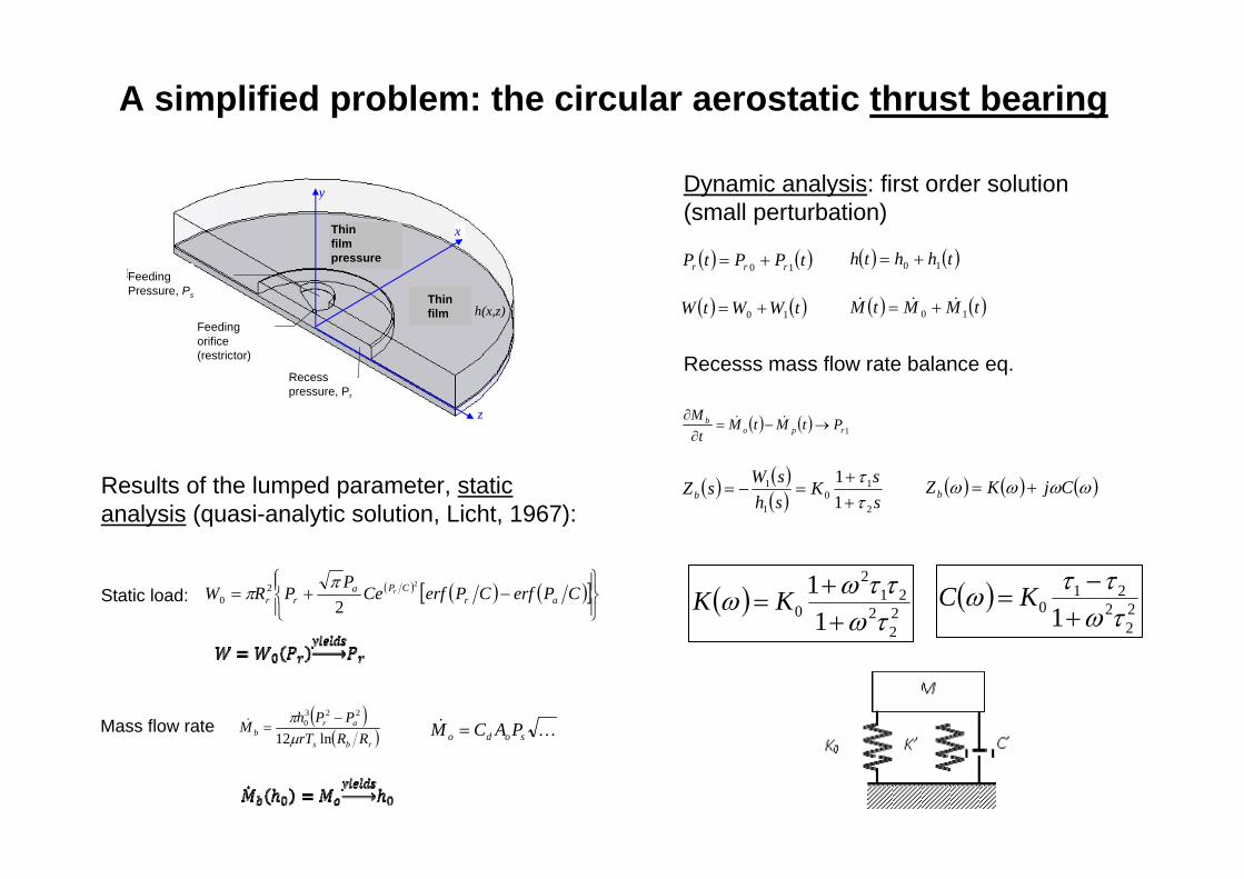
Results of the lumped parameter, staticanalysis (quasi-analytic solution, Licht, 1967):

A simplified problem: the circular aerostatic thrust bearing

CPerfCPerfCeP

PRW arCPa

rrr

2

22

0

Static load:

Mass flow rate rbs

arb RRrT

PPhMln12

2230

sodo PACM

Dynamic analysis: first order solution(small perturbation)

tPPtP rrr 10 thhth 10

tMMtM 10 tWWtW 10

Recesss mass flow rate balance eq.

1rpob PtMtM

tM

s

sKshsWsZb

2

10

1

1

11

CjKZb

22

221

2

0 11

KK 22

221

0 1

KC

x

Film mince d’épaisseur h(x,z)

Alvéole (poche) de pression Pr

Orifice d’alimentation (restricteur)

Pression dans le film mince P(x,z)

Pression d’alimentation Ps

z

y

Thinfilm

Thinfilmpressure

FeedingPressure, Ps

Feedingorifice(restrictor)

Recesspressure, Pr

0.2 0.3 0.4 0.5 0.6 0.7 0.8 0.9recess pressure/ supply pressure

0

100

200

300

400

500

600

700

800

900

1000

rece

ss d

epth

(µm

)

Damping (Ns/m)

Static stiffness Damping iso-lines for ω→0 (i.e. mass→ ∞)

Negative damping and the accompanying « pneumatic hammer » instability are controlled by:-Recess depth-The ratio Precess/Psupply

Characteristics of the aerostatic thrust bearing

Fuller (1984, pg. 534) suggests operating at high Precess/Psupply by usinglarge size orifice restrictors

Zone of pneumatichammer instability

Theoretical analysis: -1st step: steady CFD analysis-2nd step: « bulk flow » calculations of K and C (M→∞)

Theoretical investigation of the « pneumatic hammer »instability in the aerostatic bearing-Centered bearing-Zero rotation speed-Different diameters of the restrictor orifice: 50%, 68%, 84% and 100% of Dorifice

2nd step: «bulk flow» calculations of dynamic coefficients

Direct stiffness, K [N/m] Direct damping, C [Ns/m]

• Centered bearing and zero rotation speed• Mass →∞ i.e. (almost) zero excitation frequency

Zone of pneumatichammer instability

Experimental analysis of a single aerostatic bearing:the « floating bearing » test rig

ShakerMisalignementstinger

Dynamometer(static load)

Spindle

Hydrostaticdouble Lomakinbearing

Aerostatichybridbearing

A new aerostatic bearing with dismounting orifices of different diameters was designedand manufactured.

Experimental dynamic coefficients-Centered bearing-Zero rotation speed-Excitations applied by a single shaker in the range 250…450 Hz-Results obtained with three diameters of the restrictor orifice:

68%, 84% and 100% of Dorifice

Direct stiffness, K [N/m] Direct damping, C [Ns/m]

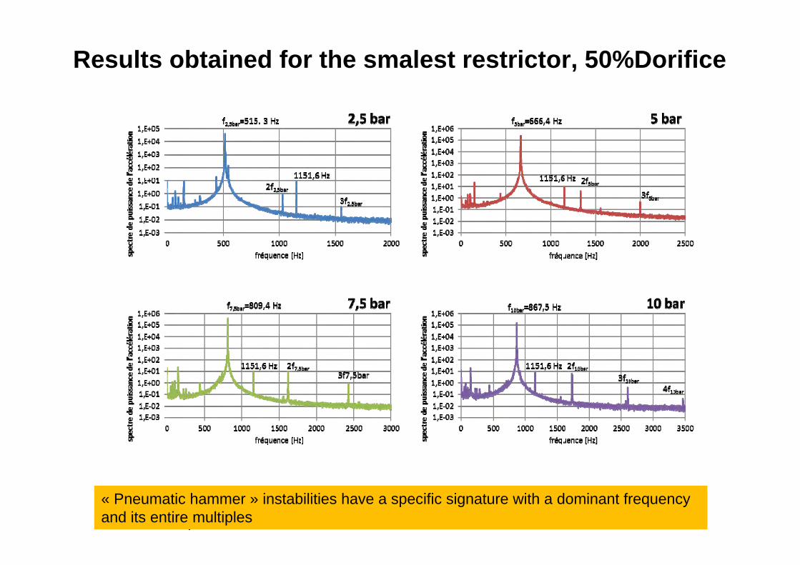
Results obtained for the smalest restrictor, 50%Dorifice

« Pneumatic hammer » instabilities have a specific signature with a dominant frequencyand its entire multiples

CONCLUSIONS

Acknowledgements

SNECMA Space Propulsion Division, Centre National d’Etudes Spatiales

Laurent RUDLOFF, Amine HASSINI, Franck BALDUCCHI, Lassad AMAMI, Sylvain GAUDILLERE

Is the work on hybrid aerostatic bearing finished?

- The accuracy of the predictions is satisfactory but can be still criticized; not allconfigurations are yet tested.

Will the hybrid hydro/aerostatic bearing finally replace ball bearings?

- Theoretical predictions are not very time consuming and enable parametric studiesbut very extensive theoretical analyses are still a problem (for example analyzing theimpact of manufacturing tolerances)

- The experimental activity is still going on and is continuously consolidated.

Thank you for your attention