theoretical analysis of the static deflection of plates ... · theoretical analysis of the static...

Theoretical analysis of the static deflection of plates for atomic force microscope applications

John Elie Sader and Lee White Department of Mathematics, University of Melbourne, Parkville, 3052 Victoria, Australia

(Received 25 January 1993; accepted for publication 8 March 1993)

The analysis of the static deflection of cantilever plates is of fundamental importance in application to the atomic force microscope (AFM). In this paper we present a detailed theoretical study of the deflection of such cantilevers. This~ shall incorporate the presentation of approximate analytical methods applicable in the analysis of arbitrary cantilevers, and a discussion of their limitations and accuracies. Furthermore, we present results of a detailed finite element analysis for a current AFM cantilever, which will be of value to the users of the AFM.

I. INTRODUCTION

The analysis of the static deflection of plates has been an area of considerable research activity, with many varying methods being developed for the analysis of plates of a specific shape and structure.lF5 In the case of a plate of arbitrary shape, however, the solution of the governing plate equation is a nontrivial matter and in general an exact analytical solution does not exist, thus necessitating the implementation of numerical methods.6 However, there do exist specific cases for which analytical procedures such as Fourier analysis may be applied4*5 in the solution of the plate equation.

In this paper, we shall consider the analysis of the static deflection of a cantilever type plate, i.e., a plate in which one edge is clamped and all other edges are free, as the knowledge of the static deflection of such plates is of fundamental practical importance in application to the atomic force microscope (AFM). We must at this stage emphasize that all previous analyses presented in Refs. 1-5, which give an exact analytical solution to the plate equation, are not applicable to plates of the form under consideration in this paper. Reissner et aL’ presented an approximate method for the evaluation of the static deflection of such plates. However, in Ref. 7 the authors com- ment that the resulting solution is in error by a factor of as much as ( 1 - 4) (where Y is Poisson’s ratio) as a result of the artificial restraint against anticlastic curvature. How- ever, as we shall show in the case of a symmetric plate with a symmetric load, this is in fact not the case, and only appears as a result of inconsistencies in the theory presented in Ref. 7 in the analysis of the lowest order term. To correct this error factor, it was proposed in Ref. 7 to implement a higher order analysis. We shall also show that there is no real advantage in going to such a higher order analysis, as this unduly complicates the analysis with no great increase in accuracy. Furthermore, in Ref. 7 the authors state that their method is applicable to plates of arbitrary shape and aspect ratio. However as we shall discuss and demonstrate, there is a limitation to the shape and aspect ratio of the plates, which comes about from the variation of the magnitude of the anticlastic curvature.

Apart from presenting an approximate theoretical treatment of an arbitrary cantilever plate, we shall also

evaluate and critically assess an approximate formula for the deflection of a cantilever plate currently in use in the AFM, as presented in Ref. 8. We shall show, by example and discussion, the invalidity of this formula.

We shall present the results of a detailed numerical analysis of the static deflection of the above mentioned cantilever,’ which to our knowledge has not hitherto ap- peared in literature, which will be of considerable practical value in the implementation of the AFM.

Finally, in the appendices we shall present a table of approximate spring constants obtained by the approximate theory for a number of different cantilevers. Also, we shall present a simple exact analytical expression for the average deflection of a rectangular cantilever, which may be used to quantify the accuracy of approximate analytical or purely numerical methods.

II. BACKGROUND THEORY

We shall begin by briefly summarizing the fundamental relationships and laws governing the deflection of plates, which shall be used throughout this paper. Note that the theory to be presented is only applicable to thin plates exhibiting small deflections.‘” In particular, we shall only be considering symmetric cantilever plates with symmetric loads, of which one such example is presented in Fig. 1, i.e., plates in which one edge is clamped and all other edges are free.

It is well known that the strains in an arbitrary thin plate are defined:’

a2w E,=--z,,z, (la>

ey=zg, (lb)

a% E"y=-baXay> (lc)

where w is the deflection function of the plate in the z direction. Furthermore, Hookes Law states

1 Ex’-jj (a,--y), (24

1 J. Appl. Phys. 74 (l), 1 July 1993 0021-8979/93/74(1)/l /g/$6.00 @ 1993 American Institute of Physics 1

Downloaded 30 Mar 2005 to 128.250.49.72. Redistribution subject to AIP license or copyright, see http://jap.aip.org/jap/copyright.jsp

FIG. 1. Figure of arbitrary symmetric cantilever plate showing point load F, and dimensions. 0 represents the origin of the coordinate system.

II=;J-J $$,+$+2(l-v)[~$

-(gJ2]]dXdY-JJWdXdY

- Q,,w ds, s

(4)

where D=E?/[12( 1 --?)I. Note that all integrals in Eq. (4) are taken over the cross-sectional area of the plate, except for the third integral where s is taken along the boundary of the plate and n is the corresponding outward normal to the boundary.

Following the above mentioned procedure, it can be easily shown2 that the well known plate equation results

Xl+v) exy=- r

E V’

where eX , ev, and eV are the x, y, and xy components of the strain tensor, respectively, whereas a,, a,, , and rXv are the x, y, and xy components of the stress tensor, respectively, and E is Young’s modulus. Finally, the x, y, and xy components of the bending moments per unit length are, respectively, defined as

My= I it -ft

zcry dz,

Mxy= ;t

s ‘t zrxv dz,

-5

(3b)

(3c)

where the integration is over the thickness t of the plate. It must be emphasized that Eqs. (la)-(3c) are only

applicable to thin plates. These nine equations will form the basis of all derivations and analyses to be presented in this paper.

In the pursuing section we shall present an approximate theory for the analysis of these cantilever plates.

111. APPROXIMATE THEORY

A. General plate equation

It is well known2 that the equation governing the deflection function w(x,y) of an arbitrary plate may be obtained directly from the minimization of its potential energy, by the implementation of a calculus of variations.’ As was shown in Refs. 1 and 2, the potential energy II of an arbitrary plate with only an external transverse load per unit area q(x,y) and a transverse shearing force per unit length Q, applied to its boundary is delined:

with boundary conditions as presented in Ref. 2. These boundary conditions shall not be reproduced, as they are complex in nature and are of no real value in this paper.

In. the case of an arbitrary plate, an exact analytical solution to Eq. (5) is extremely difficult if not impossible to obtain. Thus if an analytical solution to the static deflection of such plates is required, Eq. (5) is of no real value. To overcome this problem, it becomes necessary to implement some initial approximations and assumptions which greatly simplify the equation governing the de&c- tion.

The following derivation follows the same basic ideol- ogy as that presented in Ref. 7. However, instead of ini- tially considering the general form of the potential energy given in Eq. (4) and thus formulating the governing equations, as was performed in Ref. 7, we shall begin with the fundamental governing equations (la)-(3c). This procedure is essential, since beginning with Eq. (4) directly will result in a solution to the static deflection problem which is physically inconsistent and contradictory, as we shall discuss in detail. Note that this is the source of the resulting error in Ref. 7, in which the final solution is in error by a factor of as much as ( 1 - 2); as we shall also discuss in detail.

B. Zeroth order equations

In formulating the zeroth order solution, we search for an approximation to the true deflection function of the form

W(X,Y) -wobd, (6)

i.e., the true deflection function w, which is a function of x and y, is approximated by a function purely in x. Clearly, Eq. (6) would be expected to be a good approximation if there is little y variation in the deflection. One such case in which Eq. (6) is expected to be valid, is that of a narrow plate whose width is far smaller in magnitude than its length.

2 J. Appl. Phys., Vol. 74, No. 1, 1 July 1993 J. E. Sader and L. White 2


Clearly, if the zeroth order approximation to the true deflection function w(xy) made in Eq. (6) is to be physically consistent, then the following zeroth order approximation to the bending moments in they direction MY must also be made:

My-O, (7)

i.e., the approximation that all bending moments in the y direction be equated to zero. Note that this is essential, since any bending moment in the y direction will induce a y variation in the deflection, which clearly would be inconsistent and contradictory to Rq. (6). Thus, we can con- clude that Eqs. (6) and (7) are equivalent zeroth order approximations.

Furthermore, it is clear upon examination of the definition of MY in Eq. (3b), that Eq. (7) is equivalent and identical to the zeroth order approximation

au- 0, (8)

i.e., all stresses in they direction be approximated to zero. Therefore, it is clear from the above discussion that the

zeroth order approximation given in Eq. (6) is equivalent and simultaneously identical to the zeroth order approximations given in Rqs. (7) and (8). It must be emphasized that if any one of these approximations are made, then the others must also be simultaneously implemented if the approximation is to be physically consistent and valid.

Note that only the approximation presented in Rq. (6) was implemented in Ref. 7, with the complete neglect of Eqs. (7) and (8), which thus resulted in a solution which was physically inconsistent and furthermore in error by a factor of as much as ( 1 -g>, as we previously stated.

We shall now present the formal derivation qf the governing equations for the zeroth order approximation to the deflection function given in Eq. (6).

Substitution of Eqs. (6)-( 8) into the governing stress- strain relations given in Rqs. (la)-(2~) results in

d2w,. %=-zyg-’

Ey’Exy’O, (9b)

oX=EeX, (104

ay=rxy=o, (lob)

and from Eqs. (9a>-( lob), it can be easily shown that

d2wo 1MX=---D’~’ (114

where

Et3 D’=z. (llc)

Thus from Eqs. (9a)-( 1 lc), it can be shown in an identical manner to Ref. 2 that the strain energy VapProX of an arbitrary plate under these approximations is defined by

v,prox=; j-j-D’ (2) ‘d, dy. (12)

Finally for a plate with an external transverse load per unit area q(x,y) and transverse boundary edge forces per unit length Q,, the resulting expression for the potential energy II approx of the plate under the approximations of Eqs. (6)- (8) is defined:

- s

Q,,wo ds. (13)

Again note, that if the approximation presented in Eq. (6) were substituted directly into the original expression for the potential energy of a plate under no initial assumptions, as presented in Eq. (4), a result would be obtained which would be physically inconsistent and contradictory, and would ‘be in error by a factor of as much as ( 1 -?>, as is clearly evident upon comparison of Eqs. (4) and ( 13 ) .

Referring to Fig. 1 and Rq. ( 13), it is clear that all integrals with respect to y may be removed to obtain

~~~~~~~~~ s,” 4x1 ( s)2dx- s,” h(x)wo dx

-fio(L)t (14)

where

s

f(x) a(x) = D’ dy, (154

-f(x)

f(x) h(x) =

s dw)d., (15b)

-f(x)

(15c)

Note that in the formulation of Eqs. (14)-( 15c), only boundary edge forces at the end. tip of the plate have been considered, since this is all that is required for AFM applications.’

Then upon implementation of the calculus of varia- tionsg to Rq. (14) with respect to wO(x), it can be easily shown that the governing equation for w,-Jx) is defined as

-$2 (a(x) $)=h(x) with boundary conditions

dwo web) =--& 1 =o, x=0

(16)

(174

(17b)

(17c)

3 3 J. Appl. Phys., Vol. 74, No. 1, 1 July 1993 J. E. Sader and L. White


It must be noted that in general an exact analytical solution to Eqs. (16)-( 17~) is possible, thus eliminating the otherwise necessity for the implementation of numerical methods, as is the case with the original plate equation (5).

At this stage it must be noted that Eq. (6) is in fact only the first term in an infinite power series expansion for the true deflection function7

d&Y) = i; W2nWy2n. (18)

Only even terms have been considered in Eq. ( 18), since in this paper we are only considering symmetric plates with symmetric loads.

Reissner et al7 stated that the results for the static deflection would be in error by a factor of as much as (1 -g), and as we have just shown this is not the case. Furthermore, to correct this and to obtain greater accuracy, the authors suggested that higher order terms in Eq. (18) be implemented in the analysis.

C. Second order equations

The approximation suggested in Ref. 7, has the form

W(X,Y) -we(x) +JJwz(x>

which is the first two terms in Eq. ( 18). (19)

Note that in this case, nothing can be deduced about the bending moments and stresses as was the case in the preceding section, and therefore, the approximation in Eq. ( 19) stands alone and may be substituted directly into the general expression for the potential energy of the plate, as given in Eq. (4). Since the full implementation of Eq. ( 19) was not carried out in Ref. 7, we shall present the governing second order equations, suppressing all derivations since they are performed in an analogous manner to that in the preceding section and Ref. 7.

Thus, it can be easily shown that the governing second order equations for the functions we(x) and w2(x) are defined as

-$ (a,(x) ($?,2-) +A&) z]--8(1---y) $

d2w2 +2~4(x) z=Zs(x)

with boundary conditions

(214

(21b)

dwo dw w&x) =-&=w2w =J-p x=o=o’ 1

[4(x) ($+2-j +&Ax> gq=,=o, (2ld)

(%[a,~x~(~+2~w2)+a,cx,~]-8~l--Y)

x [a,(x) $t] 1,=,=Q WeI

where

s

f(x) Ai = Dy’-’ dy,

-f(x) (224

s

f(x) Z,(x) = -n ) q(x,y)y’-’ dy, Wb)

x p= f(L) s Qn dy7 (22cj

-f(L)

where i is an integer. Note that as in Eqs. (14)-( 15c), only boundary edge

forces at the end tip of the plate have been considered in the formulation of Eqs. (20a)-(22c).

The increased complexity of the second order equations in comparison with the zeroth order equations is clearly obvious upon comparison of Eqs. ( 16)-( 17~) with Eqs. (20a)-(22c). Furthermore, unlike the zeroth order equations, an analytical solution to the second order equations is not obvious, if at all possible in even the most trivial case, and thus numerical methods must be resorted to. However, it must still be noted that Eqs. (20a)-(22c) are far simpler to analyze than the original plate equation (5). In the pursuing sections we shall examine the accuracy and applicability of the second order equations in comparison with that of the zeroth order method and a complete numerical treatment of the plate equation (5).

Before we present the comparison, it must be noted that the second order solution only contains the first two terms in an intinite power series of the true deflection function w (x,y), thus it is also expected to be only applicable to plates where the anticlastic curvature is relatively small. This shall also be examined in the pursuing sections.

IV. DlSCUSSlON

We shall now critically assess the applicability and accuracy of the zeroth order and second order solutions by a comparison with a direct numerical treatment of the original governing plate equation (5). In particular, a finite element analysis6 of Eq. (5) has been implemented.

It must be noted that in application to the AFM, the coefficient of prime importance is the “spring constant” which is defined to be the force required per unit deflection at the end tip of the plate. In this paper, we shall be con-



1.25 1.5 1.75 2

c

FIG. 2. Plot of K-rel=kFE/kapprOn where “FE” and “approx” refer to results obtained by the kite element and approximate method respectively, for (a) v=O, (b) v=O.25, and (c) v=O.4. Zeroth order solution (solid line). Second order solution (dashed line).

sidering a point force appl ied to the end tip, and its corresponding deflection, as shown in F ig. 1. Hence, the spring constant is formally def ined as

(23)

where F is the magn itude of the appl ied force, and (xofio) is its corresponding position of application.

F irst of all, the case of a rectangular plate shall be considered, as shown in F ig. 1, with f(x) =c/2 and L= 1. A comparison of the spring constants obtained by the zeroth order and second order methods with respect to a direct finite element solution of Eq. (5) for varying plate parameters is given in F igs. 2(a)-2(c). The zeroth order solution is given in Appendix A, whereas the results for the second order method were obtained by the implementation of a fourth order Runge-Kutta method for the solution of systems of first order ordinary differential equat ions” in conjunction with a shooting method for the solution of the two point boundary value problem,” as is clearly required upon examination of Rqs. (20a)-(22c).

It is clear from F igs. 2(a)-2(c), that the zeroth order and second order methods possess similar accuracies, with

the second order method possessing slightly better accuracy. Note that as the width of the plate is increased, it is also expected that the magn itude of the anticlastic curvature increase, and therefore a corresponding decrease in the accuracy of both the zeroth order and second order methods, and this is clearly borne out in F igs. 2(a)-2(c). It is also clear from the results that for a given accuracy, the second order method possesses a slightly larger range of applicability, as expected. However, the analysis of the second order equat ions is clearly far more complex than the zeroth order equations, since numerical methods must be resorted to for its solution in comparison to the zeroth order equat ions whose solution may be easily obtained by analytical means.

To make a further comparison, we shall now consider a plate in which the sides are adjustable to a gradient pa- rameter m, i.e., referring to F ig. 1, the dimensions of the plate are f(x) = 1 -mx. The results of a comparison of the zeroth order and second order solutions given in this paper, and the zeroth order solution given in Ref. 7 with respect to the finite element solution are given in Table I for the normalized deflection W at the end tip, where W = w2D’/F. It is again clear, that increasing the anticlastic curvature (in this case decreasing the length) decreases the accuracy of both the zeroth order and second order methods. Furthermore, as stated above, the second order method for a given accuracy has a slightly wider range of applicability, as is clear from Table I. Note that the results of the zeroth order analysis presented in Ref. 7 possess poorer accuracy than those of the zeroth order and second order solutions presented in this paper, as expected for reasons discussed in the preceding section. The results for the second order solution are slightly better than those for the zeroth order solution, however note that both zeroth and second order solutions are only applicable to plates in which the anticlastic curvature is relatively small.

Thus upon consideration of these results and the discussion presented in the preceding section, it must be con- c luded that there is no real advantage in the second order method over the zeroth order method, and in fact can be concluded as disadvantageous. The reasons being that the accuracies and ranges of applicability of both methods are similar, however the analysis of the second order method is far more complex than that of the relatively simple zeroth order equations, as discussed above.

Furthermore, it must be emphasized that the zeroth order and second order methods are only applicable to plates in which the anticlastic curvature exhibited in the deflection can be considered as relatively small, contradictory to the comments presented in Ref. 7 which imply that such zeroth order and second order methods are applicable to arbitrary thin plates.

V. AFM CANTILEVER

In this section a cantilever of fundamental practical importance in application to the AFM shall be considered, and results shall be presented for the spring constant for arbitrary dimensions of this cantilever. The general form of the cantilever currently in use* is that given in F ig. 3,



TABLE I. Table showing comparison of normalized deflection at point of application of load as shown in Fig. 1 for plate with f(x) = I- mx and (a) L=3, (b) L=2, and (c) L=l. “Zeroth”, “second”, “old”, and “FE” refer to results obtained by the zeroth order, second order, method presented in Ref. 7, and finite element method, respectively. Percentage errors with respect to the finite element results are indicated in parenthe- SeS.

W zemth W second weld WFE m Y Cm*) (m2) (m’) (ma)

(a) 0

0

0

0.133

0.133

0.133

0.267

0.267

0.267

(b) 0

0

0

0.2

0.2

0.2

0.4

0.4

0.4

(cl 0

0

0

0.4

0.4

0.4

0.8

0.8

0.8

0

0.25

0.4

0

0.25

0.4

0

0.25

0.4

0

0.25

0.4

0

0.25

0.4

0

0.25

0.4

0

0.25

0.4

0

0.25

0.4

0

0.25

0.4

9.000 (1.6) 9.000

(6.5) 10.08 (0.8) 10.08 (1.0) 10.08 (5.4) 11.83 (0.7) 11.83 (0.2) 11.83 (3.0)

2.667 W-0 2.667

(0.7) 2.667

(4.8) 2.987

(2.8) 2.987

(1.3) 2.987

(3.5) 3.506

(2.5) 3.506

(2.8) 3.506

WI

0.333 (17.0)

0.333 (16.8)

0.333 (i1.3)

0.373 (15.9)

0.373 (16.1)

0.373 (10.3)

0.438 (14.7)

0.438 (17.0)

0.438 (13.1)

9.033 (0.7)

8.738 (1.4) 8.230

(2.3) 10.12 (0.5) 9.899

(0.9) 9.432

(1.4) 11.89 (0.2) 11.81 (0.4) 11.42 (0.6)

2.699 (1.6) 2.613

(2.8) 2.442

(4.0) 3.029

(1.3) 2.972

(1.8) 2.813

(2.4) 3.573

(0.6) 3.574

(0.8) 3.445

(1.0)

0.359 (8.6) 0.354

(10.1) 0.332

(11.7) 0.411

(5.4) 0.411

(5.6) 0.390

(5.6) 0.496

(1.4) 0.506

(1.3) 0.489

(1.4)

9.000 (1.0) 8.438

(4.8) 7.560

(10.2) 10.08 (0.8) 9.452

(5.3) 8.469

(11.4) 11.83 (0.7) 11.09 (6.5) 9.939

(13.5)

2.667 (2.8) 2.500

(6.9) 2.240

(11.8) 2.987

(2.8) 2.801

(7.5) 2.509

(12.9) 3.506

(2.5) 3.287

(8.8) 2.945

(15.3)

0.333 (17.0)

0.313 (19.7)

0.280 (24.5)

0.373 (15.9)

0.350 (19.3)

0.314 (23.9)

0.438 (14.7)

0.411 (19.9)

0.368 (25.7)

9.093

8.860

8.418

10.17

9.985

9.562

11.92

11.86

11.49

2.742

2.687

2.540

3.070

3.027

2.882

3.595

3.603

3.478

0.390

0.389

0.371

0.433

0.434

0.412

0.503

0.513

0.496

Y-----7 t z

//$x52& 1--I’, (q2 LJ \\,lF / ‘)I/x.. ‘i

1’

FIG. 3. Current AFM cantilever model used in analysis showing point load F, and dimensions. 0 represents the origin of the coordinate system.

where a point load has been applied to the end tip. At first sight the analysis of this plate appears to be

relatively simple, if each arm of the plate is considered to be a rectangular plate and both plates are joined in parallel, as was proposed in Ref. 8. However, as we shall show, this approximation -(which shall henceforth be referred to as the “parallel plate approximation”) is physically dubious and numerically inaccurate under a wide range of cantilever geometries.

For such a plate whose arm width d is not far smaller in magnitude to the overall width b, great ambiguity arises in the determination of the length of each individual arm, and furthermore the plate cannot be considered as consist- ing of two rectangular plates in parallel. Second, for a plate in which d 4 6, ambiguity in the length still arises, although this is of course much smaller than in the previous case, however, for a plate where the aspect ratio (A=b/L)A > O( 1) , torsion of the arms becomes a significant factor, as we have found by conducting a rigorous finite element analysis of the original plate equation. ‘This leads to a deflection function which does not resemble that of two rectangular plates in parallel, and thus leads to great inaccuracies in the approximation. Finally, in the case where d Q b and A 4 O( 1)) torsion of the arms does not appear to be a problem, however, in this case ambiguity again arises in the length of each arm. The inaccuracies of this approximation shall be demonstrated shortly. A. Finite element results

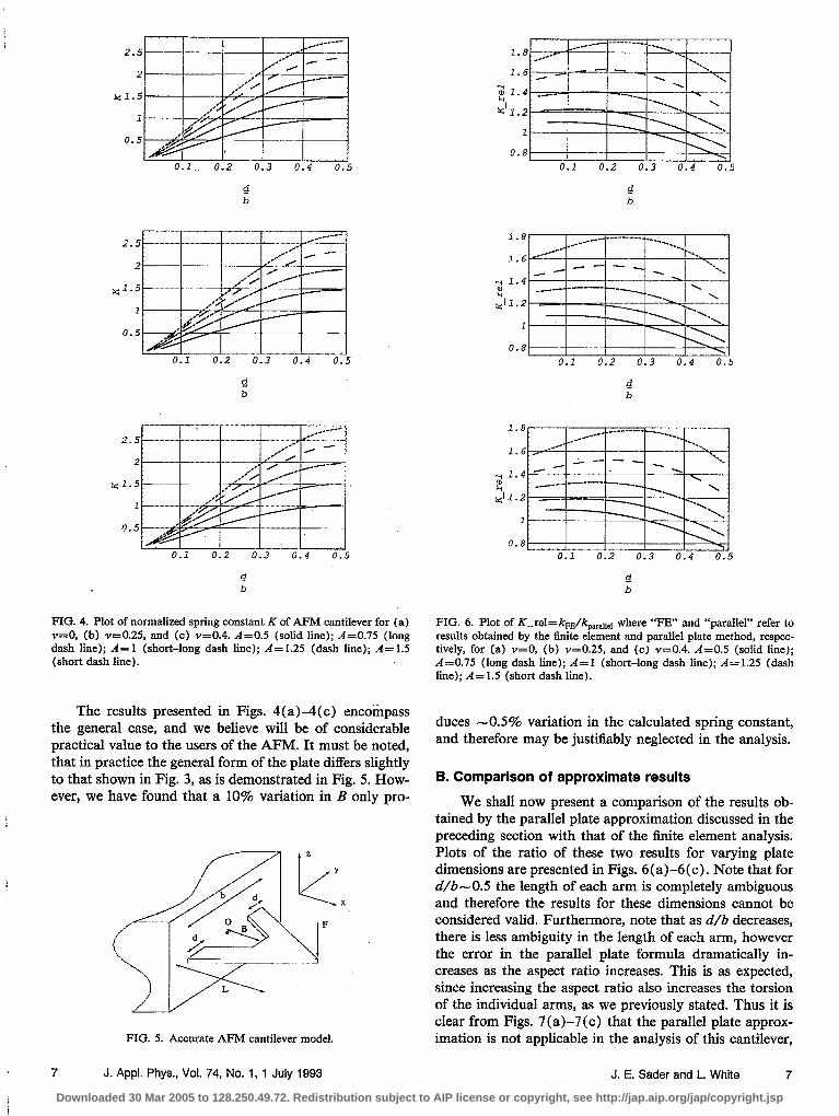
We have implemented a complete finite element analysis’ of the cantilever presented in Fig. 3, the results of which are presented in Figs. 4(a)+c) for various aspect ratio A, Poisson’s ratio V, and width ratio d/b. Note that these results are for a normalized spring constant K which is independent of Young’s modulus E and the thickness t of the plate. The actual spring constant k can be obtained simply and directly from the following definition:

KD’ k=F (N m-l),

where D’ is as defined in Eq. ( 1 lc) and L is the actual length of the cantilever, as illustrated in Fig. 3.



d 52 b b

2.5

2

xl.5

1

0.5

0.1 0.2 0.3 0.4 0.5

52 b

0.1 0.2 0.3 0.4 0.5

d d b b

FIG. 4. Plot of normalized spring constant K of AFM cantilever for (a) v=O, (b) v=O.25, and (c) v=O.4. ii=O.5 (solid line); A=0.75 (long dash line); I$=1 (short-long dash line); A=l.25 (dash line); A=1.5 (short dash line).

The results presented in Figs. 4(a)-4(c) encompass the general case, and we believe will be of considerable practical value to the users of the AFM. It must be noted, that in practice the general form of the plate differs slightly to that shown in Fig. 3, as is demonstrated in Fig. 5. How- ever, we have found that a 10% variation in 3 only pro-

FIG. 5. Accurate AFM cantilever model.

We shall now present a comparison of the results obtained by the parallel plate approximation discussed in the preceding section with that of the finite element analysis. Plots of the ratio of these two results for varying plate dimensions are presented in Figs. 6 (a)-6 (c) . Note that for d/b-O.5 the length of each arm is completely ambiguous and therefore the results for these dimensions cannot be considered valid. Furthermore, note that as d/b decreases, there is less ambiguity in the length of each arm, however the error in the parallel plate formula dramatically increases as the aspect ratio increases. This is as expected, since increasing the aspect ratio also increases the torsion of the individual arms, as we previously stated. Thus it is clear from Figs. 7(a)-7(c) that the parallel plate approximation is not applicable in the analysis of this cantilever,


x

1.8

1

0.8 0.1 0.2 0.3 0.4 0.5

1.8

0.8 0.1 0.2 0.3 0.4 0.5

d b

1.8

1.6

0.8 0.1 0.2 0.3 0.4 0.5

FIG. 6. Plot of K-rel=kFE/kparallcl where “FE” and “parallel” refer to results obtained by the finite element and parallel plate method, respac- tively, for (a) v=O, (b) v=O.25, and (c) v=O.4. A=0.5 (solid line); A=0.75 (long dash line); *4= 1 (short-long dash line); Azl.25 (dash line); A=1.5 (short dash line).

duces -0.5% variation in the calculated spring constant, and therefore may be justifiably neglected in the analysis.

B. Comparison of approximate results


52 b

0. 1 E %‘O.

0.

V.,d

0.9

z 0.85

&' 0.8

0.75

0.7

c! b

8

d b

FIG. 7. Plot of K-rel=kFE/kx,th where “FE” and “zeroth” refer to results obtained by the finite element and zeroth order method, respectively, for (a) v=O; (b) v=O.25, and (c) v=O.4. A=0.5 (solid line); .4=0.75 (long dash line); A= 1 (short-long dash line); A=1.25 (dash line); A= 1.5 (short dash line).

as has been suggested by Albrecht et al.’ As an example, for some typical values of a cantilever in current use, ~=0.25, A= 1, and d/b=0.2 (Ref. 12) the parallel plate approximation is in error by -25%.

In Figs. 7(a)-7(c) results are presented of a similar comparison for the zeroth order solution of this cantilever (presented in Appendix A). Note that for d/b-0.5, quite good accuracy is obtained by the zeroth order solution, with all errors 5 lo%, for the range of aspect ratio chosen. Note also that decreasing d/b increases the magnitude of the anticlastic curvature and therefore decreases the accuracy of the zeroth order solution, however this is as expected since the zeroth order solution is only formally valid for plates exhibiting a relatively small anticlastic curvature. Note that for the typical values used above, the zeroth order solution still produces a reasonably accurate result with error - 13% as compared with -25% for the parallel plate approximation. Thus depending on the application, one may choose to use the simple zeroth order approximation over the far more complicated direct numerical treatment of the original plate equation. +

8 J. Appl. Phys., Voi. 74, No. 1, 1 July 1993 J. E. Sader and L. White 8

VI. CONCLUSION

We have presented a detailed theoretical study of the static deflection of cantilever plates for AFM applications. This incorporated both an approximate analytical analysis and a rigorous finite element analysis of the original plate equation.

The approximate analysis presented is valid for an arbitrary cantilever plate which exhibits relatively small anticlastic curvature, and we have shown that even for plates where the anticlastic curvature is not small, the zeroth order approximation still gives reasonably accurate results ( - 13% error). Furthermore, we have shown that the zeroth order solution is not in error by a factor of as much as (l-2) due to the artificial restraint against anticlastic curvature, and that there is no real advantage in pursuing a second order analysis over the zeroth order analysis, as were both suggested by Reissner et a1.7

For the current AFM cantilever, as shown in Figs. 3 and 5 and Ref. 8, we presented a critical assessment of the parallel plate approximation suggested in Ref. 8 for the evaluation of the spring constant, and discussed and demonstrated its inaccuracy and invalidity. Furthermore, we presented the results of a rigorous finite element analysis of this cantilever, which we believe will be of great practical value to the users of the AFM.

ACKNOWLEDGMENTS

The authors would like to express their gratitude to Dr. J. F. Williams of the Department of Mechanical En- gineering for many interesting and stimulating discussions, and for providing access to the finite element package used in this paper. This research was funded by the Advanced Minerals Products Center, an ARC special research center.

APPENDIX A

In this Appendix the explicit expressions for the spring constants k of some specific cantilever plates obtained by the zeroth order method are presented. The results presented here are in reference to Fig. 1. ( 1) Rectangular plate:

f (xl ==Yl, (Ala)

6D’Yl k=T. (Alb)

(2) Triangular plate:

f(x) =+ (L--x),

41)‘; k=L3.

(A24

(A2b

(3) Trapezoidal plate: f(x)=a(l-mx),

2 D’am3 m2L2 k=-

mL--l mL-2(l-mL)

1-l

(A3a

+(1-mL)ln(l-mL) . I

Mb)


(4) Truncated parabolic plate:

f(x)=a[ l-m(:)‘], (A4aj

k=2D’a 5 l+m -1

-1+- 6 tanh-.‘( fi)+ln(l-m) . 1 (A4b) (5) AFM cantilever (see Fig. 3):

6 D’b3d k=

m* (A51

APPENDIX B

In this Appendix we present the formal derivation of the exact average deflection function for a rectangular cantilever with Y=O, i.e., f(x) =yl in Fig. 1.

Beginning with the plate equation (5) and expanding, we rind

a4W a‘b a5l.J q(x,y)

=+2ax’a3#+v= D * (Bl)

The following definition is then made for the average deflection function zZ( x) :

1 Yl C(x) =-

s 2Yl -y* w(x,yMy, 032)

where 2yr is the width of the plate. Upon integration of Eq. (Bl ) with respect to y over

the cross section of the plate, it can easily be shown that the following equation results:

(B3)

where

Q(x) =& ry, q(w)&. V34)

However, from the boundary conditions2 for Eq. (5)) we have the following condition along the edges y= ~yt :

a3W a3w -&T+ (2---y) p&=0. U35)

Thus, substituting Eq. (BS) into Eq. (B3), the following equation results for Y=O, and for a point load on the end of magnitude F [i.e., q(x,y) =FS(x--L)S(y)], as shown in Fig. 1,

a% FS(x--35) dxa’ 2ylD 036)

with boundary conditions

0374

=o, x=L

(B7b)

(B7c)

The solution of which follows directly and is given by

W(x) = -- ,;;L1 (x--3L) CBS)

which can be shown to be identical to the zeroth order solution.

’ E. H. Mansfield, The Bending and Stretching of Plates (Pergamon, Oxford, 1964).

2S. Tiioshenko and S. Woinowsky-Krieger, Theory of PIates and Shells (McGraw-Hill, New York, 1959).

‘L. D. Landau and E. M. Lifshitz, Theoty of Elasticity (Pergamon, Oxford, 1970).

4M. Levy, C. R. Acad. Sci. 129, 535 (1899). ‘T. J. Jaramillo, J. Appl. Mechan. 17, 67 (1950). ‘PAFEC is a trademark of, and is available from PAFEC Ltd, Strelley

Hall, Main Street, Strelley, Nottingham, NG8 6PE. ‘E. Reissner and M. Stein, N.A.C.A. Tech. Note. No. 2369 (June 1951). ‘T. R. Albrecht, S. Akamine, T. E. Carver, and C. F. Quate, J. Vat. Sci. Technol. A 8, 3386 (1990).

‘V. I. Smirnov, A Course of Higher Mathematics (Pergamon, Oxford, 1964), Vol. 4.

‘OR. W. Hornbeck, Numerical Methods (Quantum, New York, 1975). “S. M. Roberts and J. S. Shipman, Two-Point Boundary Value Problems:

Shooting Methods (Elsevier, New York, 1972). “C. Drummond (personal communication).



theoretical analysis of the static deflection of plates ... · theoretical analysis of the static...

Documents