Theme IV – Understanding Seismicity

Catalogs and Their Problems

Catalog artifacts and quality control

L. Gulia1 • S. Wiemer2 • M. Wyss3

1. Istituto Nazionale di Geofisica e Vulcanologia, Italy 2. Swiss Seismological Service, ETH Zurich 3. World Agency Planetary Monitoring & Earthquake Risk, Geneva, Switzerland

How to cite this article:

Gulia L., S. Wiemer, and M. Wyss (2012), Catalog artifacts and quality controls,

Community Online Resource for Statistical Seismicity Analysis,

doi:10.5078/corssa-93722864. Available at http://www.corssa.org.

Document Information:

Issue date: 2 February 2012 Version: 1.0

2 www.corssa.org

Contents 1 Motivation ................................................................................................................................................. 4

2 Starting Point............................................................................................................................................ 4

3 Ending Point ............................................................................................................................................. 4

4 Theory ....................................................................................................................................................... 5

5 Examples of Excellent Applications in the Literature .............................................................................. 16

6 Links to Software and Catalogs ................................................................................................................ 24

7 Summary .................................................................................................................................................. 24

Catalog Artifact and Quality Control 3

Abstract Man-made contaminations and heterogeneity of reporting are present in all earthquake catalogs. Often they are quite strong and introduce errors in statistical analyses of the seismicity. We discuss three types of artifacts in this chapter: The presence of reported events, which are not earthquakes, but explosions; heterogeneity of resolution of small events as a function of space and time; and inadvertent changes of the magnitude scale. These problems must be identified, mapped, and excluded from the catalog before any meaningful statistical analysis can be performed. Explosions can be identified by comparing the rate of day-time to night-time events because quarries and road construction operate only during the day and often at specific hours. Spatial heterogeneity of reporting small events comes about because many stations record small earthquakes that occur near the center of a seismograph network, but only relatively large ones can be located outside the network, for example offshore. To deal with this problem, the minimum magnitude of complete reporting, Mc, has to be mapped. Based on the map of Mc, one needs to define the area and the corresponding Mc, the choice of which leads to a homogeneous catalog. There are two approaches to the strategy for selecting an Mc and its corresponding area of validity: If one wishes to work with the maximum number of earthquake per area for statistical power of resolution, one needs to eliminate from consideration areas of inferior reporting and use a small Mc(inside), appropriate for the inside of a network. However, if one wishes to include areas outside of the network, such as offshore areas, then one has to cull the catalog by deleting all small events from the core of the network and accept only earthquakes with magnitude larger than Mc(outside). In this case, one pays with loss of statistical power for the advantage of covering a larger area.

As a function of time, changes in hardware, software, and reporting procedure bring about two types of changes in the catalog. (1) As a function of time the reporting of small earthquakes improves because seismograph stations are added or detection procedures are improved. (2) The magnitude scale is inadvertently changed due to changes in hardware, software, or analysis routine. The first problem is dealt with by calculating the mean Mc as a function of time in the area chosen for analysis. This will usually identify steps of Mc downward (better resolution with time) at fairly discrete times. Once these steps are identified, one is faced with choosing a homogeneous catalog that covers a long period, but with a relatively large Mc(long time). This way one gains coverage of time, but pays with loss of statistical power because small events, which are completely reported during recent times, have to be eliminated. On the other hand, if one wishes to work with a small Mc(recent), then one must exclude the older parts of the catalog in which Mc(old) is high.

To define the magnitude scale in a local or regional area in such a way that it corresponds to an international standard is not trivial, nor is it trivial to keep the scale constant as a function of time, when hardware, software, and reporting procedures keep changing. Resulting changes are more prominent in societies characterized by high intellectual mobility, and may not be found in totalitarian societies, where observatory procedures are adhered to with military precision.

4 www.corssa.org

There are two types of changes: simple magnitude shifts and stretches (or compressions) of the scale. Here, we show how to identify changes of the magnitude scale and how to correct for them, such that the catalog approaches better homogeneity, a necessity for statistical analysis.

1 Motivation

Results obtained using a contaminated dataset have no statistical significance and may be misleading. For this reason, a careful identification of man-made changes should represent the first step in any statistical analysis of seismicity; their removal the second. Most such changes manifest themselves as changes in seismicity pattern and generate variations in the observed seismicity rates by up to 40% (Habermann 1986; Tormann et al. 2010). Such artificial patterns could be mistaken for possible precursors of large earthquakes (e.g. Wyss et al. 1981, 1983, 1984) or for periods of increased seismicity (Habermann 1986). Additional examples are the presence of non-tectonic events that may mask periods of seismic quiescence in a region, interferes with the investigation of active faults or yields a wrong frequency-magnitude distribution (e.g. high or low b-values).

2 Starting Point

In order to test the removal of non-tectonic events and the detection of changes in magnitude, access to an earthquake catalog is required. The earthquake regional catalogs used in this chapter are:

CSI 1.1 (Italian Earthquake Catalog, 1981-2002);

ROMPLUS (Romanian Earthquake Catalog, 1980-2006);

ReNaSS (French Earthquake Catalog, 1980-2005); Such catalogs are here provided both in ASCII and Matlab format (see repository materials), according to the software ZMAP (Wiemer 2001). They are composed by the following 8 columns

Longitude Latitude Year Month Day Magnitude Depth Hour Min

ZMAP is a Matlab-based open-source code, a set of tools designed to help seismologist analyze catalog data and also useful in routine network operations. Recently the beta version of the MapSeis software has been released and contains the ZMAP tools: the final version of MapSeis will have same functionality as ZMAP and will fully replace it. Both beta version of MapSeis and ZMAP are freely downloadable via the software section of the CORSSA website.

3 Ending Point

The aim of this article is to underline the presence of artifacts that should be removed before any statistical analysis. Tools to detect and remove artifacts, as

Catalog Artifact and Quality Control 5

well as their limitations, are also explained. By the end of this article, the reader should be able to identify and remove man-made contaminations from a catalog.

4 Theory

4.1 General processing

Here we describe the preliminary general processing of a catalog that should be performed before any statistical analysis of the seismicity. The aim of such processing is the identification and, if possible, removal of man-made contaminations. This processing is composed of:

1. Removal of non-tectonic events (i.e. explosions and quarry blasts) from the dataset;

2. Analysis of the homogeneity of reporting as a function of time and magnitude.

4.2 Explosions

Some instrumental seismicity catalogs describe the type of event among the optional parameters (e.g., tectonic event, explosion, quarry blast, induced event; see

Woessner et al. 2011). But often, despite network operators’ best efforts to identify blasts, such events are erroneously included in the catalogs. These events have low magnitudes and produce an enrichment in the number of small earthquakes: such an increase of microseismicity may be misinterpreted as a change in the natural phenomena. Recently Horasan et al. (2009) found that 85% of the investigated

seismic events near Istanbul (179 with 1.8≤Md≤3.0; KOERI-NEMC digital database) were quarry blasts. Wiemer and Baer (2000) presented an example of quarry blast contamination in the catalogs of Alaska, Switzerland and the Western United States while a detection of artificial events in European regional catalogs has been performed by Gulia (2010). Different methods have been designed to discriminate natural events from artificial ones (e.g., Bath 1975; Murphy and Bennet 1982; Kafka 1990; Wuester 1993; Musil and Plesinger 1996; Koch and Faeh 2002; Parolai et al. 2002), but these techniques require inspection of the seismograms of all events and the results obtained by different authors usually indicate that identification success varies strongly from station to station. After a the catalog is released, seismologists use them without further analysis of possible artificially introduced rate changes, assuming explosions have been eliminated and reporting procedures have been uniform as a function of space and time.

6 www.corssa.org

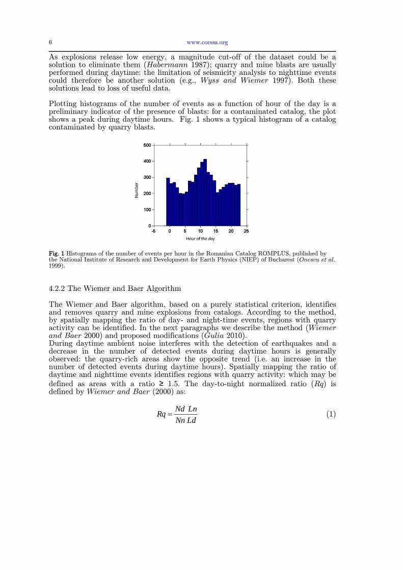
As explosions release low energy, a magnitude cut-off of the dataset could be a solution to eliminate them (Habermann 1987); quarry and mine blasts are usually performed during daytime: the limitation of seismicity analysis to nighttime events could therefore be another solution (e.g., Wyss and Wiemer 1997). Both these solutions lead to loss of useful data. Plotting histograms of the number of events as a function of hour of the day is a preliminary indicator of the presence of blasts: for a contaminated catalog, the plot shows a peak during daytime hours. Fig. 1 shows a typical histogram of a catalog contaminated by quarry blasts.

Fig. 1 Histograms of the number of events per hour in the Romanian Catalog ROMPLUS, published by the National Institute of Research and Development for Earth Physics (NIEP) of Bucharest (Onescu et al. 1999).

4.2.2 The Wiemer and Baer Algorithm

The Wiemer and Baer algorithm, based on a purely statistical criterion, identifies and removes quarry and mine explosions from catalogs. According to the method, by spatially mapping the ratio of day- and night-time events, regions with quarry activity can be identified. In the next paragraphs we describe the method (Wiemer and Baer 2000) and proposed modifications (Gulia 2010). During daytime ambient noise interferes with the detection of earthquakes and a decrease in the number of detected events during daytime hours is generally observed: the quarry-rich areas show the opposite trend (i.e. an increase in the number of detected events during daytime hours). Spatially mapping the ratio of daytime and nighttime events identifies regions with quarry activity: which may be

defined as areas with a ratio ≥ 1.5. The day-to-night normalized ratio (Rq) is defined by Wiemer and Baer (2000) as:

LdNn

LnNdRq (1)

Catalog Artifact and Quality Control 7

where Nd is the total number of events in the daytime, Nn in the night-time period, Ld is the number of hours in the daytime period and Ln in the night-time period (Ln + Ld = 24). The ratio is calculated using a regularly spaced grid covering the area studied and sampling only the N (N = Nd + Nn) closest epicenters to each node (Wiemer and Wyss 1994, 1997). The sample size, N, is a free parameter of the mapping: the code performs a grid search over the N parameter space (Nmin = 50, Nmax = 400, Nstep = 50) to identify the sample size with the highest Rq. Therefore, the parameter space spans three dimensions: latitude, longitude and sample size N. Once Rq has been computed for this three-dimensional grid, the node with the most anomalous Rq is identified: Rq is translated into a probability of occurrence, using a numerical simulation. 106 randomly distributed sample datasets are constructed, each containing N numbers in the time interval 0.00 - 23.59 h. Finally the code computes Rq for each hourly bin and each Rq is translated into a probability of occurrence. A value PRq(N) = 99% indicates that the probability to observe such a Rq(N) value by chance is 1% or less. The sample near a node with Rq(x,y,N) will be removed from the dataset if it exceeds the 99% threshold. The process is iterative: it is repeated until no volumes with an anomalous ratio of daytime to nighttime events with significance greater than 99% remains. A test for aftershock sequences is also performed, because a mainshock with its largest portion of aftershocks during the daytime hours of the first day may resemble a quarry type hour signature. To avoid eliminating aftershock sequences, no more than 20% the daytime events must occur on one day for a node to be eliminated. The reason for this choice in the code is to not remove aftershocks that all happen to be during daytime hours of a single day. The routine (removequar.m) is a part of the open-source Matlab-based software package ZMAP (Wiemer, 2001). The tectonic events recorded during daytime hours near the nodes with a high Rq are removed along with the blasts. This represents one limit of the procedure. In order to reduce the loss of earthquake reports, two modifications to the algorithm have been proposed (Gulia 2010): removing events above a fixed magnitude threshold and removing aftershocks sequences (for declustering methods see van Stiphout et al. 2011). Inevitably some blasts could be included in the aftershock sequence but such removal may help to find the signal better. The estimate of the magnitude that an explosions can have depends on the catalog and on the region under investigation (Gulia 2010): for with big quarries and mines, like in Wyoming, Hedlin (2002) found that several hundred industrial blasts have a magnitude greater than 3.5 while Berg and Cook (1961), using the formula given by Gutenberg and Richter (1956) which relates the magnitude of earthquakes to energy, found that the magnitude of nine large quarry blasts detonated in Utah between November 1956 and February 1959, spanned from 3.9

8 www.corssa.org

to 4.6. For Europe a maximum value of 2.5 seems to be probable (Giardini et al. 2004). The choice of a maximum explosion threshold magnitude is confirmed by the histograms of the number of events per hour for contaminated catalogs; Fig. 2 shows an example: the four histograms refer to the Romanian catalog (Oncescu et al. 1999). As the minimum magnitude of the catalog is increased, the number of daily events decreases; at magnitude 3 the number of daily events and the number of nightly events are similar and the events are equally distributed over the 24 hours; for higher magnitudes the events follow no particular trend (Gulia 2010).

Fig. 2 Histograms of the number of events per hour for the Romanian catalog for different minimum magnitude included. The excess numbers of daytime events disappears as small events are eliminated,

suggesting that there are no explosions with M≥2.5.

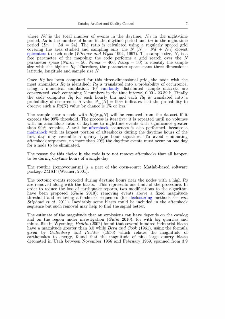
Gulia (2010) suggested removing the aftershock sequences before applying the Wiemer and Baer (2000) algorithm because the removal of events above a fixed magnitude inevitably interferes with the identification of the sequences by the code. Indeed the new catalog contains now only events in the range minimum magnitude- maximum explosion threshold magnitude and mainshock-aftershocks sequences are then modified. A second limit of the algorithm is the detection of quarry blasts in countries like Turkey, where the quarries are located in seismically active regions: many quarry blasts are included in aftershock sequences or in seismic swarms. In such cases, the code can be used to identify areas with a high Rq, where a more specific microseismicity study should be performed. High quality catalogs might include quarry blasts. Examples of Rq maps for Italy (CSI 1.1, Castello et al. 2006; on the left) and France (http://renass.u-strasbg.fr/, on the right) are shown in Fig. 3. The average value in the Rq maps is about 1, but some points have a high Rq

value (≥ 1.5). The histograms of the number of events as a function of hour of the day and the relative histograms of the number of events for the day of the week for some of the volumes with the highest Rq are also shown: in such areas the events have been mainly recorded during daytime (i.e., working time) and during the working days. In the location number 2 and 3 a decrease during lunch break time (12-14) is also observed.

Catalog Artifact and Quality Control 9

Fig. 3 Rq maps for the Italian (left) and French (right) catalogs and histograms of the number of events as a function of hour of the day and the relative histograms of the number of events for the day of the week for 3 of the points with the highest Rq values. In location 1, events occur almost exclusively at the beginning of work in the morning and almost never on Sundays. In location 2 most events are recorded at the beginning and end of working hours. At location 3 in France events on weekends are conspicuously absent.

10 www.corssa.org

4.3 Differences in reporting resolution in earthquake catalogs

Resources to operate seismograph networks change as a function of time, and the availability of locations suitable for deploying instruments varies as a function of space and priorities. Consequently, the resolution of reported earthquakes is heterogeneous in time and space. However, for statistical analysis, the minimum magnitude reported completely, Mc, must be homogeneous throughout the data set; otherwise spurious results may lead to incorrect conclusions. Here, we examine the catalog for central Italy, as defined in Figure 4 to illustrate heterogeneities of Mc. This dataset contains 17,548 events with magnitudes.

Fig. 4 Epicenter map of all earthquakes reported in Central Italy during the period 1981 through 2002.

4.3.2 Heterogeneity of Mc as a function of time

As a first step, we investigate changes of Mc as a function of time, using the computer tool ZMAP (Wiemer 2001). Changes clear to the eye occurred at the beginning of 1989 and at the end of 1997 (Fig. 5). The first gradual decrease in Mc is most likely caused by the gradual improvement and buildup of the network and processing tools. The peak in Mc around 1997 is caused by the numerous aftershocks following the Umbria-Marche sequence (Ml 5.6 and 5.8 on 26 September 1997. After the Umbria-Marche sequence, the Italian seismic network was upgraded, leading to an improvement in Mc (Amato and Mele 2008)

Catalog Artifact and Quality Control 11

Fig. 5 Average minimum magnitude of complete reporting as a function of time, using 500 events per sample and the point of maximum curvature for definition. Dashed lines indicate one standard deviation from the average (bootstrap from Wiemer and Woessner, 2005).

Although the amplitudes of these changes are relatively small (0.2 and 0.1 units in 1989 and 1997, respectively), they exceed one standard deviation. We used only epicenters located on land because the offshore catalog has different properties than the one on land, as will be shown in the following. Mc-values within each of the three periods are fairly constant, so that we may reasonably treat them as samples for which we may plot meaningful frequency magnitude distributions (FMDs). Fig. 6 shows that the values of Mc in the three periods (1981-1989, 1989-1997.7, and 1998.5- 2002.9) are well defined and measure 1.9, 1.7, and 1.6, respectively, as expected from inspection of Fig. 5.

Fig. 6 Frequency magnitude distribution for epicenters on land in central Italy, as defined in Fig. 7 for the three periods that stand out as different from each other in Fig. 8.

4.3.3 Heterogeneity of Mc as a function of space

Almost all operators of seismograph networks report events within and outside the area covered by their instruments. Mc within and outside is rarely the same. If it is, the job done on the inside is poor. ZMAP offers an option to map Mc as a

12 www.corssa.org

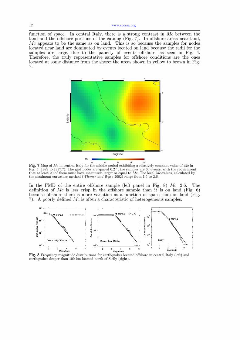
function of space. In central Italy, there is a strong contrast in Mc between the land and the offshore portions of the catalog (Fig. 7). In offshore areas near land, Mc appears to be the same as on land. This is so because the samples for nodes located near land are dominated by events located on land because the radii for the samples are large, due to the paucity of events offshore, as seen in Fig. 4. Therefore, the truly representative samples for offshore conditions are the ones located at some distance from the shore; the areas shown in yellow to brown in Fig. 7.

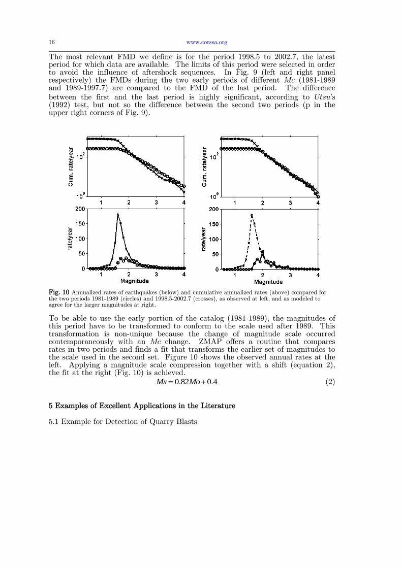
Fig. 7 Map of Mc in central Italy for the middle period exhibiting a relatively constant value of Mc in Fig. 5 (1989 to 1997.7). The grid nodes are spaced 0.2º, the samples are 60 events, with the requirement that at least 20 of them must have magnitude larger or equal to Mc. The local Mc-values, calculated by the maximum curvature method (Wiemer and Wyss 2002) range from 1.6 to 2.6. In the FMD of the entire offshore sample (left panel in Fig. 8) Mc=2.6. The definition of Mc is less crisp in the offshore sample than it is on land (Fig. 6) because offshore there is more variation as a function of space than on land (Fig. 7). A poorly defined Mc is often a characteristic of heterogeneous samples.

Fig. 8 Frequency magnitude distributions for earthquakes located offshore in central Italy (left) and earthquakes deeper than 100 km located north of Sicily (right).

Catalog Artifact and Quality Control 13

Samples of deep earthquakes show high Mc-values because the distance to the nearest seismographs is large. In southern Italy the ensemble of events deeper than 100 km shows Mc=3.5 (central panel of Fig. 8). The boundaries of the lower quality offshore and deep catalog portions are easily defined. However, quality differences in resolution exist within the on-land catalog also. As an example, plotting the shallow seismicity of Sicily, one finds that Mc=3.2 (right panel of Fig. 8).

4.3.4 Discussion of Mc-Heterogeneity

The heterogeneities of Mc shown here to exist in the Italian earthquake catalog are quite clear as a function of time and space. As a function of time, the difference is 0.3 units between the beginning and the end of the catalog (Figs. 5 and 6) because detection has improved. The difference in Mc between the onshore and offshore portions of the catalog is 0.9 units (central panel of Fig. 6 compared to left panel of Fig. 8). This difference is strong enough that one should consider the two samples as different catalogs. The same is true for deep earthquake for which the Mc differs by 1.8 units from the resolution observed in central Italy (central panel of Fig. 8 compared to right panel of Fig. 6). Mixing the offshore or the deep catalog with the shallow onshore, one does no harm, if the investigation centers on shallow onshore earthquakes because the latter contains three orders of magnitude more events than the other sets together, completely dominating the results. However, properties of offshore earthquakes or deep ones cannot be studied, unless they are separated from the onshore shallow events. Misleading results and incorrect interpretation may be obtained if samples of similar numbers of events near the coast, but off- and onshore, are mixed (Wiemer and Wyss 2002, 2003). We have not mapped the boundary between the high resolution (Mc=1.6 to 1.7) catalog of central Italy and other parts where Mc is higher because this is not a research paper. However, using the example of Sicily we have shown that some parts of the Italian catalog are much inferior in reporting resolution; Mc=3.2 in Sicily. It would be useful to know what the reporting resolution is in different parts of Italy. The strategy in selecting the subset of a catalog to be studied should aim at defining the area and period in which the reporting is homogeneous and which contains a maximum number of events. The maximum number gives the most detailed resolution of the parameter to be measured in time and space, and it also affords the strongest statistical power. Starting the catalog at early times and covering a wide area requires selection of a relatively large Mc. Using a large Mc may delete more earthquakes than we gain by the long period and the large area.

14 www.corssa.org

The numbers of earthquakes we retain for analysis by defining the limits of the homogeneous dataset in different ways in our examples from Italy are summarized in Table 1.

Case Mc Period N Fraction (%) Dataset for Analysis

1 1.9 1981-2003 7,582 100 entire period

2 1.7 1989-2003 6,045 80 period restricted to Mc≥1.7

3 1.6 1998.5-2003 1,477 19 period restricted to Mc≥1.6

4 2.6 1981-2003 1,727 23 allowing inclusion of offshore

5 3.5 1981-2003 257 3 allowing inclusion of deep

6 -1.0 1981-2003 17,548 231 all events with M in the catalog

7 all 1981-2003 40,536 535 including events without M

Table 1. Fraction of reported events useful for analysis by subset for the catalog for on-land epicenters in central Italy

The reference data set, to which we assign 100% for the numbers it contains, shall be the subset of the on-land events in central Italy for the whole period (case 1 in Table 1). If we needed, for some reason, to include the offshore area in our study, Mc would have to be raised to 2.6, which would reduce the number of events on land to 1,727, only 23% of the otherwise available data (case 4). The case 4 offers so few events for study that one would avoid extending the study area beyond the coast, if possible. In case 2 one gains events for the study by decreasing Mc to 1.7, but one loses more by starting it in 1989 only, instead of in 1981, ending up with a dataset containing only 80% as many events as case 1. This is a bit unusual; most often it pays to start later and use lower Mc-values. In central Italy, the subset that would require an even higher, unfavorable Mc is that before 1981 and is already excluded. The strategy to use the period with the best resolution (Mc=1.6) for analysis would lead to a dataset containing only 19% of the available data because the period covered is short. Thus, case 3 is not a viable option. For sake of argument, we ask the question: What portion of the case 1 data would we lose, if we wanted to study it together with earthquakes deeper than 100 km reported for Italy? In this case 5, we would lose 97% of the data (Table 1). On the side, we note that the number of earthquakes including all magnitudes in the catalog for central Italy (case 6, Table 1) is about 2.3 times larger than the

number of events with Mc>1.9. Furthermore, the total number of reported events in the catalog, including those without magnitude (case 7), is approximately 5.4 times as large as the maximum dataset useful for statistical studies (case 1). These data sets including small magnitude events and those without magnitudes cannot be used for statistical analyses.

Catalog Artifact and Quality Control 15

4.3.5 Conclusions Concerning Mc-Heterogeneity

This section does not address actual research problems but data requirements that must be fulfilled, if one wants to avoid spurious results. We recommend that before any statistical analysis the following main points be considered to insure that one works with a catalog in which reporting is homogeneous.

The quality of reporting as reflected by the local Mc-values varies in almost all earthquake catalogs as a function of space and time.

For statistical analyses, the data set must be homogeneous in Mc.

Changes of Mc as a function of time should be identified in a first step of defining the highest quality subset of a catalog, useful for statistical analysis.

Differences of Mc as a function of space should be mapped for a period of constant Mc-resolution, in a second step.

The sub-catalog best suited for answering the problem at hand and having the strongest power of statistical resolution should be selected by culling the total catalog in time and space.

4.4 Differences in Magnitude Scales in Earthquake Catalogs

The attentive reader may have noticed that at the times of changes in Mc (Fig. 5) the b-values seem to have changed also (Fig. 6). The hypothesis is not attractive that the b-value has changed due to natural causes simultaneous in a large part of Italy and at the same time as Mc has changed. If the change is significant, it is most likely that the magnitude scale was changed inadvertently.

Fig. 9 Comparison of b-values for earthquakes in central Italy on-land. The limiting dates used are given at the top right without the century. The numbers in the samples and the b-estimates are given as n and b, respectively, with the index 1 and 2 signifying the two periods. The probability that the two samples come from the same distribution is given as p. Solid dots mark the most recent data.

16 www.corssa.org

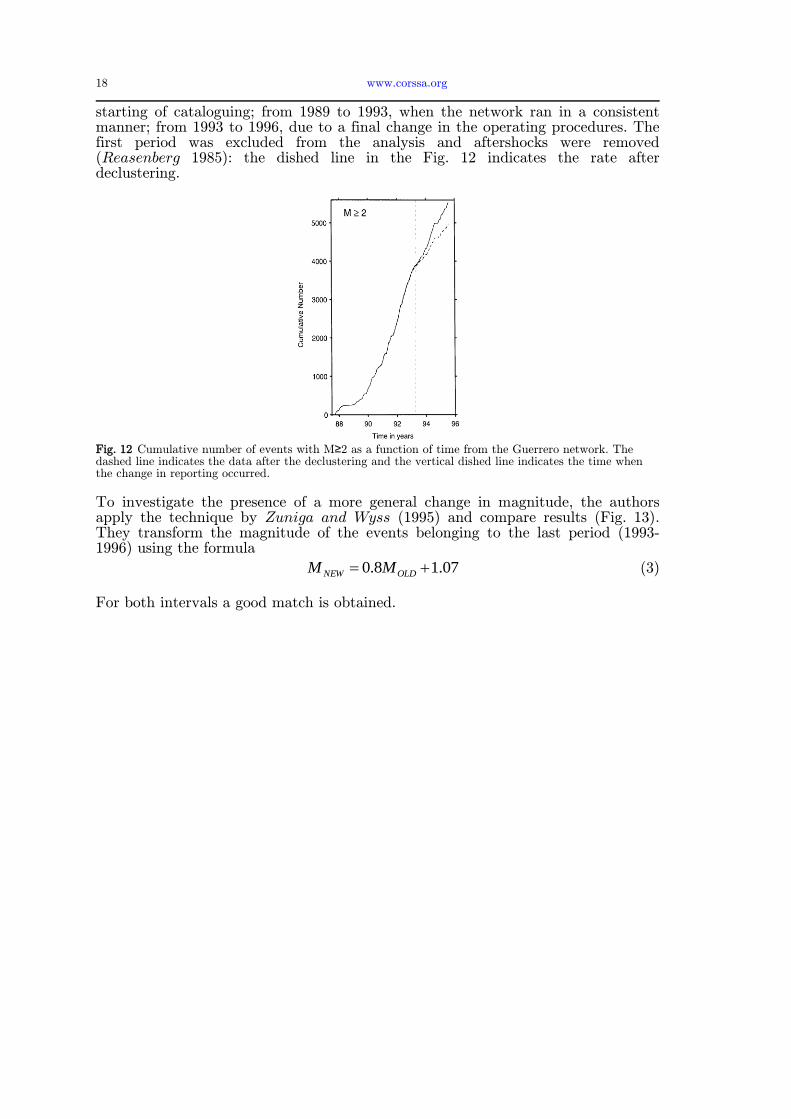
The most relevant FMD we define is for the period 1998.5 to 2002.7, the latest period for which data are available. The limits of this period were selected in order to avoid the influence of aftershock sequences. In Fig. 9 (left and right panel respectively) the FMDs during the two early periods of different Mc (1981-1989 and 1989-1997.7) are compared to the FMD of the last period. The difference

between the first and the last period is highly significant, according to Utsu’s (1992) test, but not so the difference between the second two periods (p in the upper right corners of Fig. 9).

Fig. 10 Annualized rates of earthquakes (below) and cumulative annualized rates (above) compared for the two periods 1981-1989 (circles) and 1998.5-2002.7 (crosses), as observed at left, and as modeled to agree for the larger magnitudes at right.

To be able to use the early portion of the catalog (1981-1989), the magnitudes of this period have to be transformed to conform to the scale used after 1989. This transformation is non-unique because the change of magnitude scale occurred contemporaneously with an Mc change. ZMAP offers a routine that compares rates in two periods and finds a fit that transforms the earlier set of magnitudes to the scale used in the second set. Figure 10 shows the observed annual rates at the left. Applying a magnitude scale compression together with a shift (equation 2), the fit at the right (Fig. 10) is achieved.

4.082.0 MoMx (2)

5 Examples of Excellent Applications in the Literature

5.1 Example for Detection of Quarry Blasts

Catalog Artifact and Quality Control 17

Wiemer and Baer (2000) analyze the seismicity catalog compiled by the Swiss Seismological Survey during the period January 1980-December 1998, that contains approximately 5500 earthquakes (Deichmann 1992; Baer et al. 1997). Fig. 11 shows the Rq map and the hourly histogram of the number of events for the original catalog (a) and after the removal of quarry blasts (b). Comparison with the location of known quarries confirms that the areas with a high Rq are likely locations for quarry blasts. About 20% of events were removed from the data set.

Fig. 11 (Left) Map of the ratio of daytime to nighttime events (Rq) for Switzerland. This map was produced by gridding the seismicity, using a 10 km node spacing, and sampling the 100 nearest events to each node. Rq values greater than 1 indicate the presence of quarries. (Right) Hourly histogram of the number of events (a) for the original catalog and (b) after removing explosions.

5.2 Examples for Magnitude Changes

Zuniga and Wiemer (1999) analyze data from one local (Guerrero Gap, Mexico) and one regional catalog (interior of Alaska) demonstrating how artificial seismicity patterns may arise due to changes in magnitude reporting. They use and compare two different techniques:

1. the systematic comparison of the cumulative and non-cumulative frequency-magnitude distribution for two periods;

2. the quantitative mapping of seismicity rates as a function of time and space. Results are obtained through the ZMAP software (Wiemer 2001). Here we show the case study of Mexico. The network used for the catalog of Guerrero (Institute of Geophysics of the National University of Mexico) has been subjected to various changes in time: all the stations were installed in 1987 but not all have been in operation continuously. Fig. 12 shows the seismicity rates for events with a

magnitude M≥ 2, lower than the magnitude of completeness (about 2.5 from the b-value distribution). Three main trends can be seen: from 1987 to 1989, due to the

18 www.corssa.org

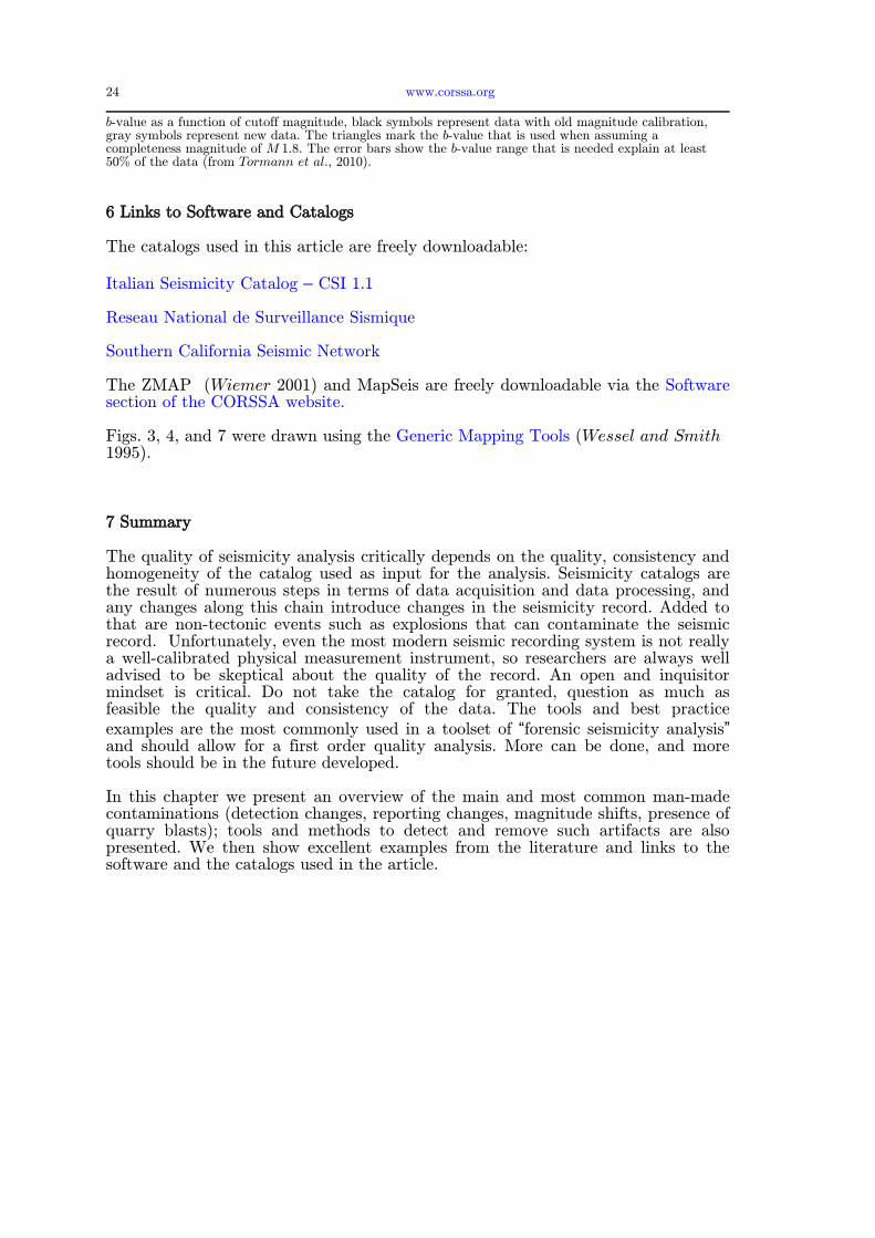
starting of cataloguing; from 1989 to 1993, when the network ran in a consistent manner; from 1993 to 1996, due to a final change in the operating procedures. The first period was excluded from the analysis and aftershocks were removed (Reasenberg 1985): the dished line in the Fig. 12 indicates the rate after declustering.

Fig. 12 Cumulative number of events with M≥2 as a function of time from the Guerrero network. The dashed line indicates the data after the declustering and the vertical dished line indicates the time when the change in reporting occurred. To investigate the presence of a more general change in magnitude, the authors apply the technique by Zuniga and Wyss (1995) and compare results (Fig. 13). They transform the magnitude of the events belonging to the last period (1993-1996) using the formula

07.18.0 OLDNEW MM (3)

For both intervals a good match is obtained.

Catalog Artifact and Quality Control 19

Fig. 13. Cumulative number of events (a and b) and non-cumulative number of events (c and d) as a function of magnitude. The frames a and c refer to the original dataset, the frames b and d to the corrected one (from Zuniga and Wiemer 1999). Finally the authors analyze the spatial dependency of rate changes by comparing the seismicity rates within a selected time window and the seismicity rates of the entire catalog, excluding the analysis window. The area is subdivided in a densely spaced grid and for each grid node the 300 nearest earthquakes are selected. A statistical z-test using the LTA(t) function (Long Term Average, Habermann 1987; Wiemer and Wyss 1994) is carried out for each time series at each node. Figure 14 shows the maps of the standard deviate z for four different periods (the original data on the left, the corrected data on the right). The eight maps show the rate variation of one year, starting at the beginning of each year, from 1990. Positive z-values indicate a rate decrease and negative values an increase: the apparent decrease shown by the original dataset is enhanced by the correction.

20 www.corssa.org

Fig. 14. Maps of the standard deviate z for four different times. On the left the original data, on the right

the corrected ones. Positive z-values indicate a rate decrease (see text; from Zuniga and Wiemer 1999)

Tormann et al. (2010) offer another excellent example of how the change in magnitude calibration may affect seismicity analyzing the Southern California Seismic Network (SCSN). Starting January 2008, local magnitudes ML for southern California are determined by a new calibration. Magnitudes for the previous years are being recalculated and the first year of overlapping data now being available. Tormann et al. (2010) compared the old and the new ML for the year 2007.

We here briefly show their results:

1. The two magnitude values differ for 96% of the ML events and the differences are irregular from magnitude increases of up to 1.5 units to reductions by as much as 2.3 units, with an average change of -0.13 units. For each event (Fig. 15 a-f) the authors plot the new versus the old magnitude and include via grayscale the frequency of observation: most of the magnitude values are reduced.

Catalog Artifact and Quality Control 21

Fig. 15 (a-c) Subplots show the new versus the old magnitude data for all magnitude types. The grayscale values of the data points show per magnitude bin the fraction of the old magnitude events in this bin that have been assigned the new magnitude shown at each point. For each magnitude bin from the old scale Tormann et al. (2010) count the number of events in the old catalog and divide the number of observations for each of the new magnitudes by this total bin number. The straight lines are the lines of equal magnitudes. (d-f) Subplots show the magnitude histograms for the old (dashed) versus the new (solid) magnitude data (from Tormann et al. 2010).

2. The number of events above M 1.8 decreases by 32% for the new magnitude scale: changes in the magnitude scale can indeed result in a rate change for certain magnitude bands. To measure the significance of the rate changes, Tormann et al. (2010) first calculate the percentage of change in the numbers of new versus old data for all magnitude cutoffs from M0 toM4.0 in 0.1 magnitude steps (Fig. 16). For each magnitude cutoff they calculate the Poisson probability that the change could have been observed by chance. The observed rate changes in Figure 15 are

22 www.corssa.org

grayscale-coded by the confidence to which a random occurrence based on their Poisson probability values can be excluded. Confidence values of more than 99.99% (dark gray) are statistically significant changes in the seismicity rate reporting. For cutoff magnitudes between M 0.5 and M 2.2 they find highly significant rate decreases, with the maximum decrease of 33% for M 1.6.

Fig 16. Observed rate changes between old and new data for 2007 and their significances for cutoff magnitudes M 0.1 to M 4.0. Rate changes annotated in light gray are within 90% confidence limits and are insignificant, medium gray bars have significance values between 90% and 99.99%, and rate changes in

Catalog Artifact and Quality Control 23

dark gray have statistically highly significant values with more than 99.99% confidence; the probability of an observation by chance is less than 0.01% for these changes (from Tormann et al. 2010). 3. The completeness magnitude apparently drops by 0.3 units from 1.6 to 1.3. The magnitude of completeness has been determined by the EMR (Woessner and

Wiemer 2005) for the two catalogs for 2007 for all events with M>0. 4. The b-value reduces by approximately 0.2 units, dropping from 1.16 to 0.95. Tormann et al. (2010) calculate the b-values for both versions of the catalog for 2007 as well as a nearly continuous temporal evolution for 2002 to 2008. They assume M 1.8 to be the magnitude of completeness in the study region, using

Mmin equals 1,8 – 0,05 and the data sets’ mean magnitudes Mmean to compute maximum-likelihood b-values (Utsu 1965, Aki 1965, Bender 1983). The confidence limit of this estimation is given by Shi and Bolt (1982). They also calculate the b-values for a 600-event window with an overlapping of 120 events to relate such changes to the temporal fluctuation over the period 2002-2008 (Fig. 17a). Data before 2007 are computed with the old magnitude calibration (black in Fig. 17a); for 2007 both values are available, for 2008 onward only the new values (gray in

Fig. 17a). The mean b-value calculated from old magnitude data (2002–2007) is 1.1

+/- 0.01; for the new magnitude data (2007–2008) it is 0.94 +/- 0.02. 5. The new magnitude calibration produces a more stable b-value estimate and can therefore be regarded as the better scaling. The last result by Tormann et al. (2010) is shown in Fig. 17b by the well-defined plateau obtained for the frequency-magnitude distribution of the dataset with the new magnitude scale. The presence of a plateau defines the stability and quality of the b-value and can be used to estimate the goodness of scaling in the catalog. The b-values for the old magnitude data are unstable, and do not even form a plateau.

Fig. 17 (a) Temporal evolution of b-values, calculated from 600 events (with 120 events overlap). Tormann et al. (2010) assume a completeness magnitude of M 1.8. Horizontal bars represent the time interval used for each calculation, while vertical bars represent the confidence limits of b, following Shi and Bolt (1982). The black data are calculated from the old magnitudes, the gray data are based on the new

calibration. Dotted lines show the mean b-values calculated for 2002–2007 and 2007–2008, respectively. (b)

24 www.corssa.org

b-value as a function of cutoff magnitude, black symbols represent data with old magnitude calibration, gray symbols represent new data. The triangles mark the b-value that is used when assuming a completeness magnitude of M 1.8. The error bars show the b-value range that is needed explain at least 50% of the data (from Tormann et al., 2010).

6 Links to Software and Catalogs

The catalogs used in this article are freely downloadable:

Italian Seismicity Catalog – CSI 1.1 Reseau National de Surveillance Sismique Southern California Seismic Network The ZMAP (Wiemer 2001) and MapSeis are freely downloadable via the Software section of the CORSSA website. Figs. 3, 4, and 7 were drawn using the Generic Mapping Tools (Wessel and Smith 1995).

7 Summary

The quality of seismicity analysis critically depends on the quality, consistency and homogeneity of the catalog used as input for the analysis. Seismicity catalogs are the result of numerous steps in terms of data acquisition and data processing, and any changes along this chain introduce changes in the seismicity record. Added to that are non-tectonic events such as explosions that can contaminate the seismic record. Unfortunately, even the most modern seismic recording system is not really a well-calibrated physical measurement instrument, so researchers are always well advised to be skeptical about the quality of the record. An open and inquisitor mindset is critical. Do not take the catalog for granted, question as much as feasible the quality and consistency of the data. The tools and best practice

examples are the most commonly used in a toolset of “forensic seismicity analysis” and should allow for a first order quality analysis. More can be done, and more tools should be in the future developed. In this chapter we present an overview of the main and most common man-made contaminations (detection changes, reporting changes, magnitude shifts, presence of quarry blasts); tools and methods to detect and remove such artifacts are also presented. We then show excellent examples from the literature and links to the software and the catalogs used in the article.

Catalog Artifact and Quality Control 25

References Amato A. and F.M. Mele (2008) Performance of the INGV National Seismic Network from 1997 to 2007,.

Annals of Geophysics, vol. 51(2/3), 417-431

Aki, K. (1965), Maximum likelihood estimate of b in the formula logN =a –bM and its confidence limits,

Bull. Earthq. Res. Inst. 43, 237–239 Baer, M., N. Deichmann, D. Faeh, U. Kradolfer, D. Mayer-Rosa, E. Ruettener, T. Schler, S. Sellami, and

P. Smit (1997). Earthquakes in Switzerland and surrounding regions during 1996, Eclogae Geol. Helv. 90, 557– 567.

Bath M. (1975), Short-period Rayleigh waves from near-surface events, Phys Earth Planet Inter, 10, 369{376

Bender, B. (1983), Maximum likelihood estimation of b-values for magnitude grouped data, Bull. Seismol.

Soc. Am. 73, 831–851. Berg, J.W. and K.L. Cook (1961), Energies, Magnitudes and Amplitudes of Seismic Wawes from quarry

blasts at Promontory and Lakeside, Utah., Bull Seism Soc Am 51(3), 389{399

Castello, B., G. Selvaggi, C. Chiarabba and A. Amato, (2006) CSI Catalogo della sismicità italiana 1981-2002, versione 1.1. INGV-CNT, Roma, Available via DIALOG: http://www.ingv.it/CSI/

Deichmann, N. (1992). Structural and rheological implications of lower crustal earthquakes below northern Switzerland, Phys. Earth Planet. Interiors 69, 270– 280.

Giardini, D., S. Wiemer, D. Fä h, D. Deichmann (2004), Seismic Hazard Assessment of Switzerland. Report, Swiss Seismological Service, ETH Zurich, 88 pp.

Gulia, L. (2010), Detection of quarry and mine blast contamination in European regional catalogues, Nat. Hazards, 53, 229{249, DOI 10.1007/s11069-009-9426-8

Gutenberg, B. and C.F. Richter (1956) Earthquake, Magnitude, Intensity and Acceleration (second paper), Bull. Seism. Soc. Am., 46, 105{143

Habermann, R.E. (1986), A test of two techniques for recognizing systematic errors in magnitude estimates using data from Parkfield, California, Bull. Seism. Soc. Am., 76 (86), 1660{1667.

Habermann, R.E. (1987), Man-made changes of seismicity rates, Bull. Seism. Soc. Am., 77 (1), 141{159. Hedlin, M.A. (2002), Identification of Mining Blasts at Mid- to Far-regional Distances Using Low

Frequency Seismic Signals., Pure appl Geophys, 159, 831{863 Horasan, G., A.B. Guney, A. Kusmezer, F. Bekler, Z. Ogutcu and N. Musaoglu (2009), Contamination of

seismicity catalogs by quarry blasts: an example from Istanbul and its vicinity, northwestern Turkey, J Asian Earth Sci 34(1), 90{99.

Kafka, A.L. (1990), Rg as a depth discriminant for earthquakes and explosions: a case study in New England, Bull. Seism. Soc. Am., 80(2), 373{394

Koch K. and D. Fah (2002), Identification of earthquakes and explosions using amplitude ratios: The Vogtland area revisited. Pure Appl. Geophys. 159,735{757

Murphy J.R., Bennet T.J., 1982. Analysis of seismic discrimination capability using regional data from Western United States events, Bull Seism Soc Am, 76, 1069{1086

Musil M. and A. Plešinger (1996). Discrimination between local microearthquakes and quarry blasts by multilayer perceptrons and Kohonen Maps, Bull. Seism. Soc. Am. 86(4), 1077{1090

Oncescu, M.C., V.I. Marza, M. Rizescu and M. Popa, (1999), The Romanian Earthquake Catalogue between 984-1997, In: F. Wenzel, D. Lungu (eds.) and O. Novak (co-ed), Vrancea Earthquakes: Tectonics, Hazard and Risk Mitigation, Kluwer Academic Publishers, Dordrecht, Netherlands, pp. 43-47

Parolai S., L. Trojani, M. Frapiccini, G. Monachesi (2002), Seismic source classification by means of a sonogram-correlation approach: application to data of the RSM seismic network (Central Italy). Pure Appl. Geophys. 159, 2763{2788

Reasenberg P.A. (1985), Second-Order Moment of Central California Seismicity, J. Geophys. Res., 90, 5479-5495.

Shi, Y., and B. A. Bolt (1982), The standard error of the magnitude frequency b value, Bull. Seismol. Soc.

Am. 72, 1677–1687. Tormann T., S. Wiemer, E. Hauksson E. (2010), changes in reporting Rates in the Southern California

Earthquake Catalog, Introduced by a New Definition of Ml, Bull. Seism. Soc. Am. 100(4), 1733{1742 Utsu, T., (1992). On seismicity. in Report of the Joint Research Institute for Statistical Mathematics, pp.

139-157Institute for Statistical Mathematics, Tokyo. Utsu, T. (1965).,A method for determining the value of b in a formula log n = a - b M showing the

magnitude frequency for earthquakes, Geophys. Bull. Hokkaido Univ. 13, 99– 103. van Stiphout, T., Zhuang, J., Marsan, D. (2010), Seismicity Declustering, Community Online Resource for

Statistical Seismicity Analysis, doi:10.3929/ethz-a-xxxxxxxxx. Available at http://www.corssa.org.

26 www.corssa.org

Wessel, P. and W.H.F. Smith (1995), New version of the generic mapping tools released, Eos. Trans., 76, 329.

Wiemer S. (2001), A software package to analyze seismicity: ZMAP, Seismol Res Lett 92, 373-382 Wiemer S. and M. Wyss (1994), Seismic Quiescence before the Landers (M=7.5) and Big Bear (M=6.5)

1992 Earthquakes, Bull. Seismol. Soc. Am., 84, 900-916. Wiemer, S and M. Wyss (1997), Mapping the frequency-magnitude distribution in asperities: an improved

technique to calculate recurrence times?, J. Geophys. Res., 102, 15115{15128. Wiemer S. and M. Wyss (2002), Mapping Spatial variability of the Frequency-magnitude distribution of

Earthquake, Adv. Geophys., 45, 259-302.

Wiemer S. and M. Wyss (2003), Reply to the comments by Rydelek and Sacks on ‘Minimum magnitude of complete reporting in earthquake catalogs: examples from Alaska, the Western United States, and

Japan‘ Bull. Seism. Soc. Am., 1868-187. Wiemer S. and M. Baer (2000), Mapping and removing quarry blast events from seismicity catalogs, Bull.

Seism. Soc. Am., 90(2), 525{530 Woessner J. and S. Wiemer (2005), Assessing the quality of earthquake catalogues: Estimating the

magnitude of completeness and its uncertainty. Bull. Seismol. Soc. Am., 95, doi: 10.1785/012040.007 Woessner J., J. Hardebeck, E. Hauksson (2011), What is an instrumental seismicity catalog? Community

Online Resource for Statistical Seismicity Analysis, doi:10.50787corssa-38784307. Available at hppt://www.corssa.org

Wuster J. (1993), Discrimination of chemical explosions and earthquakes in Central Europe—a case study, Bull. Seism. Soc. Am., 83(4), 1184{1212

Wyss, M., F.W. Klein, A.C. Johnston (1981), Precursors to the Kalapana M=7.2 earthquake, J. Geophys. Res., 86, 881{ 3900.

Wyss, M., R.E. Habermann and C. Heiniger (1983), Seismic quiescence, stress drop and asperities in the New Hebrides arc, Bull. Seism. Soc. Am., 73, 219{236.

Wyss, M., R.E. Habermann and J.-C. Griesser (1984), Seismic quiescence and asperities in the Tonga-Kermadec Arc, J. Geophys. Res., 89, 9293{9304.

Zuniga F.R. and S. Wiemer (1999), Seismicity Patterns. Are They Always Related to Natural Causes? Pure appl. Geophys., 155, 713-726.

Zuniga F.R. and M. Wyss (1995), Inadvertent Changes in Magnitude Reported in Earthquake Catalogs: Their Evaluation Trough b-value Estimates, Bull. Seismol. Soc. Am., 85, 1858-1866.