THE DYNAMO EFFECT

S. FAUVE AND F. PETRELIS

LPS, Ecole normale superieure,

24, rue Lhomond,

75005 Paris, France

E-mail: fauve@lps.ens.fr

We first present basic results about advection, diffusion and amplification of a

magnetic field by the flow of an electrically conducting fluid. This topic has beeninitially motivated by the study of possible mechanisms to explain the magneticfields of astrophysical objects. However, self-generation of a magnetic field byan electrically conducting fluid, the so-called dynamo effect, is also a typical bi-furcation problem that involves many interesting aspects from the viewpoint ofdynamical system theory: the effect of the flow geometry on the nature of the bi-furcation, the effect of turbulent fluctuations on the threshold value, the saturation

mechanisms above threshold, the dynamics of the generated magnetic field and thestatistical properties of its fluctuations with respect to the ones of the turbulent

flow. We have tried to emphasize some of these problems within the general pre-sentation of the subject and more particularly in sections 6 and 7. These notes

should not be considered as a review article. There exist many well known booksand reviews on dynamo theory 1,2,3,4,5,6. For a general presentation of the sub-

ject, we refer to “Magnetic field generation in electrically conducting fluids” byMoffatt 7. The generation of large scale magnetic fields by small scale turbulentmotions is reviewed in “Mean-field magnetohydrodynamics and dynamo theory”by Krause and Radler 8. The problem of “fast dynamos” in the limit of large

magnetic Reynolds number is studied by Childress and Gilbert in “Stretch, twist,

fold: the fast dynamo” 9. Finally, we refer to “Magnetic fields in astrophysics” by

Zeldovich, Ruzmaikin and Sokoloff 10 for a detailed review on magnetic fields ofastrophysical objects and their possible role in the early evolution of the universe.

1. Introduction: from industrial dynamos to the magnetic

field of stars and planets

1.1. Generation of an electric current by a rotating

conductor

The generation of an electric current from mechanical work is a very com-

mon process. Most of the electric energy we are using on the Earth has

been transformed from mechanical energy at some stage. It is however

not always understood that the elementary process that allows the trans-

1

2

formation of mechanical work into electromagnetic energy is an instability

mechanism.

It has been known since Faraday that it is possible to generate an elec-

tric current by rotating an electrically conducting disk of radius a in an

externally applied magnetic field ~B0 (see Figure 1 a). Indeed, the electro-

motive force e between the points A and P can be easily computed from

the law of induction

e =

∫

AP

(

(~Ω× ~r)× ~B0

)

· d~r = 1

2Ωa2B0, (1)

and generates a current I = e/R in the electric circuit of resistance R. Is

it possible to use this current to generate the magnetic field ~B0 ? This

may look a strange question but leads to a typical instability problem. The

answer is yes if the geometry of the circuit is such that a perturbation of

the electrical current generates a magnetic field which amplifies the current

by electromagnetic induction. An experimental demonstration of this type

of effect was first performed by Siemens 11 and gave rise to various devices

widely used to generate an electrical current from mechanical work. The

simplest although non efficient way to achieve self-generation of a current

or a magnetic field is the homopolar dynamo displayed in Figure ( 1 b)

(sometimes called the Bullard dynamo in the english literature). Ohm’s

law gives

LdI

dt+RI = e = MΩI, (2)

where L is the induction of the circuit and M is the mutual induction

between the wire and the disk. Indeed, from equation (1) it follows that

e is proportional to Ω and I that generates the magnetic field ~B. Using

equation (2), the stability analysis of the solution I = 0 (corresponding to

B = 0) is straightforward. The current I and thus the magnetic field B are

exponentially amplified if

Ω > Ωc =R

M. (3)

It first appears that the self-generation of current depends on the sign

of the rotation rate. This is not very surprising because the wire breaks the

mirror symmetry with respect to any plane containing the axis of rotation.

The sign of the wire helicity gives the sign of M and thus determines the

sign of Ω for self generation. Note that if we add a second wire of opposite

helicity parallel to the first one such that the device becomes mirror sym-

metric, then M = 0 and self-generation of current is no longer possible. We

3

A

P

B

I

Ωo

A

P

B

I

Ω

(a)

(b)

Figure 1. (a) Sketch of the Faraday inductor. (b) Sketch of the homopolar dynamo.

will also observe that broken mirror symmetry by the flow is important in

the case of fluid dynamos. We have obtained so far the condition (3) for

the onset of dynamo action. This is called solving the kinematic dynamo

problem. For a rotation rate larger than Ωc, equation (2) seems to indicate

that the current is exponentially growing. This process should stop at some

stage as shown by the equation for the angular rotation rate

JdΩ

dt= Γ−D −MI2, (4)

where J is the moment of inertia of the disk, Γ is the torque of the motor

driving the disk, D represents mechanical resistive torques. The last term is

the torque which results from the Laplace force generated by the magnetic

4

field ~B acting on the current density ~j flowing in the disk∫

~r ×(

~j × ~B)

d3r = MI2 z. (5)

This force is opposite to the motion of the disk and is proportional to I2.

It can be easily checked that the proportionality constant in (5) is M by

looking at the energy budget. To wit, we multiply (2) by I and (4) by Ω

and add them. We obtain

d

dt

1

2

(

JΩ2 + LI2)

= (Γ−D) Ω−RI2. (6)

This equation reflects energy conservation. In a stationary regime, the

power of the motor is dissipated by mechanical losses and Joule heating.

Note that the two contributions proportional to ΩI2 cancel in order to

have energy conservation. The growth of the current is thus limitated by

the available mechanical power. The stationary solutions of equations (2,

4) are

Ω = Ωc =R

M, I =

Γ−D

RΩ =

Γ−D

M. (7)

Finding the generated current or magnetic field is called solving the dy-

namic dynamo problem. The kinematic dynamo problem is thus the linear

stability analysis of the solution B = 0 whereas the dynamic dynamo prob-

lem consists of solving the full nonlinear problem.

In the above simple example, we have a stationary bifurcation for Ω =

Ωc. The broken symmetry at instability onset is the B → −B symmetry

or the I → −I symmetry of equations (2, 4). The bifurcation diagram may

look surprising. The bifurcated branches of solution for I that we expect

for Ω > Ωc are absent. This is because we have neglected all the possible

nonlinear saturation mechanisms (dependence of L or M on B, destruction

of the circuit if I becomes too large, detailed behavior of the motor, etc).

However, this example shows how the dynamo effect allows to generate

electromagnetic energy from mechanical work. A lot of its features will

subsist in fluid dynamos i.e. generation of a magnetic field by the motion

of an electrically conducting liquid.

1.2. Magnetic fields of astrophysical objects

Magnetic fields exist on a wide range of scales in astrophysics. We will just

recall here some results and refer to a review of this topic 10. Orders of

magnitude of the magnetic fields and some associated relevant parameters

for planets, stars and our galaxy are given in Table 1.

5

Table 1. Magnetic fields and fluid parameters of astrophysical objects. All quantities

are given in MKSA units except the magnetic diffusion time L2/νm which is given in

years.

Medium B ρ L νmL2

νm

B2L3

2µ0

B2Lνm2µ0

Our galaxy 10−10 2 10−21 1019 1017 1013 1043 1022

Sun 10−4 1 2 108 103 106 4 1022 109

Jupiter 4 10−4 103 5 107 10 107 1022 4 107

Earth 10−4 104 3 106 3 105 2 1017 105

White dwarfs 102 − 104 1010 107

Neutron stars 106 - 109 1019 104

It is perhaps meaningless to try to compare these data because these

astrophysical objects have strongly different physical properties. A magne-

tohydrodynamic description is probably valid for the Earth core which is

made of liquid metal, but classical hydrodynamics certainly breaks down

both for rarefied plasmas where the mean free path is no longer small com-

pared to the characteristic length on which the velocity varies, and for very

dense stars where quantum and relativistic effects are important (see sec-

tion 2 for a discussion of MHD approximation). If we try anyway to tell

something about these data, we may observe that the magnetic field B is

not strongly related to the size of the object L but seems to increase with

its density ρ. If instead of looking at the intensity of the magnetic field,

we consider the typical magnetic energy of the object B2L3/2µ0 (µ0 is the

magnetic permeability of vacuum), we find the expected ordering from the

galaxy to the Earth. We may also consider the typical value of the Joule

dissipation. To wit, we divide the magnetic energy by the characteristic

magnetic diffusion time L2/νm, with νm = (µ0σ)−1 where σ is the elec-

trical conductivity of the medium. We thus get an idea of the amount

of power which is necessary to maintain the magnetic field against Joule

dissipation. Again, we observe the expected ordering from the galaxy to

the Earth. Note that these powers have been certainly underestimated.

First, they are estimated from the visible part of the magnetic field. If we

consider a celestial body with a nearly axisymmetric mean magnetic field,

as it is often the case, Ampere’s law shows that the azimuthal component

of the magnetic field should vanish out of the conducting medium. If the

azimuthal field inside the body is large compared to the poloidal one, we

may strongly underestimate the total energy or Joule dissipation by taking

the value of the observed poloidal field to evaluate B. Second, we have

assumed that the length scale of the gradients of the magnetic field is the

6

size L of the conducting medium. Magnetic energy at smaller scales will

lead to a shorter diffusion time scale and thus to a higher dissipated power.

However, even if we multiply the dissipated power by a factor 1000, we

still get orders of magnitude rather small compared to the typical energy

budgets of the corresponding astrophysical objects.

The very large astrophysical scales lead to long diffusion times L2/νmfor the magnetic field. On shorter time scales, we may ignore magnetic

diffusivity. The magnetic field is then advected by the flow. If we consider

a field tube of section dS and length dl, the corresponding fluid mass,

ρdSdl, and the flux of the magnetic field, BdS, are conserved. This leads

to B/ρ ∝ dl. For an isotropic compression, we get B ∝ ρ2/3. The “relict

field hypothesis” is based on this argument. It is argued that a very small

intergalactic magnetic field may thus explain the value of the field of our

galaxy. A more detailed analysis seems to rule out this possibility 10. The

situation is clearer for the magnetic fields of the sun or planets. Even

without invoking turbulent diffusivity, the age of the magnetic field of these

objects is in general much larger than their Joule dissipation time scale.

Moreover, these magnetic fields have often a complex dynamics in time and

space: a roughly 22 year oscillation for the sun and random field reversals

for the Earth. Consequently, one should find a field generation mechanism

which involves such dynamics.

1.3. Fluid dynamos

In a short communication made in september 1919, Larmor observed that

the magnetic fields of “celestial bodies” may be generated by internal mo-

tions of conducting matter 12. He emphasized the case of the sun but also

considered the magnetic field of the Earth and ruled out other mechanisms

that were put forward at that time: rotation of an electric polarization

induced either by gravity or centrifugal forces, or of crystalline nature in

the case of the Earth. He explained the fluid dynamo mechanism in a few

lines; assuming the existence of an initial perturbation of magnetic field,

he observed that “internal motion induces an electric field acting on the

moving matter: and if any conducting path around the solar axis happens

to be open, an electric current will flow round it, which may in turn in-

crease the inducing magnetic field. In this way it is possible for the internal

cyclic motion to act after the manner of the cycle of a self-exciting dynamo,

and maintain a permanent magnetic field from insignificant beginnings, at

the expense of some of the energy of the internal circulation. Again, if a

sunspot is regarded as a superficial source or sink of radial flow of strongly

ionized material, with the familiar vortical features, its strong magnetic

7

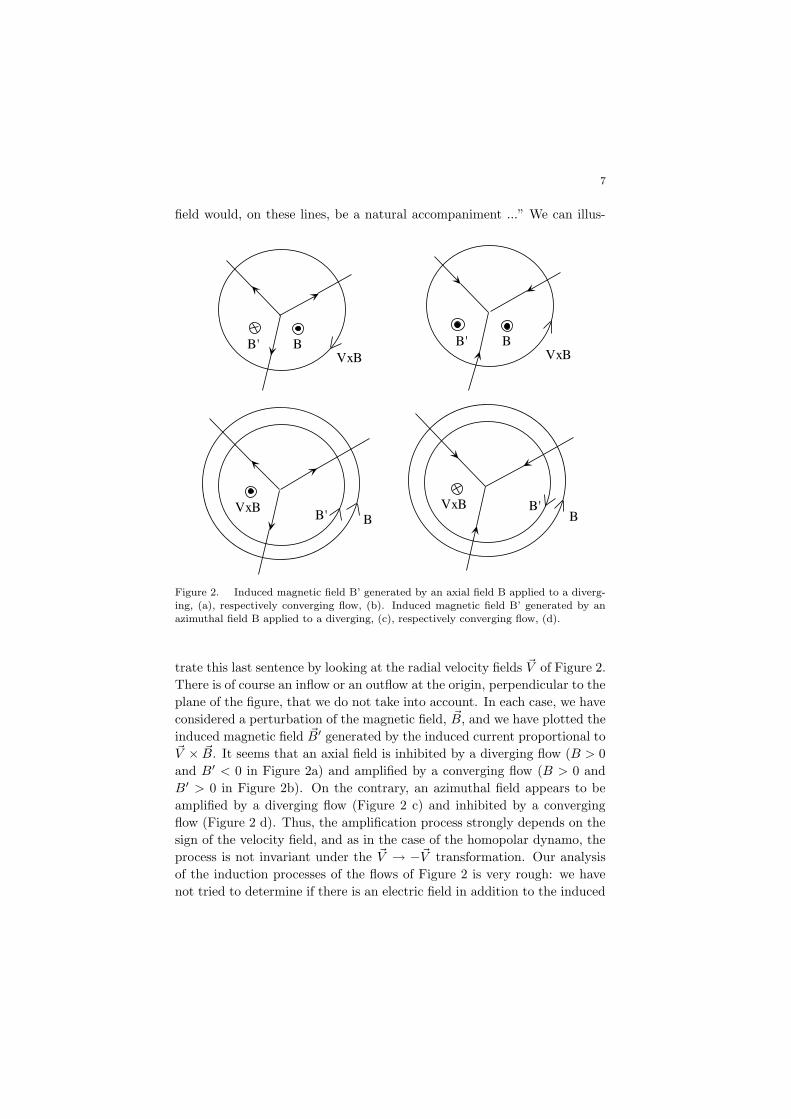
field would, on these lines, be a natural accompaniment ...” We can illus-

BB'VxB

BB'

VxB

BB'

VxB

BB'VxB

Figure 2. Induced magnetic field B’ generated by an axial field B applied to a diverg-ing, (a), respectively converging flow, (b). Induced magnetic field B’ generated by anazimuthal field B applied to a diverging, (c), respectively converging flow, (d).

trate this last sentence by looking at the radial velocity fields ~V of Figure 2.

There is of course an inflow or an outflow at the origin, perpendicular to the

plane of the figure, that we do not take into account. In each case, we have

considered a perturbation of the magnetic field, ~B, and we have plotted the

induced magnetic field ~B′ generated by the induced current proportional to~V × ~B. It seems that an axial field is inhibited by a diverging flow (B > 0

and B′ < 0 in Figure 2a) and amplified by a converging flow (B > 0 and

B′ > 0 in Figure 2b). On the contrary, an azimuthal field appears to be

amplified by a diverging flow (Figure 2 c) and inhibited by a converging

flow (Figure 2 d). Thus, the amplification process strongly depends on the

sign of the velocity field, and as in the case of the homopolar dynamo, the

process is not invariant under the ~V → −~V transformation. Our analysis

of the induction processes of the flows of Figure 2 is very rough: we have

not tried to determine if there is an electric field in addition to the induced

8

~V × ~B field; as said above, we have not taken into account the inflow or

outflow at the origin that would make the flow three-dimensional. However,

we have illustrated with these simple flows what Larmor had already prob-

ably in mind, i.e. that a given flow may amplify some field configurations

and at the same time inhibit some others. The main difficulty is that the

field geometry is not determined by the geometry of the currents like in the

homopolar dynamo or industrial dynamos. As said above, it is for instance

enough to modify the homopolar dynamo by adding a second wire, mirror

symmetric to the first one to suppress self-generation at any rotation rate.

In fluid dynamos, the electrical conductivity is usually constant in the whole

flow volume; the dynamo is said “homogeneous” and the current geometry

is not prescribed. This makes the dynamo problem much more difficult to

solve. In addition, contrary to the case of the homopolar dynamo, it is

not obvious that the local amplification of a magnetic field perturbation

leads to self-generation. In the examples of Figure 2, the geometry of the

amplified magnetic mode can be easily determined by considering the ef-

fect of the advection of a magnetic field tube; one has amplification when

the advection by the flow makes the magnetic tube thinner. This is just a

consequence of the conservation of magnetic flux and may not correspond

to the increase of the total magnetic energy at the expense of mechanical

work. There are indeed many flow configurations which strongly amplify

an externally applied magnetic field in some regions without leading to

self-generation.

2. The MHD approximation

2.1. The approximations and equations of

magnetohydrodynamics

We consider an electrically conducting fluid such as a liquid metal or a

plasma. The medium at rest is electrically neutral and there are no exter-

nally applied fields or currents. The aim of this paragraph is to derive the

MHD equations that approximately govern the magnetic field in a flow of

liquid metal.

The electric ~E and magnetic ~B fields are governed by Maxwell’s equa-

tions

~∇ · ~E =ρeε0, (8)

~∇× ~E = −∂~B

∂t, (9)

9

~∇ · ~B = 0, (10)

~∇× ~B = µ0~j +1

c2∂ ~E

∂t, (11)

where ρe and ~j are the charge and current densities, ε0 and µ0 are the

electric and magnetic permitivities of vacuum and c is the velocity of light.

We expect that the spatial and the temporal scales of the electromagnetic

fields will be of the same order of magnitude as the ones of the flow. We

thus have from (9), E ∼ V B where V is the characteristic fluid velocity, and

consequently the displacement current in (11) is of order (V/c)2 compared

to the other terms. Therefore we have

~∇× ~B ≈ µ0~j. (12)

To the same degree of approximation, we use classical laws of transforma-

tion of fields to find the electric field ~E′ and the magnetic field ~B′ in the

reference frame of a fluid particle moving at velocity ~v,

~E′ ≈ ~E + ~v × ~B, (13)

~B′ ≈ ~B. (14)

Since the current density ~j does not depend on the reference frame in the

classical limit, we get Ohm’s law

~j ≈ σ(

~E + ~v × ~B)

, (15)

where σ is the electrical conductivity of the fluid. We assume that σ is

constant (see below). Taking the curl of equation (15) and using (10), (9)

and (12), we get the evolution equation of the magnetic field

∂ ~B

∂t≈ ~∇×

(

~v × ~B)

+ νm∆ ~B, (16)

where νm = (µ0σ)−1 is called the magnetic diffusivity. Equation (16) to-

gether with (10) govern the magnetic field in the MHD approximation.

Note however that if (10) is true at t = 0, it remains true at any t as shown

by taking the divergence of (9).

Knowing ~B, we can easily compute the current density from (12) and

the electric field from (15). The charge density can be found from ~∇·~j ≈ 0

which results from (12). Using (8) and (15), we get

ρe ≈ −ε0~∇ ·(

~v × ~B)

. (17)

10

Note that unlike the case of a stationary conductor where ρe decays to zero

after a transient time of the order of ε0/σ, it is generally non-zero in a

moving conductor.

Several approximations have been made when assuming a constant elec-

trical conductivity σ. First, in order to be able to define an electrical

conductivity, the collision rate τ−1 of electrons with ions should be large

compared to the frequency of the fields, i.e. the typical frequency ω of the

fluid motion,

ωτ ¿ 1. (18)

This is of course verified even in a strongly turbulent liquid metal but not

in a rarefied astrophysical plasma.

Second, even in an homogeneous medium the conductivity may vary in

space through its dependence on the magnetic field. Indeed, a magnetic

field modifies the trajectories of the electrons, and thus the electrical con-

ductivity; this is called the magnetoresistance phenomenon. This can be

neglected if the trajectory of an electron is not modified by the magnetic

field between two successive collisions, i.e. if the collision rate is very large

compared to the Larmor frequency

1

τÀ eB

m, (19)

where e is the charge of the electron andm is its mass. Using the expression

of the electrical conductivity, σ = ne2τ/m gives in the case of a liquid metal

an upper limit of thousands of Teslas for the magnetic field. Thus we can

safely neglect magnetoresistance.

We have finally to determine the back reaction of the magnetic field

on the flow. The electromagnetic force per unit volume is ρe ~E + ~j × ~B.

Using (17) and E ∼ V B, we get that the electric force is smaller that the

magnetic one by a factor (V/c)2 and we thus neglect it. For a compressible

Newtonian flow, we have

∂ρ

∂t+ ~∇ · (ρ~v) = 0, (20)

where ρ is the fluid density, and

ρ

(

∂~v

∂t+ (~v.~∇)~v

)

= −~∇p+ η∆~v +(

ζ +η

3

)

~∇(~∇ · ~v) +~j × ~B, (21)

where p(~r, t) is the pressure field, η = ρν is the fluid shear viscosity and ζ

is its bulk viscosity.

11

2.2. Relation with a two-fluid model

It may be interesting to determine which terms have been neglected in the

MHD approximation compared to a two-fluid hydrodynamic model written

for electrons and ions. Conservation of particle numbers gives

∂n

∂t+ ~∇ · (n~u) = 0, (22)

∂N

∂t+ ~∇ · (N ~U) = 0, (23)

where n(~r, t) (respectively N(~r, t)) is the density of electrons (respectively

ions) of mean velocity ~u(~r, t) (respectively ~U(~r, t)). Conservation of mo-

mentum gives

mn

(

∂~u

∂t+ (~u.~∇)~u

)

= −~∇π − ne( ~E + ~u× ~B) + ~F , (24)

MN

(

∂~U

∂t+ (~U.~∇)~U

)

= −~∇Π+Ne( ~E + ~U × ~B)− ~F , (25)

where m (respectively M) is the mass of the electrons (respectively ions),

and ~F (respectively − ~F ) represents the effect of the collisions of the ions on

the electrons (respectively of the electrons on the ions). For simplicity, we

have assumed that the ions have a charge +e and we do not try to describe

viscous forces.

We have M À m, thus assuming equipartition of energy between elec-

trons and ions gives MU À mu. Our aim is to find the equations for the

fields

ρ = NM + nm ≈ NM, (26)

ρe = (N − n)e, (27)

~v =1

ρ(NM~U + nm~u) ≈ ~U, (28)

~j = e(N ~U − n~u). (29)

Adding (respectively subtracting) (22) and (23) gives the equation of con-

servation of mass (respectively charge). Adding (24) and (25) gives the

12

Euler equation for ~v(~r, t) with the force per unit volume ρe ~E+~j× ~B. Sub-

tracting (24) from (25) gives in the limit of small velocities and taking into

account n ≈ N and ~v ≈ ~U

∂~j

∂t≈ e

m~∇π − e

m~F +

ne2

m

(

~E + ~v × ~B)

− e

m~j × ~B. (30)

In the absence of current, the mean velocities of the ions and the electrons

are equal, thus the mean collision force ~F is zero. For a small current

density, ~F is proportional to ~j and the electrical conductivity σ is defined

by σ ~F = −ne~j. This yields

∂~j

∂t≈ e

m~∇π +

ne2

m

(

~E + ~v × ~B −~j

σ

)

− e

m~j × ~B. (31)

The terms in parentheses lead to Ohm’s law if the others are negligible.

We can neglect the first one provided that ωτ ¿ 1 and the last one if

τ−1 À eB/m. We thus recover the conditions (18) and (19) for the validity

of the MHD approximation. The last term in equation (31) represents the

Hall effect and may be important in some astrophysical plasmas.

2.3. Boundary conditions

Two fields are involved in the MHD equations: the velocity and the mag-

netic field. Their boundary conditions are of different nature.

For the velocity field, one usually assumes that the fluid velocity at the

boundary is equal to the one of the boundary in the case of a viscous fluid.

Thus the value of the fluid velocity is determined locally at the boundary.

The problem is not so simple for the magnetic field because its value

must be calculated in the whole space. In a laboratory experiment, the flow

can be bounded by a shell made of a metal with an electrical conductivity

and a magnetic permeability µ different from the ones of the fluid. The

boundary conditions are derived from the MHD equations. Equation (10)

implies that the normal component of the magnetic field is continuous.

From the definition of the magnetic permeability, we have ~∇× ~H = ~j, with~B = µ ~H, such that the tangential part of ~B/µ is continuous. Equation (9),

implies that the tangential part of ~E = νm ~∇ × ~B − ~v × ~B is continuous.

Values of the field in the different media are related by these boundary

conditions. Outside the fluid container or outside an astrophysical object,

the field in vacuum is solution of ~∇ · ~B = 0 and ~∇ × ~B = 0. It can be

calculated using a scalar potential V such that ~B = −~∇V and ∆V = 0.

Then, the boundary conditions on the magnetic field at the solid-vacuum

interface relates the fields in the internal and external media.

13

The most common configuration studied in astrophysics or geophysics

consists of an electrically conducting fluid in a spherical domain surrounded

by an insulating medium. The spherical geometry leads to a simple solu-

tion for the outer magnetic field. Analytical dynamo examples often involve

more artificial configurations: fluid within a solid medium with the same

electrical conductivity extending to infinity (Ponomarenko’s dynamo), pe-

riodic flow and thus periodic boundary conditions (Roberts’ dynamo). In

these cases, one should be careful in order to avoid dynamo generation

from an inappropriate choice of boundary conditions 5. Solid boundaries of

infinite electrical conductivity have been sometimes considered. For some

particular flows, it has been shown that this configuration is more efficient

for dynamo generation than the similar one with insulating boundaries 13.

This is a very interesting observation for laboratory experiments. Although

boundaries of large electrical conductivity compared to the one of the fluid

are not realistic, a factor of order 5 may be obtained with liquid sodium

inside a container made of copper. It is not known whether there exists

an optimum conductivity ratio for dynamo action. It has been observed

recently that it may be also advantageous to have boundaries with the same

electrical conductivity as the one of the liquid metal. This is easy to imple-

ment both in experiments (by keeping the liquid metal at rest in the outer

region 37) and in numerical simulations. However, the resulting threshold

shift may have both signs 14. It is also possible to optimize dynamo gen-

eration using boundaries made of high magnetic permeability metal which

tend to canalize the field lines. This has been shown with simple analytical

dynamos 15 but has never been tried in experiments. The effect of bound-

ary conditions on the dynamo threshold still deserves a lot of studies but,

unfortunately, it may depend on each flow configuration thus preventing

the existence of general rules.

2.4. Relevant dimensionless numbers

We will mostly consider flows in liquid metals at velocities much less than

sound velocity and assume incompressibility. We thus have the following

parameters in the equations for the magnetic and velocity fields: µ0σ, ρ

and ν. Assuming that the flow has a typical length scale L and a velocity

scale V , we have two independent dimensionless parameters. We can choose

the typical ratios of the advective versus diffusive terms in the equations

for transport of momentum and magnetic field. The two dimensionless

numbers are thus the Reynolds number,

Re =V L

ν, (32)

14

and the magnetic Reynolds number,

Rm = µ0σV L. (33)

Using L, L/V , V , ρV 2 and√µ0ρV as units for length, time, velocity,

pressure and magnetic field respectively, we can write the MHD equations

in dimensionless form

~∇ · ~B = 0, (34)

∂ ~B

∂t= ~∇× (~v × ~B) +

1

Rm∆ ~B, (35)

~∇ · ~v = 0, (36)

∂~v

∂t+ (~v.~∇)~v = −~∇

(

p+B2

2

)

+1

Re∆~v + ( ~B · ~∇) ~B. (37)

We have used equation (12) in the expression of the Laplace force in equa-

tion (37). We emphasize that, although we have not used new notations,

all the fields in the above equations are dimensionless. Note also that other

dimensionless numbers should be considered if the flow involves more than

one length scale or velocity scale and in the case of particular electric or

magnetic boundary conditions. We will consider some of these problems

later.

The kinematic dynamo problem consists of solving equations (34, 35)

for a given velocity field ~v(~r, t). The problem is linear in ~B(~r, t) and one

has to find the growth rate η(Rm) of the eigenmodes of the magnetic field.

If Rm → 0, Joule dissipation is dominant and after rescaling time in (35)

we get a diffusion equation for ~B(~r, t), thus ~B(~r, t) → 0 for t → ∞. The

dynamo threshold corresponds to the value Rmc of Rm for which the growth

rate of one eigenmode first vanishes and then changes sign. The solution

B = 0 of equations (34, 35) thus becomes unstable. For some particular

velocity fields, this may not occur for any value of Rm (see the section on

“antidynamo theorems”). For the others, the dynamo instability occurs for

a large enough value of Rm for which the effect of the advective term in

(35) overcomes Joule dissipation. Another interesting mathematical prob-

lem concerns the behavior of the growth rate in the limit Rm → ∞. For

some fluid dynamos it stays finite, whereas it vanishes for others. This is

of little interest for present laboratory experiments but may have impor-

tant implications in astrophysics. Going back to dimensional variables, the

question is to determine whether the growth of the field generated by a

dynamo occurs on the convective time scale L/V or on the diffusive time

15

scale µ0σL2 which is Rm times larger. The dynamo is called “fast” in the

first case and “slow” in the second one. Rm being huge for astrophysical

flows, a slow dynamo may have had not enough time to operate and thus

be of little interest.

It is possible to compare the mean drift velocity of the electrons to the

one of the ions in the limit of validity of the MHD approximation given

by equation (19). Using this condition together with the expression of the

electrical conductivity, we can write

V À Rmj

ne. (38)

This shows that, even for the highest magnetic fields or currents within

the range of validity of the MHD approximation, the fluid velocity is large

compared to the drift velocity of the electrons relative to the ions provided

that Rm is large enough.

The fluid dynamo problem is much more difficult when the velocity field

is not fixed but should be found by solving the full set of equations (34,

35, 36, 37). This is called the dynamic dynamo problem, often associated

with the effect of the back reaction of the Laplace force on the flow in

equation (37). We emphasize that this is not the only additional difficulty.

Open questions already exist at the level of the dynamo onset for which

there is no effect of the Laplace force. The dynamo onset corresponds to

a curve Rmc = Rmc(Re) in the Re − Rm plane. This reflects the fact

that the geometry of the velocity field is no longer fixed but may depend

on the fluid viscosity ν and on the typical velocity V and length scale L

determined for instance by the motion of solid boundaries that drive the

flow. Depending on the value of the Reynolds number, the flow may be more

or less turbulent and this may affect the value of the dynamo threshold.

Little is known and understood about this effect i.e. on the behavior of

Rmc(Re) in the limit Re → ∞. This is however the realistic limit for all

laboratory fluid dynamos. Indeed, the magnetic Prandtl number

Pm =Rm

Re= µ0σν (39)

is less that 10−5 for all liquid metals. Since we expect the dynamo threshold

for large enough Rm, then Re is at least of the order of a million and the

flow is fully turbulent. We will discuss the effect of turbulence on dynamo

threshold in section 6.

Another open problem concerns the saturation value of the magnetic

field generated by a fluid dynamo. Above threshold, the Laplace force

modifies the velocity field thus affecting the induction equation (35). This

16

should in principle saturate the growth of the amplitude of the magnetic

field. Dimensional analysis only gives

B2 = µ0ρV2 f(Rm, Re), (40)

where f is a priori an arbitrary function of Rm and Re. We will discuss

some scaling laws for f in section 7.

2.5. Some limits of the MHD equations

If we can neglect Joule dissipation, we can take the limit σ → ∞ i.e.

νm → 0 in the induction equation (16). Even if the fluid is compressible,

simple manipulations using (20,16) give

D

Dt

(

~B

ρ

)

=∂

∂t

(

~B

ρ

)

+(

~v · ~∇)

(

~B

ρ

)

=

(

~B

ρ· ~∇)

~v, (41)

showing that ~B/ρ obeys the same equation as a fluid element δ~l advected

by the flow. In the limit of infinite conductivity, the magnetic field lines

move with the fluid elements. They are said to be frozen in the flow. Using

Lagrangian coordinates, we can write formally the Cauchy solution for the

magnetic field 7. ~B/ρ ∝ δ~l gives the scaling B ∝ ρ2/3 that we have obtained

in section 1 for an isotropic compression when we mentioned the relict field

hypothesis.

The validity of the infinite conductivity limit requires that one considers

the system on time scales small compared to the characteristic dissipation

time due to Joule effect. It is thus of little interest for the dynamo problem

for which one should show that the magnetic field can be maintained by the

flow against Joule dissipation. It has been used however to study various

MHD problems, for instance Alfven waves in the presence of an externally

applied magnetic field 16.

The opposite limit is the one of small Rm. Of course, no interesting

MHD effect happens in the absence of an externally applied magnetic field

since the B = 0 solution is stable. In the presence of an externally applied

magnetic field ~B0, electric currents are generated by the flow and affect it

through the Laplace force. If ~B0 is homogeneous, the relevant additional

dimensionless number is the interaction parameter, which measures the

order of magnitude of the Laplace force compared to the pressure force.

Writing ~B = ~B0 + ~b where ~b(~r, t) is the magnetic field generated by the

induced currents, we get from the induction equation (16) at leading order

in Rm(

~B0 · ~∇)

~v + νm∆~b ≈ 0. (42)

17

Thus

|(

~B · ~∇)

~B| = |(

~B0 · ~∇)

~b| ∼ µ0σV B20 . (43)

Dividing by the order of magnitude of the pressure gradient gives the in-

teraction parameter

N =σLB20ρV

. (44)

We can also define the Chandrasekhar number, Q = NRe, that represents

the ratio of the Laplace force to the viscous force. The main effect of ~B0is to inhibit velocity gradients along its direction and thus to tend to make

the flow two-dimensional 17,18. However, the effect of ~B0 is not always a

stabilizing one, in particular in rotating fluids 19,20.

3. Advection and diffusion of a passive vector

We will discuss some simple solutions of the MHD equations showing some

elementary effects due to the advection of the magnetic field by the flow of

an electrically conducting fluid: accelerated diffusion, local amplification,

effect of a shear, of differential rotation, expulsion of a transverse field from

a rotating flow.

3.1. More or less useful analogies

The formal resemblance of the induction equation

∂ ~B

∂t= ~∇×

(

~v × ~B)

+ νm∆ ~B, (45)

to the equation governing the vorticity has been first pointed out by El-

sasser 28. It may be however a misleading analogy because equation (45)

is linear in ~B for a given velocity field, whereas the similar equation for ~ω

is nonlinear since ~ω = ~∇ × ~v 7. For the dynamic dynamo problem, ~B is

coupled to ~v through the Laplace force in the Navier-Stokes equation and

there is no analogy left. We also emphasize that the boundary conditions

for ~ω and ~B are different: vorticity is usually generated at the boundaries

and advected in the bulk of the flow. This is not the generation mecha-

nism for the magnetic field we are looking for when studying the dynamo

problem.

For an incompressible fluid, equation (45) can be written in the form

∂ ~B

∂t+(

~v · ~∇)

~B =(

~B · ~∇)

~v + νm∆ ~B, (46)

18

and thus is similar to the equation governing the advection of a passive

scalar, for instance a concentration field C(~r, t) by a given flow ~v,

∂C

∂t+ ~v · ~∇C = D∆C, (47)

provided that ( ~B · ~∇)~v = 0. Therefore we expect that the effects observed

with passive scalar advection, and in particular accelerated diffusion by a

velocity field, also occur with the advection of a magnetic field. However,

the dynamo effect, when it occurs, is clearly due to the additional term

( ~B · ~∇)~v. Indeed, multiplying (47) and integrating on the whole volume Ω

of the flow gives

1

2

d

dt

∫

Ω

C2 d3x = −D∫

Ω

(

~∇C)2

d3x. (48)

We have assumed that the flow is bounded by an impermeable surface on

which the normal velocity and the normal concentration gradient vanish.

Taking the average of equation (47) on Ω shows that the spatial mean of

the concentration 〈C〉 is constant, an obvious result from mass conserva-

tion. Thus, equation (48) shows that the variance of the concentration,

〈C2〉 − 〈C〉2 decreases in time until the concentration field becomes homo-

geneous. Although not explicitly apparent, the effect of the velocity field in

(48) is to generate large concentration gradients and thus to accelerate ho-

mogenization. Similarly, it is clear that the dynamo effect, i.e. an increase

of the magnetic energy, cannot occur if the term ( ~B · ~∇)~v vanishes.

3.2. Accelerated diffusion

The simplest way to recover the effects of passive scalar advection for

the magnetic field, is to consider geometrical configurations for which

( ~B · ~∇)~v vanishes. This occurs for instance when the velocity field is two-

dimensional, ~v = (u(x, y, z, t), v(x, y, z, t), 0) and the magnetic field perpen-

dicular to ~v, ~B = B(x, y, t) z, where z is the unit vector along the z-axis.

B(x, y, t) obeys the advection-diffusion equation (47).

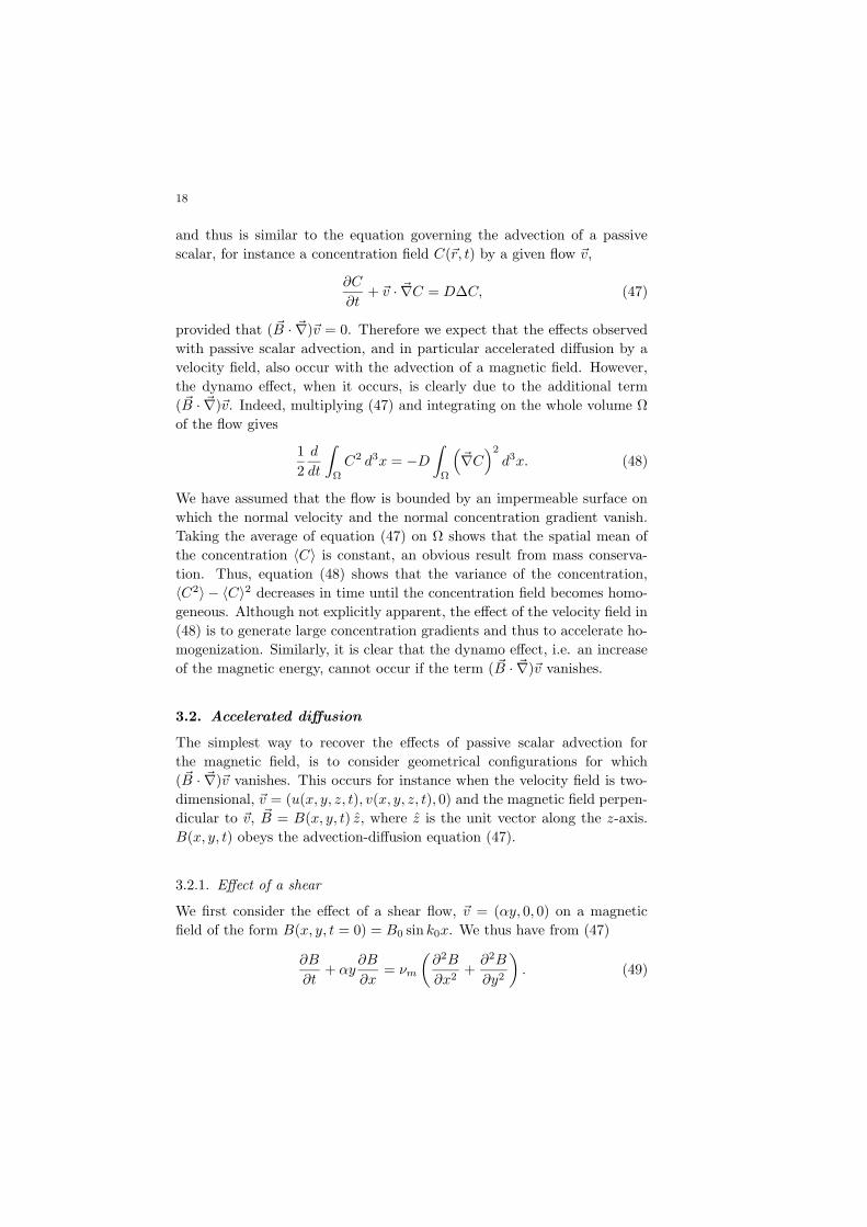
3.2.1. Effect of a shear

We first consider the effect of a shear flow, ~v = (αy, 0, 0) on a magnetic

field of the form B(x, y, t = 0) = B0 sin k0x. We thus have from (47)

∂B

∂t+ αy

∂B

∂x= νm

(

∂2B

∂x2+∂2B

∂y2

)

. (49)

19

In the limit of infinite conductivity, νm = 0, the field is just advected by

the flow

Badv = B0 sin k0(x− αyt). (50)

For finite νm, we look for a solution in the form B(x, y, t) = f(t)Badv and

get from (49)

f = −νmk20(1 + α2t2)f. (51)

We thus have

B(x, y, t) = B0 sin k0(x− αyt) exp

(

−νmk20(t+α2

3t3)

)

. (52)

With equation (48) in mind, we compute 〈(~∇B)2〉

〈(~∇B)2〉 = 1

2B20k

20

(

1 + α2t2)

exp

(

−2νmk20(t+α2

3t3)

)

. (53)

〈(~∇B)2〉 begins to increase as in the case without diffusion. When large

enough gradients have been generated by the advection of the magnetic

field by the shear flow, Joule dissipation becomes important and 〈(~∇B)2〉decreases to 0. For νm small, the characteristic time for which 〈(~∇B)2〉begins to decrease is

τshear ∝(

νmk20α2)− 1

3 . (54)

τshear is the effective diffusion time by the shear flow and should be com-

pared to the diffusion time in the absence of flow τd = (νmk20)−1 which is

much longer if νm is small.

3.2.2. Effect of a strain

We now consider the effect of a flow with a uniform rate of strain, ~v =

(αx,−αy, 0). We have to solve

∂B

∂t+ αx

∂B

∂x− αy

∂B

∂y= νm

(

∂2B

∂x2+∂2B

∂y2

)

. (55)

We look for a solution of the form B(x, y, t) = B0f(t) sin k(t)x and get 7

k(t) = k0 e−αt, (56)

B(x, y, t) = B0 exp

[

νmk20

2α

(

e−2αt − 1)

)

]

sin k(t)x. (57)

20

If α < 0, the flow generates large gradients of B and this strongly increases

Joule dissipation, thus leading to an effective diffusion time

τstrain ∝1

αLog

(

α

νmk20

)

. (58)

For νm small, τstrain is much smaller than τshear, thus showing that mixing

is more efficient than with a shear flow. This is clearly due to the fact

that large gradients are generated more quickly within the regions of large

strain.

3.3. Local amplification

Another simple configuration consists of a magnetic field, ~B =

(Bx(x, y, t), By(x, y, t), 0), in the plane of a two-dimensional flow, ~v =

(vx(x, y, t), vy(x, y, t), 0). It is convenient to consider the equation gov-

erning the vector potential ~A with ~B = ~∇ × ~A. We get from equation

(45)

∂ ~A

∂t= ~v ×

(

~∇× ~A)

− ~∇φ+ νm∆ ~A, (59)

where φ(x, y, z, t) is the scalar potential.

For a two-dimensional magnetic field, ~B = ~∇ × (Az) = ~∇A × z =

(∂A/∂y,−∂A/∂x, 0), we have

∂A

∂t+ ~v · ~∇A = νm∆A, (60)

thus A obeys an advection-diffusion equation. Consequently, we do not

expect new effects compared to the passive scalar advection. However, it

is interesting to discuss some consequences of equation (60) in terms of the

magnetic field.

3.3.1. Effect of a shear

We first consider the effect of a shear flow ~v = (αy, 0, 0) on an externally

applied transverse magnetic field ~B0 = (0, B0, 0). The equation governing

the vector potential Az is

∂A

∂t+ αy

∂A

∂x= νm∆A. (61)

If we consider the behavior of the magnetic field on a short time scale

after turning on the flow, we can neglect diffusion and we get the solution,

A(x, y, t) = −B0(x − αyt), thus ~B = (B0αt,B0, 0). We thus observe that

a magnetic field along the axis of the shear is induced. We look for a

21

stationary solution of equation (61) in the form A(x, y) = −B0x + f(y)

and get for the magnetic field ~B =(

B0αy2/2νm, B0, 0

)

. The solution goes

to infinity because the applied magnetic field and the velocity field both

extend to infinity.

If we consider a localized jet around the x-axis, of the form ~v =(

v0/ cosh2 ky, 0, 0

)

, we get ~B = (−B0Rm tanh ky,B0, 0), where Rm =

v0/kνm. The induced field is constant for y → ±∞ because the jet is

infinite along the x-axis. We thus find that at large Rm, the magnetic field

tends to become aligned with the shear flow. This can be understood very

easily by looking at the current induced by the interaction of the externally

applied magnetic field with the velocity field.

3.3.2. Effect of a strain

We next consider the effect of a flow with a uniform rate of strain, ~v =

(αx,−αy, 0), on a magnetic field along the x-axis, and thus depending only

on y and t (α > 0). We have to solve

∂A

∂t− αy

∂A

∂y= νm

∂2A

∂y2. (62)

We thus get for the stationary solution of the magnetic field, ~B =

B0 exp(

−αy2/2νm)

x. This solution is similar to the one of the Burgers

vortex for vorticity amplified by strain. The magnetic field is concentrated

on a typical length scale√

νm/α. A magnetic tube of length l along the

x-axis becomes elongated along x and thus thinner along y, when it is ad-

vected toward the x-axis; thus the magnetic field is amplified in order to

have flux conservation. We can indeed check that the total magnetic flux is

conserved 7. Let us emphasize that we do not have here any dynamo effect

but just local amplification of an existing magnetic field by the flow.

3.4. Expulsion of a transverse magnetic field from a

rotating eddy

We study the effect of a rotating eddy on a transverse magnetic field~B0 = B0 y as sketched in Figure 3. The eddy of radius R is infinite in

the axial direction x and rotates at an angular velocity ω. The results do

not depend on the electrical conductivity of the external medium (conduc-

tor or insulating).

Writing ~B = ~B0 +~b, the stationary induced magnetic field is solution

of the equation

νm∆~b+∇× (~v ×~b) = −∇× (~v × ~B0) . (63)

22

R 0 x

y

z

z

x yθ

ur

B0

ω

Figure 3. Rotating eddy submitted to a transverse magnetic field.

In the limit of low velocity, b¿ B0 and we have to solve

νm∆~b ≈ −∇× (~v × ~B0) . (64)

Using cylindrical coordinates (r = cos θy + sin θz), we obtain for r ≤ R

br = −B0 ωR

2

8 νm

(

( r

R

)2

− 2

)

sin θ ,

bθ =B0 ωR

2

8 νm

(

2− 3( r

R

)2)

cos θ ,

bx = 0 . (65)

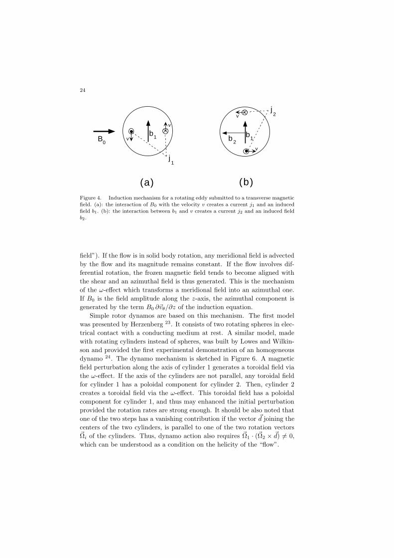
This field is generated by the interaction between the rotating eddy and

the applied magnetic field ~B0 which creates a current ~j1 and a magnetic

field ~b1 as sketched in Figure (4 a). With the description of this “one-step”

mechanism, one can understand the linear dependence of the field in ω.

At higher velocity, terms of higher order must be taken into account.

The solution of equation (63) is given in terms of the Bessel function

I(n, x) 21

br = B0Re

(

(I(0, q r)

I(0, q R)− I(2, q r)

I(0, q R)− 1) exp (i θ)

)

,

bθ = B0Re

(

(I(2, q r)

I(0, q R)+

I(0, q r)

I(0, q R)− 1) exp (i (θ + π/2))

)

,

bx = 0 , (66)

23

where q = exp(iπ/4)√

ωνm

. Expanding this result in successive powers of

the angular velocity gives

br =−B0 ωR

2

8 νm

(

( r

R

)2

− 2

)

sin θ

+B0 ω

2R4

ν2m

(

−(

rR

)4

192+

(

rR

)2

32− 3

64

)

cos θ ,

bθ =B0 ωR

2

8 νm

(

2− 3( r

R

)2)

cos θ

− B0 ω2R4

ν2m

(

5(

rR

)4

192− 3

(

rR

)2

32+

3

64

)

sin θ ,

bx =0 . (67)

The term linear in ω is the one previously calculated. The quadratic term

results from the interaction of the induced magnetic field b1 with the ve-

locity field as sketched in Figure (4 b). In that sense, this is a “two-step”

mechanism and since b1 is linear in ω, b2 is quadratic.

These are the first steps of the mechanism of expulsion of the transverse

magnetic field. At very high velocity, the field enters the eddy only in a

small diffusive layer of length√

νm/ω. This corresponds to the usual skin

effect as can be understood in the frame of the rotating eddy where the

applied magnetic field is oscillatory.

In the case of a liquid metal in rotation in a cylindrical container, the

velocity field vanishes at the boundaries and solid body rotation is thus

achieved only in the bulk. Then, a transverse magnetic field is expelled

from the bulk but becomes more intense near the boundaries as shown by

experiments made in liquid gallium 22.

3.5. Effect of differential rotation and the Herzenberg

dynamo

We have already shown that a shear flow generates a magnetic field com-

ponent parallel to the shear from a perpendicularly applied one. In other

words, field lines tend to become aligned along the shear and the field

amplitude is enhanced if the shear is strong enough. In geophysical and as-

trophysical fluid dynamics, very common flows with shear are axisymmetric

flows which involve differential rotation. For such flows, a toroidal field is

generated from an applied poloidal one. This effect is called the ω-effect

and is very similar to the effect of a shear presented above. We sketch

this mechanism in Figure 5 in the limit of zero magnetic viscosity (“frozen

24

B0

1j

b1

2j

b1b

2

(a) (b)

v

v

v

v

Figure 4. Induction mechanism for a rotating eddy submitted to a transverse magnetic

field. (a): the interaction of B0 with the velocity v creates a current j1 and an induced

field b1. (b): the interaction between b1 and v creates a current j2 and an induced fieldb2.

field”). If the flow is in solid body rotation, any meridional field is advected

by the flow and its magnitude remains constant. If the flow involves dif-

ferential rotation, the frozen magnetic field tends to become aligned with

the shear and an azimuthal field is thus generated. This is the mechanism

of the ω-effect which transforms a meridional field into an azimuthal one.

If B0 is the field amplitude along the z-axis, the azimuthal component is

generated by the term B0 ∂~vθ/∂z of the induction equation.

Simple rotor dynamos are based on this mechanism. The first model

was presented by Herzenberg 23. It consists of two rotating spheres in elec-

trical contact with a conducting medium at rest. A similar model, made

with rotating cylinders instead of spheres, was built by Lowes and Wilkin-

son and provided the first experimental demonstration of an homogeneous

dynamo 24. The dynamo mechanism is sketched in Figure 6. A magnetic

field perturbation along the axis of cylinder 1 generates a toroidal field via

the ω-effect. If the axis of the cylinders are not parallel, any toroidal field

for cylinder 1 has a poloidal component for cylinder 2. Then, cylinder 2

creates a toroidal field via the ω-effect. This toroidal field has a poloidal

component for cylinder 1, and thus may enhanced the initial perturbation

provided the rotation rates are strong enough. It should be also noted that

one of the two steps has a vanishing contribution if the vector ~d joining the

centers of the two cylinders, is parallel to one of the two rotation vectors~Ωi of the cylinders. Thus, dynamo action also requires ~Ω1 · (~Ω2 × ~d) 6= 0,

which can be understood as a condition on the helicity of the “flow”.

25

a) solid body rotation b) differential rotation

B0

B0

bθ

Figure 5. (a) A magnetic field frozen in the fluid is advected without being modified

by solid body rotation. (b) In the case of differential rotation, the field lines becomealigned with the shear. This generates an azimuthal field component.

4. Necessary conditions for dynamo action

We will consider the equation governing the magnetic energy and use it

to find necessary conditions for an increase of the magnetic energy from

mechanical work. In particular we will discuss the importance of the flow

geometry and review some configurations for which the dynamo action does

not occur.

4.1. Magnetic energy

We consider the flow of an electrically conducting fluid in a volume Ω

inside a surface S surrounded by a motionless insulator occupying the rest

of space. We assume that there are no sources of field outside Ω, thus

E = O(r−2), B = O(r−3) as r →∞. (68)

From equation (9), we get for the evolution of the magnetic energy, EM ,

dEM

dt=

d

dt

∫

B2

2µ0d3x =

∫ ~B

µ0

∂ ~B

∂td3x = −

∫ ~B

µ0~∇× ~E d3x. (69)

Using ~∇ · ( ~B × ~E) = − ~B · (~∇× ~E) + ~E · (~∇× ~B) and taking into account

that | ~E × ~B| = O(r−5) as r → ∞ such that we have no contribution from

26

omega effect

omega effect

Ω1

Ω2

Figure 6. Rotating cylinders in electrical contact with an electrically conducting

medium at rest. The toroidal field of each cylinder has a non-zero component alongthe axis of the other one. Thus each toroidal field may be generated by the other one

through the ω-effect.

its surface integral, we get

dEM

dt= −

∫

Ω

~E ·~j d3x. (70)

Then, Ohm’s law (15) gives

dEM

dt=

∫

Ω

(~v × ~B) ·~j d3x−∫

Ω

~j2

σd3x. (71)

The last term of equation (71) represents Joule dissipation, whereas the

first term of the right hand side describes energy transfer from the velocity

field and may lead to an increase of the magnetic energy if it overcomes

Joule dissipation.

27

Using the Cauchy-Schwarz inequality, we obtain∣

∣

∣

∣

∫

Ω

~v · ( ~B × (~∇× ~B))d3x

∣

∣

∣

∣

≤ VM

∫

Ω

| ~B||~∇× ~B| d3x

≤ VM

[∫

B2 d3x

]12[∫

Ω

(~∇× ~B)2d3x

]12

(72)

where VM is the maximum of |~v| on Ω. Defining

1

H2≡ min

[

∫

Ω(~∇× ~B)2 d3x∫

B2 d3x

]

, (73)

where the minimum is taken on all possible admissible magnetic fields

(solenoidal, irrotational outside Ω, O(r−3) at infinity and satisfying the

appropriate boundary conditions on S), we get

dEM

dt≤ 1

µ20σ(µ0σVMH − 1)

∫

Ω

(~∇× ~B)2 d3x. (74)

A necessary condition for dynamo action is thus 2

µ0σVMH ≥ 1. (75)

A second condition can be obtained if the flow is incompressible. Using~B × (~∇× ~B) = ~∇(B2/2)− ( ~B · ~∇) ~B, we obtain∫

Ω

~v · ( ~B × (~∇× ~B)) d3x =

∫

S

B2

2~v · ndS −

∫

Ω

~v · ( ~B · ~∇) ~B d3x. (76)

On the right hand side, the incompressibility condition and the divergence

theorem have been used to transform the first term which vanishes because

~v = 0 on S. Using ~∇ · ~B = 0 and integrating by parts, we have for the

second term in tensor notations∫

Ω

viBj∂jBi d3x =

∫

Ω

vi∂j(BiBj) d3x

=

∫

S

BiBjvinjdS −∫

Ω

BiBj∂jvi d3x, (77)

where the surface integral again vanishes because ~v = 0 on S. Thus,

dEM

dt=

1

2µ0

∫

Ω

BiBj (∂jvi + ∂ivj) d3x−

∫

Ω

~j2

σd3x, (78)

that can be also found directly by multiplying equation (46) by ~B and in-

tegrating over space. It is interesting to compare this second form of the

evolution equation for the magnetic energy to the first one (71). In (78), the

term describing energy transfer from the velocity field is quadratic in Bi and

28

involves the derivatives of the velocity field whereas in (71) it involves the

velocity field itself times the magnetic field and its space derivatives. Con-

sequently, a second necessary condition for dynamo action can be obtained

from (78). Let ΛM be the maximum eigenvalue of the tensor (∂jvi+∂ivj)/2

(ΛM > 0 for non vanishing velocity fields). We have

1

2

∫

Ω

BiBj (∂jvi + ∂ivj) d3x ≤ ΛM

∫

B2 d3x

≤ ΛMH2

∫

Ω

(~∇× ~B)2 d3x, (79)

and consequently

dEM

dt≤ 1

µ20σ(µ0σΛMH2 − 1)

∫

Ω

(~∇× ~B)2 d3x. (80)

A second necessary condition for dynamo action is thus 25

µ0σΛMH2 ≥ 1. (81)

4.2. The critical magnetic Reynolds number

The above necessary conditions imply that for µ0σ fixed, H, ΛM and VMshould be large enough. The condition on H is easy to understand. H is the

typical lengthscale related to the magnetic field gradients and should be as

large as possible in order to minimize Joule dissipation. It is less obvious to

understand why we have apparently two independent constraints to make

the dynamo capability of the term ~∇×(~v× ~B) in equation (45) large enough:

ΛM large or VM large. Are they independent ? At first sight, ΛM is related

to the flow gradients whereas VM is an absolute velocity magnitude. This is

not completely correct because equation (45) is invariant in reference frames

translating or rotating at constant velocity one from each other. Since the

necessary condition (75) can be obtained in any of them, VM should be

understood as a velocity difference with respect to any uniform velocity (in

an unbounded domain) or to any velocity field corresponding to solid body

rotation. We may relate VM and ΛM by defining the scale l ≡ VM/ΛM . l

is a characteristic scale related to velocity gradients. The problem is thus

to determine whether H and l are independent or not. On one side, the

magnetic field being generated by the velocity field, one may expect that H

depends on l. On the other side, it is unlikely that H depends uniquely on l;

it certainly depends on the flow geometry as can be seen by considering the

form of the term responsible for possible dynamo action in (74) and (80).

Then, it may be possible to vary H and l independently by tuning some

29

appropriate flow parameter. Thus, one have to locate the region where

dynamo action is impossible in a two-parameter space, (Rm, L/l) displayed

in Fig. 7 where Rm ≡ µ0σLVM .

The main difficulty is that the necessary conditions (75,81) involve the

parameters H and ΛM that are not directly controlled in an experiment.

The above discussion illustrates that Rm is not the only relevant dimension-

less parameter to describe dynamo onset. Indeed, the conditions (75,81)

are not sufficient for dynamo action. We will discuss below examples of

“antidynamo theorems” which show that dynamo action is impossible for

particular geometries of the velocity and/or the magnetic fields.

Rm

L / l1

L H/

Figure 7. The necessary conditions (75,81) correspond to Rm > L/H and Rm >

Ll/H2. Dynamo action is not possible outside the shaded region.

4.3. “Antidynamo theorems”

It has been first shown by Cowling in 1934 26 that an axisymmetric magnetic

field cannot be maintained by dynamo action. Several such “anti-dynamo

theorems” have been found since. They state that either magnetic fields

of given geometries cannot be generated by a fluid dynamo or that flows

of given geometries cannot undergo a dynamo instability. Cowling’s result

belongs to the first class. It should be emphasized that it does not con-

cern the problem of the dynamo capability of an axisymmetric flow. An

axisymmetric flow may indeed generate a non axisymmetric magnetic field

(see the section on laminar dynamos). On the contrary, it is known that,

30

two-dimensional flows i.e. with velocity fields with one vanishing compo-

nent in cartesian coordinates 27, toroidal flows i.e. flows with a vanishing

radial component in spherical geometry 28,25 do not lead to dynamo ac-

tion. Most of these results have been extended to compressible flows and

it has been also shown that a purely radial flow in spherical geometry can-

not sustain a magnetic field 29. Note however that a flow without radial

component can generate a magnetic field in cylindrical geometry (see the

section about laminar dynamos). It should be stressed that most of these

results have not been demonstrated with all possible boundary conditions.

Several demonstrations are also restricted to time independent magnetic

fields which is clearly a too strong assumption. We will not give here the

demonstrations of all the above results. For a review from a mathematical

view point, we refer to Nunez 30.

5. Laminar dynamos

There exist very few laminar flows for which dynamo action can be shown

analytically. This is partly due to “antidynamo theorems” that rule out

many simple flows. Examples of analytically tractable dynamos are of

great interest to understand the basic mechanisms that give rise to dy-

namo action. So one can get an idea about the flow properties responsible

for its good dynamo capability. The kinematic dynamo problem is solved

numerically in most cases. It should be noted that it is much more sensi-

tive to truncation errors than most of the other hydrodynamic instabilities.

Several examples of dynamos obtained in the past indeed resulted from a

lack of numerical resolution or equivalently because a too small number

of modes was kept. This extreme sensitivity with respect to resolution is

certainly related to the geometry of the neutral magnetic modes which are

often strongly localized in space.

We have already mentioned the rotor dynamo of Herzenberg 23 and its

experimental demonstration by Lowes and Wilkinson 24. Although these

flows give rise to homogeneous dynamos, they may look somewhat artificial

since the fact that they are not simply connected in space is an essential

feature. A laminar flow in a simply connected domain displaying dynamo

action was found by Lortz 31 but without any illustrative example. We

will first consider in this section the Ponomarenko dynamo 32 which is

driven by a very simple helical flow. This flow as well as other helical flows

with more realistic velocity profiles are known to have the best dynamo

capability among all the known laminar dynamos. We will next consider

another class of flows for which the magnetic field is generated at a scale

large compared to the one of the flow. This occurs for many spatially

31

periodic flows as shown by G. O. Roberts 33,34 and makes the analysis

much simpler. Finally, we will make some comments related to the nature

of the bifurcation corresponding to the dynamo onset (broken symmetries,

Hopf or stationary bifurcation, etc).

5.1. The Ponomarenko dynamo

5.1.1. Linear stability analysis

The Ponomarenko dynamo consists of a cylinder of radius R, in solid body

rotation at angular velocity ω, and translation along its axis at speed V ,

embedded in an infinite static medium of the same conductivity with which

it is in perfect electrical contact (Figure 8). Using respectively, R, µ0σR2,

(µ0σR)−1, as units for length, time and velocity, the governing equation

for the magnetic field, ~B(~r, t), is

∂ ~B

∂t= ∇× (~v × ~B) +∇2 ~B . (82)

The kinematic dynamo problem, i.e. the linear stability analysis of the

solution B = 0 of (82), is governed by two dimensionless numbers

Rm = µ0σR√

(Rω)2 + V 2, Ro =V

Rω. (83)

The dimensionless velocity field is

~v =

0

rRm/√1 +Ro2

Rm/√1 +Ro−2

for r < 1 (84)

and vanishes for r > 1. The neutral modes are of the form

~B(~r, t) = ~bp(r) exp i(ω0t+mθ + kz). (85)

We have a Hopf bifurcation if ω0 6= 0 and a stationary bifurcation otherwise.

We write equation (82) in the form

L~B ≡ ∂ ~B

∂t−∇× (~v × ~B)−∇2 ~B = 0, (86)

and get for magnetic fields of the form (85)

Lr ~bp ≡ i(ω0 + µΓ(r))~bp −∆~bp +Dl~bp = 0 , (87)

where µ = (µ0σR2)(mω + kv) and Γ(r) = 1 for r < 1 and Γ(r) = 0 for

r > 1.

32

ω

v

R

helical

flow

conducting medium at rest

Figure 8. Sketch of the Ponomarenko dynamo.

The operator ∆ traces back to Joule dissipation in the induction equa-

tion,

∆ =

l.− 1r2 − 2imr2 0

2imr2 l.− 1

r2 0

0 0 l.

, (88)

where l is an operator defined by

l.f =1

r

d

dr

(

rdf

dr

)

− (m2

r2+ k2)f . (89)

Note that the non diagonal terms of ∆ couple the radial and azimuthal

components of the magnetic field. The coupling vanishes if m = 0 for

which dynamo action is impossible in agreement with Cowling anti-dynamo

theorem (the magnetic field being axisymmetric). We emphasize that this

coupling, essential for dynamo action, results from Joule dissipation, and

governs the large Rm behavior of the Ponomarenko dynamo. It could be

understood as an “α-effect” (see below).

Dl results from the velocity discontinuity for r = 1. Its expression,

Dl =

0 0 0

Rωδ(r − 1) 0 0

V δ(r − 1) 0 0

, (90)

shows how the shear at r = 1 generates the azimuthal and axial components

of the field from the radial one. As explained in the section on advection

and diffusion of a passive vector, the magnetic field tends to become aligned

with the shear flow. This can be also understood as an “ω-effect”. The

discontinuity of the derivatives of the θ and z-components of the magnetic

field at r = 1 is thus proportional to the value of Br.

Thus, we can understand qualitatively the mechanism of Ponomarenko

dynamo: a perturbation Br gives rise to Bθ and Bz under the action of the

33

shearing motion along θ and z at r = 1. Br is then regenerated by Joule

diffusion of Bθ provided that m 6= 0. We note that this mechanism subsists

for more realistic helical flows without a discontinuity for r = 1. Smoothing

the discontinuity thus creating a region of width δ with strong shear in

the vicinity of r = 1, does not affect qualitatively the above mechanism;

only the limit Rm → ∞ or any other limit involving spatial scales small

compared to δ may be affected.

The dynamo threshold can be found by solving equation (87) for r < 1

and r > 1 and then writing boundary conditions at r = 1. We first note

that we have only to find br et bθ. Indeed, ~B being solenoidal,

1

r

d(rbr)

dr+im

rbθ + ikbz = 0 . (91)

Defining b± = br ± ibθ, we get

1

r

d

dr

(

rdb±dr

)

−(

(m± 1)2

r2+ (k2 + p+ iµΓ(r))

)

b± = 0. (92)

b± are thus decoupled for r < 1 and r > 1 and the solutions are given by

the Bessel functions I(n, x) et K(n, x) 21. In order to avoid divergence of

the solutions for r = 0 and r →∞, we take

r ≤ 1 b± = A±I(m±1,qr)I(m±1,q) with q2 = p+ k2 + iµ , (93)

r ≥ 1 b± = B±K(m±1,sr)K(m±1,s) with s2 = p+ k2 . (94)

The four unknowns, A± et B± are determined by boundary conditions at

r = 1. The normal component of ~B and the tangential components of ~H

and therefore of ~B being continuous, b± should be continuous and thus,

A± = B±. The continuity of ~B and (91) imply that dbr/dr is continuous.

Finally, the continuity of the tangential component of the electric field

implies that dbθ/dr+ vθbr is continuous. We thus have four unknowns and

four conditions. The existence of non trivial solutions for A± requires

R+R− =iω

2(R+ −R−) , (95)

where

R± = qI ′(m± 1, q)

I(m± 1, q)− s

K ′(m± 1, s)

K(m± 1, s). (96)

The numerical resolution of this equation gives the growth rate p =

Φ(Rm, Ro, k,m) where Φ is a function of the parameters Rm, Ro, k,m. At

the instability onset, Re(p) = 0 gives the critical magnetic Reynolds num-

ber for dynamo action Rmc = Ψ(Ro, k,m). The minimum corresponds to

m = 1, Ro = 1.314, k = kc = −0.38, for which we have Rmc = 17.72 and

34

ω0 = 0.410. We thus have a Hopf bifurcation. m = 0 is impossible from

Cowling’s anti-dynamo theorem and m larger than 1 leads to an increased

Joule dissipation. We note that the maximum dynamo capability of the

flow (Rmc minimum) is obtained when the azimuthal and axial velocities

are of the same order of magnitude (Ro ∼ 1). This trend is often observed

with more complex flows for which the maximum dynamo capability is ob-

tained when the poloidal and toroidal flow components are comparable.

Finally, note that the pitches of the helices of the magnetic field and of the

velocity field are opposite but not equal in magnitude such that µ 6= 0. The

magnetic field becomes more and more aligned with the shear at large Rm

and the kinematic problem is easier to solve for modes with a wavelength

small compared to R 3,35,36 . We show next that the dynamo onset occurs

in a high Rm limit when Ro→ 0, which makes its study simpler.

0 1 2 3 4 5 6 7 80

0.2

0.4

0.6

0.8

1

1.2

1.4

1.6

1.8

2

r

br

bθ

bz

Figure 9. Absolute value of the components of the unstable mode of the Ponomarenkodynamo.

35

5.1.2. The high rotation rate limit

Although Rmc tends to infinity, the linear stability analysis becomes simpler

in the limit of high rotation rate, Ro → 0. The field is mostly sheared in

the azimuthal direction and thus kc → ∞. The argument of the Bessel

functions then tends to infinity and it is possible to use their asymptotic

expressions. We thus obtain

Rmc = 4√2Ro−3 , (97)

ωo =√3Ro−2 , (98)

kc = −Ro−1 , (99)

µ¿ ωo . (100)

Rmc tends to infinity because the flow becomes two dimensional in the limit

Ro→ 0, for which dynamo action becomes impossible. Note however that

the wavelength of the neutral mode vanishes proportionally to Ro. Thus,

at the spatial scale of the neutral mode, the flow remains three-dimensional

and dynamo action remains possible for any value of Ro. This last result

may be modified if the velocity discontinuity is smoothed.

The validity of our asymptotic calculation is checked by comparing the

above results to the ones obtained by numerically solving the full problem

(Figure 10). The agreement is good even for Ro ∼ 1.

The expressions for the fields are also simpler in the high rotation rate

limit. Writing q =√2eiπ/6Ro−1, we get for r ≤ 1

br =1

2(I(2, qr)

I(2, q)− I(0, qr)

I(0, q))− 1

q2I(0, qr)

I(0, q),

bθ =1

2i(I(2, qr)

I(2, q)+I(0, qr)

I(0, q)) +

1

iq2I(0, qr)

I(0, q), (101)

and for r ≥ 1

br =1

2(K(2, qr)

K(2, q)− K(0, qr)

K(0, q))− 1

q2K(0, qr)

K(0, q),

bθ =1

2i(K(2, qr)

K(2, q)+K(0, qr)

K(0, q)) +

1

iq2K(0, qr)

K(0, q), (102)

from which bz can be computed using ~∇ · ~B = 0. The field components

are displayed in Figure 11. The field becomes more and more localized

close to r = 1 when Ro → 0. From the qualitative description of the

mechanisms responsible for the Ponomarenko dynamo, Bθ (respectively

Bz) is generated from Br by the velocity shear Rω (respectively V ). Thus,

we expect Bz ∝ RoBθ. Br is regenerated from Bθ, thus Br ∝ Ro2Bθ (from

equations (87, 88) and ω0 ∝ Ro−2).

36

10-2

10-1

100

100

101

102

103

104

105

106

107

Rmc

R o10

-210

-110

010

-1

100

101

102

103

104

105

ω0

R o

Figure 10. Critical magnetic Reynolds number Rmc and pulsation at onset ω0 as a

function of the Rossby number Ro. The cross are numerical solutions of equation (95).The full line is the asymptotic solution given by equations (97) and (98).

5.1.3. Further remarks on the Ponomarenko dynamo

As already mentioned, the velocity discontinuity is a rather unrealistic fea-

ture of the Ponomarenko dynamo. If the solid rotor is replaced by the

helical flow of a liquid metal, the velocity field then becomes of the form

~v = (0, vθ(r), vz(r)) and should vanish for r = 1. The corresponding

kinematic dynamo problem has been studied theoretically 35,36 and self-

generation of the magnetic field has been observed experimentally (Riga

experiment) 37. Although this decreases the value of Rmc, the presence of

an external conducting medium is not required any more when the velocity

profile depends on r. In the case of solid body rotation and translation,

the presence of a conducting external medium is necessary because the dy-

namo problem is unchanged in reference frames rotating and translating at

constant velocity one from each other; thus, the Ponomarenko problem is

unchanged if the rotor is static and the external medium moves at velocity

−V along the z-axis with a rotation rate −ω. With an insulating external

medium, this motion obviously cannot drive any dynamo. The dynamo

capability of helical flows remains almost unchanged with realistic velocity

37

0.5 0.6 0.7 0.8 0.9 1 1. 1 1. 2 1. 3 1. 4 1. 50

0.2

0.4

0.6

0.8Ro -2

b r

r

0.5 0.6 0.7 0.8 0.9 1 1. 1 1. 2 1. 3 1. 4 1. 50

0.5

1

1. 5

b θ

r

0.5 0.6 0.7 0.8 0.9 1 1. 1 1. 2 1. 3 1. 4 1. 50

0.5

1

1. 5

Ro -1 bz

r

Figure 11. Absolute value of the components of the unstable mode of the Ponomarenkodynamo in the small Rossby number limit: Ro−1 = 15 (dotted lines), Ro−1 = 30 (dash-dotted lines), Ro−1 = 45 (full lines).

profiles. Indeed, a critical magnetic Reynolds number of order 20 has been

observed in the experiments 37. On the contrary, the behavior of the growth

rate for Rm →∞ strongly depends on the flow profile. With a smooth heli-

cal flow, the growth rate decreases to zero when Rm →∞ whereas it tends

to a finite value in the case of the Ponomarenko dynamo 36. With a smooth

flow, the regeneration of Br from Bθ vanishes in the limit Rm →∞ because

it is due to Joule dissipation. This does not occur with the discontinuous

profile because the most unstable wavenumber can increase with Rm thus

keeping the effect of Joule dissipation constant in the limit Rm →∞.

5.2. Spatially periodic dynamos

It has been shown by G. O. Roberts 33,34 that many spatially periodic

flows generate a magnetic field at a large scale compared to their spatial

periodicity. After discussing the importance of this scale separation, we

present two examples of such flows.

38

5.2.1. Scale separation

We have already mentioned that the term ( ~B · ~∇)~v is the main source term

for the amplification of the magnetic field which is dissipated by the diffusive

term νm∇2 ~B. Thus, self-generation of a large scale magnetic field looks

easier because Joule dissipation per unit volume vanishes if the wavelength

of the field tends to infinity. This has obviously some cost since it requires

to drive a flow in a very large domain. If the magnetic field is generated on

spatial scale L, large compared to the one of the velocity field, l, we may

define the magnetic Reynolds number as usual with the ratio of the above

two terms and get: Rm1 = µ0σV L2/l = PmRe(L/l)

2, where Pm = µ0σν is

the magnetic Prandtl number and Re = V l/ν is the Reynolds number of the

flow. This definition is strongly misleading because it gives the impression

that increasing scale separation, i.e. increasing L/l, may be as efficient as

increasing µ0σ or the flow velocity to get dynamo action. This is of course

not true in general. There are three independent dimensionless parameters

in the problem, Rm1, Re, L/l or alternatively, Rm1, Pm, L/l. The critical

magnetic Reynolds number is thus of the form

Rcm1 = f(Pm, L/l) , (103)

where f is an arbitrary function at this stage. The dependence on Pmmeans that the dynamo capability of the flow may depend on its level of

turbulence (see next section). The dependence on L/l determines whether

scale separation is good for dynamo action. This of course depends on the

criterion we choose: let us first take a minimum kinetic Reynolds number

for a given fluid. Assuming a dependence of the form (L/l)n, one should

have n < 2 in order to take profit from scale separation. It is likely that

n > 0 because the large scale magnetic field cannot be generated without

a small scale component driven by the interaction of the small scale flow

with the large scale magnetic field. The resulting small scale magnetic field

leads to an increased dissipation and thus to a larger value of Rcm1. It is

even likely that n > 1, otherwise it will be possible to generate a dynamo

for fixed L just by taking the limit l→ 0, some sort of “microdynamo” !

We consider a spatially periodic velocity field with wavelength l and

assume that a magnetic field ~B0 is generated on a spatial scale L. As said

above, a field with spatial periodicity l is generated by the interaction of~B0 with the flow. We thus write

~B = ~B0 +~b , (104)

with 〈~b〉 = 0 where 〈·〉 stands for the spatial average on one wavelength l.

Inserting (104) in the induction equation, and averaging over space, we get

39

the evolution equation for the mean field ~B0

∂ ~B0∂t

= ~∇× 〈~v ×~b〉+ νm∆ ~B0. (105)

Subtracting (105) from the induction equation, we get the evolution equa-

tion for the fluctuating field ~b

∂~b

∂t= ~∇×

(

~v × ~B0 + ~v ×~b− 〈~v ×~b〉)

+ νm∆~b. (106)

We have to find ~b as a function of ~B0 using equation (106) in order to get

a closed equation for the mean field from (105). (106) may be solved easily

if ~b is small compared to ~B0; we then have at leading order a diffusion

equation for ~b with a source term depending on ~B0 and the velocity field.

Then, we get

νmb

l2∼ vB0

l, thus b ∼ vl

νmB0. (107)

Using this expression of b in order to estimate 〈~v × ~b〉 which does not

depend any more on l after being averaged, we get from (105) the following

condition for dynamo onset

v2c l

νm

B0L∼ νmB0

L2, thus vc ∼

νm√Ll. (108)

We first observe that b ∼√lLB 0¿ B0 provided that l¿ L. We have for the

Reynolds number of the flow Re ∼√

lL P

−1m ¿ 1 if Pm is not too small.

The magnetic Reynolds number at dynamo onset is Rcm1 = µ0σvcL

2/l ∼(L/l)3/2 À 1, thus n = 3/2. We observe that the relevant definition here

for the magnetic Reynolds number would be

Rm2 ≡ µ0σv√Ll, (109)

the critical value of which for dynamo onset is Rm2 ∼ 1. Consequently,

even if the above mechanism works, we cannot reach the dynamo onset

just by increasing scale separation. For νm and v fixed, it does not help

to decrease l. Whether scale separation makes easier the experimental

observation of the dynamo effect still deserves more discussion (see next

section). At this stage, scale separation makes possible to keep the kinetic

Reynolds number small at dynamo onset. However, with a realistic value

of Pm (Pm ∼ 10−5), one needs an enormous scale separation. With Pm of

order 1, the critical magnetic Reynolds number is small if it is defined with

l only but is of order√

L/l À 1 if it is defined with L only. The main

advantage of scale separation is that it makes analytical calculations much

40

easier. This is a general feature of long wavelength instabilities associated

with hydrodynamic modes, i.e. modes with vanishing growth rate at zero

wavenumber 38. We will illustrate this below.

5.2.2. The G. O. Roberts’ dynamo

We consider the spatially periodic flow of velocity field

~v(x, y, z) =

U sin ky

U cos kx

V (sin kx+ cos ky)

. (110)

We have 〈~v〉 = 0 and the mean helicity is h = 〈~v · ~∇ × ~v〉 = −2kUV .

Assuming that b is small compared to B0, we get from equation (106)

~b ≈ 1

νmk

UB2 cos ky

−UB1 sin kxV B1 cos kx− V B2 sin ky

, (111)

where ~B0 = (B1, B2, B3). We thus get

〈~v ×~b〉 ≈ UV

νmk

1 0 0

0 1 0

0 0 0

~B0 . (112)

We observe that if a large scale field exists along the x or y-axis, the co-

operative effect of small scale periodic fluctuations is to drive a current

parallel to the large scale field. This has been understood by Parker 39

and is due to the helical nature of the flow. Any field B1 along the x-axis

is distorted in the vertical plane x − z by the z-component of the flow of

amplitude V . The field is twisted out of the x − z plane by the toroidal

component of the flow of amplitude U . This drives field loops in the y − z

plane, i.e. a current parallel to x, which generates a magnetic field with

a non-zero component along the y-axis, B2. B2 can then regenerate B1through the same process. The mean electromotive force 〈~v × ~b〉 in the

mean field equation (105) was described by Steenbeck and Krause in 1966

as the “α-effect” (see for instance 8). In this terminology, G. O. Roberts’

dynamo is an α2-dynamo. Defining α = UV/νmk, we have for a mean field

of the form ~B0(Z, T ) = (B1, B2, 0),

∂B1∂T

= −α∂B2∂Z

+ νm∂2B1∂Z2

, (113)

∂B2∂T

= α∂B1∂Z

+ νm∂2B2∂Z2

, (114)

41

Defining A = B1 + iB2, we get

∂A

∂T= −iα∂A

∂Z+ νm

∂2A

∂Z2, (115)

The linear stability analysis of the solution A = 0 (i.e. ~B = 0) is straight-

forward. We consider normal modes of the form A ∝ exp(ηT ± iKZ) and

get from (115) the dispersion relation

η = ±|αK| − νmK2, (116)

which shows that there exists a branch of unstable modes at long enough

wavelength (K < |α|/νm).

We observe that dynamo action vanishes if U → 0 or V → 0 in agree-

ment with antidynamo theorems. It is interesting to consider the behavior

of α when the magnetic Reynolds number becomes larger. To wit, the

calculation of ~b should be performed at higher orders in equation (106).

Solving perturbatively this equation for ~b as an expansion in powers of

U/νmk, one gets

α =UV

νm k

(

1− U2

2 νm2 k2+ ...

)

. (117)

α increases linearly with V but its behavior as a function of U is more

complex. It first increases but reaches a maximum and then decreases as

U is increased. This behavior is due to the expulsion of the transverse

field by the rotating eddies as already shown in 40 by numerically solving

(106). It has been found that α decreases toward zero at large Rm. Note

however that the large Rm limit should be considered carefully. As said

above, the great simplification of scale separation results from the fact that

the magnetic Reynolds number evaluated on the small scale of the flow

is small whereas the one evaluated on the large scale of the mean field is

large. This is clearly apparent in our second order result (117). Truncating

the expansion in U/νm k is not accurate if Rm is too large such that the

magnetic Reynolds number related to the azimuthal motion of the eddies

becomes of order 1.

The α-effect has been demonstrated experimentally by directly mea-

suring the mean electromotive force generated by an helical flow of liquid

sodium submitted to an external magnetic field 41. Self-generation of a

magnetic field by the α-effect has been achieved recently, using a periodic

arrangement of counter-rotating and counter-current helical vortices that

mimic G. O. Roberts’ flow. Axial and azimuthal sodium flows are driven

by pumps in an array of helical ducts immersed in a cylinder (Karlsruhe

experiment) 42.

42

5.2.3. The ABC dynamo

The mean electromotive force 〈~v ×~b〉 can be proportional to ~B0 when the

flow is more symmetric than the one considered above. This can be achieved

with the “ABC” flow

~v(x, y, z) = V

sin ky + cos kz

sin kz + cos kx

sin kx+ cos ky

. (118)

We have 〈~v〉 = 0 and the mean helicity is h = 〈~v · ~∇× ~v〉 = −3kV 2. Using

the same procedure as above, we get

〈~v ×~b〉 ≈ 2V 2

νmk~B0 . (119)

Thus, the mean field ~B0 is governed by the equation

∂ ~B0∂T

= α~∇× ~B0 + νm∆ ~B0. (120)

We consider normal modes of the form ~B0 = B0 exp(ηT ± i ~K · ~R) and get

from (120) the dispersion relation (116).

A mean field equation of the form (120) is expected to leading order for

any small scale flow which is spatially homogeneous and isotropic. Indeed,

for a given velocity field, we expect from equation (106) that ~b is linearly

related to ~B0, thus the mean electromotive force 〈~v ×~b〉 is linearly related

to ~B0. If we assume that, due to scale separation, there exists an expansion

of 〈~v ×~b〉 as a function of ~B0 and its gradients, we get

〈~v ×~b〉i = αi,jB0 j + βi,j,k∂B0 j

∂xk+ · · · , (121)

where the components of the tensors αi,j and βi,j,k are functionals of the

velocity field, i.e. depend on its moments. If the flow is isotropic, αi,j and

βi,j,k should be isotropic tensors, thus αi,j = α δi,j and βi,j,k = β εi,j,k.

Consequently,

〈~v ×~b〉 = α~B0 − β~∇× ~B0 + · · · , (122)

and

∂ ~B0∂T

= α~∇× ~B0 + νt∆ ~B0 , (123)

where νt = νm + β is the “turbulent ” magnetic diffusivity. As said above,

the α-effect is always dominant at large enough scale and leads to dynamo

action provided that α 6= 0. For helical flows, α is proportional to the mean

helicity but it has been shown that a non-zero mean helicity is not necessary

43

for the α-effect 45. However, the flow should not be parity invariant; indeed,

if the flow is symmetric with respect to some plane, α[S.~v] = α[~v] where S

is the corresponding symmetry transformation. On the other side, ~B0 being

a pseudo-vector, it does not transform in the same way as ~∇ × ~B0 under

S. Consequently (123) implies α = 0 and one has to consider the effect of

higher order terms. We have often β > 0, i.e. the magnetic diffusivity is

usually enhanced by the small scale flow but periodic flow configurations

with β < 0 have been also reported 43.

5.2.4. Further remarks on the dynamo bifurcation

- Hopf versus stationary bifurcations

We have studied previously two examples of laminar dynamos generated

by stationary flows: Ponomarenko’s and the G. O. Roberts’ dynamos. The

first one is generated through a Hopf bifurcation, the second is stationary.

Why ? Although general predictions about the nature of the bifurcation

cannot be made, some features can be understood using symmetry consid-

erations 46. Ponomarenko’s flow is invariant under translations along the z

axis z → z + z0 . However, it is not invariant under z → −z (the helicity

is changed to its opposite). In other words, the +z and −z directions are

not equivalent. When the neutral mode breaks the translation invariance

along z at bifurcation threshold, it naturally begins to drift in a direction

depending on the sign of the helicity, thus ω0 6= 0 and we have a Hopf

bifurcation.

G. O. Roberts’ flow also has a non-zero mean helicity. Moreover, it looks

like a periodic array of helical flows with axis parallel to z. Why does it

undergo a stationary bifurcation ? This is due to an additional symmetry:

a rotation of angle π along the axis x = y leaves the flow unchanged but

would change the direction of propagation for a oscillatory instability. In

general, we cannot rule out a Hopf bifurcation but we understand why it

is not compulsory any more.

- The definition of Rm may be misleading

The definition of the magnetic Reynolds number, Rm = µ0σV L usually

involves the typical velocity V and the characteristic spatial scale L of the

flow. In the case of scale separation, we have observed that we may replace

L by√Ll where l is the flow periodicity and L the typical size of the flow

volume. All magnetic modes decay if Rm is small enough. Is it enough to

increase Rm up to a high enough value to get one growing mode ? Even for

flows that do generate a dynamo, the answer is no. This may be illustrated

by the G. O. Roberts’ example: we observed that the efficiency of the α-

44

effect decreases because of magnetic field expulsion if the toroidal flow U

becomes too large (117). Thus, if V is too small, we cannot expect to

generate a dynamo by increasing U . Moreover, there are many ways to

increase U and V simultaneously (U ∝ V n for instance) for which we may

not generate a dynamo either. The growth rate of some magnetic modes

will increase starting from a negative value, but decrease again as soon as

expulsion becomes important and possibly before reaching dynamo action.

Several numerical simulations display such a behavior 13,47,48. We think

that this is primarily due to the definition of Rm using the spatial scale of

the flow instead of the one of the magnetic field neutral mode, i.e. L instead

of H defined by (73). The magnetic neutral modes may become more and

more localized at large Rm, thus leading to an increased Joule dissipation.

With expulsion in mind, one may take the typical scale of the skin effect,

i.e. proportional to R−1/2m . Then, note that an increased Joule dissipation

is not enough to explain the above behavior. One should assume that the

processes leading to dynamo action, such as the α-effect in G. O. Roberts’

dynamo, may become weaker when Rm is large.

- What are the relevant parameters to describe the dynamo bifurcation?

The typical scale of the neutral magnetic field is not known a priori,

thus defining Rm = µ0σHV is not very useful. Are there parameters that

characterize the dynamo capability of a given flow? The three simple ex-

amples we already mentioned, due to Herzenberg, Ponomarenko and G. O.

Roberts, all involve non-zero helicity. This obviously helps but is not neces-

sary 45. Both poloidal and toroidal flow components should be specified to

characterize the dynamo capability of G. O. Roberts’ flow and this is also

true to less extent for Ponomarenko’s flow, but obviously not important

in Herzenberg’s dynamo or in any dynamo generated by a flow without

toroidal component. Consequently, some trends exist but we do not have

any a priori characterization of the dynamo efficiency of a laminar flow.

6. Turbulent dynamos

6.1. Dynamos generated by small scale turbulence ?

The observation of large scale magnetic fields of astrophysical objects mo-

tivated the study of dynamos generated by turbulent motion at smaller

spatial scale and faster time scale. Parker showed qualitatively how the

cooperative effect of “cyclonic eddies” i.e. localized helical flows, occurring

randomly in space and time, may generate a large scale magnetic field 39.

This mechanism was understood on a more quantitative basis by Steenbeck,

Krause and Radler and gave rise to the subject of “Mean-field magnetohy-

45

drodynamics” (see for instance 8,7). We refer to these books for a detailed

presentation of this topic and we will just give some comments here. The

method is based on scale separation, just as shown for spatially periodic

flows in the previous section. It should be noted however, that it has been

first introduced in the context of turbulent flows. In the case of homoge-

neous isotropic flows lacking parity invariance, a mean electromotive force

of the form (122) is expected from symmetry considerations. It leads to the

mean field equation (123) and thus to an α-dynamo. More complex forms

of electromotive forces have been also found for anisotropic turbulent flows

or non homogeneous ones 8.

In the case of parity invariant flows, the α-effect vanishes but it has been

shown that dynamo can result from negative turbulent diffusivity 43,44. The

effect of helicity on the dynamo threshold and on the statistical properties

of the bifurcated regime has been studied using EDQNM closures 49. In

the case of non helical flows, it has been shown that the critical magnetic

Reynolds number tends to a constant in the limit of high kinetic Reynolds

number and is independent of the flow volume in the limit of large scale

separation.

It is a very interesting prediction that a magnetic field with a large scale

coherent part can be generated by transferring energy from a turbulent flow

with a much shorter coherence length. However, it should be pointed that

no laboratory observation of this effect has been performed so far and that

the theoretical approach is rather phenomenological. From a mathematical

point of view, it would be interesting to have a theory for bifurcations

from a random state, as the ones we have for bifurcations of stationary or

periodic solutions.

Finally, a turbulent flow without geometrical constraints usually in-

volves a large range of spatial scales with the largest part of its kinetic

energy at large scales. Moreover, from the discussion of the previous

section, the appropriate magnetic Reynolds number for an α-dynamo is

Rm2 = µ0σv√Ll. If a large range of scales l exists, it appears that the

largest one would be the most efficient one for dynamo action. Thus, the

reasons that are invoked to justify scale separation in turbulent flows with-

out geometrical constraints are not always very convincing. We will there-

fore discuss next the more realistic situation in which a turbulent flow

involves a non-zero mean flow.

46

6.2. The dynamo threshold at large kinetic Reynolds

number

With a characteristic velocity V of the solid boundaries driving the fluid

motion, and a characteristic integral scale L of the flow, we can define

two independent dimensionless numbers, the magnetic Reynolds number,

Rm = µ0σLV , and the magnetic Prandtl number, Pm = µ0σν. We have

thus, Rm = RePm, where Re is the kinetic Reynolds number of the flow.

For most known fluid dynamos, the dynamo threshold Rmc is roughly in

the range 10-100. For liquid metals, Pm < 10−5, thus the kinetic Reynolds

number at dynamo onset is larger than 106 and, consequently, the flow is

strongly turbulent. This is unpleasant for the experimentalist. Indeed, the

power needed to drive a turbulent flow scales like P ∝ ρL2V 3 and we have

Rm ∝ µ0σ

(

PL

ρ

)1/3

. (124)

This formula has simple consequences: first, taking liquid sodium (the

liquid metal with the highest electric conductivity), µ0σ ≈ 10 m−2s,

ρ ≈ 103 kgm−3, and with a typical lengthscale L ≈ 1m, we get P ≈ R3m;

thus a mechanical power larger than 100 kW is needed to reach a dynamo

threshold of the order of 50. Second, it is unlikely to be able to operate

experimental dynamos at Rm large compared with Rmc. Indeed, it costs

almost 10 times more power to reach 2Rmc from the dynamo threshold. In

conclusion, most experimental dynamos should have the following charac-

teristics:

- (i) they bifurcate from a strongly turbulent flow regime,

- (ii) they operate in the vicinity of their bifurcation threshold.

The Karlsruhe 42 and Riga 37 experiments share the above characteris-

tics. Both flows are strongly spatially constrained to mimic G. O. Roberts,

respectively Ponomarenko dynamos, but small scale turbulence cannot be

avoided. Although it was not surprising that these flows generate dynamos,

they provided several interesting results. Concerning their dynamo thresh-

olds, a surprisingly good agreement has been observed with the ones com-

puted assuming the flow laminar with velocity field 〈~V (~r)〉 where 〈·〉 standsfor the average in time. Thus, turbulent fluctuations have a small effect on

the dynamo thresholds of Karlsruhe and Riga experiments. This may be

related to their geometrical constraints and one may expect a much larger

difference when the instantaneous velocity field strongly differs from the

time averaged one even at large scales. We consider next the case of small

turbulent fluctuations and look at their effect on the dynamo threshold of

the mean flow using perturbation analysis.

47

6.3. Effect of turbulence on the dynamo threshold

Writing ~V (~r, t) = 〈~V (~r)〉+ ~v(~r, t), the problem is to study the effect of the

fluctuating velocity field ~v(~r, t) on the dynamo mechanisms. We get from

the induction equation (45)

∂ ~B

∂t= ~∇× ( ~〈V 〉 × ~B) + ~∇× (~v × ~B) + νm∆ ~B. (125)

For small fluctuations ~v(~r, t), turbulence may just act as a random mul-

tiplicative forcing, thus shifting the laminar dynamo threshold and modify-

ing the dynamics of the self-generated field in the vicinity of threshold. As

in other experimentally studied instability problems, multiplicative random

forcing may generate intermittent bursting in the vicinity of instability on-

set 50,51. This type of behavior, understood in the framework of blowout

bifurcations in dynamical system theory 52, has been observed in a numer-

ical simulation of the MHD equations 53. In these simulations, Pm is of

order one, and the flow is chaotic at the dynamo threshold but not fully

turbulent.

In the limit of small fluctuations, one can calculate the threshold shift

using a perturbation expansion. We write equation (125) using L, L2/νmand V as units of length, time and velocity. We get

∂B

∂t= Rm

~∇×(

〈~V 〉 × ~B)

+ δ ~∇×(

~v × ~B)

+∇2 ~B . (126)

To relieve notation we have kept the same names for the non dimensional

fields. Rm = V L/νm is the magnetic Reynolds number related to the

mean flow. δ is a small parameter that measures the turbulent perturbation

amplitude. We then expand ~B and Rm in power of δ

~B = ~B(0) + δ ~B(1) + δ2 ~B(2) + ... ,

Rm = R(0)m + δ R(1)m + δ2R(2)m + ... , (127)

and write equation (126) at order zero in δ

L ~B(0) =∂ ~B(0)

∂t−R(0)m

~∇×(

〈~V 〉 × ~B(0))

−∇2 ~B(0) = 0 . (128)

This is the laminar dynamo problem. By hypothesis, the instability onset

is the one without turbulent perturbation, R(0)mc. At next order in δ we get

L ~B(1) = R(1)m~∇×

(

〈~V 〉 × ~B(0))

+ ~∇×(

~v × ~B(0))

. (129)

48

The solvability condition gives the first correction in threshold

R(1)m = −

⟨

~C|~∇×(

~v × ~B(0))⟩

⟨

~C|~∇×(

〈~V 〉 × ~B(0))⟩ , (130)

where ~C is in the kernel of L†, the adjoint of L. We use a scalar product

in which the average over the realizations of the perturbation is made.

In that case, the average over the realizations of⟨

~C|~∇×(

~v × ~B(0))⟩

is

proportional to the average of ~v, the value of which is zero by hypothesis.

Thus, the dynamo threshold is unchanged up to first order in δ, R(1)m = 0.

To calculate the next order correction, we write equation (126) at order

two in δ and get

L ~B(2) = R(2)m~∇×

(

〈~V 〉 × ~B(0))

+ ~∇×(

~v × ~B(1))

. (131)

We then get the second order correction

R(2)m = −

⟨

~C|~∇×(

~v × ~B(1))⟩

⟨

~C|~∇×(

〈~V 〉 × ~B(0))⟩ , (132)

where ~B(1) is solution of

L~B(1) = ~∇×(

~v × ~B(0))

. (133)

Here, there is no simple reason for the correction to be zero. Its computation

requires the resolution of equation (133). In some simple cases, an analytical

expression for R(2)m can be calculated.

We have thus obtained that when the amplitude δ of turbulent fluctua-

tions is small, the modification of the dynamo threshold is at least quadratic

in δ. Consequently, we may understand why the thresholds measured in

the Karlsruhe and Riga experiments are very close to the predictions using

the mean flow 〈~V 〉 and thus ignoring turbulent fluctuations (the order of

magnitude of the level of turbulent fluctuations related to the mean flow is

certainly less than 10% in these experiments).

As said above, in experiments with unconstrained flows, one expects

fully developed turbulent fluctuations at all scales. It is then probable that

the observed dynamo would strongly differ from the one computed as if it

were generated by 〈~V (~r)〉 alone. Indeed, as mentioned above, there exist

even simple phenomenological models of dynamos generated only by turbu-

lent fluctuations with 〈~V (~r)〉 = 0. The role of turbulent fluctuations at such

large Reynolds numbers may be twofold: on one hand, they decrease the ef-

fective electrical conductivity and thus inhibit the dynamo action generated

49

by 〈~V (~r)〉 by increasing Joule dissipation 54. On the other hand, they may

generate a large scale magnetic field through the “α-effect” 8,7 or higher

order similar effects 43,44 even if 〈~V (~r)〉 = 0. Consequently, there may also

exist a parameter range in which the threshold of the dynamo generated

by the mean flow alone is decreased by turbulent fluctuations. The prob-

lem can thus be stated as follows: for a given driving of the flow, what is

the dependence of the critical magnetic Reynolds number for dynamo on-

set, Rcm, as a function of the magnetic Prandtl number or equivalently as a

function of the kinetic Reynolds number of the flow. In particular, is it pos-

sible to predict the behavior of Rcm in the limit of infinite kinetic Reynolds

number, at least for some class of mean flow configurations. Experiments

are the only way to give a clear cut answer to this question because direct

numerical simulations cannot be performed at such high Reynolds number.

On the other side, self-generation of magnetic field from turbulent velocity

fluctuations when the measured mean flow alone is not a dynamo, is still a

great experimental challenge.

6.4. Is it useful to have scale separation?

We have mentioned above that for a given fluid, dynamo action can be

achieved with a smaller kinetic Reynolds number with scale separation if

an α-effect operates. From an experimental viewpoint, a more appropriate

criterion may be a minimum power consumption. Thus, the advantage of

scale separation can be checked in the following way. Suppose that the total

available power P is fixed but that it can be shared among N motors. The

more efficient way to drive the flow, even if technically complicated, consists

in an homogeneous repartition of the motors in the whole flow volume L3.

The distance l between two motors then verifies Nl3 = L3. Assuming that

the power is dissipated by turbulence, we get P = N ρv3 l2, where v is the

velocity of the flow. In the case of an α-dynamo, the onset occurs at a fixed

value of v√l L. The power at onset is thus

P ∝ N5/6

L. (134)

One recovers the fact that increasing the size of the experiment leads to

a lower P at onset. The dependence on N is surprising. For a fixed flow

volume, an increase in the number of motors (equivalently, an increase in

scale separation) leads to a higher onset! This means that increasing scale

separation is not usefull when the total power of the motors and the volume

of the experiment are fixed.

50

7. Saturation of the magnetic field above the dynamo

threshold

In this last section, we take into account the back reaction of the magnetic

field generated above the dynamo threshold on the velocity field. We thus

try to solve the dynamic dynamo problem, or in other words, to find a

nonlinear equation for the amplitude of the linearly unstable mode at the

bifurcation. Solving this equation determines the sub-critical or supercrit-

ical nature of the bifurcation and in the later case, the amplitude of the

magnetic field as a function of the distance to the dynamo threshold. We

recall the induction (45) and Navier-Stokes (21) equations that we restrict

to incompressible flows (~∇ · ~v = 0),

∂ ~B

∂t= ~∇×

(

~v × ~B)

+1

µ0σ∆ ~B, (135)

∂~v

∂t+ (~v.~∇)~v = −~∇

(

p

ρ+

B2

2µ0

)

+ ν∆~v +1

µ0ρ( ~B · ~∇) ~B. (136)

The flow is created, either by moving solid boundaries or by a body force

added to the Navier-Stokes equation. We have to develop equations (135,

136) close to the dynamo threshold in order to derive an amplitude equa-

tion for the growing magnetic field. In general, this calculation is tractable

only in the unrealistic case Pm À 1 such that the dynamo bifurcates from

a laminar flow. For Pm ¿ 1, a lot of hydrodynamic bifurcations occur

first and the flow becomes turbulent before the dynamo threshold. We first

present the structure of this perturbation analysis and solve explicitly a

simple case that consists of a Ponomarenko type flow 55. We then discuss

the realistic situation (Pm ¿ 1) and, using dimensional or phenomenologi-

cal arguments, show that the expression of the generated magnetic field as

a function of the fluid parameters strongly differs from the case Pm À 1.

7.1. Laminar dynamos

7.1.1. Structure of the perturbation analysis

The structure of the weakly nonlinear analysis above threshold is as follows:

the dynamo bifurcates from a flow field ~vc at Rm = Rmc. We write (135)

in the form

L · ~B0 = 0 , (137)

where ~B0 is the neutral mode at threshold and L is a linear operator that de-

pends on the bifurcation structure (stationary or Hopf bifurcation). Slightly

51

above threshold, we have

~v = ~vf + ε~v1 + · · · , (138)

where ~vf = ~vc+ ε~vp+ · · · , with ε = (Rm−Rmc)/Rmc ¿ 1. ε~vp is the order

ε velocity correction due to the driving of the fluid slightly above threshold.

ε~v1 is the leading order flow distortion by the Laplace force. We have for~B

~B =√ε(

~B0 + ε ~B1 + · · ·)

. (139)

We first compute ~v1 from (136) at order ε,

∂~v1∂t

+ (~vc.∇)~v1 + (~v1.∇)~vc = −1

ρ∇(

p1 +B202µ0

)

+ ν∆~v1 +1

µ0ρ( ~B0 · ∇) ~B0.

(140)

If Pm À 1, the flow is laminar at the dynamo threshold, and the Laplace

force is mostly balanced by the modification of the viscous force, thus

v1 ∝B20L

µ0ρν. (141)

We get from (135) at order ε,

L · ~B1 =∂ ~B0∂T−∇× (~vp × ~B0)−∇× (~v1 × ~B0), (142)

where T = εt is the slow time scale of ~B0 slightly above threshold. The

amplitude equation for ~B0 that governs the saturation of the magnetic field

is obtained by applying the solvability condition to (142),⟨

~C|∂~B0∂T

⟩

=⟨

~C|∇ × (~vp × ~B0)⟩

+⟨

~C|∇ × (~v1 × ~B0)⟩

, (143)

where ~C is the eigenvector of the adjoint problem (see the example below).

The first term on the right hand side of (143) corresponds to the linear

growth rate of the magnetic field whereas the second describes the nonlinear

saturation due to the modified velocity field ~v1. For nonlinearly saturated

solutions, we thus get vp ∝ v1. In the vicinity of threshold, µ0σL(vf−vc) ∝Rm −Rmc, and we obtain

B2 ∝ ρν

σL2(Rm −Rmc). (144)

We call (144) the “laminar scaling”, characterized by the fact that B → 0

if ν → 0 with all the other parameters fixed. In the next section we derive

this formula for a Ponomarenko type flow. The main difficulty of this type

of computation is that, in general, the dynamo problem is not self-adjoint

and that the adjoint problem is not a dynamo problem 56.

52

7.1.2. Saturation of the Ponomarenko dynamo

We study here the simplest possible configuration obtained by slightly mod-

ifying Ponomarenko’s original configuration. We consider that the rotating

cylinder is hollow and filled with a liquid metal with the same conductivity.

This gives a very simple flow, solid body rotation and translation, which

is the simplest way to avoid turbulence at dynamo onset. The kinematic

dynamo problem is thus the same as the one studied by Ponomarenko.

However, above the dynamo threshold, the flow is modified by the Laplace

force and is expected to saturate the growth of the magnetic field.

In the framework of the last section we calculate the important terms

involved in the amplitude equation (143). Note that ~vc and ~vp are both

solid body rotation and translation. More precisely, we have

~vf =Rm −Rmc

Rmc~vc

that just means that the cylinder is moving faster than at criticality

with all its velocity components simply proportional to Rm. We use R,

µ0σR2,(µ0σR)

−1, ρ(µ0σR)−2 and

√µ0ρ/µ0σR as units for length, time,

velocity, pressure and magnetic field. Equation (137) gives

~B0(t, T ) = A(T )× ~Bp(r, θ, z, t) + c. c. (145)

= A(T )×~bp(r) exp i(mθ + kz + ω0t) + c. c. (146)

where c.c. stands for complex conjugated.

We then have to calculate the adjoint operator of L. We first have

to define a scalar product on the manifold of the magnetic fields. The

simplest choice is space integration of the vectorial scalar product (up to a

multiplicative constant).

For fields ~Ba and ~Bb of the form (85), we define

〈Ba|Bb〉 =∫ ∞

0

~b∗a(r) ·~bb(r) rdr . (147)

The adjoint operator is defined by

〈Ba|LBb〉 =⟨

L†Ba|Bb

⟩

. (148)

Simple integrations by parts yields

L† ~C = −i(ω0 + µΓ(r)) ~C −∆ ~C +D†l~C (149)

where

D†l =

0 Rωδ(r − 1) V δ(r − 1)

0 0 0

0 0 0

. (150)

53

This last operator, related to the boundary conditions, is the transposed

of the one of the initial problem. Apart for this term, the adjoint operator

can be obtained with the transformation µ → −µ and ω0 → −ω0, i.e. by

time reversal. But the boundary conditions must be taken into account and

change drastically the problem. Looking for the elements of the kernel of

L†, we see that the z-component of the field is not anymore coupled to the

others and is solution of a diffusive Bessel equation without source term;

the boundary conditions being zero at infinity and finite at the origin, the

only solution is then zero and the elements of the kernel of the adjoint

problem have no z-component (see Figure 12). Note that they are not even

divergence free which means that they are not magnetic fields, a possibility

already mentioned by Roberts 56.

0 1 2 3 4 5 6 7 80

0.2

0.4

0.6

0.8

1

1.2

1.4

r

Cr

Cθ

Figure 12. Kernel of the adjoint problem for Rcm = 17.72 and Ro = 1.314. Absolute

value of the r and θ-components, the z-component is zero.

Once the adjoint problem has been solved, the amplitude equation is

derived from equation (143) and takes the form

dA

dt= αA+ β|A|2A, (151)

as usual for the normal form of a Hopf bifurcation. The first term of the

54

second member α is the linear growth rate and its expression is

α = −Rm −Rmc

Rmc

i〈 ~C|µ| ~B0〉+R2ω~c∗θ(1)~bpr(1)

⟨

~C| ~B0⟩ . (152)

With the parameter values corresponding to the minimum Rmc, we obtain

α = (0.0268 + 0.00176 i)(Rm − Rmc). The same result can be derived by

expanding Ponomarenko’s equation (95).

The next coefficient requires the calculation of ~v1 from (140). Here

~v1 is the sum of three terms having a dependence exp 2i(mθ + kz + ω0t),

exp−2i(mθ + kz + ω0t) or independent of θ, z and t. The main contribu-

tion to β comes from this last term and we plot the θ and z-components

of ~v1 in Figure (13) for Pm = 1 and |A|2 = 1. Note that this term is in-

versely proportional to Pm and has no radial component. With this velocity

perturbation, we get β = (−0.0135− i 0.0061)/Pm.

0 0.1 0.2 0.3 0.4 0.5 0.6 0.7 0.8 0.9 1-0.7

-0.6

-0.5

-0.4

-0.3

-0.2

-0.1

0

r

vθ

vz

Figure 13. Velocity perturbation solution of equation (140) for Pm = 1 and |A|2 = 1 .

The first result of this calculation is that the bifurcation is supercritical

because Re(β) < 0, thus the leading order nonlinear effects tend to saturate

the growing magnetic field. Physically, as we can see in Figure (13), the

Laplace force slows down the motion and hence diminishes the induction.

The amplitude at saturation can be calculated. We get |A|2 =

1.98Pm (Rm − Rmc) and turning back to dimensional variables, we ob-

tain for the magnetic field at saturation Bsat and perturbation in velocity

55

field at saturation v1sat

~Bsat = Aη√ρµo

R~Bp + cc = 2.82

√

ρν

σR2

√

Rm −RmcRe( ~Bp) , (153)

~v1sat =1.98

µoσR(Rm −Rmc)~v1 , (154)

where v1 has been plotted in Figure (13). The magnetic energy has the

form of equation (144), what we called the laminar scaling because the

Laplace force is balanced by the perturbation in velocity through a viscous

term. Close to onset, there is obviously no equipartition of energy because

the magnetic energy tends to zero with Rm−Rmc while the kinetic energy

is finite. There is neither any simple balance between viscous dissipation

and Joule dissipation. For Joule dissipation we have Pj ∝∫

j2dV ∝∫

(∇×B)2dV ∝ (Rm−Rmc). Concerning viscous dissipation Pν , it is proportional

to the square of the stress tensor. This tensor is linear in the total velocity

and is thus proportional to ~v1 because the stress tensor of ~vf is zero (solid

body rotation and translation). Hence Pν ∝ ~v21 ∝ (Rm − Rmc)2. In this

particular case, with no viscous dissipation at onset, we observe that most

of the input power is dissipated by Joule effect close to the dynamo onset.

In more complex laminar flows, Joule dissipation is of course negligible

compared to viscous dissipation just above the dynamo threshold.

More realistic helical flow geometries have been considered 57 but the

saturating magnetic field has been computed only in the limit ReÀ Rm À1 for which it is difficult to have controlled approximations. However, the

result also shares the main property of the laminar scaling, B → 0 if ν → 0

with all the other parameters fixed.

7.1.3. Saturation of dynamos driven by the α-effect

Saturation of a dynamo generated by the α-effect may involve the gener-

ation of a large scale flow generated by the large scale magnetic field 58.

We have already mentioned that if a large scale flow is not forbidden by

the geometrical configuration, it is likely to exist without magnetic field

and to play a role already at the level of the kinematic dynamo problem.

On the contrary, if any large scale flow is forbidden, as in the Karlsruhe

experiment, the saturation is due to the modification of the small scale ve-

locity field which reduces the elecromotive force related to the α-effect. In

that case, the perturbation method based on scale separation can be easily

extended to the study of the dynamic dynamo problem, as shown in the

case of the G. O. Roberts’ flow 59,60. The mean field equation (105) is un-

changed but the mean electromotive force 〈~v×~b〉 should be calculated using

56

both equation (106) and the Navier-Stokes equation (136). The simplest

way to generate G. O. Roberts’ flow is to add a body force ~f = −ν∆~v0 to

(136) where ~v0 is given by (110). We have to leading order

νm∆~b ≈ −( ~B0 · ~∇)~v ,

ν∆~v +( ~B0 · ~∇)~b

ρµ0+ ~f ≈ 0 . (155)

The first equation is formally unchanged compared to the kinematic calcu-

lation although ~v is not given any more but should be obtained by solving

the linear system (155). The velocity field ~v0 in the absence of magnetic

field is modified by the Laplace force. Note that ( ~B · ~∇) ~B ≈ ( ~B0 · ~∇)~b up to

terms of order√

l/L¿ 1 from the assumption of scale separation. Solving

(155), we get for the electromotive force

〈~v ×~b〉 ≈ UV

νmk

1(

1+σB2

1ρνk2

) 0 0

0 1(

1+σB2

2ρνk2

) 0

0 0 0

~B0 . (156)

We thus find that the α-effect saturates when the magnetic field amplitude

increases because of the action of the Laplace force on the velocity field.

This saturation should not be confused with the one observed for large U

in (117) which is a linear effect due to flux expulsion. It is also clear that

the level of saturation of the magnetic field is the one given by the laminar

scaling. Therefore, we observe that this scaling is not restricted to flows

generated by moving boundaries. It occurs here for flows driven by a body

force. Defining

Bi2=

σB2iρνk2

, (157)

we obtain from the mean field equation (105)

∂B1∂T

= −α ∂

∂Z

[

B2

(1 + B22)2

]

+ νm∂2B1∂Z2

, (158)

∂B2∂T

= −α ∂

∂Z

[

B1

(1 + B21)2

]

+ νm∂2B2∂Z2

. (159)

Numerical simulation of these equations shows that the magnetic field cas-

cades to large spatial scales during the saturation process 59.

57

In the case of an isotropic flow, a nonlinear evolution equation for the

mean field can be easily obtained by symmetry considerations. We get

∂ ~B0∂T

= α~∇×(

1− γ ~B20

)

~B0 + νt∆ ~B0 . (160)

Similarly, for a flow of the type ~v(x, y) without preferred direction in the

x− y plane, we define A = B1 + iB2 and get

∂A

∂T= −iα ∂

∂Z

[(

1− γ|A|2)

A]

+ νm∂2A

∂Z2. (161)

To our knowledge, this equation has not been studied. We do not know

either if there exist other examples of hydrodynamic instabilities that lead

to an amplitude equation of this form for a complex field A.

In the absence of large scale flow, we expect similar nonlinearities in the

case of α-dynamos generated by small scale turbulent fluctuations. Phe-

nomenological descriptions leading to equations of the form (160) have been

proposed 61,62,63. We do not expect however that γ corresponds to the

laminar scaling when the Reynolds number of the flow is large (see below).

Different scaling laws have been also proposed in relation with the helicity

injection rate and dynamics.

7.2. Saturation in the high Re or small Pm limit

7.2.1. Dimensional arguments

We show now that we can take advantage of the characteristics of exper-

imental dynamos to find the correct scaling of the magnetic field above

the dynamo threshold 64. We showed in the previous section that most

experimental dynamos should:

- (i) bifurcate from a strongly turbulent flow regime,

- (ii) operate in the vicinity of their bifurcation threshold.

Although (i) makes almost impossible any realistic analytical calcula-

tion or direct numerical simulation, the above two characteristics allow an

estimation of the nonlinearly saturated magnetic field above Rmc using di-

mensional analysis. Our goal is thus to find the expression of B as a function

of ρ, ν, µ0, σ, L and V . We have three independent parameters, Rm, Pmand for instance the square of the Lundquist number, B2µ0(σL)

2/ρ, thus

we have in general

B2µ0(σL)2

ρ= f(Rm, Pm), (162)

where f is an arbitrary function at this stage. We can find its form using

the above properties: (i) implies that the momentum is mostly transported

58

by turbulent fluctuations. Consequently, using the basic assumption of fully

developed turbulence, we can neglect the kinematic viscosity, thus Pm. (ii)

implies that the dependence of B2 in Rm is proportional to Rm −Rmc, as

expected for a supercritical bifurcation close to threshold. In other words,

V is not a free parameter anymore, but should take approximately the

value corresponding to the dynamo threshold. Thus, (i) and (ii) reduce the

number of parameters from 6 to 4, and the saturated value of the magnetic

field can be obtained using dimensional analysis

B2 ∝ ρ

µ0(σL)2(Rm −Rmc). (163)

There is no paradox in the fact that the saturated magnetic field is inversely

proportional to the square electric conductivity and to the square of the

typical lengthscale of the flow. This does not mean that one should have

σ and L small in order to observe large values of B since Rm = Rmc will

be then achieved for a larger flow velocity. Using the typical velocity Vcat dynamo threshold, we can write (163) in the form, B2/µ0ρV

2c ∝ (Rm −

Rmc)/R2mc, which shows that the system is very far from equipartition of

energy in the vicinity of the dynamo threshold. We emphasize also, that

the interaction parameter, i.e. the ratio of the Laplace force to the pressure

force driving the flow, is much smaller than one.

7.2.2. High Re dynamos close to the bifurcation threshold

For Pm ¿ 1 or ReÀ 1, we can recover the “turbulent scaling” (163) using

the structure of the perturbation analysis presented for laminar dynamos.

The only difference is that if Re À 1, we have to balance the Laplace

force with the inertial instead of the viscous terms in (140). We thus get

Blaminar ∝ Bturbulent P1/2m , consequently the two scalings strongly differ for

experiments using liquid metals (Pm < 10−5).

It may be instructive to replace ν by the turbulent viscosity, νt ∝ V L,

in the laminar scaling (144). Using V ≈ Rmc/µ0σL, we have

B2 ∝ ρνtσL2

(Rm −Rmc) ∝ρ

µ0(σL)2(Rm −Rmc) . (164)

We thus recover the turbulent scaling. However, the above dimensional

analysis does not require to make any assumption about the expression of

the turbulent viscosity and is thus clearer.

The Karlsruhe 42 and Riga 37 experiments have recently reported values

of the saturated mean magnetic field of order 10 mT roughly 10% above

threshold. Both experiments used liquid sodium (µ0σ ≈ 10m−2s , ρ ≈103 kgm−3). The inner diameter of the Riga experiment is L = 0.25m.

59

The spatial periodicity of the flow used in the Karlsruhe experiment is of

the same order of magnitude, within a cylinder of radius 0.85 m and height

0.7 m. The presence of two length scales in the Karlsruhe experiment

makes the comparison with our analysis more difficult, but we can easily

compare the results of the Riga experiment with our “turbulent” (163)

and “laminar” scalings (144), that predict a saturated field of order 10mT

(respectively 10µT ). Taking into account the qualitative nature of our

analysis, we conclude that the “turbulent scaling” is in agreement with the

experimental observations whereas the “laminar scaling” predicts a field

that is orders of magnitude too small. The “turbulent scaling” also gives

a correct order of magnitude for the Karlsruhe experiment if its spatial

period is taken as the relevant lengthscale in (163). We thus note that the

above experiments display a very interesting feature: turbulent fluctuations

can be neglected when computing the dynamo threshold; indeed, as said in

the previous section, the observed thresholds are in rather good agreement

with the ones predicted by solving the kinematic dynamo problem for the

mean flow alone. However, the high value of Re has a very strong effect on

the value of the saturated magnetic field above the dynamo threshold.

7.2.3. Effect of rotation

It is also tempting to apply the above arguments to the geodynamo. In-

deed, contrary to stellar or galactic dynamos that involve Rm very large

compared to Rmc, it is likely that for the Earth, Rm is at most a few times

Rmc. Several models have been considered in the past, all involving laminar

flows with scale separation, and the saturated magnetic field has been com-

puted using a weakly nonlinear analysis 65,66,67,68. Although these models

involve more dimensionless parameters than the system of equations (45,

21) because of the convective driving of the flow, the rotation of the Earth

and the different length scales of the basic laminar flow, most of them share

the property of our “laminar scaling”, i.e. B → 0 if ν → 0 with all the

other parameters fixed. As mentioned above, this occurs in a laminar flow

as soon as the Laplace force is balanced by the modification of the viscous

force in (140). In the case of rapidly rotating fluids, the Coriolis term,

−2~Ω × ~v should be taken into account in (140). If we get ~v1 by balancing

the Laplace force with the modification of the Coriolis force, we obtain for

the saturated magnetic field in the vicinity of threshold

B2 ∝ ρΩ

σ(Rm −Rmc). (165)

60

In the case of the Earth core,√

ρΩ/σ ≈ 10 gauss, thus (16) gives a rea-

sonable order of magnitude of the Earth field if Rm−Rmc is small enough.

The other scalings (144) and (163) give too small values of the field even if

L is chosen small compared to the radius of the Earth core. In the context

of the geodynamo, the prefactors in (144) and (165) are called the “weak

field” (respectively “strong field”) scalings 69. Note however that the full

expression (165) does not correspond to the “strong field” balance of the

geodynamo σB2 ≈ ρΩ. Our scaling (165) may be obtained in the vicinity

of the dynamo threshold if one assumes that the Stokes force is negligible

in (140) whereas it is believed that the “strong field” regime of the geo-

dynamo occurs at finite amplitude via a subcritical bifurcation from the

“weak field” one 69.

8. Conclusion

Decades after the discovery of the first analytic examples of laminar fluid

dynamos, self-generation of a magnetic field by a flow of liquid sodium has

been reported by the Karlsruhe 42 and Riga 37 groups. Although there were

no doubts concerning laminar Roberts-type or Ponomarenko-type dynamos,

these experiments have raised interesting questions about the influence of

turbulent fluctuations on the dynamo threshold and on the saturation level

of the magnetic field. We have explained some of the observed features in

sections 6 and 7 but many aspects of linear and nonlinear fluid dynamos

still deserve experimental and theoretical studies.

- Effect of turbulence on dynamo threshold

We have shown that small turbulent fluctuations do not efficiently shift

the dynamo threshold obtained as if the mean flow were acting alone. This

is likely to be the case of many geometrically constrained flows for which the

turbulence level is small, less than 10 to 20% for instance. The threshold

shift being of second order in the amplitude of the fluctuations, their effect is

likely to remain smaller than the one of other approximations made when

numerically solving the kinematic laminar dynamo problem (taking into

account the exact boundary conditions for instance).

Turbulent fluctuations may have a much stronger effect in flows without

geometrical constraints. There are also configurations in which they cannot

be neglected because the mean flow alone is not a dynamo. It would be of

great interest to observe self-generation primarily due to turbulent fluctua-

tions but this remains a great experimental challenge. From the theoretical

viewpoint, the problem is to understand how a magnetic field with a non-

zero coherent part 〈 ~B(~r)〉 can be amplified by a random velocity field. Are

61

there small scale (i.e. with 〈 ~B(~r)〉 = 0), respectively large scale dynamos,

depending on the statistical properties of the turbulent fluctuations? From

the mathematical viewpoint, it would be interesting to have rigorous re-

sults on bifurcations of systems described by partial differential equations

with random coefficients in order to test the validity of mean field dynamo

models.

- Saturation of the magnetic field above dynamo threshold.

We emphasize that the correct evaluation of the dominant transport

mechanism for momentum is essential to estimate the order of magnitude

of the saturated magnetic field above dynamo threshold. The reason is that

it determines the flow distortion by the Laplace force and thus the satu-

ration mechanism of the field. A laminar model of the flow thus generally

leads to a wrong estimate of the magnetic field amplitude although it some-

times correctly predicts the dynamo threshold. It would be interesting to

test the validity of the scaling law (163) we have proposed for the existing

laboratory experiments. This has not been done yet, but may be achieved

both in Karlsruhe and Riga experiments by varying the temperature of liq-

uid sodium and thus its conductivity σ. Another fundamental experiment

in the context of the geodynamo would be to observe the transition from

(163) to (165) for a rapidly rotating flow.

- Dynamics of the magnetic field above dynamo threshold.

Magnetic fields of astrophysical objects may be found to be almost time-

periodic, like in the sun, or nearly stationary i.e. very slowly varying, like

for the Earth magnetic field between two successive reversals. Although the

solar dynamo may be far above threshold, it is tempting to connect this

temporal behavior with the nature of the dynamo bifurcation which can be

either a stationary bifurcation or a Hopf bifurcation in the simplest generic

cases. It should be noted that both a stationary bifurcation (Karlsruhe

experiment), and a Hopf bifurcation (Riga experiment) have been observed

so far. With these simple geometry flows, we have shown that it is possible

to guess the nature of the bifurcation using symmetry considerations. This

is less obvious in the case of fully developed turbulent flows and it would be

interesting to try to understand how is determined the dynamical regime

above the dynamo onset. In particular, a central problem in the context of

the geodynamo is to understand the mechanism of the field reversals. Is it

realistic to describe them with low dimensional dynamical systems or are

turbulent and unconstrained flows essential to generate them ?

- Statistical properties of the magnetic field fluctuations.

Large scale dynamics have not been observed so far in the Karlsruhe

62

and Riga experiments but both display small scale fluctuations of the mag-

netic field. An interesting feature is that some statistical properties of the

fluctuations measured in the Karlsruhe experiment are similar to the ones

observed in turbulent von Karman flows in gallium 70 and sodium 71 be-

low the dynamo threshold but with an externally applied magnetic field. It

would be of interest to understand why. Are the field fluctuations measured

in the Karlsruhe experiment just due to advection of the self-generated large

scale magnetic field by the small scale turbulent fluctuations of the flow?

This would lead to a much simpler description of these magnetic field fluc-

tuations than if they were more deeply connected to the generation process

itself. Advection of a passive vector field by turbulence is also a very in-

teresting problem by itself, at an intermediate level of complexity between

passive scalar advection and turbulence.

Acknowledgments

We acknowledge A. Nunez with whom we studied the saturation of the

Ponomarenko dynamo and members of the VKS team, M. Bourgoin, J.

Burgete, A. Chiffaudel, F. Daviaud, L. Marie, P. Odier, J.-F. Pinton, for

interesting discussions.

References

1. F. H. Busse, “Mathematical problems of dynamo theory”, in Applications of

bifurcation theory, 175-202, Academic Press (1977).2. M. Ghil and S. Childress, Topics in geophysical fluid dynamics:atmospheric

dynamics, dynamo theory, and climate dynamics, Appl. Math. Sci. vol. 60,Springer Verlag (New York, 1987).

3. P. H. Roberts, “Dynamo theory” in Irreversible phenomena an dynamical sys-

tems analysis in geosciences, 73, C. Nicolis and G. Nicolis eds., Reidel Pub-lishing Company (1987).

4. P. H. Roberts and A. M. Soward, “Dynamo theory”, Annu. Rev. Fluid Mech.24, 459 (1992).

5. P. H. Roberts, “Fundamentals of dynamo theory” in Lectures on solar and

planetary dynamos , chap. 1, 1-57, M. R. E. Proctor and A. D. Gilbert eds.,Cambridge University Press (Cambridge, 1994).

6. P. H. Roberts and G. A. Glatzmaier, 2000, “Geodynamo theory and simula-tions”, Rev. Mod. Phys. 72, 1081.

7. H. K. Moffatt, Magnetic field generation in electrically conducting fluids, Cam-bridge University Press (Cambridge, 1978).

8. F. Krause and K.-H. Radler, Mean field magnetohydrodynamics and dynamo

theory, Pergamon Press (New-York, 1980).9. S. Childress and A. D. Gilbert, Stretch, twist, fold: the fast dynamo, Springer

(Berlin, 1995).

63

10. Ya. B. Zeldovich, A. A. Ruzmaikin and D. D. Sokoloff, Magnetic fields in

astrophysics, Gordon and Breach (New York, 1983).11. see for instance reference [1] in P. H. Roberts and T. H. Jensen, Phys. Fluids

B5, 2657 (1993).12. J. Larmor, 1919 “How could a rotating body such as the sun become a

magnet?”, Rep. 87th Meeting Brit. Assoc. Adv. Sci., Bornemouth, Sept. 9-13,1919, pp. 159-160, John Murray (London).

13. E. C. Bullard and D. Gubbins, GAFD 8, 43 (1977).14. A. Tilgner, Phys. Rev. 60, 2949 (1999).15. F. Petrelis, These de doctorat, Universite Paris 6 (2002).16. S. Chandrasekhar, Hydrodynamic and hydromagnetic stability, Clarendon

Press (Oxford, 1961).17. S. Fauve, C. Laroche and A. Libchaber, J. Physique Lettres 42, 455 (1981),

J. Physique Lettres 45, 101 (1984).18. R. Moreau, Magnetohydrodynamics, Kluwer Academic Publishers (Dor-

drecht, 1990).19. E. P. Velikhov, Soviet Phys. JETP 36, 995 (1959).20. S. A. Balbus and J. F. Hawley, Astrophys. J. 376, 214 (1991).21. G. B. Arfken, Mathematical methods for physicists, Academic Press (San

Diego, 1995).22. P. Odier, J.-F. Pinton and S. Fauve, Eur. Phys. J. B 16, 373 (2000).23. A. Herzenberg, Philos. Trans. Roy. Soc. London A250, 543 (1958).24. F. J. Lowes and I. Wilkinson, Nature 198, 1158 (1963); 219, 717 (1968).25. G. E. Backus, Ann. Phys. 4, 372 (1958).26. T. G. Cowling, Mon. Not. Roy. Astro. Soc. 94, 39 (1934).27. Ya. B. Zeldovich, JETP 4, 460 (1957).28. W. M. Elsasser, “Induction effects in terrestrial magnetism, I. Theory”, Phys.

Rev. 69, 106 (1946).29. see for instance D. J. Ivers and R. W. James, GAFD 44, 271 (1988) and

references therein.30. M. Nunez, SIAM review 38, 553 (1996).31. D. Lortz, Plasma Phys. 10, 967 (1968).32. Yu. B. Ponomarenko, J. Appl. Mech. Tech. Phys. 14, 775 (1973).33. G. O. Roberts, Phil. Trans. Roy. Soc. London A 266, 535 (1970).34. G. O. Roberts, Phil. Trans. Roy. Soc. London A 271, 411 (1972).35. A. Ruzmaikin, D. Sokoloff and A. Shukurov, J. Fluid Mech. 197, 39 (1988).36. A. D. Gilbert, GAFD 44, 241 (1988).37. A. Gailitis, O. Lielausis, E. Platacis, S. Dement’ev, A. Cifersons, G. Gerbeth,

T. Gundrum, F. Stefani, M. Christen and G. Will, Phys. Rev. Lett. 86, 3024(2001).

38. S. Fauve, Hydrodynamics and nonlinear instabilities, C. Godreche and P.Manneville editors : Pattern forming instabilities, pp. 387-491, CambridgeUniversity Press (Cambridge, 1998).

39. E. N. Parker, Astrophysical J. 122, 293 (1955).40. K.-H. Radler, E. Apstein M. Rheinhardt and M. Schuler, Studia Geophys.

Geod. 42, 224 (1998).41. M. Steenbeck, I. M. Kirko, A. Gailitis, A. P. Klyavinya, F. Krause, I. Ya.

64

Laumanis and O. Lielausis, Sov. Phys. Dok. 13, 443 (1968).42. R. Stieglitz and U. Muller, 2001, Phys. Fluids 13, 561.43. A. Lanotte, A. Noullez, M. Vergassola and A. Wirth, GAFD 91, 131 (1999).44. V. A. Zheligovsky, O. M. Podvigina and U. Frisch, GAFD 95, 227 (2001).45. A. D. Gilbert, U. Frisch and A. Pouquet, GAFD 42, 151 (1988).46. P. Chossat An introduction to equivariant bifurcations and spontaneous sym-

metry breaking, Peyresq Lectures on Nonlinear Phenomena (this volume).47. C. Nore, M. E. Brachet, H. Politano and A. Pouquet, Phys. Plasmas 4, 1

(1997).48. L. Marie, J. Burguete, F. Daviaud and J. Leorat, Homogeneous dynamo:

numerical study of experimental von Karman type flows, submitted to Eur.Phys. J. B (2002).

49. J. Leorat, A. Pouquet and U. Frisch, J. Fluid Mech. 104, 419 (1981).50. T. John, R. Stannarius and U. Behn, Phys. Rev. Lett. 83, 749 (1999).51. R. Berthet, A. Petrossian, S. Residori, B. Roman and S. Fauve, “Effect of

multiplicative noise on parametric instabilities”, to be published in Physica D(2002).

52. see for instance, N. Platt, E.A. Spiegel and C. Tresser, Phys. Rev. Lett. 70,279 (1993) and references therein.

53. D. Sweet, E. Ott, J. Finn, T. M. Antonsen and D. Lathrop, Phys. Rev. E63, 066211 (2001).

54. A. B. Reighard and M. R. Brown, Phys. Rev. Lett. 86, 2794 (2001).55. A. Nunez, F. Petrelis and S. Fauve,“Saturation of a Ponomarenko type fluid

dynamo”, in Dynamo and dynamics, a mathematical challenge, P. Chossat etal. (eds.), 67-74, Kluwer Academic Publishers (2001).

56. P. H. Roberts, J. Math. Anal. Appl. 1, 195 (1960).57. A. P. Bassom and A. D. Gilbert, J. Fluid Mech. 343, 375 (1997).58. W. V. R. Malkus and M. R. E. Proctor, J. Fluid Mech. 67, 417 (1975).59. A. D. Gilbert and P. L. Sulem, GAFD 51, 243 (1990).60. A. Tilgner and F. H. Busse,“Saturation mechanism of a model of the Karl-

sruhe dynamo”, in Dynamo and dynamics, a mathematical challenge, P. Chos-sat et al. (eds.), 109-116, Kluwer Academic Publishers (2001).

61. R. H. Kraichnan, Phys. Rev. Lett. 42, 1677 (1979).62. M. Meneguzzi, U. Frisch and A. Pouquet, Phys. Rev. Lett. 47, 1060 (1981).63. A. V. Gruzinov and P. H. Diamond, Phys. Rev. Lett. 72, 1651 (1994).64. F. Petrelis and S. Fauve, Eur. Phys. J. B 22, 273 (2001).65. S. Childress and A. M. Soward, Phys. Rev. Lett. 29, 837 (1972).66. A. M. Soward, Phil. Trans. R. Soc. Lond. A 275, 611 (1974).67. F. H. Busse, Generation of planetary magnetism by convection, Phys. Earth

Planet. Inter. 12, 350-358 (1976).68. Y. Fauterelle and S. Childress, GAFD 22, 235 (1982).69. P. H. Roberts, GAFD 44, 3 (1988).70. P. Odier, J.-F. Pinton and S. Fauve, Phys. Rev. E 58, 7397 (1998).71. M. Bourgoin, L. Marie, F. Petrelis, C. Gasquet, A. Guigon, J. B . Luciani,

M. Moulin, F. Namer, J. Burgete, A. Chiffaudel, F. Daviaud, S. Fauve, P.Odier, J. F. Pinton, Phys. Fluids 14, 3046 (2002).