R. van Dobben de Bruyn

The Brauer–Manin obstruction on curves

Mémoire, July 12, 2013

Supervisor: Prof. J.-L. Colliot-Thélène

Université Paris-Sud XI

Preface

This work aims to define the Brauer–Manin obstruction and the finite descentobstructions of [22], at a pace suitable for graduate students. We will give analmost complete proof (following [loc. cit.]) that the abelian descent obstruction(and a fortiori the Brauer–Manin obstruction) is the only one on curves thatmap non-trivially into an abelian variety of algebraic rank 0 such that the Tate–Shafarevich group contains no nonzero divisible elements. On the way, we willdevelop all the theory necessary, including Selmer groups, étale cohomology,torsors, and Brauer groups of schemes.

2

Contents1 Algebraic geometry 8

1.1 Étale morphisms . . . . . . . . . . . . . . . . . . . . . . . . . . . 81.2 Two results on proper varieties . . . . . . . . . . . . . . . . . . . 111.3 Adelic points . . . . . . . . . . . . . . . . . . . . . . . . . . . . . 17

2 Group schemes 202.1 Group schemes . . . . . . . . . . . . . . . . . . . . . . . . . . . . 202.2 Abelian varieties . . . . . . . . . . . . . . . . . . . . . . . . . . . 242.3 Selmer groups . . . . . . . . . . . . . . . . . . . . . . . . . . . . . 262.4 Adelic points of abelian varieties . . . . . . . . . . . . . . . . . . 322.5 Jacobians . . . . . . . . . . . . . . . . . . . . . . . . . . . . . . . 39

3 Torsors 443.1 First cohomology groups . . . . . . . . . . . . . . . . . . . . . . . 443.2 Nonabelian cohomology . . . . . . . . . . . . . . . . . . . . . . . 453.3 Torsors . . . . . . . . . . . . . . . . . . . . . . . . . . . . . . . . 473.4 Descent data . . . . . . . . . . . . . . . . . . . . . . . . . . . . . 533.5 Hilbert’s theorem 90 . . . . . . . . . . . . . . . . . . . . . . . . . 55

4 Brauer groups 584.1 Azumaya algebras . . . . . . . . . . . . . . . . . . . . . . . . . . 584.2 The Skolem–Noether theorem . . . . . . . . . . . . . . . . . . . . 624.3 Brauer groups of Henselian rings . . . . . . . . . . . . . . . . . . 674.4 Cohomological Brauer group . . . . . . . . . . . . . . . . . . . . 69

5 Obstructions for the existence of rational points 745.1 Descent obstructions . . . . . . . . . . . . . . . . . . . . . . . . . 745.2 The Brauer–Manin obstruction . . . . . . . . . . . . . . . . . . . 775.3 Obstructions on abelian varieties . . . . . . . . . . . . . . . . . . 805.4 Obstructions on curves . . . . . . . . . . . . . . . . . . . . . . . . 82

A Category theory 86A.1 Representable functors . . . . . . . . . . . . . . . . . . . . . . . . 86A.2 Limits . . . . . . . . . . . . . . . . . . . . . . . . . . . . . . . . . 89A.3 Functors on limits . . . . . . . . . . . . . . . . . . . . . . . . . . 91A.4 Groups in categories . . . . . . . . . . . . . . . . . . . . . . . . . 94

B Étale cohomology 100B.1 Sites and sheaves . . . . . . . . . . . . . . . . . . . . . . . . . . . 100B.2 Čech cohomology . . . . . . . . . . . . . . . . . . . . . . . . . . . 103B.3 Sheafification . . . . . . . . . . . . . . . . . . . . . . . . . . . . . 112B.4 The étale site . . . . . . . . . . . . . . . . . . . . . . . . . . . . . 116B.5 Change of site . . . . . . . . . . . . . . . . . . . . . . . . . . . . . 119B.6 Cohomology . . . . . . . . . . . . . . . . . . . . . . . . . . . . . . 125B.7 Examples of sheaves . . . . . . . . . . . . . . . . . . . . . . . . . 127B.8 The étale site of a field . . . . . . . . . . . . . . . . . . . . . . . . 131

References 134

4

Introduction

It is in general a difficult problem to decide whether a variety X over a numberfield K has any rational points. On the other hand, finding Kv-points forthe various completions of K is relatively easy. Through the Hasse principle,for certain classes of varieties the question of whether XpKq is nonempty hasbecome equivalent to the question of whether XpKvq is nonempty for eachcompletion of K.

However, there are many classes of varieties known for which there is no Hasseprinciple, i.e. that have points everywhere locally, but not globally. The proofthat they have no global point usually requires some cohomological argument.One of the constructions one can carry out is the formation of the Brauer–Maninset

XpAKqBrX .

It is a subset ofXpAKq containingXpKq, and if one can show thatXpAKqBrX “

∅, then in particular X has no rational points.

One of the aims of this thesis is to define the Brauer–Manin set and showsome of its main properties. At the same time, we will provide certain otherobstructions to the existence of rational points. The main theorem (Corollary5.4.6) is that the Brauer–Manin obstruction is the only obstruction for theexistence of rational points on curves C that map non-trivially into an abelianvariety A of algebraic rank 0 whose Tate–Shafarevich group contains no non-trivial divisible elements.

We develop most of the theory needed to define all the obstructions involved.In particular, we have a lengthy and almost self-contained appendix on étalecohomology. We assume the reader has familiarity with the language of schemes,to a level equivalent to chapters II and III of Hartshorne [10]. Moreover, thereader is assumed to have some knowledge of algebraic number theory, includingGalois cohomology. We will at one point use a theorem of global class field theory(Theorem 5.2.5). The language of category theory will be used freely, but wehave included an appendix stating some (but possibly not all) of the results weneed.

This thesis is for a large part based on an article by M. Stoll [22]. We aimat a pace suitable for graduate students in arithmetic geometry, assuming noknowledge of étale cohomology. The treatment of étale cohomology in AppendixB is mostly based on [15]. We tried to minimise the number of external resultsneeded, but sometimes giving the full proof takes us too far afield.

6

Notation

Throughout this text, K will denote a field, with separable closure K and ab-solute Galois group ΓK . We will sometimes, by abuse of notation, write K forthe scheme SpecK.

If K is a number field, then ΩK will denote its set of places. It consists of theset of finite places ΩfK and the set of infinite places Ω8K . If S Ď ΩK is a finitesubset containing the infinite places, then AK,S will denote the S-adèles, i.e.

AK,S “ź

vPS

Kv ˆź

vRS

Ov.

The ring of adèles of K is denoted AK :

AK “ colimÝÑ

S finiteAK,S Ď

ź

vPΩK

Kv,

where the limit is taken over increasing finite sets S containing Ω8K . If S Ď ΩKis any subset, then ASK denotes the adèles with support in S:

ASK “ AK Xź

vPS

Kv,

where the intersection is the one taken inś

vPΩKKv. If S is the set of finite or

the set of infinite places, then we will write AfK and A8K respectively for ASK .

All rings are assumed Noetherian, and all schemes are assumed to be locallyNoetherian. We will tacitly assume that morphisms of schemes are locally offinite type, except in the cases where this is obviously false (most notably, amorphism SpecKv Ñ X for a completion Kv of K, or the map Spec K Ñ

SpecK).

A variety X over a field K is a geometrically reduced, separated scheme of finitetype over K. The scheme X ˆK K is denoted X; it is a variety over K.

Recall that a point x P X is nonsingular (or regular) if OX,x is a regular localring, and X is smooth at x if pΩXKqx is free of rank dimpOX,xq. When Kis algebraically closed, the two are equivalent, but this is not in general true.Note that x P X is smooth if and only if the corresponding point x P X isnonsingular.

A curve over a field K will be a smooth, proper, and geometrically connected(hence geometrically integral) variety over K of dimension 1. A standard resultshows that it is in fact projective.

If A is an abelian group, then Adiv denotes the subgroup of divisible elements.This need not be a divisible group, as we show in Remark 2.3.16.

7

1 Algebraic geometry

We will assume basic familiarity with the language of schemes, for instancefollowing Hartshorne [10]. In this chapter we will prove some additional resultsthat we will need later on. In the final section of this chapter, we introducesome notions that are useful for comparing the K-rational and adelic points forvarieties over number fields.

1.1 Étale morphisms

Definition 1.1.1. Let f : X Ñ Y be a morphism of schemes that is locally offinite type. Then f is unramified at x P X if, for y “ fpxq, the ideal in Ox

generated by my is mx, and the field extension kpyq Ñ kpxq is separable. If f isunramified at all x P X, then f is unramified.

Lemma 1.1.2. Let f : X Ñ Y be a morphism of schemes that is locally of finitetype. Then f is unramified if and only if ΩXY “ 0.

Proof. Note that ΩXY “ 0 if and only if pΩXY qx “ 0 for all x P X. Let x P Xbe given, and set y “ fpxq.

Let V – SpecA be an affine open neighbourhood of y, and let U – SpecB bean affine open neighbourhood of x contained in f´1V . Firstly, note that

pΩXY qˇ

ˇ

U– pΩBAq˜

(by Hartshorne [10], Remark II.8.9.2). Hence, pΩXY qx is none other thanpΩBAqmx . By Matsumura [13], Exercise 25.4, this is the same as ΩBxAy . By[loc. cit.], it holds that

ΩBxAy bAy kpyq “ ΩpBxmyBxqkpyq.

Moreover, we know that ΩBxAy is a finitely generated Bx-module (Hartshorne[10], Corollary II.8.5). Hence, by Nakayama’s lemma, it is zero if and only ifΩpBxmyBxqkpyq “ 0.

But it is a standard result that a k-algebra of finite type R satisfies ΩRk “ 0 ifand only if R is a finite product of finite separable field extensions of k. SinceBxmyBx is also a local ring, this can only be the case if myBx “ mx andkpxq Ñ kpyq is separable.

Hence, f is unramified at x if and only if pΩXY qx “ 0. The result follows byconsidering these conditions for all x P X.

Definition 1.1.3. Let f : X Ñ Y be a morphism of schemes. Then f is étaleif f is locally of finite type, flat, and unramified.

Remark 1.1.4. If Y “ SpecK is a point, then X Ñ Y is étale if and onlyif X is a (possibly infinite) disjoint union of spectra of finite separable fieldextensions LK.

8

Lemma 1.1.5. Open immersions are étale.

Proof. Open immersions are clearly flat, unramified, and locally of finite type.

Lemma 1.1.6. Let f : X Ñ Y and g : Y Ñ Z be étale. Then the compositemorphism g ˝ f is étale.

Proof. Clearly, the composition of morphisms that are locally of finite type islocally of finite type, and the composition of flat morphisms is flat. Moreover,we have an exact sequence of sheaves on X:

f˚ΩY Z Ñ ΩXZ Ñ ΩXY Ñ 0

(see Hartshorne [10], Prop. II.8.11). Since the first and third terms vanish, sodoes the middle term.

Lemma 1.1.7. Let f : X Ñ Y be an étale morphism, and let Y 1 Ñ Y be anymorphism. Then the base change f 1 : X 1 Ñ Y 1 of f along Y 1 Ñ Y is étale.

Proof. It is once again clear that the base change of a flat morphism that islocally of finite type is flat and locally of finite type. Moreover, by Hartshorne[10], Prop. II.8.10, we have

ΩX1Y 1 “ g˚ΩXY ,

where g : X 1 Ñ X is the base change of Y 1 Ñ Y along f . Hence, ΩX1Y 1 is zero,since ΩXY is.

Lemma 1.1.8. Let f : X Ñ Y be locally of finite type. Then ΩXY “ 0 if andonly if the diagonal morphism ∆: X Ñ X ˆY X is an open immersion.

Proof. Recall from Hartshorne [10], Section II.8 that the diagonal morphismfactors as X ÑW Ñ X ˆY X, where W Ď X ˆY X is an open subscheme andX Ñ W is a closed immersion. Then ΩXY is the sheaf ∆˚pI I 2q, where Iis the sheaf of ideals corresponding to the closed immersion X ÑW .

Hence, it is clear that if X Ñ XˆY X is an open immersion, then the restrictionof I to ∆pXq is zero, hence ΩXY “ 0.

Conversely, if ΩXY “ 0, then IxI 2x “ 0 for all x P X. But Ix Ď mx, since

I is the ideal defining X ĎW . Hence, Ix “ 0 by Nakayama’s lemma.

Hence, X is inside the open set V “W zSupp I . Since X is defined by I andIˇ

ˇ

V“ 0, this makes X Ñ V both an open and closed immersion, hence an

isomorphism onto its image. Hence, X Ñ V ÑW Ñ X ˆY X is a compositionof open immersions, hence an open immersion.

Corollary 1.1.9. Let f : X Ñ Y be any morphism, and let g : Y Ñ Z beunramified. If gf is étale, then so is f .

9

Proof. Since g is unramified, the diagonal Y Ñ Y ˆZ Y is an open immersion.One easily sees that the square

X X ˆZ Y

Y Y ˆZ Y

1ˆf

f fˆ1

∆Y

is a pullback. Hence, 1ˆf is an open immersion, so in particular it is étale. Butby definition the square

X ˆZ Y Y

X Z

π2

π1 g

g ˝ f

is a pullback. Hence, π2 is étale, since g ˝ f is. Hence, f “ π2 ˝ p1ˆfq is étale,since it is the composition of two étale morphisms.

Proposition 1.1.10. Let f : X Ñ Y be a closed immersion that is flat (henceétale). Then f is an open immersion.

Proof. Since flat morphisms are open (Hartshorne [10], Exercise III.9.1), we canassume that f is surjective. If V Ď Y is an affine open (say V – SpecA), thenU “ f´1pV q is SpecAI for some ideal I Ď A. Now SpecAI Ñ SpecA issurjective, so by Atiyah–MacDonald [4], Exercise 3.16, aec “ a for all idealsa Ď A. In particular, setting a “ 0 we find that AÑ AI is injective, i.e. I “ 0.

Hence, f |U : U Ñ V is an isomorphism. Since V was arbitrary, this shows thatf is an isomorphism.

Corollary 1.1.11. Let f : X Ñ Y be étale and separated, and suppose Y isconnected. Then any section s of f is an isomorphism onto an open connectedcomponent.

Proof. The base change of ∆X : X Ñ X ˆY X along s is the map

1ˆs : Y ÝÑ Y ˆY X,

where the structure morphism of Y (on the right hand side) as Y -scheme isvia fs, which is just 1Y since s is a section. Hence, the second projectionπ2 : Y ˆY X Ñ X is an isomorphism, which identifies 1ˆs with the map

s : Y Ñ X.

Since f is separated, ∆X is a closed immersion, hence so is 1ˆs “ s. Hence,s is unramified. Since f and fs “ 1Y are étale, Corollary 1.1.9 shows that s isétale. Hence, by the proposition above it follows that s is an isomorphism ontoa clopen set. This set must be a connected component since Y is connected.

10

Corollary 1.1.12. Let f : X Ñ Y be étale and separated, and suppose Y isconnected. Then two sections s1, s2 of f for which the topological maps agreeon a point must be the same.

Proof. Both s1 and s2 are isomorphisms onto an open connected component, andsince their topological maps agree on a point, this must be the same connectedcomponent U . But then both s1 and s2 are two-sided inverses of f |U , hencethey are the same.

Corollary 1.1.13. Let f, g : X Ñ Y be S-morphisms, where X is a connectedS-scheme and Y S is étale and separated. Suppose x P X is such that fpxq “gpxq “ y, and that the maps kpyq Ñ kpxq induced by f and g are the same.Then f “ g.

Proof. The maps

1ˆf : X ÝÑ X ˆS Y

1ˆg : X ÝÑ X ˆS Y

are sections to the first projection π1 : X ˆS Y Ñ X. Moreover, π1 is étale andseparated since Y Ñ S is. Since fpxq “ gpxq “ y, the compositions

txu Ñ X ÝÑÝÑ X ˆS Y (1.1)

induced by f and g both factor as

txu ÝÑÝÑ txu ˆS tyu Ñ X ˆS Y, (1.2)

and the assumption on the maps kpyq Ñ kpxq implies that the maps in (1.2)coincide for f and g. Hence, so do the compositions in (1.1), so x maps to thesame point under 1ˆf and 1ˆg. The result now follows from the precedingcorollary.

1.2 Two results on proper varieties

We will prove two well-known theorems about proper varieties (Theorem 1.2.7and Theorem 1.2.14 below).

Lemma 1.2.1. Let f : X Ñ Y be surjective, and let Y 1 Ñ Y be any morphism.Then the base change X 1 Ñ Y 1 of f along Y 1 Ñ Y is surjective.

Proof. Let y1 P Y 1 be given, and let y P Y be its image. There is a commutativecube

X 1 X

X 1y1 Xy

Y 1 Y.

y1 y

11

The left, right and back squares are pullbacks, hence so is the front square.Moreover, Xy is nonempty since X Ñ Y is surjective.

Hence, if U Ď Xy is some nonempty affine open, say U – SpecA, then theinverse image of U in X 1y1 is SpecpA bkpyq kpy

1qq. Since U is nonempty, A isnot the zero ring. Hence, A bkpyq kpy1q is not the zero ring either, since fieldextensions are faithfully flat. Hence, X 1y1 contains a nonempty open subset,hence is nonempty.

Since y1 was arbitrary, we see that all fibres of X 1 Ñ Y 1 are nonempty. Hence,X 1 Ñ Y 1 is surjective.

Proposition 1.2.2. Let f : X Ñ Y and g : Y Ñ Z be morphisms of schemes.If g is separated and gf proper, then f is proper. If moreover f is surjectiveand g is of finite type, then g is proper.

Proof. The first statement is Hartshorne [10], Corollary II.4.8(e). For the sec-ond, we only have to show that g is universally closed.

Let Z 1 be any scheme over Z. Write X 1 “ X ˆZ Z1 and Y “ Y ˆZ Z

1. Thenwe have maps

X 1f 1

ÝÑ Y 1g1

ÝÑ Z 1,

and f 1 and g1f 1 are closed. Moreover, f 1 is surjective, since surjectivity is stableunder base change (by the lemma above).

But if V Ď Y 1 is closed, then f 1pf 1´1pV qq “ V by surjectivity of f 1. Hence, theimage of V under g1 is the image of the closed set f 1´1pV q under g1f 1, which isclosed.

Corollary 1.2.3. Let f : X Ñ Y be a morphism of separated schemes of finitetype over a base scheme S. Let V be a closed subscheme of X that is properover S, and let Z be its scheme theoretic image in Y . Then Z is proper over S.

Proof. Since Z Ñ Y is a closed immersion, it is separated. Since Y Ñ S isseparated as well, so is Z Ñ S. By the first part of the proposition above, themorphism V Ñ Z is proper. Moreover, by definition of the scheme theoreticimage, the morphism V Ñ Z is dominant, hence it is surjective. The result nowfollows from the second part of the proposition.

Lemma 1.2.4. Let φ : AÑ B be an injective ring homomorphism, and assumethat the induced morphism SpecB Ñ SpecA is closed. Then φ´1pBˆq “ Aˆ.

Proof. The morphism SpecB Ñ SpecA is dominant since φ is injective. Sinceit is also closed, it is surjective. We clearly have

Aˆ Ď φ´1pBˆq.

Now let a P φ´1pBˆq. If a P p for some prime ideal p Ď A, let q be a primeof B such that φ´1pqq “ p. Then φpaq P q, contradicting the assumption thata P φ´1pBˆq. Hence, a is not in any prime ideal, so it is invertible.

12

Lemma 1.2.5. Let φ : A Ñ B be an injective ring homomorphism. Write ψfor the homomorphism ArT s Ñ BrT s, and suppose that the induced morphismA1B Ñ A1

A is closed. Then φ is integral.

Proof. Let b P B be given, and consider the map BrT s Ñ Br 1b s. Let C be theimage of the composition

ArT s Ñ BrT s Ñ B“

1b

‰

.

Then the morphism SpecBr 1b s Ñ SpecC is the restriction of A1B Ñ A1

A tocertain closed subschemes, hence is also a closed map. Moreover, the ring ho-momorphism C Ñ Br 1b s is injective.

Hence, by the lemma above, the image of T in C is invertible, since the imageof T in Br 1b s is invertible. Hence, b P C, so we can write

b “nÿ

i“0

ai

ˆ

1

b

˙i

for certain a0, . . . , an P A. Then bn`1 ´ř

aibn´i “ 0 in Br 1b s, so there exists

m P Zě0 such that

bm

˜

bn`1 ´

nÿ

i“0

aibn´i

¸

“ 0

in B. Hence, b is integral over A.

Corollary 1.2.6. Let f : SpecB Ñ SpecA be a proper morphism of affineschemes. Then f is finite.

Proof. Let I be the kernel of A Ñ B. Then SpecAI Ñ SpecA is a closedimmersion, hence it is finite. Moreover, AI Ñ B is injective and g : SpecB ÑSpecAI is proper, so by the lemma above, g is integral. Since it is also of finitetype, it is finite. The composition of two finite morphisms is finite.

Theorem 1.2.7. Let f : X Ñ Y be a morphism of varieties over a field K. IfX is proper and connected, and is Y affine, then f is constant (i.e. fpXq is apoint).

Proof. By our definition of varieties, X and Y are separated and of finite typeover K. By Corollary 1.2.3, the scheme theoretic image Z of f is proper over K.Since Y is affine, so is Z, so by the corollary above, Z is finite over K. Finally,Z is connected since X is, so it is a point.

Lemma 1.2.8. Let S be a scheme, and let SpecR be an affine scheme over S,where R is a domain with field of fractions K. Let XS be separated, and letf, g : SpecRÑ X be two S-morphisms such that the compositions

SpecK ÝÑ SpecR ÝÑÝÑ X

coincide. Then f “ g.

13

Proof. Write η for the generic point in SpecR, i.e. the image of SpecK Ñ

SpecR. Let U “ SpecA be an affine open neighbourhood of fpηq “ gpηq, andlet V Ď f´1pUq X g´1pUq be an affine open neighbourhood of η of the formV “ Dpxq “ SpecRr 1

x s for some x P R.

Now Rr 1x s is also a domain with fraction field K, so Rr 1

x s Ñ K is monic.Moreover, f |V and g|V are given by certain ring homomorphisms

A ÝÑÝÑ R

“

1x

‰

,

and the compositions with Rr 1x s Ñ K coincide. This forces f |V “ g|V .

Now V is dense in SpecR since SpecR is irreducible. Since SpecR is reducedand X is separated, this forces f “ g (cf. Hartshorne [10], Exercise II.4.2).

Definition 1.2.9. A scheme C is called a Dedekind scheme if it is integral,normal, noetherian, and of dimension 1.

Example 1.2.10. Let R be a ring. Then SpecR is a Dedekind scheme if andonly if R is a Dedekind domain.

Example 1.2.11. Let K be a field, and X a variety over K. Then X is aDedekind scheme if and only if X is a nonsingular, connected (hence integral)variety of dimension 1. In particular, this holds for all X ˆK L (LK finite)when X is a curve.

Proposition 1.2.12. Let C be an S-scheme that is a Dedekind scheme, and letX be a proper S-scheme. Let U Ď C be a nonempty open subset, and f : U Ñ Xan S-morphism. Then f extends uniquely to a morphism on C.

Proof. Since C has dimension 1, the complement of U is finite. By induction,we can assume that it consists of a single point P . If Q is any closed point onC, then OC,Q is a discrete valuation ring, since it is a normal local noetheriandomain of dimension 1. Its fraction field is OC,η, where η is the generic pointof C.

By the valuative criterion of properness, the map SpecOC,η Ñ X coming fromU Ñ X extends uniquely to a map SpecOC,Q Ñ X, making commutative thediagram

SpecOC,η X

SpecOC,Q S.

Since X is of finite type over S, such a morphism factors as

SpecOC,Q Ñ V Ñ X

for some open set V Ď C containing Q (each generator in an affine of X mapsinto some OV , and we take the intersection over finitely many generators).

14

Similarly, any two factorisations

SpecOC,Q Ñ V ÝÑÝÑ X

have to coincide on some open W Ď V containing Q.

Applying this to Q “ P , we find that there is an open V Ď C containing Pand a morphism g : V Ñ X inducing the unique map SpecOC,P Ñ X inducedby SpecOC,η Ñ X. Moreover, for any Q P U X V , there exists an open Wcontaining Q such that the compositions

W Ñ U X V ÝÑÝÑ X

induced by f and g coincide. Hence, the maps f, g : U X V Ñ X coincide, sothey glue uniquely to a morphism

U Y V Ñ X.

But V contains the sole point outside U , hence UYV “ C. This shows existence,and uniqueness is clear.

Lemma 1.2.13. Let R be a Dedekind domain with fraction field K. Let Z bean integral scheme, and let

SpecKfÝÑ Z

gÝÑ SpecR

be morphisms such that their composition is the morphism given by RÑ K. Iff is dominant and g is proper and surjective, then g has a section.

Proof. Let ηZ and η be the generic points of Z and SpecR respectively. Sincef is dominant, its image is tηZu, so gpηZq “ η. Comparing the respective localrings shows that K Ď OZ,ηZ Ď K, so in fact equality holds.

In particular, g is generically finite. Hence, by Exercise II.3.7 of Hartshorne [10],there exists an open dense subset U Ď SpecR such that g´1pUq Ñ U is finite.We can take U to be SpecRa for some a P R. Then Ra is integrally closed sinceR is, and g´1pUq “ SpecB for some ring B.

Since OZ,η “ K, the field of fractions of B is K. Since the composite mapRa Ñ B Ñ K is injective, so is Ra Ñ B. Hence, B is an Ra-subalgebra of K.It is finite over Ra, hence it equals Ra since Ra is integrally closed. That is,

g : g´1pUq„ÝÑ U.

Hence, we have a section h : U Ñ Z on U . Since R is a Dedekind domain andZ Ñ SpecR is proper, the lemma above shows that h extends uniquely to asection h : SpecRÑ Z of g.

Theorem 1.2.14. Let S be a scheme, and let SpecR be an affine scheme overS, where R is a Dedekind domain with field of fractions K. Let XS be proper.Then any morphism SpecK Ñ X factors uniquely as

SpecK X.

SpecR

15

Proof. Uniqueness is given by Lemma 1.2.8. For existence, it suffices to provethe result for the base change X ˆS SpecR, as SpecR-scheme (note that it isstill proper, since properness is stable under base change). That is, we willassume that S “ SpecR.

Let Z be the scheme theoretic image of SpecK Ñ X. Since SpecK is reduced,it is just the reduced induced structure on the closure of the image (Hartshorne[10], Exercise II.3.11(d)). Since Z is the closure of a point, it is irreducible,hence integral since it is reduced.

Since X Ñ SpecR is proper, it is a closed map. Hence, the image of the closedset Z is closed in SpecR. Since it contains the generic point, it must be equalto SpecR. That is, the map Z Ñ SpecR is surjective. Since Z Ñ X andX Ñ SpecR are proper, so is Z Ñ SpecR.

Hence, by Lemma 1.2.13, the map Z Ñ SpecR has a section. Then the compo-sition

SpecRÑ Z Ñ X

gives the required map.

Corollary 1.2.15. Let R be a Dedekind domain with fraction field K with amap SpecRÑ S. Let XS be proper. Then

XpKq “ XpRq.

Proof. This is a reformulation of the theorem.

Remark 1.2.16. Similarly, Lemma 1.2.8 says that the map

XpRq Ñ XpKq

is an inclusion whenever X is separated over S (for any domain R).

Remark 1.2.17. Theorem 1.2.14 does not hold for a general (not necessarilynormal) domain of dimension 1, even if we restrict to projective schemes overS “ SpecR.

For example, if k is a field and R “ krT 2, T 3s – krX,Y spX3 ´ Y 2q, thenK “ kpT q. If we take X “ Spec krT s, then the map

X Ñ SpecR

is finite, hence projective. However, the canonical K-point of X induced bykrT s Ñ kpT q can never factor through SpecR, since the ring homomorphismkrT s Ñ kpT q does not factor through R “ krT 2, T 3s.

Similarly, the assumption that R has dimension 1 cannot be dropped. Forinstance, the blow-up X of A2

K in the origin has the same function field as A2K ,

yet there is no section of X Ñ A2K .

16

1.3 Adelic points

Throughout this section, K will denote a number field, and AK its ring of adèles.We state some basic properties about the AK-points of a K-variety X. For amore complete treatment, see [5].

Proposition 1.3.1. Let XK be a variety.

(1) There exists a finite set S Ď ΩK containing the infinite places and ascheme XS over OK,S such that

XS ˆOK,S K – X.

(2) If Y is another variety and YS a model over OK,S, then

colimÝÑ

HomOK,T pXT , YT q “ HomKpX,Y q,

where XT denotes XS ˆOK,S OK,T for S Ď T (and similarly for Y ).(3) If XK is separated, proper, flat, smooth, affine, or finite, then XT OK,T

has the same property for some finite set T containing S.(4) If XS and X 1S1 are two such models, then they become isomorphic on some

finite set T containing S and S1. Moreover, any two such isomorphismsbecome the same for T large enough.

Proof. This is Theorem 3.4 of [5].

Proposition 1.3.2. Let XS be a model of X over OK,S. There is a naturalidentification

X pAKq “

#

pxvq Pź

vPΩK

XpKvq

ˇ

ˇ

ˇ

ˇ

ˇ

xv P XSpOvq for almost all v

+

.

Proof. This follows from Theorem 3.6 of [5].

Remark 1.3.3. It is clear from Proposition 1.3.1 (4) that the set XSpOvq (inthe definition) does not depend on S or on the model XS chosen.

Definition 1.3.4. Let XK be a variety. Then we define a topology on XpAKqas the restricted product topology, via the identification of the proposition.

Proposition 1.3.5. Let XK be a variety.

(1) XpAKq is a locally compact Hausdorff space,(2) If X is isomorphic to the affine line, then the topology on XpAKq is the

same as the usual topology on AK ,(3) If X – X1 ˆK X2, then the topology on XpAKq “ X1pAKq ˆX2pAKq is

the product topology,(4) If X Ñ Y is a morphism of K-varieties, then the map XpAKq Ñ Y pAKq

is continuous,(5) If X Ñ Y is a closed immersion, then XpAKq Ñ Y pAKq is a closed

embedding.

17

Proof. This follows from [5], §3.

Remark 1.3.6. Note however that open immersions do not necessarily go toopen embeddings. For example, the topology on the idèles IK Ď AK is not thesubspace topology of AK .

Proposition 1.3.7. Let XK be a proper variety, and let XSOK,S be properas in Proposition 1.3.1 (1),(3). Then

X pAKq “ź

vPΩK

XpKvq “ź

vPΩfK

XSpOvq ˆź

vPΩ8K

XpKvq.

Proof. Immediate from Proposition 1.3.2 and Theorem 1.2.14.

Definition 1.3.8. Let XK be a proper variety. Then we write

XpAKq‚ “ź

vPΩfK

XpKvq ˆź

vPΩ8Kv real

π0pXpKvqq,

where π0pXpKvqq denotes the set of connected components of XpKvq (in thereal topology).

Remark 1.3.9. This is the notation occurring in Stoll’s paper [22]. In the paperitself, the set XpAKq‚ is defined as

ź

vPΩfK

XpKvq ˆź

vPΩ8K

π0pXpKvqq,

i.e. including the π0 of the complex places as well. This is changed to thedefinition above in the errata.

Note that if X is connected, then so is XpKvq for any complex place v, byShafarevich [19], Theorem VII.2.2.1. Hence, in this case the two definitionscoincide.

18

2 Group schemes

In this chapter, we will cover some results about group schemes. Sections 1and 2 are rather general, while the last three sections focus on more specialisticresults we will need later on, in Chapter 5.

2.1 Group schemes

Definition 2.1.1. Let S be a base scheme. Then a group scheme over S is agroup object in the monoidal category pSchS,ˆSq. That is, it is a scheme GStogether with S-morphisms

GˆS GµÝÑ G

SηÝÑ G

GιÝÑ G

such that the diagrams

GˆS GˆS G GˆS G

GˆS G G,

1ˆµ

µˆ1 µ

µ

(2.1)

GˆS S GˆS G S ˆS G

G,

1ˆη

π1

ηˆ1

µπ2

(2.2)

G GˆS G GˆS G

S G

∆G 1ˆι

µ

η

(2.3)

commute.

In general, we will assume that all group schemes are flat.

Since it is in general hard to check whether a given object G with morphismsµ, η and ι is actually a group scheme, we will often use the following criterion:

Proposition 2.1.2. Let XS be a scheme. Then X is a group scheme over Sif and only if for every scheme T S, the set

XpT q “ HomSpT,Xq

is a group, and for every morphism g : T Ñ T 1 of S-schemes, the natural map

XpT 1q Ñ XpT q

is a group homomorphism.

20

Proof. This is Corollary A.4.7.

Corollary 2.1.3. Let GS be a group scheme, and let S1S be arbitrary. ThenG1 “ GˆS S

1 is a group scheme over S1.

Proof. Let T S1 be a scheme. Then

G1pT q “ HomS1pT,GˆS S1q “ HomSpT,Gq “ GpT q,

where the structure map of T as S-scheme is given by the composition T Ñ

S1 Ñ S. Hence, the result follows from the proposition above.

Corollary 2.1.4. If G1, G2 are two group schemes over S, then G1ˆS G2 is agroup scheme over S.

Proof. Let T be an S-scheme. Then

pG1 ˆS G2qpT q “ HomSpT,G1 ˆS G2q “ HomSpT,G1q ˆHomSpT,G2q,

and the result follows from the proposition.

Remark 2.1.5. This result also follows from Corollary A.4.16.

Remark 2.1.6. One could also prove the above two results directly, by definingmultiplication, unit and inversion, and showing that they satisfy the necessaryrelations. However, the proofs we give are easier and in some way more intuitive,since in many cases it is more natural to think of a scheme in terms of its T -points (for all schemes T S).

We recall from scheme theory the following adjunction.

Lemma 2.1.7. The functor Sch Ñ Ringop given by X ÞÑ ΓpX,OXq is the leftadjoint of the functor Spec: Ringop

Ñ Sch.

Proof. We need to show that, for any scheme X and for any ring R, there is anisomorphism

HomSchpX,SpecRq„ÝÑ HomRingpR,ΓpX,OXqq,

natural in both X and R. The isomorphism is given by taking global sections(cf. Hartshorne [10], Exercise II.2.4), and naturality is easy to check.

This gives already many examples of group schemes.

Example 2.1.8. If G “ SpecZrXs, then for any scheme T there is an isomor-phism

GpT q – HomRingpZrXs,ΓpT,OT qq – ΓpT,OT q,

where the first isomorphism is given by the lemma, and the second since ZrXsrepresents the forgetful functor Ring Ñ Set (cf. Example A.1.4).

21

Hence, since ΓpT,OT q is a group and each ΓpT 1,OT 1q Ñ ΓpT,OT q is a grouphomomorphism (for T Ñ T 1 a morphism of schemes), this shows that G is agroup scheme. It is denoted Ga, for the additive group.

Example 2.1.9. Similarly, if G “ SpecZrX,X´1s, then there is a naturalisomorphism

GpT q “ ΓpT,OT qˆ,

since ZrX,X´1s represents the group of units functor Ring Ñ Set. Hence, G isa group scheme, called the multiplicative group. It is denoted Gm.

Example 2.1.10. If G “ SpecZrtXijuni,j“1,det´1

s, then there is a naturalisomorphism

GpT q “ GLnpΓpT,OT qq,

since ZrtXijuni,j“1,det´1

s represents the functor GLn : Ring Ñ Set. Here, detdenotes the element

det “ÿ

σPSn

sgnpσqnź

i“1

Xiσpiq.

The group scheme G is called the general linear group scheme, and is denotedGLn.

Example 2.1.11. If G “ SpecZrXspXn ´ 1q, then there is an isomorphism

GpT q – tx P ΓpT,OT q : xn “ 1u.

Then G is called the group of n-th roots of unity, and is denoted µn.

Example 2.1.12. Let G be a finite group. Put X “ SpecpZGq “š

gPG SpecZ.Then

XpT q – Gπ0pT q,

since a morphism T Ñ X is uniquely determined by choosing a connectedcomponent of X for each connected component of T . The thus obtained groupscheme is called the constant group scheme on the group G, and is denoted Gas well.

In particular, for G “ 0, we get the trivial group scheme.

Definition 2.1.13. Let K be a field. Then a group variety over K is a groupscheme that is a variety over K.

Example 2.1.14. We get group varieties

Ga,K , Gm,K , GLn,K , GK pG finiteq

over K, by extension of scalars. Note that µn,K is only a group variety over Kwhen charK - n. Indeed, if charK | n, then KrXspXn ´ 1q is not reduced, soG “ µn,K is not a variety by our conventions.

Lemma 2.1.15. Let X be a variety over an algebraically closed field K. Thenthere exists a dense open subset U Ď X that is nonsingular.

22

Proof. For X irreducible, this is Hartshorne [10], Cor. II.8.16.

For general X, let X1, . . . , Xn be the irreducible components of X. Define

V “ Xzď

i‰j

pXi XXjq

as the (open) set of points that are in one component only. Note that V isnonsingular at a point x P V if and only if X is nonsingular at x, since x is inone irreducible component only.

The irreducibility of each Xi and the fact that Xi ­Ď Xj for i ‰ j force thateach V X Xi is nonempty. Hence, V is dense in X, since its closure containseach Xi. Moreover, the irreducible components of V are the Vi “ V XXi, andeach two have empty intersection. That is, V is the disjoint union of the Vi.

Now each Vi contains some (dense) open Ui that is nonsingular. Then clearlythe union U of these Ui is open and dense in V , and nonsingular. The resultfollows since V is open and dense in X.

Lemma 2.1.16. Let G be a group variety over K. Then G is smooth.

Proof. Recall that G is smooth if and only if G is nonsingular. By the lemmaabove, G has an open dense subset U which is nonsingular. There are transla-tions

τa : G1 aÝÑ GˆK G

µÝÑ G

for various a P GpKq. Each translation is an isomorphism, and the translatesof U cover G. Hence, G is nonsingular.

Remark 2.1.17. Some authors allow for a more general definition of groupvariety, in which reducedness is not assumed. Then the lemma above does nothold for G “ µp,Fp . What we call a group variety is then called a smooth groupvariety, cf. the lemma.

Definition 2.1.18. Let G be a group variety over K, let P : Spec K Ñ G be aK-point of G. Observe that there is an isomorphism

ψ : ΓK„ÝÑ AutSpecKpSpec Kqop

mapping σ : K Ñ K to its associated morphism Spec K Ð Spec K (in the otherdirection).

Let σ P ΓK . Then we define σP as the K-point P ˝ ψpσq of G. That is, thereis a commutative diagram

Spec K

G.

Spec K

σP

ψpσq

P

23

Remark 2.1.19. This makes GpKq into a ΓK-module, as

pστqP “ P ˝ ψpστq “ P ˝ ψpτq ˝ ψpσq “ σpτP q

for all σ, τ P ΓK , P P GpKq. Moreover, this is a discrete ΓK-module, since anyK-point of G is actually defined over some finite extension LK.

Finally, if LK is some separable algebraic extension, then GpLq “ GpKqΓL .Indeed, if P P GpKq and U is some affine open neighbourhood of (the image of)P , then U is closed in some AnK . The K-algebra homomorphisms

φ : KrX1, . . . , Xns Ñ K

such that σ ˝ φ “ φ for all σ P ΓL are exactly those with image inside L, so Pis an L-point if and only if it is ΓL-stable.

We shall simply write G for the ΓK-module GpKq.

2.2 Abelian varieties

Definition 2.2.1. An abelian variety over K is a geometrically connected,proper group variety A over K.

Example 2.2.2. As an uninteresting example, the trivial group scheme givesan abelian variety of dimension 0. Since abelian varieties are connected andreduced, and have an identity section SpecK Ñ A, this is the only dimension 0abelian variety.

Example 2.2.3. Any elliptic curve is an abelian variety of dimension 1. Usingthe theory of Jacobians, one can also show that these are the only abelianvarieties of dimension 1. See Remark 2.5.4

Remark 2.2.4. As we will see, the group law on an abelian variety is indeedcommutative, justifying the name. Note however that it is not true that everycommutative group variety over a field K is an abelian variety. For instance,Ga,K is clearly commutative, but not proper (since the only proper morphismsof affine schemes over K are finite morphisms, by Corollary 1.2.6).

Theorem 2.2.5. Let X, Y and Z be varieties over K, such that X is properand X ˆK Y is irreducible. Let α : X ˆK Y Ñ Z be a morphism of varietiesover K, and suppose there exist closed points x P X, y P Y and z P Z such that

αpX ˆK tyuq “ tzu “ αptxu ˆK Y q.

Then αpX ˆK Y q “ tzu.

Proof. Let Z0 be an affine open neighbourhood of z, and let V be the inverseimage of the closed set ZzZ0 in X ˆK Y . Let U “ pX ˆK Y qzV “ α´1pZ0q beits complement.

24

Since X is proper, the second projection π2 : X ˆK Y Ñ Y is closed, so theimage W of V is closed in Y . Moreover,

π´12 ptyuq “ X ˆK tyu Ď U,

as αpX ˆK tyuq “ tzu Ď Z0. Hence, y is not in W “ π2pV q.

Now for any closed point y1 P Y zW , the fibre X ˆK ty1u is inside U , so

αpX ˆK ty1uq Ď Z0.

Since y1 is closed, it is finite over K, so X ˆK ty1u is proper over K. Then

αˇ

ˇ

XˆKty1u: X ˆK ty

1u Ñ Z0

is a map from a proper variety into an affine variety, so this map has to beconstant (Theorem 1.2.7). Since αptxu ˆK ty1uq “ tzu, in fact this constantvalue has to be z. That is, for all y1 P Y zW , it holds that

αpX ˆK ty1uq “ tzu.

Since the closed points of Y zW are dense in it (by the Nullstellensatz), thisforces

αpX ˆK pY zW qq “ tzu.

Now X ˆK pY zW q is a nonempty open subset of an irreducible variety, henceit is dense. This gives

αpX ˆK Y q “ tzu,

as α is continuous and tzu is closed.

Corollary 2.2.6. Let f : A Ñ B be a morphism of abelian varieties over K.Then f can be written uniquely as f “ τb ˝g, with τb a right translation by someclosed point b P B and g a homomorphism of abelian varieties.

Proof. Let b “ fp0q, and put g “ τ´b ˝ f . Then gp0q “ 0. Now define

α : AˆK A ÝÑ B

pa1, a2q ÞÝÑ gpa1 ` a2q ´ gpa1q ´ gpa2q.

That is, α is the composition

AˆApµ,ιπ1,ιπ2qÝÑ AˆAˆA

g g gÝÑ B ˆB ˆB

µ 1ÝÑ B ˆB

µÝÑ B,

where we drop the subscript from ˆK to ease notation. One easily sees that

αpAˆK t0uq “ t0u “ αpt0u ˆK Aq,

so α is zero by the theorem. Hence, g is a homomorphism of abelian varieties.It is clear that this factorisation is unique.

Corollary 2.2.7. Let A be an abelian variety over K. Then A is commutative.

Proof. The inversion ι : AÑ A is a morphism fixing 0. Hence, by the corollaryabove, it is a homomorphism.

25

2.3 Selmer groups

Here and henceforth, A will denote an abelian variety over a number field K.

Definition 2.3.1. Let rns : A Ñ A be the multiplication by n map. Then wewrite Arns for the kernel of rns. It is a group scheme by Corollary A.4.16.

Remark 2.3.2. Since rns is unramified, it is in fact étale. The base change ofrns along the identity section 0 Ñ A is Arns (this holds in any category withfinite products). Hence, Arns is étale over K. In fact, it is finite étale over K.

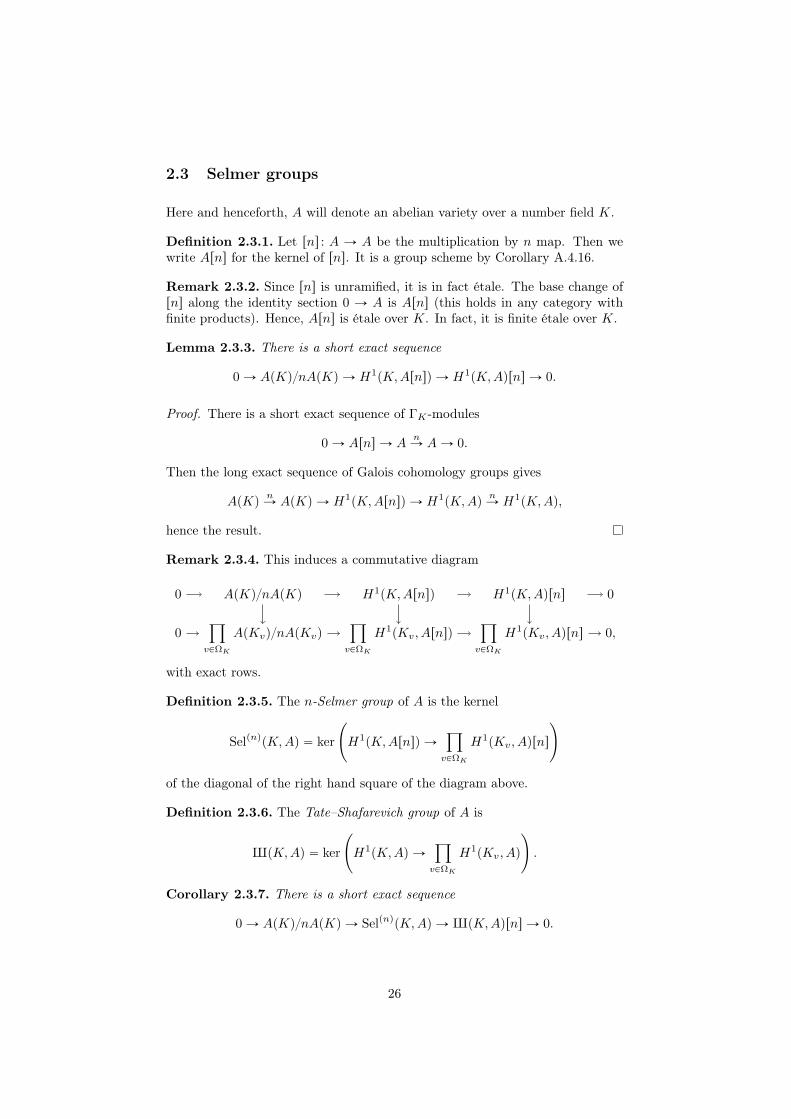
Lemma 2.3.3. There is a short exact sequence

0 Ñ ApKqnApKq Ñ H1pK,Arnsq Ñ H1pK,Aqrns Ñ 0.

Proof. There is a short exact sequence of ΓK-modules

0 Ñ Arns Ñ AnÑ AÑ 0.

Then the long exact sequence of Galois cohomology groups gives

ApKqnÑ ApKq Ñ H1pK,Arnsq Ñ H1pK,Aq

nÑ H1pK,Aq,

hence the result.

Remark 2.3.4. This induces a commutative diagram

0 ApKqnApKq H1pK,Arnsq H1pK,Aqrns 0

0ź

vPΩK

ApKvqnApKvqź

vPΩK

H1pKv, Arnsqź

vPΩK

H1pKv, Aqrns 0,

with exact rows.

Definition 2.3.5. The n-Selmer group of A is the kernel

SelpnqpK,Aq “ ker

˜

H1pK,Arnsq Ñź

vPΩK

H1pKv, Aqrns

¸

of the diagonal of the right hand square of the diagram above.

Definition 2.3.6. The Tate–Shafarevich group of A is

XpK,Aq “ ker

˜

H1pK,Aq Ñź

vPΩK

H1pKv, Aq

¸

.

Corollary 2.3.7. There is a short exact sequence

0 Ñ ApKqnApKq Ñ SelpnqpK,Aq ÑXpK,Aqrns Ñ 0.

26

Proof. Restrict the short exact sequence of the lemma to the elements that mapto zero in the bottom right term

ź

vPΩK

H1pKv, Aqrns

of the commutative diagram above.

Remark 2.3.8. One can show that SelpnqpK,Aq is finite. The proof is essen-tially the same as that of the weak Mordell–Weil theorem. For an elliptic curve,it is given in Theorem X.4.2(b) of Silverman [20].

In particular, XpK,Aqrns is finite. There is the following conjecture.

Conjecture 2.3.9. (Shafarevich–Tate) The group XpK,Aq is finite.

Remark 2.3.10. Since XpK,Aq lives inside H1pK,Aq, it is torsion. Therefore,the conjecture breaks up into two statements:

• XpK,Aqrps “ 0 for almost all primes p,• XpK,Aqtpu is finite for all primes p.

Only in particular cases are we able to compute XpK,Aqtpu, so we are stillquite far away from proving the conjecture.

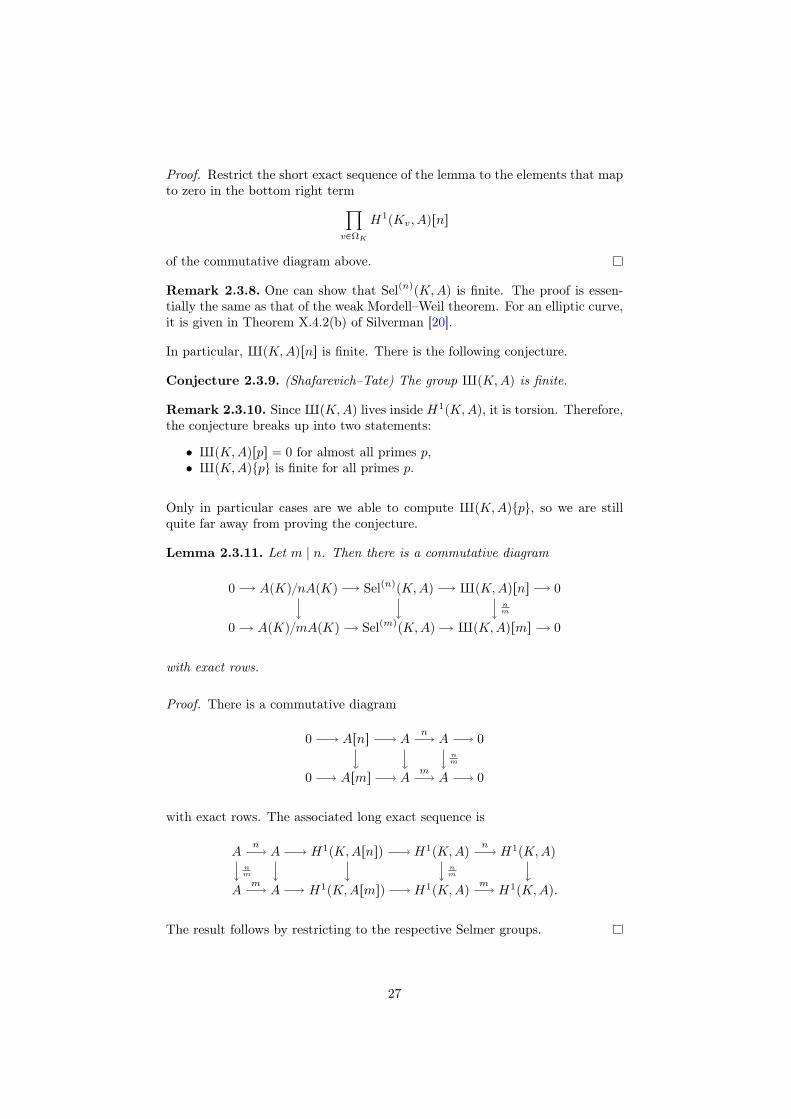
Lemma 2.3.11. Let m | n. Then there is a commutative diagram

0 ApKqnApKq SelpnqpK,Aq XpK,Aqrns 0

0 ApKqmApKq SelpmqpK,Aq XpK,Aqrms 0

nm

with exact rows.

Proof. There is a commutative diagram

0 Arns A A 0

0 Arms A A 0

n

nm

m

with exact rows. The associated long exact sequence is

A A H1pK,Arnsq H1pK,Aq H1pK,Aq

A A H1pK,Armsq H1pK,Aq H1pK,Aq.

n

nm

n

nm

m m

The result follows by restricting to the respective Selmer groups.

27

Definition 2.3.12. Write ApKq for the limit

ApKq “ limÐÝn

ApKqnApKq.

Also, putxSelpK,Aq “ lim

ÐÝn

SelpnqpK,Aq,

where the limit is taken over the maps above. Finally, if B is any abelian group,put

TB “ limÐÝn

Brns

for the (absolute) Tate module of B, where the limit is taken with respect tothe maps

BrnsnmÝÑ Brms

for m | n.

Proposition 2.3.13. Let I be a directed set, and let

0 Ñ pAiq Ñ pBiq Ñ pCiq Ñ 0

be a short exact sequence of projective systems. Then there is an exact sequence

0 Ñ limÐÝi

Ai Ñ limÐÝi

Bi Ñ limÐÝi

Ci.

If moreover I is countable and the maps Ai Ñ Aj for j ď i are surjective, thenthe sequence is exact on the right as well, i.e. lim

ÐÝBi Ñ lim

ÐÝCi is surjective.

Proof. Note that the limit of a projective system pMiq is given by

limÐÝi

Mi “ ker

˜

ź

jďi

MjψÝÑ

ź

i

Mi

¸

,

where ψ is the map given by

pmjqj,i ÞÝÑ pmj ´ miq,

where mi denotes the image of mi in Mj under the natural map Mi Ñ Mj .Then the limits of pAiq, pBiq and pCiq are the kernels of the vertical maps inthe diagram

0ź

jďi

Ajź

jďi

Bjź

jďi

Cj 0

0ź

i

Aiź

i

Biź

i

Ci 0,

ψA ψB ψC

and the first statement follows from taking vertical kernels.

Now if I is countable, say I “ ti0, . . .u, we inductively construct a subset J Ď Iof the form tj0, . . .u such that ik ď jk and the map k ÞÑ jk gives an isomorphismof ordered sets Zě0

„ÝÑ J .

28

Namely, pick j0 “ i0, and inductively let jk be such that jk´1 ď jk and ik ď jk.Such jk exists since I is directed, and it is clear that J satisfies the promisedproperties. We shall identify Zě0 with J via k ÞÑ jk.

Now J is cofinal since ik ď jk for all k P Zě0, so

limÐÝiPI

Mi “ limÐÝkPZě0

Mk

for any projective system pMiq. Moreover, the order on J is linear, so

limÐÝk

Mk “ ker

˜

ź

k

Mk∆ÝÑ

ź

k

Mk

¸

,

where ∆ is the map given by

pmkqk ÞÝÑ pmk ´ mk`1qk,

where mk`1 denotes the image of mk`1 in Mk under the map Mk`1 ÑMk. Wenow get a commutative diagram with exact rows

0ź

k

Akź

k

Bkź

k

Ck 0

0ź

k

Akź

k

Bkź

k

Ck 0.

∆A ∆B ∆C

If pakqk is given, set m0 “ a0 and inductively pick some mk`1 P Ak`1 suchthat mk`1 “ mk ´ ak. We can do this since Ak`1 Ñ Ak is surjective. Then bydefinition

∆A ppmkqkq “ pmk ´ mk`1qk “ pakqk.

Since pakqk was arbitrary, this shows that ∆A is surjective. The result nowfollows from the snake lemma.

Corollary 2.3.14. There is a short exact sequence

0 Ñ ApKq Ñ xSelpK,Aq Ñ TXpK,Aq Ñ 0.

If moreover XpK,Aqdiv “ 0, then ApKq – xSelpK,Aq.

Proof. The first statement follows from the proposition, as the maps

ApKqnApKq ÝÑ ApKqmApKq

for m | n are surjective.

The second statement follows as TB “ T pBdivq for any abelian group B. Indeed,if

pbnqnPZą0P TB Ď

ź

nPZą0

Brns

then that means exactly thatmbmn “ bn

for all m,n P Zą0. Hence, each bn is divisible, so pbnqn P T pBdivq.

29

Lemma 2.3.15. Let B be a torsion abelian group such that Brns is finite forall n P Zą0. Then Bdiv is a divisible group, so in particular it is the maximaldivisible subgroup of B.

Proof. Let b P Bdiv be given, then there exist bn P B such that nbn “ b. Whatwe have to prove is that we can take bn to be in Bdiv.

Let d be the order of b. Then any bn with nbn “ b has order nd. Hence, thesubsets

Cn “

cn P Brdnsˇ

ˇ ncn “ b(

of Brdns are all nonempty. Moreover, there are natural maps

Cmn ÝÑ Cn

cmn ÞÝÑ mcmn

for all m,n. Since Brdns is finite, so is Cn. Since a projective limit of finitenonempty sets is nonempty, there exists an element pcnq P lim

ÐÝCn Ď TB such

that ncn “ b for all n. Saying that pcnq P limÐÝ

Cn means that mcmn “ cn for allm,n, hence each cn is divisible. Hence, b is divisible in Bdiv as well.

Remark 2.3.16. The lemma is no longer valid if we drop the assumption thatBrns be finite. Indeed, let B be the quotient of the group

à

n

xnpZ2nZq

by the subgroup generated by nxn ´ x1. Then B is a torsion group, and x1 isdivisible by construction (and it has order 2). However, no other xn is divisible,and in fact one can show that Bdiv “ t0, x1u. This is clearly not a divisiblegroup.

What happens here is that we can find xn with nxn “ x1, but we can not dothis in a compatible way, i.e. we do not have mxmn “ xn.

Corollary 2.3.17. We have ApKq “ xSelpK,Aq if and only if XpK,Aqdiv “ 0.

Proof. One implication was already noted in Corollary 2.3.14. Conversely, ifApKq “ xSelpK,Aq, then TXpK,Aq “ 0. The proof of the lemma above showsthat if Bdiv ‰ 0, then TB ‰ 0. Since XpK,Aqrns is finite for each n, we canapply this to B “XpK,Aq to obtain the result.

Remark 2.3.18. The article of Stoll [22] uses the notation Bdiv to mean themaximal divisible subgroup of an abelian group B, as opposed to the set ofdivisible elements. By the lemma above, in the case of XpK,Aq there is nodifference.

Finally, we will compare ApAKq with ApAKq‚ (see section 1.3 for this notation).

Proposition 2.3.19. There is a short exact sequence

0 Ñ ApAKqdiv Ñ ApAKq Ñ ApAKq‚ Ñ 0.

30

Proof. There is a short exact sequence

0 Ñź

vPΩ8K

ApKvq0 Ñ ApAKq Ñ ApAKq‚ Ñ 0

induced by the short exact sequences

0 Ñ ApKvq0 Ñ ApKvq Ñ π0pApKvqq Ñ 0

for v P Ω8K . Here, ApKvq0 denotes the connected component of the origin,

which is a (normal) subgroup with quotient π0pApKvqq. Note that since A isconnected, the complex places give a trivial π0, so they do not contribute toApAKq‚ (compare Remark 1.3.9).

It remains to prove that ApKvq0 “ ApKvqdiv for all infinite places v and

ApKvqdiv “ 0 for all finite places v. But ApAKq‚ is compact and totally discon-nected, hence profinite. Hence, it contains no divisible elements, so

ApKvqdiv Ď ApKvq0

for all infinite places, and ApKvqdiv “ 0 for all finite places.

Finally, a standard result on real or complex Lie groups shows that for a compactLie group, the exponential

exp: LiepApKvqq Ñ ApKvq

is a surjection onto ApKvq0. Hence, every element of ApKvq is divisible, so

ApKvqdiv “ ApKvq0,

which finishes the proof.

Corollary 2.3.20. Let n P Zą0. Then

ApAKqnApAKq “ ApAKq‚nApAKq‚.

Proof. Take vertical cokernels in the diagram

0 ApAKqdiv ApAKq ApAKq‚ 0

0 ApAKqdiv ApAKq ApAKq‚ 0.

n n n

The result then follows since the left vertical map is surjective.

Corollary 2.3.21. There is a natural identification

ApAKq – ApAKq‚.

Proof. This follows since ApAKq‚ is its own profinite completion.

31

Lemma 2.3.22. There is a chain of maps

ApKq ãÑ ApKq ãÑ xSelpK,Aq Ñ ApAKq‚,

inducing isomorphisms

ApKqtors„Ñ ApKqtors

„Ñ xSelpK,Aqtors.

Proof. By the definition of the Selmer group, there are maps

SelpnqpK,Aq Ñź

v

ApKvqnApKvq.

These induce a map xSelpK,Aq Ñ ApAKq by taking the limit, and the right handside is ApAKq‚ by the corollary above.

By the Mordell–Weil theorem, there is an isomorphism

ApKq – ∆ˆ Zr

for some finite group ∆ and some r P Zě0. In particular, ApKqdiv “ 0, so themap ApKq Ñ ApKq is injective. Injectivity of ApKq Ñ xSelpK,Aq is Corollary2.3.14.

Finally, the explicit description of ApKq also gives

ApKq – ∆ˆ Zr,

so ApKqtors “ApKqtors. The identification

ApKqtors “xSelpK,Aqtors

follows from Corollary 2.3.14, taking into account that pTBqtors “ 0 for anyabelian group B.

The main result of the next section (and indeed one of the main results of thiswork) is that the map

xSelpK,Aq Ñ ApAKq‚is also injective.

2.4 Adelic points of abelian varieties

This section is essentially section 3 of Stoll’s paper [22]. Its main ingredient isa theorem of Serre (which we will not prove); see Theorem 2.4.2.

Lemma 2.4.1. Let AK be an abelian variety. Then there is an isomorphism

AutpAtorsq – GL2gpZq

of groups.

32

Proof. Over the complex numbers, there is an isomorphism

ApCq – CgΛ,

for some lattice Λ Ď Cg. Since multiplication by n is defined over K, all n-torsion of A is defined over K. That is,

ApKqtors – ApCqtors “ pQZq2g.

Since QZ is the colimit of 1nZZ, we get

HomppQZq2g, pQZq2gq “ limÐÝn

Hompp 1nZZq

2g, pQZq2gq

“ limÐÝn

Hompp 1nZZq

2g, p 1nZZq

2gq

“ limÐÝn

M2gpZnZq “M2gpZq.

Taking invertible elements gives the result.

Theorem 2.4.2. Let AK be an abelian variety. Then the image of ΓK Ñ

GL2gpZq contains a subgroup pZˆqd of d-th power scalars, for some d P Zą0.

Proof. See [17].

Lemma 2.4.3. Let d P Zą0 be even, and let S “ pZˆqd Ď Zˆ. Let Zˆ –

AutpQZq act on QZ in the canonical way. Then there exists D P Zą0 killing

HipS,QZq,

for i P t0, 1u.

Proof. For p prime, put νp “ mintvppad ´ 1q | a P Zˆp u. Put

D “ź

p

pνp ,

and note that this indeed a finite product, for instance since, for p ‰ 2,

νp ď vpp2d ´ 1q,

which is zero for almost all p. There is a decomposition

QZ –à

p

pQZqtpu “à

p

QpZp.

Since any isomorphism has to map the p-primary torsion into the p-primarytorsion, the restriction of the action of Zˆ to QpZp is just given by the action ofthe subgroup Zˆp Ď Zˆ. One easily sees that in fact this is just the multiplicationaction of Zˆp on QpZp.

We have a decomposition

pQZqS “à

p

pQpZpqpZˆp qd

.

33

By definition, each term of the right hand side is given by

pQpZpqpZˆp qd

“ tx P QpZp | pad ´ 1qx “ 0 for all a P Zˆp u.

Hence, if ap is an element such that vppadp´1q is minimal, any x P pQpZpqpZˆp qd

is killed by adp ´ 1, hence also by pνp . Hence, pQZqS is killed by D.

Now the logarithm induces isomorphisms

Zˆ2„ÝÑ t˘1u ˆ Z2,

Zˆp„ÝÑ Zpp´ 1qZˆ Zp pp oddq.

Since d is even, this gives isomorphisms (including for p “ 2)

pZˆp qd„ÝÑ dpZpp´ 1qZˆ Zpq.

In particular, pZˆp qd has a topological generator α, corresponding to the element

d ¨ p1, 1q P dpZpp´ 1qZˆ Zpq.

Since α generates pZˆp qd topologically, any continuous 1-cocycle

a : pZˆp qd Ñ QpZp

is uniquely determined by its value at α. Moreover, it comes from the cobound-ary σ ÞÑ σb´ b if and only if aα “ pα´ 1qb. This gives an injection

H1ppZˆp qd,Qp,Zpq ãÑQpZp

pα´ 1qQpZp.

Since α´ 1 ‰ 0 and since QpZp is divisible (by elements of Zp, even), the righthand side is 0. Hence,

H1ppZˆp qd,QpZpq “ 0.

Also, the action ofś

q‰p Zˆq on QpZp is trivial, so

H1

˜

ź

q‰p

pZˆq qd,QpZp

¸pZˆp qd

“ Homcont

˜

ź

q‰p

pZˆq qd,QpZp

¸pZˆp qd

“ Homcont

˜

ź

q‰p

pZˆq qd, pQpZpqpZˆp qd

¸

.

The latter is killed by D since pQpZpqpZˆp qd

is. The inf-res sequence gives

0 Ñ H1ppZˆp qd,QpZpq Ñ H1pS,QpZpq Ñ H1

˜

ź

q‰p

pZˆq qd,QpZp

¸pZˆp qd

.

The left term is zero, and the right term is killed by D. Hence, the middle termis killed by D as well. Taking the sum over all primes gives the result.

34

Definition 2.4.4. Let AK be an abelian variety. Put

Kn “ KpArnsq

for the field obtained by adjoining (all coordinates of) the n-torsion to K. Alsoput

K8 “8ď

n“1

Kn.

Remark 2.4.5. Note that KnK is a finite extension. Moreover, if nP “ 0,then nσpP q “ σpnP q “ 0 as well, for σ P ΓK . Hence, KnK is Galois. It followsthat also K8K is Galois.

Proposition 2.4.6. Let AK be an abelian variety. Then there exists m P Zą0

killing all H1pKnK,Arnsq.

Proof. Note that K8 is defined to be the fixed field of the kernel of ΓK Ñ

GL2gpZq. Hence, the image of this morphism is isomorphic to G “ GalpK8Kq.By Theorem 2.4.2, it contains S “ pZˆqd for some d P Zą0. By making S smallerif necessary, we can assume that d is even. Then by the lemma above, thereexists D P Zą0 killing

HipS,Atorsq “ pHipS,QZqq2g

for i P t0, 1u.

Since S is central in GL2gpZq, it is normal in G. Then the inf-res sequence gives

0 Ñ H1pGS,AStorsq Ñ H1pG,Atorsq Ñ H1pS,Atorsq.

The first term is killed by D since AStors is, and the third term is also killed byD. Hence, the middle term is killed by D2.

Now the short exact sequence

0 Ñ Arns Ñ Ators Ñ Ators Ñ 0

of G-modules (note that all torsion is defined over K8) gives a long exactsequence

. . .Ñ ApKqtors Ñ H1pK8K,Arnsq Ñ H1pK8K,Atorsq Ñ . . . .

The third term is killed by D2, and the first term is finite. Hence, the middleterm is killed by

m “ #ApKqtors ¨D2.

Finally, the inflation map gives an injection

H1pKnK,Arnsq ãÑ H1pK8K,Arnsq,

which gives the result.

35

Corollary 2.4.7. The kernel of

SelpnqpK,Aq Ñ SelpnqpKn, Aq

is killed by m.

Proof. There is an inf-res sequence

0 Ñ H1pKnK,Arnsq Ñ H1pK,Arnsq Ñ H1pKn, Arnsq. (2.4)

By definition, the Selmer groups live inside the second and third term, and themap SelpnqpK,Aq Ñ SelpnqpKn, Aq is the one induced by (2.4). Hence, the kernelis killed by m, since H1pKnK,Arnsq is.

Lemma 2.4.8. Let Q P SelpnqpK,Aq, and let α be the image of Q under themap

SelpnqpK,Aq Ñ SelpnqpKn, Aq Ď H1pKn, Arnsq “ HomcontpΓKn , Arnsq.

Let L be the fixed field of the kernel of α. Let v be a place of K that splitscompletely in Kn. Then v splits completely in L if and only if the image of Qin ApKvqnApKvq is zero.

Proof. Let w be a place of Kn above v. Then v splits completely in L iff w does,and the latter is equivalent to

αˇ

ˇ

ΓKn,w“ 0.

We have a commutative diagram

SelpnqpK,Aq SelpnqpKn, Aq HompΓKn , Arnsq

ApKvqnApKvq ApKn,wqnApKn,wq HompΓKn,w , Arnsq.

The result follows since both horizontal arrows of the right hand square areinjections and the bottom arrow of the left hand square is an isomorphism.

Lemma 2.4.9. Let Q P SelpnqpK,Aq, and let d be the order of mQ. Then thedensity of places v of K such that v splits completely in Kn and the image of Qin ApKvqnApKvq is trivial is at most 1

drKn:Ks .

Proof. Let α : ΓKn Ñ Arns and L be as in the lemma above. Let e be the orderof α.

By Corollary 2.4.7, the kernel of

SelpnqpK,Aq Ñ SelpnqpKn, Aq

is killed by m. Since eα “ 0, it follows that eQ is in this kernel, so meQ “ 0.Since d is the order of mQ, this forces d | e.

36

On the other hand, one can easily see that the order of α is the exponent of itsimage. That is,

e “ exppGalpLKnqq.

In particular, it divides rL : Kns. Hence, d | e | rL : Kns, so

rL : Ks “ rL : KnsrKn : Ks ě d ¨ rKn : Ks.

The result now follows from the lemma above and Chebotarev’s Density Theo-rem.

Lemma 2.4.10. Let I be a directed set, and let pBiq be some projective system.Put B “ lim

ÐÝBi. Let b1, . . . , br P B have infinite order, and let d P Zą0 be given.

Then there exists i P I such that the images of b1, . . . , br all have order at leastd in Bi.

Proof. The elements pd´ 1q!bk P B are nonzero, so there exist ik P I such thatpd´ 1q!pbkqik P Bik is nonzero.

Since I is directed, there exists i P I with i ě ik for all k P t1, . . . , ru. Then

pd´ 1q!pbkqi ‰ 0 P Bi.

Hence, each pbkqi has at least order d.

Theorem 2.4.11. Let Z Ď A be a finite subscheme of A such that ZpKq “ZpKq. Let P P xSelpK,Aq be such that the image Pv of P in ApKvq is insideZpKvq “ ZpKq for a set of finite places v of density 1. Then P P ZpKq.

Proof. Let d ą #ZpKq. Write

P ´ ZpKq “ tQ1, . . . , Qru Ď xSelpK,Aq.

Note that the assumption on P is that there is a set of finite places v of density1 such that one of the Qi maps to 0 in ApKvq.

Now suppose that all the Qi have infinite order. Then so do the mQi, so by thelemma above, there exists n P Zą0 such that the image of mQi in SelpnqpK,Aqhas order di ě d for all i P t1, . . . , ru. By Lemma 2.4.9, the set of places ofK that split completely in Kn such that the image of at least one of the Qi inApKvqnApKvq is trivial is at most

rÿ

i“1

1

dirKn : Ksď

r

drKn : Ksă

1

rKn : Ks.

Hence, there is a set of places of positive density that split completely, but forwhich the images of all the Qi in ApKvqnApKvq are nonzero. This contradictsthe assumption on P , so at least one of the Qi must have finite order. Hence

P P ZpKq ` xSelpK,Aqtors “ ZpKq `ApKqtors Ď ApKq.

37

Now pick a finite place such that Pv P ZpKvq “ ZpKq. Since the map

ApKq Ñ ApKvq

is injective and P lands inside ZpKvq “ ZpKq, in fact P itself is in ZpKq.

Theorem 2.4.12. Let AK be an abelian variety, and let S be a set of placesof K of density 1. Then the map

xSelpK,Aq Ñ ApASKq‚

is injective.

Proof. We can without loss of generality remove the infinite places from S. Thenapply the proposition above to the finite subscheme Z “ t0u.

Corollary 2.4.13. The map

ApKq Ñ ApAKq‚

induces an identification between ApKq and the topological closure ApKq ofApKq in ApAKq‚.

Proof. The map is injective by the above, and it is continuous since it wasdefined via the quotients

ApKqnApKq Ñ ApAKqnApAKq.

It is a closed map since ApKq is compact and ApAKq‚ is Hausdorff, so thetopology on ApKq is just the subspace topology of the closed subset ApKq Ď

ApAKq‚. The result follows since ApKq is dense in ApKq.

Corollary 2.4.14. Let LK be finite. Then the map

xSelpK,Aq Ñ xSelpL,Aq

is injective.

Proof. Let S “ ΩfK be the set of finite places. Then we have a commutativediagram

xSelpK,Aq ApAfKq‚

xSelpL,Aq ApAfLq‚.

The two horizontal maps are injective by the theorem, and the right verticalmap is injective since ApAfKq‚ is just ApAfKq. Hence, the left vertical map isinjective as well.

38

Remark 2.4.15. This last corollary can also be proven directly from the def-initions. Together with the theorem, it allows us to think of all the arrows inthe diagram

ZpKq ApKq ApKq xSelpK,Aq ApASKq‚

ZpLq ApLq zApLq xSelpL,Aq ApATLq‚

as inclusions, whenever S Ď ΩfK is a set of finite places of density 1 and T isthe set of places of L above S.

For more flexibility, we remove from Theorem 2.4.11 the restriction that allpoints of Z are defined over K.

Theorem 2.4.16. Let Z Ď A be a finite subscheme. Let P P xSelpK,Aq be suchthat the image Pv P ApKvq is inside ZpKvq for a set S of finite places v of Kof density 1. Then P P ZpKq.

Proof. Since Z is a finite scheme, there is a finite Galois extension LK such thatZpLq “ ZpKq. Theorem 2.4.11 then implies that the image of P in xSelpL,Aq isinside ZpLq.

But the image of P in ApATLq‚ is GalpLKq-stable since it comes from ApASKq‚(where T is the set of places of L above S). Hence,

P P ZpLqGalpLKq “ ZpKq.

Remark 2.4.17. The proof uses that ZpLqGalpLKq “ ZpKq. I do not knowwhether the analogous statement for xSelpK,Aq is true as well, i.e. whether theintersection of xSelpL,Aq and ApASKq‚ inside ApATLq‚ is xSelpK,Aq.

2.5 Jacobians

We will not prove the existence of Jacobians, but we will state the definitionsand main properties, as well as some results we will need later on.

Theorem 2.5.1. Let C be a curve of genus g over a field K. Then there existsan abelian variety J of dimension g together with a map

Pic0pC ˆK Lq Ñ JpLq

for all LK finite separable (functorial in L) that is an isomorphism wheneverCpLq ‰ ∅. Moreover, J is unique up to a unique isomorphism, and is calledthe Jacobian of C.

Proof. See e.g. [14], Theorem III.1.6.

39

Theorem 2.5.2. Let C be a curve over K, and let LK be a finite separa-ble extension such that CpLq ‰ ∅. Then any point P gives rise to a closedimmersion

fP : C ˆK L ÝÑ J ˆK L,

which on M -points (for ML finite separable) is given by

CpMq ÝÑ Pic0pC ˆK Mq – JpMq

Q ÞÝÑ rQ´ P s.

Proof. See [14], Proposition III.2.3.

Remark 2.5.3. Note that the map fP only depends on P up to translation.That is,

fP1

“ τrP´P 1s ˝ fP ,

for P, P 1 P CpLq.

Remark 2.5.4. For C “ E an abelian variety of dimension 1, one sees that Eis its own Jacobian. Since the dimension of J is the genus of C, this shows thatE has genus 1, hence is an elliptic curve.

We will now turn to Jacobians over the real numbers. In what follows, C willbe a curve over R such that CpRq ‰ ∅.

Lemma 2.5.5. Let x1, x2 P CpRq be distinct points. Then there exists a func-tion f P RpCq with no real poles, such that fpx1q ‰ fpx2q.

Proof. Since CpCq is a complex manifold, it is also a real manifold of dimension2. Hence, as CpRq Ď CpCq has real dimension 1, there exist infinitely manypoints P P CpCq that are not in CpRq. Fix such a P , and consider the divisorD “ npP ` P q ´ x1, for some n, where P is the complex conjugate of P . Notethat D is defined over R.

If 2n´ 1 ą g ` 1, then Riemann–Roch shows that

h0pC,L pDqq “ degD “ 2n´ 1,

andh0pC,L pD ´ x2qq “ degpD ´ x2q “ 2n´ 2.

Hence, there exists a function f P RpCq such that div f ` D is effective, butdiv f `D´ x2 is not. Hence, div f `D contains no terms x2, so div f containsno terms x2.

Then f is an element of RpCq, and f has only poles at the non-real points Pand P . Moreover, it has a zero at x1, and neither a zero nor a pole at x2.

Corollary 2.5.6. The set of functions f P RpCq with no real poles is dense inMappCpRq,Rq, with respect to the topology of uniform convergence.

Proof. This is the Stone–Weierstrass theorem, applied to the compact spaceCpRq.

40

Proposition 2.5.7. Let C1, . . . , Cr be the connected components of CpRq. Thenthere exists a function f P RpCq with no real zeroes or poles such that f isnegative on C1 and positive on all other Ci.

Proof. We can create a sequence pfnq of functions uniformly converging to thefunction that is ´1 on C1 and 1 on the other Ci. Hence, eventually fn will benegative on all of C1 and positive on all of Ci. Note that f then automaticallyhas no real zeroes.

Proposition 2.5.8. Suppose that P,Q P CpRq are two real points such thatrP ´ Qs is divisible by 2. Then P and Q lie in the same connected componentof CpRq.

Proof. Let C1, . . . , Cr be the connected components of CpRq, in such a way thatP P C1. By the proposition above, there exists f P RpCq such that f has neitherzeroes nor poles on CpRq and f is negative on C1 and positive on all other Ci.Since all zeroes and poles of f are non-real, they come in pairs, and div f is ofthe form

ÿ

i

nipPi ` Piq.

Now if rP ´ Qs is divisible, there exists a divisor M and an element g P CpCqsuch that P ´Q “ 2M ` div g. Hence,

fpP q

fpQq“ fp2Mq ¨ fpdiv gq.

Note that fp2Mq “ fpMq2, which is always nonnegative. Moreover, a standardresult shows that fpdiv gq “ gpdiv fq. Since div f is of the form

ÿ

i

nipPi ` Piq,

this givesgpdiv fq “

ź

i

pfpPiqfpPiqqni “

ź

i

pfpPiqfpPiqqni ,

which is nonnegative as well. Hence,

fpP q

fpQq“ fpMq2gpdiv fq ě 0.

Since P P C1, we have fpP q ă 0. Hence, fpQq is negative as well, so Q P C1.

Corollary 2.5.9. Let C be a curve over R, such that CpRq ‰ ∅. Then the map

π0pCpRqq Ñ π0pJpRqq

induced by the embedding of C into its Jacobian J is injective.

Proof. We saw in the proof of Proposition 2.3.19 that JpRq0 “ JpRqdiv, i.e. theidentity component of the Jacobian is the subgroup of divisible elements. Now ifP,Q P CpRq map to the same component of JpRq, then rP´Qs is in the identitycomponent, hence it is divisible. Hence, P and Q lie in the same component ofCpRq.

41

Corollary 2.5.10. Let K be a number field, and let C be a curve over K withCpKq ‰ ∅. Then the map

CpAKq‚ Ñ JpAKq‚

induced by the embedding of C into its Jacobian J is injective.

Proof. At the finite places and the complex places, there is nothing to prove.At the real places, it follows from the corollary above.

42

3 Torsors

In this chapter, we will look closely at the first cohomology of representablesheaves of abelian groups. We will give an ad hoc definition of H1 for sheavesof (not necessarily commutative) groups, and show that its elements correspondto certain geometrical objects.

3.1 First cohomology groups

Lemma 3.1.1. Let G : B Ñ A be a functor with an exact left adjoint F . ThenG preserves injectives.

Proof. Let I P ob B be injective. Let 0 Ñ AÑ B be an injection in A . Then

0 Ñ FAÑ FB

is exact in B. Hence, the map

BpFB, Iq Ñ BpFA, Iq

is surjective. But this is A pB,GIq Ñ A pA,GIq, by the adjunction.

In order to compute the first cohomology, we want to use Čech cohomology. Inorder to do this, we need some comparison results between Čech cohomologyand sheaf cohomology.

Proposition 3.1.2. Let I be an injective presheaf, and let U “ tUi Ñ UuiPIbe a covering of some U P ob C . Then HipU ,I q “ 0 for all i ą 0.

Proof. This is Lemma III.2.4 of [15].

Theorem 3.1.3. The functors HipU ,´q : PShpC q Ñ PShpC q are the rightderived functors of H0pU ,´q.

Proof. Note that for a short exact sequence of presheaves

0 Ñ F Ñ G Ñ H Ñ 0,

we get a commutative diagram

0 0 0

0 F pUqś

iPI F pUiqś

pi,jqPI2 F pUi ˆU Ujq . . .

0 G pUqś

iPI G pUiqś

pi,jqPI2 G pUi ˆU Ujq . . .

0 H pUqś

iPI H pUiqś

pi,jqPI2 H pUi ˆU Ujq . . . ,

0 0 0

44

with exact columns. That is, we have an exact sequence

0 Ñ C‚pU ,F q Ñ C‚pU ,G q Ñ C‚pU ,H q Ñ 0

of chain complexes.

This gives a long exact cohomology sequence

0 Ñ H0pU ,F q Ñ H0pU ,G q Ñ H0pU ,H q Ñ H1pU ,F q Ñ . . . .

The result now follows from the definition of right derived functor by a routinecomputation, since any injective sheaf is acyclic by the proposition above.

Proposition 3.1.4. Let F be a sheaf. Then there is an isomorphism

H 1pF q –H 1pF q.

Proof. Note that the inclusion ShpC q Ñ PShpC q preserves injectives by Lemma3.1.1, since it has an exact left adjoint by Theorem B.3.6 and Proposition B.3.17.

Now let F Ñ I be a monomorphism into an injective sheaf I . Let G be thepresheaf cokernel, then G` is the sheaf cokernel (Corollary B.3.10). Moreover,G is separated by Lemma B.3.14. The long exact sequence of H i gives an exactsequence

0 Ñ F Ñ I Ñ G` Ñ H 1pF q Ñ 0 (3.1)

in PShpC q, since I is injective. On the other hand, since G is separated, wehave H 0pG q “ G`, so the short exact sequence of presheaves

0 Ñ F Ñ I Ñ G Ñ 0

gives the long exact H i-sequence

0 Ñ F Ñ I Ñ G` Ñ H 1pF q Ñ 0,

since I is also injective as presheaf. Comparing with (3.1) gives the result.

3.2 Nonabelian cohomology

We give an ad hoc definition of H1pU,G q when G is a sheaf of (not necessarilyabelian) groups.

Definition 3.2.1. Let G be a sheaf of groups on a site C , and let U “ tUi ÑUuiPI be a covering of some U P ob C . Then a 1-cocycle for U with values inG is a family

pgijqpi,jq Pź

pi,jqPI2

G pUijq

satisfying´

gijˇ

ˇ

Uijk

¯

¨

´

gjkˇ

ˇ

Uijk

¯

“ gikˇ

ˇ

Uijk,

for all pi, j, kq P I3, where the product is the group law of G pUijkq. We willusually write g for the cocycle pgijqpi,jq.

45

Definition 3.2.2. Let g, h be two 1-cocycles. Then g is cohomologous to h ifthere exists a family b “ pbiqi P

ś

iPI G pUiq such that

hij “´

biˇ

ˇ

Uij

¯

¨ gij ¨´

bjˇ

ˇ

Uij

¯´1

,

for all pi, jq P I2. This is clearly an equivalence relation, and the set of coho-mology classes is denoted

H1pU ,G q.

It is called the first cohomology of G with respect to U .

Remark 3.2.3. If G is a sheaf of abelian groups, then H1pU ,G q was alreadydefined, namely as the cohomology of the complex

C0pU ,G q Ñ C1pU ,G q Ñ C2pU ,G q.

The map d1 : C1pU ,G q Ñ C2pU ,G q is defined by

pgijqpi,jq ÞÑ´´

gjkˇ

ˇ

Uijk

¯

´

´

gikˇ

ˇ

Uijk

¯

`

´

gijˇ

ˇ

Uijk

¯¯

pi,j,kq,

hence a 1-cocycle is exactly an element of ker d1. The map d0 is given by

pbiqi ÞÑ´

bjˇ

ˇ

Uij

¯

´

´

biˇ

ˇ

Uij

¯

,

hence two 1-cocycles g, h are cohomologous if and only if their difference is inim d0. Hence, the definition of H1pU ,G q given here is the same as the one givenin section B.2.

Remark 3.2.4. Just like in the abelian case, if V is a refinement of U , thereis a natural morphism

H1pU ,G q Ñ H1pV ,G q.

We defineH1pU,G q “ colim

ÝÑU PJU

H1pU ,G q.

We have already seen in Remark B.2.14 that JU is a directed set, so the colimitis just a direct limit.

Definition 3.2.5. A sequence

1 Ñ F Ñ G Ñ H Ñ 1

of sheaves of groups is exact if for every U P ob C , the sequence

1 Ñ F pUq Ñ G pUq ÑH pUq

is exact, and for every h P H pUq, there exists a covering U “ tUi Ñ Uu of Usuch that the restrictions h|Ui come from elements gi P G pUiq.

Remark 3.2.6. For the case where F , G and H are all sheaves of abeliangroups, this notion corresponds to the notion of exactness in the abelian categoryShpC q, by Corollary B.3.7 and Corollary B.3.13.

46

In general, analogously to Theorem B.3.6 and Corollary B.3.7, one can see thatlimits in the category of sheaves of groups are just pointwise. This justifiesthe first part of the definition of exactness. In general one would hope thatCorollary B.3.13 generalises to the statement that regular epimorphisms in thecategory of sheaves of groups are exactly the G Ñ H satisfying the second partof the definition of exactness. We do not prove this, and we will use the ad hocnotion of surjectivity instead.

Proposition 3.2.7. Let 1 Ñ F Ñ G Ñ H Ñ 1 be a short exact sequence, andlet U P ob C . Then there is a long exact sequence of pointed sets

1 Ñ F pUq Ñ G pUq ÑH pUq Ñ H1pU,F q Ñ H1pU,G q Ñ H1pU,H q.

If moreover F is abelian and F Ñ G lands inside the centre (pointwise), thenthis sequence can be extended to

. . .Ñ H1pU,F q Ñ H1pU,G q Ñ H1pU,H q Ñ H2pU,F q.

Proof. See [7], sections III.3 and IV.3.

3.3 Torsors

Definition 3.3.1. Let X be a scheme, and let G be a group scheme over X.Then a sheaf torsor for G on Xet (or Xfppf) is a sheaf of sets S together with aright G-action such that there exists a covering tUi Ñ Xu such that each S |Uet

(resp. S |Ufppf) is isomorphic to GˆX U with the canonical G-action.

We will later turn to the case where S can be represented by some X-schemeS. However, we will firstly characterise sheaf torsors.

Definition 3.3.2. Let S be a sheaf torsor for G. Let U “ tUi Ñ Xu be acovering that trivialises S . Then in particular S pUiq is nonempty for all i, sowe can pick si P S pUiq. Since the action of GˆX U on S pUiq is isomorphic toGˆX U , there exists a unique gij P GpUijq such that

´

siˇ

ˇ

Uij

¯

gij “ sjˇ

ˇ

Uij.

Then´

siˇ

ˇ

Uijk

¯

gijgjk “ sk “´

siˇ

ˇ

Uijk

¯

gik.

Since the action of G on S pUijkq is simply transitive, this forces

gijgjk “ gik,

so g “ pgijq is a 1-cocycle. (We have omitted the restrictions to ease notation.)

Lemma 3.3.3. The cohomology class of g does not depend on the choice of Uor of the si. Moreover, it depends on S only up to isomorphism (of sheaveswith G-action).

47

Proof. If we choose other s1i, then there exist unique bi P GpUiq with s1ibi “ si.Hence, (omitting restrictions to ease notation)

s1ig1ijbj “ s1jbj “ sj “ sigij “ s1ibigij ,

so g1ij “ bigijb´1j , and g and g1 are cohomologous.

Independence of the choice of U follows from independence of the choice ofthe si, taking a common refinement and restricting the chosen si. The laststatement is clear.

Definition 3.3.4. The association of the cocycle g is denoted S ÞÑ gpS q.

Definition 3.3.5. Conversely, let g P H1pX,Gq be a 1-cocycle; say that g PH1pU , Gq for a covering U “ tUi Ñ Xu. Let Fn be the presheaf defined by

FnpV q “ź

pi1,...,inqPIn

GpUi0¨¨¨in ˆX V q,

for n P t0, 1u, and note that it is in fact a sheaf. Let d : F0 Ñ F1 be themorphism given on an arbitrary V by

ź

iPI

GpUi ˆX V q ÝÑź

pi,jqPI2

GpUij ˆX V q

phiqi ÞÝÑ ph´1i hjqi,j .

Now, g is by definition a global section of F1, so it defines elements

gˇ

ˇ

V“

´

gijˇ

ˇ

UijˆXV

¯

i,jPI2P F1pV q.

Then define S as the presheaf inverse image of g. That is, for any V , we have

S pV q “

s P F0pV qˇ

ˇ dpsq “ gˇ

ˇ

V

(

.

Remark 3.3.6. Note that S is in fact a subsheaf of F0: if s P F0pV q is given,and tVi Ñ V u is some covering such that s|Vi P S pViq for all i, then

dpsqˇ

ˇ

Vi“ d

´

sˇ

ˇ

Vi

¯

“ gˇ

ˇ

Vi

for all i, hence by the sheaf condition of F1, we must have dpsq “ g|V , sos P S pV q.

Definition 3.3.7. We equip S with a right G-action in the following way: forany V , we define

S pV q ˆGpV q ÝÑ S pV q

ppsiqiPI , hq ÞÝÑ

ˆ

´

hˇ

ˇ

UiˆXV

¯´1

si

˙

iPI

,

where we think of an element s P S pV q as the element psiqiPI P F0pV q. Notethat if psiq P S pV q, then (once again omitting restrictions)

d``

h´1si˘

i

˘

“`

ph´1siq´1h´1sj

˘

i,j“`

s´1i sj

˘

i,j“ d ppsiqiq .

48

Hence, ph´1siqi is in S pV q as well. Clearly, this gives a right GpV q-action toeach S pV q, and the maps S pV q Ñ S pV 1q are G-invariant, so it indeed givesa G-action on S .

Lemma 3.3.8. The sheaf S with the given right G-action is a torsor. Up toisomorphism, it depends neither on the choice of representative for the cocyclewe started with, nor on the covering U trivialising g.

Proof. For each n P I, we have

gijˇ

ˇ

Uijn“

´

ginˇ

ˇ

Uijn

¯´

gjnˇ

ˇ

Uijn

¯´1

.

Hence, setting spnq “ pspnqi qi “ pg´1in qi P F0pUnq, the above identity reads:

gˇ

ˇ

Un“ d

´

spnq¯

.

That is, S |Un has a global section spnq. But then the morphism of sheavesG|Un Ñ S |Un given on V Ñ Un by

GpV q ÝÑ S pV q

h ÞÝÑ h´1spnqˇ

ˇ

V

gives an isomorphism of sheaves of sets with right G-actions, showing that Untrivialises S . Since tUn Ñ Xu is a covering, this shows that S is a torsor.

Now if g1 is a cohomologous cocycle, then there exists pbiqi P F0pXq such that

g1ij “ bigijb´1j .

Define the maps

f0 : F0pV q ÝÑ F0pV q

phiqi ÞÝÑ phib´1i qi

and

f1 : F1pV q ÝÑ F1pV q

paijqi,j ÞÝÑ pbiaijb´1j qi,j .

This gives a commutative diagram of morphisms of sheaves

F0 F1

F0 F1.

d

f0 „ f1 „

d

Since f1pgq “ g1, this diagram induces an isomorphism S – S 1 of the inverseimages of g and g1 in F0. Since f0 is defined by multiplication on the right, itcommutes with the action of G on S and S 1, which is given on the left. Hence,S – S 1 as G-sheaves, hence as torsors.

49

Hence, S does not depend on the cocycle representing our class. If we chosea different covering U 1, then restricting our cocycles to a common refinementshows that S also does not depend on U .

Definition 3.3.9. The association of the sheaf torsor S is denoted g ÞÑ Sg.

Theorem 3.3.10. The maps S Ñ gpS q and g ÞÑ Sg give a bijection betweenthe set of isomorphism classes of sheaf torsors on Xet (or Xfppf) and H1pXet, Gq(resp. H1pXfppf , Gq).

Proof. If g is a 1-cocycle, say g P H1pU , Gq, then the lemma above shows thatU trivialises g, and there are sections spnq P SgpUnq, defined by

spnqi “ g´1

in .

The cocycle condition on g asserts that (omitting restrictions)

g´1nm g´1

in “ g´1im ,

which by the definition of the G-action on S (Definition 3.3.7) gives

spnqgnm “´

pgnmq´1spnqi

¯

i“

´

spmqi

¯

i“ spmq.

Hence, g is the cocycle gpSgq associated to Sg, by Definition 3.3.2.

Conversely, let S be a sheaf torsor. We fix U “ tUi Ñ XuiPI trivialising S ,and we fix sections si P S pUiq. Then gij is defined by

sigij “ sj .

Moreover, the isomorphism of sheaves G|Ui„ÝÑ S |Ui given on V Ñ Ui by

ψ : GpV q Ñ S pV q

g ÞÑ sig´1

induces an isomorphismψ : F0

„ÝÑ S0,

where S0pV q “ś

i S pUi ˆX V q. By the definition of the right action on F0,for any V Ñ X we have

ψppgiqihq “ ψpph´1giqiq “ psig´1i hqi,

whenever pgiqi P F0pV q and h P GpV q. Hence, the right action on S0 given by

ptiqi h :“ ptihqi

makes ψ into a G-invariant map. Now let t “ ptiqi “ psih´1i qi P S0pV q be the

element corresponding to some h “ phiqi P F0 under the isomorphism ψ.

Then dphq “ g if and only if h´1i hj “ gij , i.e. ti|Uij “ tj |Uij . Hence, under this

identification, the inverse image sheaf of g corresponds to the equaliser ofź

iPI

S pUi ˆX V q ÝÑÝÑź

pi,jqPI2

S pUij ˆX V q.

50

But this equaliser is just S pV q, since S is a sheaf. Hence, SgpS q is isomorphicto S as sheaf. Since ψ is G-invariant, the actions agree as well, so SgpS q is thesame torsor as S .

We will now turn to sheaf torsors that are representable.

Definition 3.3.11. Let X be a scheme, and G a group scheme over X. Thena torsor for G on Xet (resp. Xfppf) is a scheme S over X, together with a rightG-action on S such that the sheaf represented by S becomes a sheaf torsor.

Remark 3.3.12. That is, a torsor is a scheme S over X with a right G-actionsuch that there exists a covering tUi Ñ Xu in Xet (resp. Xfppf) such that S|Uiis isomorphic to G|Ui , with its canonical G-action.

Definition 3.3.13. The set of G-torsors on Xet (resp. Xfppf) up to isomorphismis denoted

PHSpGXetq (resp. PHSpGXfppfq).

It is short for principal homogeneous spaces, which is another word for torsors.

Corollary 3.3.14. There is an injection

PHSpGXetq Ñ H1pXet, Gq.

Proof. Clear from the theorem.

Proposition 3.3.15. Let S be an X-scheme with a right G-action. Then thefollowing are equivalent:

(1) S is a G-torsor on Xfppf ,(2) S is faithfully flat and locally of finite type over X, and the morphism

S ˆX Gpπ1,mqÝÑ S ˆX S

is an isomorphism (where π1 : S ˆX G Ñ S is the first projection, andm : S ˆGÑ S is the action).

Proof. It is clear that in the second case, the one-object covering tS Ñ Xutrivialises S, hence S is a torsor.

Conversely, suppose that G is a torsor. Then there is a covering tUi Ñ Xutrivialising S. Hence, also U “

š

i Ui trivialises S. Note that U Ñ X isfaithfully flat and locally of finite type. Now GÑ X is flat (by our assumptionson group schemes), and in fact faithfully flat since η is a section. The morphism

pS ˆX Gqˇ

ˇ

UÝÑ pS ˆX Sq

ˇ

ˇ

U

is an isomorphism. Then by descent theory (see EGA 4 [8], Prop. 2.7.1), S ˆXG Ñ S ˆX S is an isomorphism. Since S becomes isomorphic to G after thefaithfully flat base change along S Ñ X, another application of descent theoryshows that S is faithfully flat over X.

51

Corollary 3.3.16. Suppose G is smooth over X. Then so is any G-torsor S.

Proof. After the faithfully flat base change along S Ñ X, S becomes isomorphicto G. Hence the result follows from descent theory.

Corollary 3.3.17. Suppose G is smooth over X. Then any G-torsor S for thefppf topology is actually a torsor for the étale topology.

Proof. We have to show that there exists an étale covering tUi Ñ Xu trivi-alising S. We have a smooth covering S Ñ X trivialising S. By EGA 4 [8],Cor. 17.16.3(ii), there exists a surjective étale morphism S1 Ñ X and an X-morphism S1 Ñ S. That is, tS1 Ñ Xu is a refinement of tS Ñ Xu, and it is anétale covering. It trivialises S since tS Ñ Xu does.

Corollary 3.3.18. Suppose G is smooth over X. Let S be an X-scheme witha right G-action. Then the following are equivalent:

(1) S is a G-torsor on Xet,(2) S is faithfully flat and locally of finite type over X, and the morphism

S ˆX Gpπ1,mqÝÑ S ˆX S

is an isomorphism (where π1 : S ˆX G Ñ S is the first projection, andm : S ˆGÑ S is the action).

Proof. This is a reformulation of the above.

We will use without proof the following theorem.

Theorem 3.3.19. Assume that we are in one of the following situations:

(1) G is affine over X,(2) G is smooth and separated over X, and dimX ď 1;(3) G is smooth and proper over X, has geometrically connected fibres, and G

is regular.

Then the inclusion PHSpGXfppfq Ñ H1pXfppf , Gq is an isomorphism.

Proof. This is Theorem 4.3 and Corollary 4.7 of [15].

Corollary 3.3.20. If G is smooth and satisfies one of the conditions of thetheorem, then

PHSpGXetq “ H1pXet, Gq “ H1pXfppf , Gq “ PHSpGXfppfq.

Proof. By the theorem, any sheaf torsor S for Xfppf is representable by someS. Since G is smooth, S is in fact a torsor over Xet, so S is a sheaf torsor onXet.

52

Remark 3.3.21. If G is commutative and quasi-projective, then Theorem 3.9of [15] proves that the canonical maps

HipXet, Gq Ñ HipXfppf , Gq

are isomorphisms, which for i “ 1 gives part of the corollary (since H1 “ H1).

3.4 Descent data

Definition 3.4.1. Let AÑ B be a faithfully flat ring homomorphism. Then adescent datum for BA is a B-module N with an isomorphism

φ : N bA B„ÝÑ B bA N

of B bA B-modules, such that the diagram

N bA B bA B B bA B bA N

B bA N bA B

φ2

φ3 φ1

commutes, where φi is obtained by tensoring φ with 1B on the i-th coordinate.

Example 3.4.2. Let M be an A-module, and let N “ B bA M . Then thecanonical descent datum pN, canq is given by the isomorphism

can: pB bAMq bA B ÝÑ B bA pB bAMq

pbbmq b c ÞÝÑ bb pcbmq.

One easily verifies that this is indeed a descent datum.

Definition 3.4.3. Let pN1, φ1q, pN2, φ2q be descent data. Then a morphism ofdescent data is a B-linear map ψ : N1 Ñ N2 making commutative the diagram

N1 bA B B bA N1

N2 bA B B bA N2.

φ1

ψ b 1 1b ψ

φ2

(We used superscript in pN i, φiq since φ1 already has a different meaning.)

Example 3.4.4. Clearly, if M1 Ñ M2 is a morphism of A-modules, then itinduces a morphism pB bA M1, canq Ñ pB bA M2, canq of descent data. Thismakes the canonical descent datum into a functor.

Definition 3.4.5. Let pN,φq be a descent datum. Then define Nφ “ kerα,where α is the map

α : N ÝÑ B bA N

n ÞÝÑ 1b n´ φpnb 1q.

53

It is an A-module, and there is a canonical A-linear map

fφ : Nφ bA B ÝÑ N

nb b ÞÝÑ bn.

Proposition 3.4.6. Let pN,φq be a descent datum. Then fφ is an isomorphism.

Proof. Write α0 for the map n ÞÑ 1 b n, and α1 for n ÞÑ φpn b 1q, so thatα “ α0 ´ α1. Now consider the diagram

N bA B B bA N bA B

B bA N B bA B bA N,

α0 b 1

α1 b 1

φ φ1

d10 b 1

d11 b 1

(3.2)

where d1i is as in Lemma B.7.2. If n P N and b P B are given, then

pφ1 ˝ pα0 b 1qq pnb bq “ φ1p1b nb bq “ 1b φpnb bq “`

pd10 b 1q ˝ φ

˘

pnb bq.

Moreover, if we write φpnb bq “ř

i bi b ni for certain bi P B, ni P N , then thedefinition of φ2 gives

`

pd11 b 1q ˝ φ

˘

pnb bq “ÿ

i

bi b 1b ni “ φ2pnb 1b bq.

On the other hand, we have

pφ1 ˝ pα1 b 1qq pnb bq “ φ1pφpnb 1q b bq “ φ1pφ3pnb 1b bqq,

so the descent datum assumption on φ forces

φ1 ˝ pα1 b 1q “ pd11 b 1q ˝ φ.

Hence, the squares for the top and bottom arrows of the horizontal pairs in (3.2)commute. Since φ and φ1 are isomorphisms, this implies that the equalisers ofthe pairs of horizontal arrows are isomorphic.

But since AÑ B is faithfully flat, the equaliser of the top pair is just NφbAB,by definition of Nφ. On the other hand, the equaliser of the bottom pair is N ,by Lemma B.7.2. Hence, Nφ bA B – N .

Finally, the map Nφ bA B Ñ N bA BφÝÑ B bA N is given by

nb b ÞÝÑ φpnb bq “ p1b bqφpnb 1q “ p1b bqp1b nq “ p1b bnq,

which is the image of fφpnbbq in BbAN . Hence, the isomorphismNφbAB – Ngiven above is given by fφ.

Theorem 3.4.7. The canonical descent datum functor gives an equivalence be-tween the category of A-modules and the category of descent data.

54

Proof. LetM be an A-module, and letN “ BbAM . Then one sees immediatelyfrom the definitions that the sequence

0 ÑM Ñ NαÝÑ B bA N

is isomorphic to the one from Lemma B.7.2. Hence, it is exact, so N can – M .Conversely, if pN,φq is a descent datum, then the proposition above shows thatfφ is an isomorphism. Moreover, for all n P Nφ, b, c P B it holds that

φpbnb cq “ φppbb cqpnb 1qq “ pbb cqφpnb 1q “ pbb cqp1b nq “ bb nc.

Hence, the diagram

pNφ bA Bq bA B B bA pNφ bA Bq

N bA B B bA N

can

fφ b 1 1b fφ

φ

commutes, so fφ is an isomorphism of descent data.

3.5 Hilbert’s theorem 90

We will prove a generalisation of Hilbert’s theorem 90 for étale cohomology,giving a concrete description of H1pXet,GLnq. Note that since GLn is smoothand affine over X, the above shows that this is the same as H1pXfppf ,GLnq, sowill compute the latter instead.

Proposition 3.5.1. Let X “ SpecA be affine. Then H1pXfppf ,GLnq is the setof locally free A-modules of rank n, up to isomorphism.

Proof. If g P H1pXfppf ,GLnq, then g is trivialised by some covering U “ tUi ÑXu. By refining, we can assume that all the Ui are affine. Since each Ui Ñ X isflat and locally of finite type, it is open, and since X is compact we only needfinitely many Ui to cover X.

Now define U “š

i Ui. Since g is trivialised by U , it is also trivialised by theone-object covering U Ñ X, since this is a refinement of U . Now U is affinesince each Ui is; say U “ SpecB.

Then g is a cocycle in H1ptU Ñ Xu,GLnq. Setting I for the index set t˚u, weget

´

gijˇ

ˇ

Uijk

¯

¨

´

gjkˇ

ˇ

Uijk

¯

“ gikˇ

ˇ

Uijk,

for all i, j, k P t˚u. Although i, j and k will always be equal to each other, itis still useful to keep separate indices, to clarify which restriction maps we aretalking about.

Now gij is an element of GLnpUijq “ GLnpB bA Bq. We will view it as anisomorphism

gij : B bA Bn „ÝÑ Bn bA B.

55

We will write N “ Bn. Then gij |Uijk is an isomorphism B bA N bA B Ñ

N bA B bA B, and likewise for gjk and gik. We get a commutative diagram

B bA B bA N N bA B bA B,

B bA N bA B

gik

gjk gij

hence φ “ g´1˚˚ makes N into a descent datum. Conversely, starting with this

descent datum, it is clear that we can recover g.

By Theorem 3.4.7, descent data of this form correspond to A-modules M . Forsuch an M , we have M bA B – Bn, so standard descent theory shows that Mis locally free of rank n (see EGA 4 [8], Prop. 2.5.2).

Corollary 3.5.2. Let X “ SpecA be affine. Then the canonical map

H1pXZar,GLnq Ñ H1pXfppf ,GLnq

is an isomorphism.

Proof. It is a standard result that H1pXZar,GLnq characterises locally free A-modules of rank n. Moreover, the proof above essentially shows that any fppf-locally free A-module of rank n is already trivialised by a Zariski covering. Thisproves the result.

Theorem 3.5.3. (Hilbert’s theorem 90) Let X be a scheme. Then the canonicalmap

H1pXZar,GLnq Ñ H1pXfppf ,GLnq

is an isomorphism.

Proof. Let g be trivialised by some tUi Ñ Xu. The imagesXi of the Ui are open,and by refining we can assume that the Xi are affine. Then g|Xi is trivialisedby the one object cover tUi Ñ Xiu, and by the corollary above this shows thatit is trivialised by some Zariski cover. But then g itself is trivialised by a Zariskicover.

We state a number of immediate corollaries, each of which can be referred to asHilbert’s theorem 90.

Corollary 3.5.4. Let X be a scheme. Then the canonical maps

PicpXq “ H1pXZar,Gmq Ñ H1pXet,Gmq Ñ H1pXfppf ,Gmq

are isomorphisms.

Proof. The second isomorphism follows from Remark 3.3.21, and the first fromthe theorem, setting n “ 1, and observing that H1 “ H1 by Proposition 3.1.4.

56

Corollary 3.5.5. Let K be a field. Then

H1pK,GLnq “ 0.

Proof. Follows since étale cohomology is Galois cohomology by Corollary B.8.7,using the theorem above. Here, H1 denotes the ad hoc definition given in [18]of non-abelian first cohomology (one checks that it still corresponds to the adhoc definition of étale H1).

Corollary 3.5.6. (Classical Hilbert’s theorem 90) Let K be a field. Then

H1pK, Kˆq “ 0.

Proof. Follows from either of the corollaries above.

57

4 Brauer groups

In this chapter, we will treat the Azumaya Brauer group and the cohomologicalBrauer group of a scheme. In the case of SpecK, they are the classical Brauergroup of K, which we will assume familiar. Note however that for a generalscheme, the two different Brauer groups need not coincide.

4.1 Azumaya algebras

Definition 4.1.1. Let X be a scheme. An OX -algebra A is called an Azumayaalgebra over X if it is a locally free OX -module of finite rank, and if moreoverthe canonical map

AbOX Aop ÝÑ EndOX pAq

given on any affine (Zariski) open U Ď X by

ApUq bOXpUq ApUqop ÝÑ EndOXpUqpApUqq

ab b ÞÝÑ px ÞÑ axbq

is an isomorphism.

Remark 4.1.2. If X “ SpecR is affine, then an Azumaya algebra is just anR-algebra A that is a projective module of finite type such that the map

AbR Aop ÝÑ EndRpAq

ab b ÞÝÑ px ÞÑ axbq

is an isomorphism. In this case, we also call A an Azumaya algebra over R.

Note that the isomorphism pAbRAopq – AbOX Aop is automatic (cf. Hartshorne

[10], Prop. II.5.2(b)), but for the identification

pEndRpAqq – EndOX pAq

we use that A is coherent and X noetherian.

Lemma 4.1.3. Let A be an Azumaya algebra over a ring R. Then the centreof A is R.

Proof. Note that R Ñ A is injective, since R Ñ AbR Aop “ EndRpAq is, as A

is projective. Also, it is clear that the image of R lands inside the centre ZpAqof A. Let C be the R-module ZpAqR.

Firstly, suppose that R is local, with maximal ideal m and residue field k. ByNakayama’s lemma, any lift of a k-basis of AbR k generates A, hence is a basissince A is free. Hence, we can pick a basis a1, . . . , an of A such that a1 “ 1. Letφ : AÑ A be defined by

φpaiq “

"

1 i “ 1,0 i ‰ 1.

58

Now if a P ZpAq, then a b 1 is central in A bR Aop, so px ÞÑ axq is central inEndRpAq. In particular, it commutes with φ, so

a “ a ¨ φp1q “ φpa ¨ 1q.

Since the image of φ is in R, this gives a P R, so ZpAq “ R.

Now turn to the general case. By exactness of localisation, any prime p Ď Rgives a short exact sequence

0 Ñ Rp Ñ ZpAqp Ñ Cp Ñ 0.

It is clear that the subset ZpAqp Ď Ap is actually inside ZpApq. Hence, Rp Ď

ZpAqp Ď ZpApq, and by the local case they are all equal. Hence, Cp “ 0, andwe are done since p is arbitrary.

Lemma 4.1.4. Let R be a local ring, and A an Azumaya algebra over R. Thenthe ideals I Ď A correspond bijectively to the ideals J Ď R via

I ÞÑ I XR,

JAÐß J.

Proof. Note that if φ P EndRpAq, then φ is some sum of endomorphisms of theform x ÞÑ axb. Hence, if I Ď A is an ideal, then φpxq P I whenever x P I.Hence,

φpIq Ď I.

Now let a1, . . . , an be a basis for A with a1 “ 1, as above. Let φ1, . . . , φn be theelements of EndRpAq defined by

φipajq “ δij “

"

1 i “ j,0 i ‰ j,

where δij P R is viewed as an element of A. Note that φipAq Ď R for all i.

If I Ď A is some ideal, and a P I, then

a “nÿ

i“1

φipaqai.

Since φipIq Ď I, each term φipaq is in I XR. Hence, a P pI XRqA.

Conversely, if J Ď R is some ideal, and a P JAXR, then we can write

a “nÿ

i“1

riai

for certain ri P J . As a P R we must have ri “ 0 for i ą 1, so a P J .

Hence, the maps I ÞÑ I XR and J ÞÑ JA are each others inverse.

Lemma 4.1.5. Let K be a field, and let A be a finite K-algebra. Then A is anAzumaya algebra over X “ SpecK if and only if it is a central simple algebraover K.

59

Proof. If A is a central simple algebra, then so is Aop, and a standard resultthen shows that also AbK Aop is a central simple algebra. Therefore, the map

AbK Aop ÝÑ EndKpAq

is injective, so by dimension reasons it is an isomorphism. Since A is clearlyfree of finite rank, this shows that A is an Azumaya algebra.

Conversely, if A is an Azumaya algebra, then A is central by Lemma 4.1.3, andsimple by Lemma 4.1.4.

Lemma 4.1.6. Let R be a local ring with maximal ideal m and residue field k.Let A be an R-algebra that is a free module of finite rank. Then A is an Azumayaalgebra over R if and only if AbR k is a central simple algebra over k.

Proof. We write f and fk respectively for the morphisms

AbR Aop ÝÑ EndRpAq

pAbR kq bk pAbR kqop ÝÑ EndkpAbR kq.

There is a commutative diagram

pAbR Aopq bR k EndRpAq bR k

pAbR kq bk pAbR kqop

EndkpAbR kq.

f b 1

„ „

fk

Therefore, if f is an isomorphism, so is fk.

Conversely, if fk is an isomorphism, then so is f b1. But since A is free of finiterank, so are M “ A bR A

op and N “ EndRpAq. Then both the kernel K andthe cokernel C of f are finitely generated, since R is noetherian.

By right exactness of the tensor product, we have C bR k “ 0. By Nakayama’slemma, this forces C “ 0, so f is surjective. But then we get a long exactTor-sequence:

TorR1 pN, kq Ñ K bR k ÑM bR k Ñ N bR k Ñ 0.

Since N is free, the first term vanishes. Since fb1 is an isomorphism, this forcesKbR k “ 0, hence K “ 0 by Nakayama’s lemma. That is, f is an isomorphism,and the result now follows from the previous lemma.

Lemma 4.1.7. Let A be an OX-algebra that is a locally free OX-module of finiterank. Then A is an Azumaya algebra over X if and only if Ax is an Azumayaalgebra over OX,x for all x P X.

Proof. Let x P X be a point. Since A is coherent, there is a natural isomorphismpA bOX Aopqx – Ax bOX,x A

opx . Moreover, since A is locally free, there is also

a natural isomorphism

pEndOX pAqqx – EndOX,xpAxq.

60

Hence, the mapAbOX A

op ÝÑ EndOX pAq

is an isomorphism if and only if for each x P X the map

Ax bOX,x Aopx ÝÑ EndOX,xpAxq

is.

Proposition 4.1.8. Let A be an OX-algebra that is locally free of finite rank asOX-module. Then the following are equivalent:

(1) A is an Azumaya algebra;(2) Ax is an Azumaya algebra over OX,x for every x P X;(3) AbOX kpxq is a central simple algebra over kpxq for every x P X.

Proof. Clear from Lemma 4.1.5, 4.1.6, and 4.1.7.

Corollary 4.1.9. Let F be a locally free OX-module of finite rank n. ThenEndOX pF q is an Azumaya algebra over X.

Proof. The module A “ EndOX pF q is locally free of finite rank since F is,and it is an Azumaya algebra since AbOx kpxq –Mnpkpxqq is a central simplealgebra over kpxq, for each x P X.

Corollary 4.1.10. If A and B are Azumaya algebras over X, then so is AbOXB.

Proof. It is locally free of finite rank since A and B are, and the result nowfollows from part (3) of the proposition, using the analogous result on centralsimple algebras.

Remark 4.1.11. We could also prove this directly, by constructing a morphism

EndOX pAq bOX EndOX pBq ÝÑ EndOX pAbOX Bq

φb ψ ÞÝÑ φb ψ,

where the first φ b ψ indicates the formal element of the tensor product, andthe second indicates the map

φb ψ : AbOX B ÝÑ AbOX B

ab b ÞÝÑ φpaq b ψpbq.

Locally, one shows this to be an isomorphism by choosing bases for A and B.

Definition 4.1.12. Let A and B be two Azumaya algebras over X. Then Aand B are called similar if there exist locally free OX -modules E ,F of finiterank such that

AbOX EndOX pE q – B bOX EndOX pF q.

This is clearly an equivalence relation, and the equivalence class of A is denotedrAs.

61

Definition 4.1.13. The Azumaya-Brauer group BrApXq of a scheme X is theset of equivalence classes of Azumaya algebras on X. Given two Azumayaalgebras A,B over X, we define rAs ¨ rBs to be rAbOX Bs. This is well-definedsince

EndOX pE q bOX EndOX pF q – EndOX pE bOX F q,

for any two locally free OX -modules of finite rank E , F (similar to the precedingremark).

Remark 4.1.14. The multiplication on BrApXq indeed makes it into a group,with unit element OX . The inverse of an element A is given by Aop, by the verydefinition of an Azumaya algebra!

Remark 4.1.15. If X “ Spec k is the spectrum of a field k and E is a locallyfree Ox-module of rank n, then E – kn, and

EndOX pE q – pMnpkqq.

Hence, Lemma 4.1.5 gives BrApXq “ Brpkq.

Definition 4.1.16. Let f : X Ñ Y be a morphism of schemes. Then an Azu-maya algebra A on Y gives rise to the Azumaya algebra f˚A on Y . This inducesa map

f˚ : BrApY q Ñ BrApXq,

making BrA into a functor SchopÑ Ab.

4.2 The Skolem–Noether theorem

The aim of this section is to prove a generalisation of the Skolem–Noethertheorem for Azumaya algebras over schemes. The treatment is largely basedon [12].

Definition 4.2.1. Let R be a ring, and let A be an Azumaya algebra overR. Let α, β be R-algebra automorphisms of A. Then we write αAβ for theA-bimodule A whose left action is given by α and whose right action is givenby β.

If α “ 1, we will just write Aβ for αAβ . In particular, we write A1 for the usualA-bimodule structure on A.

Given an A-bimodule M , we will denote by MA the R-submodule

MA “ tm PM | am “ ma for all a P Au.

For any R-module M , we will equip A bR M with the A-bimodule structuregiven by

xpabmqy :“ pxayq bm,

for x, y P A, a P A and m PM .

62

Proposition 4.2.2. Let α be an R-algebra automorphism of A. Then the nat-ural map

ψ : AbR pAαqA ÝÑ Aα

ab b ÞÝÑ ab

is an A-bimodule isomorphism.

Proof. This follows from III.5.1 of [12]. The proof uses a descent argument.

Definition 4.2.3. If α is an R-algebra automorphism of A, then we write Iαfor the R-module pAαqA, as above.

Remark 4.2.4. Since A1 bR Iα – Aα, this forces Iα to be projective andfaithfully flat, since both A1 and Aα are. By a dimension argument, it must bea line bundle, so it gives an element of PicpRq.

Lemma 4.2.5. The map

AutR– algpAq Ñ PicpRq

α ÞÑ Iα

is a group homomorphism.

Proof. If α, β P AutR– algpAq are given, then the map

ψ : Aα bA Aβ ÝÑ Aαβ (4.1)ab b ÞÝÑ aαpbq

is pA,Aq-linear, since

ψpxpab bqyq “ ψpxab bβpyqq “ xaαpbqαpβpyqq

for all a P Aα, b P Aβ and x, y P A. It is an isomorphism since the element ab bequals the element aαpbq b 1, for all a P Aα, b P Aβ . Similarly, the map

Iα bR Iβ ÝÑ Aαβ (4.2)ab b ÞÝÑ aαpbq

is pA,Aq-linear. The image is inside Iαβ since xaαpbq “ aαpxbq “ aαpbqαpβpxqqfor all a P Aα, b P Aβ , x P A. Combining the proposition above (for α, β andαβ) with the isomorphism (4.1), we find that the map

pA1 bR Iαq bA pA1 bR Iβq Ñ A1 bR Iαβ

induced by (4.2) is an isomorphism. Since A is faithfully flat, this shows that(4.2) itself is an isomorphism.

Theorem 4.2.6. (Rosenberg–Zelinsky sequence) Let A be an Azumaya algebra.Then the sequence

0 Ñ Rˆ Ñ Aˆ Ñ AutR– algpAq Ñ PicpRq

is exact.

63

Proof. The map Rˆ Ñ Aˆ is the obvious one, and the map Aˆ Ñ AutR– algpAqis given by

u ÞÝÑ px ÞÑ uxu´1q.

Injectivity of Rˆ Ñ Aˆ and exactness at Aˆ follow since the centre of A is R.It remains to show that Iα – R (as R-modules) if and only if α is inner.

Suppose α is inner, say αpxq “ uxu´1 for all x P A. Then Iα “ ZpAqu´1 Ď A,which is isomorphic to R since ZpAq “ R and right multiplication by u´1 isR-linear.

Conversely, suppose Iα – R. Then the proposition above gives an isomorphism

ψ : A1„ÝÑ Aα.

Let u “ ψp1q´1. By pA,Aq-linearity of ψ, we have ψpaxbq “ aψpxqαpbq for alla, b, x P A. Setting x “ 1 and a “ b´1, this gives

u´1 “ b´1u´1αpbq,

or αpbq “ ubu´1, for all b P A. Hence, α is inner.

Corollary 4.2.7. Let A be an Azumaya algebra over a ring R with trivial Picardgroup. Then every automorphism of A is inner.

Proof. The map Aˆ Ñ AutR– algpAq is surjective.

Corollary 4.2.8. (Skolem–Noether for local rings) Let A be an Azumaya alge-bra over a local ring R. Then every automorphism of A is inner.

Proof. Over a local ring, every projective module is free, hence PicpRq “ 0.

Remark 4.2.9. We will see later that, for A “MnpRq, the exact sequence fromthe theorem is part of a (non-abelian) long exact cohomology sequence.

Theorem 4.2.10. (Skolem–Noether for schemes)Let X be a scheme, and let A be an Azumaya algebra over X. Let α be anOX-algebra automorphism of A. Then there exists a Zariski covering tUiu of Xand elements ui P ApUiq such that

αˇ

ˇ

Vipvq “ uivu

´1i

for all Vi Ď Ui open and all v P ApViq. That is, α is Zariski-locally given by aninner automorphism.

Proof. Let x P X be a point. Then Ax is an Azumaya algebra over OX,x, so bythe corollary above, αx is given by a ÞÑ uau´1 for some u P Aˆx .

Let V be an open neighbourhood of x on which u is defined, and let a P ApV q.Then αpaq ´ uau´1 vanishes at x, hence in some open neighbourhood Ua of x.Taking the intersection of these Ua for some finite set of generators taiu, we findthat α is given by a ÞÑ uau´1 on some open neighbourhood of x. Since x isarbitrary, this gives the result.

64

Definition 4.2.11. Let PGLn be the sheaf of sets on Xfppf represented bySpecS0, where S0 is the degree 0 part of the graded ring

S “ ZrtXijuni,j“1,det´1

s,

where all the Xij have degree 1, and det is the element

det “ÿ

σPSn

sgnpσqnź

i“1

Xiσpiq.

Then PGLn is called the projective general linear group scheme. We will provethat it is indeed a group scheme.

Lemma 4.2.12. Let R be a ring such that PicR “ 0. Then

PGLnpRq “ GLnpRqRˆ.

Proof. We know that giving a morphism from an arbitrary scheme X into Pmis the same as giving a surjection of OX -modules Om`1

X Ñ L , where L is aline bundle. Moreover, two such maps Om`1

X Ñ L , OX Ñ L 1 give rise to thesame morphism X Ñ Pm if and only if there exists an isomorphism φ : L Ñ L 1

making commutative the diagram

L

Om`1X

L 1.

φ

Now since R has trivial Picard group, we find that

HomSchpSpecR,Pmq “ tpa0, . . . , anq P Rm`1 | pa0q ` . . .` panq “ Ru „,

where two n`1-tuples pa0, . . . , anq, pb0, . . . , bnq are equivalent if and only if thereexists λ P Rˆ such that ai “ λbi for all i P t0, . . . , nu. We write ra0 : . . . : ansfor the equivalence class of pa0, . . . , anq.

Now let S be the graded ring from the definition of PGLn. Then SpecS0 is astandard open inside ProjS – Pn2

´1. Hence,

HomSchpSpecR,ProjSq “

#

paijqni,j“1

ˇ

ˇ

ˇ

ˇ

ˇ

nÿ

i,j“1

paijq “ R

+

„,

and

HomSchpSpecR,SpecS0q “

#

paijqni,j“1

ˇ

ˇ

ˇ

ˇ

ˇ

nÿ

i,j“1

paijq “ R,detpaijq P Rˆ

+

„ .

But the condition detpaijq P Rˆ forces

řni,j“1paijq “ R, hence the right hand

side is GLnpRqRˆ. By definition, the left hand side is PGLnpRq, which gives

the result.

65

Corollary 4.2.13. Let R be a ring such that PicR “ 0 (e.g. R is a local ring).Then

PGLnpRq “ AutR– algpMnpRqq.

Proof. Immediate from Lemma 4.2.12 and Theorem 4.2.6.

Proposition 4.2.14. Let X be a scheme. Then

PGLnpXq “ AutOX– algpMnpOXqq.

Proof. Let F be the Zariski presheaf

U ÞÝÑ AutOU– algpMnpOU qq

on X. It is a subpresheaf of the sheaf EndOX pMnpOXqq of local OU -module ho-momorphisms. For a local OU -module homomorphism, being an automorphismis a local condition. Similarly for being an OU -algebra morphism. Hence, F isa sheaf of groups for the Zariski topology.

Let U Ď X be open, and let φ : U Ñ SpecS0 be a morphism. The discussion inLemma 4.2.12 shows that φ is given by a surjection Om`1

U Ñ L for some linebundle L on U . If we let tUiu be a Zariski covering of U trivialising L , thenφi “ φ|Ui is given by some matrix Ai P GLnpUiq.

Moreover, for any i, j, there exists λij P ΓpUi X Uj ,Oˆq such that Ai “ λijAj .Hence, the inner automorphisms of MnpOq on Ui and Uj defined by Ai andAj respectively coincide on Ui X Uj . Hence, since F is a sheaf, this gives awell-defined element of F pUq.

This clearly defines a morphism of sheaves

PGLn Ñ F ,

which is an isomorphism since it is so locally, cf. Corollary 4.2.8 and 4.2.13.

Theorem 4.2.15. The projective general linear group PGLn gives a sheaf ofgroups on the Zariski, étale and fppf sites. Moreover, there is a short exactsequence

1 Ñ Gm Ñ GLn Ñ PGLn Ñ 1

on any of these sites.

Proof. The first statement is immediate from the proposition above. The se-quence is clearly exact at Gm and at GLn. Exactness on the right follows fromSkolem–Noether for schemes and the definition of an exact sequence of sheavesof groups (Definition 3.2.5).

Remark 4.2.16. The Rosenberg–Zelinsky sequence (Theorem 4.2.6) for Mn isnow just a nonabelian long exact cohomology sequence, cf. Proposition 3.2.7.

66

4.3 Brauer groups of Henselian rings

In this section, R will be a local ring with maximal ideal m and residue field k.

Definition 4.3.1. A local ring R is called Henselian if, given a monic poly-nomial f P RrXs and two coprime monic polynomials g0, h0 P krXs such thatf “ g0h0, there exist g, h P RrXs such that g “ g0 and h “ h0 and f “ gh.

Example 4.3.2. By (the classical version of) Hensel’s lemma, any completeDVR is Henselian. This is the motivation for the term.

Theorem 4.3.3. Let x be the closed point in X “ SpecR. Then the followingare equivalent:

(1) R is Henselian,(2) any finite R-algebra is isomorphic to a product of local rings,(3) any étale map f : Y Ñ X such that Y has a point y with fpyq “ x and

kpyq “ kpxq admits a section s : X Ñ Y .

Proof. See [15], Theorem I.4.2.

Corollary 4.3.4. If R is Henselian and R1 is a finite local R-algebra, then R1is Henselian.

Proof. This follows from p1q ô p2q of the theorem.

Remark 4.3.5. Note that if R1 is finite and local, then the morphism RÑ R1

is automatically a local ring homomorphism, by the going-up theorem.

Lemma 4.3.6. Let R be Henselian, and let B,C be finite étale local R-algebras.Then the map

HomR– algpB,Cq ÝÑ Homk– algpB bR k,C bR kq

is injective.

Proof. Put X “ SpecC, Y “ SpecB and S “ SpecR. Let x, y, s be the uniqueclosed points. By the going-up theorem, the fibre above s in X (resp. Y ) is txu(resp. tyu). In particular, if f : X Ñ Y is an S-morphism, then fpxq “ y. Notealso that B bR k is finite étale over k, and local since B is. Hence, it is a field,so it is the residue field of B.

Now if f, g : B Ñ C are two R-algebra homomorphisms inducing the same mapB bR k Ñ C bR k, then Corollary 1.1.13 asserts that f “ g.

Lemma 4.3.7. Let R be Henselian, and let B,C be finite étale local R-algebras.Then the map

HomR– algpB,Cq ÝÑ Homk– algpB bR k,C bR kq

is surjective.

67

Proof. Let g : B bR k Ñ C bR k be an R-algebra homomorphism. This definesa surjective homomorphism

ψ : C bR B Ñ C bR k

cb b ÞÑ cgpbq.

This corresponds to a kpxq-point z of X ˆS Y , and since the kernel of C Ñ

CbRB Ñ CbRk is the maximal ideal of C, the image of z under the morphism

f : X ˆS Y Ñ X

is x. Now by Corollary 4.3.4, C is Henselian, and by Theorem 4.3.3 (3), we geta section s : X Ñ Y of f . That is, we get a map

C bR B Ñ C

such that the composition C Ñ C bR B Ñ C is the identity. The compositionB Ñ C bR B Ñ C now gives a map inducing the map B bR k Ñ C bR k westarted with.

Lemma 4.3.8. Let R be Henselian, and let l be a local étale k-algebra. Thenthere exists a local étale R-algebra B such that B bR k “ l.

Proof. Since l is finite étale and local, it must be a finite separable field extensionof k. Hence, by the theorem of the primitive element, there exists a separablemonic irreducible polynomial f0 P krXs such that

l “ krXspf0q.

Set B “ RrXspfq for any monic lift f P RrXs of f0. Then f 10pXq is invertible inl, hence f 1pXq is not in m, hence invertible in R. This shows that f is separableas well, so B is étale over R. Clearly B is finite over R and local (since f isirreducible), and B bR k “ l.

Proposition 4.3.9. If R is Henselian, then the functor B ÞÑ B bR k gives anequivalence between the category of finite étale R-algebras and the category offinite étale k-algebras.

Proof. By Theorem 4.3.3 (2) (and since ´bR k commutes with finite products),we only need to consider local R-algebras. But on the categories of local finiteétale algebras, we have seen that the functor ´ bR k is full (Lemma 4.3.7),faithful (Lemma 4.3.6) and essentially surjective (Lemma 4.3.8).

Theorem 4.3.10. If R is Henselian, then the map

BrApRq ÝÑ BrApkq

is injective.

Proof. Let A be an Azumaya algebra over R, and let φ be an isomorphism

AbR k„ÝÑMnpkq.

68

Let ε P AbR k correspond to the matrix e1,1 with coefficient 1 on the upper leftentry and 0 elsewhere. Note that ε is an idempotent.

Let a P A be any lift of ε. Then Rras is a finite commutative R-algebra,so by Theorem 4.3.3 (2), it is a product of local R-algebras. It must be aproduct of exactly two local R-algebras, since RrasbR k “ krεs is isomorphic tokrXspX2 ´Xq “ k ˆ k. Then Rras – B1 ˆB2, and one of the elements p1, 0q,p0, 1q gives a nontrivial idempotent e in Rras mapping to ε in krεs.

There is an isomorphism of R-modules A „ÝÑ Ae ‘ Ap1 ´ eq. Hence, Ae is a

finitely generated projective R-module, hence free of finite rank since R is local.Now consider the R-algebra homomorphism

ψ : AÑ EndRpAeq

b ÞÑ pc ÞÑ bcq.

Let I be the kernel of ψ. Then IXR “ 0 since Ae is a free module. Hence, I “ 0by Lemma 4.1.4. Similarly, the map ψ : AbR k Ñ EndkppAbR kqεq induced byψ is injective as well. By dimension reasons, ψ is an isomorphism.

Now write C for the cokernel of ψ. Since ψ is an isomorphism and ψ is in-jective, by right exactness of the tensor product we get C bR k “ 0. Hence,by Nakayama’s lemma, C “ 0. Hence, ψ is an isomorphism, so A is a matrixalgebra.

Corollary 4.3.11. If R is Henselian and k is either finite or separably closed,then BrApRq “ 0.

Proof. In this case, BrApkq “ Brpkq is zero.

Corollary 4.3.12. If R is Henselian and A is an Azumaya algebra over R,then there exists a finite étale local R-algebra R1 such that

AbR R1 –MnpR

1q.

Proof. If R “ k is a field, this says that there is a finite separable field extensionlk splitting A, cf. [6], Proposition 2.2.5. The general result now follows fromProposition 4.3.9 and Theorem 4.3.10.

4.4 Cohomological Brauer group

Definition 4.4.1. Let x P X be a point, and write x for Spec kpxq. Then wedefine

OX,x “ colimÝÑU

ΓpU,OU q,

where the limit is taken over all étale maps U Ñ X with a factorisation x ÑU Ñ X. It is a Henselian local ring whose residue field is kpxq “ kpxq (see [15],section I.4).

69

Proposition 4.4.2. Let X be a scheme, and let A be an OX-algebra that isof finite type as OX-module. Then A is an Azumaya algebra if and only ifthere exists an étale covering tUi Ñ Xu such that each A|Ui is isomorphic toMnipOUiq.

Proof. Let A be an Azumaya algebra. If x is a point, then OX,x is a Henselianlocal ring with separably closed residue field, hence

AbOX OX,x –MnpOX,xq

for some n, by Corollary 4.3.11. But this isomorphism is already defined oversome U Ñ X through which x Ñ X factors. In particular, U Ñ X is étale,A|U – MnpOU q, and the image of U in X contains x. Since x was arbitrary,this proves the assertion.

Conversely, suppose there exists an étale covering tUi Ñ Xu such that each A|Uiis isomorphic to MnipOUiq. Let U “

š

i Ui. Then A|U is locally free, hence bydescent theory the same goes for A (since U Ñ X is faithfully flat).

Moreover, if x P X is given, then there exists some y P Ui over x, and thefield extension kpxq Ñ kpyq is finite and separable. The assumption forces thatpA|U qy –MnipOU,yq, which implies that

pAbOX kpxqq bkpxq kpyq –Mnipkpyqq.

Hence, A bOX kpxq is a central simple algebra over kpxq, so A is an Azumayaalgebra by Proposition 4.1.8.

Lemma 4.4.3. The set of isomorphism classes of Azumaya algebras of rank n2

is isomorphic to H1pXet,PGLnq.

Proof. By the proposition above, an Azumaya algebra of rank n2 is an étaletwist of MnpOU q. By Proposition 4.2.14, we have

AutOU– algpMnq – PGLnpUq

for all U P obpEtXq. Hence, an Azumaya algebra defines an element g PH1pXet,PGLnq (compare section 3.3).

Conversely, a 1-cocycle for PGLn “ AutOX– algpMnq defines in particular a 1-cocycle on AutOX pMnq “ GLn2 . By Hilbert 90, this corresponds to a locallyfree module A of rank n.

Moreover, the construction from Definition 3.4.5 shows that A “ Nφ is nowthe equaliser of two OX -algebra homomorphisms, hence is itself an OX -algebra.Any covering tUi Ñ Xu that trivialises A as OX -module also trivialises it asOX -algebra, hence A is an Azumaya algebra.

Proposition 4.4.4. Let X be connected. Then there is a canonical injectivehomomorphism

BrApXq Ñ H2pXet,Gmq.

70

Proof. By Theorem 4.2.15, we have a short exact sequence

1 Ñ Gm Ñ GLn Ñ PGLn Ñ 1

of sheaves on Xet. Since Gm lands in the centre of GLn, Proposition 3.2.7 givesan exact sequence of pointed sets

. . .Ñ H1pXet,GLnq Ñ H1pXet,PGLnqδnÝÑ H2pXet,Gmq.

A direct computation shows that H1pXet,GLnq Ñ H1pXet,PGLnq maps thelocally free OX -module E to the Azumaya algebra EndOX pE q. Moreover, afurther computation shows that

δn`mpAbOX Bq “ δnpAqδmpBq

for any Azumaya algebras A,B of ranks n2 and m2 respectively (see [15], The-orem IV.2.5 for the explicit definition of δn).

Now since X is connected, the rank of an Azumaya algebra A is constant, sowe have A P H1pXet,PGLnq for some n. We define the image of A to be δnpAq.The above shows that

δnpAq “ δn`mpAbOX EndOX pE qq

for any locally free OX -module E of rank m. Hence, if rAs P BrApXq, then theimage of rAs under the map above does not depend on the Azumaya algebra Arepresenting rAs. Moreover, the above show that

BrApXq Ñ H2pXet,Gmq

is a homomorphism, and that the inverse image of 1 is just the trivial classrOX s.

Corollary 4.4.5. Let X be a compact scheme. Then there is a canonical injec-tive homomorphism

BrApXq Ñ H2pXet,Gmq.

Proof. Let X “š

iXi be the decomposition into connected components. Notethat there are only finitely many. Now both BrApXq and H2pXet,Gmq breakup into a direct product over the connected components, so the result followsfrom the above.

Definition 4.4.6. The (cohomological) Brauer group BrpXq of a scheme X isthe group H2pXet,Gmq.

Remark 4.4.7. Some authors write BrpXq for the Brauer group in terms ofAzumaya algebras, and Br1pXq for the cohomological one. However, since weare mostly interested in the latter, we have introduced the notation above (BrAand Br, respectively).

We will use without proof the following theorem.

71

Theorem 4.4.8. Let X be a compact scheme such that every finite subset of Xis contained in an affine open set. Then there are canonical isomorphisms

HipXet,´q„ÝÑ HipXet,´q.

Proof. See [15], Theorem III.2.17. The proof given there uses an article ofM. Artin [1].

Theorem 4.4.9. Let X be a scheme satisfying the assumptions of the theoremabove. Then there is an injection

BrApXq Ñ BrpXq.

Proof. By the theorem above, we have BrpXq “ H2pXet,Gmq. The result thenfollows from the corollary preceding it.

Remark 4.4.10. The theorem remains valid if the assumptions from Theorem4.4.8 are dropped, but a different proof is required. A sketch of the proof isgiven in [15], Theorem IV.2.5.

Remark 4.4.11. Observe that BrX is functorial in X. Indeed, for any smoothgroup scheme G over S and any morphism f : X Ñ Y of S-schemes, we have arestriction map

HipYet, Gq Ñ HipXet, Gq.

If X Ñ Y is étale, it is given by the restriction

H ipGqpYetq ÑH ipGqpXetq,

where H i is the derived functor of the inclusion ShpYetq Ñ PShpYetq.

For a general morphism X Ñ Y , we have to go to the big étale site, and we getthe same result (we do not include the details of this argument).

We need two more propositions about Brauer groups, which we will state with-out proof.

Proposition 4.4.12. Let R be a Henselian local ring. Then the map

BrApXq Ñ BrpXq

is an isomorphism.

Proof. See [15], Corollary IV.2.12.

Corollary 4.4.13. Let R be a Henselian local ring, and suppose that its residuefield k is either finite or separably closed. Then

BrpXq “ 0.

Proof. Immediate from the proposition above and Corollary 4.3.11.

72

Proposition 4.4.14. If X is a smooth variety over K, then every elementα P BrX arises Zariski-locally from an Azumaya algebra.

Proof. See [15], Proposition IV.2.15.

73

5 Obstructions for the existence of rational points

In this chapter, K will be a number field, and AK the ring of adèles. We willstudy the set of K-rational points on a K-variety X.

5.1 Descent obstructions

In this section, X will be a K-variety, G an affine group variety that is étaleover K, and f : S Ñ X a torsor under G. We need the following construction.

Proposition 5.1.1. Let ξ P H1pK,Gq, and let S0 Ñ X be the torsor corre-sponding to the image of ξ in H1pX,Gq. Then there exist a group variety Gξand a torsor fξ : Sξ Ñ X (depending on S) over Gξ, satisfying the followingproperties:

(1) Gξ is locally on pSpecKqfppf isomorphic to G;(2) The map

H1pX,Gq ÝÑ H1pX,Gξq

S ÞÝÑ Sξ

is a bijection, mapping S0 to the trivial torsor;(3) If G is commutative, then Gξ “ G, and the map S ÞÑ Sξ is given by

S ÞÑ S ´ S0,

where ` is the addition on H1pX,Gq induced by the addition on G.(4) Sξ is stable under base change: if Y Ñ X is a morphism of K-varieties,

thenpS ˆX Y qξ “ Sξ ˆX Y.

Proof. See [21], Lemma 2.2.3 and the examples following.

Definition 5.1.2. The group Gξ is called the inner form of G, and Sξ is calledthe twist of S (with respect to ξ).

Definition 5.1.3. The torsor S defines a map

θS : Xpkq ÝÑ H1pK,Gq

mapping x : SpecK Ñ X to the element of H1pK,Gq corresponding to thetorsor S ˆX K Ñ K induced by x : SpecK Ñ X.

Lemma 5.1.4. Let ξ P H1pK,Gq, and let x : SpecK Ñ X be a K-point of X.Then θSpxq “ ξ if and only if Sξ ˆX K has a K-point.

Proof. Let T “ S ˆX K. Then the torsor Tξ has a K-point if and only if it isthe trivial torsor. By Proposition 5.1.1 (2), this is equivalent to T “ ξ. But theclass corresponding to T is θSpxq.

74

Corollary 5.1.5. There is a decomposition

XpKq “ž

ξPH1pK,Gq

fξ pSξpKqq .

Proof. An element x P XpKq is in fξpSξpKqq if and only if the fibre Sξ ˆX Khas a K-rational point. Hence, the result follows from the lemma, since eachx P XpKq satisfies θSpxq “ ξ for exactly one ξ.

Definition 5.1.6. Let f : S Ñ X be a torsor under an étale affine K-variety G.Then we put

XpAKqf‚ “ď

ξPH1pK,Gq

fξ pSξpAKq‚q . (5.1)

We writeXpAKqf-cov

‚ , XpAKqf-sol‚ , XpAKqf-ab

‚

for the intersections over XpAKqf‚ , where f runs over all torsors under finite,finite soluble, finite abelian K-group varieties, respectively.

Remark 5.1.7. One can also introduce the above notation with XpAKq insteadof XpAKq‚. Note that XpAKqf‚ is the image of XpAKqf under the naturalsurjection XpAKq Ñ XpAKq‚. Indeed, if prxvsq P XpAKqf‚ , then there exist ξand pryvsq P SξpAKq‚ such that

fξpryvsq “ rxvs.

Since SξpCq ‰ ∅ when X ‰ ∅, we can pick yv P SξpKvq for each complex place,giving an element pyvq P SξpAKq mapping to pryvsq. Then fξpyvq “ xv for allfinite places, and fξpyvq is in the connected component rxvs for all real places.Hence, pfξpyvqq is an element of XpAKqf mapping to prxvsq in XpAKq‚.

Note that we do not necessarily have fξpyvq “ xv for real v, but they lie in thesame connected component, which is good enough. In other words, the inverseimage of XpAKqf‚ in XpAKq might a priori be larger than XpAKqf .

Lemma 5.1.8. If ψ : X 1 Ñ X is a morphism of K-varieties, then

ψpX 1pAKqf-cov‚ q Ď XpAKqf-cov

‚ ,

and similarly for the soluble and abelian versions.

Proof. We will prove the first statement; the other two follow similarly. Letpxvq P X

1pAKqf-cov‚ . Let G be an étale affineK-group, and f : S Ñ X a G-torsor.

Then f 1 : S ˆX X 1 Ñ X 1 is a G-torsor on X 1, so there exists ξ P H1pK,Gq andpzvq P pSξ ˆX X 1qpAKq‚ with f 1ξppzvqq “ pxvq. Then

fξ`

p1ˆ ψq`

pzvq˘˘

“ ψ`

f 1ξ`

pzvq˘˘

“ ψppxvqq,

hence ψppxvqq P XpAKqf‚ . Since f was arbitrary, the result follows.

We also need the functoriality with respect to K.

75

Proposition 5.1.9. Let LK be a finite field extension. Then the image ofXpAKqf-cov

‚ in XpALq‚ is contained in XpALqf-cov‚ , and similarly for the soluble

and abelian versions.

Proof. See [22], Proposition 5.16.

We will now compare XpKq to XpAKqf-cov‚ . We will use the following theorem.

Theorem 5.1.10. Suppose X is proper. Then there are only finitely manytwists Sξ such that SξpAKq‚ ‰ ∅.

Proof. This is Proposition 5.3.2 of [21].

Lemma 5.1.11. Let X be a proper variety. Then XpKq Ď XpAKqf-cov‚ , where

XpKq denotes the topological closure of XpKq in XpAKq‚.

Proof. Let G be a finite group scheme over K, let S Ñ X be a G-torsor, and letξ P H1pK,Gq. Then Gξ is finite over K by descent theory, since it is locally onpSpecKqfppf isomorphic to G. Hence, Gξ ˆK X Ñ X is finite, so fξ : Sξ Ñ Xis finite since Sξ is fppf-locally isomorphic to Gξ.

In particular, Sξ is a proper variety. Hence,

SξpAKq “ź

vPΩK

SξpKvq,

which is compact since each SξpKvq is compact. Hence, SξpAKq‚ is compactas well. Since XpAKq‚ is Hausdorff, the image of the compact space SξpAKq‚is closed. By the theorem above, the union in (5.1) is finite, hence XpAKqf‚ isclosed. Taking the intersection over all f , we find that XpAKqf-cov

‚ is closed.The result now follows since XpKq Ď XpAKqf-cov

‚ , by Corollary 5.1.5.

Corollary 5.1.12. Let X be a proper variety. Then we have a chain of inclu-sions

XpKq Ď XpKq Ď XpAKqf-cov‚ Ď XpAKqf-sol

‚ Ď XpAKqf-ab‚ Ď XpAKq‚.

Proof. The second inclusion follows from the lemma, and the others are obvious.

Definition 5.1.13. Let X be a proper variety. Then X is good with respectto all coverings (soluble coverings, abelian coverings) if XpKq “ XpAKqf-cov

‚

(resp. XpAKqf-sol‚ , XpAKqf-ab

‚ ).

In the first case, we also say that X is good. In the third case, we also say thatX is very good.

Definition 5.1.14. Let X be a proper variety. Then X is excellent with respectto all coverings (soluble coverings, abelian coverings) if XpKq “ XpAKqf-cov

‚

(resp. XpAKqf-sol‚ , XpAKqf-ab

‚ ).

76

5.2 The Brauer–Manin obstruction

We will use without proof the following addendum to Proposition 1.3.1:

Theorem 5.2.1. Let XK be a variety, and let XSOK,S be a model. Let G bea smooth group scheme over XS. Then the canonical maps

colimÝÑT

HnppXT qet, Gq ÝÑ HnpXet, Gq

are isomorphisms for all n P Zě0.

Proof. This is SGA 4 [2], Corollary VII.5.9.

Definition 5.2.2. If xv : SpecKv Ñ X is a Kv-point of X, then we denote therestriction map

BrX Ñ BrKv

by α ÞÑ αpxvq. If α comes from an Azumaya algebra A, then

αpxvq “ AbOX Kv.

Proposition 5.2.3. Let XK be a variety, let α P H2pXet,Gmq, and let

x “ pxvqv P XpAKq Ďź

v

XpKvq

be an AK-point of X. Then αpxvq “ 0 P H2pKv,Gmq for almost all v.

Proof. Let XS be a model over OK,S , cf. Proposition 1.3.1 (1). By enlarging Sif necessary, we can assume that xv P XpOvq for v R S. By Theorem 5.2.1, wecan assume that α comes from an element of BrpXSq.

Now for each v R S, the map xv : SpecKv Ñ XS factors through SpecOv.Hence, the map

BrXS Ñ BrKv

factors through BrOv. But BrOv “ 0 by Corollary 4.4.13. Since α P BrX is inthe image of BrXS Ñ BrX, this shows that αpxvq “ 0 for all v R S.

Definition 5.2.4. Let x “ pxvqv P XpAKq be an AK-point. Then we write

αpxq “ pαpxvqqv Pà

vPΩK

BrKv.

It is indeed an element of the direct sum by the proposition above.

Recall from global class field theory the following theorem:

Theorem 5.2.5. (Brauer–Hasse–Noether) Let K be a number field. Then thereis a short exact sequence

0 ÝÑ BrK ÝÑà

vPΩK

BrKv

ř

invvÝÑ QZ ÝÑ 0,

77

where invv : BrKv Ñ QZ is an injective map that is an isomorphism for allfinite places v.

This inspires the following definition.

Definition 5.2.6. Define a pairing

x´,´y : BrX ˆXpAKq Ñ QZ

pα, xq ÞÑ invαpxq “ÿ

v

invvpαpxvqq.

It is called the Brauer–Manin pairing.

Theorem 5.2.7. Let x P XpAKq. Then for x to come from a K-rational point,it is necessary that xα, xy “ 0 for all α P BrX.

Proof. If x comes from a K-rational point, then αpxq PÀ

BrKv comes from anelement of BrK. Hence, it maps to 0 in QZ.

Definition 5.2.8. Let α P BrX. Then we denote by XpAKqα the set

XpAKqα “

x P XpAKqˇ

ˇ xα, xy “ 0(

.

Similarly, if B Ď BrX is a subset, then we put

XpAKqB “

x P XpAKqˇ

ˇ xα, xy “ 0 for all α P B(

.

For B “ BrX, this set is called the Brauer–Manin obstruction.

Corollary 5.2.9. We have

XpKq Ď XpAKqBrX .

Proof. This is a reformulation of the theorem above.

Corollary 5.2.10. If XpAKqBrX “ ∅, then XpKq “ ∅.

Proof. Immediate from the preceding corollary.

Remark 5.2.11. If X is such that XpAKq ‰ ∅ but XpAKqBrX “ ∅, thenX has points everywhere locally, but not globally. Thus the Brauer–Maninobstruction is an obstruction to the Hasse principle. The first counterexamplesto the Hasse principle can all be explained by the Brauer–Manin obstruction,but today examples are known now where the failure of the Hasse principle isnot explained by the Brauer–Manin obstruction.

Finally, we will adjust the Brauer–Manin obstruction to the set XpAKq‚ insteadof XpAKq (see Definition 1.3.8 for this notation).

Proposition 5.2.12. Let XK be a smooth variety, and let α P BrX. Thenthe map

α : XpKvq ÝÑ BrKv

xv ÞÝÑ αpxvq

78

is locally constant (for the topology on XpKvq induced by the topology on Kv).

Proof. The question is local. Hence, by Proposition 4.4.14, we can assume thatα is given by an Azumaya algebra A. Moreover, we can assume that X isconnected, so that A is of pure rank n. Then A P H1pXet,PGLnq correspondsto a PGLn-torsor f : S Ñ X.

If xv : Kv Ñ X is a Kv-point, then A maps to zero under H1pXet,PGLnq ÑH1pKv,PGLnq if and only if S ˆX Kv is the trivial torsor, i.e. S ˆX Kv has aKv-rational point. Hence, a Kv-point of X satisfies αpxvq “ 0 if and only if xvis the image of a Kv-point of Y . That is:

α´1p0q “ fpSpKvqq,

where α denotes the map XpKvq Ñ BrKv. But f : S Ñ X is étale and surjec-tive, hence

f : SpKvq Ñ XpKvq

is an open map (see e.g. the discussion before Theorem 4.5 of [5]). Hence,fpSpKvqq is open, so α´1p0q is open. By translation, each α´1pcq is open forc P BrKv, hence α is locally constant.

Corollary 5.2.13. The Brauer–Manin pairing factors through BrXˆXpAKq‚.

Proof. If α P BrX is given and v is a real place, then the value αpxvq dependsonly on the connected component on which xv P XpKvq lies.

Definition 5.2.14. This defines a modified Brauer–Manin pairing

x´,´y : BrX ˆXpAKq‚ Ñ QZ.

If α P BrX, then we put

XpAKqα‚ “

x P XpAKq‚ˇ

ˇ xα, xy “ 0(

.

If B Ď BrX, then we write

XpAKqB‚ “

x P XpAKq‚ˇ

ˇ xα, xy “ 0 for all α P B(

.

Proposition 5.2.15. Let f : S Ñ X be a torsor on X under PGLn, and letA P H1pXet,PGLnq be the corresponding Azumaya algebra. Then

XpAKqf‚ “ XpAKqA‚ . (5.2)

Proof. Both sides of (5.2) are the images of the respective sets in XpAKq underthe natural surjection XpAKq Ñ XpAKq‚. For the left hand side, this is Remark5.1.7, and for the right hand side, this is by definition. Hence, it suffices to provethe result for XpAKq instead of XpAKq‚.

If θv : XpKvq Ñ H1pKv,PGLnq denotes the map associating to a Kv-point xvthe pullback S ˆX Kv, then an argument similar to Lemma 5.1.4 shows thatθvpxvq “ ξ if and only if S ˆX Kv has a Kv-rational point.

79

Hence, if pxvq is an AK-point of X, then θvpxvq “ ξ for all v if and only ifS ˆX AK has an AK-point. That is,

fξpXpAKqq “

pxvq P XpAKqˇ

ˇ θvpxvq “ ξ for all v(

.

Then XpAKqf is the set of pxvq P XpAKq such that the element pθvpxvqq Pś

H1pKv,PGLnq lies in the image of the diagonal map

H1pK,PGLnq Ñź

H1pKv,PGLnq.

On the other hand, XpAKqA is the set of points pxvq whose image inś

BrKv

lands inside the image of BrK. The result follows since we have a commutativediagram

H1pK,PGLnqś

vH1pKv,PGLnq

BrpKqrnsś

vBrpKvqrns.

„ „Corollary 5.2.16. We have

XpAKqBrApXq‚ “

č

nPZą0

fPH1pX,PGLnq

XpAKqf‚ .

In particular, the Brauer–Manin obstruction is a special case of the descentobstruction.

Proof. Follows by taking intersections over all elements of H1pX,PGLnq forvarious n.

5.3 Obstructions on abelian varieties

We will firstly study the finite abelian obstruction on abelian varieties, andthen use the embedding of a curve into its Jacobian to deduce results aboutobstructions on curves.

Definition 5.3.1. For each n P Zą0, give the multiplication by n map A Ñ Athe structure of a torsor under Arns via

AˆA ArnsµÝÑ A.

That is, on each U P obpXfppfq, it is given by

ApUq ˆArnspUq ÝÑ ApUq

pa, bq ÞÝÑ a` b.

Lemma 5.3.2. We haveč

n

ApAKqrns‚ “ xSelpK,Aq.

80

Proof. We have a map ApAKq‚θnÑ

ś

vH1pKv, Arnsq given by pxvq ÞÑ pθvpxvqq.

By a computation, one checks that this is the same map as the left arrow of thebottom row of the diagram

0 ApKqnApKq H1pK,Arnsq H1pK,Aqrns 0

0 ApAKq‚nApAKq‚ź

vPΩK

H1pKv, Arnsqź

vPΩK

H1pKv, Aqrns 0

of Remark 2.3.4. As in the proof of Proposition 5.2.15, we find that ApAKqrns‚is the set

#

pxvq P ApAKq

ˇ

ˇ

ˇ

ˇ

ˇ

θnpxvq P im

˜

H1pK,Arnsq Ñź

v

H1pKv, Arnsq

¸+

. (5.3)

By definition of the Selmer group, if θnpxvq is in the image of H1pK,Arnsq,it is in fact in the image of SelpnqpK,Aq, since it comes from an element ofApAKq‚nApAKq‚. Now write φn for the map

φn : SelpnqpK,Aq ÝÑ ApAKq‚nApAKq‚.

Then the sets Cn “ φ´1n pθnpxvqq Ď SelpnqpK,Aq are all nonempty. Since the

Selmer group is finite, so is Cn. The projective limit of finite nonempty sets isnonempty, hence pxvq is in the image of the injection φ : xSelpK,Aq Ñ ApAKq‚induced by the φn (it is an injection by Theorem 2.4.12). This gives

č

n

ApAKqrns‚ Ď xSelpK,Aq,

and the other inclusion is obvious from (5.3).

Proposition 5.3.3. Let A be an abelian variety. Then

ApAKqf-cov‚ “ ApAKqf-ab

‚ “ xSelpK,Aq.

Proof. We only sketch the proof, since it involves terminology and results beyondthe scope of this thesis. A standard result on abelian varieties shows that theétale fundamental group of AK is the projective limit

limÐÝn

ApKqrns.

Hence, the multiplication by n maps rns : A Ñ A form a cofinal set inside thefamily of all finite torsors. In particular, both ApAKqf-cov

‚ and ApAKqf-ab‚ can be

computed asč

n

ApAKqrns‚ ,

by Lemma 5.7 and 5.8 of [22]. The result follows from the computation above.

Corollary 5.3.4. Let A be an abelian variety over K. Then A is very good ifand only if XpK,Aqdiv “ 0, and A is excellent with respect to abelian coveringsif and only if ApKq is finite and XpK,Aqdiv “ 0.

81

Proof. We have ApKq “ ApKq by Corollary 2.4.13, hence ApKq “ xSelpK,Aq ifand only if XpK,Aqdiv “ 0 by Corollary 2.3.17. Moreover, by Mordell–Weil,we have

ApKq “ ∆ˆ Zr

for some finite group ∆ and some r P Zě0, so

ApKq “ ∆ˆ Zr.

In particular, ApKq “ ApKq if and only if ApKq is finite.

5.4 Obstructions on curves

Recall that for us, curves are smooth, projective, and geometrically connectedK-varieties of dimension 1.

The results in this section are basically section 8 of [22].

Theorem 5.4.1. Let CK be a curve of genus at least 1, and let Z Ď Cbe a finite subscheme. Then the intersection of CpAKqf-ab

‚ and the image ofZpAKq‚ Ñ CpAKq‚ is ZpKq.

Proof. It clearly contains ZpKq. Conversely, let pxvq P CpAKqf-ab‚ be in the

image of ZpAKq‚. Let LK be a finite Galois extension over which there is amorphism

ψ : CL Ñ JL,

where J “ JacpCq is the Jacobian of C.

Let Ξ be the image of ZL in JL, and note that it is still finite (over L). Let pyvqbe the image of pxvq in CpALq‚. By Proposition 5.1.9, we have pyvq P CpALqf-ab

‚ .

Now ψppyvqq is in JpALqf-ab‚ by Lemma 5.1.8, and this set equals xSelpL,Aq by

Proposition 5.3.3. Since pxvq comes from an element of ZpAKq‚, it is clear thatψppyvqq comes from an element of ΞpALq‚. By Theorem 2.4.16, this forces

ψppyvqq P ΞpLq “ ψpZpLqq.

By Corollary 2.5.10, the map

ψ : CpALq‚ Ñ JpALq‚

is injective, hence we conclude that pyvq P ZpLq. Then in fact it must be in theimage of ZpKq in CpALq‚, since it is GalpLKq-invariant. Note that this doesnot yet force that pxvq is in ZpKq, since the map CpAKq‚ Ñ CpALq‚ is not ingeneral injective.

Now if ZpKq “ ∅, then the image of ZpKq in CpALq‚ is also empty, whichshows that pxvq cannot exist, so we are done. If ZpKq ‰ ∅, then in particularCpKq is nonempty, so ψ is already defined over K. Hence, following the abovewith L “ K gives pxvq P ZpKq, which completes the proof.

82

Theorem 5.4.2. Let φ : C Ñ X be a non-constant morphism into some K-variety X. If X is excellent with respect to all coverings (soluble coverings,abelian coverings), then so is C.

Proof. We will prove the result for CpAKqf-cov‚ . The other two statements follow

similarly.

If C has genus 0, then C is a Severi–Brauer variety of dimension 1, hence itsatisfies the Hasse principle. That is, CpAKq‚ “ ∅ if and only if CpKq “ ∅.Hence, if CpKq “ ∅, the result is immediate. If CpKq ‰ ∅, then C – P1, andCpKq is dense in CpAKq‚ by weak approximation.

Hence, XpKq contains φpCpAKqq‚. Pick a point x0 P CpKq and a point x1 P

CpKq with a different image in XpKq, and let L be a finite Galois extensionsuch that x1 P CpLq. Then LK is completely split at a set of finite primes ofpositive density. Now let

pxvq P CpAKq‚be such that xv “ x1 is v is a finite place that is completely split (this makessense since K Ñ Kv factors through L), and xv “ x0 otherwise. Then ψpxvq isnot the same for all v, hence φppxvqq cannot be in XpKq. Hence,

XpKq Ĺ φpCpAKq‚q Ď XpKq Ď XpAKqf-cov‚ ,

contradicting the assumption on X. This completes the proof for genus 0.

Now suppose C has genus at least 1. Let pxvq P CpAKqf-cov‚ . Then by Lemma

5.1.8, we have φppxvqq P XpAKqf-cov‚ “ XpKq. Let Z be the inverse image

scheme of P “ φppxvqq. Then Z is quasi-finite over K since φ is non-constant,so in particular Z is finite. Moreover, pxvq is in the image of ZpAKq‚ Ñ CpAKq‚since ppxvqq P φ´1pP q. Hence, by the theorem above, pxvq is in ZpKq. Inparticular, it is in CpKq, which completes the proof.

Corollary 5.4.3. Let C Ñ A be a non-constant map of C into an abelianvariety AK, such that ApKq is finite and XpK,Aqdiv “ 0. Then C is excellentwith respect to abelian coverings.

Proof. This follows from the theorem, since A is excellent with respect to abeliancoverings, by Corollary 5.3.4.

Finally, we will state without proof some consequences. We firstly need a com-parison result:

Theorem 5.4.4. Let X be a smooth, projective and geometrically connectedvariety. Then

XpAKqBrX‚ Ď XpAKqf-ab

‚ .

Proof. This is a consequence of Theorem 6.1.1 of [21]. It is also included asTheorem 7.1 in [22].

83

In Stoll’s article [loc. cit.], he even proves the following:

Theorem 5.4.5. If C is a curve, then CpAKqf-ab‚ “ CpAKqBrC

‚ .

Proof. This is Corollary 7.3 of [22].

Corollary 5.4.6. If C Ñ A is a non-constant map of C into an abelian varietyAK such that ApKq is finite and XpK,Aqdiv “ 0, then the Brauer–Maninobstruction is the only obstruction for the existence of rational points on C.

Proof. This means that CpKq “ ∅ if and only if CpAKqBrC‚ “ ∅. It is immedi-

ate from the above. Note that we only need Theorem 5.4.4, and not the slightlystronger Theorem 5.4.5.

This leads to the following conjecture.

Conjecture 5.4.7. If C is a curve, then C is very good. In other words, CpKqis dense in CpAKqf-ab

‚ .

Remark 5.4.8. We can make the following observations:

• For genus 0, the proof of Theorem 5.4.2 shows that C is very good.• For elliptic curves E, we have seen in Corollary 5.3.4 that E is very good

if and only if XpK,Eqdiv “ 0. The Tate–Shafarevich conjecture predictsthat in fact XpK,Aq is finite.

• By Faltings’ theorem, for curves of genus at least 2, the finiteness of CpKqimplies that C is very good if and only if it is excellent with respect toabelian coverings.

• We have proven the result when C maps nontrivially into an abelian vari-ety of algebraic rank 0 whose Tate–Shafarevich group contains no nonzerodivisible elements.

The conjecture would imply that CpKq “ ∅ if and only if CpAKqBrC‚ “ ∅,

i.e. the Brauer–Manin obstruction is the only obstruction for the existence ofrational points on a curve C.

84

A Category theory

We will recall the basic notions of category theory. We will assume familiar thenotions of category, functor and natural transformation.

Recall that a category C is locally small if for any two objects A,B P ob C ,the collection C pA,Bq of morphisms A Ñ B is a set. If C is locally small andmoreover the collection ob C of objects is a set, then C is called small. Theoccasional remark aside, we ignore set-theoretic issues.

A.1 Representable functors

Lemma A.1.1. Let C be a locally small category, and let A P ob C . Then theassociation B ÞÑ C pA,Bq defines a functor C pA,´q : C Ñ Set.

Proof. Given a morphism f : B Ñ C, we get a natural map

C pA,Bq Ñ C pA,Cq

g ÞÑ f ˝ g.

This clearly makes C pA,´q into a functor.

Definition A.1.2. Let C be a category, and let F : C Ñ Set be a functor. ThenF is representable if there exists a natural isomorphism C pA,´q

„Ñ F for some

object A P ob C .

Example A.1.3. The forgetful functor F : Ab Ñ Set is representable: for eachabelian group B, the underlying set FB corresponds bijectively to HompZ, Bq.

Example A.1.4. The forgetful functor F : Ring Ñ Set is representable: foreach ring R, the underlying set FR corresponds bijectively to HompZrXs, Rq.

Example A.1.5. Let F : TopopÑ Set be the functor associating to a topologi-

cal space pX, T q the set T of open sets of X, and to a continuous map f : X Ñ Ythe map f´1 : T pY q Ñ T pXq mapping an open set to its inverse image.

Then F is representable: for each topological space pX, T q, the open sets of Xcorrespond bijectively with the continuous maps X Ñ A, where A “ t0, 1u withtopology t∅, t1u, t0, 1uu. That is, Topop

pA,´q “ Topp´, Aq – F .

Lemma A.1.6. Let C be a locally small category. Then the association A ÞÑC pA,´q defines a functor Y : C op Ñ rC ,Sets.

Proof. If f : AÑ B is a morphism in C , then it is easy to check that the maps

C pB,Cq Ñ C pA,Cq

g ÞÑ g ˝ f

for all C P ob C form a natural transformation. This makes Y into a functor.

86

Definition A.1.7. The functor Y : C op Ñ rC ,Sets defined above is called theYoneda embedding.

Theorem A.1.8. (The Yoneda Lemma) Let C be a locally small category. LetA P ob C be given, and let F : C Ñ Set be a functor. Then there is an isomor-phism

ψ : NatpC pA,´q, F q„ÝÑ FA,

α ÞÑ αAp1Aq.

Moreover, this isomorphism is natural in both A and F .

Proof. Let x P FA be given. Then for B P ob C , define the map

θpxqB : C pA,Bq Ñ FB

f ÞÑ Ffpxq.

Then a straightforward argument shows that θpxq is a natural transformationC pA,´q Ñ F . Moreover, it is clear that

ψpθpxqq “ θpxqAp1Aq “ F p1Aqpxq “ 1FApxq “ x.

Conversely, given a natural transformation α : C pA,´q Ñ F . Then by natural-ity of α, for each morphism f : AÑ B, we have a commutative diagram

C pA,Aq FA

C pA,Bq FB.

αA

f ˝ ´

αB

Ff

Hence,

θpψpαqqBpfq “ Ffpψpαqq “ pFf ˝ αAqp1Aq “ αBpf ˝ 1Aq “ αBpfq.

Hence, as f : AÑ B was arbitrary, θpψpαqq “ α.

Hence, θ is the inverse of ψ. Naturality in F and A is an easy check.

Corollary A.1.9. The Yoneda embedding is full and faithful.

Proof. Set F “ C pB,´q, then we have a natural isomorphism

NatpC pA,´q,C pB,´qq – C pB,Aq.

It is straightforward to check that it is given by Y g Ðß g.

Definition A.1.10. Let F : C Ñ Set be a functor. Then a pair pA, xq con-sisting of an object A P ob C and an element x P FA is said to represent F ifθpxq : C pA,´q Ñ F (as above) is a natural isomorphism.

Note that a functor F : C Ñ Set is representable if and only if there exists apair pA, xq representing F . We will show what it means for the examples givenabove.

87

Example A.1.11. The forgetful functor F : Ab Ñ Set is represented by thepair pZ, 1q, since for any abelian group B the map θp1qB : HompZ, Bq Ñ B isdefined by g ÞÑ gp1q. Note that we could also have chosen pZ,´1q, since themap g ÞÑ gp´1q also defines an isomorphism HompZ, Bq Ñ B.

Example A.1.12. The forgetful functor F : Ring Ñ Set is represented bypZrXs, Xq, since for any ring R the map HompZrXs, Rq Ñ R given by g ÞÑ gpXqis an isomorphism.

Here, we could have equally well chosen pZrXs, φpXqq for any automorphism φof ZrXs (since then Y φ is an automorphism of RingpZrXs,´q). For example,we could have chosen pZrXs, aX ` bq for a P t˘1u, b P Z.

Example A.1.13. The functor F : TopopÑ Set described above is represented

by pA, t1uq, since the isomorphism ToppX,Aq„Ñ T pXq is given by g ÞÑ g´1t1u.

Note that in the first two examples, there are several possible choices for thepair pA, xq. However, it is almost unique, in the following sense.

Corollary A.1.14. (of the Yoneda Lemma) Let pA, xq and pB, yq be two pairsrepresenting a functor F : C Ñ Set. Then there exists a unique isomorphismf : A

„Ñ B such that Ffpxq “ y.

Proof. The elements x P FA and y P FB correspond to isomorphisms

a : C pA,´q„Ñ F

b : C pB,´q„Ñ F.

Hence, there is a unique isomorphism h : C pB,´q„Ñ C pA,´q such that a˝h “ b

(namely, h “ a´1˝b). But by the previous corollary, such an isomorphism comesfrom a unique isomorphism f : A Ñ B. It is straightforward to check that thecondition ah “ b is equivalent to the condition Ffpxq “ y.

Remark A.1.15. Some authors say that the pair pA, aq (where a : C pA,´q„Ñ F

is the natural isomorphism corresponding to x) represents F , instead of the pairpA, xq. By the Yoneda lemma, this distinction is purely a matter of taste. Wehave included this definition because we believe it gives some intuition behindthe Yoneda lemma; see the examples given above.

For reference purposes, we will state the dual of the Yoneda lemma.

Theorem A.1.16. (Contravariant Yoneda Lemma) Let C be a locally smallcategory. Let A P ob C be given, and let F : C op Ñ Set be a functor. Then thereis an isomorphism

ψ : NatpC p´, Aq, F q„ÝÑ FA,

α ÞÑ αAp1Aq.

Moreover, this isomorphism is natural in both A and F .

Proof. This follows from replacing C by C op in the Yoneda lemma.

88

A.2 Limits

Limits and colimits will always be assumed to have a small index category,unless otherwise stated.

Definition A.2.1. Let C be a category, and let J be a small category. Thena diagram of shape J in C is a functor D : J Ñ C .

Example A.2.2. If J is the category ‚ Ñ ‚ consisting of two objects withexactly one non-identity morphism, then a diagram of shape J is a pair ofobjects A,B P ob C together with a morphism f : AÑ B.

Definition A.2.3. Let D : J Ñ C be a diagram of shape J . Then a coneover D is a pair pA, tajujPob J q, where A is an object of C , and

aj : AÑ Dpjq

is a morphism in C , for all j P ob J , such that for each morphism α : j Ñ j1 inJ the diagram

A

Dpjq Dpj1q

aj aj1

Dpαq

commutes.

Definition A.2.4. Let D : J Ñ C be a diagram, and let pA, tajujPob J q andpB, tbjujPob J q be two cones over D. Then a morphism of cones f : pA, tajuq ÑpB, tbjuq is a morphism f : AÑ B such that for each j P ob J the diagram

A B

Dpjq

f

aj bj

commutes.

Clearly, the above definitions define a category of cones over D.

Remark A.2.5. If you will, the category of cones over D is just the commacategory p∆ Ó Dq, where ∆: C Ñ rJ ,C s is the diagonal embedding mappingA P ob C to the constant functor j ÞÑ A.

Definition A.2.6. Let D : J Ñ C be a diagram, and let pL, tλjuq be a coneover D. Then pL, tλjuq is called a limit of D if for every other cone pA, tajuqthere exists a unique morphism of cones f : pA, tajuq Ñ pL, tλjuq.

Remark A.2.7. That is, pL, tλjuq is terminal in p∆ Ó Dq.

Lemma A.2.8. The limit, if it exists, is unique up to unique isomorphism.

89

Proof. We noted that it is a terminal object in a certain category. Hence, itsuffices to prove that those are unique up to unique isomorphism.

Let D be a category, and suppose A,B P ob D are both terminal objects. Thenthere is a unique morphism f : A Ñ B and a unique morphism g : B Ñ A.Moreover, the composition gf is the unique morphism A Ñ A, hence has tobe the identity. Similarly, fg “ 1B . Hence, f is an isomorphism. It is clearlyunique.

Remark A.2.9. We often drop the maps tλju from the notation, and simplycall L a limit for D. By the lemma, we can even say that L is the limit of D.We will denote this by

L “ limjPob J

Dpjq.

Remark A.2.10. One defines cocones under a diagram in a dual way. Then acolimit is an initial object in pD Ó ∆q, and it is denoted by colim

jPob JDpjq.

Example A.2.11. Let J be a discrete category, i.e. the only morphisms in Jare the identity morphisms. Then a diagram D : J Ñ C is just an pob J q-indexed set of objects Dj P ob C . Then the limit of D (if it exists) is called theproduct of the Dj , and it is denoted by

L “ź

jPob J

Dpjq.

Example A.2.12. In Set, the product is just the Cartesian product. Indeed, ifXj for j P J are sets, then every set of functions taj : A Ñ Xju gives a uniquefunction

a : AÑź

jPJ

Dpjq

x ÞÑ pajpxqqjPJ ,

such that πja “ aj , where the product is one in the usual sense, with projectionsπj :

ś

jPJ Dpjq Ñ Dpjq. Hence, it is also a product in our sense.

The reader is invited to check that products in categories like Gp, Ab, Ring,Top, SchS in the way they are usually defined are indeed products in our sense.

Example A.2.13. More generally, in Set, a limit of an arbitrary diagramD : J Ñ Set is given by

L :“

$

&

%

pxjqjPob J Pź

jPob J

Dpjq

ˇ

ˇ

ˇ

ˇ

ˇ

ˇ

Dpαqpxjq “ xj1 for all α : j Ñ j1

,

.

-

.

We end this section with the following useful characterisation of a limit.

Lemma A.2.14. Let D : J Ñ C be a diagram. Then an object A P ob C isthe limit of D if and only if for every B P ob C there is a natural isomorphism

C pB,Aq – limjPob J

C pB,Dpjqq,

90

where the limit on the right hand side is one in Set.

Proof. This follows from the description of limits in Set above: the set

limjPob J

C pB,Dpjqq

is the set of series pfj : B Ñ DpjqqjPob J of morphisms in C such that

Dpαq ˝ fj “ C pB,Dpαqqpfjq “ fj1

for all α : j Ñ j1 in J . This is exactly the condition on pB, tfjuq to be a coneover D. The result follows since A is the limit if and only if the existence of amorphism f : B Ñ A is equivalent to B being a cone.

A.3 Functors on limits

Definition A.3.1. Let J be a small category, and let F : C Ñ D be a functor.

(1) We say that F preserves limits of shape J if for any diagram D : J Ñ Cand any limit cone pL, tλjuq of D, the cone pFL, tFλjuq is a limit for FD.

(2) We say that F reflects limits of shape J if for any diagram D : J Ñ Cand any cone pL, tλjuq such that pFL, tFλjuq is a limit of FD, the conepL, tλjuq is a limit of D.

(3) We say that F creates limits of shape J if for any diagram D : J Ñ

C and any limit pM, tµjuq of FD, there exists a cone pL, tλjuq over Dsuch that pFL, tFλjuq is isomorphic to pM, tµjuq, and moreover any suchpL, λjuq is a limit of D.

Remark A.3.2. Dually, we define when a functor preserves, reflects or createscolimits in the obvious way.

Example A.3.3. The forgetful functor F : Ab Ñ Set preserves products. In-deed, if tAjujPJ is a set of groups, then the underlying set of the productA “

ś

jPJ Aj is just the product set of the Aj . In fact, F preserves all limits.

Example A.3.4. However, the forgetful functor F : Ab Ñ Set does not preservecoproducts. Indeed, if abelian groups tAjujPJ are given, then the coproduct inAb is the direct sum

A “à

jPJ

Aj .

However, the underlying set of A is not the disjoint union of the Aj , whichwould be the coproduct in Set.

Lemma A.3.5. Let F : C Ñ D be a functor that creates limits of shape J .Then it also reflects them. If moreover D has limits of shape J , then F pre-serves them.

91

Proof. The first statement is immediate from the definition of creating limits.

Now suppose D has limits of shape J , and let D : J Ñ C be a diagram ofshape J .

Suppose pL, tλjuq is a limit for D. Then pFL, tFλjuq is a cone over FD. SinceD has limits of shape J , we can form the limit pM, tµjuq of FD. Since Fcreates limits, there exists a cone pL1, tλ1juq over D such that pFL1, tFλ1juq isisomorphic to pM, tµjuq, and moreover L1 is a limit of D.

Hence, pL, tλjuq is isomorphic to pL1, tλ1juq, since limits are unique up to uniqueisomorphism. But this clearly forces

pFL, tFλjuq – pFL1, tFλ1juq – pM, tµjuq,

so pFL, tFλjuq is also a limit of FD. Hence, F preserves limits.

We will now prove some results about limits in functor categories.

Definition A.3.6. Let C be a category. Then the discrete category on C isthe subcategory C disc ι

Ñ C with the same objects as C , but only identitymorphisms.

Lemma A.3.7. Let J be a small category, and D a category that has limitsof shape J . Then the functor rC ,Ds Ñ rC disc,Ds creates limits of shape J .

Proof. Note that limits in rC disc,Ds are just pointwise limits. Hence rC disc,Dshas and evA : rC disc,Ds Ñ D preserves all limits of shape J , for all A P

ob C disc.

Let D : J Ñ rC ,Ds be a diagram, and suppose pL, tλpjquq is a limit cone ofιD. Let f : A Ñ B be any morphism in C . Then LpBq is a limit of evB D.For each morphism α : j Ñ j1 in J , naturality of Dpαq gives a commutativediagram

LpAq

DpjqpAq Dpj1qpAq

DpjqpBq Dpj1qpBq.

λpjqA λpj1qA

DpαqA

Dpjqpfq Dpj1qpfq

DpαqB

This shows that pLpAq, tDpjqpfq ˝ λpjqAuq is a cone over evB D. Hence, thereis a unique morphism Lpfq : LpAq Ñ LpBq making commutative the prism

LpBq

LpAq

DpjqpBq Dpj1qpBq.

DpjqpAq Dpj1qpAq

Lpfq

92

This shows that L can be extended to a functor C Ñ D .

Finally suppose any cone pM, tµpjquq over D mapping to pL, tλpjquq is given.Let pC, tγpjquq be any cone over D. Since ιM is a limit for ιD, for each A P ob Cthere is a unique morphism F pAq : CpAq Ñ MpAq such that µpjqA ˝ F pAq “γpjqA for every j P ob J .

Now let f : AÑ B be any morphism in C . We have a diagram

CpAq MpAq

CpBq MpBq.

F pAq

Cpfq Mpfq

F pBq

It is easily seen that the two cones

pCpAq, tµpjqB ˝Mpfq ˝ F pAquq,

pCpAq, tµpjqB ˝ F pBq ˝ Cpfquq

over evB D are the same cone. Hence, by the universal property of MpBq, wehave Mpfq ˝ F pAq “ F pBq ˝ Cpfq. Hence, the diagram above commutes, so Fis in fact a natural transformation C Ñ M . Hence, pM, tµpjquq is a limit conefor D.

Remark A.3.8. For D “ Set, the lemma above can also be proved with theYoneda lemma. However, getting the dual statement in a similar way wouldrequire some isomorphism

NatpF,GAq – F pAq

for some functor GA depending on A. This can not be done canonically (forinstance because the left hand side is contravariant in F , whereas the right handside is covariant). I am not aware of any way to circumvent this. Since we wantto know both the lemma above and its dual (even for D “ Set), we have chosenfor the argument given above.

Corollary A.3.9. Suppose D is complete. Let A P ob C . Then the categoryrC ,Ds has and the evaluation functor evA : rC ,Ds Ñ D preserves all limits.

Proof. The functor ι : rC ,Ds Ñ rC disc,Ds creates limits. In particular, rC ,Dshas all limits, and ι preserves them. Hence, evA also preserves limits, sincelimits in rC disc,Ds are pointwise.

Corollary A.3.10. Suppose D is cocomplete. Let A P ob C . Then the categoryrC ,Ds has and the evaluation functor evA : rC ,Ds Ñ D preserves all colimits.

Proof. This follows dually.

This gives the following addendum to the Yoneda lemma.

93

Lemma A.3.11. Let C be locally small. Then the (covariant) Yoneda functorY : C Ñ rC op,Sets preserves and reflects limits.

Proof. Let J be a small category, and let D : J Ñ C be a diagram of shapeJ . By Lemma A.2.14, an object A P ob C is a limit for D if and only if C pB,Aqis the limit for the functor

J Ñ Set

j ÞÑ C pB,Dpjqq,

for each B P ob C . But this functor is none other than evB Y D. Hence, thelemma above asserts that A is the limit for D if and only if Y A is the limit forY D, which is exactly what we needed to prove.

A.4 Groups in categories

Definition A.4.1. Let C be a category with finite products (in particular, ithas a terminal object T ). Then a group object in C is an object G P ob Ctogether with morphisms

GˆGµÝÑ G

TηÝÑ G

GιÝÑ G

such that the diagrams

GˆGˆG GˆG

GˆG G,

1ˆµ

µˆ1 µ

µ

(A.1)

Gˆ T GˆG T ˆG

G,

1ˆη

π1

ηˆ1

µπ2

(A.2)

G GˆG GˆG

T G

∆G 1ˆι

µ

η

(A.3)

commute. If moreover the diagram

GˆG GˆG

G,

pπ2, π1q

µ µ(A.4)

commutes, then G is commutative (or abelian).

94

Remark A.4.2. The morphisms µ, η and ι are the analogues of multiplication,the unit element and inversion, respectively. We will use these names to refer tothese morphisms. Diagram (A.1) is associativity, diagram (A.2) is the neutralproperty of the unit element and diagram (A.3) is invertibility. Diagram (A.4)is commutativity.

Note that we have only asserted that ι is a right inverse; the similar diagramshowing that ι is also a left inverse is a formal consequence of these three dia-grams, in the same way that for groups any one-sided inverse is automaticallytwo-sided.

Example A.4.3. If C “ Set, then a group object is just a group, in the ordinarysense. Moreover, G is abelian if and only if it is abelian in the ordinary sense.

Example A.4.4. If C “ Top, then a group object is a group G such that themultiplication and inversion are continuous. That is, G is a topological group.Note that the unit T Ñ G is automatically continuous, since the terminal objectin Top is the discrete space t˚u.

Also in this example, G is abelian if and only if it is abelian in the ordinarysense.

Proposition A.4.5. Let C be a category with finite products. Let Y : C Ñ

rC op,Sets be the (covariant) Yoneda embedding. Then G P ob C is a groupobject in C if and only if Y G is a group object in rC op,Sets.

Proof. By Lemma A.3.11, Y preserves limits. Since moreover Y is full andfaithful, giving a multiplication µ : G ˆG Ñ G is equivalent to giving a multi-plication

µ : Y pGˆGq “ Y Gˆ Y G ÝÑ Y G

in rC op,Sets, and similarly for η and ι. Moreover, since Y is faithful, thediagrams (A.1), (A.2) and (A.3) hold for G in C if and only if they hold for Y Gin rC op,Sets.

Lemma A.4.6. Let C be a category. Then a functor G : C op Ñ Set is agroup object if and only if each GA is a group object in Set, and moreovereach Gf : GB Ñ GA induced by f : AÑ B is a group homomorphism.

Proof. Note that products are just pointwise. Hence, giving multiplication, unitand inversion morphisms in rC op,Sets is equivalent to giving them on each GA,such that µ, η and ι are natural. Clearly, they satisfy the diagrams in rC op,Setsif and only if they satisfy the diagrams in Set for each A P ob C .

Also, note that naturality of µ is commutativity of the diagram

GB ˆGB GB

GAˆGA GA,

µB

GfˆGf Gf

µA

95

for any morphism f : AÑ B in C . This is equivalent to each GB Ñ GA beinga group homomorphism.

Hence, if G is a group, then each GA is a group and each Gf : GB Ñ GA is agroup homomorphism, for f : A Ñ B. Conversely, if each GA is a group andeach Gf is a group homomorphism, then we only need to show naturality of ηand ι. But this is just the statement that group homomorphisms preserve theidentity and commute with inversion.

Corollary A.4.7. Let C be a category with finite products. Then G is a groupobject in C if and only if C pA,Gq is a group for each A P ob C and the mapC pB,Gq Ñ C pA,Gq is a group homomorphism for each f : AÑ B.

Proof. This is immediate from the proposition and the lemma above.

Definition A.4.8. Let C be a category (not necessarily having finite products).Then a group object in C is an object G such that C pA,Gq is a group for allA P ob C and the map C pB,Gq Ñ C pA,Gq is a group homomorphism for everyf : AÑ B.

Definition A.4.9. Let C be a category with finite products, and let G,Hbe group objects in C . Then a morphism f : G Ñ H of internal groups is amorphism f : GÑ H in C such that the diagram

GˆG G

H ˆH H,

µG

fˆf f

µH

commutes.

Lemma A.4.10. Let C be a category, and let G,H : C op Ñ Set be internalgroup objects in rC op,Sets. Then a natural transformation f : G Ñ H is amorphism of internal groups if and only if each fA : GA Ñ HA is a grouphomomorphism.

Proof. This is obvious.

Corollary A.4.11. Let C be a category. Then the category GppC q of internalgroup objects in rC op,Sets is the category rC op,Gps.

Proof. By Lemma A.4.6, an internal group object in rC op,Sets is exactly an ob-ject of rC op,Gps. By Lemma A.4.10, the notion of morphism in both categoriescoincides as well.

Corollary A.4.12. Let C be a category. Then the category AbpC q of internalabelian group objects in rC op,Sets is the category rC op,Abs.

Proof. This follows from the observation that an internal group object G inrC op,Sets is abelian if and only if GA is abelian for each A P ob C .

96

Corollary A.4.13. Let C be a category with finite products, and let Y : C Ñ

rC op,Sets be the Yoneda embedding. Then the category of internal (abelian)group objects in C is equivalent to the subcategory of rC op,Gps (resp. rC op,Abs)of functors F for which the composition with the forgetful functor Gp Ñ Set(resp. Ab Ñ Set) is representable.

Proof. This is clear from the above.

Lemma A.4.14. Let J be a small category, and let C be a category with limitsof shape J . Let G : J Ñ C be a diagram such that Gj is an internal groupobject for each j P ob J . Then limGj is a group object in a canonical way.

Proof. By Lemma A.2.14, for each A P ob C it holds that

C pA, limjGjq “ lim

jC pA,Gjq.

But in fact, the forgetful functor Gp Ñ Set creates limits. That is, we canuniquely put a group structure on the limit making it the limit in Gp. It isclear that this makes Y plimGjq into a group object in rC op,Gps, which is bydefinition representable.

Corollary A.4.15. Let C be a category with limits of shape J . Then thecategory of internal group objects has and the forgetful functor GppC q Ñ Cpreserves and reflects limits of shape J .

Proof. This is clear from the lemma.

Corollary A.4.16. Let C be a category with finite limits. Then the categoryof group objects in C has and the forgetful functor GppC q Ñ C preserves andreflects kernels and finite products.

Proof. Special case of the corollary above.

In other words: if Gi is a finite set of group objects (i P t1, . . . , nu), thenś

Giis a group object as well. If f : GÑ H is a morphism of group objects, then itskernel (the equaliser of f and GÑ T Ñ H) is a group object as well.

Definition A.4.17. Let C be a category with finite limits, and G a groupobject in C . Then a left action of G on an object S is a morphism

m : Gˆ S Ñ S

such that the diagrams

GˆGˆ S Gˆ S

Gˆ S S,

1ˆm

µˆ1 m

m

97

T ˆ S Gˆ S

S

ηˆ1

π1

m

commute.

Proposition A.4.18. Let C be a category with finite products, and let G be agroup object in C . Then giving a left action of G on S is equivalent to giving aleft action of Y G on Y S.

Proof. Similar to Proposition A.4.5.

Lemma A.4.19. Let C be a category, and G a group object in rC op,Sets. Thengiving a left action of G on S : C op Ñ Set is equivalent to giving a left action ofGA on SA for every A P ob C such that all the maps Gf : GB Ñ GA inducedby f : AÑ B are G-invariant maps.

Proof. Similar to Lemma A.4.6.

Corollary A.4.20. Let C be a category with finite products, and let G be a groupobject in C . Then giving an action of G on S is equivalent to giving an action ofC pA,Gq on C pA,Sq for every A P ob C , such that the map C pB,Sq Ñ C pA,Sqis G-invariant for all f : AÑ B.

Proof. Clear from the proposition and the lemma.

Remark A.4.21. One can define a morphism of G-actions in the obvious way,and prove the analogous results. Also, one can define the notion of right actionand their morphisms, and show that the same properties hold.

98

B Étale cohomology

This chapter will treat étale cohomology and fppf cohomology. The treatmentis based on [15], [2] and [11].

B.1 Sites and sheaves

A Grothendieck topology is a generalisation of a topological space. We willstudy three such topologies in more detail, namely the Zariski topology, theétale topology and the fppf topology.

Remark B.1.1. Recall that, in the Zariski topology, we define presheaves onthe scheme X as functors ToppXqop Ñ Set, where the category ToppXq has asobjects the open sets U Ď X and as morphisms the inclusions U Ď V . Then asheaf is defined to be a presheaf F with the extra condition that for every openset U P obToppXq and for every open covering tUiuiPI of U , the diagram

F pUq ÝÑź

iPI

F pUiq ÝÑÝÑź

pi,jqPI2

F pUi X Ujq

is an equaliser diagram.

The idea of the étale topology is to replace the category ToppXq by a largercategory of which the “open sets” are no longer solely actual open sets, butrather étale morphisms U Ñ X for (abstract) schemes U . In order to be ableto talk about coverings, we introduce the following.

Definition B.1.2. A covering family (or simply covering) of an object U in acategory C is a family tUi

fiÝÑ UuiPI of morphisms to U .

In our applications (where C “ SchX), we will usually require the maps fi tobe jointly surjective, i.e. the union of their images should equal U .

Definition B.1.3. A Grothendieck pretopology on a category C is a collectionCovpC q of coverings tUi

fiÝÑ UuiPI for objects U P ob C , subject to the following

conditions:

(0) If U0 Ñ U occurs in some covering of U , and V Ñ U is any morphism inC , then the fibred product U0 ˆU V exists in C ;

(1) If tUi Ñ Uu is a covering of U and V Ñ U is arbitrary, then tUiˆUV Ñ V uis a covering of V ;

(2) If tUi Ñ UuiPI is a covering of U , and for each Ui we have a coveringtUij Ñ UiujPJi , then the family of composites tUij Ñ Ui Ñ UuiPI,jPJi isa covering of U ;

(3) If V Ñ U is an isomorphism, then tV Ñ Uu is a one-object covering.

The collection of all coverings is denoted CovpC q.

Note that condition (0) is only included to assure condition (1) makes sense.

100

Definition B.1.4. A site is a category C together with a Grothendieck pre-topology CovpC q.

Definition B.1.5. A D-presheaf on a category C is a functor F : C op Ñ D .We write PShDpC q for the category of D-presheaves on C .

Remark B.1.6. We will be mostly interested in the case D “ Ab. However,at certain points we will need the case D “ Set or D “ Gp, so we will developa slightly more general theory.

Definition B.1.7. A presheaf of abelian groups on a category C is a functorF : C op Ñ Ab. Equivalently, it is an internal abelian group object in PShSetpC q;see Corollary A.4.12. We simply write PShpC q for the category of presheavesof abelian groups on C .

Definition B.1.8. Let D be a category with products. Let F be a D-presheafon a site pC ,CovpC qq. Then F is a sheaf (with respect to the Grothendieckpretopology CovpC q) if for any covering tUi Ñ UuiPI , the diagram

F pUq ÝÑź

iPI

F pUiq ÝÑÝÑź

pi,jqPI2

F pUi ˆU Ujq

is an equaliser diagram. We write ShDpC ,CovpC qq for the full subcategory ofPShDpC q of sheaves. If no confusion about the chosen Grothendieck pretopologyis possible, we will simply write ShDpC q. In the case D “ Ab, we will drop thesubscript, and simply write ShpC q.

Remark B.1.9. The pair of parallel arrows in the diagram are given as follows.The projections Ui ˆU Uj Ñ Ui and Uj ˆU Ui Ñ Ui induce maps

ź

kPI

F pUkqπiÝÑÑ F pUiq Ñ F pUi ˆU Ujq,

ź

kPI

F pUkqπiÝÑÑ F pUiq Ñ F pUj ˆU Uiq.

The parallel arrows above are given by the respective products over all pi, jq P I2

of these two maps.

Example B.1.10. The (small) Zariski site is the category ToppXq of Zariskiopen sets of X, together with the Grothendieck pretopology given by opencoverings tUi Ď UuiPI of U P obToppXq.

Fibred products of open subsets are just intersections (this holds both in thecategory SchX and in ToppXq). Hence, it is easy to check that the Zariski siteis indeed a site. Note that, in this case, the definition of sheaves coincides withthe usual one.

Remark B.1.11. Note that the definition of sheaf depends heavily on the givenGrothendieck pretopology. We will see examples of presheaves which are a sheaffor the Zariski topology, but not for the étale topology.

We recall the following results from category theory.

101

Lemma B.1.12. Suppose D is complete. Let A P ob C . Then the categoryrC ,Ds has and the evaluation functor evA : rC ,Ds Ñ D preserves all limits.

Proof. This is Corollary A.3.9.

Corollary B.1.13. Suppose D is cocomplete. Let A P ob C . Then the categoryrC ,Ds has and the evaluation functor evA : rC ,Ds Ñ D preserves all colimits.

Proof. This follows dually.

Corollary B.1.14. The category PShpC q is both complete and cocomplete, andlimits and colimits are pointwise.

Proof. This follows since Ab is both complete and cocomplete.

Corollary B.1.15. Let α : F Ñ G be a morphism in PShpC q. Then α is monic(resp. epic) if and only if αA is injective (resp. surjective) for every A P ob C .

Proof. It is easy to see that any morphism f : B Ñ C in some category D ismonic if and only if the diagram

B B

B C

1

1 ff

is a pullback square. By the above, F is the pullback of α along α if andonly if F pAq is the pullback of αA along αA for each A P ob C . The result nowfollows since monomorphisms in Ab are exactly injective maps. The result aboutepimorphisms follows dually, since epimorphisms in Ab are exactly surjectivemaps.

Definition B.1.16. If a morphism of presheaves α : F Ñ G is a monomorphism(resp. an epimorphism), we will say it is injective (resp. surjective).

By the corollary above, a morphism α : F Ñ G is injective (resp. surjective) ifand only if the same holds for each αA : F pAq Ñ GpAq.

Corollary B.1.17. The category PShpC q is balanced.

Proof. Let α : F Ñ G be both monic and epic. Then each αA is both injectiveand surjective, hence an isomorphism. This forces α to be an isomorphism.

Remark B.1.18. The results of Corollary B.1.14 through B.1.17 also hold forthe category of presheaves of sets, since Set is complete, cocomplete and bal-anced.

102

B.2 Čech cohomology

In the section above, we have seen some of the basic properties of the categoryof presheaves on a category C . In this section and the next, we will show thata certain adjunction (“sheafification”) gives similar results about the categoryof sheaves on a site. On the way, we develop another useful tool, namely Čechcohomology.

Definition B.2.1. Let C be a site, and let F be a presheaf of abelian groupson C . Let U “ tUi Ñ UuiPI be a covering of some U P ob C . Then we write

Ui0¨¨¨ip “ Ui0 ˆU . . .ˆU Uip

whenever pi0, . . . , ipq P Ip`1. Define

CppU ,F q “ź

pi0,...,ipqPIp`1

F`

Ui0¨¨¨ip˘

,

for all p P Zě0. For each j P t0, . . . , pu, there is a natural map

F pUi0¨¨¨ij´1ij`1¨¨¨ipqrespjÝÑ F pUi0¨¨¨ipq

defined by the projection

Ui0 ˆU . . .ˆU Uip ÑÑ Ui0 ˆU . . .ˆU Uij´1 ˆU Uij`1 ˆU . . .ˆU Uip .

This defines homomorphisms

dp´1j : Cp´1pU ,F q Ñ CppU ,F q

psiqiPIp ÞÑ`

respj psi0¨¨¨ij´1ij`1¨¨¨ipq˘

pi0,¨¨¨ ,ipqPIp`1,

satisfying the relationsdpkd

p´1j “ dpjd

p´1k´1

whenever 0 ď j ă k ď p` 1. Hence, they define a cosimplicial abelian group

C0pU ,F q ÝÑÝÑ C1pU ,F q ÝÑÝÑÝÑ C2pU ,F q ¨ ¨ ¨ .

Definition B.2.2. The Čech complex associated to F with respect to U is thecomplex

0 ÝÑ C0pU ,F qd0

ÝÑ C1pU ,F qd1

ÝÑ . . . .

associated to the cosimplicial abelian group above. That is, its arrows are givenby

dp´1 “

pÿ

j“0

p´1qjdp´1j .

It is a complex since it comes from a cosimplicial abelian group. That is,

dpdp´1 “

p`1ÿ

k“0

pÿ

j“0

p´1qk`jdpkdp´1j

“ÿ

0ďjăkďp`1

p´1qk`jdpjdp´1k´1 `

ÿ

0ďkďjďp

p´1qk`jdpkdp´1j .

103

Setting k1 “ k ´ 1 in the first sum gives

dpdp´1 “ÿ

0ďjďk1ďp

p´1qk1`1`jdpjd

p´1k `

ÿ

0ďkďjďp

p´1qk`jdpkdp´1j ,

which is zero since the two sums are equal exactly up to a factor ´1.

Definition B.2.3. Let C be a site, F a presheaf of abelian groups on C andU a covering of U P ob C . Then the Čech cohomology of F with respect to Uis the cohomology

HipU ,F q “ Hi`

C‚pU ,F q˘

of the Čech complex.

We now want to compare the Čech cohomology with respect to different cover-ings. We firstly need a way to compare to coverings of U .

Definition B.2.4. Let U “ tUifiÝÑ UuiPI and V “ tVj

gjÝÑ UujPJ be two

coverings of U P ob C . Then V is a refinement of U if there exists a mapα : J Ñ I and for each j P J a morphism ηj : Vj Ñ Uαpjq such that the diagram

Vj Uαpjq

U

ηj

gj fαpjq

commutes. The pair pα, tηjuq is called a refining morphism from V to U .

Definition B.2.5. Let pα, tηjujPJq be a refining morphism from V to U asabove. Then the ηj induce maps

ηj0¨¨¨jp : Vj0¨¨¨jp Ñ Uαpj0q¨¨¨αpjpq

for any pj0, . . . , jpq P Jp`1. This is turn defines a morphism

ψppα,tηjuq

: CppU ,F q Ñ CppV ,F q

given by`

si0¨¨¨ip˘

pi0,...,ipqPIp`1 ÞÑ

´

resηj0¨¨¨jp psαpj0q¨¨¨αpjpqq¯

pj0,...,jpqPJp`1.

Remark B.2.6. Note that for all pj0, . . . , jpq P Jp`1, k P t0, . . . , pu, the diagram

Vj0¨¨¨jp Vj0¨¨¨jk´1jk`1¨¨¨jp

Uαpj0q¨¨¨αpjpq Uαpj0q¨¨¨αpjk´1qαpjk`1q¨¨¨αpjpq

ηj0¨¨¨jp ηj0¨¨¨jk´1jk`1¨¨¨jp

commutes. Hence, the maps ψppα,tηjuq

commute with all the dpk, in the sense that

ψppα,tηjuq

˝ dpk “ dpk ˝ ψp´1pα,tηjuq

.

104

It follows that the ψpα,tηjuq commute with the coboundary maps dp, hence theydefine morphisms

ρppα,tηjuq

: HppU ,F q Ñ HppV ,F q.

Lemma B.2.7. Let U , V be two coverings of U P ob C . Then any two refiningmorphisms pα, tηjuq, pβ, tθjuq define the same map on Čech cohomology.

Proof. We will show that the maps on the Čech complex are chain homotopic.For each k P t0, . . . , pu, the maps ηj and θj define a morphism

ηj0¨¨¨jk ˆ θjk¨¨¨jp : Vj0¨¨¨jp ÝÑ Uαpj0q¨¨¨αpjkqβpjkq¨¨¨βpjpq.

This induces maps

χp`1k : Cp`1pU ,F q ÝÑ CppV ,F q

defined by

psiqiPIp`2 ÞÝÑ

´

resηj0¨¨¨jkˆθjk¨¨¨jp psαpj0q¨¨¨αpjkqβpjkq¨¨¨βpjpqq¯

pj0,...,jpqPJp`1.

We note that χp`10 ˝ dp0 is none other than ψp

pβ,tθjuq, since the diagram

Vj0¨¨¨jp Uαpj0qβpj0q¨¨¨βpjpq

Uβpj0q¨¨¨βpjpq

ηj0 ˆ θj0¨¨¨jp

θj0¨¨¨jp

commutes. Similarly, χp`1p ˝ dpp`1 is just ψp

pα,tηjuq. By similar arguments, we

find the following relations:

χp`1k ˝ dpl “ dp´1

l´1 ˝ χpk, 0 ď k ă l ´ 1 ď p. (B.1)

χp`1k ˝ dpl “ dp´1

l ˝ χpk´1, 0 ď l ă k ď p, (B.2)

χp`1k ˝ dpk`1 “ χp`1

k`1 ˝ dpk`1, 0 ă k ă p´ 1. (B.3)

We now put χp`1 “řpk“0p´1qkχp`1

k . Then we get:

χp`1dp ` dp´1χp “pÿ

k“0

p`1ÿ

l“0

p´1qk`lχp`1k dpl `

pÿ

l“0

p´1ÿ

k“0

p´1qk`ldp´1l χpk. (B.4)

Now the first double sum splits into¨

˚

˚

˝

ÿ

k“l“0

`ÿ

lăk

`ÿ

l“kk‰0

`ÿ

l“k`1k‰p

`ÿ

ląk`1

`ÿ

k“pl“p`1

˛

‹

‹

‚

p´1qk`lχp`1k dpl . (B.5)

The second double sum in (B.4) splits into˜

ÿ

lďk

`ÿ

ląk

¸

p´1qk`ldp´1l χpk. (B.6)

105

Now the first term of (B.5) sum gives ψppβ,tθjuq

. The second term cancels againstthe first term of (B.6), by (B.2). The third and the fourth term cancel againsteach other, by (B.3). The fifth term cancels against the second term of (B.6),by (B.1). Finally, the sixth term is just ´ψp

pα,tηjuq. Hence, we find that

χp`1dp ` dp´1χp “ ψppβ,tθjuq

´ ψppα,tηjuq

,

which gives the chain homotopy we were looking for.

Definition B.2.8. If V is a refinement of U , we will simply write ρppV ,U q forthe map ρp

pα,tηjuqdefined above. By the lemma, it depends only on U , V , and

the fact that there exists a refining morphism from V to U . We will usuallydrop the superscript where this does not lead to confusion.

It automatically follows that

ρpW ,V qρpV ,U q “ ρpW ,U q

if V is a refinement of U and W of V .

Definition B.2.9. Let U and V be coverings of U P ob C . We write U ” Vif one is a refinement of the other and vice versa. This is clearly an equivalencerelation, since we can compose refinement morphisms.

Corollary B.2.10. If U ” V , then ρpV ,U q is an isomorphism

HppU ,F q„ÝÑ HppV ,F q

for any presheaf F on C .

Proof. If pα, tηjujPJq denotes a refining morphism from V to U and pβ, tθiuiPIqone from U to V , then both the composite

pα ˝ β, tηβpiq ˝ θiuiPIq

and the identity are a refining morphism from U to itself. Hence, they inducethe same map on Čech cohomology, so

ρpU ,V qρpV ,U q “ 1.

Similarly for the other composition, hence ρpU ,V q is the inverse of ρpV ,U q.

Definition B.2.11. The set of open covers U “ tUi Ñ UuiPI of U up to theequivalence relation above is denoted JU .

Remark B.2.12. The reader who is interested in such matters may convincehimself that in any of the cases we study (Zariski, étale, fppf), the collectionJU can indeed be taken to be a (small) set. This is however not the case forany site; most notably the fpqc site (which we do not define) does not have thisproperty.

106

Corollary B.2.13. If V is a refinement of U , then the map ρpV ,U q dependsonly on the classes of U and V in JU .

Proof. This follows from the lemma and the previous corollary.

Remark B.2.14. Note that the ordering V ď U if V is a refinement of Umakes JU into a partially ordered set. Moreover, this set is actually directed,as any two coverings tUi Ñ UuiPI , tVi Ñ UujPJ have a common refinement

tUi ˆU Vj ÝÑ Uupi,jqPIˆJ .

This inspires the following definition.

Definition B.2.15. Let C be a site, let U P ob C , and let F be a presheaf onC . Then the (absolute) Čech cohomology groups of F are the groups

HppU,F q “ colimÝÑ

U PJU

HppU ,F q,

with respect to the maps ρpV ,U q of above. By the preceding remark, it is justa direct limit in the classical sense.

Remark B.2.16. If f : V Ñ U is any morphism in C , then by the axioms of asite, any covering U “ tUi Ñ UuiPI of U gives rise to a covering

U ˆU V “ tUi ˆU V Ñ V uiPI

of V . Let V “ tVi Ñ V uiPI denote this covering. Then

Vi0¨¨¨ip “ Vi0 ˆV . . .ˆV Vip

“ pUi0 ˆU V q ˆV . . .ˆV pUip ˆU V q

“ Ui0¨¨¨ip ˆU V,

and f induces morphisms

fi0,¨¨¨ ,ip : Vi0¨¨¨ip Ñ Ui0¨¨¨ip .

This determines a map

fpU ,V : CppU ,F q Ñ CppV ,F q

psiqiPIp`1 ÞÑ presfipsiqqiPIp`1 .

It is clear that fpU ,V commutes with all the dpk, hence also with dp, so it definesa well-defined map

fpU ,V : HppU ,F q Ñ HppV ,F q.

If U 1 is a refinement of U , then V 1 “ U 1 ˆU V is a refinement of V . It isstraightforward to check commutativity of the diagram

HppU ,F q HppV ,F q

HppU 1,F q HppV 1,F q.

fpU ,V

ρpU 1,U q ρpV 1,V q

fpU 1,V 1

107

Hence the maps fpU ,V give rise to a map

fp : HppU,F q Ñ HppV,F q,

making U ÞÑ HppU,F q into a presheaf.

Definition B.2.17. The presheaf U ÞÑ HppU,F q is denoted H ppF q.

Remark B.2.18. If U is the trivial covering tU Ñ Uu, then each CppU ,F q

is just F pUq. The maps dp are justřp`1i“0 p´1qp ¨ 1FpUq, i.e. 0 if p is even and

the identity if p is odd. Hence,

H0pU ,F q “ ker´

F pUq0ÝÑ F pUq

¯

“ F pUq,

which gives a map

F pUq “ H0pU ,F q Ñ colimÝÑ

V PJU

H0pV ,F q “ H0pU,F q.

For f : V Ñ U , the pullback V “ U ˆU V is just the trivial covering tV Ñ V u,hence we have a commutative diagram

F pUq H0pU ,F q H0pU,F q

F pV q H0pV ,F q H0pV,F q

resf f0U ,V f0

That is, we get a morphism of presheaves F Ñ H 0pF q.

Definition B.2.19. Let F be a presheaf on a site C . Then F is separated ifthe morphism of presheaves F Ñ H 0pF q is injective.

Lemma B.2.20. Let F be a presheaf. Then F is separated if and only if foreach U P ob C and for each covering U “ tUi Ñ UuiPI of U , the natural map

F pUq ÝÑź

iPI

F pUiq

is injective.

Proof. Clearly, F is separated if and only if for each U P ob C the map

F pUq Ñ H0pU,F q

is injective. Let U P ob C be given. Since H0pU,F q is the direct limit

colimÝÑ

U PJU

H0pU ,F q,

an element x P F pUq maps to zero in H0pU,F q if and only if there exists someU P JU such that x maps to zero in H0pU ,F q.

Hence, the map F pUq Ñ H0pU,F q is injective if and only if each F pUq ÑH0pU ,F q is injective. The result follows since H0pU ,F q “ ker d0 is a sub-group of C0pU ,F q “

ś

iPI F pUiq.

108

Remark B.2.21. The usual definition of a separated presheaf found in theliterature is the one of the lemma. The word ‘separated’ refers to the fact thatone can distinguish elements of F pUq (“global sections”) by their restrictions toeach F pUiq (“local sections”). Note however that, in contrast to the Zariski site,elements of F pUq on an abstract site need not be functions of any sort.

Lemma B.2.22. Let F be a presheaf. Then F is a sheaf if and only if thenatural morphism of presheaves F Ñ H 0pF q is an isomorphism.

Proof. Let U “ tUi Ñ UuiPI be a cover of some U P ob C . Note that H0pU ,F qis, by definition, the kernel of

ź

iPI

F pUiqź

pi,jqPI2

F pUi ˆU Ujq.d0

0 ´ d01

Note also that the kernel of d00´d

01 is the same thing as the equaliser of the pair

ź

iPI

F pUiqź

pi,jqPI2

F pUi ˆU Ujq.d0

0

d01

Hence, F is a sheaf if and only if F pUq Ñ H0pU ,F q is an isomorphism for anyU P ob C and any covering U of U . The result now follows since for any directsystem tAjujPJ of abelian groups over a poset J containing an initial object j0,the natural map

Aj0 ÝÑ colimÝÑjPJ

Aj

is an isomorphism if and only if each Aj0 Ñ Aj is an isomorphism.

Lemma B.2.23. Let F be a presheaf on C . Then H 0pF q is separated.

Proof. Let U P ob C , and let U “ tUi Ñ UuiPI be a covering of U . We wantto show that

φ : H0pU,F q Ñź

iPI

H0pUi,F q

is injective. Denote by φi the i-th component of this map, for all i P I.

Suppose x P kerφ, say x P H0pV ,F q for some covering V “ tVj Ñ UujPJ ofU . Put Vi “ V ˆU Ui for all i P I. Then φipxq is the image under

H0pVi,F q Ñ H0pUi,F q

of the element f0U ,Vi

pxq (with the notation defined above). Since φipxq “ 0, thestandard properties of direct limits give some covering Wi “ tWik Ñ UiukPKi ofUi refining Vi such that

ρpWi,Viq`

f0U ,Vipxq

˘

“ 0,

as elements of H0pWi,F q.

109

Composing with the inclusion

H0pWi,F q Ďź

iPKi

F pWikq,

we find that each of the restrictions of x to the Wik must be 0.

But the Wik for fixed i cover Ui, hence by the axioms of a site, the set ofcomposites

tWik Ñ Ui Ñ UuiPI,kPKi

is a covering of U , which we will denote W . We have seen that x maps to 0under the natural map

ρpW ,V q : H0pV ,F q Ñ H0pW ,F q Ďź

iPIkPKi

F pWikq.

This says exactly that x “ 0 in the direct limit

H0pU,F q “ colimÝÑ

U 1PJU

H0pU 1,F q,

i.e. that x “ 0. Hence, φ is injective.

We also have the following:

Proposition B.2.24. Let F be a separated presheaf. Then H 0pF q is a sheaf.

Proof. Let U P ob C be given, and let U “ tUi Ñ UuiPI be a covering of U .We already know that

H0pU,F q ÝÑź

iPI

H0pUi,F q

is injective, by the lemma above. Also, we know that the image of this map isactually inside

H0pU , H 0pF qq “ ker d0.

Hence, it suffices to show that it equals ker d0. Let x P H0pU , H 0pF qq begiven. Write xi for its component in H0pUi,F q. Since xi P H0pUi,F q, there isa covering Vi “ tVik Ñ UiukPKi of Ui such that xi P H0pVi,F q.

Now for pi, jq P I2, let πij : Uij Ñ Ui be the first projection, where Uij denotesUi ˆU Uj . To ease notation, we shall identify Uij with Uji. We will also writeVij “ tVijk Ñ UijukPKi for the covering Vi ˆU Uj “ tVik ˆU Uj Ñ UijukPKi ofUij .

Now let pi, jq P I2. We know that the elements

pπijq0Vi,Vij pxiq P H

0pVij ,F q

pπjiq0Vj ,Vjipxjq P H

0pVji,F q

become equal in H0pUij ,F q, since x P ker d0.

110

Since the morphism Viki ˆU Vjkj Ñ U factors through Uij , in particular theimages of xi and xj in H0pViki ˆU Vjkj ,F q are the same.

Since each Vi covers Ui and the Ui cover U , the axioms of a site imply that

V “ tVik Ñ Ui Ñ UuiPI,kPKi

is a covering of U . Since any xi is an element of

H0pVi,F q Ď C0pVi,F q “ź

kPKi

F pVikq,

we can construct an element

z P C0pV ,F q “ź

iPIkPKi

F pVikq

by setting zik “ pxiqk. We have a commutative diagramź

iPIkPKi

F pVikqź

pi,jqPI2

kiPKikjPKj

F pViki ˆU Vjkj q

ź

iPIkPKi

H0pVik,F qź

pi,jqPI2

kiPKikjPKj

H0pViki ˆU Vjkj ,F q.

induced by the morphism F Ñ H 0pF q of presheaves. Moreover, both verticalarrows are injective since F is separated. But z maps to 0 in the lower rightgroup, hence it is already 0 in the upper right group. Hence,

z P H0pV ,F q.

Hence, z gives an element of H0pU,F q. It remains to show that the image of zin H0pUi,F q equals xi for each i P I. By definition, this image is given by

´

zjkˇ

ˇ

VjkˆUUi

¯

jPI,kPKjP H0pV ˆU Ui,F q “

ź

jPIkPKj

F pVjk ˆU Uiq.

Since H 0pF q is separated, the map

H0pUi,F q Ñź

kPKi

H0pVik,F q

is injective. Now in each H0pVik,F q, the image of z equals the image of xi,since xi and xj become the same in H0pUij ,F q for all j P I.

Corollary B.2.25. Let F be a presheaf. Then H 0pH 0pF qq is a sheaf.

Proof. By Lemma B.2.23, H 0pF q is separated, hence by Proposition B.2.24,H 0pH 0pF qq is a sheaf.

111

B.3 Sheafification

Definition B.3.1. Let F be a presheaf. Then we denote by F` the sheafH 0pH 0pF qq. It is called the sheaf associated to F , or the sheafification of F .

Remark B.3.2. There is a morphism of presheaves F Ñ F`. It is easy tocheck that this is natural in F , so sheafification becomes a functor.

Note also that if F is a sheaf, then F Ñ F` is an isomorphism. Indeed, F Ñ

H 0pF q is an isomorphism, hence H 0pF q is a sheaf so also H 0pF q Ñ F` isan isomorphism.

We will firstly prove a couple of easy but useful lemmata.

Lemma B.3.3. Let f : F Ñ G be an injective morphism of presheaves, and letf 1 : H 0pF q Ñ H 0pG q be the induced morphism. Then f 1 is injective.

Proof. Let U P ob C , and let s P H0pU,F q such that f 1psq “ 0. Then s is ofthe form

s “ psiqiPI P H0pU ,F q Ď

ź

iPI

F pUiq

for some covering U “ tUi Ñ UuiPI of U . Then f 1psq is given by

f 1psq “ pfpsiqqiPI P H0pU ,G q Ď

ź

iPI

G pUiq.

Hence, each fpsiq is zero, so by injectivity of f , every si is zero, hence s “ 0.

Lemma B.3.4. Let F be a presheaf and G be a sheaf, and let f : F Ñ G be amorphism of presheaves. Let ρ : F Ñ H 0pF q be the natural morphism. Then

ker ρ Ď ker f.

In particular, if f is injective, then F is separated.

Proof. By naturality of F Ñ H 0pF q, we have a commutative diagram

F H 0pF q

G H 0pG q.

ρ

f

The bottom arrow is an isomorphism since G is a sheaf, hence the result follows.The last statement follows since ker ρ “ 0 in that case.

Lemma B.3.5. Let F be a presheaf, and let ρ : F Ñ H 0pF q be the naturalmorphism. Let G be a sheaf, and g : H 0pF q Ñ G a morphism such that gρ “ 0.Then g “ 0.

112

Proof. Let U P ob C be given, and let s P H0pU,F q. Then s is of the form

s “ psiqiPI P H0pU ,F q Ď

ź

iPI

F pUiq

for some covering U “ tUi Ñ UuiPI of U . Then gpρpsiqq “ 0 for all i P I. Nows|Ui is given by

sˇ

ˇ

Ui“

´

sjˇ

ˇ

UjˆUUi

¯

jPIP H0pU ˆU Ui,F q.

By definition of H0pU ,F q, this is equal to´

siˇ

ˇ

UjˆUUi

¯

jPI

which is just the image of si P H0pU0,F q under the natural map H0pU0,F q ÑH0pU ˆU Ui,F q, where U0 “ tUi Ñ Uiu is the trivial covering of Ui.

That is, ρpsiq “ s|Ui . Hence, gpsq|Ui “ gpρpsiqq “ 0. Since the Ui cover U andsince G is a sheaf, this forces gpsq “ 0.

We now come to one of the main theorems about sites.

Theorem B.3.6. Sheafification p´q` : PShpC q Ñ ShpC q is a left adjoint of theinclusion ShpC q Ñ PShpC q.

Proof. We have to prove that there is a natural bijection

HomPShpF ,G q – HomShpF`,G q,

for any presheaf F and any sheaf G . Let f : F Ñ G be a morphism ofpresheaves. By naturality of F Ñ H 0pF q, we have a commutative diagram

F H 0pF q F`

G H 0pG q G`,

f

of which the arrows of the bottom row are isomorphisms since G is a sheaf.Hence, every morphism F Ñ G factors through f` : F` Ñ G . By applyingthe lemma above (twice), we find that this factorisation is unique.

Naturality in F and G is a formal consequence of naturality of F Ñ F`.

Corollary B.3.7. The category ShpC q is complete, and limits are just pointwiselimits.

Proof. We note that the sheaf condition says that something is a kernel. Sincelimits commute with limits, this shows that the presheaf limit of a diagramD : J Ñ ShpC q is in fact a sheaf, so ShpC q is complete.

On the other hand, the inclusion functor ShpC q Ñ PShpC q is a right adjoint.Hence, it preserves limits, so limits are just pointwise by Corollary B.1.14.

113

Corollary B.3.8. A morphism f : F Ñ G of sheaves is a monomorphism ifand only if fpUq : F pUq Ñ G pUq is injective for all U P ob C .

Proof. This follows from the description of a monomorphism as a limit, cf. Corol-lary B.1.15.

Remark B.3.9. Note that similar statements about colimits and epimorphismsdo not hold. In particular, for an epimorphism f : F Ñ G of sheaves, the mapsfpUq : F pUq Ñ G pUq are in general not surjective! Therefore, it of the greatestimportance to indicate in which category we work (PShpC q or ShpC q).

Corollary B.3.10. The category ShpC q is cocomplete. Moreover, for a diagramD : J Ñ ShpC q, the colimit is the sheafification of the colimit in PShpC q.

Proof. This follows since left adjoints preserve colimits.

Lemma B.3.11. Let f : F Ñ G be a morphism of sheaves. Let H be thepresheaf cokernel of f , that is,

H pUq “ G pUqfpF pUqq

for all U P ob C . Then f is an epimorphism in ShpC q if and only if H ` “ 0.

Proof. The sequenceF Ñ G Ñ H Ñ 0

is exact in PShpC q. Let K be a sheaf, then left exactness of Homp´,K pUqqfor all U P ob C gives a short exact sequence of (not necessarily small) abeliangroups

0 Ñ HomPShpH ,K q Ñ HomPShpG ,K qf˚

Ñ HomPShpF ,K q.

By the sheafification adjunction, we can also describe this short exact sequenceas

0 Ñ HomShpH`,K q Ñ HomShpG ,K q

f˚

Ñ HomShpF ,K q.

Now f is epic if and only if f˚ is injective for any sheaf K . This is equivalentto

HomShpH`,K q “ 0

for all sheaves K , which is in turn equivalent to H ` “ 0.

Remark B.3.12. One would be tempted to just use that f is an epimorphismif and only if its sheaf cokernel is 0. This follows immediately once we knowthat ShpC q is an abelian category. However, this is exactly what we are tryingto prove, which is why a different argument is needed.

Corollary B.3.13. Let f : F Ñ G be a morphism of sheaves. Then f is anepimorphism in ShpC q if and only if for each U P ob C and for each s P G pUq,there exists a covering U “ tUi Ñ UuiPI of U such that each s|Ui is in theimage of fpUiq.

114

Proof. Let H be the presheaf cokernel of f , as in the lemma. Since H 0pH q

is separated, the morphism H 0pH q Ñ H ` is injective. Hence, if H ` “ 0,then H 0pH q “ 0. Since H ` is the sheafification of H 0pH q, the converse isobvious.

Hence, H ` “ 0 if and only if H 0pH q “ 0. But the latter is exactly equivalentto the property stated.

Lemma B.3.14. Let f : F Ñ G be a monomorphism of sheaves. Then itspresheaf cokernel H is separated.

Proof. Let U P ob C be given, and let U “ tUi Ñ UuiPI be a covering of U .Let s P H pUq be such that s|Ui “ 0 for all i P I. Let t P G pUq represent s.Then each t|Ui is in the image of f , say t|Ui “ t1i. For i, j P I, it holds that

f´

t1iˇ

ˇ

UiˆUUj´ t1j

ˇ

ˇ

UiˆUUj

¯

“ tiˇ

ˇ

UiˆUUj´ tj

ˇ

ˇ

UiˆUUj“ 0,

hence by injectivity of f , the t1i satisfy the glueing condition. Hence, there existst1 P F pUq with t1|Ui “ t1i for all i P I. Then fpt1q|Ui “ ti for all i P I, hence byuniqueness of the glueing condition, fpt1q “ t. Hence, s “ 0, so the map

H pUq Ñź

iPI

H pUiq

is injective. By Lemma B.2.20, this is what we needed to prove.

Corollary B.3.15. The category ShpC q is balanced.

Proof. Let f : F Ñ G be both monic and epic. Since it is monic, we know thateach fpUq : F pUq Ñ G pUq is injective. On the other hand, we know that itspresheaf cokernel H is separated. Hence, it injects into the sheafification H `,which is zero by Lemma B.3.11. Hence, H is already 0, so each fpUq is anisomorphism, hence f is an isomorphism.

Theorem B.3.16. The category ShpC q is an abelian category.

Proof. We can clearly enrich ShpC q in abelian groups: if f, g : F Ñ G are twomorphisms, we define f ` g : F Ñ G by

ppf ` gqpUqq psq “ pfpUqq psq ` pgpUqq psq

for U P ob C , s P F pUq. One easily checks that composition becomes bilinear,so indeed ShpC q is enriched in (not necessarily small) abelian groups.

Since Ab has a terminal object 0 and limits in ShpC q are pointwise, the constantpresheaf F defined by F pUq “ 0 is a sheaf, and it is the terminal object inShpC q. Since 0 is initial in Ab and the constant presheaf 0 is already a sheaf, itis initial in ShpC q by Corollary B.3.10. Hence, ShpC q has a zero object 0.

Clearly ShpC q has binary products, so since it is enriched in abelian groups, ithas binary biproducts.

115

Since ShpC q is complete and cocomplete, every arrow has a kernel and a cok-ernel. So it remains to prove that every monomorphism is a kernel and everyepimorphism is a cokernel.

Firstly, let f : F Ñ G be a monomorphism of sheaves. Then for each U P ob C ,the map fpUq : F pUq Ñ G pUq is injective, so we can define the presheaf quotientH by

H pUq “ G pUqF pUq.

It is the cokernel of f in PShpC q, since this holds pointwise. Then H ` is thecokernel of f in ShpC q. Let g : G Ñ H be the quotient morphism of presheaves,and h` : H Ñ H ` the sheafification morphism. Let g` “ h`˝g, then we wantto show that F “ ker g`. Note that clearly F “ ker g Ď ker g`.

Conversely, let U P ob C be given, and let s P ker g`pUq. Then gpsq becomes0 in H `. By injectivity of H 0pH q Ñ H `, in fact gpsq has to become 0 inH 0pH q. Hence, there exists a covering U “ tUi Ñ UuiPI of U such thatgpsq|Ui “ 0 for all i P I. Hence, si :“ s|Ui P F pUiq for all i P I.

By the surjectivity criterion of Corollary B.3.13, this says exactly that F Ñ

ker g` is an epimorphism. Hence, since ShpC q is balanced, F Ñ ker g` is anisomorphism, so F is the kernel of its cokernel.

Finally, let f : F Ñ G be an epimorphism of sheaves. Let e : E Ď F be thekernel of f , and let h : F Ñ H be the presheaf cokernel of e, that is,

H pUq “ F pUqE pUq

for all U P ob C . Since fe “ 0, we get a morphism of presheaves g : H Ñ Gsuch that gh “ f . Let g` : H ` Ñ G be the associated morphism of sheaves,and note that H ` is the sheaf cokernel of e. Write h` : F Ñ H ` for thecomposition

FhÑ H Ñ H `.

Now g is injective since E pUq is the kernel of fpUq, by definition. Hence, byapplying Lemma B.3.3 twice, we see that g` is injective. On the other hand,we have f “ g`h`, so g` is epic since f is. Hence, as ShpC q is balanced, g` isan isomorphism, and f is the cokernel of its kernel.

Proposition B.3.17. The functor p´q` : PShpC q Ñ ShpC q is exact.

Proof. It is obviously additive. It is right exact since p´q` is the left adjointof the inclusion ShpC q Ñ PShpC q. On the other hand, it preserves monomor-phisms by Lemma B.3.3 (applied twice). Hence, it is exact.

B.4 The étale site

In this section, we will give the main examples of sites we will study. Besidesthe étale site, the two main examples are the Zariski site and the fppf site.

116

Definition B.4.1. Let X be a scheme. Then the category EtX is the fullsubcategory of SchX of schemes f : U Ñ X over X for which the structuremorphism f is étale.

Lemma B.4.2. Every morphism in EtX is étale.

Proof. A morphism pU, fq Ñ pV, gq of schemes f : U Ñ X, g : V Ñ X over Xis just a morphism φ : U Ñ V such that gφ “ f . Since f is étale and g isunramified, the result follows from Corollary 1.1.9.

We suggestively introduce the following.

Definition B.4.3. Let X be a scheme, and let U be a scheme over X. Then afamily tUi Ñ UuiPI of morphisms to U (in SchX) is called an étale covering ofU if all the maps Ui Ñ U are étale, and moreover the union of their images isall of U (we will say that the morphisms Ui Ñ U are jointly surjective).

Remark B.4.4. We want to use this definition to define a Grothendieck pre-topology on EtX. A priori, we need to restrict to all coverings tUi Ñ UuiPIfor which the structure morphisms Ui Ñ X are étale. However, they are givenby the compositions

Ui Ñ U Ñ X,

so they are automatically étale over X when U is.

Lemma B.4.5. Let tUi Ñ UuiPI be an étale covering of a scheme U . LetV Ñ U be any morphism. Then

tUi ˆU V Ñ V uiPI

is an étale covering of V .

Proof. We write Vi for Ui ˆU V . Write U8 forš

i Ui, and V8 forš

i Vi. ThenV8 is the fibred product U8 ˆU V , by the construction of the fibred product.Note that tUi Ñ Uu is a covering if and only if U8 Ñ U is surjective.

By Lemma 1.1.7, each Vi Ñ V is étale. By Lemma 1.2.1, V8 Ñ V is surjectivesince U8 Ñ U is. Hence, tVi Ñ V u is a covering.

Proposition B.4.6. Let X be a scheme. Then the collections tUi Ñ UuiPI thatare étale coverings of U define a Grothendieck pretopology on EtX.

Proof. If U0 Ñ U is an étale morphism and V Ñ U is any morphism of schemesétale over X, then the fibred product U0 ˆU V exists in SchX. Moreover,by Lemma 1.1.7, the morphism U0 ˆU V Ñ V is étale. Since the structuremorphism V Ñ X was étale by assumption, Lemma 1.1.6 asserts that thecomposite morphism

U0 ˆU V Ñ V Ñ X

is étale as well.

117

But this is the structure morphism of U0 ˆU V , since the diagram

U0 ˆU V V

U0 U

X

commutes. Hence, U0ˆU V is an object of EtX. It is clearly the fibred productof U0 and V along U in this category as well, since the inclusion EtX Ñ SchXis full (and faithful).

Now let U “ tUi Ñ UuiPI be a covering of U P obpEtXq, and let V Ñ U bea morphism in EtX. Then tUi ˆU V Ñ V uiPI is an étale covering of V , byLemma B.4.5.

If tUi Ñ UuiPI is a covering of U , and for each i P I we have a coveringtUij Ñ UiujPJi , then clearly all the maps Uij Ñ U are étale. Since the Uij Ñ Uiare jointly surjective and the Ui Ñ U are, so are the Uij Ñ U . Hence, thefamily

tUij Ñ Ui Ñ UuiPI,jPJi

is a covering of U .

Finally, it is clear that the one object family tV „Ñ Uu is a covering of U .

Definition B.4.7. Let X be a scheme. Then the (small) étale site Xet is thecategory EtX endowed with the Grothendieck pretopology described above.

Remark B.4.8. Despite the name, it is not a small category. The word smallis included to distinguish it from the big étale site, which is given by the sameGrothendieck topology, but with underlying category SchX. We will not studythis site in more detail. We do note that the proof that it is indeed a site is thesame as the proof above, except that existence of fibred products are automatic.

Definition B.4.9. Let X be a scheme, and let U be a scheme over X. Then afamily tUi Ñ UuiPI of morphisms to U (in SchX) is called an fppf covering ofU if all the maps Ui Ñ U are flat and locally of finite type, and moreover themorphisms Ui Ñ U are jointly surjective.

Remark B.4.10. The term fppf is short for fidèlement plat de présentationfinie, which is French for ‘faithfully flat of finite presentation’. The faithful partrefers to the fact that the Ui Ñ U are jointly surjective. Since we assume allschemes to be locally Noetherian, a morphism is locally of finite presentation ifand only if it is locally of finite type.

Proposition B.4.11. Let X be a scheme. Then the collections tUi Ñ UuiPIthat are fppf coverings of U P obpSchXq define a Grothendieck pretopology onSchX.

Proof. Analogous to Proposition B.4.6.

118

Definition B.4.12. The category SchX together with the Grothendieck topol-ogy given by fppf coverings is called the big fppf site. It is denoted Xfppf .

Remark B.4.13. One does not usually define a small fppf site. One reason forthis is that there is no analogue of Corollary B.4.2, since a morphism U Ñ Vof schemes that are flat over X is not necessarily flat. For example, if X “ k is(the spectrum of) a field, then both k and A1

k are flat over k, but the morphismk Ñ A1

k mapping the single point to the origin in A1k is not flat.

Some authors write pSchXqfppf for the big fppf site, to indicate that its defi-nition is not analogous to the small étale site, but rather to the big étale site,which is usually denoted pSchXqet. Since we will only use the small étale andbig fppf site, we will not make this distinction.

Remark B.4.14. Recall that the (small) Zariski site, from Definition B.1.10,is defined as the small category

ToppXq

of open sets on X, together with the Grothendieck topology given by coveringsin the classical, topological sense: a covering of U Ď X is a family tUi Ď UuiPIsuch that the union of all the Ui is U .

We will denote this site by XZar. As opposed to the two other sites we areconsidering, its underlying category is actually a small category, being a fullsubcategory of the power set of X, viewed as poset.

Remark B.4.15. Note that the underlying categories of XZar, Xet and Xfppf

have fibred products. For XZar, they are given by the intersection (which isalso the scheme theoretic fibred product). For Xet, this is proven in PropositionB.4.6, bearing in mind that any morphism in EtX is étale (in order to assertthat the fibred product is again étale over X). For Xfppf , it is just the fibredproduct in SchX, which coincides with the fibred product in Sch.

Hence, not only do fibred products exist in the categories XZar, Xet and Xfppf ,but they are also preserved and reflected by the inclusion functor to SchX. Inparticular, when writing a fibred product in any of the above categories, it willbe understood as the fibred product in the category of schemes.

B.5 Change of site

Definition B.5.1. Let u : C Ñ D be a functor. Then the functor

PShpDq Ñ PShpC q

F ÞÑ F ˝ uop

is denoted up. Here, uop : C op Ñ Dop denotes the opposite functor of u.

Lemma B.5.2. Let u : C Ñ D be a functor. Then up preserves all limits andcolimits.

119

Proof. We will prove the statement about limits; the one about colimits followssimilarly.

Let F be a limit of a diagram D : J Ñ PShpDq. Since limits in presheafcategories are pointwise, this implies that F pU 1q is the limit of evU 1 D for allU 1 P ob D . Hence, uppF qpUq “ F pupUqq is the limit of evupUqD for all U P

ob C , so uppF q is the limit of upD.

Corollary B.5.3. The functor up is exact.

Proof. It preserves finite limits and colimits.

In what follows, we will construct a left adjoint up for up, under certain condi-tions on u.

Definition B.5.4. Let u : C Ñ D be a functor, and let A P ob D . Then wewrite IA for the comma category pA Ó uq. That is, an object of IA is anobject U P ob C together with a morphism f : A Ñ upUq, and a morphismφ : pU, fq Ñ pV, gq is a morphism φ : U Ñ V making commutative the diagram

A

upUq upV q.

f g

upφq

Definition B.5.5. Let F be a presheaf on C . For A P ob D and pU, fq P ob IA,define

DA,F pU, fq “ F pUq.

If φ : pU, fq Ñ pV, gq is a morphism in IA, then define

DA,Fφ : DpV, gq Ñ DpU, fq

as the restriction F pV q Ñ F pUq defined by φ. This clearly defines a functor

DA,F : IopA Ñ Ab.

The colimit of this diagram is denoted uppF qpAq. We will drop the F from thesubscript when it causes no confusion.

Remark B.5.6. The careful reader should convince himself that the categoryIA is equivalent to a small category for each of the sites we study. Hence, thelimit can be seen as a small limit, and is thus well-defined.

Definition B.5.7. If a : AÑ B is a morphism in D , then there is a functor

IB Ñ IA

defined on objects pU, fq P ob IB by pU, faq, and on morphisms φ : pU, fq ÑpV, gq by φ, viewed as morphism pU, faq Ñ pV, gaq.

120

In particular, for each pU, fq P ob IB , we get a morphism

DBpU, fq ÝÑ uppF qpAq “ colimpV,gqPIop

A

DApV, gq

by viewing DBpU, fq as DApU, faq.

Lemma B.5.8. The maps DBpU, fq Ñ uppF qpAq make uppF qpAq into a co-cone under DB.

Proof. Given a morphism φ : pU, fq Ñ pV, gq in IB , we also have a morphismφ : pU, faq Ñ pV, gaq in IA. Hence, the diagram

DApU, faq DApV, gaq

uppF qpAq

resφ

commutes.

Corollary B.5.9. There is a unique homomorphism

uppF qpBq Ñ uppF qpAq

defined on DBpU, fq by the map DApU, faq Ñ uppF qpAq. Moreover, these mapsmake uppF q a presheaf on D .

Proof. Only the last statement is new. But functoriality in A follows from theuniqueness statement.

One easily sees that this construction is functorial in F . Hence, we obtain afunctor

up : PShpC q Ñ PShpDq.

Theorem B.5.10. The functor up is a left adjoint for up.

Proof. Let F be a presheaf on C . Let U P ob C . Then pU, 1q is an object ofIupUq, hence it gives rise to a morphism

F pUq Ñ uppF qpupUqq “ pupupF qpUq.

A simple inspection shows that these maps are compatible for different U P ob C ,hence we get a morphism of presheaves

ηF : F Ñ upupF .

Conversely, let G be a presheaf on D . Let A P ob D , and let pU, fq P ob IA.Then we get a morphism

resf : G pupUqq Ñ G pAq.

121

By the definition of the category IA, these maps are compatible for differentpU, fq P ob IA. Hence, they make G pAq into a cocone under DA,upG . Hence,there is a unique morphism

pupupG qpAq Ñ G pAq

given by the resf . One checks that this is natural in A, giving a morphism ofpresheaves

εG : upupG Ñ G .

The constructions above are clearly natural in F and G , so η and ε are naturaltransformations. In order to check that they are the unit and counit of anadjunction, one needs to check commutativity of the following two diagrams:

upF upupupF upG upupu

pG

upF upG .

upηF

1εupF

ηupG

1upεG

We omit the verification.

Corollary B.5.11. The functor up is right exact.

Proof. Any left adjoint is right exact.

We want to know in which cases up is also left exact. Since it is defined by acolimit, it is natural to ask whether that colimit is a direct limit.

Lemma B.5.12. Suppose C has and u preserves finite limits. Let A P ob D .Then IA is cofiltered.

Proof. Since C has finite limits, in particular it has a terminal object T . More-over, upT q is terminal in D . Hence, there exists a unique f : AÑ upT q. Hence,pT, fq is an object of IA, so IA is nonempty.

Now let pU, fq, pV, gq be objects of IA. We can form the product U ˆ V in C ,and we know that upU ˆ V q “ upUq ˆ upV q. In particular, we get a morphism

f ˆ g : A ÝÑ upU ˆ V q,

with projections π1 : upU ˆ V q Ñ upUq, π2 : upU ˆ V q Ñ upV q such that π1 ˝

pf ˆ gq “ f and π2 ˝ pf ˆ gq “ g.

Hence, we have an object pU ˆ V, f ˆ gq in IA, together with morphisms

π1 : pU ˆ V, f ˆ gq ÝÑ pU, fq

π2 : pU ˆ V, f ˆ gq ÝÑ pV, gq.

Finally, let a, b : pU, fq Ñ pV, gq be a pair of parallel morphisms in IA. Then letw : W Ñ U be the equaliser of a and b in C . Then upW q is the equaliser of upaqand upbq.

122

Since af “ g “ bf , there exists a unique morphism

h : AÑ upW q

such that upwq ˝ h “ f . In particular, we get a morphism w : pW,hq Ñ pU, fqsuch that aw “ bw.

Hence, IA is cofiltered.

Corollary B.5.13. Suppose C has and u preserves fibred products and a ter-minal object. Then up is exact.

Proof. It is a standard result from category theory that all finite limits can bebuilt from fibred products and a terminal object. Hence, C has and u preservesfinite limits.

Hence, by the lemma above, for every A P ob D , the category IA is cofiltered.This makes uppF qpAq a filtered colimit, and we know that filtered colimits inAb are exact. The result follows since limits (and hence exactness) in presheafcategories are pointwise.

Definition B.5.14. Let C , D be sites. Then a functor u : C Ñ D is continuousif it preserves fibred products that exist in C , and for every covering tUi Ñ UuiPIof some U P ob C , the image tupUiq Ñ upUquiPI is a covering of upUq.

Example B.5.15. If X 1 Ñ X is a morphism of schemes and U Ñ X is étale,then by Lemma 1.1.7, the base change U 1 “ U ˆX X 1 Ñ X 1 is étale as well.Hence, we get a functor

u : Xet Ñ X 1et

U ÞÑ U ˆX X 1.

Moreover, by Lemma B.4.5, we see that, for any covering tUi Ñ Uu of U P

obpEtXq, the associated family tUi ˆU U 1 Ñ U 1u is also a covering of U 1.

Finally, if U1, U2 P obpEtXq are two schemes over a third scheme U P obpEtXq,we have isomorphisms

pU1 ˆU U2q ˆX X 1 – pU1 ˆU U2q ˆU U1

– pU1 ˆU U1q ˆU 1 pU2 ˆU U

1q

– pU1 ˆX X 1q ˆU 1 pU2 ˆX X 1q.

Hence, u preserves fibred products, so u is continuous.

Example B.5.16. Similarly, if X 1 Ñ X is a morphism of schemes, then itdefines continuous functors

XZar Ñ X 1Zar

Xfppf Ñ X 1fppf

on the Zariski and fppf sites.

123

Example B.5.17. If X is a scheme, we get inclusion functors XZar Ñ Xet Ñ

Xfppf . It is clear that they preserve coverings, and they preserve fibred productsby Remark B.4.15. Hence, they are continuous.

In particular, if X 1 Ñ X is a morphism of schemes, we also get continuousfunctors

XZar Ñ X 1et

XZar Ñ X 1fppf

Zet Ñ X 1fppf ,

obtained by the composition Xτ Ñ X 1τ Ñ X 1τ 1 , for τ, τ1 P tZar, et, fppfu. One

easily sees that it is also given by the composition Xτ Ñ Xτ 1 Ñ X 1τ 1 .

Remark B.5.18. Note that in each of the given examples, the site C has andthe functor u : C Ñ D preserves fibred products and terminal objects. Hence,Corollary B.5.13 applies, and there is an adjunction

PShpC q ÝÑÐÝ PShpDq

of exact functors.

Lemma B.5.19. Let u : C Ñ D be a continuous functor of sites. Let F be asheaf on D . Then upF is a sheaf on C .

Proof. Since up is the right adjoint of up, it preserves all limits. In particular, itpreserves products and equalisers. Moreover, since u is continuous, it preservesfibred products that exist in C and it preserves coverings. Hence, the sheafcondition of upF on the covering tUi Ñ Uu of U P ob C is just the sheafcondition of F on the covering tupUiq Ñ upUqu of upUq.

Definition B.5.20. The restriction of up to ShpDq Ñ ShpC q is denoted us.

Definition B.5.21. The composite functor

ShpC q Ñ PShpC qupÝÑ PShpDq

p´q`

ÝÑ ShpDq

is denoted us.

Theorem B.5.22. The functor us is a left adjoint of us.

Proof. This follows from the chain of adjunctions

PShpC q ÝÑÐÝ PShpDq ÝÑÐÝ ShpDq,

noting that the composition from right to left lands inside ShpC q by LemmaB.5.19.

Proposition B.5.23. Suppose C has and u preserves fibred products and aterminal object. Then us is exact.

124

Proof. It is clearly right exact, being a left adjoint. Moreover, the functorsShpC q Ñ PShpC q Ñ PShpDq Ñ ShpDq preserve finite limits by Theorem B.3.6,Corollary B.5.13 and Proposition B.3.17, respectively.

Definition B.5.24. A morphism of sites f : D Ñ C is a continuous functoru : C Ñ D such that us is exact.

Remark B.5.25. Note that f and u go in opposite directions. This is toemphasise the geometrical nature, as illustrated by the following examples.

Example B.5.26. Let f : X Ñ Y be a morphism of schemes. Then f definesa continuous functor

u : Yet Ñ Xet

as above. This gives a morphism of sites Xet Ñ Yet, which we will denote byfet. We will drop the subscript and confusingly write f if the site is understood.

For all the sites we are interested in, we indeed get a morphism of sites, accordingto Proposition B.5.23 and Remark B.5.18.

Definition B.5.27. Let f : D Ñ C be a morphism of sites. Then we denote byf˚ : ShpDq Ñ ShpC q the functor us. It is called the direct image functor.

Definition B.5.28. Let f : D Ñ C be a morphism of sites. Then we denote byf´1 : ShpC q Ñ ShpDq the functor us. It is called the inverse image functor.

Theorem B.5.29. Let f : D Ñ C be a morphism of sites. There is a naturalisomorphism

HomShpC qpG , f˚F q – HomShpDqpf´1G ,F q.

Moreover, f´1 is exact.

Proof. This is a reformulation of the above.

Remark B.5.30. For the Zariski site, this is just the well-known adjunctionfrom basic sheaf theory (cf. Hartshorne [10], Exercise II.1.18).

B.6 Cohomology

Definition B.6.1. Let A be an abelian category. Then an object I P A isinjective if the functor A p´, Iq is exact.

Definition B.6.2. Let A be an abelian category. Then A has enough injectivesif for each object A P ob A there exists an injective object I P ob A togetherwith a monomorphism AÑ I.

Definition B.6.3. Let A be an abelian category. Then an injective resolutionof an object A P ob A is an exact sequence

0 Ñ AÑ I0 Ñ I1 Ñ . . . ,

where each Ii is injective.

125

Remark B.6.4. Suppose A has enough injectives, and let A P ob A . WriteA0 “ A, and let I0 “ I. Then inductively also Ai “ Ii´1Ai´1 injects into someinjective object Ii, and we get an injective resolution

0 Ñ AÑ I0 Ñ I1 Ñ . . . .

Hence, A has enough injectives if and only if every object has an injectiveresolution.

We recall the following procedure:

Definition B.6.5. Let A and B be abelian categories, and let F : A Ñ B bea left exact functor. Assume A has enough injectives. Then the right derivedfunctors RiF : A Ñ B of F are defined as follows:

Let A P ob A . Choose an injective resolution

0 Ñ AÑ I0 Ñ I1 Ñ I2 Ñ . . .

of A. Then we get a truncated chain complex

0 Ñ I0 Ñ I1 Ñ I2 Ñ . . . .

Applying F to the complex, we obtain a chain complex

0 Ñ FI0 Ñ FI1 Ñ FI2 Ñ . . .

in B. Then we denote by pRiF qA the i-th cohomology of this chain complex.

Remark B.6.6. Since F is left exact, the sequence

0 Ñ FAÑ FI0 Ñ FI1

is exact. Hence, FA is the kernel of FI0 Ñ FI1, which is the same thing aspR0F qA.

The standard results then show that this definition depends only on the choseninjective resolution of A up to isomorphism.

Definition B.6.7. Let A be an abelian category. Then A satisfies:

• (AB3) if A is cocomplete;• (AB4) if A is cocomplete and direct sums are exact;• (AB5) if A is cocomplete and direct limits are exact.

Dually, A satisfies (AB3*), (AB4*) or (AB5*) if the abelian category A op

satisfies (AB3), (AB4) or (AB5) respectively.

Remark B.6.8. Note that A has (AB3) if and only if it has coproducts, i.e.direct sums. This is since any abelian category has coequalisers, and arbitrarycolimits can be constructed from colimits and coequalisers.

Definition B.6.9. Let A be a category. Then an object U P ob A is a generatorif for every monomorphism AÑ B in A , there exists a morphism U Ñ B thatdoes not factor through A.

126

Theorem B.6.10. Let A be an abelian category. Suppose A satisfies (AB5)and (AB3*), and that there exists a generator U P ob A . Then A has enoughinjectives.

Proof. See Grothendieck’s Tohoku paper [9], Théorème 1.10.1. The same proofis also included in the Stacks Project [11], Tag 079H.

Theorem B.6.11. Let C be a site, and suppose C is equivalent to a smallcategory. Then the category ShpC q has enough injectives.

Proof. We know that ShpC q is complete and cocomplete, by Corollary B.3.7 andB.3.10. Hence, it satisfies (AB3) and (AB3*). Moreover, (AB5) follows sincecolimits in ShpC q are the sheafification of the corresponding colimit in PShpC q,following Corollary B.3.10, and since Ab satisfies (AB5).

It remains to exhibit a generator for ShpC q. This is done in [15], after LemmaIII.1.3.

Definition B.6.12. Let C be a site, such that C is equivalent to a small cate-gory. Let U P ob C , and let F be a sheaf on C . Then the cohomology of F onU is

HipU,F q “ RiΓpU,F q.

The cohomology presheaf H ipF q is defined as the right derived functor of theinclusion ShpC q Ñ PShpC q. Note that

ΓpU,H ipF qq “ HipU,F q,

since the functor evU : PShpC q Ñ Ab is exact and evU H 0pF q “ H0pU,F q.

B.7 Examples of sheaves

So far, we haven’t seen a single sheaf for the étale or fppf topologies. There isan easy way to check whether a presheaf is a sheaf:

Lemma B.7.1. Let F be a presheaf for the étale (of fppf) topology. Then Fis a sheaf if and only if F |UZar

is a sheaf on UZar for every U P obpEtXq(resp. obpSchXq), and for any covering tV Ñ Uu with U and V both affine,the sequence

0 Ñ F pUq Ñ F pV qd0

ÝÑ F pV ˆU V q

is exact.

Proof. It is clear that the two properties hold when F is a sheaf. Conversely,let F satisfy the two properties above.

If tVi Ñ Uu is a covering, and V “š

Vi is the disjoint union, then the firstcondition asserts that

F pV q “ź

F pViq.

127

Moreover, V ˆU V is the disjoint unionš

ViˆU Vj . Hence, in the commutativediagram

0 F pUqś

F pViqś

F pVi ˆU Vjq

0 F pUq F pV q F pV ˆU V q,

all vertical arrows are isomorphisms.

Hence, if the index set I is finite, and all the Vi as well as U are affine, oursecond assumption on F implies that the top row of this diagram is exact, sincethe bottom row is.

Now let tVi Ñ Uu be an arbitrary covering. By the above, to check the sheafcondition on tVi Ñ Uu, it suffices to check the sheaf condition on tV f

Ñ Uu,where V “

š

Vi is the disjoint union.

Now write U “Ť

Ui as the union (not necessarily disjoint) of affine schemes Ui,and cover the inverse image f´1pUiq with affines Vik. Since f is flat, it is open,so the image of Vik is open. Since Ui is affine, it is compact, hence there arefinitely many Vik such that their images cover Ui, so we can assume that thereare finitely many Vik for any i.

We have a commutative diagram

0 0 0

0 F pUqś

i

F pUiqś

i,j

F pUi ˆU Ujq

0 F pV qś

i

ś

k

F pVikqś

i,j

ś

k,l

F pVik ˆU Vjlq

F pV ˆU V qś

i

ś

k,l

F pVik ˆU Vilq.

The top two rows are exact since F is a sheaf on the respective Zariski sites,and the middle column is exact since tVik Ñ Uiu is a finite covering of the affineUi by the affines Vik. Then F pUq Ñ F pV q is injective, so F is separated.

Since F is separated, the right column is exact. If x P F pV q maps to zero inF pV ˆU V q, then a simple diagram chase shows that x must come from someelement in F pUq. Hence, the left column is exact, so F is a sheaf.

Lemma B.7.2. Let f : AÑ B be a faithfully flat ring homomorphism, and letM be an A-module. Then the chain complex

0 ÝÑM1bd0

ÝÑ M bA B1bd1

ÝÑ M bA Bb2 ÝÑ . . .

is exact, where the maps dn “řni“0p´1qidni are given by

dni : Bbn ÝÑ Bbn`1

b1 b . . . bn ÞÝÑ b0 b . . .b bi´1 b 1b bi`1 b . . .b bn.

128

Proof. The standard argument shows that it is a chain complex (compare theČech complex of Definition B.2.2).

Assume firstly that f has a retraction g : B Ñ A (that is, gf “ 1A).

Then we define

hn : Bbn ÝÑ Bbn´1

b1 b . . .b bn ÞÝÑ gpb1qb2 b b3 b . . .b bn.

Then one easily sees that

hn`1dni`1 ` dn´1i hn “ 0

for all i P t0, . . . , n´ 1u. Hence, only the term hn`1dn0 remains, so

hn`1dn ` dn´1hn “ hn`1dn0 “ 1.

Hence, h is a contraction for pBbnq, so the same goes for 1bh on pM bABbnq.

Now in the general case, we tensor everything over A with B. Since B isfaithfully flat over A, the sequence of M is exact if and only if the same holdsfor the sequence ofMbAB over B (with respect to the B-algebra BbAB). Butthe ring homomorphism B Ñ BbAB has a section, given by b1bb2 ÞÑ b1b2.

Proposition B.7.3. Let f : SpecB Ñ SpecA be a faithfully flat morphism offinite type of affine schemes, and let Z be any scheme. Then the diagram

HompSpecA,Zq Ñ HompSpecB,Zq ÝÑÝÑ HompSpecB bA B,Zq

is an equaliser diagram (in Set).

Proof. The lemma asserts that the diagram

AÑ B ÑÑ B bA B

is an equaliser in ModA, hence also in Set (since ModA Ñ Set preserves limits).Then it is an equaliser in Ring as well: if C Ñ B is a ring homomorphism suchthat the compositions C Ñ B Ñ

Ñ B bA B agree, then it factors set-theoreticallythrough A. Since A is a subring of B, the obtained map C Ñ A has to be aring homomorphism, since C Ñ B is.

Hence, if Z “ SpecC is affine, the result is true. Now for general Z, we willfirstly prove that the map

HompSpecA,Zq Ñ HompSpecB,Zq

is injective, i.e. that SpecB Ñ SpecA is an epimorphism. Let g1, g2 : SpecAÑZ be such that g1f “ g2f . Since f is surjective, the topological maps g1 and g2

have to coincide.

If x P SpecA is a point, and z “ g1pxq “ g2pxq, let U be an affine openneighbourhood of z. Let V Ď g´1

1 pUq “ g´12 pUq be an affine open containing x;

without loss of generality of the form V “ SpecAa for some a P A.

129

Note that SpecBa is faithfully flat over SpecAa. Since

pg1fqˇ

ˇ

SpecBa“ pg2fq

ˇ

ˇ

SpecBa,

the above shows that g1|SpecAa “ g2|SpecAa , since U is affine. Since x wasarbitrary, this shows g1 “ g2, so the map

HompSpecA,Zq Ñ HompSpecB,Zq

is injective.

Now let h : SpecB Ñ Z be such that hπ1 “ hπ2, where πi : SpecB bA B Ñ

SpecB is the i-th projection. Let x P SpecA be given, and let y P SpecB be inits fibre. Let z “ hpyq, and let U be an affine open neighbourhood of z. Sincef is flat, it is open, so fph´1pUqq is an open neighbourhood of x.

Let a P A such that SpecAa Ď SpecA contains x and is contained in fph´1pUqq.Now if y1, y2 P SpecB are two points with fpy1q “ fpy2q, then the fibred productty1u ˆSpecA ty2u is nonempty, so there exists a point y P SpecB bA B withπipyq “ yi for i P t1, 2u. Hence,

hpy1q “ hπ1pyq “ hπ2pyq “ hpy2q,

so y1 P h´1pUq if and only if y2 P h

´1pUq. In particular,

f´1pSpecAaq Ď f´1pfph´1pUqqq “ h´1pUq.

But f´1pSpecAaq is SpecBa. Then by the affine case treated above, there existsga : SpecAa Ñ U such that

ga ˝ fˇ

ˇ

SpecBa“ h

ˇ

ˇ

SpecBa.

By the uniqueness statement above, the restrictions of ga and ga1 have to coin-cide on SpecAaa1 “ SpecAaXSpecAa1 , so they glue to a morphism g : SpecAÑZ satisfying gf “ h.

Theorem B.7.4. Let S be a scheme. Let X be an S-scheme, and let G bea commutative group scheme over S. Then the presheaf F of abelian groupsdefined by U ÞÑ HomSpU,Gq is a sheaf for the étale and fppf topologies on X.

Proof. For every U P obpEtXq (resp. obpSchXq), the restriction of F to UZar

is a sheaf, by ‘glueing morphisms’. Moreover, if tV Ñ Uu is a one-objectcovering with both U “ SpecA and V “ SpecB affine, then the propositionabove shows that the diagram

F pUq Ñ F pV q ÝÑÝÑ F pV ˆU V q

is an equaliser in Set. That is, the sequence

0 Ñ F pUq Ñ F pV qd0

ÝÑ F pV ˆU V q

is exact, so the result follows from Lemma B.7.1.

130

Definition B.7.5. Let X be a scheme. Let F be a sheaf of OX -modules onXZar. Then define the presheaf W pF q on Xet (or Xfppf) by

W pF qpUq “ ΓpU, f˚F q,

for any f : U Ñ X étale (or any morphism f : U Ñ X, respectively).

Theorem B.7.6. Let F be a quasi-coherent sheaf of OX-modules on XZar.Then W pF q is a sheaf on Xet (or Xfppf).

Proof. Clearly its restriction to UZar is a sheaf for every U P obpEtXq. Iftf : V Ñ Uu is a one-object covering with U “ SpecA and V “ SpecB bothaffine, then W pF q|UZar

corresponds to an A-module M . If g : U Ñ X denotesthe structure map, then

W pF qˇ

ˇ

VZar“ pgfq˚F “ f˚

´

W pF qˇ

ˇ

UZar

¯

.

By Hartshorne [10], Proposition II.5.2(e), the latter is just pM bA Bq. Thesequence

0 ÑM ÑM bA B ÑM bA B bA B

is exact by Lemma B.7.2, hence W pF q is a sheaf by Lemma B.7.1.

B.8 The étale site of a field

In this section, we will have X “ SpecK, where K is a field. If F is a sheafon Xet and LK is a finite separable extension, then we will simply write F pLqfor F pSpecLq.

We will fix a separable closure K of K, with absolute Galois group ΓK . Wedenote by x the unique point in X, and we will write x for Spec K.

Definition B.8.1. Let F be a sheaf on Xet. Then the restriction of the functor

F : pEtXqop Ñ Ab

to the subcategory consisting of SpecL for L Ď K finite over K gives a functor

F : tL Ď K | LK finiteu Ñ Ab.

We denote its colimit by AF .

Remark B.8.2. As the category over which the colimit is taken is a directedset, the above is just a direct limit. In particular, AF is the union of the imagesof F pLq in it. Since F is a sheaf, the maps F pLq Ñ F pMq associated to anextension L ĎM are injective, hence the direct limit is a union

AF “ď

LĎKrL:Ksă8

F pLq. (B.7)

131

Now each F pLq comes with a ΓK-action, and the actions are compatible as Lvaries. This defines a ΓK-module structure on AF . It is a discrete ΓK-moduleby (B.7), as AHF “ F pLq whenever L “ KH (where H Ď ΓK denotes an opensubgroup). Finally, note that the association

F ÞÝÑ AF

is functorial in F , since F pLq Ñ G pLq commutes with the ΓK-actions for everyfinite LK contained in K.

Definition B.8.3. Let A be a discrete ΓK-module. Then define the presheaf

FA : EtX Ñ Ab

by setting FApSpecLq “ AH when L “ KH for H Ď ΓK open, and

FA

˜

ž

iPI

SpecLi

¸

“ź

iPI

FApSpecLiq.

Lemma B.8.4. Let A be a discrete ΓK-module. Then FA is a sheaf.

Proof. Whenever U Ñ SpecK is étale, we have U “š

SpecLi for certain LiKfinite and contained in K. Hence, by the second part of the definition, FA|UZar

is a sheaf.

Now let K Ď L ĎM be a tower of finite extensions contained in K. Let M 1 bea finite extension of M such that M 1L is Galois with group G “ tσ1, . . . , σnu.We have a commutative diagram

0 FApLq FApMq FApM bLMq

0 FApLq FApM1q FApM

1 bLM1q.

(B.8)

Since M 1L is Galois, there exists α P M 1 such that σ1pαq, . . . , σnpαq form anL-basis for M 1. This induces an isomorphism of L-algebras

M 1 bLM1 „ÝÑM 1n,

m1 bm2 ÞÝÑ`

m1σipm2q˘n

i“1.

In particular, the compositions M 1 ÝÑÝÑ M 1 bL M

1 „ÝÑ M 1n are given by m ÞÑ

pm, . . . ,mq and m ÞÑ pσ1pmq, . . . , σnpmqq. The bottom row of diagram (B.8) isgiven by

0 Ñ BG Ñ B Ñ Bn,

where B “ AΓM1 . The last map is given by

b ÞÑ pb´ σ1pbq, . . . , b´ σnpbqq,

hence its kernel is exactly BG, so the bottom row of (B.8) is exact. Since allmaps in the left hand square are injective, one easily sees that this forces the toprow to be exact as well. Hence, the sheaf condition is satisfied for the coveringtSpecM Ñ SpecLu.

132

To proceed to the general affine case, observe that if U is étale over K andaffine, then (by compactness of affine schemes) U is a finite union of SpecLi. IftV Ñ Uu is a one-element covering with U and V affine, the first argument ofthe proof of Lemma B.7.1 deduces the sheaf condition of tV Ñ Uu from that ofSpecM Ñ SpecL for various L,M . Hence, Lemma B.7.1 gives the result.

Remark B.8.5. Just like the construction F ÞÑ AF , also the constructionA ÞÑ FA is functorial.

Theorem B.8.6. The functors ShpXetq Ø ΓK ´Mod given by F ÞÑ AF andA ÞÑ FA give an equivalence of the two categories.

Proof. We already remarked that both are indeed functors. It is clear from thedefinition that AFA

– A for any discrete ΓK-module A, and conversely thatFAF – F for any sheaf F on Xet.

Corollary B.8.7. For any sheaf F on Xet and any i P Zě0, there is an iso-morphism

HipXet,F q – HipK,AF q,

where the right hand side is the Galois cohomology of K.

Proof. Under the correspondence F ÞÑ AF , taking global sections correspondsto taking ΓK-invariants. The result follows since Galois cohomology is definedas the right derived functors of

A ÞÑ AΓK .

133

References

[1] M. Artin, On the joins of Hensel rings. Advances in Math. 7, 1971, p. 282-296.

[2] M. Artin, A. Grothendieck, J.-L. Verdier (eds), Séminaire de Géométrie Al-gébrique du Bois Marie – Théorie des topos et cohomologie étale des schémas(SGA 4), Lecture Notes in Mathematics 269, 270, 305. Springer, 1972.

[3] E. Artin, J. Tate, Class Field Theory (2nd Revised edition). AMS, 2008.

[4] M. F. Atiyah, I. G. MacDonald, Introduction to Commutative Algebra.Addison–Wesley, 1969.

[5] B. Conrad, Weil and Grothendieck approaches to adelic points. Availableonline at http://math.stanford.edu/~conrad/papers/adelictop.pdf.

[6] P. Gille, T. Szamuely, Central SImple Algebras and Galois Cohomology.Cambridge studies in advanced mathematics, CUP, 2006.

[7] J. Giraud, Cohomologie non abélienne. Springer, 1971.

[8] A. Grothendieck, Éléments de géométrie algeébrique (rédigés avec la collabo-ration de Jean Dieudonné): IV. Étude locale des schémas et des morphismesde schémas. Publ. math. de l’I.H.E.S., 20, 24, 28, 32 (1964-1967).

[9] A. Grothendieck, Sur quelques points d’algèbre homologique. Tohoku Math.Journal 9, 1957, p. 119-221.

[10] R. Hartshorne, Algebraic Geometry. Springer, 1977.

[11] A. J. de Jong e.a., The Stacks project.Available online at http://stacks.math.columbia.edu/.

[12] M. A. Knus, M. Ojanguren, Théorie de la descente et algèbres de Azumaya,Lecture notes in mathematics 389. Springer, 1974.

[13] H. Matsumura, Commutative Ring Theory. Cambridge University Press,1986.

[14] J. S. Milne, Abelian Varieties. Course notes, available online at http://www.jmilne.org/math/CourseNotes/AV.pdf.

[15] J. S. Milne, Étale Cohomology. Princeton University Press, 1980.

[16] J. Neukirch, Class Field Theory. Springer, 1986.

[17] J.-P. Serre, Lettre à Ken Ribet du 7/3/1986, J.-P. Serre: Œvres, Vol. 4,no. 138. Springer, 2003.

[18] J.-P. Serre, Local Fields. Springer, 1979.

[19] I. R. Shafarevich, Basic Algebraic Geometry 2. Springer, 1972.

[20] J. H. Silverman, The Arithmetic of Elliptic Curves. Springer, 1986.

134

[21] A. N. Skorobogatov, Torsors and Rational Points. Cambridge Tracts inMathematics 144, 2001.

[22] M. Stoll, Finite descent obstructions and rational points on curves, Algebra& Number Theory 1, 2007, p. 349-391.Available online at http://msp.org/ant/2007/1-4/p01.xhtml.

135