The World Price of Liquidity Risk

Kuan-Hui Lee1

November 2005

1Ph.D. Candidate, Department of Finance, Fisher College of Business, The Ohio State University,Columbus, OH 43210, email: lee 2008@cob.osu.edu. I thank Bing Han, Jean Helwege, Kewei Hou, Dong-Wook Lee, G. Andrew Karolyi (dissertation committee chair), Rene Stulz, Alvaro Taboada, and IngridM. Werner for helpful comments. I also thank the seminar participants of the Brown Bag Seminar in theFisher College of Business at the Ohio State University on August 17, 2005. All errors are my own.

Abstract

The World Price of Liquidity Risk

This paper specifies and tests an equilibrium asset pricing model with liquidity risk at theglobal level. The analysis encompasses 25,000 individual stocks from 48 developed and emergingcountries around the world from 1988 to 2004. Though we cannot find evidence that the liquidity-adjusted capital asset pricing model of Acharya and Pedersen (2005) holds in internationalfinancial markets, cross-sectional as well as time-series tests show that liquidity risks arisingfrom the covariances of individual stocks’ return and liquidity with local and global marketfactors are priced. Furthermore, we show that the US market is an important driving forceof world-market liquidity risk. We interpret our evidence as consistent with an intertemporalcapital asset pricing model (Merton (1973)) in which stochastic shocks to global liquidity serveas a priced state variable.

1 Introduction

In classical asset pricing models, perfect financial markets without frictions, especially no trading

costs, are assumed and thus the diverse features of liquidity are ignored.1 However, considering

liquidity in investment is important since liquidity affects portfolio investment performance

(Holthausen, Leftwich, and Mayers (1991), Keim (2003), Lesmond, Schill, and Zhou (2004),

Korajczyk and Sadka (2005)) and it has a significant implication for portfolio diversification

strategies (Domowitz and Wang (2002), Harford and Kaul (2004)). In addition, it has been

shown that liquidity affects the cross-sectional differences of asset returns as a characteristic

(Amihud and Mendelson (1986), Brennan and Subrahmanyam (1996), Amihud (2002)) or as a

risk factor (Pastor and Stambaugh (2003), Sadka (2004), Acharya and Pedersen (2005)).

To date, the potential importance of liquidity for international asset pricing has not been

explored systematically. We seek to remedy this situation by investigating an equilibrium asset

pricing relationship with liquidity both as a characteristic and as a risk factor in international

financial markets using 25,000 stocks from 48 countries from January 1988 to December 2004.

To our knowledge, this is the first paper that assesses multiple forms of liquidity risks as well

as market risk similar to Acharya and Pedersen (2005)’s liquidity-adjusted capital asset pricing

model (LCAPM) for international financial markets and that encompasses stocks from both

emerging and developed markets in an individual stock-level analysis of world market liquidity.

The research on the implications of liquidity for international asset pricing is small relative

to that for the US market. Rouwenhorst (1999) investigates the cross-sectional relation between

asset returns and liquidity measured by turnover in 20 countries from emerging markets. For 19

emerging markets, Bekaert, Harvey, and Lundblad (2003) show that the covariance of country-

portfolio returns with local market liquidity predicts future returns, but they could not find

evidence that global liquidity risk is priced. In contrast, Stahel (2004b) and Liang and Wei

(2005) investigate the implication of liquidity risks in 3 and 23 developed markets, respectively.

While these papers are pioneering efforts, they share common limitations. First, the only1Liquidity is a concept used to capture the various explicit and implicit trading costs and it has many, and

potentially overlapping dimensions arising from adverse selection (Kyle (1985), Glosten and Milgrom (1985)),inventory control (Stoll (1978), Grossman and Miller (1988), Ho and Stoll (1981)) and needs for immediatetrading (Grossman and Miller (1988)). Broadly, it is used to describe the ease of trading a large amount of sharesin a given amount of time without a significant impact on prices.

1

liquidity risk considered in the previous literature is the one that arises from the sensitivity of

individual stock returns with market-wide liquidity which is shown in Pastor and Stambaugh

(2003) to be priced for the US market. However, none of these studies deal with the pricing of

liquidity risks arising from the covariance of individual stock liquidity with market-wide liquidity

(commonality in liquidity) and that arising from the covariance of individual stock liquidity with

market returns. Acharya and Pedersen (2005) show these liquidity risks to be important for US

markets. Second, all of these studies have focused on either emerging markets or developed

markets separately, and thus their measured global market liquidity intrinsically reflects only

part of the world. Third, except for Rouwenhorst (1999), all of these studies employ a portfolio-

level analysis rather than the analysis at the individual-stock level to investigate the asset pricing

implication of liquidity. This is important because it can significantly increase the power of the

tests.

We employ a variety of test methods. In Fama-MacBeth cross-sectional tests where we

compute predicted betas and in the time-series tests, we evaluate the unconditional version

of LCAPM extended to international financial markets. Though we reject the overidentifying

restrictions of the LCAPM of Acharya and Pedersen (2005), we find that a security’s required

return depends on the covariances of its own return (liquidity) with local and global market

liquidity (returns). Interestingly, we find global liquidity risks subsume local liquidity risks and

a trading strategy based on non-traded global liquidity risks is shown to produce annualized

excess return of 10.6 percent. We interpret our evidence as consistent with an intertemporal

capital asset pricing model (Merton (1973)) in which stochastic shocks to global liquidity serve

as a priced state variable.

We also find that the US market is an important driving force of global liquidity risks by

showing that stocks from around the world are significantly influenced by US market returns.

Specifically, the global liquidity risk arising from the covariance of individual stock liquidity with

the US market returns is priced in both emerging and developed markets, while the covariance

with the world market portfolio return formed by excluding the US market is not priced in these

markets.

One challenge in a study of liquidity at a global level is to find a satisfactory liquidity proxy.

In international financial markets, intra-day data is seldom available and trading volume data

2

is also rare. Hence, a liquidity proxy based only on returns may be valuable. We employ the

zero-return measure suggested by Lesmond, Ogden, and Trzcinka (1999) in this study. The zero-

return measure is the ratio of the number of zero-return days to the total number of trading

days in a given month. The intuition behind this measure is that informed traders would not

trade on a day, thus leading to a zero-return day, when the trading cost is high enough to

offset the gains from informed trading. The validity of this measure is established in the US

market (Lesmond, Ogden, and Trzcinka (1999)) and in world markets (Bekaert, Harvey, and

Lundblad (2003), Lesmond (2005)) by demonstrating its high correlation the bid-ask spreads.

While the above studies deal with annual or quarterly frequency zero-return measures, we add

more evidence of the validity of this measure at the monthly frequency. We find that monthly

zero-return measures are highly correlated with daily quoted spreads obtained from TAQ/ISSM

in the US market for January 1983 to December 2003. Monthly zero-return measures have a

correlation of 90% with proportional quoted spreads (defined as quoted spread divided by quote

midpoint) in the US market.

The rest of this paper is organized as follows. In the next section, we briefly survey the

previous literature related to liquidity in international financial markets. In section 3, we review

the liquidity-adjusted capital asset pricing model of Acharya and Pedersen (2005). Section 4

describes the data, the sample screening procedure and the construction and the validity of our

liquidity measure. The test methodology is introduced in section 5 and the empirical results are

reported in section 6. In section 7, we explore the robustness of the test results and we conclude

in section 8.

2 Related literature

While we have a relatively large number of studies about US market liquidity (Amihud and

Mendelson (1986), Brennan and Subrahmanyam (1996), Amihud (2002), Pastor and Stambaugh

(2003), Sadka (2004), Acharya and Pedersen (2005)), studies of liquidity outside of the US

market are rare. However, a few recent papers extend research on liquidity to emerging markets

(Rouwenhorst (1999), Bekaert, Harvey, and Lundblad (2003), Lesmond (2005)), to developed

markets (Liang and Wei (2005), Stahel (2004b)) and to both emerging and developed markets

(Stahel (2004a)). Among these, Bekaert, Harvey, and Lundblad (2003), Stahel (2004b) and

3

Liang and Wei (2005) investigate the asset pricing implication of liquidity in terms of liquidity

risk rather than or as well as liquidity as a characteristic.

Rouwenhorst (1999) investigates the cross-sectional relation between asset returns and liq-

uidity in 20 countries from emerging markets and finds that small stocks or value stocks have

higher average turnover than large or growth stocks, a finding he acknowledges to be hard to

justify by existing liquidity theories.

Viewing market liquidity as an undiversifiable risk factor, Pastor and Stambaugh (2003)

investigate the relation between an asset’s price and its covariance with market-wide liquidity.

The stocks whose returns are more sensitive to unexpected market-wide liquidity fluctuations

would require higher expected return as a compensation for bearing liquidity risk. A trading

strategy of buying stocks with high liquidity risk and selling those with low liquidity risk is

shown to produce 7.5% annual profits. Sadka (2004) adds similar evidence using a different

liquidity measure theoretically derived from an equilibrium where the competitive risk-neutral

market maker’s expected value of the security is linearly related to orderflow.

Bekaert, Harvey, and Lundblad (2003) extend the studies to international financial markets.

For 19 emerging markets, they show that liquidity risk arising from the covariance between

individual stock returns and local market liquidity predicts future returns, while the liquidity

risk with respect to world market does not. However, their test assets are country portfolios

rather than individual stocks as in this study and, more importantly, by restricting their sample

only to emerging markets, their global market factors are actually emerging market factors,

which represent only part of the world markets. By contrast, a recent paper by Liang and Wei

(2005) investigates the liquidity risks of only developed markets through 23 country portfolios

as test assets. They find some evidence that the liquidity risk arising from return sensitivity to

global market-wide liquidity fluctuations is priced in developed markets. However, this study

also regards developed market liquidity as world market liquidity, although it is again only

a part of global liquidity.2 Stahel (2004b) investigates the commonality in liquidity and the

asset pricing implication of liquidity risk in three developed countries of Japan, UK and US. He

finds that global and industry-wide cross-country liquidity is more important than local market2Including both emerging and developed markets for global market liquidity is important especially when we

consider the growing importance of emerging markets (Harvey (1995), Lesmond (2005))

4

liquidity in asset pricing for these countries.

While these previous studies shed light on the effect of global liquidity risk on asset price,

none of these studies deal with liquidity risks arising from the covariances other than those

of individual stock returns with market liquidity. Acharya and Pedersen (2005) propose a

theoretical asset pricing model that includes various liquidity risks: liquidity risk arising from

the covariance of individual stock liquidity with market-wide liquidity (commonality in liquidity),

from the covariance of individual stock returns with market liquidity, and from the covariance

of individual stock liquidity with market returns. This simple but all-encompassing model is

derived from a standard CAPM that considers trading-cost-adjusted prices rather than prices

in a market with no trading costs. The liquidity risk studied in the previous literature is nested

in the liquidity-adjusted capital asset pricing model of Acharya and Pedersen (2005). They

show that these various liquidity risks are priced in US markets but the empirical results are

somewhat sensitive to the test assets used and to econometric specifications. To the best of our

knowledge, there is no paper that has investigated these multiple liquidity risks in international

financial markets. In the next section, we will review the liquidity-adjusted capital asset pricing

model proposed by Acharya and Pedersen (2005).

3 Liquidity-adjusted capital asset pricing model

As discussed in section 2, it has been empirically shown that liquidity is a priced factor both as

a characteristic and as a systematic risk factor. However, a theoretical asset pricing model that

includes both of these aspects of liquidity was proposed only recently. The liquidity-adjusted

capital asset pricing model (LCAPM, henceforth) of Acharya and Pedersen (2005) is derived

from a framework similar to CAPM in that risk-averse investors maximize their expected utility

under wealth constraint, but by replacing the cost-free stock price, Pi,t, with a trading-cost-

adjusted stock price, Pi,t−Ψi,t, where Ψi,t is a trading cost in absolute amount, in an overlapping

generation economy. The LCAPM is in equation (1).

Et (Ri,t+1 − Ci,t+1) = Rf + λtCovt

(Ri,t+1 − Ci,t+1, R

Dt+1 − CD

t+1

)

V art

(RD

t+1 − CDt+1

) (1)

where Ri is a gross return of stock i, Rf is a gross risk-free rate and Ci,t is a trading cost per

price at time t (Ci,t ≡ Ψi,t/Pi,t−1). Subscript t for expectation, covariance, and variance denotes

5

that these operators are conditional on the information set available up to time t. Superscript D

denotes that the variable is defined in terms of the local market portfolio (D from ‘domestic’).

As a result of the study of the liquidity-adjusted price, LCAPM has three additional covari-

ance terms related to stochastic trading costs other than the traditional market risk component.

It is clear that without trading cost terms of CD and Ci, the LCAPM in (1) is equivalent to the

traditional CAPM.

By assuming constant conditional variance or constant premia, the unconditional version of

the model is derived as:

E (Ri,t −Rf,t) = E (Ci,t) + λDβ1,Di + λDβ2,D

i − λDβ3,Di − λDβ4,D

i (2)

where,

β1,Di =

Cov(Ri,t, R

Dt − Et−1

(RD

t

))

V ar(RD

t −Et−1

(RD

t

)− [CD

t − Et−1

(CD

t

)])

β2,Di =

Cov(Ci,t − Et−1 (Ci,t) , CD

t −Et−1

(CD

t

))

V ar(RD

t −Et−1

(RD

t

)− [CD

t − Et−1

(CD

t

)])

β3,Di =

Cov(Ri,t, C

Dt − Et−1

(CD

t

))

V ar(RD

t −Et−1

(RD

t

)− [CD

t − Et−1

(CD

t

)])

β4,Di =

Cov(Ci,t − Et−1 (Ci,t) , RD

t −Et−1

(RD

t

))

V ar(RD

t −Et−1

(RD

t

)− [CD

t − Et−1

(CD

t

)]) .

The risk premium is defined as λD = E(λD

t

)= E

(RD

t − CDt −Rf,t

).

Additionally, we define:

β5,Di ≡ β2,D

i − β3,Di − β4,D

i (3)

β6,Di ≡ β1,D

i + β2,Di − β3,D

i − β4,Di .

β5,Di is defined as a linear combination of the three liquidity betas excluding market beta, while

β6,Di contains all four covariance terms in it. Henceforth, we will call β5,D

i the liquidity net beta

and β6,Di the net beta. It is worth noting that the net beta corresponds to the covariance term

in equation (1) and the liquidity net beta helps distinguish the pricing effect of liquidity risks

from that of market risk. Each beta has an associated economic interpretation:

• β1,Di is similar to traditional market beta of CAPM except for the terms related to trading

cost in the denominator.

6

• β2,Di is a liquidity risk arising from the comovement of individual stock liquidity with

market liquidity (Chordia, Roll, and Subrahmanyam (2000), Hasbrouck and Seppi (2001),

Huberman and Halka (2001), Coughenour and Saad (2004)).3 β2,Di is expected to be

positively related to asset returns since investors require compensation for a stock whose

liquidity decreases when the market liquidity goes down. For a similar reason, a stock

whose liquidity negatively comoves with market liquidity will be traded at a premium

since such stock is easier to sell when the market is highly illiquid.

• An unexpected decrease in stock market liquidity will bring a potential wealth reduction

for investors who hold stocks that are highly sensitive to market-wide liquidity and need

to liquidate them immediately since liquidation of such stocks would be costlier under

low market liquidity (Pastor and Stambaugh (2003), Sadka (2004)). β3,Di captures this

liquidity risk and negatively relates to expected returns since investors are willing to accept

low returns on stocks whose expected return is high when the market is illiquid.

• The fourth beta, β4,Di , is newly proposed by Acharya and Pedersen (2005) and is negatively

related to asset returns since stocks that become more liquid in a down market will be

preferred by investors, thus will be traded at a premium. The negative sign for β4,Di is due

to investors’ willingness to accept low returns on such stocks.

If the world financial markets are fully segmented, the local market version of LCAPM in

equation (2) should be able to explain the cross-sectional dispersion of asset returns. However, in

perfectly integrated world financial markets, countries are irrelevant to investors and individual

stocks should co-move with world-market factors rather than with local-market factors (Karolyi

and Stulz (2002)). Thus, we have the following unconditional version of LCAPM under perfectly

integrated financial markets.

E (Ri,t −Rf,t) = E (Ci,t) + λW β1,Wi + λW β2,W

i − λW β3,Wi − λW β4,W

i . (4)

where,

β1,Wi =

Cov(Ri,t, R

Wt − Et−1

(RW

t

))

V ar(RW

t − Et−1

(RW

t

)− [CW

t −Et−1

(CW

t

)])

3Throughout this paper, β2,Di will sometimes be referred to as a commonality beta.

7

β2,Wi =

Cov(Ci,t − Et−1 (Ci,t) , CW

t −Et−1

(CW

t

))

V ar(RW

t − Et−1

(RW

t

)− [CW

t −Et−1

(CW

t

)])

β3,Wi =

Cov(Ri,t, C

Wt − Et−1

(CW

t

))

V ar(RW

t − Et−1

(RW

t

)− [CW

t −Et−1

(CW

t

)])

β4,Wi =

Cov(Ci,t − Et−1 (Ci,t) , RW

t −Et−1

(RW

t

))

V ar(RW

t − Et−1

(RW

t

)− [CW

t −Et−1

(CW

t

)]) .

Superscript W denotes that the variable is defined in terms of the world market (W denoting

‘world’). The liquidity net beta and the net beta are defined in a similar way to equation (3).

β5,Wi ≡ β2,W

i − β3,Wi − β4,W

i (5)

β6,Wi ≡ β1,W

i + β2,Wi − β3,W

i − β4,Wi

We investigate both of these versions of the LCAPM.

4 Data and liquidity measure

4.1 Sample screening

Daily returns are calculated using a daily total return index from Datastream for all available

stocks from 48 countries for the period of January 1988 to December 2004.4 Out of 48 countries,

22 countries are developed markets (Australia, Austria, Belgium, Canada, Denmark, Finland,

France, Germany, Hong Kong, Ireland, Italy, Japan, Luxembourg, Netherlands, New Zealand,

Norway, Singapore, Spain, Sweden, Switzerland, United Kingdom and United States) and the

other 26 countries are emerging markets (Argentina, Brazil, Chile, China, Colombia, Czech Re-

public, Greece, Hungary, India, Indonesia, Israel, Malaysia, Mexico, Pakistan, Peru, Philippines,

Poland, Portugal, South Africa, South Korea, Sri Lanka, Taiwan, Thailand, Turkey, Venezuela

and Zimbabwe).5 Our initial sample covers more than 42,000 stocks around the world.

To build a reliable sample, we use the following screening procedure. For a stock to be

included in the sample, it should have market capitalization data at the beginning of each year

(in US dollars) and year-end book-to-market ratio. We chose only stocks from major exchanges,

which are defined as having the majority of stocks for that country.6 In addition, we use only4The return index for each stock is built under the assumption that the dividends are re-invested and is

adjusted for stock-splits.5Categorizing countries into developed or emerging markets follows the definition of International Financial

Corporation (IFC) of World Bank Group.6Most of the countries have one major exchange except China (Shenzen and Shanghai stock exchanges), Japan

(Osaka and Tokyo stock exchanges) and the US (Amex, NYSE and NASDAQ).

8

common stocks by excluding stocks with special features. Depository Receipts (DRs), Real

Estate Investment Trust (REIT), and preferred stocks were hence excluded.7

We are using the zero-return proportion of Lesmond, Ogden, and Trzcinka (1999) as our

illiquidity measure, so excluding non-trading days is important since Datastream fills the value

of the return index of previous day for a non-trading day, which produces zero returns. Hence,

if 90% or more of stocks in a given exchange have zero returns on that date, returns of all stocks

in that exchange are classified as missing.8 For some countries (France, Germany, Hong Kong,

Japan, UK and US), the local stock market index is also used to exclude non-trading days. To

avoid survivorship bias, all data for dead stocks are maintained in the sample.

Ince and Porter (2003) emphasize caution in handling data errors in Datastream. Similar to

their screening, we set the daily return to be missing if any daily return above 100% (inclusive)

is reversed the next day.9 Daily returns calculated from a very small total return index may

exaggerate the proportion of zero-return days since the return index is reported to the nearest

tenth. Thus, the daily return is set to missing if either the total return index for the previous

day or that of the current day is less than 0.01. Our illiquidity proxy, the zero-return proportion,

is calculated as the number of zero-return days divided by the number of non-missing trading

days in a given month.

After screening the daily data following the above procedure, the month-end total return

index together with the month-end exchange rate is used to calculate monthly US dollar returns.

The foreign exchange rate data from WM/Reuters is also obtained through Datastream.10 If the7Excluding stocks with special features was mostly performed manually by examining the name of the securities

given that Datastream/Worldscope do not provide any code to discern those stocks from common stocks. For USstocks, Cusip code is also used to exclude non-common shares since the two digits from the 7th digit of Cusip is10 for common shares. Some examples of ‘name filters’ are: In Belgium, type AFV and VVPR (type named byDatastream/Worldscope) shares are dropped since they have preferential dividend or tax incentives. In Brazil,all PN shares were removed since they are preferred stocks. In Mexico, type ACP and BCP shares are removedsince they have special features of being convertible into series A and B shares, respectively, after one year. InFrance, type ADP and CIP shares are dropped since they have no voting rights and preferential dividend rights.In Germany, type GSH shares are excluded since they have fixed dividends and no voting rights. In Italy, RSPshares are dropped due to non-voting provisions.

8Lesmond (2005) used a similar criterion but with a 100% cutoff rather than 90%. We found that there aredays when only a handful of stocks have non-zero returns while all others have zeros. If only one stock has anon-zero return on a non-trading day, that non-trading day will not be captured by the 100% rule and this giveszero returns to all other stocks on that day, which inflates the proportion of zero-return days for that month.

9Specifically, the daily returns for both at day t and t− 1 are set to missing if Ri,tRi,t−1 − 1 ≤ 0.5, where Ri,t

and Ri,t−1 are gross returns at day t and t− 1, respectively, and if at least one is greater than or equal to 200%.10Since the exchange rate against the US dollar does not cover all our sample periods for some countries while

the rate against UK sterling does, the US dollar exchange rate is calculated using cross-rates through sterling.

9

total number of non-missing return days is less than 15 within a month, the stock is dropped

from the sample for that month.11 By choosing US dollar denominated returns, the returns

across countries are comparable and the effect of different inflation rates across countries is

reflected under purchasing power parity (Rouwenhorst (1999), Harvey (1991), (1995)). We use

the US 30-day Treasury bill as the risk-free asset.12

As with the daily return screening, any monthly returns calculated from the total return index

of less than 0.01 and those above 300% that are reversed within a month are set to missing.13 To

handle data errors, monthly returns or zero-return proportion of the extreme 0.1% (inclusive)

and 99.9% in the cross-section of each country are set to missing for that month. If a stock has

more than 80% of zero-return days in a year or in the whole sample, that stock is dropped for

that year or from the sample, respectively.14

The previous literature on liquidity requires that the sample stocks have price levels within

a certain range.15 To apply a similar filter to this, rather than applying an absolute level of

price range restriction for stocks from 48 countries, we use the distribution of lagged prices: if

the price, obtained from Datastream, at the end of the previous month is in the extreme 1%

(inclusive) at the top and bottom of the cross-section in each country, that stock is dropped

from the sample for that month.

After all these screens, the stock should have at least 12 months of data for the period

1988-2004 to be included in our sample.

4.2 Summary statistics

The number of stocks in our sample and the descriptive statistics of returns and zero-returns

are reported in Table 1. The total number of stocks in the sample is 24,798. For some countries,

especially for emerging markets, the sample begins in the late 1980’s or early 1990’s. For example,11Pastor and Stambaugh (2003) require stocks to have at least 16 days of daily returns within a month to give

more accuracy to their measure and Amihud (2002) used 200 days within a year, which may correspond to 15 daysper month. However, the 16-day rule may exclude a whole month for all stocks in some periods. For example,due to 9/11, the total available number of trading days in September 2001 was 15 days for US markets.

12Treasury bill data from Ibbotson Associates is obtained from K. French’s data library.13The monthly returns for month t and t − 1 are set to missing if Ri,tRi,t−1 − 1 ≤ 0.5, where Ri,t and Ri,t−1

are gross returns at month t and t− 1, respectively, and if at least one is greater than or equal to 400%.14Lesmond (2005) dropped stocks with more than 80% zero-returns since too many zero-return days make the

estimation of the illiquidity measure of Lesmond, Ogden, and Trzcinka (1999) impossible.15Pastor and Stambaugh (2003) impose that the previous year-end price should be between $5-1000 to be

included in the sample. Chordia, Roll, and Subrahmanyam (2000), Stahel (2004b) and Lee (2005) also impose asimilar restriction.)

10

the Czech Republic and Poland have data from 1996 while for most countries in developed

markets, the starting year is 1988. The number of stocks in the sample varies according to

countries and years. The country that has the largest number of stocks in the sample is the

US (6,347 stocks) while Zimbabwe has only 13 stocks. We have more than 6,000 stocks every

year for all years in the 1990’s and about 15,000 stocks in the 2000’s. The year with the largest

number of stocks in the sample is 2003 (16,886 stocks).

The last six columns of Table 1 show the equally-weighted average (in percentage) of our

monthly illiquidity and returns of stocks for each country. The average is computed in a pooled

sample for each country using the entire sample period. We see zero-return days are frequent in

developed markets as well as in emerging markets. The equally-weighted average (not reported)

of zero-return proportion of each country is 32% for developed markets, and 31% for emerging

markets.

The zero returns, or at least the ranking by zero returns of countries, are similar to those in

Lesmond (2005) and Bekaert, Harvey, and Lundblad (2003) for emerging markets. For example,

the latter paper shows that Taiwan, Korea and Greece are the most liquid and Chile and

Colombia are the least liquid markets in their emerging market sample. Consistent to their

statistics, the average of zero-returns in Table 1 is 13.67%, 12.08%, and 17.79%, respectively

for Taiwan, Korea, and Greece and 41.82% and 46.22%, respectively for Chile and Colombia.

Average zero-return is 11.32% for China and this small number is consistent with the small

number of 9.14% from Lesmond (2005) for the same country. The average statistics of zero-

returns in Table 1 are very similar to those in Lesmond (2005) for many emerging market

countries though there are differences in sample periods and data frequency. For example,

Table 1 shows that Argentina, Peru, Philippines, Poland, and South Africa have average zero-

returns of 30.39%, 44.14%, 44.72%, 19.92%, and 40.85%, respectively. In Lesmond (2005), the

corresponding numbers are 30.94%, 42.65%, 44.13%, 19.37%, and 40.33% for each country.

It is striking to see that the average zero-return is 47.89% for the UK, which is larger than

most of other countries in the sample. We investigate the UK data further and find that this

high number of zero-returns is wide-spread among UK stocks and is not coming from outliers.

We form size quintile portfolios from the UK stocks and find that the time-series plot of zero-

returns (not reported) for each portfolio shows that the zero-returns are high in all size groups

11

except for the largest stock portfolio.16

Table 1 also shows statistics for returns. Consistent with Harvey (1995), standard deviation

of returns of emerging market countries is greater than that from developed market countries.

Ten countries from emerging markets have return standard deviation exceeding 15%, while only

three countries have such standard deviations in developed markets.

4.3 Is zero-return proportion a good proxy for illiquidity?

Several illiquidity measures from intra-day and daily data have been proposed and used in

the study of US domestic market. Since intra-day data does not cover a long time series,

some researchers proposed a illiquidity proxy based on daily return and volume data (Roll

(1984), Lesmond, Ogden, and Trzcinka (1999), Amihud (2002), Pastor and Stambaugh (2003),

Hasbrouck (2005)). However, in the study of international financial markets, daily trading

volume data is rare for many countries, and hence an illiquidity measure based only on daily

returns is attractive.

Lesmond, Ogden, and Trzcinka (1999) proposed such an illiquidity measure based on the

portion of zero return days out of possible trading days. The economic intuition for the zero

return measure is derived from simple trade-offs of the cost and benefit of trading for informed

investors: When the trading cost is too high to cover the benefit from informed trading, informed

investors would choose not to trade and this non-trading would lead to an observed zero return

for that day. The zero return measure has been used to evaluate the impact of trading costs

in a momentum strategy (Lesmond, Schill, and Zhou (2004)), the relation between market

liquidity and political risks in emerging markets (Lesmond (2005)), liquidity contagion across

international financial markets (Stahel (2004a)), and the implication of liquidity on asset pricing

in emerging markets (Bekaert, Harvey, and Lundblad (2003)).

The high correlation of the zero-return measure with proportional spreads (quoted spread di-

vided by bid-ask midpoint) and trading commissions in US markets is shown in Lesmond, Ogden,

and Trzcinka (1999). In emerging markets, Lesmond (2005) compared the liquidity measures of

Roll (1984), Amihud (2002) and turnover and argued the superiority of the zero-return based

measure. Bekaert, Harvey, and Lundblad (2003) show that the zero-return proportion has a cor-16Because we are conceived with the risk that data errors in the UK potentially affecting our basic inferences,

we perform our Fama-MacBeth regression with and without the UK stocks and find similar results in both cases.

12

relation of 30-42% with other illiquidity proxies such as Amihud’s (2002), the Gibbs-sampling

measure by Hasbrouck (2005), and the proportional bid-ask spread of Jones (2002) in the US

market. In addition, the same study shows that the zero return is highly correlated (67%) with

bid-ask spreads in countries where spread data is available.

While the correlation analysis of zero-return measures with others are usually based on an-

nual (Lesmond, Ogden, and Trzcinka (1999), Bekaert, Harvey, and Lundblad (2003)) or quarterly

frequency (Lesmond (2005)) in market level illiquidity, we add more evidence by investigating

the correlation of monthly zero returns with intra-day based measures for each size quintile as

well as for overall market illiquidity in US market. From ISSM/TAQ data, daily quoted spread

and proportional quoted spread (defined as quoted spread divided by quote mid-point) are cal-

culated for AMEX and NYSE stocks for 1983-2003.17 The correlation between the zero-return

proportion, ZR, and the spread measures for US markets is reported in Table 2.

As expected, zero-return proportion is highly correlated with spreads in every size quintile

and in overall market level. At the market-wide illiquidity level (rows under the name of ‘overall’

in the table), ZR has a correlation of 88% and 90% with quoted spread and proportional quoted

spread, respectively. In a small stock quintile (quintile 1), the correlation of ZR and proportional

spread is 79%. Across all size quintiles, ZR’s correlation with proportional quoted spread exceeds

70%. Figure 1 shows a time-series plot of ZR and proportional quoted spreads for small stock

quintile (variables with suffix 1) and for large stock quintile (suffix 5). As expected, large stocks

are more liquid than small stocks, and thus appear in the lower part of the figure. We see

that ZR moves closely together with proportional quoted spread across all time periods in the

graph. On January 2001, when the decimalization of the NYSE and Nasdaq markets occurred,

the gaps between ZR and proportional spread become wider. However, the comovement looks

fairly strong from that period on.

The zero-return measure assumes that the value of non-informed random trading is idio-

syncratic, and thus it is averaged away over time. However, De Long, Shleifer, Summers, and

Waldmann (1990) propose a model where noise trader risk in financial markets is actually priced

by affecting the behavior of informed traders. Recently, Spiegel and Wang (2005) argue that it17For details about stock screening in the intra-day data and the procedure of constructing the daily measure,

refer to Lee (2005).

13

is possible that liquidity actually reflects the idiosyncratic risks of stocks. In this line, some may

argue that ZR is actually related to return volatility conjecturing that the highly volatile stocks

would have fewer zero return days. However, Bekaert, Harvey, and Lundblad (2003) showed that

the correlation between zero-return measures and volatility is insignificant in emerging markets.

In sum, this subsection supports the validity of using a zero-return proportion as our illiq-

uidity measure. The next section introduces the test methodology.

5 Methodology

We employ Fama-MacBeth regression tests since it is a standard method in testing asset pricing

models. In this section, we describe how we form local and world market factors and the

innovations of return and illiquidity. Method of estimating factor loadings, predicted betas, is

also introduced with a detailed description of Fama-MacBeth procedure.

5.1 Innovations of return and illiquidity

To build local and world market illiquidity and returns, we use market-value weighted averages

of individual stocks.18

The level of local market illiquidity varies across countries and is highly persistent. First or-

der auto-correlations of ZR range from 14.6% (Czech Republic) to 96.7% (US), with 30 countries

having auto-correlations of more than 60%. Those countries with high auto-correlations include

Canada (94.7%), South Africa (93.5%), Japan (87.8%), Spain (86.0%), Indonesia (85.4%), In-

dia (83.2%), Portugal (81.9%), Finland (81.7%), and Sweden (81.4%). Brazil (26.5%), Israel

(30.1%), Italy (34.4%), Netherlands (36.7%), Thailand (36.6%), and Zimbabwe (33.3%) have

correlations below 40%. The auto-correlation of the world market illiquidity measure is 92.6%.

While market illiquidity is persistent, market returns are not serially-correlated. The absolute

value of first order auto-correlations of market returns is highest in Czech Republic (20.0%) and

lowest in Israel (0.36%). Thirty countries have autocorrelations of less than 10% in absolute

terms. The auto-correlation of the world market return is -0.43%.

As seen in the definition of betas under equations (2) and (4), LCAPM requires the construc-

tion of innovations in returns and illiquidity. Pastor and Stambaugh (2003) and Acharya and18Chordia, Shivakumar, and Subrahmanyam (2004) found that the aggregate market liquidity is more strongly

reflected in large firms than in small firms in US markets.

14

Pedersen (2005) employ residuals obtained from an AR(2) fitting of each variable for the entire

sample period as innovations. However, we do not follow their approach in this paper for the

following reasons. First, an AR(2) model fitting are using the entire sample period includes a

look-ahead bias since it assumes that future time-series is known at any point of time during the

sample period. Second, it is possible that individual stocks have discontinuous time-series due

to the screening procedure described in subsection 4.1 or due to missing data during the sample

period. As opposed to the above studies which use portfolios as test assets, this problem is

more important in this paper since we use individual stocks as test assets rather than portfolios.

Thus, instead of time-series fitting, we use a change of illiquidity as its innovation. In contrast,

since the return series do not have any persistence, as we saw, we use the returns themselves as

innovations.

5.2 Estimating predicted betas

We use 25,000 stocks from 48 countries as test assets. Individual stock level analysis has benefits

and costs. First, using individual stocks as test assets helps avoid the potentially spurious results

that can be brought by forming specific portfolios.19 Second, it prevents the loss of information

from forming portfolios. Third, it increases the power of the test by providing more observations

in the cross-section. Fourth, it is suitable to control individual stocks’ characteristics. On the

cost side, the problem stems from noise of the estimated loadings. Considering these cost and

benefits, we employ the cross-sectional regressions based on individual stocks’ predicted betas

which adjust for pre-ranking betas and other firm characteristics. This method is similar in

spirit to that in the research on liquidity by Pastor and Stambaugh (2003) and has been also

used by Sadka (2004) and Liang and Wei (2005).

A brief description of the Fama-MacBeth procedure is as follows. First, for each individual19We see some difficulty in obtaining consistent results using different portfolios as test assets in the US market

in the empirical results in Acharya and Pedersen (2005). For example, the GMM tests based on Black, Jensen,and Scholes (1972) show a negative and significant coefficient on β4,D when 25 liquidity portfolios are used astest assets. However, when 25 size portfolios are used, the sign is positive and insignificant. In Appendix 1, weshow Fama-MacBeth test results for the US market using 25 equally-weighted portfolios based on book-to-market(labelled ‘B/M’ in the table), average illiquidity (ZR) of previous year or size (MV). For comparison with Acharyaand Pedersen (2005), in Appendix 1, AR(2) fitting is used to obtain innovations in illiquidity and returns. Time-series averages of premia on loadings estimated using the past five years (at least 36 months) portfolio returnsand illiquidity are reported. It is easy to see that we have similar problems to those of Acharya and Pedersen(2005). In B/M portfolios, β4,D is negatively and significantly priced with t-values of -1.75 or -1.93 dependingon the specification when the firm characteristics are not controlled for. However, the sign is flipped in the MVportfolios and insignificant.

15

stock, market risk as well as three liquidity risks in the LCAPM (“pre-ranking” betas) are

estimated using the previous 5 years’ monthly return and illiquidity. Based on these pre-ranking

betas and stock characteristics such as size, book-to-market and the level of illiquidity, we

estimate predicted betas. Cross-sectional regressions are performed every month using individual

stock returns and predicted betas and the time-series average of estimated premia are reported.

For each individual stock i, pre-ranking betas at year t with respect to local market factors,

βk,Di,t (k = 1, 2, 3, 4), are calculated by the definitions under equation (2) (equation (4) for betas,

βk,Wi,t , with respect to world market factors) using the innovations in returns and illiquidity in

the previous 5 years from year t − 4 to t. The five-year window starts from January 1988 or

from the first month when the stocks are present in the sample and is rolled forward at yearly

intervals. Stocks should have at least 36 monthly returns and innovations in illiquidity within

the given window to have pre-ranking betas in year t.

We estimate the predicted betas as follows.

βp,ki,t = γk

0,t + γk1,tβ

ki,t−1 + γk

2,tMVi,t−1 + γk3,tB/Mi,t−1 + γk

4,tZRmi,t−1 + εi,t. (6)

Pseudo-predicted beta, βp,ki,t (k = 1, 2, 3, 4), with respect to local or world market is calculated

by the definition of betas in equations under (2) and (4), respectively, but using only the returns

and illiquidity innovation of year t for stock i which has at least 5 month returns and illiquidity

innovations in the same year (superscript p is from ‘P’seudo-predicted beta). βki,t−1 is the pre-

ranking beta obtained from the time-series of year t − 5 to t − 1 for stock i with at least 36

month data in the given 5-year window.

Previous research proposed various approaches to adjust forecasted loadings to increase the

accuracy of forecasts (Vasicek (1973), Karolyi (1992)). In a Bayesian framework, these studies

argue that the forecasting ability can be improved by adjusting the assumed prior distribution

of betas with firm characteristics such as size and industry grouping.

Three additional firm characteristics are used as instruments in estimating predicted betas:

MVt−1, B/Mt−1 and ZRmt−1 are the log market capitalization (in US dollar terms), the log

book-to-market ratio, and the log of average ZR in year t−1, respectively. Because of potential

stationarity concerns, these variables are demeaned by the average obtained in an entire time-

series of each variable. The coefficients, γ’s, which are restricted to be the same across stocks

16

from all countries in the sample, are estimated in a cross-sectional regression of model specified

in (6) every year. With the estimated coefficients, the predicted beta, βpred,ki,t+1 , is obtained in the

following equation.

βpred,ki,t+1 = γk

0,t + γk1,tβ

ki,t + γk

2,tMVi,t + γk3,tB/Mi,t + γk

4,tZRmi,t (7)

Equation (6) and (7) show that the relations reflected in γ’s between the pseudo-predicted betas

in year t and the instruments in year t− 1, are used to estimate the predicted beta in year t + 1

combined with characteristics in year t.

The estimated coefficients (t-values in parenthesis) from (6) are in Appendix 2. Coefficients

on MV , B/M and ZRm are multiplied by 100. As expected, coefficients on the pre-ranking

betas are highly significant in most cases. Other firm characteristics are also mostly significant

indicating that the information contained in firm characteristics are helpful in predicting future

liquidity risks as well as market risk.

At the last step of Fama-MacBeth procedure, the following cross-sectional regression is per-

formed every month using the individual stock returns and predicted betas.

E (Ri,t −Rf,t) = a + bE (Ci,t) + λSj βpred,1,S

i,t + λSj βpred,2,S

i,t − λSj βpred,3,S

i,t − λSj βpred,4,S

i,t (8)

where S denotes that the covariances are calculated with respect to local market (S = D)

or world market factors (S = W ). We use average monthly ZR obtained from the previous

12 months (and at least 6 months) as a proxy for expected illiquidity at time t, E (Ci,t). If

the LCAPM holds, the intercept will not be significantly different from zero (a = 0) and the

coefficient on the expected illiquidity will be one (b = 1).

Three different restrictions are imposed on equation (8). In the first case, the premia, λ, are

allowed to vary according to countries but restricted to be the same for all stocks within the same

country. With this restriction, the subscript j under the premia denotes each country, and thus

has 48 different values. Secondly, premia are allowed to vary according to economic classification

of countries (developed markets vs emerging markets) but should be the same across stocks and

countries within the same classification. In this case, the subscript j has two different values

for developed markets and for emerging markets. In the last case, we restrict the premia to be

the same across all stocks from 36 countries (λj = λ). Empirical results in section 6 report the

time-series averages of estimated risk premia separately by these restrictions on j.

17

6 Empirical results

This section reports empirical results of the tests of the international LCAPM. We begin this

section by examining the features of predicted betas computed for the individual stocks. Fama-

Macbeth regression results based on predicted betas will be presented in each separate subsec-

tion. Based on the results from the Fama-MacBeth regressions, we also test whether the US

market is driving the asset pricing implications of global liquidity risks in international financial

markets. In subsection 6.6, time-series test results are examined. Subperiod analysis is presented

in the last subsection.

6.1 Local and global market betas

Table 3 show the averages of return, illiquidity, market value, and book-to-market by portfolios

based on predicted betas with respect to local and world markets, respectively, obtained by the

procedure described in section 5.2 based on the LCAPM of fully-segmented and fully-integrated

world markets, respectively. The averages are obtained by equally-weighted averages across

countries of time-series averages for each country. Predicted betas of β2,S , β3,S and β4,S (S =

D, W ) are multiplied by 100 in the tables. For expositional purpose, stocks are sorted first by

small (the number of stocks, Nc, in the country is greater than or equal to 100 and less than

300), medium (300 < Nc < 500) and large (Nc > 500) country-size groups and then arranged

in alphabetical order within each country-size group. Predicted betas are shown according to

predicted beta groups of 1 (small predicted beta) to 3, 5 or 10 (large predicted beta) in each

country.20 The last row in each country-size group shows the averages of predicted betas.

We see positive correlation of β2,S (S = D,W ) with average returns. This pattern is consis-

tent with what the LCAPM proposes. Average returns vary from 1.16% to 1.43%, from 1.03% to

1.50%, and from 1.06% to 1.40% by domestic commonality beta respectively in small, medium,

and large country-size group. A similar pattern is found for the global commonality beta in

panel B.

As the LCAPM suggests, average returns are negatively correlated with both β3,S and β4,S

20Stocks from Austria, Belgium, Chile, Denmark, Finland, Indonesia, Netherland, New Zealand, Norway, Philip-pines, Portugal, Spain, Switzerland and Turkey are included in small country-size group. Medium group consistsof Greece, India, Italy, Singapore, Sweden, and Thailand. Large country-size group consists of Australia, Canada,China, France, Germany, Hong Kong, Japan, Malaysia, South Africa, South Korea, Taiwan, the UK and the US.

18

(S = D, W ) except for β3,W for the medium country-size group. For example, average returns

vary from 1.68% to 0.99%, from 1.74% to 0.89%, and from 1.87% to 0.35% by the predicted

beta of β4,D, respectively, in small, medium, and large country-size group and the pattern is

monotonic. This monotonic decline of average returns is also shown for the global liquidity beta

of β4,W . For β3,D, average returns monotonically decreases from 1.48% to 1.05%, from 1.40% to

1.00%, and from 1.56% to 0.78% in each country-size group. A similar pattern is shown for the

global liquidity beta, β3,W , but only for the medium country-size group. The relation between

average returns and liquidity betas found in Table 3 gives us preliminary insight supporting for

the LCAPM.

We see that illiquid stocks tend to have higher liquidity risks in many cases. For example, ZR

is monotonically increasing from 30.35% to 35.32%, from 22.75% to 33.45%, and from 23.22% to

30.45% according to β2,D suggesting that the stocks with higher commonality have higher risks

due to commonality. This pattern is also shown for global commonality beta of β2,W , β3,D and

β3,W and is consistent with Acharya and Pedersen (2005). However, this pattern is not shown

for β4,D and β4,W .

We expect countries in the large country-size group would be more liquid than countries in

the small country-size group. Consistent with this, we see that the zero-returns, ZR, are higher

in the small country-group than in the large country-group: ZR varies from 34.91% to 30.07%

according to β1,D in the small country-group. The range is from 30.27% to 24.88% and from

28.24% to 22.47% in the medium and large country-size groups, respectively. This pattern is

observed for all liquidity betas and market betas computed with respect to both domestic and

world factors. In many cases, we also see a negative relation between ZR and market cap, MV ,

which implies consistent with that large stocks are generally more liquid (i.e., less illiquid).

6.2 Fama-MacBeth test results for local liquidity risks

Table 4 summarizes the results of Fama-MacBeth cross-sectional regressions based on the model

of fully-segmented world markets in equation (2).

The table shows that the liquidity net beta of β5,D is strongly priced in the US, emerging,

developed and overall world markets. In the overall world market, β5,D is priced with a premium

of 0.12 (t-value of 4.17). This is evidence that liquidity risks with respect to local market factors

19

matter in world financial markets. However, net beta including market risk, β6,D, is not priced

in most cases and is only marginally significant with a premium of 0.043 (t-value of 1.81) in

emerging markets. Further investigation of market beta and liquidity betas suggest that the

poor work of β6,D is largely due to market risk, β1,D. In most cases except for one in emerging

markets, β1,D is never priced or priced with a reversed sign. It is well known that market risks

work poorly in explaining cross-sectional differences of asset returns (e.g., Fama and French

(1992)). We see that the expected illiquidity, obtained from the average ZR for the previous 12

months (at least 6 months needed), is not priced in any case. Insignificant β6,D combined with

insignificant expected illiquidity rejects the LCAPM.

By examining each liquidity risk, we see that the β3,D and β4,D drive pricing of the liquidity

net beta in most cases. In all specifications shown in the table, β4,D is negative and significant at

a conventional 1% significance level even after controlling for firm characteristics such as market

cap and book-to-market. The significant premiums vary from -0.572 to -0.144 (t-values from

-7.68 to -2.83). In the US market, the liquidity net beta is priced solely due to β4,D, which is

extremely strong with a premium of -0.22 and t-value of -7.68. This is consistent with evidence

for the US market in Acharya and Pedersen (2005) in which they found that the covariance of

individual stock illiquidity with market return has a strong effect on asset pricing in the US

market.

β3,D, which is derived from a sensitivity of asset return to market-wide illiquidity, is strongly

priced in developed markets and in overall markets. For example, the premium of β3,D is -0.39

with t-value of -2.73 in the overall market when the firm characteristics are included as controls.

However, inconsistent with US evidence of Pastor and Stambaugh (2003) and Bekaert, Harvey,

and Lundblad (2003) for emerging markets, this beta is not priced in the US market and in

emerging markets.

Fama-MacBeth regression tests based on predicted betas also show that the commonality

beta, β2,D, is significantly priced in emerging markets. However, it is only marginal at a 10%

significance level. While the results for emerging markets show some evidence of priced local

commonality liquidity risks, those for developed markets and for the US market do not.

In sum, we find strong evidence that investors are compensated for holding stocks whose

returns are sensitive to the local market-wide illiquidity fluctuations. We also find that sensitivity

20

of stock returns to local market illiquidity is priced in developed markets and in overall world

markets and that risks due to commonality in illiquidity is marginally priced in emerging markets.

However, we could not find evidence that expected illiquidity and local market risks are related

to cross-sectional differences in asset prices.

6.3 Fama-MacBeth test results for global liquidity risks

The LCAPM in equation (4) is based on the assumption that the world financial markets are

fully-integrated, and thus only world market returns and illiquidity matter while those of local

markets are not important. Table 5 shows the results from the Fama-MacBeth regression tests

based on the fully-integrated world financial market model.

While liquidity net beta of β5,W is strongly priced in all specifications in the table, net beta

(β6,W ) that also includes market risk is not priced in any case. Combined with evidence that

expected illiquidity is not priced (ZR is never significant in the table), the world LCAPM is

rejected. Sharp contrasts between liquidity net beta and net beta in their pricing implication

suggest that poorly working world market beta, which is not significant in any specification, can

be a force that rejects the model.

As seen in β5,W , which is strongly priced with premiums varying from 0.10 to 0.19 with t-

values much larger than three, liquidity risks with respect to world market factors are important

in world financial markets. We see that β3,W and β4,W drive pricing of liquidity net beta in

most cases. Global liquidity risk arising from the covariance of individual stock illiquidity with

global market-wide returns, β4,W , is priced in the overall market, in the emerging markets, and

in the US market. β4,W is priced with a premium of -0.07 with t-value of -1.95 after controlling

for size and book-to-market in the overall world market. Pricing of β4,W is stronger in other

specifications. In the specification (not reported) with expected illiquidity and global market

risk, β4,W has a premium of -0.12 (-0.17) with t-value of -4.09 (-4.42) in the developed markets

(overall world markets). Collinearity among betas in the reported specification may camouflage

significance of β4,W in the developed and overall world markets. In the US market, β4,W is priced

in all presented specifications even when the firm characteristics are controlled for (premium of

-0.12 with t-value of -3.95). We also find weak evidence that global commonality liquidity risks

are priced in the US market (premium of 0.32 with t-value of 1.73).

21

β3,W is priced in the developed and overall world markets. This is consistent with Liang

and Wei (2005), who find evidence that this liquidity risk is priced in developed markets. In

an unreported specification, β3,W is priced in emerging markets as well as in the US market:

when the regression contains expected illiquidity and market risk in addition to β3,W , β3,W is

weakly priced in emerging markets with a premium of -0.39 with t-value of -1.77 and in the US

markets (premium of -0.23 and t-value of -1.74). Table 5 also shows weak evidence that global

commonality liquidity risks are priced in the US market (premium of 0.32 with t-value of 1.73).

In this section, we find evidence that global liquidity risk arising from the covariances of

individual stocks’ illiquidity (return) with market returns (illiquidity) are priced globally. This

implies that the global investors re-balance their portfolio according to changes in global market

return or illiquidity and this re-balancing has a different impact on asset prices since impact of

global market shock varies according to individual stocks depending on their covariance with

market shocks. Considering that liquidity is a global phenomenon, as we can see from the

episodes such as the Asian Financial Crisis and Long-Term Capital Management, it is appealing

that global liquidity risks affect asset prices in world financial markets.

6.4 Fama-MacBeth test results for local and world market liquidity risks

Until now, the Fama-MacBeth regression results are based on the models of fully-segmented or

fully-integrated world financial markets. It is reasonable to assume that the degree of integration

of world financial markets lies somewhere in between (Errunza and Losq (1985)). When the local

and world market risks are jointly tested, the relative importance of local and world factors will

be affected by the degree of integration. To obtain an econometric model, we decompose world

market returns and illiquidity into those of domestic and non-local world market components.

RWt = ωRD

t + (1− ω) RW−Dt

CWt = ωCD

t + (1− ω) CW−Dt .

ω is a ratio of market values of local and world markets. RW−Dt and CW−D

t denote the world

market returns and illiquidity, respectively, obtained as value-weighted averages of returns and

illiquidity of stocks from all sample countries except those from the given country of interest.

22

By putting the above equations into (4), we obtain the following model.

E (Ri,t −Rf,t) = E (Ci,t) + λ∗W β∗1,Wi + λ∗W β∗2,W

i − λ∗W β∗3,Wi − λ∗W β∗4,W

i (9)

+λ∗Dβ∗1,Di + λ∗Dβ∗2,D

i − λ∗Dβ∗3,Di − λ∗Dβ∗4,D

i

where,

β∗1,Di =

Cov(Ri,t, R

Dt − Et−1

(RD

t

))

V ar(RW

t − Et−1

(RW

t

)− [CW

t − Et−1

(CW

t

)])

β∗2,Di =

Cov(Ci,t −Et−1 (Ci,t) , CD

t − Et−1

(CD

t

))

V ar(RW

t − Et−1

(RW

t

)− [CW

t − Et−1

(CW

t

)])

β∗3,Di =

Cov(Ri,t, C

Dt − Et−1

(CD

t

))

V ar(RW

t − Et−1

(RW

t

)− [CW

t − Et−1

(CW

t

)])

β∗4,Di =

Cov(Ci,t −Et−1 (Ci,t) , RD

t − Et−1

(RD

t

))

V ar(RW

t − Et−1

(RW

t

)− [CW

t − Et−1

(CW

t

)])

β∗1,Wi =

Cov(Ri,t, R

W−Dt − Et−1

(RW−D

t

))

V ar(RW

t − Et−1

(RW

t

)− [CW

t − Et−1

(CW

t

)])

β∗2,Wi =

Cov(Ci,t −Et−1 (Ci,t) , CW−D

t − Et−1

(CW−D

t

))

V ar(RW

t − Et−1

(RW

t

)− [CW

t − Et−1

(CW

t

)])

β∗3,Wi =

Cov(Ri,t, C

W−Dt − Et−1

(CW−D

t

))

V ar(RW

t − Et−1

(RW

t

)− [CW

t − Et−1

(CW

t

)])

β∗4,Wi =

Cov(Ci,t −Et−1 (Ci,t) , RW−D

t − Et−1

(RW−D

t

))

V ar(RW

t − Et−1

(RW

t

)− [CW

t − Et−1

(CW

t

)]) .

The weight, ω, is forced to be included in the estimated premia of λ∗D and λ∗W in our empirical

tests. The covariance in the numerator of the betas with respect to world markets is now defined

in terms of non-local world markets. All betas above have a common denominator of variances

related to world market returns and illiquidity. Hence, if λ∗D = λ∗W , then equation (9) reduces

to (4).21 The liquidity net beta and the net beta are defined as:

β∗5,Di ≡ β∗2,D

i − β∗3,Di − β∗4,D

i (10)

β∗6,Di ≡ β∗1,D

i + β∗2,Di − β∗3,D

i − β∗4,Di

β∗5,Wi ≡ β∗2,W

i − β∗3,Wi − β∗4,W

i

β∗6,Wi ≡ β∗1,W

i + β∗2,Wi − β∗3,W

i − β∗4,Wi .

21In empirical studies in this paper, however, we use only the time-series of world market factors that coincidewith that of local market factors. For example, if local market data is available from 1993 (e.g., Luxembourg),the variance of world market factors in the denominator of betas is calculated using world market factors from1993.

23

The econometric model to jointly test local and world market liquidity risks is presented

below.

E (Ri,t −Rf,t) = a∗ + b∗E (Ci,t) + λ∗Wj β∗1,Wi,t + λ∗Wj β∗2,W

i,t − λ∗Wj β∗3,Wi − λ∗Wj β∗4,W

i,t (11)

+λ∗Dj β∗1,Di,t + λ∗Dj β∗2,D

i,t − λ∗Dj β∗3,Di,t − λ∗Dj β∗4,D

i,t

As in (9), betas have a common denominator of the variance in terms of world market returns

and illiquidity and the betas with respect to world markets are defined by the covariance with

non-local world markets. As in the cases for the model of fully-segmented or fully-integrated

world financial markets, the LCAPM requires a∗ = 0 and b∗ = 1.

Table 6 summarizes the results of the Fama-MacBeth regression tests of equation (11), which

is based on the decomposed world markets factors. It is striking to see that global liquidity net

beta, β∗5,W , subsumes local liquidity net beta, β∗5,D, in all specifications in all markets. In the

overall world market, local liquidity net beta which was significant with a premium of 0.117 (t-

value 4.17) in Table 4 is now insignificant with a premium of 0.004 (t-value of 1.28). In contrast,

global liquidity net beta, which was significant with a premium of 0.135 (t-value of 4.63) in Table

5 is still significant with a similar premium of 0.137 but with a larger t-value of 5.16. A similar

phenomenon is observed in the developed, emerging, and the US markets. Local liquidity risk

is no longer priced when the global liquidity risks are jointly tested. While premiums for global

liquidity net beta are at similar levels with those in Table 5, premiums for local liquidity net

beta vary from 0.004 to 0.037, which are much smaller than those in Table 4. In the US market,

the global liquidity net beta, β∗5,W , is priced with a premium of 0.118 with t-value of 3.98 while

local liquidity net beta is also priced (premium 0.037 with t-value of 3.25).

Pricing of the liquidity net beta seems to be driven by the global liquidity risk of β∗4,W .

β∗4,W is priced in all markets with premiums varying from -0.137 to -0.322 which are mostly

larger than those in Table 5 (t-values of -2.81 to -4.31). It is priced even after controlling for size

and book-to-market in all markets. Local liquidity risk, β∗4,D, is also significant in all markets

and in all specifications but its premium is much smaller than those in Table 4 where only local

risks are considered. For example, β∗4,D has a premium of -0.216 (t-value of -3.46) in the overall

world market in Table 4 but it is only -0.046 (t-value of -2.48), the magnitude of which is only

roughly a quarter in Table 6. The net beta, β∗6,W , is never priced in any markets.

24

Table 6 shows that the global liquidity risk of β∗4,W is more important than local liquidity

risks and drives the global liquidity net beta, β∗5,W , to be priced subsuming local liquidity net

beta in the overall world markets. Stronger effect of global liquidity risks on asset pricing than

that of local liquidity risks is interesting and gives us some insight supporting that liquidity is

a global phenomenon rather than a local phenomenon. However, it is still striking given that

home bias is wide spread and country factors matter much in international financial markets

(Tesar and Werner (1995), Kang and Stulz (1997), Stulz (2005) among others).

6.5 Do US markets drive world market liquidity risks?

In the previous subsections, we saw that global risks are more important than local risks in asset

pricing both in developed and overall world markets. US results presented in the previous tables

raise interesting questions as to whether the US market is a driving force of global liquidity risks.

This section investigates the pricing effect of the comovements of individual stocks’ returns or

illiquidity with those of US markets.

We test the model of (9) by decomposing world market factors into those of the US market

(superscript ‘US’) and the rest of the world market ((W−D)−US)) after excluding local market

and US market factors. All betas will be defined accordingly. In the regressions, US stocks are

dropped from the test assets.22

E (Ri,t −Rf,t) = E (Ci,t) + λ∗Dβ∗1,Di + λ∗Dβ∗2,D

i − λ∗Dβ∗3,Di − λ∗Dβ∗4,D

i (12)

+λ∗USβ∗1,USi + λ∗USβ∗2,US

i − λ∗USβ∗3,USi − λ∗USβ∗4,US

i

+λ∗W−USβ∗1,W−USi + λ∗W−USβ∗2,W−US

i

−λ∗W−USβ∗3,W−USi − λ∗W−USβ∗4,W−US

i

where,

β∗1,Di =

Cov(Ri,t, R

Dt −Et−1

(RD

t

))

V ar(RW

t −Et−1

(RW

t

)− [CW

t − Et−1

(CW

t

)])

β∗2,Di =

Cov(Ci,t −Et−1 (Ci,t) , CD

t − Et−1

(CD

t

))

V ar(RW

t −Et−1

(RW

t

)− [CW

t − Et−1

(CW

t

)])

22Thus, US stocks do not affect cross-sectional regression of equation (6) in predicted beta estimation.

25

β∗3,Di =

Cov(Ri,t, C

Dt −Et−1

(CD

t

))

V ar(RW

t −Et−1

(RW

t

)− [CW

t − Et−1

(CW

t

)])

β∗4,Di =

Cov(Ci,t −Et−1 (Ci,t) , RD

t − Et−1

(RD

t

))

V ar(RW

t −Et−1

(RW

t

)− [CW

t − Et−1

(CW

t

)])

β∗1,USi =

Cov(Ri,t, R

USt −Et−1

(RUS

t

))

V ar(RW

t −Et−1

(RW

t

)− [CW

t − Et−1

(CW

t

)])

β∗2,USi =

Cov(Ci,t −Et−1 (Ci,t) , CUS

t − Et−1

(CUS

t

))

V ar(RW

t −Et−1

(RW

t

)− [CW

t − Et−1

(CW

t

)])

β∗3,USi =

Cov(Ri,t, C

USt −Et−1

(CUS

t

))

V ar(RW

t −Et−1

(RW

t

)− [CW

t − Et−1

(CW

t

)])

β∗4,USi =

Cov(Ci,t −Et−1 (Ci,t) , RUS

t − Et−1

(RUS

t

))

V ar(RW

t −Et−1

(RW

t

)− [CW

t − Et−1

(CW

t

)])

β∗1,W−USi =

Cov(Ri,t, R

(W−D)−USt − Et−1

(R

(W−D)−USt

))

V ar(RW

t −Et−1

(RW

t

)− [CW

t − Et−1

(CW

t

)])

β∗2,W−USi =

Cov(Ci,t − Et−1 (Ci,t) , C

(W−D)−USt −Et−1

(C

(W−D)−USt

))

V ar(RW

t −Et−1

(RW

t

)− [CW

t − Et−1

(CW

t

)])

β∗3,W−USi =

Cov(Ri,t, C

(W−D)−USt − Et−1

(C

(W−D)−USt

))

V ar(RW

t −Et−1

(RW

t

)− [CW

t − Et−1

(CW

t

)])

β∗4,W−USi =

Cov(Ci,t − Et−1 (Ci,t) , R

(W−D)−USt −Et−1

(R

(W−D)−USt

))

V ar(RW

t −Et−1

(RW

t

)− [CW

t − Et−1

(CW

t

)]) .

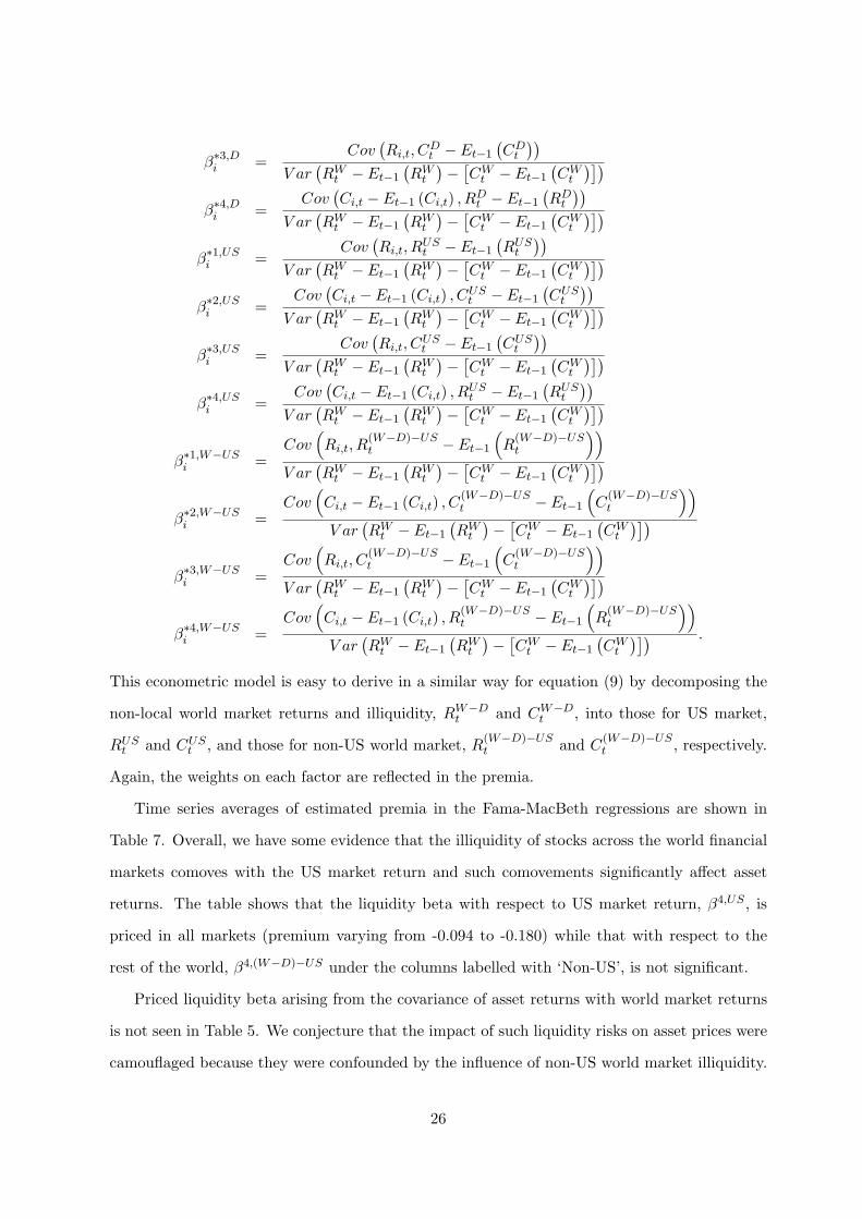
This econometric model is easy to derive in a similar way for equation (9) by decomposing the

non-local world market returns and illiquidity, RW−Dt and CW−D

t , into those for US market,

RUSt and CUS

t , and those for non-US world market, R(W−D)−USt and C

(W−D)−USt , respectively.

Again, the weights on each factor are reflected in the premia.

Time series averages of estimated premia in the Fama-MacBeth regressions are shown in

Table 7. Overall, we have some evidence that the illiquidity of stocks across the world financial

markets comoves with the US market return and such comovements significantly affect asset

returns. The table shows that the liquidity beta with respect to US market return, β4,US , is

priced in all markets (premium varying from -0.094 to -0.180) while that with respect to the

rest of the world, β4,(W−D)−US under the columns labelled with ‘Non-US’, is not significant.

Priced liquidity beta arising from the covariance of asset returns with world market returns

is not seen in Table 5. We conjecture that the impact of such liquidity risks on asset prices were

camouflaged because they were confounded by the influence of non-US world market illiquidity.

26

Separating out the US market illiquidity makes the effect of US market illiquidity on asset price

clearer by removing such a confounding effect.

Table 7 also shows that the liquidity net beta with respect to the US market is priced in

developed markets (premium of 0.065 with t-value of 2.02). Liquidity net beta with respect to

non-US world market factors is priced in the emerging markets but not in the developed markets.

Examining each component of the liquidity net beta reveals that the pricing of liquidity net beta

is mostly driven by β4,US in developed markets. In contrast, liquidity net beta effect is driven

by the commonality beta, β2,(W−D)−US , in the emerging markets. The commonality beta is

marginally priced in the overall world markets with a premium of 0.243.

The evidence in this subsection shows that US market returns affect asset prices of individual

stocks from around the world through covariance of illiquidity with US market return. When

the US market is in a downturn, global investors need to re-balance their portfolios. In such

re-balancing, stocks whose liquidity plummets in a US market downturn is less valuable. Finally,

investors request compensation to hold such stocks and the asset price is negatively related to

such liquidity risk.

6.6 Time series tests

Until now, we have presented the results of cross-sectional regressions in a Fama-MacBeth frame-

work. Another popular method of showing the importance of liquidity risks in asset pricing is

a time-series tests (Pastor and Stambaugh (2003), Sadka (2004) and Liang and Wei (2005)).

The time-series test does not directly test the LCAPM since it does not jointly test the multiple

risks in the model. Thus, the time-series test results should be evaluated as supporting evidence

confirming the pricing of risk factors, not as evidence in favor of or against a particular asset

pricing model. Since our Fama-MacBeth regression tests show that the risks related to global

markets are more important than those related to local markets, we perform time-series tests

based on predicted betas with respect to world market returns and illiquidity only. Predicted

global betas are obtained by the econometric model of (11).

Results from the three different restrictions on j in equation (11) are reported in panel A

of Table 8, each labelled with ‘All countries’, ‘Developed markets’ and ‘Emerging markets’:

In the rows labelled with ‘All countries’, stocks are sorted into ten equally-weighted portfolios

27

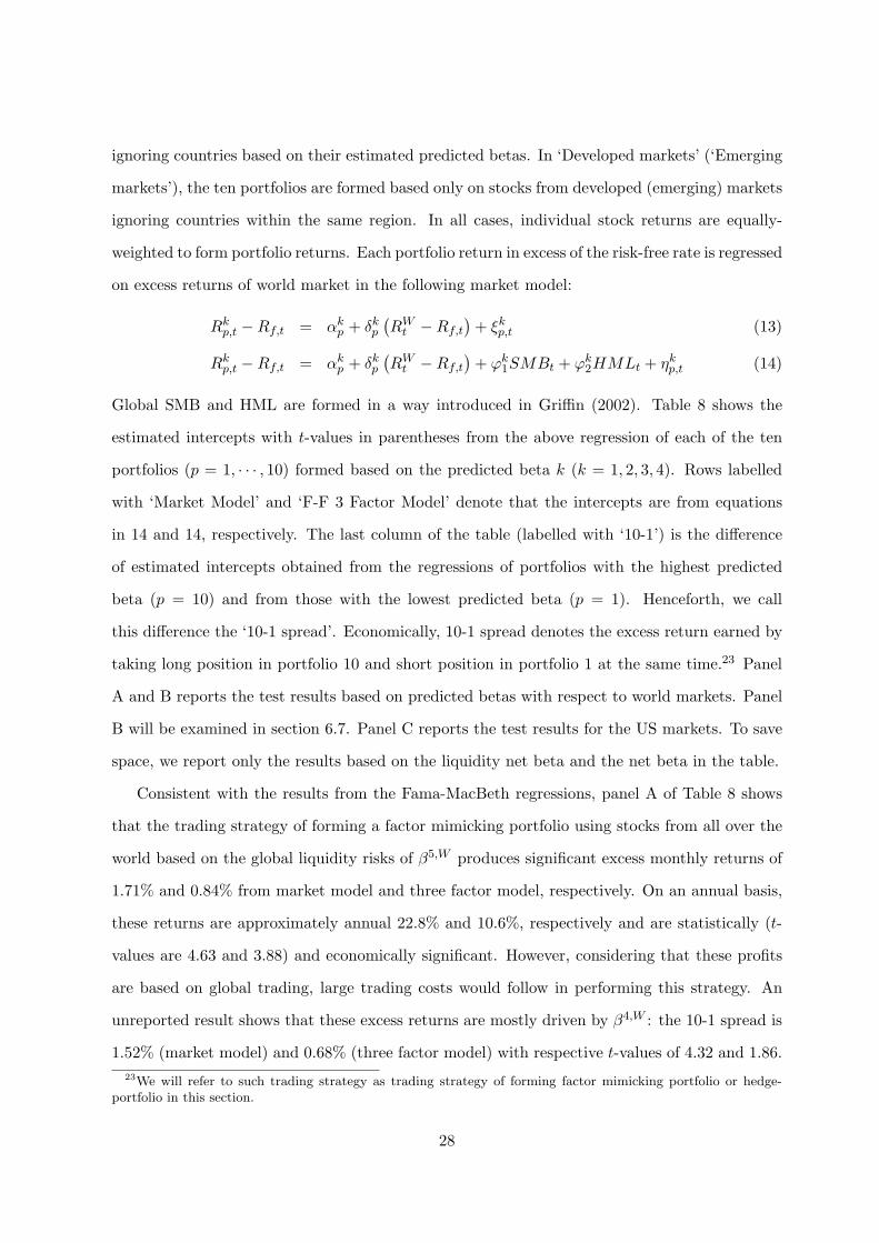
ignoring countries based on their estimated predicted betas. In ‘Developed markets’ (‘Emerging

markets’), the ten portfolios are formed based only on stocks from developed (emerging) markets

ignoring countries within the same region. In all cases, individual stock returns are equally-

weighted to form portfolio returns. Each portfolio return in excess of the risk-free rate is regressed

on excess returns of world market in the following market model:

Rkp,t −Rf,t = αk

p + δkp

(RW

t −Rf,t

)+ ξk

p,t (13)

Rkp,t −Rf,t = αk

p + δkp

(RW

t −Rf,t

)+ ϕk

1SMBt + ϕk2HMLt + ηk

p,t (14)

Global SMB and HML are formed in a way introduced in Griffin (2002). Table 8 shows the

estimated intercepts with t-values in parentheses from the above regression of each of the ten

portfolios (p = 1, · · · , 10) formed based on the predicted beta k (k = 1, 2, 3, 4). Rows labelled

with ‘Market Model’ and ‘F-F 3 Factor Model’ denote that the intercepts are from equations

in 14 and 14, respectively. The last column of the table (labelled with ‘10-1’) is the difference

of estimated intercepts obtained from the regressions of portfolios with the highest predicted

beta (p = 10) and from those with the lowest predicted beta (p = 1). Henceforth, we call

this difference the ‘10-1 spread’. Economically, 10-1 spread denotes the excess return earned by

taking long position in portfolio 10 and short position in portfolio 1 at the same time.23 Panel

A and B reports the test results based on predicted betas with respect to world markets. Panel

B will be examined in section 6.7. Panel C reports the test results for the US markets. To save

space, we report only the results based on the liquidity net beta and the net beta in the table.

Consistent with the results from the Fama-MacBeth regressions, panel A of Table 8 shows

that the trading strategy of forming a factor mimicking portfolio using stocks from all over the

world based on the global liquidity risks of β5,W produces significant excess monthly returns of

1.71% and 0.84% from market model and three factor model, respectively. On an annual basis,

these returns are approximately annual 22.8% and 10.6%, respectively and are statistically (t-

values are 4.63 and 3.88) and economically significant. However, considering that these profits

are based on global trading, large trading costs would follow in performing this strategy. An

unreported result shows that these excess returns are mostly driven by β4,W : the 10-1 spread is

1.52% (market model) and 0.68% (three factor model) with respective t-values of 4.32 and 1.86.23We will refer to such trading strategy as trading strategy of forming factor mimicking portfolio or hedge-

portfolio in this section.

28

While trading based on global liquidity net beta produces significant excess returns, similar

trading based on net beta including market risk, β6,W , does not produce any significant profits.

In either the market model or the three factor model, we see that the 10-1 spread is statistically

insignificant.

Panel A of Figure 2 plots intercepts from the market model for global liquidity net beta

(Panel A of Table 8). Bars in the graph denote excess returns while lines with bullets are for

matching t-values. The last columns of the graph (shaded area) denotes 10-1 spread. The graph

clearly shows that monotonically increasing pattern of intercepts according to size of global

liquidity net beta in overall, developed, and emerging markets. It also shows that excess returns

based on global liquidity net beta are largest in emerging markets.

Panel C shows the time-series test results for US stocks. Every stock in the US market is

sorted into 10 portfolios based on predicted betas estimated with respect to the US local market

returns and illiquidity (rows labelled with ‘US local’) or with respect to those of world market

(‘US world’). Local predicted betas are based on the fully-segmented world financial market

model of (2) while the global predicted betas are obtained from the fully-integrated model of

(4).

The liquidity net betas with respect to both local and world market factors are strongly

priced in the US market. The trading strategy of buying high liquidity net beta stocks and

selling low ones in the US market produces excess returns of 1.48% and 1.32%, respectively

for the local and global market betas (three factor model). These correspond to annual excess

returns of 19.43% and 17.16%, respectively. In contrast to Fama-MacBeth regression results for

US market in Table 4, trading based on β2,D and β3,D in US market also produces significant

profits (unreported). In a three factor model, 10-1 spread based on β2,D (β3,D) produces 1.08%

(0.58%) excess returns. In a market model, the spread is 0.95% and 0.80% for β2,D and β3,D,

respectively, or 12.07% and 10.07% annually.24 However, a similar trading strategy based on

the net beta, β6,D, does not produce significant excess returns in the US market. Panel B of

Figure 2 plots intercepts from market model for local and global liquidity net beta for US stocks

(Panel C of Table 8).24Pastor and Stambaugh (2003) find annual 8.23% excess returns in a market model regression using equally-

weighted portfolios based on β3,D.

29

In this section, we find confirming evidence of the empirical results from the Fama-MacBeth

regression tests in the previous subsections. In addition, we find that the trading strategy of

forming hedge-portfolios based on global liquidity risks produces economically significant excess

returns.

6.7 Subperiod analysis

In the previous sections, we saw that global liquidity risks are more important than local market

illiquidity. We expect that the global effect would be stronger in recent years as the financial

globalization process has evolved.25 Bekaert and Harvey (2000) and Henry (2000), among others,

suggest the specific dates of financial globalization before and after which, 12 to 20 emerging

markets have structural breaks in the equity returns, cost of capital, volatility of returns, market

risk or the correlation with global market returns. According to their research,26 most countries

in our sample have liberalization dates in the period between 1986 and 1992. However, splitting

the sample period based on these financial globalization date would make the tests based on

different samples of stocks. In Table 1, we see that many emerging markets begin to have data

in late 1980s to mid-1990’s. In addition, estimating pre-ranking betas requires the stocks to

have five years data before they begin to have pre-ranking betas. Thus, stocks whose data start

in the mid-1990’s can be included in the Fama-MacBeth regression only from the late 1990’s.

Instead of splitting the sample periods based on financial liberalization dates, we focus on

the event of the Long-Term Capital Management (LTCM) crisis. It is interesting to see the

difference, if any, in the pricing of liquidity risks pre- and post-LTCM crisis (January 1989

- August 1998 and September 1998 - December 2004, respectively) since the LTCM event is

known to have led to a deterioration in liquidity in international financial markets and in the

post-LTCM period, liquidity has improved rather quickly in many countries.27

Table 9 shows the results from the Fama-MacBeth regression tests using predicted betas with

respect to world market factors based on the model of fully-integrated world financial markets25Bekaert, Harvey, and Lundblad (2003) find the evidence that supports this hypothesis.26See Table I of Bekaert and Harvey (2000) and Table II of Henry (2000).27“It was felt that liquidity pre-LTCM in many markets was underpriced, and that this led financial institutions

to underestimate liquidity risks”, “Most of the indicators ... show that liquidity has since [fall of 1998] improved,sometimes significantly, across a large cross-section of markets, with the notable exception of the US governmentbond market.” (Structural Aspects of Market Liquidity from a Financial Stability Perspective, Committee on theGlobal Financial System, June (2001), Bank for International Settlements)

30

of (4) for the period of January 1994 - August 1998 (panel A) and September 1998 - December

2004 (panel B). Global liquidity net beta β5,W is priced both in the pre- and post-LTCM period

in all markets. The magnitude of the premium is larger in the pre-LTCM period (0.17) than

in post-LTCM period (0.11) in overall world market. However, the magnitude of the premium

is larger in the post-LTCM period (0.207) than in the pre-LTCM period (0.156) in emerging

markets suggesting that the effect of world market integration on the pricing implication of

liquidity risks improves in the post-LTCM period in emerging markets.

The test results based on global commonality liquidity risks show sharp contrasts between

the two subperiods. We see that global commonality liquidity risks become significant in the

post-LTCM period. In the post-LTCM period, global commonality liquidity beta, β2,W , is priced

in all markets while it is never priced in pre-LTCM period. For example, in emerging markets,

commonality liquidity beta is not priced with a premium of -0.34 (t-value of -0.77) in the pre-

LTCM period. This becomes significant in post-LTCM period with a premium of 0.36 (t-value

of 1.95).

Subperiod analysis based on time-series tests in the panel B of Table 8 supports the inference

from Table 9. In panel B of Table 8, global betas are obtained in a fully-integrated world financial

market model of (4). In the post-LTCM period, the 10-1 spread based on the global liquidity

net beta is statistically and economically significant. In emerging markets, trading based on

global liquidity net beta produces higher excess returns in the post-LTCM period than in the

pre-LTCM period supporting evidence in Table 9. In the emerging markets, the spread is 3.80%

in the post-LTCM period and this excess return is larger than the 2.92% shown for the whole

sample period in panel A in the same table.

Results from subperiod analysis can be summarized as follows. First, we find that global

liquidity net beta is priced in both pre- and post-LTCM period. Second, the effect of global

liquidity net beta on assets in emerging markets is stronger in post-LTCM period than in pre-

LTCM period. Third, we find an increasing impact of global commonality liquidity risks on

asset price in overall world markets in post-LTCM period. These findings are consistent with

our conjecture that the importance of global liquidity risk increases over time with the degree

of financial integration.

31

7 Robustness tests

The goal of this section is to evaluate the robustness of the empirical results in the previous

section. In section 6, we used various test methods such as Fama-MacBeth regressions based on

predicted betas, time-series tests and subperiod analysis. Consistent results produced by each

test show the robustness of our empirical results. In this section, we show that the previous

results are not specific to the method of constructing innovations in returns and illiquidity. We

also show the test results based on standard two-way sorts in Fama-MacBeth regressions of

Fama and French (1992) based on post-ranking betas.

7.1 Different innovation

At the cost of having look-ahead bias and employing discontinuous time-series (see section 5.1),

we test the LCAPM based on innovations from AR(2) methods following Pastor and Stambaugh

(2003) and Acharya and Pedersen (2005). Based on predicted betas, we also test whether the

innovations from an AR(1) fitting produce similar results and find virtually no difference for our

inference about the priced liquidity risks in the previous section.28

Using an AR(2) fitting, we also find that global liquidity risk is more important than local

liquidity risk and that global liquidity risk arising from the covariance of stock illiquidity with

market return, β4,W is priced in the world financial markets. We also find that US market is an

important driving force of world market illiquidity. Employing an AR(1) instead of an AR(2)

and including time-trend in AR fitting does not make significant difference in the inference.29

7.2 Two-way sorts

In the Fama-MacBeth regression tests of Fama and French (1992), post-ranking betas are es-

timated by the portfolios formed based on size and estimated pre-ranking betas (2-way sorts).

Size is a popular instrument for sorting stocks because portfolios sorted based on size generally

help produce sufficient dispersion in estimated loadings, and, in turn, such dispersion increases

the power of the test. This might be controversial in that it may artificially infuse a size effect

into the test. However, since the two-way sorts have been widely used in the previous studies in28Thus, the result is not tabulated. It is available upon request from the author.29Actually, previous version of this paper is based on AR(2) fitting throughout. Readers may refer to the tables

in the previous version of this paper. It is available upon request.

32

asset pricing, as a robustness check, we report the Fama-MacBeth regression results from post-

ranking betas estimated by portfolios from two-way sorts. For comparison with other studies

which employ AR(2) fitting to construct innovations in returns and illiquidity, we follow AR(2)

fitting in this two-way sorts exercise. Overall, the two-way sort does not change the previous

results about the global liquidity risk of β4,W .

In two-way sorts, stocks are first sorted into N (N = 3, 5, 10) size portfolios based on the

market capitalization (in US dollar terms) at the beginning of each year. Then, within each

size group, stocks are re-sorted into N portfolios by their estimated pre-ranking betas, which

are estimated as described in section 5.2. If the number of stocks in a country is between 100

(inclusive) and 300, the stocks are sorted into 3 × 3 portfolios (small country-size group). N = 5

for each country who covers more than 300 and less than 500 stocks (medium country-size group)

and N = 10 for countries with more than 500 stocks (large country-size group).30 Similarly,

stocks are sorted into portfolios based on their size and pre-ranking betas with respect to world

market returns and illiquidity.

As in Fama and French (1992), post-ranking betas are calculated using portfolio returns

and innovations in illiquidity for the entire time-series: Post-ranking beta k is calculated by the

definition of beta k under the equation (2) or (4), respectively, with respect to local and world

market factors using returns and innovations in illiquidity of portfolio formed based on local or

world pre-ranking beta k. These post-ranking betas for each portfolio are assigned to individual

stocks which belong to that portfolio. As a result, each individual stock has a market beta as

well as three liquidity betas for both local and world market factors which are assigned from

different portfolios that it belongs to.

Appendix 3 reports the result of Fama-MacBeth regression tests for individual stocks with

two-way sorted post-ranking betas with respect to local market (panel A) and world mar-

ket factors (panel B) for the period of 1988-2004. Local risks are based on the LCAPM of

fully-segmented world markets while the global risks are obtained based on the model of fully-

integrated world financial markets.30Stocks from countries of Austria, Belgium, Chile, Denmark, Finland, Indonesia, Israel, Mexico, Netherland,

New Zealand, Norway, Philippines, Poland, Portugal, Spain and Turkey are sorted into three portfolios. The fiveportfolio groups for each beta are formed for the countries of Greece, India, Italy, Singapore, Sweden, Switzerlandand Thailand. The ten portfolio group is for the countries of Australia, Canada, China, France, Germany, HongKong, Japan, Malaysia, South Africa, South Korea, Taiwan, the UK and the US.

33

We see that two-way sorts do not change the inference about global liquidity risk of β4,W .

Consistent with our previous results, it is priced in developed markets and the overall world

markets. The average premium varies from 0.027 to 0.057 with absolute t-values of 1.95 and

3.18 in developed markets. In the overall world markets, the absolute values of the premiums

are 0.025 to 0.050 with absolute t-values of 1.69 to 3.19 when the firm characteristics are not

controlled for. This global liquidity risk is also priced in the US market together with β3,W and

local liquidity risks of β3,D and β4,D. We note that the commonality beta with respect to both

local and world markets continuously have the wrong sign.

In developed markets, β3,W is priced in the specifications without size and book-to-market.

However, this is not strong enough to lead β3,W to be priced in the overall world markets. Dif-

ferent from our previous results, local liquidity risk of β4,D is now priced in developed markets

(premiums of -0.057 with absolute t-values of larger than 2) in the specifications without firm

characteristics. This significant result for β4,D in developed markets contributes to the signifi-

cance of the same liquidity risk in the overall world markets. In emerging markets, β3,D is no

longer priced in any presented specification.

8 Conclusion

This paper investigates an equilibrium asset pricing relationship with liquidity both as a char-

acteristic and as a risk factor in international financial markets. Our test assets cover 25,000

stocks from 48 countries from emerging and developed markets for January 1988 to December

2004. To our knowledge, this is the first paper that assesses multiple liquidity risks as well as

market risk similar to Acharya and Pedersen (2005)’s liquidity-adjusted capital asset pricing

model (LCAPM) for international financial markets. It is also the most comprehensive to date,

in that our sample covers stocks from both emerging and developed markets, which helps form

truly representative world market factors.

Using a variety of test methods including Fama-MacBeth cross-sectional tests, and in the

time-series tests, we evaluate the unconditional version of the LCAPM extended to the inter-

national financial markets. Though we reject the overidentifying restrictions of the LCAPM

of Acharya and Pedersen (2005), we find that a variety of liquidity risks arising from the co-

variances of asset return (liquidity) with local and global market liquidity (returns) are priced.

34

Interestingly, we find global liquidity risks subsume local liquidity risks and a trading strategy

based on non-traded global liquidity risks is shown to produce annualized excess returns of 10.6

percent. We interpret our evidence as consistent with an intertemporal capital asset pricing

model (Merton (1973)) in which stochastic shocks to global liquidity serve as a priced state

variable.

In this paper, we show that the US market is an important driving force of global liquidity

risks. Specifically, the US market returns affect asset prices of individual stocks from around the

world through covariances of liquidity with US market returns. When the US market declines,

global investors seek to re-balance their portfolios. In the process of this re-balancing, stocks

whose liquidity plummets in a US market downturn are less valuable. Finally, investors require

compensation to hold such stocks and the asset price is negatively related to such liquidity risk.

An important limitation is that we have tested only the unconditional version of the global

LCAPM. An interesting extension of this study will be to test the conditional version of the

LCAPM, where liquidity risks vary over time in a way that depend on predetermined information

variables. Such an extension will also allow us to investigate the determinants of time-varying

liquidity risk premia in international financial markets. Based on the results in this paper, we

conjecture that the economic variables that have been revealed to affect US market returns

would also influence time-varying liquidity risks in world financial markets.

35

References

Acharya, V., and L. H. Pedersen, 2005, Asset pricing with liquidity risk, Journal of Financial

Economics 77, 375–410 forthcoming.

Amihud, Y., 2002, Illiquidity and stock returns: Cross-section and time-series effects, Journal

of Financial Markets 5, 31–56.

, and H. Mendelson, 1986, Asset pricing and the bid-ask spread, Journal of Financial

Economics 17, 223–249.

Bekaert, G., and C. R. Harvey, 2000, Foreign speculators and emerging equity markets, Journal

of Finance 55, 565–613.

, and C. Lundblad, 2003, Liquidity and expected returns: Lessons from emerging mar-

kets, working paper.

Black, F., M. Jensen, and M. Scholes, 1972, The Capital Asset Pricing Model: Some Empirical

Tests, Studies in the Theory of Capital Markets (Praeger).

Brennan, M. J., and A. Subrahmanyam, 1996, Market microstructure and asset pricing: On the

compensation for illiquidity in stock returns, Journal of Financial Economics 41, 441–464.

CGFS, 2001, Structural aspects of market liquidity from a financial stability perspective, Com-

mitte on the Global Financial System, Bank for International Settlement.

Chordia, T., R. Roll, and A. Subrahmanyam, 2000, Commonality in liquidity, Journal of Fi-

nancial Economics 56, 3–27.

Chordia, T., L. Shivakumar, and A. Subrahmanyam, 2004, Liquidity dynamics across small and

large firms, Economic Notes 33, 111–143.

Coughenour, J. F., and M. M. Saad, 2004, Common market makers and commonality in liquidity,

Journal of Financial Economics 73, 37–69.

De Long, J. B., A. Shleifer, L. H. Summers, and R. J. Waldmann, 1990, Noise trader risk in

financial markets, Journal of Political Economy 98, 703–738.

36

Domowitz, I. H., and X. Wang, 2002, Liquidity, liquidity commonality and its impact on portfolio

theory, Working Paper.

Errunza, V., and E. Losq, 1985, International asset pricing under mild segmentation: Theory

and test, Journal of Finance XL, 105–124.

Fama, E. F., and K. R. French, 1992, The cross-section of expected stock returns, Journal of

Finance 47, 427–465.

Glosten, L. R., and P. R. Milgrom, 1985, Bid, ask and transaction prices in a specialist market

with heterogenously informed traders, Journal of Financial Economics 14, 71–100.

Griffin, J., 2002, Are the fama and french factors global or country-specific?, Review of Financial

Studies 15, 783–803.

Grossman, S. J., and M. H. Miller, 1988, Liquidity and market structure, Journal of Finance

43, 617–633.

Harford, J., and A. Kaul, 2004, Correlated order flow: Pervasiveness, sources, and pricing effects,

Journal of Financial and Quantitative Analysis.

Harvey, C. R., 1991, The world price of covariance risk, Journal of Finance pp. 111–157.

, 1995, Predictable risk and returns in emerging markets, Review of Financial Studies 8,

773–816.

Hasbrouck, J., 2005, Trading costs and returns for us equities: The evidence from daily data,

Working paper.

, and D. J. Seppi, 2001, Common factors in prices, order flows, and liquidity, Journal of

Financial Economics 59, 383–411.

Henry, P. B., 2000, Stock market liberalization, economic reform, and emerging market equity

prices, Journal of Finance 55, 529–564.

Ho, T., and H. Stoll, 1981, Optimal dealer pricing under transaction and return uncertainty,

Journal of Financial Economics 9, 47–73.

37

Holthausen, R., R. Leftwich, and D. Mayers, 1991, Large block transactions, the speed of re-

sponse and temporary and permanent stock price impacts, Journal of Financial Economics

26, 71–95.

Huberman, G., and D. Halka, 2001, Systematic liquidity, Journal of Financial Research 24.

Ince, O., and R. B. Porter, 2003, Individual equity return data from thomson datastream:

Handle with care!, University of Florida working paper.

Jones, C., 2002, A century of stock market liquidity and trading costs, working paper.

Kang, J-K, and R. M. Stulz, 1997, Why is there a home bias? an analysis of foreign portfolio

equity ownership in japan, Journal of Financial Economics 46, 3–28.

Karolyi, G. A., 1992, Predicting risk: some new generalizations, Management Science 38, 57–74.

, and R. M. Stulz, 2002, Are financial assets priced locally or globally?, NBER working

paper.

Keim, D., 2003, The cost of trend chasing and the illusion of momentum profits, Working Paper,

University of Pennsylvania.

Korajczyk, R. A., and R. Sadka, 2005, Are momentum profits robust to trading costs?, Journal

of Finance forthcoming.

Kyle, A. S., 1985, Continuous auctions and insider trading, Econometrica 53, 1315–1335.

Lee, K-H., 2005, Liquidity spillovers, Doctoral dissertation, The Ohio State University.

Lesmond, D. A., 2005, Liquidity of emerging markets, Journal of Financial Economics forth-

coming.

, J. P. Ogden, and C. A. Trzcinka, 1999, A new estimate of transaction costs, Review of

Financial Studies 12, 1113–1141.

Lesmond, D. A., M. J. Schill, and C. Zhou, 2004, The illusory nature of momentum profits,

Journal of Financial Economics 71, 349–380.

38

Liang, Samuel X., and J. K-C Wei, 2005, Global liquidity risk, Hong Kong University of Science

and Technology.

Merton, R., 1973, An intertemporal capital asset pricing model, Econometrica 41, 867–887.

Pastor, L., and R. F. Stambaugh, 2003, Liquidity risk and expected stock returns, Journal of

Political Economy 111, 642–685.

Roll, R., 1984, A simple implicit measure of the effective bid-ask spread in an efficient market,

Journal of Finance 39, 1127–1139.

Rouwenhorst, K. G., 1999, Local return factors and turnover in emerging stock markets, Journal

of Finance pp. 1439–1464.

Sadka, R., 2004, Liquidity risk and asset pricing, Working Paper, University of Washington.

Spiegel, M., and X. Wang, 2005, Cross-sectional variation in stock returns: Liquidity and idio-

syncratic risk, working paper.

Stahel, C. W., 2004a, Are liquidity shocks correlated across equity markets?, Doctoral disserta-

tion, The Ohio State University.

, 2004b, Is there a global liquidity factor?, Doctoral dissertation, The Ohio State Uni-

versity.

Stoll, H, 1978, The supply of dealer services in securities markets, Journal of Finance 33, 1133–

1151.

Stulz, R. M., 2005, The limits of financial globalization, Journal of Finance 60, 1595–1638.

Tesar, Linda L., and I. M. Werner, 1995, Home bias and high turnover, The Journal of Inter-

national Money and Finance 14, 467–492.

Vasicek, O., 1973, A note on using cross-sectional information in bayesian estimation of security

betas, Journal of Finance 28, 1233–1239.

39

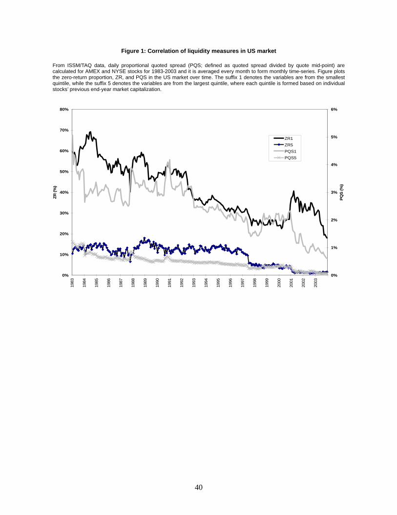
40

Figure 1: Correlation of liquidity measures in US market From ISSM/TAQ data, daily proportional quoted spread (PQS; defined as quoted spread divided by quote mid-point) are calculated for AMEX and NYSE stocks for 1983-2003 and it is averaged every month to form monthly time-series. Figure plots the zero-return proportion, ZR, and PQS in the US market over time. The suffix 1 denotes the variables are from the smallest quintile, while the suffix 5 denotes the variables are from the largest quintile, where each quintile is formed based on individual stocks’ previous end-year market capitalization.

0%

10%

20%

30%

40%

50%

60%

70%

80%

1983

1984

1985

1986

1987

1988

1989

1990

1991

1992

1993

1994

1995

1996

1997

1998

1999

2000

2001

2002

2003

ZR (%

)

0%

1%

2%

3%

4%

5%

6%

PQS

(%)

ZR1ZR5PQS1PQS5

41

Figure 2: Alphas

Panel A and B plots intercepts and t-values from market model of panel A and C of Table 8. Bar denote intercept while bulleted lines are for t-values.

Panel A: Alphas from market model for portfolios based on global liquidity risks

Alphas from market model for portfolios based on global liquidity risks

-1.50

-1.00

-0.50

0.00

0.50

1.00

1.50

2.00

2.50

3.00

3.50

1(small)

2 3 4 5 6 7 8 9 10 (big) 10-1

global liquidity net beta

alph

a (%

)

-3.00

-2.00

-1.00

0.00

1.00

2.00

3.00

4.00

5.00

t-val

ue

alpha (all) alpha (developed) alpha (emerging) t (all) t (developed) t (emerging)

Panel B: Alphas from market model for US portfolios based on US local and global liquidity risks

Alphas from market model for US portfolios based on US local and global liquidity risks

0.00

0.50

1.00

1.50

2.00

2.50

1 (small) 2 3 4 5 6 7 8 9 10 (big) 10-1

US local / global liquidity risks

alph

a (%

)

0.00

1.00

2.00

3.00

4.00

5.00

6.00

7.00

t-val

ue

alpha (US local) alpha (US world) t (local) t (world)

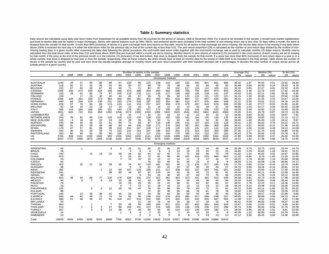
42

Table 1: Summary statistics Daily returns are calculated using daily total return index from Datastream for all available stocks from 48 countries for the period of January 1988 to December 2004. For a stock to be included in the sample, it should have market capitalization and book-to-market data and be traded in major exchanges. Stocks with special features such as DRs, REITs, and preferred stocks were excluded. If the total number of non-missing return day is less than 15 days within a month, the stock is dropped from the sample for that month. If more than 90% (inclusive) of stocks in a given exchange have zero returns on that date, returns for all stocks in that exchange are set to missing. We set the daily return to be missing if any daily return above 100% is reversed the next day or if either the total return index for the previous day or that of the current day is less than 0.01. The zero-return proportion (ZR) is calculated as the number of zero-return days divided by the number of non-missing trading days in a given month. After screening the daily data following the above procedure, the end-month total return index together with the end-month exchange rate is used to calculate monthly US dollar returns. Monthly returns calculated from the total return index of less than 0.01 and those above 300% that are reversed within a month are set to missing. Monthly returns or zero-returns of extreme 0.1% (inclusive) in the cross-section of each country are set to missing for that month. If the price at the end of the previous month is in the extreme 1% (inclusive) of top and bottom, that stock is dropped from the sample for that month. If a stock has more than 80% (inclusive) of zero-return days in a year or in a whole sample, that stock is dropped for that year or from the sample, respectively. After all these screens, the stock should have at least 12 months data for the period of 1988-2004 to be included in the final sample. Table shows the number of stocks in the sample by country and by year and also show the equally-weighted average of monthly return and zero return proportion with their standard deviation (all in percentage). N denotes the total number of unique stocks across all sample period in a given country.

N 1988 1989 1990 1991 1992 1993 1994 1995 1996 1997 1998 1999 2000 2001 2002 2003 2004 ZR return ZR return ZR return

AUSTRALIA 1140 29 57 85 96 98 97 100 99 125 158 154 182 235 395 801 841 865 38.50 1.97 35.00 0.51 22.62 18.39AUSTRIA 118 31 37 42 46 52 55 60 57 59 79 76 68 64 61 59 55 50 31.48 0.66 25.00 0.14 23.23 8.78BELGIUM 155 57 63 66 67 65 65 71 71 80 87 94 102 117 116 112 105 101 32.04 0.95 27.27 0.61 22.32 8.25CANADA 1308 250 274 299 324 338 348 372 388 429 450 464 596 756 794 834 874 820 25.46 1.45 22.73 0.47 17.62 15.32DENMARK 226 28 62 84 79 97 105 119 126 111 149 127 148 169 146 118 131 147 43.63 1.05 42.11 0.60 25.36 9.35FINLAND 159 17 26 30 40 44 45 57 55 75 85 94 120 124 121 122 121 34.15 1.18 30.00 0.41 22.66 11.84FRANCE 1058 109 161 338 373 384 392 391 392 402 499 561 630 680 727 697 635 591 28.41 1.05 21.05 0.31 22.87 13.09GERMANY 840 84 204 224 239 231 243 274 268 287 332 354 382 516 677 676 604 546 31.21 0.30 23.81 -0.21 24.28 14.25HONG KONG 828 57 76 83 89 113 133 131 153 257 347 358 379 379 497 618 678 698 32.99 1.40 27.27 -0.04 22.85 19.45IRELAND 52 14 19 22 19 14 15 14 15 11 16 12 15 13 16 18 21 23 48.96 1.04 52.17 0.53 22.92 12.08ITALY 366 143 166 184 186 191 190 178 161 157 172 185 200 215 243 235 232 218 16.59 0.48 10.00 -0.10 15.69 10.05JAPAN 1831 620 722 816 954 1202 1256 1274 1300 1353 1394 1400 1520 1542 1552 1601 1624 1583 23.45 0.41 15.79 -0.67 19.70 12.46LUXEMBOURG 23 8 10 7 10 13 14 13 12 13 16 15 13 34.65 0.82 31.82 0.53 19.57 7.81NETHERLANDS 240 78 92 95 116 126 128 133 139 138 153 165 183 182 164 145 140 135 26.46 0.99 19.05 0.62 21.14 10.17NEW ZEALAND 126 4 18 18 22 23 28 29 39 45 50 51 60 64 69 92 91 89 36.80 1.69 35.00 1.33 19.12 9.67NORWAY 245 38 46 49 53 51 66 71 83 87 110 135 155 141 127 124 126 128 35.41 1.25 30.00 0.70 24.22 13.71SINGAPORE 389 31 35 39 48 68 84 84 106 158 171 176 183 187 252 285 300 309 34.41 0.91 30.00 -0.12 21.36 14.43SPAIN 178 47 57 81 89 98 102 104 107 109 117 129 129 129 131 131 122 116 22.03 1.03 15.00 0.49 19.13 10.08SWEDEN 444 30 53 53 59 75 122 141 154 157 188 223 254 273 313 310 300 280 27.20 1.17 21.74 0.42 19.89 14.50SWITZERLAND 293 80 90 93 95 90 106 111 113 127 150 166 178 189 214 210 207 192 35.43 0.76 30.00 0.43 23.76 9.37UK 2765 848 1151 1169 1006 990 1006 1052 1032 1141 1356 1426 1388 1362 1400 1392 1364 1320 47.89 0.99 50.00 0.37 25.40 12.93US 6347 1757 1896 1870 1888 2136 2348 2637 3446 3782 4219 4391 4498 4429 4094 3865 3829 3637 20.22 1.62 17.39 0.68 14.75 13.95

ARGENTINA 64 1 3 9 15 21 26 32 40 39 42 32 44 49 49 30.39 0.74 22.73 -0.02 23.44 14.74BRAZIL 28 5 5 6 8 9 13 19 23 20 22 23 34.95 2.25 30.00 1.43 24.91 15.21CHILE 100 12 18 25 35 46 54 54 62 55 71 75 68 66 70 70 41.82 1.54 40.00 0.52 24.67 10.80CHINA 972 5 20 25 72 81 90 89 191 218 223 960 957 11.32 -0.86 8.70 -1.83 11.20 12.00COLOMBIA 23 7 10 10 10 12 12 14 11 9 12 16 17 46.22 1.78 45.00 1.14 20.68 10.89CZECH 64 16 53 60 51 34 23 6 8 9 38.59 -1.14 32.58 -1.45 26.56 14.17GREECE 322 25 27 31 29 55 74 97 110 161 161 59 72 276 277 163 130 17.79 0.66 13.64 -0.44 15.79 14.83HUNGARY 38 5 5 11 20 21 24 37 35 32 29 27 24.75 0.95 18.18 -0.10 20.81 12.10INDIA 302 1 15 59 107 119 189 211 217 208 222 237 264 241 201 20.82 0.21 15.00 -1.19 17.68 15.46INDONESIA 181 38 50 44 52 97 120 43 65 76 60 72 81 91 44.04 0.74 42.11 -0.30 22.58 16.38ISRAEL 88 6 20 24 36 45 47 60 72 75 65 20.65 0.90 11.76 0.25 20.12 10.99MALAYSIA 603 46 54 66 77 120 176 186 191 274 322 361 364 373 431 481 513 536 26.69 0.81 22.73 -0.40 17.98 16.59MEXICO 94 6 7 6 13 22 36 42 43 50 50 54 54 44 38 42 50 33.34 0.63 23.81 0.05 25.46 14.56PAKISTAN 79 16 25 29 25 24 41 48 51 60 62 65 67 30.51 1.76 22.22 0.21 24.36 14.63PERU 33 3 7 13 11 19 16 13 13 13 13 12 19 44.14 0.14 43.48 -0.40 23.38 13.22PHILIPPINES 131 2 4 12 25 30 40 76 90 88 90 79 83 72 71 81 44.72 0.05 42.11 -1.65 22.35 20.22POLAND 96 17 32 38 56 68 78 81 78 76 19.92 1.30 15.00 0.56 15.39 12.91PORTUGAL 100 23 38 38 43 45 54 55 56 66 66 58 59 50 49 45 45 32.26 0.47 28.57 -0.23 21.89 9.90S.AFRICA 505 44 42 49 71 70 74 92 90 136 153 176 329 356 317 284 248 237 40.85 1.04 38.89 0.55 24.23 15.47S.KOREA 689 21 46 59 67 81 109 157 216 244 280 275 355 531 542 555 567 554 12.08 1.07 9.52 -0.61 8.82 17.68SRI LANKA 23 11 16 15 16 15 18 17 18 12 9 40.41 0.09 40.00 -0.68 19.27 11.96TAIWAN 664 1 7 20 43 99 190 205 211 222 327 402 580 626 628 13.67 0.66 10.53 -0.51 9.40 14.93THAILAND 414 1 5 7 47 86 155 191 212 215 185 193 156 228 236 272 296 35.74 0.95 30.00 -0.59 22.75 20.28TURKEY 207 3 9 13 28 47 48 50 64 85 110 132 146 159 183 171 18.59 2.95 18.18 1.01 9.81 22.05VENEZUELA 14 1 4 6 7 10 6 7 10 10 10 9 8 40.49 1.22 40.00 -0.04 24.39 15.61ZIMBABWE 13 2 2 6 5 8 8 9 13 13 12 47.12 5.30 45.45 0.00 16.36 43.69

Total 24978 4446 5494 6005 6207 6998 7766 8563 9740 11050 12620 13109 13957 14835 15596 16199 16886 16410

Emerging markets

Average (%) Median (%) St dev (%)

Developed markets

Number of stocks in the sample

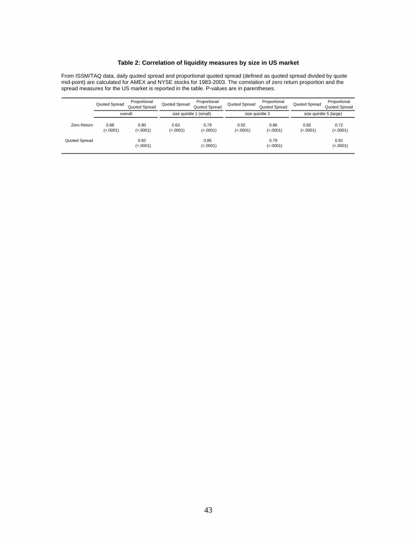
43

Table 2: Correlation of liquidity measures by size in US market

From ISSM/TAQ data, daily quoted spread and proportional quoted spread (defined as quoted spread divided by quote mid-point) are calculated for AMEX and NYSE stocks for 1983-2003. The correlation of zero return proportion and the spread measures for the US market is reported in the table. P-values are in parentheses.

Quoted Spread Proportional Quoted Spread Quoted Spread Proportional

Quoted Spread Quoted Spread Proportional Quoted Spread Quoted Spread Proportional

Quoted Spread

Zero Return 0.88 0.90 0.63 0.79 0.92 0.86 0.82 0.72 (<.0001) (<.0001) (<.0001) (<.0001) (<.0001) (<.0001) (<.0001) (<.0001)

Quoted Spread 0.92 0.85 0.79 0.91 (<.0001) (<.0001) (<.0001) (<.0001)

size quintile 3 size quintile 5 (large)overall size quintile 1 (small)

44

Table 3: Mean of portfolio formed based on predicted betas

For each individual stock, pre-ranking betas are estimated using the previous 5 years returns and illiquidity. The five-year window starts from January 1988 and is rolled forward at yearly intervals. To be included, stocks should have at least 36 monthy returns and innovations in illiquidity within the given window. Market returns and illiquidity are formed as a value-weight average of individual stocks' returns and illiquidity. Predicted beta is obtained by equation (7) using the coefficients estimated in equation (6). According to predicted betas, stocks are sorted into one of the following portfolios depending on the number of stocks for each country: If the number of stocks in a country is between 100 (inclusive) and 300, the stocks are sorted into 3 portfolios. We use 5 portfolios if the number of stocks in a country is between 300 and 500 and 10 portfolios if the number of stocks is greater than 500. Table reports the equally-weghted average across countries of time-series averages of each country for each variable according to predicted beta-based portfolio formed this way for the period of 1994-2004. Beta 1 to Beta 4 denote betas defined under equation (2) for panel A and (4) for panel B.

small 2 big small 2 big small 2 big small 2 bigreturn (%) 1.42 1.31 1.09 1.16 1.21 1.43 1.48 1.28 1.05 1.68 1.16 0.99

ZR (%) 34.91 33.79 30.07 30.35 32.95 35.32 32.49 33.09 33.17 33.67 32.93 32.18log(MV) 5.11 4.95 4.96 5.06 4.97 5.00 4.85 5.01 5.15 4.65 5.02 5.33log(B/M) -0.27 -0.22 -0.26 -0.28 -0.25 -0.22 -0.12 -0.25 -0.37 -0.03 -0.25 -0.46

predicted beta * 0.26 0.36 0.46 2.62 5.05 7.40 -3.69 -2.30 -0.92 -13.36 -9.84 -6.11

small 2 3 4 big small 2 3 4 big small 2 3 4 big small 2 3 4 bigreturn (%) 1.64 1.48 1.25 0.96 1.27 1.03 1.47 0.98 1.48 1.50 1.40 1.62 1.28 1.23 1.00 1.74 1.42 1.39 1.09 0.89

ZR (%) 30.27 28.65 27.91 25.92 24.88 22.75 25.09 27.27 28.43 33.45 28.74 27.26 27.75 26.76 27.13 28.40 28.11 26.93 26.92 27.29log(MV) 4.24 4.25 4.27 4.31 4.27 4.43 4.32 4.25 4.10 4.24 4.09 4.23 4.26 4.32 4.43 3.87 4.16 4.30 4.36 4.64log(B/M) -0.10 -0.01 0.00 0.05 -0.03 -0.06 0.03 0.00 0.03 -0.07 0.06 0.09 0.02 -0.05 -0.18 0.19 0.11 0.02 -0.08 -0.30

predicted beta * 0.16 0.25 0.31 0.37 0.47 2.05 4.14 5.23 6.40 8.13 -4.38 -3.23 -2.60 -1.87 -0.70 -14.98 -11.76 -10.06 -8.31 -4.87

small 3 5 7 10 (big) small 3 5 7 10 (big) small 3 5 7 10 (big) small 3 5 7 10 (big)return (%) 1.47 1.51 1.14 0.83 0.90 1.06 1.22 1.02 1.35 1.40 1.56 1.25 1.40 1.23 0.78 1.87 1.59 1.32 1.15 0.35

ZR (%) 28.24 28.46 27.02 26.18 22.47 23.22 25.13 25.76 26.69 30.45 25.31 25.95 26.35 27.21 26.29 27.81 26.81 26.07 26.62 25.36log(MV) 4.96 4.97 4.98 4.99 4.95 4.93 4.99 5.06 5.02 4.88 4.77 4.94 5.04 5.03 5.00 4.45 4.82 5.03 5.03 5.33log(B/M) -0.32 -0.18 -0.21 -0.19 -0.30 -0.34 -0.22 -0.24 -0.20 -0.14 -0.05 -0.11 -0.17 -0.24 -0.57 0.07 -0.10 -0.17 -0.25 -0.60

predicted beta * 0.18 0.31 0.37 0.42 0.59 1.45 3.80 4.83 5.89 8.60 -4.82 -3.31 -2.53 -1.89 0.15 -17.30 -13.23 -11.23 -9.08 -3.48

small 2 big small 2 big small 2 big small 2 bigreturn (%) 1.39 1.27 1.15 1.16 1.31 1.34 1.32 1.22 1.27 1.50 1.30 1.02

ZR (%) 33.82 34.08 30.82 31.34 33.18 34.16 32.08 33.13 33.52 33.24 32.89 32.62log(MV) 4.98 4.98 5.06 5.09 5.01 4.93 4.91 5.00 5.11 4.71 5.01 5.30log(B/M) -0.24 -0.24 -0.27 -0.30 -0.26 -0.20 -0.22 -0.21 -0.32 -0.09 -0.25 -0.40

predicted beta * 0.23 0.35 0.51 1.76 2.73 3.63 -5.38 -4.26 -3.25 -14.30 -8.46 -2.58

small 2 3 4 big small 2 3 4 big small 2 3 4 big small 2 3 4 bigreturn (%) 1.69 1.40 1.16 0.98 1.34 1.18 1.15 1.23 1.45 1.49 1.11 1.23 1.34 1.39 1.44 1.70 1.37 1.41 1.17 0.91

ZR (%) 28.96 28.71 27.59 27.73 24.46 24.33 24.99 27.93 28.15 31.64 26.70 27.16 27.86 27.60 28.29 28.81 27.28 27.44 26.19 27.90log(MV) 4.17 4.18 4.29 4.34 4.35 4.41 4.36 4.21 4.31 4.05 4.20 4.28 4.29 4.23 4.33 3.89 4.23 4.37 4.39 4.43log(B/M) -0.09 0.03 -0.02 -0.01 0.02 -0.07 -0.02 0.02 0.00 0.01 -0.04 0.07 0.02 -0.01 -0.11 0.17 0.09 -0.02 -0.03 -0.26

predicted beta * 0.14 0.25 0.33 0.40 0.54 1.58 2.39 3.03 3.51 4.42 -5.71 -4.65 -4.12 -3.41 -2.51 -16.68 -11.46 -8.60 -5.78 -0.34

small 3 5 7 10 (big) small 3 5 7 10 (big) small 3 5 7 10 (big) small 3 5 7 10 (big)return (%) 1.70 1.24 1.19 1.09 0.88 0.99 1.35 1.25 1.19 1.49 1.26 1.27 1.20 1.18 0.97 1.87 1.55 1.10 1.15 0.49

ZR (%) 26.84 27.67 27.36 26.23 23.38 24.56 25.84 26.50 26.99 28.12 24.66 25.92 26.69 27.38 26.01 26.92 26.30 26.84 27.33 25.54log(MV) 4.83 4.92 4.99 5.03 5.04 5.04 5.03 5.03 4.97 4.79 4.79 4.96 4.99 4.98 5.07 4.55 4.84 5.00 5.04 5.31log(B/M) -0.25 -0.16 -0.19 -0.20 -0.35 -0.38 -0.22 -0.22 -0.20 -0.11 -0.16 -0.15 -0.18 -0.21 -0.42 0.03 -0.11 -0.16 -0.24 -0.57

predicted beta * 0.14 0.30 0.37 0.44 0.67 1.11 2.24 2.68 3.07 4.34 -6.51 -5.24 -4.60 -4.13 -2.49 -20.16 -13.51 -10.30 -6.71 1.36

countries with number of stocks greater than 500

countries with number of stocks greater than 100 and less than 300Beta 1 Beta 2 Beta 3 Beta 4

countries with number of stocks greater than 100 and less than 300

countries with number of stocks greater than 300 and less than 500

countries with number of stocks greater than 500

panel A: predictied beta (LOCAL)

panel B: predicted beta (WORLD)Beta 1 Beta 2 Beta 3 Beta 4

countries with number of stocks greater than 300 and less than 500

45

Table 4: Fama-MacBeth regression by predicted betas (local market) Table reports the time-series averages of estimated premia from Fama-MacBeth regression based on the fully-segmented world market model of (2) using predicted betas with respect to local market factors for the period of 1994-2004. For each individual stock, pre-ranking betas are estimated using the previous 5 years returns and illiquidity. To be included, stocks should have at least 36 monthy returns and innovations in illiquidity within the given window. In calculating betas, innovations in liquidity are obtained by first differencing. Market returns and illiquidity are formed as a value-weight average of individual stocks' returns and illiquidity. Predicted beta of individual stock is obtained by equation (7) using the coefficients estimated in equation (6). ZR denotes the coefficient of expected illiquidity which is an average of illiquidity for the previous 12 month data (at least 6 months is required). MV and B/M are the previous year-end market capitalization and book-to-market ratio, respectively. Beta 1 to Beta 6 denote the premium for liquidity risks defined under equation (2) and (3). T-values are in parenthesis.

Intercept ZR Beta 1 Beta 2 Beta 3 Beta 4 Beta 5 Beta 6 log(MV) log(B/M)

All 0.009 -0.025countries (2.52) (-2.63)

-0.023 -0.001 -0.009 0.117(-3.05) (-0.16) (-0.76) (4.17)-0.001 0.006 0.000(-0.17) (1.36) (-0.04)-0.037 0.000 -0.018 0.031 -0.284 -0.216(-3.70) (-0.03) (-1.34) (0.72) (-2.10) (-3.46)-0.034 -0.006 -0.013 0.019 -0.389 -0.203 -0.001 0.000(-3.14) (-1.03) (-0.92) (0.45) (-2.73) (-3.69) (-1.89) (-0.32)

Developed 0.014 -0.040markets (3.62) (-3.75)

-0.011 -0.001 -0.032 0.085(-1.69) (-0.20) (-2.63) (3.29)0.006 0.005 -0.021(1.23) (1.13) (-1.78)-0.023 -0.001 -0.040 0.001 -0.257 -0.153(-2.22) (-0.14) (-3.08) (0.02) (-2.02) (-2.83)-0.020 -0.006 -0.034 -0.010 -0.349 -0.144 -0.001 0.000(-1.67) (-1.10) (-2.70) (-0.22) (-2.69) (-2.88) (-1.66) (0.12)

Emerging -0.006 0.024markets (-0.83) (1.30)

-0.050 0.003 0.043 0.185(-2.86) (0.22) (1.77) (2.71)-0.020 0.013 0.043(-1.69) (1.12) (1.81)-0.125 0.005 0.020 0.203 0.093 -0.572(-4.67) (0.46) (0.78) (1.67) (0.35) (-3.95)-0.131 0.003 0.023 0.201 -0.070 -0.535 0.000 -0.001(-4.65) (0.22) (0.87) (1.81) (-0.21) (-3.53) (0.00) (-0.51)

US 0.015 -0.019(4.06) (-1.49)-0.014 -0.005 -0.014 0.106(-1.84) (-0.43) (-0.99) (5.25)0.000 0.012 0.005(0.01) (1.07) (0.48)-0.035 -0.006 -0.026 0.059 -0.018 -0.227(-2.90) (-0.57) (-1.46) (0.63) (-0.15) (-6.63)-0.020 -0.024 -0.022 0.049 -0.096 -0.218 -0.003 0.000(-1.39) (-1.46) (-1.39) (0.65) (-0.85) (-7.68) (-2.10) (0.18)

46

Table 5: Fama-MacBeth regression by predicted betas (world market) Table reports the time-series averages of estimated premia from Fama-MacBeth regression based on the fully-integrated world market model of (4) using predicted betas with respect to world market factors for the period of 1994-2004. For each individual stock, pre-ranking betas are estimated using the previous 5 years returns and illiquidity. To be included, stocks should have at least 36 monthy returns and innovations in illiquidity within the given window. In calculating betas, innovations in liquidity are obtained by first differencing. Market returns and illiquidity are formed as a value-weight average of individual stocks' returns and illiquidity. Predicted beta of individual stock is obtained by equation (7) using the coefficients estimated in equation (6). ZR denotes the coefficient of expected illiquidity which is an average of illiquidity for the previous 12 month data (at least 6 months is required). MV and B/M are the previous year-end market capitalization and book-to-market ratio, respectively. Beta 1 to Beta 6 denote the premium for liquidity risks defined under equation (4) and (5). T-values are in parenthesis.

Intercept ZR Beta 1 Beta 2 Beta 3 Beta 4 Beta 5 Beta 6 log(MV) log(B/M)All 0.008 -0.018countries (1.75) (-1.78)

-0.023 -0.001 -0.010 0.135(-3.26) (-0.12) (-0.73) (4.63)0.000 0.005 0.006(-0.03) (1.03) (0.75)-0.035 -0.003 -0.002 0.010 -0.557 -0.054(-2.40) (-0.59) (-0.11) (0.07) (-3.24) (-1.54)-0.029 -0.007 0.000 -0.058 -0.513 -0.066 -0.001 -0.001(-1.78) (-1.30) (0.02) (-0.40) (-2.95) (-1.95) (-1.99) (-1.21)

Developed 0.010 -0.028markets (2.23) (-2.76)

-0.015 -0.001 -0.021 0.100(-2.34) (-0.18) (-1.75) (4.13)0.005 0.004 -0.006(0.91) (0.88) (-0.85)-0.026 -0.003 -0.008 -0.014 -0.498 -0.013(-1.65) (-0.70) (-0.61) (-0.10) (-2.72) (-0.34)-0.020 -0.008 -0.006 -0.065 -0.469 -0.025 -0.001 -0.001(-1.12) (-1.35) (-0.44) (-0.47) (-2.53) (-0.66) (-1.77) (-0.92)

Emerging 0.004 -0.002markets (0.47) (-0.13)

-0.032 0.008 -0.007 0.186(-2.39) (0.76) (-0.43) (3.87)-0.007 0.012 0.013(-0.64) (1.09) (1.00)-0.089 0.009 -0.018 0.291 -0.316 -0.247(-3.98) (0.76) (-0.97) (0.97) (-1.26) (-3.72)-0.084 0.005 -0.015 0.155 -0.273 -0.249 -0.001 -0.002(-3.92) (0.39) (-0.83) (0.54) (-1.03) (-3.81) (-0.54) (-1.10)

US 0.014 -0.016(2.63) (-1.19)-0.014 -0.004 -0.022 0.127(-1.47) (-0.39) (-1.35) (6.00)0.001 0.008 0.009(0.12) (0.70) (1.18)-0.061 -0.012 -0.016 0.319 -0.085 -0.109(-4.41) (-1.04) (-0.96) (1.73) (-0.59) (-3.59)-0.053 -0.025 -0.012 0.246 -0.057 -0.116 -0.002 -0.001(-3.48) (-1.50) (-0.83) (1.49) (-0.43) (-3.95) (-1.76) (-0.51)

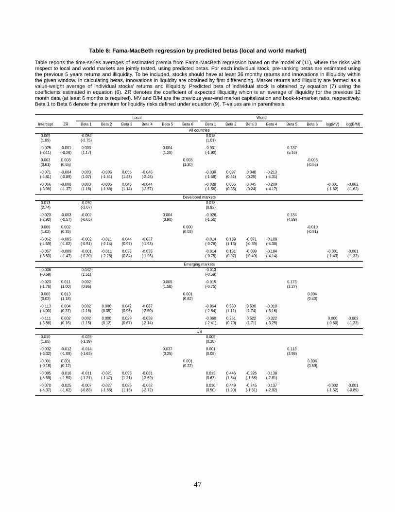
47

Table 6: Fama-MacBeth regression by predicted betas (local and world market) Table reports the time-series averages of estimated premia from Fama-MacBeth regression based on the model of (11), where the risks with respect to local and world markets are jointly tested, using predicted betas. For each individual stock, pre-ranking betas are estimated using the previous 5 years returns and illiquidity. To be included, stocks should have at least 36 monthy returns and innovations in illiquidity within the given window. In calculating betas, innovations in liquidity are obtained by first differencing. Market returns and illiquidity are formed as a value-weight average of individual stocks' returns and illiquidity. Predicted beta of individual stock is obtained by equation (7) using the coefficients estimated in equation (6). ZR denotes the coefficient of expected illiquidity which is an average of illiquidity for the previous 12 month data (at least 6 months is required). MV and B/M are the previous year-end market capitalization and book-to-market ratio, respectively. Beta 1 to Beta 6 denote the premium for liquidity risks defined under equation (9). T-values are in parenthesis.

Intercept ZR Beta 1 Beta 2 Beta 3 Beta 4 Beta 5 Beta 6 Beta 1 Beta 2 Beta 3 Beta 4 Beta 5 Beta 6 log(MV) log(B/M)

0.009 -0.054 0.018(1.89) (-2.75) (1.01)

-0.025 -0.001 0.003 0.004 -0.031 0.137(-3.11) (-0.28) (1.17) (1.28) (-1.90) (5.16)

0.003 0.003 0.003 -0.006(0.61) (0.65) (1.30) (-0.56)

-0.071 -0.004 0.003 -0.006 0.056 -0.046 -0.030 0.097 0.048 -0.213(-4.81) (-0.89) (1.07) (-1.61) (1.43) (-2.48) (-1.68) (0.61) (0.25) (-4.31)

-0.066 -0.008 0.003 -0.006 0.045 -0.044 -0.028 0.056 0.045 -0.209 -0.001 -0.002(-3.98) (-1.37) (1.16) (-1.68) (1.14) (-2.57) (-1.56) (0.35) (0.24) (-4.17) (-1.62) (-1.62)

0.013 -0.070 0.018(2.74) (-3.07) (0.92)

-0.023 -0.003 -0.002 0.004 -0.026 0.134(-2.93) (-0.57) (-0.65) (0.90) (-1.50) (4.89)

0.006 0.002 0.000 -0.010(1.02) (0.35) (0.03) (-0.91)

-0.062 -0.005 -0.002 -0.011 0.044 -0.037 -0.014 0.159 -0.071 -0.189(-4.69) (-1.02) (-0.51) (-2.14) (0.97) (-1.93) (-0.78) (1.13) (-0.39) (-4.30)

-0.057 -0.009 -0.001 -0.011 0.038 -0.035 -0.014 0.131 -0.089 -0.184 -0.001 -0.001(-3.53) (-1.47) (-0.20) (-2.25) (0.84) (-1.96) (-0.75) (0.97) (-0.49) (-4.14) (-1.43) (-1.33)

-0.006 0.042 -0.013(-0.69) (1.51) (-0.59)

-0.023 0.011 0.002 0.005 -0.015 0.173(-1.76) (1.00) (0.96) (1.58) (-0.75) (3.27)

0.000 0.013 0.001 0.006(0.02) (1.18) (0.62) (0.40)

-0.113 0.004 0.002 0.000 0.042 -0.067 -0.064 0.360 0.530 -0.318(-4.00) (0.37) (1.16) (0.05) (0.96) (-2.50) (-2.54) (1.11) (1.74) (-3.16)

-0.111 0.002 0.002 0.000 0.029 -0.058 -0.060 0.251 0.522 -0.322 0.000 -0.003(-3.86) (0.16) (1.15) (0.12) (0.67) (-2.14) (-2.41) (0.79) (1.71) (-3.25) (-0.50) (-1.23)

0.010 -0.028 0.005(1.85) (-1.39) (0.28)

-0.032 -0.012 -0.014 0.037 0.001 0.118(-3.32) (-1.09) (-1.63) (3.25) (0.08) (3.98)

-0.001 0.001 0.001 0.006(-0.18) (0.12) (0.22) (0.69)

-0.085 -0.016 -0.011 -0.021 0.096 -0.061 0.013 0.446 -0.326 -0.138(-6.69) (-1.50) (-1.21) (-1.42) (1.21) (-2.60) (0.67) (1.84) (-1.68) (-2.81)

-0.070 -0.025 -0.007 -0.027 0.085 -0.062 0.010 0.449 -0.245 -0.137 -0.002 -0.001(-4.37) (-1.62) (-0.83) (-1.86) (1.15) (-2.72) (0.50) (1.90) (-1.31) (-2.92) (-1.52) (-0.89)

Emerging markets

US

Local World

All countries

Developed markets

48

Table 7: Fama-MacBeth regression by predicted betas with respect to US market and Non-US world markets

Table reports the time-series averages of estimated premia from Fama-MacBeth regression based on the model specified in (12) derived from mildly-segmented world market model of (9), using predicted betas with respect to US market and Non-US world markets for the period of 1994-2004. Test assets do not include stocks from the US market. For each individual stock, pre-ranking betas are estimated using the previous 5 years returns and illiquidity. To be included, stocks should have at least 36 monthy returns and innovations in illiquidity within the given window. In calculating betas, innovations in liquidity are obtained by first differencing. Market returns and illiquidity are formed as a value-weight average of individual stocks' returns and illiquidity. Predicted beta of individual stock is obtained by equation (7) using the coefficients estimated in equation (6). ZR denotes the coefficient of expected illiquidity which is an average of illiquidity for the previous 12 month data (at least 6 months is required). MV and B/M are the previous year-end market capitalization and book-to-market ratio, respectively. Beta 1 to Beta 6 denote the premium for liquidity risks defined under equation (12). T-values are in parenthesis.

Intercept ZR Beta 1 Beta 2 Beta 3 Beta 4 Beta 5 Beta 1 Beta 2 Beta 3 Beta 4 Beta 5 log(MV) log(B/M)

-0.003 0.007 -0.030 -0.041(-0.38) (1.46) (-1.80) (-1.62)

-0.033 0.006 -0.019 -0.058 -0.048 0.243(-3.38) (1.23) (-0.90) (-0.47) (-1.88) (1.81)

-0.029 0.007 -0.048 -0.065 0.044 0.084(-2.47) (1.64) (-2.09) (-0.27) (1.25) (0.47)

-0.057 0.005 -0.010 -0.094 -0.036 -0.012(-3.16) (1.04) (-0.42) (-2.05) (-1.14) (-0.17)

-0.040 0.006 -0.010 0.045 -0.042 0.049(-3.75) (1.38) (-0.42) (1.34) (-1.48) (1.45)

-0.075 0.003 -0.026 -0.206 -0.051 -0.082 0.003 0.130 0.244 -0.008(-4.46) (0.71) (-1.01) (-0.96) (-0.20) (-1.41) (0.10) (1.27) (1.20) (-0.18)

-0.086 0.004 -0.029 -0.229 -0.123 -0.076 0.014 0.161 0.263 -0.010 0.000 0.000(-4.89) (0.73) (-1.09) (-1.08) (-0.48) (-1.34) (0.41) (1.46) (1.31) (-0.22) (0.61) (-0.43)

-0.003 0.006 -0.023 -0.060(-0.44) (1.29) (-1.35) (-2.37)

-0.025 0.005 -0.011 0.050 -0.066 0.117(-2.60) (1.01) (-0.55) (0.37) (-2.53) (0.99)

-0.030 0.005 -0.036 -0.098 0.051 0.095(-2.47) (1.12) (-1.59) (-0.40) (1.56) (0.48)

-0.038 0.005 -0.002 -0.117 -0.066 -0.003(-3.11) (1.02) (-0.10) (-2.31) (-2.16) (-0.09)

-0.028 0.005 -0.002 0.065 -0.061 0.016(-2.80) (1.15) (-0.11) (2.02) (-2.13) (0.49)

-0.053 0.002 -0.022 -0.092 -0.056 -0.090 0.012 0.098 0.185 -0.003(-3.71) (0.48) (-0.88) (-0.36) (-0.22) (-1.69) (0.36) (1.02) (0.92) (-0.06)

-0.064 0.003 -0.023 -0.109 -0.117 -0.079 0.019 0.134 0.207 -0.009 0.000 0.000(-4.11) (0.55) (-0.95) (-0.42) (-0.45) (-1.51) (0.61) (1.25) (1.04) (-0.21) (0.70) (-0.12)

-0.003 0.011 -0.019 0.027(-0.25) (0.97) (-0.59) (0.68)

-0.046 0.009 -0.037 -0.086 0.012 0.433(-2.30) (0.77) (-1.00) (-0.38) (0.26) (1.64)

-0.043 0.013 -0.064 -0.320 0.022 0.134(-2.47) (1.19) (-1.71) (-0.80) (0.37) (0.57)

-0.097 0.006 -0.031 -0.180 0.062 -0.054(-2.75) (0.46) (-0.72) (-2.13) (1.06) (-0.36)

-0.072 0.008 -0.025 0.106 0.037 0.132(-3.76) (0.73) (-0.60) (1.48) (0.68) (2.20)

-0.128 0.004 -0.045 0.087 -0.216 -0.153 -0.006 0.223 0.332 -0.076(-3.63) (0.38) (-1.12) (0.22) (-0.50) (-1.45) (-0.08) (1.24) (1.20) (-0.71)

-0.137 0.004 -0.054 0.038 -0.321 -0.156 0.007 0.253 0.319 -0.072 0.000 -0.002(-3.79) (0.34) (-1.40) (0.09) (-0.74) (-1.44) (0.09) (1.35) (1.18) (-0.63) (0.24) (-1.03)

Emerging markets

US Non-US

All countries (except US)

Developed markets (except US)

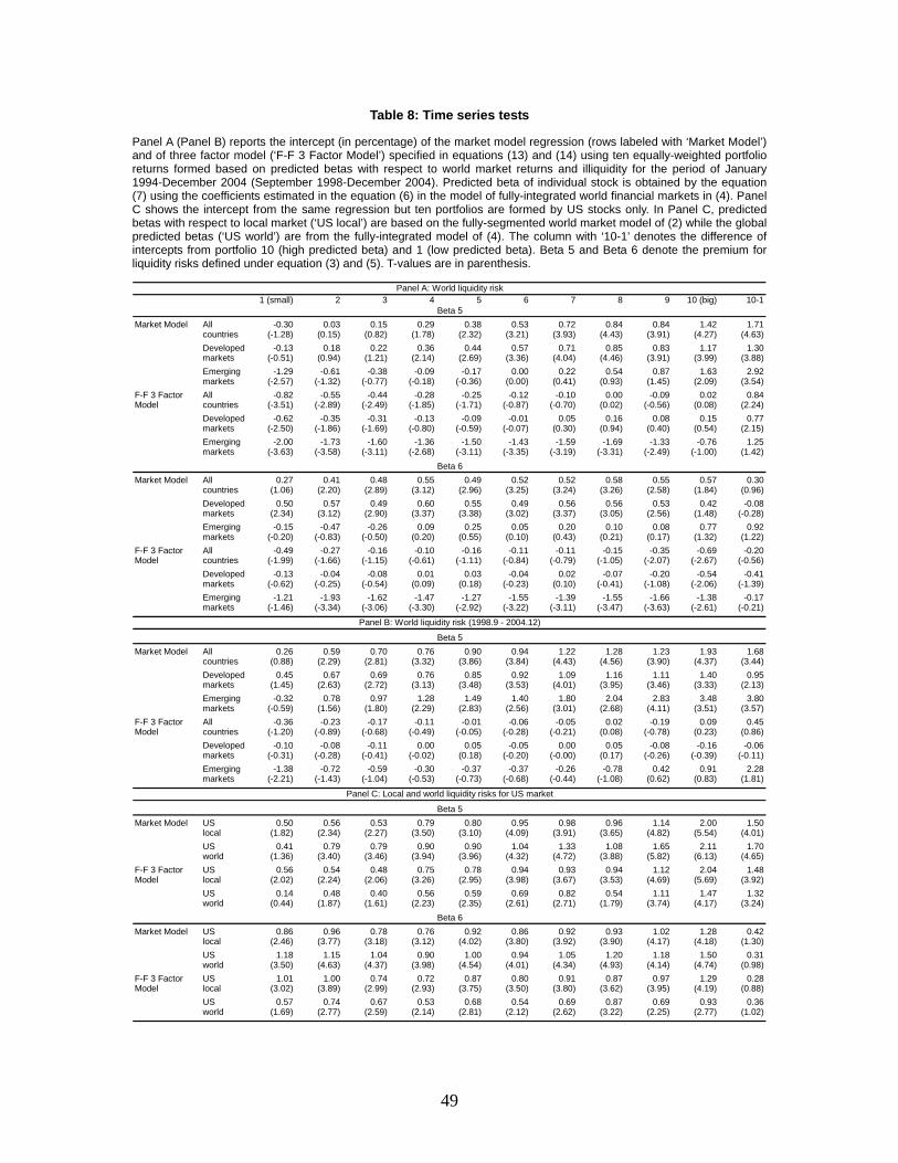
49

Table 8: Time series tests

Panel A (Panel B) reports the intercept (in percentage) of the market model regression (rows labeled with ‘Market Model’) and of three factor model (‘F-F 3 Factor Model’) specified in equations (13) and (14) using ten equally-weighted portfolio returns formed based on predicted betas with respect to world market returns and illiquidity for the period of January 1994-December 2004 (September 1998-December 2004). Predicted beta of individual stock is obtained by the equation (7) using the coefficients estimated in the equation (6) in the model of fully-integrated world financial markets in (4). Panel C shows the intercept from the same regression but ten portfolios are formed by US stocks only. In Panel C, predicted betas with respect to local market (‘US local’) are based on the fully-segmented world market model of (2) while the global predicted betas (‘US world’) are from the fully-integrated model of (4). The column with ‘10-1’ denotes the difference of intercepts from portfolio 10 (high predicted beta) and 1 (low predicted beta). Beta 5 and Beta 6 denote the premium for liquidity risks defined under equation (3) and (5). T-values are in parenthesis.

1 (small) 2 3 4 5 6 7 8 9 10 (big) 10-1

Market Model All -0.30 0.03 0.15 0.29 0.38 0.53 0.72 0.84 0.84 1.42 1.71countries (-1.28) (0.15) (0.82) (1.78) (2.32) (3.21) (3.93) (4.43) (3.91) (4.27) (4.63)Developed -0.13 0.18 0.22 0.36 0.44 0.57 0.71 0.85 0.83 1.17 1.30markets (-0.51) (0.94) (1.21) (2.14) (2.69) (3.36) (4.04) (4.46) (3.91) (3.99) (3.88)Emerging -1.29 -0.61 -0.38 -0.09 -0.17 0.00 0.22 0.54 0.87 1.63 2.92markets (-2.57) (-1.32) (-0.77) (-0.18) (-0.36) (0.00) (0.41) (0.93) (1.45) (2.09) (3.54)

F-F 3 Factor All -0.82 -0.55 -0.44 -0.28 -0.25 -0.12 -0.10 0.00 -0.09 0.02 0.84Model countries (-3.51) (-2.89) (-2.49) (-1.85) (-1.71) (-0.87) (-0.70) (0.02) (-0.56) (0.08) (2.24)

Developed -0.62 -0.35 -0.31 -0.13 -0.09 -0.01 0.05 0.16 0.08 0.15 0.77markets (-2.50) (-1.86) (-1.69) (-0.80) (-0.59) (-0.07) (0.30) (0.94) (0.40) (0.54) (2.15)Emerging -2.00 -1.73 -1.60 -1.36 -1.50 -1.43 -1.59 -1.69 -1.33 -0.76 1.25markets (-3.63) (-3.58) (-3.11) (-2.68) (-3.11) (-3.35) (-3.19) (-3.31) (-2.49) (-1.00) (1.42)

Market Model All 0.27 0.41 0.48 0.55 0.49 0.52 0.52 0.58 0.55 0.57 0.30countries (1.06) (2.20) (2.89) (3.12) (2.96) (3.25) (3.24) (3.26) (2.58) (1.84) (0.96)Developed 0.50 0.57 0.49 0.60 0.55 0.49 0.56 0.56 0.53 0.42 -0.08markets (2.34) (3.12) (2.90) (3.37) (3.38) (3.02) (3.37) (3.05) (2.56) (1.48) (-0.28)Emerging -0.15 -0.47 -0.26 0.09 0.25 0.05 0.20 0.10 0.08 0.77 0.92markets (-0.20) (-0.83) (-0.50) (0.20) (0.55) (0.10) (0.43) (0.21) (0.17) (1.32) (1.22)

F-F 3 Factor All -0.49 -0.27 -0.16 -0.10 -0.16 -0.11 -0.11 -0.15 -0.35 -0.69 -0.20Model countries (-1.99) (-1.66) (-1.15) (-0.61) (-1.11) (-0.84) (-0.79) (-1.05) (-2.07) (-2.67) (-0.56)

Developed -0.13 -0.04 -0.08 0.01 0.03 -0.04 0.02 -0.07 -0.20 -0.54 -0.41markets (-0.62) (-0.25) (-0.54) (0.09) (0.18) (-0.23) (0.10) (-0.41) (-1.08) (-2.06) (-1.39)Emerging -1.21 -1.93 -1.62 -1.47 -1.27 -1.55 -1.39 -1.55 -1.66 -1.38 -0.17markets (-1.46) (-3.34) (-3.06) (-3.30) (-2.92) (-3.22) (-3.11) (-3.47) (-3.63) (-2.61) (-0.21)

Market Model All 0.26 0.59 0.70 0.76 0.90 0.94 1.22 1.28 1.23 1.93 1.68countries (0.88) (2.29) (2.81) (3.32) (3.86) (3.84) (4.43) (4.56) (3.90) (4.37) (3.44)Developed 0.45 0.67 0.69 0.76 0.85 0.92 1.09 1.16 1.11 1.40 0.95markets (1.45) (2.63) (2.72) (3.13) (3.48) (3.53) (4.01) (3.95) (3.46) (3.33) (2.13)Emerging -0.32 0.78 0.97 1.28 1.49 1.40 1.80 2.04 2.83 3.48 3.80markets (-0.59) (1.56) (1.80) (2.29) (2.83) (2.56) (3.01) (2.68) (4.11) (3.51) (3.57)

F-F 3 Factor All -0.36 -0.23 -0.17 -0.11 -0.01 -0.06 -0.05 0.02 -0.19 0.09 0.45Model countries (-1.20) (-0.89) (-0.68) (-0.49) (-0.05) (-0.28) (-0.21) (0.08) (-0.78) (0.23) (0.86)

Developed -0.10 -0.08 -0.11 0.00 0.05 -0.05 0.00 0.05 -0.08 -0.16 -0.06markets (-0.31) (-0.28) (-0.41) (-0.02) (0.18) (-0.20) (-0.00) (0.17) (-0.26) (-0.39) (-0.11)Emerging -1.38 -0.72 -0.59 -0.30 -0.37 -0.37 -0.26 -0.78 0.42 0.91 2.28markets (-2.21) (-1.43) (-1.04) (-0.53) (-0.73) (-0.68) (-0.44) (-1.08) (0.62) (0.83) (1.81)

Market Model US 0.50 0.56 0.53 0.79 0.80 0.95 0.98 0.96 1.14 2.00 1.50local (1.82) (2.34) (2.27) (3.50) (3.10) (4.09) (3.91) (3.65) (4.82) (5.54) (4.01)US 0.41 0.79 0.79 0.90 0.90 1.04 1.33 1.08 1.65 2.11 1.70world (1.36) (3.40) (3.46) (3.94) (3.96) (4.32) (4.72) (3.88) (5.82) (6.13) (4.65)

F-F 3 Factor US 0.56 0.54 0.48 0.75 0.78 0.94 0.93 0.94 1.12 2.04 1.48Model local (2.02) (2.24) (2.06) (3.26) (2.95) (3.98) (3.67) (3.53) (4.69) (5.69) (3.92)

US 0.14 0.48 0.40 0.56 0.59 0.69 0.82 0.54 1.11 1.47 1.32world (0.44) (1.87) (1.61) (2.23) (2.35) (2.61) (2.71) (1.79) (3.74) (4.17) (3.24)

Market Model US 0.86 0.96 0.78 0.76 0.92 0.86 0.92 0.93 1.02 1.28 0.42local (2.46) (3.77) (3.18) (3.12) (4.02) (3.80) (3.92) (3.90) (4.17) (4.18) (1.30)US 1.18 1.15 1.04 0.90 1.00 0.94 1.05 1.20 1.18 1.50 0.31world (3.50) (4.63) (4.37) (3.98) (4.54) (4.01) (4.34) (4.93) (4.14) (4.74) (0.98)

F-F 3 Factor US 1.01 1.00 0.74 0.72 0.87 0.80 0.91 0.87 0.97 1.29 0.28Model local (3.02) (3.89) (2.99) (2.93) (3.75) (3.50) (3.80) (3.62) (3.95) (4.19) (0.88)

US 0.57 0.74 0.67 0.53 0.68 0.54 0.69 0.87 0.69 0.93 0.36world (1.69) (2.77) (2.59) (2.14) (2.81) (2.12) (2.62) (3.22) (2.25) (2.77) (1.02)

Panel A: World liquidity risk

Beta 5

Beta 5

Beta 6

Beta 6

Panel B: World liquidity risk (1998.9 - 2004.12)

Beta 5

Panel C: Local and world liquidity risks for US market

50

Table 9: Fama-MacBeth regression by global predicted betas (subperiod)

Table reports the time-series averages of estimated premia from Fama-MacBeth regression based on the fully-integrated world market model in (4) using predicted betas with respect to world market factors for two separate periods of January 1994 to August 1998 (panel A) and Septermber 1998 to December 2004 (panel B). For each individual stock, pre-ranking betas are estimated using the previous 5 years returns and illiquidity. To be included, stocks should have at least 36 monthy returns and innovations in illiquidity within the given window. In calculating betas, innovations in liquidity are obtained by first differencing. Market returns and illiquidity are formed as a value-weight average of individual stocks' returns and illiquidity. Predicted beta of individual stock is obtained by equation (7) using the coefficients estimated in equation (6). ZR denotes the coefficient of expected illiquidity which is an average of illiquidity for the previous 12 month data (at least 6 months is required). MV and B/M are the previous year-end market capitalization and book-to-market ratio, respectively. Beta 1 to Beta 6 denote the premium for liquidity risks defined under equation (4) and (5). T-values are in parenthesis.

Intercept ZR Beta 1 Beta 2 Beta 3 Beta 4 Beta 5 Beta 6 log(MV) log(B/M) Intercept ZR Beta 1 Beta 2 Beta 3 Beta 4 Beta 5 Beta 6 log(MV) log(B/M)

-0.004 -0.029 0.016 -0.010(-0.58) (-1.67) (2.74) (-0.83)

-0.035 0.000 -0.005 0.166 -0.015 -0.001 -0.014 0.112(-3.19) (-0.06) (-0.18) (3.11) (-1.56) (-0.11) (-0.95) (3.50)

-0.010 0.005 0.013 0.007 0.005 0.001(-1.32) (0.65) (0.78) (1.07) (0.80) (0.16)

-0.043 -0.002 0.012 -0.471 -1.106 -0.068 -0.030 -0.003 -0.012 0.364 -0.152 -0.044(-1.71) (-0.28) (0.44) (-2.41) (-3.13) (-1.00) (-1.68) (-0.55) (-0.73) (1.88) (-1.17) (-1.25)

-0.036 -0.008 0.012 -0.464 -1.158 -0.071 -0.002 -0.004 -0.024 -0.007 -0.008 0.241 -0.038 -0.063 -0.001 0.000(-1.38) (-0.90) (0.41) (-2.15) (-3.33) (-1.09) (-2.10) (-2.75) (-1.14) (-0.93) (-0.49) (1.27) (-0.27) (-1.82) (-1.07) (0.33)

-0.002 -0.047 0.019 -0.014(-0.31) (-2.84) (2.99) (-1.11)

-0.027 0.000 -0.030 0.136 -0.007 -0.002 -0.014 0.073(-2.98) (0.07) (-1.45) (3.20) (-0.74) (-0.30) (-1.00) (2.63)

-0.004 0.006 -0.010 0.011 0.003 -0.004(-0.61) (0.76) (-0.68) (1.55) (0.49) (-0.49)

-0.029 -0.001 -0.005 -0.519 -1.171 -0.003 -0.024 -0.005 -0.011 0.359 -0.001 -0.021(-1.07) (-0.15) (-0.21) (-2.73) (-3.12) (-0.03) (-1.26) (-0.80) (-0.64) (1.95) (-0.01) (-0.63)

-0.023 -0.007 -0.005 -0.475 -1.241 -0.004 -0.002 -0.003 -0.019 -0.009 -0.007 0.237 0.100 -0.040 -0.001 0.001(-0.78) (-0.85) (-0.22) (-2.24) (-3.33) (-0.05) (-2.03) (-2.49) (-0.80) (-1.04) (-0.40) (1.35) (0.74) (-1.22) (-0.91) (0.55)

-0.016 -0.009 0.018 0.003(-1.35) (-0.33) (1.96) (0.15)

-0.043 0.011 -0.003 0.156 -0.023 0.006 -0.010 0.207(-2.21) (0.62) (-0.10) (1.86) (-1.28) (0.45) (-0.53) (3.70)

-0.024 0.017 0.008 0.006 0.009 0.016(-1.40) (0.91) (0.33) (0.43) (0.62) (1.21)

-0.129 0.013 -0.024 -0.344 -0.039 -0.406 -0.059 0.006 -0.013 0.758 -0.519 -0.131(-3.22) (0.68) (-0.76) (-0.77) (-0.08) (-3.30) (-2.38) (0.39) (-0.60) (1.92) (-2.04) (-1.88)

-0.114 0.007 -0.022 -0.558 -0.150 -0.371 -0.001 -0.002 -0.062 0.003 -0.010 0.680 -0.364 -0.159 0.000 -0.002(-3.07) (0.35) (-0.73) (-1.38) (-0.31) (-2.89) (-0.72) (-0.91) (-2.45) (0.19) (-0.43) (1.71) (-1.22) (-2.59) (-0.11) (-0.72)

0.000 -0.022 0.025 -0.011(-0.02) (-1.41) (3.15) (-0.55)

-0.015 0.016 -0.021 0.084 -0.013 -0.019 -0.022 0.158(-1.48) (1.08) (-1.04) (3.06) (-0.90) (-1.16) (-0.93) (5.23)

-0.006 0.023 0.003 0.006 -0.003 0.013(-0.68) (1.62) (0.27) (0.60) (-0.19) (1.36)

-0.077 0.009 -0.014 -0.221 -0.269 -0.141 -0.048 -0.027 -0.017 0.717 0.052 -0.085(-4.25) (0.65) (-0.59) (-1.38) (-1.20) (-2.75) (-2.45) (-1.65) (-0.75) (2.47) (0.28) (-2.31)

-0.072 -0.001 -0.012 -0.152 -0.236 -0.147 -0.001 0.000 -0.039 -0.042 -0.012 0.540 0.074 -0.093 -0.004 -0.001(-3.34) (-0.06) (-0.54) (-1.01) (-1.08) (-3.18) (-0.66) (0.26) (-1.85) (-1.71) (-0.63) (2.08) (0.44) (-2.45) (-1.63) (-0.70)

Deveoploed markets

Emerging markets

US

Panel A: 1994.1 - 1998.8 Panel B: 1998.9 - 2004.12

All countries

51

Appendix 1: Fama-MacBeth regression with 25 portfolios for US market Table shows the time-series averages of estimated premia for illiquidity, market beta and liquidity betas for US market. Each 25 portfolio is formed based on the average illiquidity of the previous year (ZR portfolio), market capitalization (MV portfolio) and book-to-market ratio (B/M portfolio) at the end of previous year, respectively. Portfolio returns and illiquidity are obtained as equally-weighted averages of returns and illiquidity of member stocks, respectively. These portfolios are re-balanced every year. Each beta is estimated using the previous 5 years’ portfolio returns and illiquidity and the value-weighted US market return and illiquidity. The five-year window starts from January 1983 and is rolled forward at yearly intervals. Innovations in returns and illiquidity are obtained from AR(2) fitting using the entire time-series for 1983-2004 of each variable. Using estimated betas and illiquidity, cross-sectional regression is performed and the time-series averages of each coefficient are reported in the table. ZR denotes the coefficient of expected illiquidity which is an average of illiquidity for the previous 5 years data (at least 36 months is required). Beta 1-Beta 4 denote betas defined under equation (2). MV and B/M are a log of market capitalization and a log of book-to-market ratio, respectively, at the end of previous year. T-values are in parenthesis.

Intercept ZR Beta 1 Beta 2 Beta 3 Beta 4 log(MV) log(B/M)

B/M portfolio -0.025 0.478 0.019(-2.46) (4.23) (1.83)

-0.025 0.479 0.019 -0.178(-2.46) (4.26) (1.83) (-0.20)

-0.021 0.438 0.020 -0.299(-2.17) (3.87) (2.19) (-1.45)

-0.022 0.442 0.019 -0.070(-2.18) (3.94) (1.77) (-1.93)

-0.020 0.427 0.020 0.731 -0.111 -0.067(-2.13) (3.83) (2.19) (0.77) (-0.50) (-1.75)

0.006 0.269 0.017 -0.208 0.037 -0.027 -0.003 -0.001(0.60) (2.21) (2.41) (-0.24) (0.22) (-0.67) (-3.43) (-0.62)

ZR portfolio 0.031 -0.051 -0.018(3.84) (-1.42) (-2.14)

0.029 -0.040 -0.017 -0.052(3.70) (-1.01) (-2.11) (-0.04)

0.027 -0.052 -0.010 -0.701(3.31) (-1.43) (-1.25) (-3.30)

0.029 -0.032 -0.017 -0.010(3.75) (-0.97) (-2.01) (-0.25)

0.023 -0.019 -0.009 0.210 -0.702 -0.008(3.02) (-0.50) (-1.16) (0.15) (-3.39) (-0.19)

0.023 -0.052 -0.008 -0.253 -0.262 0.022 0.000 0.009(2.47) (-1.27) (-1.06) (-0.21) (-1.36) (0.52) (0.51) (2.81)

MV portfolio 0.004 0.209 -0.006(0.57) (2.88) (-0.63)

0.005 0.209 -0.005 -0.184(0.57) (2.68) (-0.52) (-0.10)

0.002 0.206 -0.001 -0.006(0.24) (2.83) (-0.14) (-0.03)

0.006 0.201 -0.008 0.028(0.82) (2.75) (-0.86) (0.78)

0.006 0.181 -0.004 -0.461 -0.025 0.035(0.79) (2.37) (-0.44) (-0.27) (-0.12) (1.04)

0.000 0.150 -0.002 -2.605 -0.039 0.078 0.001 0.002(0.01) (2.11) (-0.36) (-2.30) (-0.21) (2.33) (0.99) (0.73)

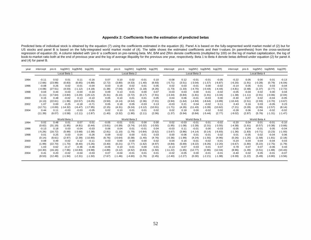
52

Appendix 2: Coefficients from the estimation of predicted betas Predicted beta of individual stock is obtained by the equation (7) using the coefficients estimated in the equation (6). Panel A is based on the fully-segmented world market model of (2) but for US stocks and panel B is based on the fully-integrated world market model of (4). The table shows the estimated coefficients and their t-values (in parenthesis) from the cross-sectional regression of equation (6). A column labeled with ‘pre-b’ a coefficient on pre-ranking beta. MV, B/M and ZRm denote coefficients (multiplied by 100) on the log of market capitalization, the log of book-to-market ratio both at the end of previous year and the log of average illiquidity for the previous one year, respectively. Beta 1 to Beta 4 denote betas defined under equation (2) for panel A and (4) for panel B.

year intercept pre-b log(MV) log(B/M) log(ZR) intercept pre-b log(MV) log(B/M) log(ZR) intercept pre-b log(MV) log(B/M) log(ZR) intercept pre-b log(MV) log(B/M) log(ZR)

1994 -0.11 0.52 0.01 0.11 -0.16 0.07 0.10 0.02 -0.01 0.10 -0.08 0.12 -0.01 -0.01 -0.05 -0.22 0.05 0.00 0.01 -0.13(-2.66) (23.98) (0.83) (6.65) (-6.88) (2.72) (3.80) (4.53) (-1.40) (6.93) (-5.71) (3.51) (-3.04) (-1.57) (-6.87) (-6.20) (1.91) (-0.28) (0.79) (-6.04)

1996 -0.08 0.26 0.02 -0.01 -0.04 0.03 0.18 0.02 0.01 0.05 0.02 0.03 -0.01 0.00 -0.02 -0.14 0.05 0.01 0.03 -0.04(-4.08) (27.51) (4.03) (-1.12) (-4.18) (1.38) (7.04) (3.87) (1.18) (4.26) (1.73) (1.33) (-4.70) (-0.44) (-4.44) (-4.81) (2.48) (1.37) (2.77) (-2.72)

1998 0.04 0.44 -0.03 -0.04 -0.34 0.09 0.13 0.01 0.00 0.07 -0.03 0.03 0.00 0.01 -0.02 -0.05 -0.04 0.02 0.00 0.04(1.11) (17.64) (-3.84) (-3.20) (-20.12) (5.31) (5.10) (3.72) (0.17) (7.91) (-3.34) (0.84) (1.81) (1.91) (-3.34) (-1.38) (-1.11) (2.91) (-0.06) (2.04)

2000 0.15 0.48 -0.02 0.13 -0.10 0.05 0.10 0.01 0.01 0.05 0.04 0.06 -0.01 -0.03 0.00 -0.30 0.07 0.02 -0.04 -0.05(4.13) (22.61) (-1.96) (10.57) (-6.05) (3.50) (4.14) (4.54) (2.36) (7.01) (3.94) (1.64) (-4.94) (-8.64) (-0.89) (-10.44) (2.51) (2.93) (-3.70) (-3.67)

2002 1.07 0.00 -0.25 -0.18 -0.71 0.05 0.18 0.05 -0.03 0.13 -0.03 0.21 0.04 -0.02 0.11 0.43 0.16 0.03 -0.05 0.23(12.71) (-0.00) (-14.32) (-6.47) (-17.95) (2.15) (4.31) (9.24) (-3.12) (10.91) (-1.71) (4.26) (11.43) (-3.39) (13.62) (7.21) (3.28) (2.06) (-2.57) (8.14)

2004 0.44 0.11 -0.03 -0.03 -0.05 0.02 0.10 0.01 0.01 0.02 0.02 0.18 0.00 -0.02 0.02 -0.28 0.06 0.04 -0.02 -0.02(11.39) (6.07) (-3.58) (-2.11) (-2.87) (1.40) (3.32) (1.90) (2.11) (2.06) (1.37) (5.94) (0.84) (-5.44) (2.77) (-9.02) (2.87) (5.76) (-1.31) (-1.47)

1994 0.02 0.48 0.01 0.07 0.01 -0.05 -0.01 0.01 0.00 0.00 0.02 -0.03 -0.01 0.01 -0.02 -0.20 0.04 0.01 -0.01 -0.10(0.62) (31.19) (1.95) (4.81) (0.44) (-3.61) (-0.39) (3.74) (-0.32) (-0.50) (1.95) (-1.08) (-2.28) (2.31) (-3.55) (-4.38) (1.61) (0.57) (-0.38) (-3.66)

1996 -0.13 0.18 0.03 -0.04 -0.03 0.06 0.04 0.01 -0.01 0.04 -0.03 0.11 -0.01 0.00 -0.03 -0.05 0.04 -0.01 0.05 -0.04(-5.26) (16.72) (5.99) (-3.68) (-2.38) (2.81) (1.10) (1.79) (-0.84) (3.52) (-3.67) (3.86) (-4.14) (0.14) (-5.83) (-1.36) (1.83) (-0.71) (3.23) (-1.93)

1998 0.01 0.25 0.03 0.04 -0.26 0.09 -0.02 0.00 0.01 0.03 0.00 -0.06 0.01 -0.01 0.02 0.01 -0.05 0.02 -0.04 0.06(0.14) (6.61) (2.97) (2.39) (-10.80) (6.76) (-0.64) (0.38) (1.40) (4.76) (-0.36) (-1.99) (4.24) (-1.55) (4.96) (0.26) (-1.25) (1.58) (-1.81) (2.18)

2000 0.08 0.49 -0.02 0.12 -0.11 0.03 0.00 0.00 0.00 0.02 0.04 0.16 -0.01 -0.02 -0.01 -0.24 0.04 0.04 -0.04 0.03(1.99) (22.70) (-1.70) (8.40) (-5.26) (3.40) (0.21) (2.77) (1.62) (4.97) (4.84) (5.69) (-8.22) (-8.26) (-2.20) (-6.67) (1.80) (5.22) (-2.75) (1.79)

2002 1.03 0.62 -0.17 -0.36 -0.46 -0.06 0.10 0.01 0.00 0.01 -0.13 0.07 0.03 0.01 0.07 0.78 0.07 0.07 -0.06 0.43(10.30) (16.16) (-7.96) (-10.83) (-9.98) (-4.89) (3.12) (4.52) (0.63) (1.50) (-11.22) (1.65) (12.77) (2.86) (12.04) (8.96) (1.39) (3.51) (-1.88) (10.43)

2004 0.41 0.20 -0.02 -0.04 -0.03 0.07 -0.04 -0.01 0.01 0.01 -0.02 -0.05 0.00 -0.01 -0.01 -0.40 0.02 0.05 -0.01 -0.07(8.53) (12.48) (-1.94) (-2.31) (-1.50) (7.67) (-1.46) (-4.60) (1.76) (2.45) (-2.40) (-2.27) (0.30) (-2.21) (-1.98) (-9.39) (1.22) (5.49) (-0.80) (-3.56)

Local Beta 1 Local Beta 2 Local Beta 3 Local Beta 4

World Beta 1 World Beta 2 World Beta 3 World Beta 4

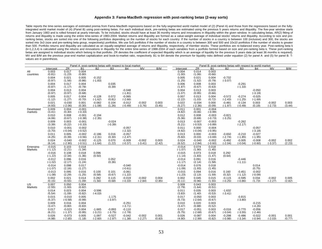
53

Appendix 3: Fama-MacBeth regression with post-ranking betas (2-way sorts)

Table reports the time-series averages of estimated premia from Fama-MacBeth regressions based on the fully-segmented world market model of (2) (Panel A) and those from the regressions based on the fully-integrated world market model of (4) (Panel B) using post-ranking betas. For each individual stock, pre-ranking betas are estimated using the previous 5 years returns and illiquidity. The five-year window starts from January 1983 and is rolled forward at yearly intervals. To be included, stocks should have at least 36 monthy returns and innovations in illiquidity within the given window. In calculating betas, AR(2) fitting of returns and illiquidity is made using the entire time-series of 1983-2004. Market returns and illiquidity are formed as a value-weight average of individual stocks' returns and illiquidity. According to size and pre-ranking betas, stocks are sorted into one of the following portfolios depending on the number of stocks for each country: If the number of stocks in a country is between 100 (inclusive) and 300, the stocks are sorted into 3x3 (size and pre-ranking beta group, respectively) portfolios. We use 5x5 portfolios if the number of stocks in a country is between 300 and 500 and 10x10 portfolios if the number of stocks is greater than 500. Portfolio returns and illiquidity are calculated as an equally-weighted average of returns and illiquidity, respectively, of member stocks. These portfolios are re-balanced every year. Post-ranking beta k (k=1,2,3,4) is calculated using the returns and innovations in illiquidity for the entire time-series of 1988-2004 of each variables from a portfolio formed based on size and pre-ranking beta k. These port-ranking betas are assigned to individual stocks which belong to that portfolio. ZR denotes the coefficient of expected illiquidity which is an average of liquidity for the previous 5 years data (at least 36 months is required). MV and B/M are the previous year-end market capitalization and book-to-market ratio, respectively. B1 to B4 denote the premium for liquidity risks defined under equation (2) for panel A and (5) for panel B. T-values are in parenthesis.

Panel A: post-ranking betas with respect to local market Panel B: post-ranking betas with respect to world market Intercept ZR B1 B2 B3 B4 MV B/M Intercept ZR B1 B2 B3 B4 MV B/M

All 0.003 0.017 0.004 0.004 0.014 0.003countries (0.81) (1.23) (0.80) (1.00) (1.06) (0.66) 0.004 0.021 0.005 -0.152 0.005 0.021 0.004 -0.732 (0.97) (1.56) (0.86) (-1.83) (1.25) (1.52) (0.79) (-3.07) 0.004 0.017 0.004 0.035 0.006 0.008 0.003 -0.291 (0.87) (1.17) (0.78) (0.39) (1.87) (0.67) (0.63) (-1.33) 0.004 0.013 0.004 -0.048 0.004 0.013 0.003 -0.050 (0.97) (0.97) (0.68) (-1.81) (1.07) (0.95) (0.66) (-3.19) 0.005 0.017 0.004 -0.128 0.072 -0.065 0.007 0.013 0.004 -0.572 -0.274 -0.025 (1.12) (1.27) (0.70) (-1.62) (0.81) (-2.66) (2.22) (1.03) (0.72) (-2.43) (-1.25) (-1.69) 0.021 -0.030 0.001 -0.082 0.104 -0.012 -0.002 0.003 0.022 -0.034 0.000 -0.481 -0.134 0.003 -0.002 0.003 (4.93) (-2.06) (0.30) (-1.08) (1.26) (-0.49) (-3.76) (3.45) (5.27) (-2.36) (0.09) (-1.97) (-0.49) (0.19) (-2.73) (3.44)Developed 0.009 0.004 -0.001 0.011 0.001 -0.004markets (3.41) (0.30) (-0.33) (4.82) (0.06) (-0.99) 0.010 0.008 -0.001 -0.194 0.012 0.008 -0.003 -0.821 (4.06) (0.67) (-0.38) (-2.35) (5.36) (0.69) (-0.73) (-3.25) 0.009 0.003 -0.001 -0.024 0.013 -0.007 -0.003 -0.262 (3.39) (0.22) (-0.33) (-0.39) (5.21) (-0.53) (-0.89) (-2.17) 0.010 -0.001 -0.002 -0.057 0.011 0.000 -0.004 -0.057 (3.70) (-0.04) (-0.52) (-2.32) (4.92) (-0.04) (-0.95) (-3.18) 0.011 0.005 -0.002 -0.186 0.016 -0.057 0.013 0.000 -0.003 -0.650 -0.210 -0.027 (4.25) (0.39) (-0.56) (-2.31) (0.30) (-2.47) (5.60) (0.03) (-0.69) (-2.74) (-1.85) (-1.95) 0.024 -0.040 -0.002 -0.125 0.070 -0.009 -0.002 0.003 0.024 -0.040 -0.002 -0.492 -0.005 -0.008 -0.002 0.002 (6.14) (-2.90) (-0.51) (-1.64) (1.22) (-0.37) (-3.41) (2.42) (6.52) (-2.84) (-0.60) (-2.04) (-0.04) (-0.60) (-3.37) (2.23)Emerging -0.015 0.103 0.018 -0.014 0.074 0.018Markets (-1.12) (2.21) (1.34) (-1.07) (1.90) (1.45) -0.016 0.108 0.018 0.096 -0.015 0.073 0.018 0.292 (-1.22) (2.34) (1.36) (0.50) (-1.14) (1.83) (1.47) (0.64) -0.012 0.096 0.016 0.052 -0.014 0.091 0.016 -0.446 (-1.02) (2.17) (1.24) (0.36) (-1.17) (2.14) (1.58) (-1.11) -0.014 0.098 0.017 -0.040 -0.014 0.076 0.018 0.014 (-1.07) (2.16) (1.27) (-0.61) (-1.09) (1.93) (1.45) (0.75) -0.013 0.095 0.016 0.100 0.101 -0.061 -0.015 0.094 0.016 0.160 -0.451 -0.002 (-1.08) (2.29) (1.25) (0.58) (0.67) (-1.22) (-1.23) (2.13) (1.59) (0.32) (-1.12) (-0.09) 0.002 0.021 0.014 0.282 0.115 -0.019 -0.002 0.004 0.002 0.045 0.015 -0.115 -0.595 0.034 -0.002 0.005 (0.15) (0.55) (1.09) (1.56) (0.68) (-0.33) (-2.84) (2.85) (0.11) (0.96) (1.55) (-0.25) (-0.86) (1.73) (-2.27) (2.82)US 0.007 0.050 0.004 0.009 0.043 0.003Markets (2.55) (1.93) (0.82) (2.79) (1.64) (0.51) 0.014 0.023 0.004 -3.596 0.011 0.035 0.003 -1.632 (5.54) (1.09) (0.82) (-4.03) (3.83) (1.40) (0.53) (-3.41) 0.015 -0.010 0.005 -1.175 0.017 -0.050 0.003 -0.815 (5.37) (-0.58) (0.99) (-3.97) (5.73) (-2.64) (0.67) (-3.80) 0.009 0.016 0.004 -0.251 0.010 0.020 0.003 -0.215 (3.47) (0.80) (0.83) (-3.71) (3.47) (0.88) (0.52) (-4.26) 0.017 -0.023 0.004 -1.665 -0.893 -0.110 0.017 -0.051 0.003 -0.016 -0.770 -0.056 (6.21) (-1.37) (0.95) (-3.21) (-3.75) (-2.78) (5.75) (-2.68) (0.67) (-0.04) (-3.55) (-2.46) 0.026 -0.073 0.005 -1.097 -0.527 -0.042 -0.002 0.001 0.026 -0.087 0.004 -0.298 -0.486 -0.022 -0.001 0.001 (4.98) (-2.65) (1.18) (-2.60) (-2.97) (-1.38) (-2.27) (0.83) (4.90) (-2.99) (0.82) (-0.98) (-3.34) (-0.94) (-2.03) (0.77)