the wind-driven overturning circulation of the world ocean

HAL Id: hal-00298451https://hal.archives-ouvertes.fr/hal-00298451

Submitted on 25 Nov 2005

HAL is a multi-disciplinary open accessarchive for the deposit and dissemination of sci-entific research documents, whether they are pub-lished or not. The documents may come fromteaching and research institutions in France orabroad, or from public or private research centers.

L’archive ouverte pluridisciplinaire HAL, estdestinée au dépôt et à la diffusion de documentsscientifiques de niveau recherche, publiés ou non,émanant des établissements d’enseignement et derecherche français ou étrangers, des laboratoirespublics ou privés.

The wind-driven overturning circulation of the WorldOceanK. Döös

To cite this version:K. Döös. The wind-driven overturning circulation of the World Ocean. Ocean Science Discussions,European Geosciences Union, 2005, 2 (5), pp.473-505. �hal-00298451�

https://hal.archives-ouvertes.fr/hal-00298451

https://hal.archives-ouvertes.fr

OSD2, 473–505, 2005

The wind-drivenoverturning

circulation of theWorld Ocean

K. Doos

Title Page

Abstract Introduction

Conclusions References

Tables Figures

J I

J I

Back Close

Full Screen / Esc

Print Version

Interactive Discussion

EGU

Ocean Science Discussions, 2, 473–505, 2005www.ocean-science.net/osd/2/473/SRef-ID: 1812-0822/osd/2005-2-473European Geosciences Union

Ocean ScienceDiscussions

Papers published in Ocean Science Discussions are underopen-access review for the journal Ocean Science

The wind-driven overturning circulationof the World OceanK. Doos

Department of Meteorology, Stockholm University, 10691 Stockholm, Sweden

Received: 18 October 2005 – Accepted: 25 October 2005 – Published: 25 November 2005

Correspondence to: K. Doos ([email protected])

© 2005 Author(s). This work is licensed under a Creative Commons License.

473

http://www.ocean-science.net/osd.htm

http://www.ocean-science.net/osd/2/473/osd-2-473_p.pdf

http://www.ocean-science.net/osd/2/473/comments.php

http://www.copernicus.org/EGU/EGU.html

OSD2, 473–505, 2005



K. Doos

Title Page



Tables Figures

J I

J I

Back Close

Full Screen / Esc

Print Version


EGU

Abstract

The wind driven aspects of the meridional overturning circulation of the world oceanand the Conveyor Belt is studied making use of a simple analytical model. The modelconsists of three reduced gravity layers with an inviscid Sverdrupian interior and awestern boundary layer. The net north-south exchange is made possible by setting5

appropriate western boundary conditions, so that most of the transport is confined tothe western boundary layer, while the interior is the Sverdrupian solution to the windstress. The flow across the equator is made possible by the change of potential vorticityby the Rayleigh friction in the western boundary layer, which is sufficient to permit waterand the Conveyor Belt to cross the equator. The cross-equatorial flow is driven by a10

weak meridional pressure gradient in opposite direction in the two layers on the equatorat the western boundary.

The model is applied to the World Ocean with a realistic wind stress. The amplitudeof the Conveyor Belt is set by the northward Ekman transport in the Southern Oceanand the outcropping latitude of the NADW. It is in this way possible to set the amount15

of NADW that is pumped up from the deep ocean and driven northward by the windand converted in the surface layer into less dense water by choosing the outcroppinglatitude and the depth of the layers at the western boundary. The model has proved tobe able to simulate many of the key features of the Conveyor Belt and the meridionaloverturning cells of the World Ocean. This despite that there is no deep ocan mixing20

and that the water mass conversions in the this model are made at the surface.

1. Introduction

The meridional overturning is the most important mechanism of the world ocean toexchange mass and heat between latitudes and ocean basins. The density differencebetween the cold and salty water of the North Atlantic and the fresher and warmer25

waters of the Pacific and the Indian Ocean is believed to drive the largest overturning

474





OSD2, 473–505, 2005



K. Doos

Title Page



Tables Figures

J I

J I

Back Close

Full Screen / Esc

Print Version


EGU

cell in the ocean, known as the Conveyor belt (Broecker, 1991). The North AtlanticDeep Water (NADW), which is formed by convection, constitutes the deeper part ofthe Conveyor Belt. The NADW travels south through the Atlantic into the SouthernOcean, where the NADW is ventilated or continues in the deep ocean into the Pacificor Indian Oceans. Once the water emerges at the surface it can return to the North5

Atlantic along the upper part of the Conveyor Belt. The return route has been a subjectfor discussion, whether the water comes mainly through the Drake Passage and thenflows north into the Atlantic along the “cold water route” (Rintoul, 1991) or goes fromthe Pacific through the Indonesian Sea into the Indian Ocean around South Africa andthen into the Atlantic in the “warm water route” (Gordon, 1986).10

The Conveyor Belt is thus the greatest inter-ocean exchange of mass and heat. TheConveyor Belt is often presented as a fundamentally non-linear phenomenon and isdriven by the high-latitude buoyancy flow to the atmosphere and by deep convection.Accordingly it has been mostly discussed diagnostically using numerical general cir-culation models (GCMs) (e.g. Drijfhout, 1996; Speich et al., 2002). Such discussions15

cannot examine the broader aspects of the physics involved because of the complex-ities (numerical and geographical) of the GCM solutions. However, it is possible toaddress many (but not all) aspects of the Conveyor Belt with simple, mostly analytical,models; this is the idea behind this article.

The purpose of this study is to explore to what extent the ocean overturning circu-20

lation and in particular the Conveyor Belt can be explained by the wind driven oceandynamics. This will be done by using an as simple wind driven model as possiblebut that still captures the basic overturning circulation as seen in General CirculationModels (GCMs). The key features of the Conveyor Belt which must be included are apole-ward surface, and an equator-ward subsurface flow. The simplest model, which25

would include these, is a layered model. We choose a three-and-a-half layered modelsimilar to that of Doos (1994) and Nof (2003). This choice automatically brings somedisadvantages, chief among which is the lack of thermodynamics. At first sight thismay seen a telling difficulty, since deep convection, one essential component of the

475





OSD2, 473–505, 2005



K. Doos

Title Page



Tables Figures

J I

J I

Back Close

Full Screen / Esc

Print Version


EGU

Conveyor Belt, is explicitly excluded in what is primarily a wind-driven model. Althoughthere are ad hoc methods for including thermodynamics in a layered model, these areunsatisfactory and remove the clarity sought in the first place. Accordingly, all areaswhere thermodynamics play a crucial role are placed logically and geographically be-yond the boundaries of the model. The amplitude of the Conveyor Belt must then be5

provided for the model.A description of the model is presented in Sect. 2. The model is applied to the World

Ocean together with a fine resolution primitive equation model in Sect. 3. The simula-tion of the wind driven cells with a particular focus on the Conveyor Belt is presentedin Sect. 4 followed by a discussion and conclusions in Sect. 5.10

2. The analytical model

The dynamics of the model are Sverdrupian in the interior with a Stommel layer atthe western boundary (Stommel, 1948). By including a western boundary layer it ispossible to calculate net meridional transports and the corresponding meridional over-turning stream function. Three reduced gravity layers are used, and an Ekman layer15

in the extra-equatorial regions. The physical model is shown in Figs. 1 and 2. Theequations of motion for the Ekman layer are:

−f vE = T x

ρ0hEf uE = T y

ρ0hE

wE = 1ρ0∇ ×

(TW

f

) (1)

The equations of motion and the continuity equation for layer 1 are:

−f v1 = −∂G1∂x

f u1 = −∂G1∂y − Γ v1

∂u1∂x + ∂v1

∂y + ∂w1∂z = 0

(2)

20

476





OSD2, 473–505, 2005



K. Doos

Title Page



Tables Figures

J I

J I

Back Close

Full Screen / Esc

Print Version


EGU

and for layer 2:

−f v2 = −∂G2∂x

f u2 = −∂G2∂y − Γ v2

∂u2∂x + ∂v2

∂y + ∂w2∂z = 0

(3)

and for layer 3:

−f v3 = −∂G3∂x

f u3 = −∂G3∂y − Γ v3

∂u3∂x + ∂v3

∂y + ∂w3∂z = 0

(4)

where for simplicity the coordinates are Cartesian here but all the calculations5

have been made with spherical coordinates. x is pointing eastward, y northward,f is the Coriolis parameter as a function of latitude, hn is the n-th layer’s thick-ness and G1≡γ1h1+G2, G2≡γ2 (h1+h2)+G3 and G3≡γ3 (h1+h2+h3). Γ is the bot-tom friction coefficient. Under the Boussinesq approximation a reference densitycan be used in the denominator for the reduced gravity in each active layer so that10

γn≡2g (ρn+1−ρn)/ (ρn+1+ρn) is the reduced gravity. T X and T Y are the zonal and

meridional wind stresses and TW(T X , T Y

)is the wind stress vector. Layer 4 is inert

due to our reduced-gravity assumption.The model is constructed in a similar way as Stommel (1948) solved the western

boundary current problem by separating the ocean in in a frictionless interior and a15

western boundary layer with linear friction.

2.1. Interior of the ocean

The dynamics are Sverdrupian in the interior of the ocean, i.e. under the Ekman layerand outside the western boundary layer, where the friction terms are small. The equa-tions can here be solved using the equations for the ventilated thermocline by Luten20

477





OSD2, 473–505, 2005



K. Doos

Title Page



Tables Figures

J I

J I

Back Close

Full Screen / Esc

Print Version


EGU

et al. (1983) (hereafter denoted LPS). These solutions are presented in the Appendix.The LPS theory has of course in its simplicity many limitations such as e.g. that all butone active layer must vanish on the eastern boundary. Moreover, the thickness of thatlayer defines the width of the “shadow zones” in the solution. From the depths of thelayer interfaces it is possible to calculate the meridional velocity fields geostrophically5

everywhere except at the equator.

2.2. Western boundary layer

The friction is only kept in the western boundary layer as a linear Rayleigh friction inthe meridional equation. The other friction terms have been neglected. The frictionin the zonal equation of momentum will otherwise only have a smoothing effect on10

the solutions. Note however, that in order to have a more realistic parameterisationof the the friction one can use e.g. Laplacian viscosity (Munk, 1950) in particular atthe Equator where it plays an essential role in the strong zonal Equatorial currents.This has been tested but does not alter the results and we have therefore chosen tokeep the model as simple as possible. In order to simulate the Equatorial currents one15

requires vertical advection and friction of momentum between the layers which is adegree of complexity above the present model, which would anyhow not contribute tothe meridional overturning circulation.

From (2)–(4) it is possible to derive equations for the layer thicknesses h1, h2 and h3:

Γ ∂∂x

(h1

∂G1∂x

)+ βh1

∂G1∂x = f J (G1, h1) − f 2wE

Γ ∂∂x

(h2

∂G2∂x

)+ βh2

∂G2∂x = f J (G2, h2)

Γ ∂∂x

(h3

∂G3∂x

)+ βh3

∂G3∂x = f J (G3, h3)

(5)

20

where β≡∂f /∂y and the Jacobian J (a, b)≡∂a∂x

∂b∂y−

∂a∂y

∂b∂x .

The layer thicknesses hn, can be solved with Eq. (5) at all latitudes. Different so-lutions will be found for the interior of the ocean, the western boundary layer and the

478





OSD2, 473–505, 2005



K. Doos

Title Page



Tables Figures

J I

J I

Back Close

Full Screen / Esc

Print Version


EGU

Equatorial region.In the western boundary layer the friction terms balances the planetary vorticity. A

second order ordinary differential Eq. (5) is obtained which cannot be solved analyti-cally in the western boundary region except for when only one layer is active (Stommel,1948). Thus, the solution in this region must be obtained numerically. These types of5

equations are often integrated in time but since these equations are time independentthey have to be solved with an iterative numerical solution of Eq. (5). The solutionconverges within a few iteration to a unique solution. The choice of friction determinesthe width of the western boundary layer. With a friction coefficient of Γ=1/(7 days), theStommel layer thickness (δ=Γ/β) is in the zonal direction 0.7◦ at the Equator and 2.6◦

10

at 60◦. The width of the western boundary region, where the iterative semi-analyticalsolution is applied, is set to 5◦, so that the boundary layer is well solved at all latitudes.This type of model is otherwise insensitive to the choice of friction coefficient and thesimulated overturning circulation does not alter.

The depths of the layer interfaces in Eq. (5) require three western boundary condi-15

tions, which are set by the total northward transport in each layer Vn=∫xExWvnhndx which

in turn is determined geostrophically from zonal momentum equations in Eqs. (2)–(4)by the depth at the western boundary so that

V1 =∫xExW

h1f∂G1∂x dx

V2 =∫xExW

h2f∂G2∂x dx

V3 =∫xExW

h3f∂G3∂x dx

(6)

where the indices W and E indicate respectively the western and eastern boundaries.20

Using these expressions it is possible to calculate numerically by simple iteration thedepths of the layers at the western boundary corresponding to a meridional transportVn for each layer.

479





OSD2, 473–505, 2005



K. Doos

Title Page



Tables Figures

J I

J I

Back Close

Full Screen / Esc

Print Version


EGU

The total meridional transport across a basin including the Ekman transport is:

V1 + V2 + V3 + Ve =γ32f

(D2E − D2

W

)+ γ2

2f

(H2E − H2

W

)−

γ12f h

21W − 1

f ρ0

∫xExWT xdx

(7)

where D is the depth of layer 3 and H is the depth of layer 2. The individual valuesof the meridional transport Vn that sets the three western boundary conditions will bediscussed in Sect. 4 for each ocean basin.5

2.3. Application of the model to the World Ocean

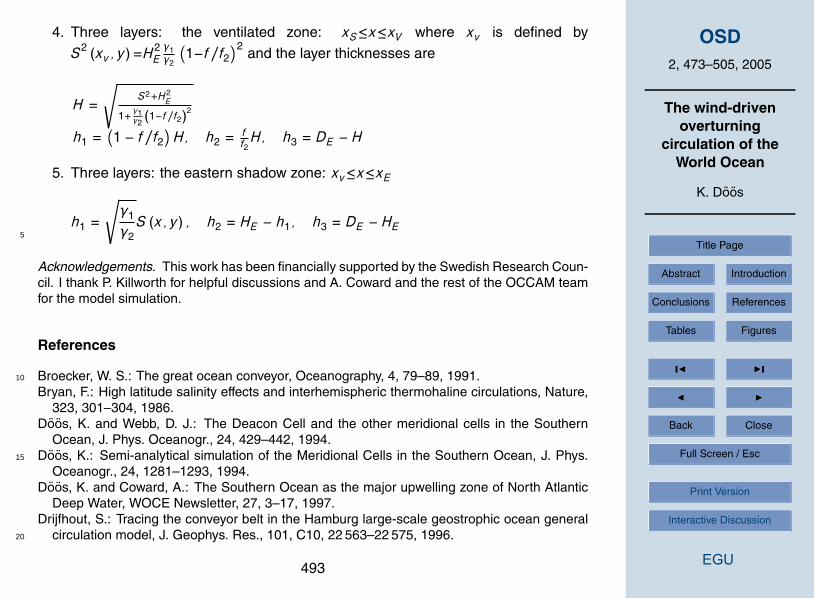
We now apply the model to the World Ocean. The aim is to see to what extent themodel can simulate the meridional overturning cells. The wind stress used is theyearly average of the ECMWF climatology analysis by Trenberth et al. (1989). TheLPS regions (see Appendix), which determine the dynamics of the interior solution,10

are presented in Fig. 3. LPS argued in their study that their particular choice of densitylayers were arbitrary. The choice is however here close to theirs: ρ1=1025.5 kg/m3,ρ2=1027.2 kg/m3, ρ3=1027.55 kg/m3 and ρ4=1028.2 kg/m3. The depths of the in-terfaces between layer 2, 3 and 4 at the eastern boundary have been chosen toHE=1400 m and DE=3200 m. The choice of these depths have been made to fit the15

depths of the deep branches of the meridional cells in OCCAM. Different values of thedepths will simply move the meridional circulation up or down. The deepest layer 3 isin the interior only active in the very southern Southern Ocean where layer 2 outcropsbecause of the strong Ekman upwelling. All layers with non zero depths are active inthe western boundary layer governed by Eq. (5). The depths of the interfaces between20

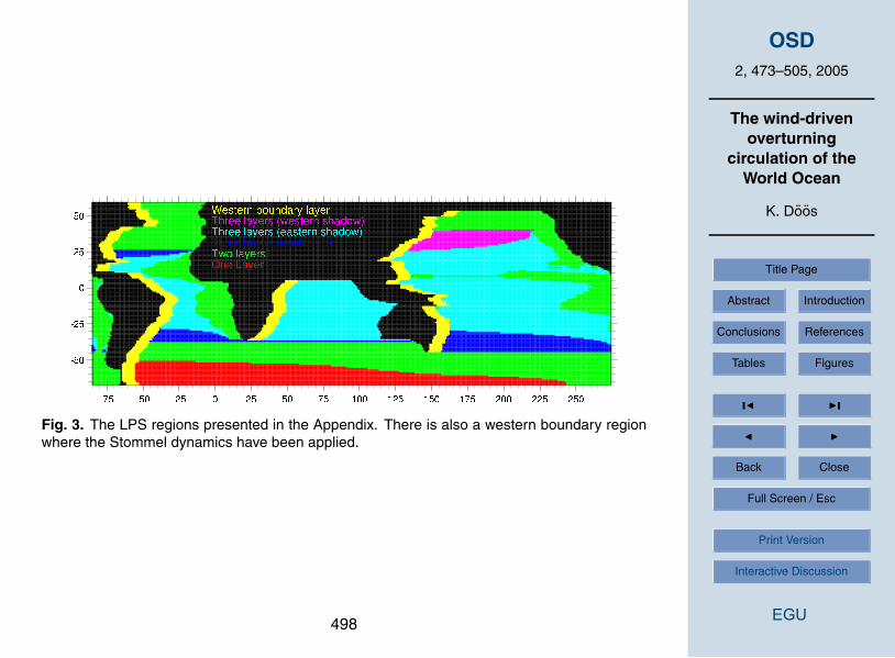
the layers are presented in Fig. 4.Since the model has no active thermodynamics it cannot simulate the positions of

the outcropping latitudes y2N and y2S . They are instead prescribed and are presentedin Table 1. These chosen latitudes are also shown in comparison with the sea surface

480





OSD2, 473–505, 2005



K. Doos

Title Page



Tables Figures

J I

J I

Back Close

Full Screen / Esc

Print Version


EGU

density in OCCAM in Fig. 5. The thermohaline forcing is also set by the outcroppinglatitude y3 in the Southern Ocean, which is set indirectly by the choice of the depth oflayer three at the eastern boundary (DE ).

2.4. Equatorial region

At the Equator, where the Ekman dynamics are not valid, we need to apply the wind5

stress directly to the shallowest reduced gravity layer. The depths of the layers for theinterior of the ocean can be solved from Eq. (5). The difference is, however, that thereis no meridional Ekman transport above the surface layer, implying that the meridionalvelocities cannot be calculated from the geostrophic velocities. Instead they have to beobtained by applying directly the wind stress on the shallowest reduced gravity layer.10

The deep layers, which are not in contact with the surface, are of constant interfacedepths along the equator. Only the interface depth between the surface layer and thelayer below will be affected by the wind stress. If layer 1 is non zero then the zonalequations of motions in Eqs. (1)–(4) are replaced by

0 = −γ3∂D∂x − γ2

∂H∂x − γ1

∂h1∂x + T x

ρ0h1

0 = −γ3∂D∂x − γ2

∂H∂x

0 = −γ3∂D∂x

(8)15

From which it is possible to derive expressions for the layer interfaces by integratingfrom the eastern boundary with the appropriate eastern boundary conditions:

h1(x) =√h2

1E − 2γ1ρ0

∫xEx T xdx′

H (x) = HED(x) = DE

(9)

481





OSD2, 473–505, 2005



K. Doos

Title Page



Tables Figures

J I

J I

Back Close

Full Screen / Esc

Print Version


EGU

Similarly if layer 2 is in contact with the atmosphere then

h1(x) = 0

H (x) =√H2E − 2

γ2ρ0

∫xEx T xdx′,

D(x) = DE

(10)

In the interior these equations are identical to the LPS solutions given in the Appendixfor the eastern shadow zone and the two layer solutions. In the western boundaryregion the matching is also without any discontinuity as seen in Fig. 6, which is a result5

of the meridional “mixing” arising from the Jacobian in Eq. (5).Away from the western boundary, it is the zonally static solution for the equatorial

region where the zonal pressure gradient is balanced by the zonal wind stress. Theequatorial currents are filtered out since there is no vertical advection, nor vertical dif-fusion of momentum in the zonal Eqs. (2)–(4). Apart from the Sverdrupian wind driven10

surface layer currents the cross Equatorial flow has to take place in the western bound-ary layer. This is possible if there is a meridional pressure gradient, the meridionalequations in Eqs. (2)–(4) become at the equator:

v1 = − 1Γ∂G1∂x

v2 = − 1Γ∂G2∂x

v3 = − 1Γ∂G3∂x

(11)

The depth of the layer interfaces at the western boundary (Fig. 6), which we cal-15

culated in the previous paragraph, have clear meridional gradients, which will enablethe water to cross the equator. Water flow across the equator is far from understood,since it requires a change in sign of the potential vorticity. In this analytical model theRayleigh friction is adequate to change this sign of the potential vorticity, but no claimsare made other than this is the simplest addition to the wind driven geostrophic dy-20

namics which permit inter-hemisphere transports. Since this friction is also necessaryto close the western boundary layer, there is no need to make use of more complex

482





OSD2, 473–505, 2005



K. Doos

Title Page



Tables Figures

J I

J I

Back Close

Full Screen / Esc

Print Version


EGU

dynamics. Note also that the depth of the layer interfaces at the western boundary inFig. 6, depends on the shape of the western boundary and the strength of the Sver-drup Circulation at the western boundary. This is why the meridional gradient of thedepths of the layer interfaces at the western boundary in the Atlantic changes sign ataround 40◦ N where, the Sverdrup circulation changes sign and the American coast5

line reaches its easternmost longitude. This is also where the biggest changes of thecoastline occurs, which explains the rather noisy behaviour of the depths of the layerinterfaces.

3. The Ocean general circulation model OCCAM

The aim is of the present study is to see to what extent our model model can simulate10

the meridional overturning cells. At the present date, only numerical models can pro-vide complete pictures of the world meridional circulation. However observational datado exist in some key areas of the world ocean but it is beyond the scope of this paperto validate the numerical models. We have here opted to use the general circulationmodel OCCAM to represent the “true” ocean circulation.15

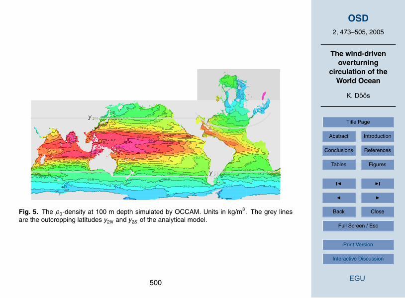
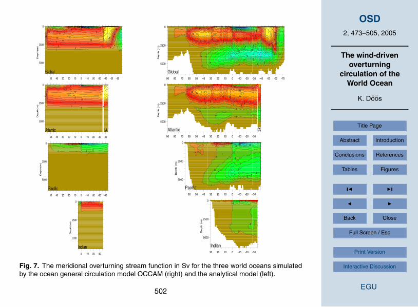
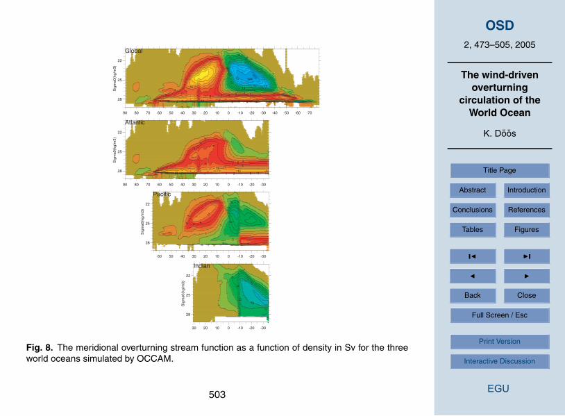
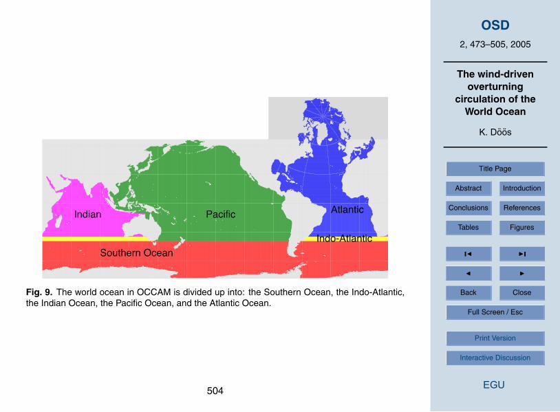
OCCAM has a horizontal 1/4◦ resolution at the equator with 66 depth levels. Theused model integration are taken from the years 1991 to 2002 (Marsh et al., 2005). Themeridional stream function from OCCAM is presented in Figs. 7 and 8 for the differentworld ocean basins defined in Fig. 9. The Atlantic, North Pacific and Southern Ocean

have nearly zero net meridional transport apart from 0.6 Sv(

1 Sv=106 m/s2)

through20

the Bering Strait. There is a net barotropic circulation of about 13 Sv around Australia,which flows through the Indonesian Sea. The meridional stream function is therefore byintegrating from the bottom and up to the surface, 13 Sv in the Pacific west of Australiaand −13 Sv in the Indian and the Indo-Atlantic east of Australia. The Indian and Pacifichave been split up in the middle of the Indonesian Sea. The stream function is hence25

gradually decreasing to zero at the surface between the north Australian continent and

483





OSD2, 473–505, 2005



K. Doos

Title Page



Tables Figures

J I

J I

Back Close

Full Screen / Esc

Print Version


EGU

the south Asian continent.The key feature of the meridional circulation is the Conveyor Belt, which is clearly

illustrated by the cell in the Atlantic with a maximum of 18 Sv at 30◦ S at about 1500 mdepth. This cell decreases towards the north, and in the very north corresponds tothe formation of the North Atlantic Deep Water (NADW). Further south it can unfortu-5

nately not correspond to any real formation of NADW since in this region the surfaceconditions are not such as can significantly contribute to the NADW south of 50◦ N, andthereby intensify the spin-up process in OCCAM.

4. The overturning circulation simulated by the analytical model

In order to understand the simulation of the ocean circulation and in particular its10

overturning component we will follow the path of the Conveyor Belt from the South-ern Ocean where the NADW upwells and around the cycle in the world ocean. Aschematic view of the model is presented in Fig. 2 with corresponding outcropping lat-itudes as well as density layer transports. The choices of outcropping latitudes in theanalytical model presented in Table 1 determine the water mass exchange between15

the density layers by the Ekman transport in the Ekman layers across these latitudes.

4.1. The Southern Ocean

The NADW upwells from the deep ocean (layer 3) into the Ekman layer at the surfaceof the Southern Ocean. It is the amplitude of the northward Ekman transport from layer3 into layer 2 across their interface at y3S (x) sets the amplitude of the Conveyor Belt:20

VCB = E (y3S (x))

where E is the zonally integrated Ekman transport across the line y3S (x) (see Fig. 2).Once the NADW is in the Ekman layer it changes water mass characteristics duringits flow northward into layer 2 across y3S (x). This is the driving force of the Conveyor

484





OSD2, 473–505, 2005



K. Doos

Title Page



Tables Figures

J I

J I

Back Close

Full Screen / Esc

Print Version


EGU

Belt in this analytical model. The strength of the conveyor belt (VCB) is in the analyt-ical model 16 Sv, which can be compared with the 18 Sv by the OCCAM integration.Most estimates are between 16 and 20 Sv by different numerical simulations (Semt-ner and Chervin, 1992; Stevens and Thompson, 1994). The inverse model basedon hydrographic data by Ganachaud and Wunch (2000) estimates the Conveyor Belt5

component in the South Atlantic to 16±3 Sv.The transport continues north in the Ekman layer and layer 2:

V2 (y) + E (y) = VCB f or y3 (x) ≤ y ≤ yAus

where V2 is the total transport of layer 2. At the latitude of south Australia(yAus=44◦ S

),

the northward flowing Conveyor Belt is split up into one branch that flows into the the10

Pacific and one into the Indo-Atlantic.There is also an Antarctic Bottom Water (AABW) Cell simulated by the analytical

model in the Southern ocean. There is however no northward penetration of the AABWcell in the world ocean as in the OCCAM integration. The AABW Cell is instead onlya one layer cell in the Southern Ocean. The reason for this is that we do not have15

any subsurface diapycnal mixing in our simple analytical model. The AABW is in OC-CAM mixing with less dense water such as the NADW. Although the AABW is loosingrelatively little buoyancy in OCCAM, which explains why the AABW Cell is very thin inthe stream function as a function of density in Fig. 8, it still corresponds to a verticaldisplacement of several thousands of meters in Fig. 7 since the ocean is only weekly20

stratified in the deep ocean.

4.2. The Pacific Ocean

The total transport into the Pacific is also the transport through the Indonesian Sea(VTF ) since we do not have any evaporation-precipitation and that Bering Strait isclosed. The amplitude of the Indonesian through flow is in our model set by how much25

water is converted from intermediate water of layer 2 into tropical water of layer 1. Thisis in turn forced by the equatorward Ekman transport across the outcropping latitudes

485





OSD2, 473–505, 2005



K. Doos

Title Page



Tables Figures

J I

J I

Back Close

Full Screen / Esc

Print Version


EGU

of y2Sand y2N between layer 1 and 2 in the Pacific so that the Indonesian through flowis

VTF = EP (y2S ) − EP (y2N )

Note that in our analytical model there is no deep water (NADW or AABW) flowing intothe Pacific, since all the NADW upwells in the Southern Ocean. At yInd the Conveyor5

Belt flows through Indonesian Sea and into the Indian. By using our chosen valuesof outcropping latitudes in Table 1 we obtain an Indonesian through flow transport ofVTF=9.3 Sv, which is lower than that of the 13 Sv of the OCCAM integration and theestimated 16±5 Sv by Ganachaud and Wunsh (2000).

4.3. The Indian10

The Indonesian through flow enters the Indian where it continues south together withthe return flow of the northward Ekman transport. The model fails to find a pure LPSsolution in the Indian basin that satisfies the boundary conditions without having anegative depth at the western boundary, which would have no physical meaning. Adepth of 450 m at the eastern boundary for layer 1 has therefore been applied instead15

of the usual h1E=0. This implies unfortunately an inconsistency with a discontinuity ofthe layer 1 thickness at the eastern boundary between the Indo-Atlantic and the Indian(xE , yAfr). Doos (1994) argued that the failure of the LPS theory in the Indian couldbe linked to the southward boundary current along the coast of Australia (LeeuwinCurrent).20

The Conveyor Belt can now continue its path along the African coast into the AghulasCurrent and then turns around at and enters the Atlantic Basin into layer 2.

4.4. The Indo-Atlantic

Let us now return to the latitude of South Australia (yAus), and follow the northwardtransport that enters the Indo-Atlantic from the Southern Ocean Basin in layer 2 and25

486





OSD2, 473–505, 2005



K. Doos

Title Page



Tables Figures

J I

J I

Back Close

Full Screen / Esc

Print Version


EGU

the Ekman layer where

V2 (y) + E (y) = VCB − VTF f or yAus ≤ y ≤ y2S

But since the northward Ekman transport is E (y)>VCB−VTF we must have V2 (y)<0,which becomes a southward return flow forming the Deacon Cell, which is the anti-clockwise cell in the Indo-Atlantic. The outcropping latitude y2S determines the strength5

of the Deacon Cell, since all the water that does not continue north in the Ekman layerat y2S must return south in layer 2. The depth of the Deacon Cell is deeper in OCCAMthan in our model. Doos (1994) demonstrated however that by having an easternboundary depth of layer 2 (HE ) of 2750 m instead of the present 1400 m it was possibleto simulate the Deacon Cell at the right depth.10

The transport in layer 2 north of y2S is

V2 (y) = VCB − E (y2N ) − VTF for y2S ≤ y ≤ yAfr

4.5. The Atlantic Basin

The two shallow branches of the Conveyor Belt, which are sometimes referred in theliterature to as the Warm and Cold Water Paths, merge at yAfr when they flow north15

into the Atlantic Basin. The transport through the surface layers is driven by the Ekmantransport at the outcropping latitude in the north Atlantic:

V1 (y) − E (y) = E (y2N ) for yAfr ≤ y ≤ y2N

The transport in layer 2 is hence by continuity:

V2 = VCB − E (y2N ) for yAfr ≤ y ≤ y2N20

The northward return flow is in this way divided into one shallow branch and one in-termediate branch. At the outcropping latitude in the North Atlantic the two branchesmerge in layer 2 and continue north to the convection area:

V2 (y) = VCB − E (y) for y2N ≤ y ≤ yC487





OSD2, 473–505, 2005



K. Doos

Title Page



Tables Figures

J I

J I

Back Close

Full Screen / Esc

Print Version


EGU

This model can of course not simulate the convection processes that enables theformation of NADW in layer three. The convection from layer 2 to layer 3 takes placebetween the latitudes yC and yN . This convection zone only prescribes the transportfrom layer two to layer three where the NADW starts its southward journey:

V2 = −V3 =yN − yyN − yC

VCB for yC ≤ y ≤ yN5

The NADW flows south in layer 3 without any exchange to other layers until it outcropsin the Southern Ocean at y3 (x), which brings us back to where we started to trace theConveyor Belt.

4.6. The tropical cells

The tropical shallow meridional cells in the three oceans are all simulated in our ana-10

lytical model. They are driven by the poleward Ekman transport away from the equatorwhich in turn creates an upwelling at the equator. The poleward flowing water in theEkman layer is gradually sucked back into layer 1 and return to the equator in the sub-surface. The present models can hence without any real sub-surface diapycnal mixingsimulate the tropical cells. The model however cannot simulate this straight on the15

equator where the Coriolis term is cancelled. In the real continuously stratified oceana diapycnal mixing is of course necessary for the equatorial upwelling. The diapycnalmixing will shape the form of the thermocline but the basic driving mechanism as wellas the overturning circulation can be explain by this simple Ekman drift divergence.

4.7. The cross equatorial flow20

The horizontal stream functions for the three layers can be calculated by applying thewind stress directly on layer 1 without an Ekman layer, in order to avoid the discon-tinuity at the equator. Figure 10 shows the horizontal stream function for the threelayers. The deep layer transports the NADW in the western boundary layer south-ward across the equator. In this way the horizontal stream function is equal to VCB25

488





OSD2, 473–505, 2005



K. Doos

Title Page



Tables Figures

J I

J I

Back Close

Full Screen / Esc

Print Version


EGU

on the western boundary in layer 3 when not in contact with the sea surface so thatψ3 (xwest, y)=−VCB. The northward return flow is also confined in the western bound-ary layer but split between layers 1 and 2 so that the stream function for layer 2 isψ2 (xwest, y)=VCB−E (y2N ). Layer 1 has, in addition to, a wind driven Stommel-Sverdrupcirculation added, which has no net meridional transport in the layer.5

Note also that the reason the stream lines seem to cross the topography in Fig. 10 issimply because only the western-most values are satisfying the boundary conditions.

5. Discussion and conclusions

This study has shown it is possible to simulate many of the aspects of the world oceanoverturning circulation and the Conveyor Belt with a wind driven analytical model. This10

despite that there is no deep ocan mixing and that the water mass conversions inthe this model are made at the surface or just below the surface at the Equator. Themodel obeys Sverdrupian dynamics in the interior and Stommel dynamics in the west-ern boundary layer. The dynamics in this model are hence to a large extent wind driven.There is however an indirect thermohaline forcing that consists in the choosing the lat-15

itudes of the density layers outcropping. The choices of the the model parameters inthe present study have been done in order to obtain as realistic results as possible,which is in our case as close as possible to the OCCAM model simulation.

The amplitude of the Conveyor Belt is in this simple model driven by the northwardEkman transport in the Southern Ocean and therefore set by the outcropping latitude of20

the NADW. It is hence possible to set the amount of NADW that is pumped up from layer3 into the Ekman layer and driven northward by the wind. The water is then converted inthe surface Ekman layer into less dense water when it crosses the outcropping latitudey3S between layer 2 and 3. This water mass conversion mechanism in the SouthernOcean was described as the major upwelling zone of North Atlantic Deep Water in the25

OCCAM integration by Doos and Coward (1997).The tropical shallow meridional cells are driven by the poleward Ekman transport

489





OSD2, 473–505, 2005



K. Doos

Title Page



Tables Figures

J I

J I

Back Close

Full Screen / Esc

Print Version


EGU

away from the equator which in turn creates an upwelling at the equator. The polewardflowing water in the Ekman layer is gradually sucked down and return to the equatorin the sub-surface. The present models can hence without any real sub-surface di-apycnal mixing simulate the tropical cells. The model however cannot simulate thisstraight on the equator where the Coriolis term is cancelled. In the real continuously5

stratified ocean a diapycnal mixing is of course necessary for the equatorial upwelling.The diapycnal mixing will shape the form of the thermocline but the basic driving mech-anism as well as the overturning circulation can be explain by this simple Ekman driftdivergence.

The equator is often described as a barrier between the two hemispheres (Killworth,10

1991). If the potential vorticity is required to be preserved then only waters that possesenough relative vorticity may be able to cross the equator since the planetary vorticitychanges sign here. In this study we have included friction in the western boundary layerso that the potential vorticity does not need to be preserved. The vorticity equationobtained from Eqs. (2)–(4) is15

βvn = f∂w∂z

+ A∂3vn∂x3

An expression of the potential vorticity(f /hn

)for the layers is obtained by integrating

over each layer

un∂∂x

(fhn

)+ vn

∂∂y

(fhn

)=Ahn

∂3vn∂x3

+ δfwE

where δ=1, for layers in contact with the surface and δ=0, for layers that are not ex-20

posed to the Ekman pumping at the ocean surface. The right hand side will thus enablethe potential vorticity to change. The water in the subsurface layers can thus cross the

equator if ∂3vn∂x3 6=0. From the meridional moment equations in Eqs. (2)–(4), we see that

the only requirement for the water to cross the equator is that there is a meridionalpressure gradient on the equator. The change in potential vorticity at the equator can25

490





OSD2, 473–505, 2005



K. Doos

Title Page



Tables Figures

J I

J I

Back Close

Full Screen / Esc

Print Version


EGU

similarly be done with a pressure gradient in both the zonal and meridional direction(∂2p∂x∂y 6=0

). This pressure gradient arises naturally from the transport conditions which

sets the depths of the layer interfaces at the western boundary (Fig. 6).The model cannot however simulate properly the deep Antarctic Bottom Water Cell

since it is only ventilated at the surface near Antarctica.5

Water mass characteristics in the abyssal ocean by diapycnal mixing with less densewater such as the NADW. This mixing is however very weak and does not transformmuch the AABW characteristics but is still enough to drive a large overturning cell inthe deep abyssal ocean.

Although the AABW is loosing relatively little buoyancy in OCCAM, which explains10

why the AABW Cell is very thin in the stream function as a function of density in Fig. 8,it still corresponds to a vertical displacement of several thousands of meters in Fig. 7since the ocean is only weekly stratified in the deep ocean.

By comparing the results with those of a GCM, it has been possible to identify whatin the Conveyor Belt is directly due to the Stommel-Sverdrupian dynamics and what15

is due to the thermohaline forcing. It is of course not possible to separate completelythe two types of forcing since it is a non-linear process, but it has nevertheless beenvery clear that once the outcropping latitudes have been prescribed that the modelreproduces many of the aspects of the overturning circulation in the world ocean withno deep ocean mixing.20

Appendix of the LPS interior solution

The solutions for the interior of the ocean, east of the western boundary layer andbeneath the Ekman layer, where the friction is negligible, is here presented for thedifferent regions based on the LPS theory. For further details see LPS. The Sverdrup

491





OSD2, 473–505, 2005



K. Doos

Title Page



Tables Figures

J I

J I

Back Close

Full Screen / Esc

Print Version


EGU

function is defined as

S2 (x, y) ≡ − 2fρ0γ2β

∫ xEx

∇ × TW dx′ − 2ρ0γ2

∫ xExT xdx′

The solutions are divided into 5 parts corresponding to the different regions in Fig. 3.

1. One layer for S2 (x, y)+H2E≤0, which is limited by the the line y3S , which is defined

as S2 (x, y3S )=−H2E5

h1 = h2 = 0 and h3 =

√γ2

γ3S2 (x, y) + D2

E

2. Two layers for y3S≤y≤y2S or y2N≤y or S2 (x, y)≤0.

h1 = 0, h2 =√S2 (x, y) + H2

E and h3 = DE − h2

3. Three layers: the western shadow zone: xW≤x≤xS where xS is defined by

S2 (xS , y)=[S2 (xW , y2)+H2

E

] [1+γ1

γ2

(1−f /f2

)2]−H2

E and the layer thicknesses10

are

h1 = − f /f21+γ1/γ2

√S2 (xW , y2) + H2

E+

11+γ1/γ2

√(S2 + H2

E

) (1 + γ1/γ2

)− γ1f 2

γ2f22

S2 (xW , y2) + H2E

h2 = ff2

√S2 (xW , y2) + H2

Eh3 = DE − h2 − h1

492





OSD2, 473–505, 2005



K. Doos

Title Page



Tables Figures

J I

J I

Back Close

Full Screen / Esc

Print Version


EGU

4. Three layers: the ventilated zone: xS≤x≤xV where xv is defined by

S2 (xv , y)=H2Eγ1γ2

(1−f /f2

)2and the layer thicknesses are

H =

√S2+H2

E

1+ γ1γ2

(1−f /f2)2

h1 =(1 − f /f2

)H, h2 = f

f2H, h3 = DE − H

5. Three layers: the eastern shadow zone: xv≤x≤xE

h1 =

√γ1

γ2S (x, y) , h2 = HE − h1, h3 = DE − HE

5

Acknowledgements. This work has been financially supported by the Swedish Research Coun-cil. I thank P. Killworth for helpful discussions and A. Coward and the rest of the OCCAM teamfor the model simulation.

References

Broecker, W. S.: The great ocean conveyor, Oceanography, 4, 79–89, 1991.10

Bryan, F.: High latitude salinity effects and interhemispheric thermohaline circulations, Nature,323, 301–304, 1986.

Doos, K. and Webb, D. J.: The Deacon Cell and the other meridional cells in the SouthernOcean, J. Phys. Oceanogr., 24, 429–442, 1994.

Doos, K.: Semi-analytical simulation of the Meridional Cells in the Southern Ocean, J. Phys.15

Oceanogr., 24, 1281–1293, 1994.Doos, K. and Coward, A.: The Southern Ocean as the major upwelling zone of North Atlantic

Deep Water, WOCE Newsletter, 27, 3–17, 1997.Drijfhout, S.: Tracing the conveyor belt in the Hamburg large-scale geostrophic ocean general

circulation model, J. Geophys. Res., 101, C10, 22 563–22 575, 1996.20

493





OSD2, 473–505, 2005



K. Doos

Title Page



Tables Figures

J I

J I

Back Close

Full Screen / Esc

Print Version


EGU

Ganachaud, A. and Wunsch, C.: Improved estimates of global ocean circulation,heat transportand mixing from hydrographic data, Nature, 408, 453–457, 2000.

Gordon, A.: Interocean exchange of thermocline water, J. Geophys. Res., 91, 5037–5046,1986.

Kalnay, E., Kanamitsu, M., Kistler, R., Collins, W., Deaven, D., Gandin, L., Iredell, M., Saha,5

S., White, G., Woollen, J., Zhu, Y., Chelliah, M., Ebisuzaki, W., Higgins, W., Janowiak, J.,Mo, K. C., Ropelewskia, C., Leetmaa, A., Reynolds, R., and Jenne, R.: The NCEP/NCARreanalysis project, Bull. Amer. Meteor. Soc., 77, 437–495, 1996.

Killworth, P. D.: Cross-equatorial geostrophic adjustment, J. Phys. Oceanogr., 21, 1581–1601,1991. Luyten, J. R., Pedlosky, J., and Stommel, H.: The ventilated thermocline, J. Phys.10

Oceanogr., 13, 292–309, 1983.Marsh, R., de Cuevas, B. A., Coward, A. C., Bryden, H. L., and Alvarez, M.: Thermohalinecirculation at three key sections in the North Atlantic over 1985–2002, Geophys. Res. Lett.,32, L10604, doi:10.1029/2004GL022281, 2005.

Munk, W. H.: On the wind-driven ocean circulation, J. Meteor., 7, 79–93, 1950.15

Rintoul, S. R.: South Atlantic interbasin exchange, J. Geophys. Res., 96, 2675–2692, 1991.Nof, D.: The Southern Ocean’s grip on the northward meridional flow, Progress in Oceanogra-

phy, 56, 223–247, 2003.Semtner, A. J. and Chervin, R.: A thermohaline conveyor belt in the World Ocean, WOCE

Notes, 3, 12–15, 1991.20

Semtner, A. J. and Chervin, R. M.: Ocean general circulation from a global eddy-resolvingmodel, J. Geophys. Res., 97, 5493–5550, 1992.

Speich, S., Blanke, B., de Vries, P., Doos, K., Drijfhout, S., Ganachaud, A., and Marsh, R.:Tasman leakage: a new route in the global ocean conveyor belt, Geophys. Res. Lett., 29, 10,doi:10.1029/2001GL014586, 2002.25

Stevens, D. P. and Thompson, S. R.: The South Atlantic in the Fine Resolution Antarctic Model,Ann. Geophys., 12, 9, 826–839, 1994, SRef-ID: 1432-0576/ag/1994-12-826.

Stommel, H.: The westward intensificationm of wind-driven ocean currents, Trans. Amer. Geo-phys. Un., 202–206, 1948.

Trenberth, K. E., Olsen, J. G., and Large, W. G.: A Global Ocean Wind Stress Climatology30

Based on ECMWF Analyses, NCAR Tech. Note NCAR/TN-338+str, 93 pp., 1989.Webb, D. J.: An ocean model code for array processor computers, Computers & Geosciences,

22, 569–578, 1996.

494





http://direct.sref.org/1432-0576/ag/1994-12-826

OSD2, 473–505, 2005



K. Doos

Title Page



Tables Figures

J I

J I

Back Close

Full Screen / Esc

Print Version


EGU

Table 1. Table over the chosen outcropping latitudes with the corresponding Ekman transportfor the three oceans.

Atlantic Indian PacificE (Sv) latitude E (Sv) latitude E (Sv) latitude

E (y3S ) 15.9 Sv 65◦ S–50◦ S 15.9 Sv 65◦ S–50◦ S 15.9 Sv 65◦ S–50◦ SE (y2S ) 8.8 Sv 37◦ S 8.8 Sv 37◦ S 5.5 Sv 44◦ SE (y2N ) 8.0 Sv 13◦ N − − −3.8 Sv 40◦ N

495





OSD2, 473–505, 2005



K. Doos

Title Page



Tables Figures

J I

J I

Back Close

Full Screen / Esc

Print Version


EGU

h1

h2

h3

HD

v4=0

y3 y

2Ekman layer

!4

!1!

2

!3

Fig. 1. Schematic meridional cross section of the model. h1, h2 and h3 are the layer thick-nesses. y2 and y3 are the outcropping latitudes and ρ the density for the different layers.

496





OSD2, 473–505, 2005



K. Doos

Title Page



Tables Figures

J I

J I

Back Close

Full Screen / Esc

Print Version


EGU

Fig. 2. Schematic meridional cross sections of the model for the different ocean basins. Theblack lines correspond to the isopycnic interfaces between the density layers and the colouredlines to density layer transports. The circles are inter-ocean exchange transports, with positivenumbers for import. yN and yS are the latitudes of the northern and southern boundaries ofthe model domain. yC is the southernmost latitude of the convection area and yAfr and yAus thesouthernmost latitudes of Africa and Australia. yInd is the latitude of the Indonesian Sea.

497





OSD2, 473–505, 2005



K. Doos

Title Page



Tables Figures

J I

J I

Back Close

Full Screen / Esc

Print Version


EGU

Fig. 3. The LPS regions presented in the Appendix. There is also a western boundary regionwhere the Stommel dynamics have been applied.

498





OSD2, 473–505, 2005



K. Doos

Title Page



Tables Figures

J I

J I

Back Close

Full Screen / Esc

Print Version


EGUFig. 4. The depth of the density layer interfaces simulated by the analytical model. Isolinesevery 250 m.

499





OSD2, 473–505, 2005



K. Doos

Title Page



Tables Figures

J I

J I

Back Close

Full Screen / Esc

Print Version


EGU

Fig. 5. The ρ0-density at 100 m depth simulated by OCCAM. Units in kg/m3. The grey linesare the outcropping latitudes y2N and y2S of the analytical model.

500





OSD2, 473–505, 2005



K. Doos

Title Page



Tables Figures

J I

J I

Back Close

Full Screen / Esc

Print Version


EGU

Fig. 6. The depths of the density layer interfaces at the western boundary for the analyticalmodel.

501





OSD2, 473–505, 2005



K. Doos

Title Page



Tables Figures

J I

J I

Back Close

Full Screen / Esc

Print Version


EGU

3 5 7-1

-1

-3

-3

30 20 10 0 -10 -20 -30

5000

2500

0D

epth

(m

)

Indian

-1

-1

-3

-3

-5

-5

-9

-7

-7

-11

-9-9

-13

-5

-171 3

1

60 50 40 30 20 10 0 -10 -20 -30

5000

2500

0

Dep

th (

m)

Pacific

11

11

3

33

5

55

77

77

9

9

11

11

13

13

15

15

-1-1

-1-3

15

90 80 70 60 50 40 30 20 10 0 -10 -20 -30

5000

2500

0

Dep

th (

m)

Atlantic IA

-1

-1

-1

-1

-3

-3

-3

11

1

1

3

3 -5

-5 -5

5

5

55

7

11

-7

-7

13

-9

-11

-11

-13

-15

-1 -3 -57

7 7

9 11

11

13

90 80 70 60 50 40 30 20 10 0 -10 -20 -30 -40 -50 -60 -70

5000

2500

0

Dep

th (

m)

Global

0 -10 -20 -30

5000

2500

0

Depth

(m)

Indian

-5-3

-3

-1-1

-193 5

50 40 30 20 10 0 -10 -20 -30 -40

5000

2500

0

Depth

(m)

Pacific

1

1

13

5 7

7

9 11

11

13

1315

50 40 30 20 10 0 -10 -20 -30 -40

5000

2500

0

Depth

(m)

Atlantic IA

111

1 1

1

3

3

3 3

55

5

5

77

77

7

99

9 9

91111

1113

1315 17 19

-3 -7-97-1

50 40 30 20 10 0 -10 -20 -30 -40 -50 -60

5000

2500

0

Depth

(m)

Global

Fig.7.T

hem

eridionaloverturningstream

functionin

Svfor

thethree

world

oceanssim

ulatedby

theocean

generalcirculationm

odelOC

CA

M(top)and

theanalyticalm

odel(bottom).

22

Fig. 7. The meridional overturning stream function in Sv for the three world oceans simulatedby the ocean general circulation model OCCAM (right) and the analytical model (left).

502





OSD2, 473–505, 2005



K. Doos

Title Page



Tables Figures

J I

J I

Back Close

Full Screen / Esc

Print Version


EGU

1-

5-

7-

9- 11-

31-

51-1-

30 20 10 0 -10 -20 -30

28

25

22

)3m/gk(0a

mgiS

Indian

5 7

3-

-3

5-7-

9-

3--5 -7

1-

1

1

35 7 9

11

60 50 40 30 20 10 0 -10 -20 -30

28

25

22

)3m/gk(0a

m gi S

Pacific

1

1

3

3

5

5

5

7

7

9

9

9

933

1111

313151

1-

1-111 13

90 80 70 60 50 40 30 20 10 0 -10 -20 -30

28

25

22

)3m/gk(0a

mgiS

Atlantic

-1 -3

1

1

33

3

55

5

77

-1

1-

3

3-5-7-

9-

5

11-

31-

51-

71- 91-

99

9

32-

111-

31

11 13

90 80 70 60 50 40 30 20 10 0 -10 -20 -30 -40 -50 -60 -70

28

25

22

)3m/gk(0a

mgiS

Global

Fig. 8. The meridional overturning stream function as a function of density in Sv for the threeworld oceans simulated by OCCAM.

503





OSD2, 473–505, 2005



K. Doos

Title Page



Tables Figures

J I

J I

Back Close

Full Screen / Esc

Print Version


EGU

Atlantic

Southern OceanIndo-Atlantic

Indian Pacific

Fig. 9. The world ocean in OCCAM is divided up into: the Southern Ocean, the Indo-Atlantic,the Indian Ocean, the Pacific Ocean, and the Atlantic Ocean.

504





OSD2, 473–505, 2005



K. Doos

Title Page



Tables Figures

J I

J I

Back Close

Full Screen / Esc

Print Version


EGU

-1

-1

-3-3

-3

-5-5

-5

-7-7

-7

-7

-9

-50 -45 -40 -35 -30 -25

-5

0

5

Latit

ude

1+ E

3

1

1

-50 -45 -40 -35 -30 -25

-5

0

5

Latit

ude

2

-7

-5

-5

-3

-3

-1

-1

-50 -45 -40 -35 -30 -25Longitude

-5

0

5

Latit

ude

3

Fig. 10. The horizontal stream function (Sv) for the three layers in the western EquatorialAtlantic for the analytical model.

505





the wind-driven overturning circulation of the world ocean

Documents