The Wild Bootstrap, Tamed at Last

by

Russell Davidson

GREQAMCentre de la Vieille Charite

2 rue de la Charite13236 Marseille cedex 02, France

Department of EconomicsMcGill University

Montreal, Quebec, CanadaH3A 2T7

email: Russell.Davidson@mcgill.ca

and

Emmanuel Flachaire

Universite Paris I Pantheon-SorbonneMaison des Sciences Economiques

106-112 bd de l’Hopital75647 Paris Cedex 13

email: emmanuel.flachaire@univ-paris1.fr

Abstract

Various versions of the wild bootstrap are studied as applied to regression modelswith heteroskedastic disturbances. We show that, in one very specific case, perfectbootstrap inference is possible, and a substantial reduction in the error in therejection probability of a bootstrap test is available much more generally. However,the version of the wild bootstrap with this desirable property does not benefit fromthe skewness correction afforded by the most popular version of the wild bootstrapin the literature. Simulation experiments are used to show why this defect does notprevent the preferred version from having the smallest error in rejection probabilityin small and medium-sized samples. It is concluded that this version should beused in practice.

This research was supported, in part, by grants from the Social Sciences and HumanitiesResearch Council of Canada. We are very grateful to James MacKinnon for helpfulcomments on an earlier draft, to participants at the ESRC Econometrics Conference(Bristol), especially Whitney Newey, and to several anonymous referees. Remainingerrors are ours.

April 2007

1. Introduction

Inference on the parameters of the linear regression model

y = Xβ + u,

where y is an n-vector containing the values of the dependent variable, X an n×kmatrix of which each column is an explanatory variable, and β a k-vector of para-meters, requires special precautions when the disturbances u are heteroskedastic, aproblem that arises frequently in work on cross-section data. With heteroskedasticdisturbancess, the usual OLS estimator of the covariance of the OLS estimates βis in general asymptotically biased, and so conventional t and F tests do nothave their namesake distributions, even asymptotically, under the null hypothesesthat they test. The problem was solved by Eicker (1963) and White (1980), whoproposed a heteroskedasticity consistent covariance matrix estimator, or HCCME,that permits asymptotically correct inference on β in the presence of heteroskedas-ticity of unknown form.

MacKinnon and White (1985) considered a number of possible forms of HCCME,and showed that, in finite samples, they too, as also t or F statistics based onthem, can be seriously biased, especially in the presence of observations with highleverage; see also Chesher and Jewitt (1987), who show that the extent of the biasis related to the structure of the regressors. But since, unlike conventional t andF tests, HCCME-based tests are at least asymptotically correct, it makes sense toconsider whether bootstrap methods might be used to alleviate their small-samplesize distortion.

Bootstrap methods normally rely on simulation to approximate the finite-sampledistribution of test statistics under the null hypotheses they test. In order forsuch methods to be reasonably accurate, it is desirable that the data-generatingprocess (DGP) used for drawing bootstrap samples should be as close as possibleto the true DGP that generated the observed data, assuming that that DGPsatisfies the null hypothesis. This presents a problem if the null hypothesis admitsheteroskedasticity of unknown form: If the form is unknown, it cannot be imitatedin the bootstrap DGP.

In the face of this difficulty, the so-called wild bootstrap was developed by Liu(1988) following a suggestion of Wu (1986) and Beran (1986). Liu established theability of the wild bootstrap to provide refinements for the linear regression modelwith heteroskedastic disturbances, and further evidence was provided by Mammen(1993), who showed, under a variety of regularity conditions, that the wild boot-strap, like the (y, X) bootstrap proposed by Freedman (1981), is asymptoticallyjustified, in the sense that the asymptotic distribution of various statistics is thesame as the asymptotic distribution of their wild bootstrap counterparts. Theseauthors also show that, in some circumstances, asymptotic refinements are avail-able, which lead to agreement between the distributions of the raw and bootstrapstatistics to higher than leading order asymptotically.

In this paper, we consider a number of implementations both of the Eicker-WhiteHCCME and of the wild bootstrap applied to them. We are able to obtain one

– 1 –

exact result, where we show that, in the admittedly unusual case in which thehypothesis under test is that all the regression parameters are zero (or some othergiven fixed vector of values), one version of the wild bootstrap can give perfectinference if the disturbances are symmetrically distributed about the origin.

Since exact results in bootstrap theory are very rare, and applicable only in veryrestricted circumstances, it is not surprising to find that, in general, the versionof the wild bootstrap that gives perfect inference in one very restrictive case suf-fers from some size distortion. It appears, however, that the distortion is nevermore than that of any other version, as we demonstrate in a series of simulationexperiments.

For these experiments, our policy is to concentrate on cases in which the asymp-totic tests based on the HCCME are very badly behaved, and to try to identifybootstrap procedures that go furthest in correcting this bad behaviour. Thus, ex-cept for the purposes of obtaining benchmarks, we look at small samples of size 10,with an observation of very high leverage, and a great deal of heteroskedasticityclosely correlated with the regressors.

It is of course important to study what happens when the disturbances are notsymmetrically distributed. The asymptotic refinements found by Wu and Mam-men for certain versions of the wild bootstrap are due to taking account of suchskewness. We show the extent of the degradation in performance with asymmetricdisturbances, but show that our preferred version of the wild bootstrap continuesto work at least as well as any other, including the popular version of Liu andMammen which takes explicit account of skewness.

Some readers may think it odd that we do not, in this paper, provide argumentsbased on Edgeworth expansions to justify and account for the phenomena thatwe illustrate by simulation. The reason is that the wild bootstrap uses a formof resampling, as a result of which the bootstrap distribution, conditional on theoriginal data, is discrete. Since a discrete distribution cannot satisfy the Cramercondition, no valid Edgeworth expansion past terms of order n−1/2 (n is the samplesize) can exist for the distribution of wild bootstrap statistics; see for instanceKolassa (1994), Chapter 3, Bhattacharya and Ghosh (1978) Theorem 2, and Feller(1971), section XVI.4. Nonetheless, in Davidson and Flachaire (2001), we providepurely formal Edgeworth expansions that give heuristic support to the conclusionsgiven here on the basis of simulation results.

In Section 2, we discuss a number of ways in which the wild bootstrap may beimplemented, and show that, with symmetrically distributed disturbances, a prop-erty of independence holds that gives rise to an exact result concerning bootstrapP values. In Section 3, simulation experiments are described designed to measurethe reliability of various tests, bootstrap and asymptotic, in various conditions,including very small samples, and to compare the rejection probabilities of thesetests. These experiments give strong evidence in favour of our preferred versionof the wild bootstrap. A few conclusions are drawn in Section 4.

– 2 –

2. The Wild Bootstrap

Consider the linear regression model

yt = xt1β1 + Xt2β2 + ut, t = 1, . . . , n, (1)

in which the explanatory variables are assumed to be strictly exogenous, in thesense that, for all t, xt1 and Xt2 are independent of all of the disturbances us,s = 1, . . . , n. The row vector Xt2 contains observations on k − 1 variables, ofwhich, if k > 1, one is a constant. We wish to test the null hypothesis that thecoefficient β1 of the first regressor xt1 is zero.

The disturbances are assumed to be mutually independent and to have a commonexpectation of zero, but they may be heteroskedastic, with E(u2

t ) = σ2t . We write

ut = σtvt, where E(v2t ) = 1. We consider only unconditional heteroskedasticity,

which means that the σ2t may depend on the exogenous regressors, but not, for

instance, on lagged dependent variables. The model represented by (1) is thusgenerated by the variation of the parameters β1 and β2, the variances σ2

t , andthe probability distributions of the vt. The regressors are taken as fixed and thesame for all DGPs contained in the model. HCCME-based pseudo-t statistics fortesting whether β1 = 0 are then asymptotically pivotal for the restricted model inwhich we set β1 = 0 if we also impose the weak condition that the σ2

t are boundedaway from zero and infinity.

We write x1 for the n-vector with typical element xt1, and X2 for the n× (k− 1)matrix with typical row Xt2. By X we mean the full n×k matrix [x1 X2]. Thenthe basic HCCME for the OLS parameter estimates of (1) is

(X>X)−1X>ΩX(X>X)−1, (2)

where the n× n diagonal matrix Ω has typical diagonal element u2t , where the ut

are the OLS residuals from the estimation either of the unconstrained model (1)or the constrained model in which β1 = 0 is imposed. We refer to the version (2)of the HCCME as HC0. Bias is reduced by multiplying the ut by the square rootof n/(n− k), thereby multiplying the elements of Ω by n/(n− k); this procedure,analogous to the use in the homoskedastic case of the unbiased OLS estimatorof the variance of the disturbances, gives rise to form HC1 of the HCCME. Inthe homoskedastic case, the variance of ut is proportional to 1 − ht, where ht ≡Xt(X>X)−1Xt

>, the tth diagonal element of the orthogonal projection matrix onto the span of the columns of X. This suggests replacing the ut by ut/(1− ht)1/2

in order to obtain Ω. If this is done, we obtain form HC2 of the HCCME. Finally,arguments based on the jackknife lead MacKinnon and White (1985) to proposeform HC3, for which the ut are replaced by ut/(1 − ht). MacKinnon and Whiteand also Chesher and Jewitt (1987) show that, in terms of size distortion, HC0 isoutperformed by HC1, which is in turn outperformed by HC2 and HC3. The lasttwo cannot be ranked in general, although HC3 has been shown in a number ofMonte Carlo experiments to be superior in typical cases.

As mentioned in the Introduction, heteroskedasticity of unknown form cannotbe mimicked in the bootstrap distribution. The wild bootstrap gets round this

– 3 –

problem by using a bootstrap DGP of the form

y∗t = Xtβ + u∗t , (3)

where β is a vector of parameter estimates, and the bootstrap disturbance termsare

u∗t = ft(ut)εt, (4)

where ft(ut) is a transformation of the OLS residual ut, and the εt are mutuallyindependent drawings, completely independent of the original data, from someauxiliary distribution such that

E(εt) = 0 and E(ε2t ) = 1. (5)

Thus, for each bootstrap sample, the exogenous explanatory variables are reusedunchanged, as are the OLS residuals ut from the estimation using the originalobserved data. The transformation ft(·) can be used to modify the residuals, forinstance by dividing by 1− ht, just as in the different variants of the HCCME.

In the literature, the further condition that E(ε3t ) = 1 is often added. Liu (1988)

considers model (1) with k = 1, and shows that, with the extra condition, the firstthree moments of the bootstrap distribution of an HCCME-based statistic are inaccord with those of the true distribution of the statistic up to order n−1. Mammen(1993) suggested what is probably the most popular choice for the distribution ofthe εt, namely the following two-point distribution:

F1 : εt = − (

√5− 1)/2 with probability p = (

√5 + 1)/(2

√5)

(√

5 + 1)/2 with probability 1− p.(6)

Liu also mentions the possibility of Rademacher variables, defined as

F2 : εt =

1 with probability 1/2−1 with probability 1/2. (7)

This distribution, for estimation of an expectation, satisfies necessary conditionsfor refinements in the case of unskewed disturbances. Unfortunately, she doesnot follow up this possibility, since (7), being a lattice distribution, does not lenditself to rigorous techniques based on Edgeworth expansion. In this paper, weshow by other methods that (7) is, for all the cases we consider, the best choiceof distribution for the εt. Another variant of the wild bootstrap that we considerlater is obtained by replacing (4) by

u∗t = ft(|ut|)εt, (8)

in which the absolute values of the residuals are used instead of the signed residuals.

Conditional on the random elements β and ut, the wild bootstrap DGP (3) clearlybelongs to the null hypothesis if the first component of β, corresponding to theregressor x1, is zero, since the bootstrap disturbance terms u∗t have expectationzero and are heteroskedastic, for both formulations, (4) or (8), for any distribution

– 4 –

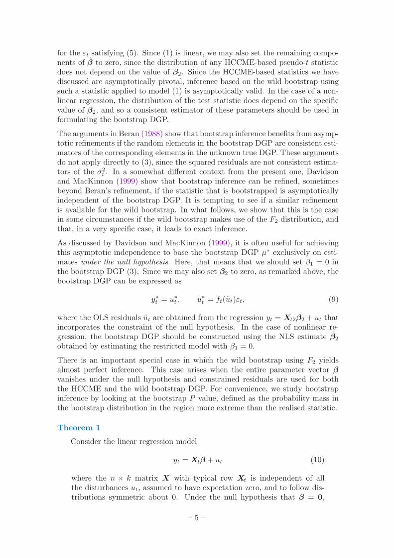
for the εt satisfying (5). Since (1) is linear, we may also set the remaining compo-nents of β to zero, since the distribution of any HCCME-based pseudo-t statisticdoes not depend on the value of β2. Since the HCCME-based statistics we havediscussed are asymptotically pivotal, inference based on the wild bootstrap usingsuch a statistic applied to model (1) is asymptotically valid. In the case of a non-linear regression, the distribution of the test statistic does depend on the specificvalue of β2, and so a consistent estimator of these parameters should be used informulating the bootstrap DGP.

The arguments in Beran (1988) show that bootstrap inference benefits from asymp-totic refinements if the random elements in the bootstrap DGP are consistent esti-mators of the corresponding elements in the unknown true DGP. These argumentsdo not apply directly to (3), since the squared residuals are not consistent estima-tors of the σ2

t . In a somewhat different context from the present one, Davidsonand MacKinnon (1999) show that bootstrap inference can be refined, sometimesbeyond Beran’s refinement, if the statistic that is bootstrapped is asymptoticallyindependent of the bootstrap DGP. It is tempting to see if a similar refinementis available for the wild bootstrap. In what follows, we show that this is the casein some circumstances if the wild bootstrap makes use of the F2 distribution, andthat, in a very specific case, it leads to exact inference.

As discussed by Davidson and MacKinnon (1999), it is often useful for achievingthis asymptotic independence to base the bootstrap DGP µ∗ exclusively on esti-mates under the null hypothesis. Here, that means that we should set β1 = 0 inthe bootstrap DGP (3). Since we may also set β2 to zero, as remarked above, thebootstrap DGP can be expressed as

y∗t = u∗t , u∗t = ft(ut)εt, (9)

where the OLS residuals ut are obtained from the regression yt = Xt2β2 + ut thatincorporates the constraint of the null hypothesis. In the case of nonlinear re-gression, the bootstrap DGP should be constructed using the NLS estimate β2

obtained by estimating the restricted model with β1 = 0.

There is an important special case in which the wild bootstrap using F2 yieldsalmost perfect inference. This case arises when the entire parameter vector βvanishes under the null hypothesis and constrained residuals are used for boththe HCCME and the wild bootstrap DGP. For convenience, we study bootstrapinference by looking at the bootstrap P value, defined as the probability mass inthe bootstrap distribution in the region more extreme than the realised statistic.

Theorem 1

Consider the linear regression model

yt = Xtβ + ut (10)

where the n × k matrix X with typical row Xt is independent of allthe disturbances ut, assumed to have expectation zero, and to follow dis-tributions symmetric about 0. Under the null hypothesis that β = 0,

– 5 –

the χ2 statistic for a test of that null against the alternative representedby (10), based on any of the four HCCMEs considered here constructedwith constrained residuals, has exactly the same distribution as the samestatistic bootstrapped, if the bootstrap DGP is the wild bootstrap (9),with f(u) = u or equivalently f(u) = |u|, for which the εt are generatedby the symmetric two-point distribution F2 of (7).

For sample size n, the bootstrap P value p∗ follows a discrete distributionsupported by the set of points pi = i/2n, i = 0, . . . , 2n − 1, with equalprobability mass 2−n on each point. For each nominal level α equal toone of the dyadic numbers 1/2n, i = 0, 1, . . . , 2n−1, the probability underthe null hypothesis that the bootstrap P value is less than α, that is, theprobability of Type I error at level α, is exactly equal to α

Proof:

The OLS estimates from (10) are given by β = (X>X)−1X>y, and any of theHCCMEs we consider for β can be written in the form (2), with an appropriatechoice of Ω. The χ2 statistic thus takes the form

τ ≡ y>X(X>ΩX)−1X>y. (11)

Under the null, y = u, and each component ut of u can be written as |ut|st, wherest, equal to ±1, is the sign of ut, and is independent of |ut| because we assume thatut follows a symmetric distribution. Define the 1× k row vector Zt as |ut|Xt, andthe n×1 column vector s with typical element st. The entire n×k matrix Z withtypical row Zt is then independent of the vector s. If the constrained residuals,which are just the elements of y, are used to form Ω, the statistic (11) is equal to

s>Z

(n∑

t=1

atZt>Zt

)−1

Z>s, (12)

where at is equal to 1 for HC0, n/(n − k) for HC1, 1/(1 − ht) for HC2, and1/(1− ht)2 for HC3.

If we denote by τ∗ the statistic generated by the wild bootstrap with F2, then τ∗

can be written as

ε>Z

(n∑

t=1

atZt>Zt

)−1

Z>ε, (13)

where ε denotes the vector containing the εt. The matrix Z is exactly the sameas in (12), because the exogenous matrix X is reused unchanged by the wildbootstrap, and the wild bootstrap disturbance terms u∗t = ±ut, since, under F2,εt = ±1. Thus, for all t, |u∗t | = |ut|. By construction, ε and Z are independentunder the wild bootstrap DGP. But it is clear that s follows exactly the samedistribution as ε, and so it follows that τ under the null and τ∗ under the wildbootstrap DGP with F2 have the same distribution. This proves the first assertionof the theorem.

– 6 –

Conditional on the |ut|, this common distribution of τ and τ∗ is of course a discretedistribution, since ε and s can take on only 2n different, equally probable, values,with a choice of +1 or −1 for each of the n components of the vector. In fact, thereare normally only 2n−1 different values, because, given that (13) is a quadraticform in ε, the statistic for −ε is the same as for ε. However, if there is only onedegree of freedom, one may take the signed square root of (13), in which case thesymmetry is broken, and the number of possible values is again equal to 2n. Forthe rest of this proof, therefore, we consider the case with 2n possibilities.

The statistic τ must take on one of these 2n possible values, each with the sameprobability of 2−n. If we denote the 2n values, arranged in increasing order, asτi, i = 1, . . . , 2n, with τj > τi for j > i, then, if τ = τi, the bootstrap P value,which is the probability mass in the distribution to the right of τi, is just 1− i/2n.As i ranges from 1 to 2n, the P value varies over the set of points pi ≡ i/2n,i = 0, . . . , 2n − 1, all with probability 2−n. This distribution, conditional onthe |ut|, does not depend on the |ut|, and so is also the unconditional distributionof the bootstrap P value.

For nominal level α, the bootstrap test rejects if the bootstrap P value is lessthan α. To compute this probability, we consider the rank i of the realised statis-tic τ in the set of 2n possibilities as a random variable uniformly distributed overthe values 1, . . . , 2n. The bootstrap P value, equal to 1− i/2n, is less than α if andonly if i > 2n(1 − α), an event of which the probability is 2−n times the numberof integers in the range b2n(1 − α)c + 1, . . . 2n, where bxc denotes the greatestinteger not greater than x. Let the integer k be equal to b2n(1 − α)c. Then theprobability we wish to compute is 2−n(2n − k) = 1− k2−n.

Suppose first that this probability is equal to α. Then α2n is necessarily an integer,so that α is one of the dyadic numbers mentioned in the statement of the theorem.Suppose next that α = j/2n, j an integer. Then b2n(1 − α)c = 2n − j, so thatk = 2n−j. The probability of rejection by the bootstrap test at level α is therefore1− k2−n = j/2n = α. This proves the final assertions of the Theorem.

Remarks: For small enough n, it may be quite feasible to enumerate all thepossible values of the bootstrap statistic τ∗, and thus obtain the exact value ofthe realisation p∗.

Although the discrete nature of the bootstrap distribution means that it is notpossible to perform exact inference for an arbitrary significance level α, the prob-lem is no different from the problem of inference with any discrete-valued statistic.For the case with n = 10, which will be extensively treated in the following sec-tions, 2n = 1024, and so the bootstrap P value cannot be in error by more than1 part in a thousand.

It is possible to imagine a case in which the discreteness problem is aggravated bythe coincidence of some adjacent values of the τi of the proof of the theorem. Forinstance, if the only regressor in X is the constant, the value of (12) depends onlyon the number of positive components of s and not on their ordering. For thiscase, of course, it is not necessary to base inference on an HCCME. Coincidence ofvalues of the τi will otherwise occur if all the explanatory variables take on exactlythe same values for more than one observation. However, since this phenomenon

– 7 –

is observable, it need not be a cause for concern. A very small change in the valuesof the components of the Xt would be enough to break the ties in the τi.

The exact result of the theorem is specific to the wild bootstrap with F2. Theproof works because the signs in the vector s also follow the distribution F2.Given the exact result of the theorem, it is of great interest to see the extentof the size distortion of the F2 bootstrap with constrained residuals when thenull hypothesis involves only a subset of the regression parameters. This questionwill be investigated by simulation in the following section. At this stage, it ispossible to see why the theorem does not apply more generally. The expressions(12) and (13) for τ and τ∗ continue to hold if the constrained residuals ut areused for Ω, and if Zt is redefined as |ut|(M2X1)t, where X1 is the matrix ofregressors admitted only under the alternative, and M2 is the projection off thespace spanned by the regressors that are present under the null. However, althoughε in τ∗ is by construction independent of Z, s in τ is not. This is because thecovariance matrix of the residual vector u is not diagonal in general, unlike thatof the disturbances u. In Figure 1, this point is illustrated for the bivariate case.In panel a), two level curves are shown of the joint density of two symmetricallydistributed and independent variables u1 and u2. In panel b), the two variables areno longer independent. For the set of four points for which the absolute values ofu1 and u2 are the same, it can be seen that, with independence, all four points lieon the same level curve of the joint density, but that this is no longer true withoutindependence. The vector of absolute values is no longer independent of the vectorof signs, even though independence still holds for the marginal distribution of eachvariable. Of course the asymptotic distributions of τ and τ∗ still coincide.

3. Experimental Design and Simulation Results

It was shown by Chesher and Jewitt (1987) that HCCMEs are most severelybiased when the regression design has observations with high leverage, and thatthe extent of the bias depends on the amount of heteroskedasticity in the true DGP.Since in addition one expects bootstrap tests to behave better in large samplesthan in small, in order to stress-test the wild bootstrap, most of our experimentsare performed with a sample of size 10 containing one regressor, denoted x1,all the elements but one of which are independent drawings from N(0, 1), butthe second of which is 10, so as to create an observation with exceedingly highleverage. All the tests we consider are of the null hypothesis that β1 = 0 in themodel (1), with k, the total number of regressors, varying across experiments. Inall regression designs, x1 is always present; for the design we designate by k = 2 aconstant, denoted x2, is also present; and for k = 3, . . . , 6, additional regressors xi,i = 3, . . . , 6 are successively appended to x1 and x2. In Table 1, the componentsof x1 are given, along with those of the xi, i = 3, . . . , 6. In Table 2 are given thediagonal elements ht of the orthogonal projections on to spaces spanned by x1, x1

and x2, x1, x2, and x3, etc. The ht measure the leverage of the 10 observationsfor the different regression designs.

The data in all the simulation experiments discussed here are generated underthe null hypothesis. Since (1) is a linear model, we set β2 = 0 without loss of

– 8 –

generality. Thus our data are generated by a DGP of the form

yt = σtvt, t = 1, . . . , n, (14)

where n is the sample size, 10 for most experiments. For homoskedastic data, weset σt = 1 for all t, and for heteroskedastic data, we set σt = |xt1|, the absolutevalue of the tth component of x1. Because of the high leverage observation, thisgives rise to very strong heteroskedasticity, which leads to serious bias of the OLScovariance matrix; see White (1980). The vt are independent variables of zeroexpectation and unit variance, and in the experiments will be either normal or elsedrawings from the highly skewed χ2(2) distribution, centred and standardised.

The main object of our experiments is to compare the size distortions of wildbootstrap tests using the distributions F1 and F2. Although the latter gives ex-act inference only in a very restricted case, we show that it always leads to lessdistortion than the former in sample sizes up to 100. We also conduct a few ex-periments comparing the wild bootstrap and the (y, X) bootstrap. In order toconduct a fair comparison, we use an improved version of the (y, X) bootstrapsuggested by Mammen (1993), and subsequently modified by Flachaire (1999), inwhich we resample, not the (y,X) pairs as such, but rather regressors (X) and theconstrained residuals, transformed according to HC3. For the wild bootstrap, weare also interested in the impact on errors in the rejection probabilities (ERPs) ofthe use of unconstrained versus constrained residuals, and the use of the differentsorts of HCCME. Here, we formally define the error in rejection probability as thedifference between the rejection probability, as estimated by simulation, at a givennominal level, and that nominal level.

We present our results as P value discrepancy plots, as described in Davidson andMacKinnon (1998). These plots show ERPs as a function of the nominal level α.Since we are considering a one-degree-of-freedom test, it is possible to perform aone-tailed test for which the rejection region is the set of values of the statisticalgebraically greater than the critical value. We choose to look at one-tailed testsbecause Edgeworth expansions predict – see Hall (1992) – that the ERPs of one-tailed bootstrap tests converge to zero with increasing sample size more slowlythan those of two-tailed tests. In any event, it is easy to compute the ERP of atwo-tailed test with the information in the P value discrepancy plot. All plots arebased on experiments using 100, 000 replications.

We now present our results as answers to a series of pertinent questions.• In a representative case, with strong heteroskedasticity and high leverage, is

the wild bootstrap capable of reducing the ERP relative to asymptotic tests?Figure 2 shows plots for the regression design with k = 3, sample size n = 10,and normal heteroskedastic disturbances. The ERPs are plotted for the conven-tional t statistic, based on the OLS covariance matrix estimate, the four versionsof HCCME-based statistics, HCi, i = 0, 1, 2, 3, all using constrained residuals.P values for the asymptotic tests are obtained using Student’s t distribution with7 degrees of freedom. The ERP is also plotted for what will serve as a base case forthe wild bootstrap: Constrained residuals are used both for the HCCME and thewild bootstrap DGP, the F2 distribution is used for the εt, and the statistic that

– 9 –

is bootstrapped is the HC3 form. To avoid redundancy, the plots are drawn onlyfor the range 0 ≤ α ≤ 0.5, since all these statistics are symmetrically distributedwhen the disturbances are symmetric. In addition, the bootstrap statistics aresymmetrically distributed conditional on the original data, and so the distribu-tion of the bootstrap P value is also symmetrical about α = 0.5. It follows thatthe ERP for nominal level α is the negative of that for 1 − α. Not surprisingly,the conventional t statistic, which does not have even an asymptotic justification,is the worst behaved of all, with far too much mass in the tails. But, althoughthe HCi statistics are less distorted, the bootstrap test is manifestly much betterbehaved.• The design with k = 1 satisfies the conditions of Theorem 1 when the dis-

turbances are symmetric and the HCCME and the bootstrap DGP are basedon constrained residuals. If we maintain all these conditions but consider thecases with k > 1, bootstrap inference is no longer perfect. To what extent isinference degraded?

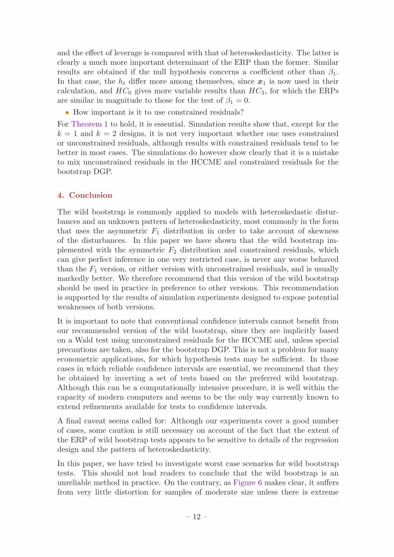
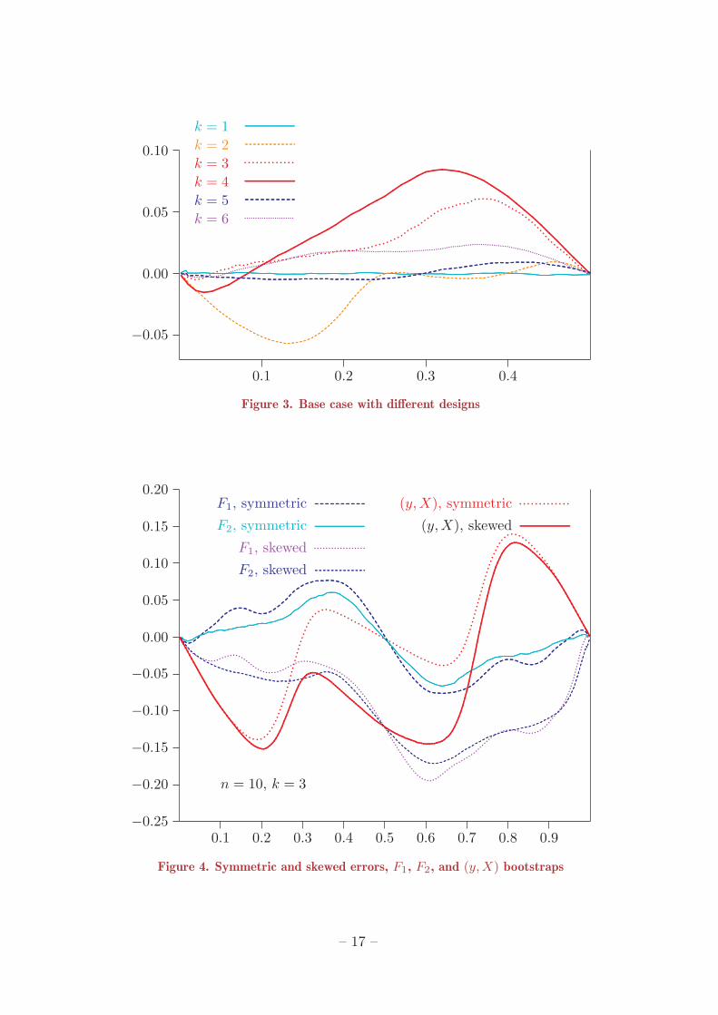
P value discrepancy plots are shown in Figure 3 for the designs k = 1, . . . , 6 usingthe base-case wild bootstrap as described above. Disturbances are normal andheteroskedastic. As expected, the ERP for k = 1 is just experimental noise, andfor most other cases the ERPs are significant. By what is presumably a coincidenceinduced by the specific form of the data, they are not at all large for k = 5 ork = 6. In any case, we can conclude that the ERP does indeed depend on theregression design, but quantitatively not very much, given the small sample size.• How do bootstrap tests based on the F1 and F2 distributions compare? We

expect that F2 will lead to smaller ERPs if the disturbances are symmetric,but what if they are asymmetric? How effective is the skewness correctionprovided by F1? What about the (y,X) bootstrap?

In Figure 4 plots are shown for the k = 3 design with heteroskedastic normaldisturbances and skewed χ2(2) disturbances. The F1 and F2 bootstraps give rathersimilar ERPs, whether or not the disturbances are skewed. But the F2 bootstrap isgenerally better, and never worse. Very similar results, leading to same conclusion,were also obtained with the k = 4 design. For k = 1 and k = 2, on the otherhand, the F1 bootstrap suffers from larger ERPs than for k > 2. Plots are alsoshown for the same designs and the preferred form of the (y, X) bootstrap. It isclear that the ERPs are quite different from those of the wild bootstrap, in eitherof its forms, and substantially greater.• What is the penalty for using the wild bootstrap when the disturbances are

homoskedastic and inference based on the conventional t statistic is reliable,at least with normal disturbances? Do we get different answers for F1, F2,and the (y, X) bootstrap?

Again we use the k = 3 design. We see from Figure 5, which is like Figure 4 ex-cept that the disturbances are homoskedastic, that, with normal disturbances, theERP is very slight with F2, but remains significant for F1 and (y,X). Thus, withunskewed, homoskedastic disturbances, the penalty attached to using the F2 boot-strap is very small. With skewed disturbances, all three tests give substantiallygreater ERPs, but the F2 version remains a good deal better than the F1 version,which in turn is somewhat better than the (y, X) bootstrap.

– 10 –

• Do the rankings of bootstrap procedures obtained so far for n = 10 continueto apply for larger samples? Do the ERPs become smaller rapidly as n grows?

In order to deal with larger samples, the data in Table 1 were simply repeatedas needed in order to generate regressors for n = 20, 30, . . .. The plots shownin Figures 4 and 5 are repeated in Figure 6 for n = 100. The rankings foundfor n = 10 remain unchanged, but the ERP for the F2 bootstrap with skewed,heteroskedastic, disturbances improves less than that for the F1 bootstrap withthe increase in sample size. It is noteworthy that none of the ERPs in this diagramis very large.

In Figure 7, we plot the ERP for α = 0.05 as a function of n, n = 10, 20, . . .,with the k = 3 design and heteroskedastic disturbances, normal for F1 andskewed for F2, chosen because these configurations lead to comparable ERPs forn around 100, and because this is the worst setup for the F2 bootstrap. It isinteresting to observe that, at least for α = 0.05, the ERPs are not monotonic.What seems clear is that, although the absolute magnitude of the ERPs is not dis-turbingly great, the rate of convergence to zero does not seem to be at all rapid,and seems to be slower for the F2 bootstrap.

We now move on to consider some lesser questions, the answers to whichjustify, at least partially, the choices made in the design of our earlier experiments.We restrict attention to the F2 bootstrap, since it is clearly the procedure of choicein practice.• Does it matter which of the four versions of the HCCME is used?

It is clear from Figure 2 that the choice of HCi has a substantial impact on theERP of the asymptotic test. Since the HC0 and HC1 statistics differ only by aconstant multiplicative factor, they yield identical bootstrap P values, as do allversions for k = 1 and k = 2. For k = 1 this is obvious, since the raw statisticsare identical, and for k = 2, the only regressor other than x1 is the constant, andso ht does not depend on t. For k > 2, significant differences appear, as seen inFigure 8 which treats the k = 4 design. HC3 has the least distortion here, andalso for the other designs with k > 2. This accounts for our choice of HC3 in thebase case.• What is the best transformation ft(·) to use in the definition of the bootstrap

DGP? Plausible answers are either the identity transformation, or the sameas that used for the HCCME.

No very clear answer to this question emerged from our numerous experiments onthis point. A slight tendency in favour of using the HC3 transformation appears,but this choice does not lead to universally smaller ERPs. However, the quanti-tative impact of the choice is never very large, and so the HC3 transformation isused in our base case.• How is performance affected if the leverage of observation 2 is reduced?

Because the ERPs of the asymptotic tests are greater with a high leverage observa-tion, we might expect the same to be true of bootstrap tests. In fact, although thisis true if the HC0 statistic is used, the use of widely varying ht with HC3 providesa good enough correction that, with it, the presence or absence of leverage has lit-tle impact. In Figure 9, this is demonstrated for k = 3, and normal disturbances,

– 11 –

and the effect of leverage is compared with that of heteroskedasticity. The latter isclearly a much more important determinant of the ERP than the former. Similarresults are obtained if the null hypothesis concerns a coefficient other than β1.In that case, the ht differ more among themselves, since x1 is now used in theircalculation, and HC0 gives more variable results than HC3, for which the ERPsare similar in magnitude to those for the test of β1 = 0.• How important is it to use constrained residuals?

For Theorem 1 to hold, it is essential. Simulation results show that, except for thek = 1 and k = 2 designs, it is not very important whether one uses constrainedor unconstrained residuals, although results with constrained residuals tend to bebetter in most cases. The simulations do however show clearly that it is a mistaketo mix unconstrained residuals in the HCCME and constrained residuals for thebootstrap DGP.

4. Conclusion

The wild bootstrap is commonly applied to models with heteroskedastic distur-bances and an unknown pattern of heteroskedasticity, most commonly in the formthat uses the asymmetric F1 distribution in order to take account of skewnessof the disturbances. In this paper we have shown that the wild bootstrap im-plemented with the symmetric F2 distribution and constrained residuals, whichcan give perfect inference in one very restricted case, is never any worse behavedthan the F1 version, or either version with unconstrained residuals, and is usuallymarkedly better. We therefore recommend that this version of the wild bootstrapshould be used in practice in preference to other versions. This recommendationis supported by the results of simulation experiments designed to expose potentialweaknesses of both versions.

It is important to note that conventional confidence intervals cannot benefit fromour recommended version of the wild bootstrap, since they are implicitly basedon a Wald test using unconstrained residuals for the HCCME and, unless specialprecautions are taken, also for the bootstrap DGP. This is not a problem for manyeconometric applications, for which hypothesis tests may be sufficient. In thosecases in which reliable confidence intervals are essential, we recommend that theybe obtained by inverting a set of tests based on the preferred wild bootstrap.Although this can be a computationally intensive procedure, it is well within thecapacity of modern computers and seems to be the only way currently known toextend refinements available for tests to confidence intervals.

A final caveat seems called for: Although our experiments cover a good numberof cases, some caution is still necessary on account of the fact that the extent ofthe ERP of wild bootstrap tests appears to be sensitive to details of the regressiondesign and the pattern of heteroskedasticity.

In this paper, we have tried to investigate worst case scenarios for wild bootstraptests. This should not lead readers to conclude that the wild bootstrap is anunreliable method in practice. On the contrary, as Figure 6 makes clear, it suffersfrom very little distortion for samples of moderate size unless there is extreme

– 12 –

heteroskedasticity. In most practical contexts, use of the F2-based wild bootstrapwith constrained residuals should provide satisfactory inference.

References

Beran, R. (1986). Discussion of “Jackknife bootstrap and other resamplingmethods in regression analysis” by C. F. J. Wu., Annals of Statistics 14,1295–1298.

Beran, R. (1988). “Prepivoting test statistics: a bootstrap view of asymptoticrefinements”, Journal of the American Statistical Association, 83, 687–697.

Bhattacharya, R. N., and J. K. Ghosh (1978). “On the validity of the formalEdgeworth expansion”, Annals of Statistics, 6, 434–451.

Chesher A. and I. Jewitt (1987). “The bias of a heteroskedasticity consistentcovariance matrix estimator”, Econometrica, 55, 1217–1222.

Davidson, R. and E. Flachaire (2001). “The Wild Bootstrap, Tamed at Last”,Queen’s Economics Department working paper #1000, Queen’s University,Kingston, Canada.

Davidson, R. and J. G. MacKinnon (1998). “Graphical methods for investigatingthe size and power of hypothesis tests”, The Manchester School, 66, 1–26.

Davidson, R. and J. G. MacKinnon (1999). “The size distortion of bootstraptests”, Econometric Theory, 15, 361–376.

Eicker, F. (1963). “Asymptotic normality and consistency of the least squaresestimators for families of linear regressions”, The Annals of MathematicalStatistics, 34, 447–456.

Feller, W. (1971). An Introduction to Probability Theory and its Applications,second edition, Wiley, New York.

Flachaire, E. (1999). “A better way to bootstrap pairs”, Economics Letters, 64,257–262.

Freedman, D. A. (1981). “Bootstrapping regression models”, Annals ofStatistics, 9, 1218–1228.

Hall, P. (1992). The Bootstrap and Edgeworth Expansion, Springer-Verlag, NewYork.

Kolassa, J. E. (1994). Series Approximations in Statistics, Lecture Notes inStatistics 88, Springer-Verlag, New York.

Liu, R. Y. (1988). “Bootstrap procedures under some non-I.I.D. models”, Annalsof Statistics 16, 1696–1708.

– 13 –

MacKinnon, J. G., and H. White (1985). “Some heteroskedasticity consistentcovariance matrix estimators with improved finite sample properties”, Journalof Econometrics, 29, 305–325.

Mammen, E. (1993). “Bootstrap and wild bootstrap for high dimensional linearmodels”, Annals of Statistics 21, 255–285.

White, H. (1980). “A heteroskedasticity-consistent covariance matrix estimatorand a direct test for heteroskedasticity”, Econometrica, 48, 817–838.

Wu, C. F. J. (1986). “Jackknife bootstrap and other resampling methods inregression analysis”, Annals of Statistics 14, 1261–1295.

– 14 –

Table 1. Regressors

Obs x1 x3 x4 x5 x6

1 0.616572 0.511730 0.210851 -0.651571 0.509960

2 10.000000 5.179612 4.749082 6.441719 1.212823

3 -0.600679 0.255896 -0.150372 -0.530344 0.318283

4 -0.613076 0.705476 0.447747 -1.599614 -0.601335

5 -1.972106 -0.673980 -1.513501 0.533987 0.654767

6 0.409741 0.922026 1.162060 -1.328799 1.607007

7 -0.676614 0.515275 -0.241203 -1.424305 -0.360405

8 0.400136 0.459530 0.166282 0.040292 -0.018642

9 1.106144 2.509302 0.899661 -0.188744 1.031873

10 0.671560 0.454057 -0.584329 1.451838 0.665312

Table 2. Leverage measures

Obs k = 1 k = 2 k = 3 k = 4 k = 5 k = 6

1 0.003537 0.101022 0.166729 0.171154 0.520204 0.560430

2 0.930524 0.932384 0.938546 0.938546 0.964345 0.975830

3 0.003357 0.123858 0.128490 0.137478 0.164178 0.167921

4 0.003497 0.124245 0.167158 0.287375 0.302328 0.642507

5 0.036190 0.185542 0.244940 0.338273 0.734293 0.741480

6 0.001562 0.102785 0.105276 0.494926 0.506885 0.880235

7 0.004260 0.126277 0.138399 0.143264 0.295007 0.386285

8 0.001490 0.102888 0.154378 0.162269 0.163588 0.218167

9 0.011385 0.100300 0.761333 0.879942 0.880331 0.930175

10 0.004197 0.100698 0.194752 0.446773 0.468841 0.496971

Notes: For k = 1, the only regressor is x1, for k = 2 there is also the constant, fork = 3 there are the constant, x1, and x2, and so forth.

– 15 –

.............................................................................................................................................................................................................................................................................................. ............

.......

........

.......

.......

.......

........

.......

.......

........

.......

.......

.......

........

.......

.......

.......

........

.......

.......

........

.......

.......

.......

........

.......

.......

.......

........

.......

.......

.......

........

.......

.......

........

.......

.......

.................

............

..........................

............................

............................................................................................................................................................................................................................................................................................................................................................

..................................

................................ ........

...........................

...........................

.......................................................

............................................................................................................................................................................................................................................................................................................................................................................................................

..................................................................

•

•

•

•u1

u2

.............................................................................................................................................................................................................................................................................................. ............

.......

........

.......

.......

.......

........

.......

.......

........

.......

.......

.......

........

.......

.......

.......

........

.......

.......

........

.......

.......

.......

........

.......

.......

.......

........

.......

.......

.......

........

.......

.......

........

.......

.......

.................

............

..................................................................................................................................................................................................................................................................................................................

.....................

.......................

................................

............................................

...................................................................................................................................................................................................................................................................................................................................................................................................................................................................................................................

....................

....................

......................

.........................

.............................

.................................................

............................................

•

•

•

•u1

u2

Figure 1. Absolute values and signs of two random variables

0.1 0.2 0.3 0.4

−0.2

−0.1

0.0

0.1

0.2

0.3

.........................................................................................................................................................................................................................................................................................

...............................................................................................

............................................................................................................................................................................................................................................

.....................................................................Wild bootstrap (HC3)

..............................................................................................................................

.........................................................................................................................................................

.......................HC0

......................................................................................................................................................

.............HC1

................................................................................................................................................................................................................................................................................................................................................................................................................................................................................................................................................................................................................................................................

.......................................................................................................................................................................................................................................................................................................................................................................................................................................................................................................................................................................................

....................................................................................................HC2

...........................................................................................................................................................................................................................................................................................................................................................................................................................................................................................................................................................................................................................................................................................................................................................................................................................................................................................................................................................................

................................................................................HC3

.................

.................

.................

.................

.................

.................

.................

.................

.................

.................

..................

.................

.................

.................

.................

.................

.................

.................

..................

.................

.................

.................

..................

.................

.................

.................

..................

.................

..............................................................................................................................................................................................................................................................................

............................................................................................................................................................................................................................................................................................................................................................................................................................................................................................................................................................................................................................................................................................................................................................................................................................................................................................................................................................................................................................................................................................................................................................................................................................................................................................................................................................................................................................................................................................................................................................................................................................................................................................................

..............................................................................................................................................................................................t statistic

n = 10, k = 3

Figure 2. ERPs of asymptotic and bootstrap tests

– 16 –

0.1 0.2 0.3 0.4

−0.05

0.00

0.05

0.10

..................................................................................................................................................................................................................................................................................................................................................................................................................................................................................................................................................................................................................................................................................................................................................................................................................................................................................................................................................................................................................................................................................................................................................................................................................................................................................................................................................................................................................................................................................................................................................................................................................................................................

..............................................................................................................................................................................................k = 1

..................................................................................................................................................................................................................................................................................................................................

.........................................................................................................................................................................................

............................................................................................................................................................................................................................................................................

.................................................................................................................................................

....................................................................................................k = 2

.........................

.............................

..........

...........

........................................

.............k = 3

................................................................................................................

..................................................

......................................................

.....................................................

...................................................

................................................

........................................................................................................................................................................................................................................................................................................................................

.....................................................................k = 4

........................................................................................................................................................................................................................................................................................................................................................................................................................

........................................................................................................................................................................................................................................

...............................................................................k = 5

...................................

......................

.......................................................................

..................................................................

.......................k = 6

Figure 3. Base case with different designs

0.1 0.2 0.3 0.4 0.5 0.6 0.7 0.8 0.9−0.25

−0.20

−0.15

−0.10

−0.05

0.00

0.05

0.10

0.15

0.20

..............................................................................................................................................................................

..................................................

........................................................................................................................................................................................................................................................................................................................................................

......................................................................

..........................................................................................................

................................

...................

...............................................................................F1, symmetric

............................................................................................................................

.....................................................................................................................................................................................................................

..............................................................................................................................

................................................................................................................................

..................................................................................................................................................................................................................................................................................................................................................................................................................................................................................................................................................................................................................................................................................................................................................................................................................................

....................................................................

.........................................................................................................................................................................................................

....................................................................................

...................................................................................................................................

..............................................................................................................................................................................................F2, symmetric

............................................

.............................................................................

........

...........

.......................................................

..................F1, skewed

.......................................................................................................................................................................................................................................................................................................................

...........................................................................................................................................................................................................................................................................................................................................................

....................................

..........................................

.............................................................................

...........................................

........................................................................................................................................................................................

....................................................................................................F2, skewed

..............................................................................................................

..................................

..................................

.............(y, X), symmetric

.....................................................................................................................................................................................................................................................................................................................................................................................................................................................................................................................................................................................................................................

..............................................................................................................................................................................................................................................................................................................................................................................................................................................................................................................

.....................................................................(y, X), skewed

n = 10, k = 3

Figure 4. Symmetric and skewed errors, F1, F2, and (y, X) bootstraps

– 17 –

0.1 0.2 0.3 0.4 0.5 0.6 0.7 0.8 0.9−0.10

−0.05

0.00

0.05

0.10

................................................................................

......................................................................................................................................................................................

..............................................................................................................................................................................................................

.............................

...............................................................................................................................................................................................................

...................................

...............................................................................F1, symmetric

...........................................................................................................................

.......................................................................................................................................................................................................................................................................................................................................................................................................................................................................................................................................................................................................................................................

...............................................................................................................................................................................................................................................................

.....................................................................................................................................................................................................................................................................................................................................................................................................................................................................................................................................................................................................................................................................................

..............................................................................................................................................................................................F2, symmetric

..............

........

.................................

..........

..............................................................................................

.........

..................F1, skewed

.......................................................................

.........................................................................................................................................................................................................................................................

........................................................

......................................................................................................................................................................................................................................................................................................................................................................................................................................................

................................

....................................................................................................F2, skewed

...................................................

.........

......................

..............................

.......................

.............(y, X), symmetric

....................................................................................................................................................................................

....................................................................................................................................................................................................

...................................................................................................................

......................................................................

....................................................................................................................................................................................................................................................

.....................................................................(y, X), skewed

n = 10, k = 3

Figure 5. Homoskedastic errors

0.1 0.2 0.3 0.4 0.5 0.6 0.7 0.8 0.9−0.25

−0.20

−0.15

−0.10

−0.05

0.00

0.05

0.10

........................................................................................................................................................................................................................................................................................................................................................................................................................................................................................................................................................................................................................................................................

........

...............................................................................F1, symmetric, heteroskedastic

..........................................................................................................................................................................................................................................................................................................................................................................................................................................................................................................................................................................................................................................................................................................................................................................................................................................................................................................................................................................................................................................................................................................................................................................................................................................................................................................................................................................................................................................................................................................................................................................................................................................................................

..............................................................................................................................................................................................F2, symmetric, heteroskedastic

..........................................................................................................................................................................................................................................................................

...........................................................................................................................................................................................................................................................................................................................................................................................................................................................................................................................................................................................................................................................

.....................................................

..................................................................................................F1, skewed, heteroskedastic

..........................................................................

.....................................................................................

..................F2, skewed, heteroskedastic

..........................................................................................................

.............F1, symmetric, homoskedastic

................................................................................................................................................................................................................................................................................................................................................................................................................................................................................................................................................................................................................................................................................................................................................................................................................................................

....................................................................................................F2, symmetric, homoskedastic

...................................................................................................................................................................................................................................................................................................................................................................................................................................................................................................................................................................................................................................................

..........................................................................F1, skewed, homoskedastic

..........

...............................................................................................................................

..........................................................

.......................F2, skewed, homoskedasticn = 100, k = 3

Figure 6. ERPs for n = 100

– 18 –

10 20 30 40 50 60 70 80 90 100−0.10

−0.05

0.00

0.05

0.10

••

• • • • • • • •

• •F2, skewed

F1, symmetric

Figure 7. ERP for nominal level 0.05 as function of sample size

0.1 0.2 0.3 0.4−0.05

0.00

0.05

0.10

0.15

0.20

......................................................................................................................................................................................................................................................................................................................................................................................................................................................................................................................................................................................................................................................................................................................................................................................................................................................................................................................................................................................................................................................................................................................................................................................................................................................................................................................................................................................................................................................................................................................................................................................................................................................................................................................................................................................................................................................................................................................................

...............................................................................................

............................................................................................................................................................................................................................................

.....................................................................HC3

...............................................................................................................................................................................................................................................................................................

............................................................................................................................................................................................................................................................................................................................................................................................................................................................................................................................................................................................................................................................................................................

....................................................................................................HC0

.....................

.........

..........................................................................................

.............HC2

n = 10, k = 3

Figure 8. HC3 compared with HC0 and HC2

– 19 –

0.1 0.2 0.3 0.4−0.04

−0.02

0.00

0.02

0.04

0.06

0.08

0.10

0.12

0.14

0.16

0.18

.....................................................................................................................

....................................................................................................................................................................................

...........................................................

.................................................

...............................................................................................................................................................................................................................................................

..............................................HC3, hetero, leverage

.....................................

........

...................

.........

...................................................

.........HC3, hetero, no leverage

.........................................................................................................................................................

.........................................................................................................................................................................................................................................................................................................................................................................................................................................................................................................................................................................................................................................................................................................................................................................................................................................................................................................................................................................................................................................................................................................................................

..........................................................................................................................................................................................................................

..............................................................................................................................................................

...............................................................................................................................HC3, homo, leverage

...............................................................................................................................................................................................

................HC3, homo, no leverage

........................................................................................................................................................................................................................................................................................................................................................................

.................................................................................................................................................................................................................................................................................................................................................................................................................................................................................................................................................................................................................................

.....................................................HC0, hetero, leverage

................................................

........

...............................

........

...........

...............................................................

............HC0, hetero, no leverage

n = 10, k = 3

Figure 9. Relative importance of leverage and heteroskedasticity

– 20 –