the weibull-g family of probability distributions · the weibull-gfamily of probability...

Journal of Data Science 12(2014), 53-68

The Weibull-G Family of Probability Distributions

Marcelo Bourguignon∗, Rodrigo B. Silva and Gauss M. CordeiroUniversidade Federal de Pernambuco

Abstract: The Weibull distribution is the most important distribution forproblems in reliability. We study some mathematical properties of the newwider Weibull-G family of distributions. Some special models in the newfamily are discussed. The properties derived hold to any distribution in thisfamily. We obtain general explicit expressions for the quantile function, or-dinary and incomplete moments, generating function and order statistics.We discuss the estimation of the model parameters by maximum likelihoodand illustrate the potentiality of the extended family with two applicationsto real data.

Key words: Generalized distribution, lifetime, maximum likelihood estima-tion, order statistic, Weibull distribution.

1. Introduction

Numerous classical distributions have been extensively used over the pastdecades for modeling data in several areas such as engineering, actuarial, environ-mental and medical sciences, biological studies, demography, economics, financeand insurance. However, in many applied areas such as lifetime analysis, financeand insurance, there is a clear need for extended forms of these distributions. Forthat reason, several methods for generating new families of distributions havebeen studied.

Some attempts have been made to define new families of probability distri-butions that extend well-known families of distributions and at the same timeprovide great flexibility in modeling data in practice. One such example is abroad family of univariate distributions generated from the Weibull distributionintroduced by Gurvich et al. (1997), by extending the classical Weibull model.Its cumulative distribution function (cdf) is given by

G(x;α, ξ) = 1− exp[−αH(x; ξ)], x ∈ D ⊆ R, α > 0, (1)

∗Corresponding author.

54 Marcelo Bourguignon, Rodrigo B. Silva and Gauss M. Cordeiro

where H(x; ξ) is a non-negative monotonically increasing function depending onthe parameter vector ξ.

The corresponding probability density function (pdf) becomes

g(x;α, ξ) = α exp[−αH(x; ξ)]h(x; ξ),

where h(x; ξ) is the derivative of H(x; ξ). Different functions H(x; ξ) in (1)include important statistical models such as: H(x; ξ) = x gives the exponentialdistribution; H(x; ξ) = x2 leads to the Rayleigh distribution; H(x; ξ) = log(x/k)yields the Pareto distribution; H(x; ξ) = β−1[exp(βx) − 1] gives the Gompertzdistribution.

Recently, Zografos and Balakrishnan (2009) proposed and studied a broadfamily of univariate distributions through a particular case of Stacy’s generalizedgamma distribution. Consider a continuous distribution G with density g, andfurther Stacy’s generalized gamma density f(x) = γxγ δ−1e−x

γ/Γ(δ) for x >

0 and positive parameters γ and δ. Based on this density, by replacing x by− log[1−G(x)] and considering γ = 1, Zografos and Balakrishnan (2009) definedtheir family with cdf

F (x; δ) = γ{δ,− log[1−G(x)]}, x ∈ X ⊆ R, δ > 0,

where γ(δ, z) =∫ z0 t

δ−1e−tdt/Γ(δ) denotes the incomplete gamma function andΓ(·) is the gamma function.

This pdf family is given by

f(x; δ) =1

Γ(δ){− log[1−G(x)]}δ−1 g(x).

The Weibull distribution is a very popular model and it has been extensivelyused over the past decades for modeling data in reliability, engineering and bio-logical studies. It is generally adequate for modeling monotone hazard rates. Inthis paper, we introduce and study in generality a family of univariate distribu-tions with two additional parameters, in the same vein as the extended Weibull(Gurvich et al., 1997) and gamma (Zografos and Balakrishnan, 2009) families,using the Weibull generator applied to the odds ratio G(x)/[1−G(x)]. The term“generator” means that for each baseline distribution G we have a different dis-tribution F . The main aim of this paper is to study a new family of distributions,with the hope it yields a “better fit” in certain practical situations. Addition-ally, we provide a comprehensive account of the mathematical properties of theproposed family of distributions.

This paper is unfolded as follows. In Section 2, we define the Weibull-Gfamily of distributions. Section 3 provides some special distributions obtainedby the Weibull generator. In Section 4, some general mathematical properties of

The Weibull-G Family of Probability Distributions 55

the family are discussed. The formulas derived are manageable by using moderncomputer resources with analytic and numerical capabilities. In Section 5, theestimation of the model parameters is performed by the method of maximumlikelihood. In Section 6, two illustrative applications based on real data areinvestigated. Finally, concluding remarks are presented in Section 7.

2. The Weibull-G Family of Distributions

Consider a continuous distribution G with density g and the Weibull cdfF (x) = 1 − e−αxβ (for x > 0) with positive parameters α and β. Based on thisdensity, by replacing x with G(x)/G(x) [G(x) = 1 − G(x)], we define the cdffamily by

F (x;α, β, ξ) =

∫ G(x;ξ)1−G(x;ξ)

0αβ tβ−1e−α t

βdt

= 1− exp

{−α

[G(x; ξ)

G(x; ξ)

]β}, x ∈ D ⊆ R; α, β > 0, (2)

where G(x; ξ) is a baseline cdf, which depends on a parameter vector ξ. Thefamily pdf reduces to

f(x;α, β, ξ) = αβ g(x; ξ)G(x; ξ)β−1

G(x; ξ)β+1exp

{−α

[G(x; ξ)

G(x; ξ)

]β}. (3)

Henceforth, let G be a continuous baseline distribution. For each G distri-bution, we define the Weibull-G (Wei-G for short) distribution with two extraparameters α and β defined by the pdf (3). A random variable X with pdf (3)is denoted by X ∼Wei-G(α, β, ξ). The additional parameters induced by theWeibull generator are sought as a manner to furnish a more flexible distribution.If β = 1, it corresponds to the exponential-generator.

An interpretation of the Wei-G family of distributions can be given as follows(Cooray, 2006) in a similar context. Let Y be a lifetime random variable havinga certain continuous G distribution. The odds ratio that an individual (or com-ponent) following the lifetime Y will die (failure) at time x is G(x; ξ)/G(x; ξ).Consider that the variability of this odds of death is represented by the randomvariable X and assume that it follows the Weibull model with scale α and shapeβ. We can write

Pr(Y ≤ x) = Pr

(X ≤ G(x; ξ)

G(x; ξ)

)= F (x;α, β, ξ),

which is given by (2).


The hazard rate function of the Wei-G family is given by

τ(x;α, β, ξ) =αβ g(x; ξ)G(x; ξ)β−1

G(x; ξ)β+1=αβ G(x; ξ)β−1

G(x; ξ)βτ(x; ξ),

where τ(x; ξ) = g(x; ξ)/G(x; ξ). The multiplying quantity αβ G(x; ξ)β−1/G(x; ξ)β

works as a corrected factor for the hazard rate function of the baseline model. (2)can deal with general situations in modeling survival data with various shapesof the hazard rate function. Table 1 lists G(x; ξ)/G(x; ξ) and the correspondingparameters for some special distributions.

Table 1: Distributions and corresponding G(x; ξ)/G(x; ξ) functions

Distribution G(x; ξ)/G(x; ξ) ξ

Uniform (0 < x < θ) x/(θ − x) θ

Exponential (x > 0) eλx − 1 λ

Weibull (x > 0) eλxγ − 1 (λ, γ)

Frechet (x > 0) (eλxγ − 1)−1 (λ, γ)

Half-logistic (x > 0) (ex − 1)/2 ∅Power function (0 < x < 1/θ) [(θ x)−k − 1]−1 (θ, k)

Pareto (x ≥ θ) (x/θ)k − 1 (θ, k)

Burr XII (x > 0) [1 + (x/s)c]k − 1 (s, k, c)

Log-logistic (x > 0) [1 + (x/s)c]− 1 (s, c)

Lomax (x > 0) [1 + (x/s)]k − 1 (s, k)

Gumbel (−∞ < x <∞) {exp[exp(−(x− µ)/σ)]− 1}−1 (µ, σ)

Kumaraswamy (0 < x < 1) (1− xa)−b − 1 (a, b)

Normal (−∞ < x <∞) Φ((x− µ)/σ)/(1− Φ((x− µ)/σ)) (µ, σ)

3. Examples

In this section, we give some examples of the Wei-G family of distributions.The pdf (3) will be most tractable when the cdf G(x; ξ) and the pdf g(x; ξ)have simple analytic expressions. These sub-models generalize several importantexisting distributions in the literature; for example, Phani, exponential power,Chen, among others distributions.

3.1 Weibull-Uniform Distribution

As a first example, suppose that the parent distribution is uniform in theinterval (0, θ), θ > 0. Then, g(x; θ) = 1/θ, 0 < x < θ < ∞ and G(x; θ) = x/θ.


The Weibull-Uniform (WU) has cdf given by

FWU(x;α, β, θ) = 1− exp

[−α

(x

θ − x

)β], 0 < x < θ <∞,

where α, β > 0. This distribution is known in the literature as the Phani distri-bution, see Phani (1987). The corresponding pdf is

fWU(x;α, β, θ) =θ α β

(θ − x)2

(x

θ − x

)β−1exp

[−α

(x

θ − x

)β], 0 < x < θ <∞.

3.2 Weibull-Weibull Distribution

As a second example, consider the power function distribution with densityand distribution functions (for x > 0) given by g(x;λ, γ) = λ γ xγ−1e−λx

γ, λ, γ >

0 and G(x;λ, γ) = 1− e−λxγ , respectively. Then, the Wei-Weibull (WW) distri-bution has cdf given by

FWW(x;α, β, λ, γ) = 1− exp[−α (eλx

γ − 1)β], x > 0.

The WW distribution includes the exponential power (Smith and Bain, 1975)distribution when β = 1 and α = 1. Further, for β = 1 and λ = 1, we obtain theChen (Chen, 2000) distribution. If β = γ = 1 and α = θ/λ (θ > 0), we obtainthe Gompertz (Gompertz, 1895) distribution. The corresponding pdf is

fWW(x;α, β, λ, γ) = αβ λγ xγ−1(1− e−λxγ)β−1 exp

{λβ xγ − α (eλx

γ − 1)β},

x > 0. (4)

3.3 Weibull-Burr XII Distribution

Let us consider the parent Burr XII distribution with pdf and cdf given byg(x) = ck s−cxc−1[1 + (x/s)c]−k−1, s, k, c > 0 and G(x) = 1 − [1 + (x/s)c]−k,respectively. Then, the Wei-BXII (WBXII) distribution has cdf given by

FWBXII(x;α, β, s, k, c) = 1− exp{−α [(1 + (x/s)c)k − 1]β

}, x > 0.

The WBXII distribution includes the generalized power Weibull (Nikulin andHaghighi, 2006) distribution when α = β = 1. The corresponding pdf (for x > 0)becomes

fWBXII(x;α, β, s, k, c) =αβck s−cxc−1

1 + (x/s)cexp

{−α [(1 + (x/s)c)k − 1]β

}×[(1 + (x/s)c)k − 1]β−1. (5)


3.4 Weibull-Normal Distribution

The last example refers to the normal distribution. The Wei-normal (WN)density is obtained from (3) by taking G(·) and g(·) to be the cdf and pdf of thenormal N(µ, σ2) distribution. Then, the WN distribution has cdf given by

FWN(x;α, β, µ, σ) = 1− exp

−α[

Φ(x−µ

σ

)1− Φ

(x−µσ

)]β , −∞ < x <∞,

where −∞ < µ <∞, σ > 0 and φ(·) and Φ(·) are the pdf and cdf of the standardnormal distribution, respectively. For µ = 0 and σ = 1, we obtain the standardWN distribution. The corresponding pdf is

fWN(x;α, β, µ, σ) =αβ φ

(x−µσ

)σ

Φ(x−µ

σ

)β−1[1− Φ

(x−µσ

)]β+1exp

−α[

Φ(x−µ

σ

)1− Φ

(x−µσ

)]β ,

−∞ < x <∞.

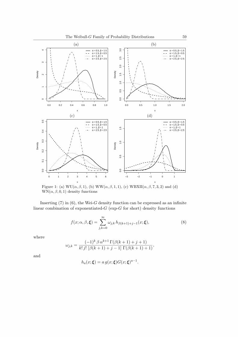
Figure 1 illustrates possible shapes of the density functions for some Weibull-G distributions.

4. Mathematical Properties

Despite the fact that the Wei-G cdf and pdf require mathematical functionsthat are widely available in modern statistical packages, frequently analytical andnumerical derivations take advantage of power series for the pdf. By using thepower series for the exponential function, we obtain

exp

{−α

[G(x; ξ)

G(x; ξ)

]β}=∞∑k=0

(−1)kαk

k!

[G(x; ξ)

G(x; ξ)

]k β.

Inserting this expansion in (2), we have

f(x;α, β, ξ) = αβ g(x; ξ)∞∑k=0

(−1)kαk

k!

G(x; ξ)β(k+1)−1

G(x; ξ)β(k+1)+1. (6)

Now, using the generalized binomial theorem, we can write

G(x; ξ)−[β(k+1)+1] =∞∑j=0

Γ(β(k + 1) + j + 1)

j! Γ(β(k + 1) + 1)G(x; ξ)j . (7)


(a) (b)

0.0 0.2 0.4 0.6 0.8 1.0

01

23

4

x

Den

sity

α = 0.5, β = 1.5α = 1.5, β = 0.5α = 1, β = 1α = 2.5, β = 2.5

0.0 0.5 1.0 1.5 2.0

0.0

0.5

1.0

1.5

2.0

2.5

3.0

x

Den

sity

α = 0.5, β = 1.5α = 1.5, β = 0.5α = 1, β = 1α = 2.5, β = 2.5

(c) (d)

0 1 2 3 4 5 6

0.0

0.1

0.2

0.3

0.4

0.5

x

Den

sity

α = 0.5, β = 1.5α = 1.5, β = 0.5α = 1, β = 1α = 2.5, β = 2.5

−3 −2 −1 0 1

0.0

0.5

1.0

1.5

x

Den

sity

α = 0.5, β = 1.5α = 1.5, β = 0.5α = 1, β = 1α = 2.5, β = 2.5

Figure 1: (a) WU(α, β, 1), (b) WW(α, β, 1, 1), (c) WBXII(α, β, 7, 3, 2) and (d)WN(α, β, 0, 1) density functions

Inserting (7) in (6), the Wei-G density function can be expressed as an infinitelinear combination of exponentiated-G (exp-G for short) density functions

f(x;α, β, ξ) =∞∑

j,k=0

ωj,k hβ(k+1)+j−1(x; ξ), (8)

where

ωj,k =(−1)k β αk+1 Γ(β(k + 1) + j + 1)

k! j! [β(k + 1) + j − 1] Γ(β(k + 1) + 1),

and

ha(x; ξ) = a g(x; ξ)G(x; ξ)a−1.


Thus, some mathematical properties of the Wei-G model can be obtained di-rectly from those properties of the exp-G distribution. For example, the ordinaryand incomplete moments and moment generating function (mgf) of the Wei-Gdistribution can be obtained immediately from those quantities of the exp-Gdistribution.

The Wei-G family of distributions is easily simulated from (2) as follows: ifU has a uniform U(0, 1) distribution, the solution of the nonlinear equation

X = G−1(

T

T + 1

),

has the Wei-G(α, β, ξ) distribution, where T = {log[1/(1− U)]1/α}1/β.

The sth moment of X can be obtained from (8) as

E(Xs) =

∞∑j,k=0

ωj,k E(Zsj,k),

where Zj,k denotes the exp-G distribution with power parameter β(k + 1) + j −1. Since the inner quantities in (8) are absolutely integrable, the incompletemoments and mgf of X can be written as

IX(y) =

∫ y

−∞xsf(x)dx =

∞∑j,k=0

ωj,k Ij,k(y),

where Ij,k(y) =∫ y−∞ x

s hβ(k+1)+j−1(x; ξ)dx and

MX(t) =∞∑

j,k=0

ωj,k E(etZj,k).

Order statistics are among the most fundamental tools in non-parametricstatistics and inference. They enter in the problems of estimation and hypothesistests in a variety of ways. Therefore, we now discuss some properties of the orderstatistics for the proposed class of distributions. The pdf fi:n(x) of the ith orderstatistic for a random sample X1, · · · , Xn from the Wei-G distribution is givenby

fi:n(x) =n!

(i− 1)!(n− i)!f(x)F (x)i−1[1− F (x)]n−i,


and then

fi:n(x) =n!

(i− 1)!(n− i)!f(x;α, β, ξ)

i−1∑k=0

(−1)k(i− 1

k

)

× exp

{−α (n+ k − i)

[G(x; ξ)

G(x; ξ)

]β},

where f(·) and F (·) are the density and cumulative functions of the Wei-G dis-tribution, respectively.

Some results of this section can be obtained numerically in any symbolicsoftware such as MAPLE (Garvan, 2002), MATLAB (Sigmon and Davis, 2002),MATHEMATICA (Wolfram, 2003), Ox (Doornik, 2007) and R (R DevelopmentCore Team, 2009). The Ox (for academic purposes) and R are freely distributedand available at http://www.doornik.com and http://www.r-project.org, respec-tively. The results are easily computed by taking in these sums a large positiveinteger value in place of ∞.

5. Maximum Likelihood Estimation

Here, we determine the maximum likelihood estimates (MLEs) of the parame-ters of the new family of distributions from complete samples only. Let x1, · · · , xnbe observed values from the Wei-G distribution with parameters α, β and ξ. LetΘ = (α, β, ξ)> be the p × 1 parameter vector. The total log-likelihood functionfor Θ is given by

`(Θ) = n log(α) + n log(β) +

n∑i=1

log[g(xi; ξ)]− αn∑i=1

H(xi; ξ)β

+β

n∑i=1

log[H(xi; ξ)]−n∑i=1

log[G(xi; ξ)]−n∑i=1

log[G(xi; ξ)],

where H(x; ξ) = G(x; ξ)/G(x; ξ). The components of the score function U(Θ) =(Uα, Uβ, Uξ)> are

Uα =n

α−

n∑i=1

H(xi; ξ)β,

Uβ =n

β− α

n∑i=1

H(xi; ξ)β log[H(xi; ξ)] +n∑i=1

log[H(xi; ξ)],


and

Uξk = −αβn∑i=1

H(xi; ξ)β−1∂H(xi; ξ)/∂ξk + βn∑i=1

∂H(xi; ξ)/∂ξkH(xi; ξ)

+n∑i=1

∂g(xi; ξ)/∂ξkg(xi; ξ)

−n∑i=1

∂G(xi; ξ)/∂ξkG(xi; ξ)

−n∑i=1

∂G(xi; ξ)/∂ξkG(xi; ξ)

.

Setting Uα, Uβ and Uξ equal to zero and solving the equations simultaneously

yields the MLE Θ = (α, β, ξ)> of Θ = (α, β, ξ)>. These equations cannot besolved analytically and statistical software can be used to solve them numericallyusing iterative methods such as the Newton-Raphson type algorithms.

For interval estimation on the model parameters, we require the observedinformation matrix

J(Θ) = −

Uαα Uαβ | U>αξUβα Uββ | U>βξ−− −− −− −−Uαξ Uβξ | Uξξ

,

whose elements are

Uαα = − n

α2,

Uαβ = −n∑i=1

H(xi; ξ)β log[H(xi; ξ)],

Uαξk = −βn∑i=1

H(xi; ξ)β−1H′k(xi; ξ),

Uββ = − n

β2− α

n∑i=1

H(xi; ξ)β {log[H(xi; ξ)]}2 ,

Uβξk =

n∑i=1

H′k(xi; ξ)

H(xi; ξ)− αβ

n∑i=1

H′k(xi; ξ)H(xi; ξ)β−1 log[H(xi; ξ)]

−αn∑i=1

H′k(xi; ξ)H(xi; ξ)β−1,

and


Uξkξl = αβn∑i=1

H′′kl(xi; ξ)H(xi; ξ)β−1

−αβ(β − 1)n∑i=1

H′k(xi; ξ)H

′l (xi; ξ)H(xi; ξ)β−2

+βn∑i=1

H′′kl(xi; ξ)

H(xi; ξ)− β

n∑i=1

H′k(xi; ξ)H

′l (xi; ξ)

H(xi; ξ)2−

n∑i=1

G′′kl(xi; ξ)

G(xi; ξ)

+n∑i=1

G′k(xi; ξ)G

′l(xi; ξ)

G(xi; ξ)2−

n∑i=1

G′′

kl(xi; ξ)

G(xi; ξ)+

n∑i=1

G′

k(xi; ξ)G′

l(xi; ξ)

G(xi; ξ)2

+n∑i=1

g′′kl(xi; ξ)

g(xi; ξ)−

n∑i=1

g′k(xi; ξ)g

′l(xi; ξ)

g(xi; ξ)2,

where t′k(·; ξ) = ∂t(·; ξ)/∂ξk and t

′′kl(·; ξ) = ∂2t(·; ξ)/∂ξk∂ξl.

6. Applications

The first set consists of 63 observations of the strengths of 1.5 cm glass fibres,originally obtained by workers at the UK National Physical Laboratory. Unfor-tunately, the units of measurement are not given in the paper. The data are:0.55, 0.74, 0.77, 0.81, 0.84, 0.93, 1.04, 1.11, 1.13, 1.24, 1.25, 1.27, 1.28, 1.29, 1.30,1.36, 1.39, 1.42, 1.48, 1.48, 1.49, 1.49, 1.50, 1.50, 1.51, 1.52, 1.53, 1.54, 1.55, 1.55,1.58, 1.59, 1.60, 1.61, 1.61, 1.61, 1.61, 1.62, 1.62, 1.63, 1.64, 1.66, 1.66, 1.66, 1.67,1.68, 1.68, 1.69, 1.70, 1.70, 1.73, 1.76, 1.76, 1.77, 1.78, 1.81, 1.82, 1.84, 1.84, 1.89,2.00, 2.01, 2.24. These data have also been analyzed by Smith and Naylor (1987).

For these data, we fit the Weibull-exponential (WE) distribution defined in(4) with β = 1. Its fit is also compared with the widely known exponentiatedWeibull (EW) (Mudholkar and Srivastava, 1993) and exponentiated exponential(EE) (Gupta and Kundu, 1999) models with corresponding densities:

EW : fEW(x;α, β, λ) = αβ λβ xβ−1e−(λx)β(

1− e−(λx)β)α−1

, x > 0,

EE : fEE(x;α, λ) = αλ e−λx(

1− e−λx)α−1

, x > 0,

where α > 0, β > 0 and λ > 0.The second data set were used by Birnbaum and Saunders (1969) and corre-

spond to the fatigue time of 101 6061-T6 aluminum coupons cut parallel to thedirection of rolling and oscillated at 18 cycles per second (cps). The data are:70, 90, 96, 97, 99, 100, 103, 104, 104, 105, 107, 108, 108, 108, 109, 109, 112, 112,113, 114, 114, 114, 116, 119, 120, 120, 120, 121, 121, 123, 124, 124, 124, 124, 124,


128, 128, 129, 129, 130, 130, 130, 131, 131, 131, 131, 131, 132, 132, 132, 133, 134,134, 134, 134, 134, 136, 136, 137, 138, 138, 138, 139, 139, 141, 141, 142, 142, 142,142, 142, 142, 144, 144, 145, 146, 148, 148, 149, 151, 151, 152, 155, 156, 157, 157,157, 157, 158, 159, 162, 163, 163, 164, 166, 166, 168, 170, 174, 196, 212.

For these data, we fit the WBXII distribution defined in (5) and compare itwith the Weibull-log-logistic (WLL) (for x > 0) and the beta Burr XII (BBXII)(for x > 0) (Paranaıba et al., 2011) models with corresponding densities:

WLL : fWLL(x;α, β, s, c)

=αβ c s−cxc−1 exp

{−α [(1 + (x/s)c)− 1]β

}[(1 + (x/s)c)− 1]β−1

1 + (x/s)c,

BBXII : fBBXII(x; a, b, s, k, c)

=c k s−cxc−1

B(a, b)[1 + (x/s)c]−(kb+1){1− [1 + (x/s)c]−k}a−1,

where a, b, α, β, s, c, k > 0 and B(a, b) is the beta function.

The MLEs of the model parameters (with standard errors in parentheses) andthe Akaike information criterion (AIC) for the WE, WBXII and the other modelsare listed in Table 2. The fitted densities for the first and second data sets aredisplayed in Figures 2 and 3 (together with the data histogram), respectively.These results illustrate the potentiality of the WE and WBXII distributions andthe importance of the two additional parameters.

Table 2: MLEs of the parameters (standard errors in parentheses) and AIC ofthe WE and WBXII models for the two data sets

Application Model Estimates AIC

First data set

WE(α, β, λ) 0.0148 2.8796 1.0178 34.8

(0.0598) (2.0488) (1.1954)

EW(α, β, λ) 0.6712 7.2846 0.5820 35.4

(0.2489) (1.7070) (0.0292)

EE(α, λ) 31.349 2.6116 68.8

(9.5198) (0.2380)

Second data set

WBXII(α, β, s, k, c) 100.24 0.6383 151.42 0.0024 13.230 920.6

(191.96) (0.3306) (12.817) (0.0067) (5.6938)

WLL(α, β, s, c) 19.9507 0.3786 235.96 15.8459 933.2

(13.726) (0.2336) (27.321) (9.7957)

BBXII(a, b, s, k, c) 123.07 59.095 233.13 2.2139 0.7180 924.0

(0.1292) (60.873) (296.00) (1.4763) (0.1160)


(a) (b)

x

Den

sity

0.0 0.5 1.0 1.5 2.0 2.5

0.0

0.5

1.0

1.5

WEEWEE

0.5 1.0 1.5 2.0

0.0

0.2

0.4

0.6

0.8

1.0

x

Cdf

WEEWEE

Figure 2: Estimated (a) pdf and (b) cdf for the WE, EW and EE models forfailure times data

(a) (b)

x

Den

sity

100 150 200

0.00

00.

005

0.01

00.

015

0.02

0

WBXIIWLLBBXII

100 150 200

0.0

0.2

0.4

0.6

0.8

1.0

x

Cdf

WBXIIWLLBBXII

Figure 3: Estimated (a) pdf and (b) cdf for the WBXII, WLL and BBXIImodels for the second data set

7. Concluding Remarks

Following the contents of the classes of extended Weibull (Gurvich et al., 1997)and gamma (Zografos and Balakrishnan, 2009) families of distributions, we derivegeneral mathematical properties of a new wider Weibull family of distributions.This generator can extend several widely known distributions such as the uniform,Weibull, Burr XII and Weibull distributions. The Weibull-G density function canbe expressed as a mixture of exponentiated-G density functions. This mixturerepresentation is important to derive several structural properties of this familyin full generality. Some of them are provided such as the ordinary and incomplete


moments, quantile function and order statistics. For each baseline distributionG, our results can be easily adapted to obtain its main structural properties. Theestimation of the model parameters is approached by the method of maximumlikelihood and the observed information matrix is derived. We fit some Weibull-Gdistributions to two real data sets to demonstrate the potentiality of this family.We hope this generalization may attract wider applications in statistics.

Acknowledgements

The financial support from the Brazilian governmental institutions (CNPqand CAPES) is gratefully acknowledged.

References

Birnbaum, Z. W. and Saunders, S. C. (1969). Estimation for a family of lifedistributions with applications to fatigue. Journal of Applied Probability 6,328-347.

Chen, Z. (2000). A new two-parameter lifetime distribution with bathtub shapeor increasing failure rate function. Statistics and Probability Letters 49,155-161.

Cooray, K. (2006). Generalization of the Weibull distribution: the odd Weibullfamily. Statistical Modelling 6, 265-277.

Doornik, J. A. (2007). Ox 5: An Object-Oriented Matrix Programming Lan-guage, fifth edition. Timberlake Consultants, London.

Garvan, F. (2002). The Maple Book. Chapman and Hall, London.

Gompertz, B. (1895). On the nature of the function expressive of the law ofhuman mortality and on the new model of determining the value of lifecontingencies. Philosophical Transactions of the Royal Society of London115, 513-585.

Gupta, R. D. and Kundu, D. (1999). Generalized exponential distributions.Australian and New Zealand Journal of Statistics 41, 173-188.

Gurvich, M. R., DiBenedetto, A. T. and Ranade, S. V. (1997). A new statisti-cal distribution for characterizing the random strength of brittle materials.Journal of Materials Science 32, 2559-2564.


Mudholkar, G. S. and Srivastava, D. K. (1993). Exponentiated Weibull familyfor analysing bathtub failure-rate data. IEEE Transactions on Reliability42, 299-302.

Nikulin, M. and Haghighi, F. (2006). A chi-squared test for the power gener-alized Weibull family for the head-and-neck cancer censored data. Journalof Mathematical Sciences 133, 1333-1341.

Paranaıa, P. F., Ortega, E. M. M., Cordeiro, G. M. and Pescim, R. R. (2011).The beta Burr XII distribution with application to lifetime data. Compu-tational Statistics and Data Analysis 55, 1118-1136.

Phani, K. K. (1987). A new modified Weibull distribution function. Communi-cations of the American Ceramic Society 70, 182-184.

R Development Core Team. (2009). R: A Language and Environment for Statis-tical Computing. R Foundation for Statistical Computing, Vienna, Austria.http://www.R-project.org.

Sigmon, K. and Davis, T. A. (2002). MATLAB Primer, sixth edition. Chapmanand Hall, London.

Smith, R. M. and Bain, L. J. (1975). An exponential power life-testing distri-bution. Communications in Statistics - Theory and Methods 4, 469-481.

Smith, R. L. and Naylor, J. C. (1987). A comparison of maximum likelihood andBayesian estimators for the three-parameter Weibull distribution. AppliedStatistics 36, 358-369.

Wolfram, S. (2003). The Mathematica Book, fifth edition. Cambridge UniversityPress, Cambridge.

Zografos, K. and Balakrishnan, N. (2009). On families of beta- and general-ized gamma-generated distributions and associated inference. StatisticalMethodology 6, 344-362.

Received February 27, 2013; accepted June 25, 2013.

Marcelo BourguignonDepartamento de EstatısticaUniversidade Federal de PernambucoCidade Universitaria, 50740-540 Recife, PE, [email protected]


Rodrigo B. SilvaDepartamento de EstatısticaUniversidade Federal de PernambucoCidade Universitaria, 50740-540 Recife, PE, [email protected]

Gauss M. CordeiroDepartamento de EstatısticaUniversidade Federal de PernambucoCidade Universitaria, 50740-540 Recife, PE, [email protected]

the weibull-g family of probability distributions · the weibull-gfamily of probability...

Documents