THE WEATHER DERIVATIVES MARKET:

MODELLING AND PRICING TEMPERATURE

Francesca Bellini

Submitted for the degree of Ph.D. in Economics at

Faculty of Economics

University of Lugano

Lugano, Switzerland

Thesis Committee:

Prof. G. Barone-Adesi, University of Lugano

Prof. P. Gagliardini, University of Lugano

and University of St. Gallen

Prof. O. Scaillet, University of Geneva

July 2005

2

To Gerardo

1

“Numera cio che e numerabile,

misura cio che e misurabile,

e cio che non e misurabile rendilo misurabile”

GALILEO GALILEI

ii

Acknowledgements

First of all I wish to thank Professor Giovanni Barone-Adesi for his guidance throughout

my Ph.D. studies. This work would not have been possible without his advice and help.

He has always been patient and has always found time to discuss problems and ideas

with me.

It is a pleasure to thank Professor Gagliardini for his useful comments and sugges-

tions and for accepting to be a member of the thesis committee.

I also wish to remember Professor Pietro Balestra for his fair comments and sug-

gestions. Besides that, it is a pleasure to thank here Professor Pietro Balestra to have

given me the possibility to work as teaching assistant in his courses. During these years

he has always demonstrated a great confidence in me. I have particularly appreciated

his method of instruction. He is gifted with the ability to explain complex things in

easy terms.

I really wish to thank Professor Olivier Scaillet to have accepted to be the external

member of my thesis committee.

Thanks to my friends Claudia, Claudio, Chwen Chwen, Daniela, Ettore, Ilaria, Lo-

riano for their friendship and for the beautiful time spent together.

Especially, I would like to thank Gerardo and my family for their love and support

over the last years.

Finally, Financial support from Fondazione Dacco is gratefully acknowledged.

iii

Contents

Acknowledgements iii

Introduction 1

1 A Literature Review 12

1.1 Discrete Processes . . . . . . . . . . . . . . . . . . . . . . . . . . . . . . 13

1.2 Continuous Processes . . . . . . . . . . . . . . . . . . . . . . . . . . . . . 19

1.2.1 Gaussian Distributions . . . . . . . . . . . . . . . . . . . . . . . . 21

1.2.2 Non Gaussian Distributions . . . . . . . . . . . . . . . . . . . . . 24

2 Modelling Daily Temperature 26

2.1 Data Description . . . . . . . . . . . . . . . . . . . . . . . . . . . . . . . 27

2.1.1 Spectral Analysis . . . . . . . . . . . . . . . . . . . . . . . . . . . 29

2.2 A Gaussian Ornstein-Uhlenbeck Model for Temperature . . . . . . . . . 32

2.2.1 Parameter Estimation . . . . . . . . . . . . . . . . . . . . . . . . 33

2.3 Testing the Hypothesis of Normality . . . . . . . . . . . . . . . . . . . . 39

2.4 Tucson: A Levy-based Ornstein-Uhlenbeck Model . . . . . . . . . . . . . 44

3 Pricing Weather Derivatives 71

3.1 Temperature-Based Futures Contracts . . . . . . . . . . . . . . . . . . . 72

iv

3.2 Pricing Under The Assumption of Brownian Motion As Driving Noise . 74

3.2.1 Out-of-Period Valuation . . . . . . . . . . . . . . . . . . . . . . . 75

3.2.2 In-Period Valuation . . . . . . . . . . . . . . . . . . . . . . . . . 76

3.3 Pricing Under The Assumption of Levy Motion As Driving Noise . . . . 77

3.4 Calibrating the Model to the Market . . . . . . . . . . . . . . . . . . . . 80

3.4.1 Analysis of the Daily Market Price of Risk . . . . . . . . . . . . 84

Conclusions 89

A Mathematical Issues 91

A.1 Proof of pricing formula under the assumption of Brownian motion as

driving noise . . . . . . . . . . . . . . . . . . . . . . . . . . . . . . . . . 91

A.2 Proof of pricing formula under the assumption of Levy process as driving

noise. . . . . . . . . . . . . . . . . . . . . . . . . . . . . . . . . . . . . . 92

Bibliography 95

v

List of Figures

2.1 Estimated Density for Daily Average Temperature. . . . . . . . . . . . . 53

2.2 Daily Average Temperature. . . . . . . . . . . . . . . . . . . . . . . . . . 54

2.3 Mean of Daily Average Temperature. . . . . . . . . . . . . . . . . . . . . 55

2.4 Standard Deviation of Daily Average Temperature. . . . . . . . . . . . . 56

2.5 Skewness of Daily Average Temperature. . . . . . . . . . . . . . . . . . . 57

2.6 Kurtosis of Daily Average Temperature. . . . . . . . . . . . . . . . . . . 58

2.7 Periodogram of Daily Average Temperature. . . . . . . . . . . . . . . . . 59

2.8 Power versus Period of Daily Average Temperature. . . . . . . . . . . . 60

2.9 Periodogram of Variance of Daily Average Temperature. . . . . . . . . . 61

2.10 Power versus Period of Variance of Daily Average Temperature Variance. 62

2.11 Histogram of Fist Difference of Daily Average Temperature. . . . . . . . 63

2.12 Residuals. . . . . . . . . . . . . . . . . . . . . . . . . . . . . . . . . . . . 64

2.13 Autocorrelation Coefficients of Residuals. . . . . . . . . . . . . . . . . . 65

2.14 Periodogram of Residuals. . . . . . . . . . . . . . . . . . . . . . . . . . . 66

2.15 Periodogram of Variance of Residuals. . . . . . . . . . . . . . . . . . . . 67

2.16 QQ-Plot of Residuals. . . . . . . . . . . . . . . . . . . . . . . . . . . . . 68

2.17 Empirical and Fitted Densities for Residuals of Portland. . . . . . . . . 69

2.18 Empirical and Fitted Densities for Residuals of Tucson. . . . . . . . . . 70

3.1 Daily Market Price of Risk. . . . . . . . . . . . . . . . . . . . . . . . . . 88

vi

3.2 Smoothed Market Price of Risk. . . . . . . . . . . . . . . . . . . . . . . 88

vii

List of Tables

1 Weather Derivatives Contract Specification. . . . . . . . . . . . . . . . . 11

2.1 Daily Average Temperature. . . . . . . . . . . . . . . . . . . . . . . . . . 48

2.2 Estimates of the Gaussian Ornstein-Uhlenbeck Process. . . . . . . . . . 49

2.3 Descriptive Statistics for Residuals. . . . . . . . . . . . . . . . . . . . . . 50

2.4 Estimated Densities for Residuals. . . . . . . . . . . . . . . . . . . . . . 51

2.5 Estimates of the Levy-based Ornstein-Uhlenbeck Process. . . . . . . . . 52

3.1 Estimate of the Market Price of Risk . . . . . . . . . . . . . . . . . . . . 86

3.2 Estimates of the Market Price Analysis Regression. . . . . . . . . . . . . 87

viii

Introduction

Almost all business activities are exposed to weather conditions, sometimes in a cyclical

way like in agriculture, energy and gas sectors or irregularly such as in leisure and

tourism industry. Nearly $ 1 trillion of the $ 7 trillion US economy is directly exposed

to weather risk (Challis (1999) and Hanley (1999)). For instance, a milder than normal

winter can drastically reduce the revenues of gas providers because of the decreasing

demand to warm homes. Conversely, electricity sellers sales suffer from temperature

lower than normal in summer because of minor air conditioning demand.

Companies have always tried to protect themselves against the impact of adverse

weather conditions in several forms: regulatory provisions (e.g. land-use planning in vul-

nerable areas) and public insurance (e.g. government relief programs); public or private

real investments (e.g. water storage facilities to cope with fluctuations in precipita-

tion rates) and private financial investments by purchasing insurance from a private

company.

Recently a new class of financial instruments -weather derivatives- has been intro-

duced to enable business to manage their volumetric risk resulting from unfavorable

weather patterns. Just as traditional contingent claims, whose payoffs depend upon the

price of some fundamental, a weather derivative has its underlying “asset”, a weather

measure. “Weather”, of course, has several dimensions: rainfall, temperature, humid-

ity, wind speed, etc. There is a fundamental difference between weather and traditional

1

derivative contracts concerning the hedge objective. The underlying of weather deriva-

tives is represented by a weather measure, which influences the trading volume of goods.

This, in turn, means that the primary objective of weather derivatives is to hedge vol-

ume risk, rather than price risk, that results from a change in the demand for goods due

to a change in weather. Price risk can be hedged more effectively by means of futures or

options on the classical commodity derivative market. However, a perfect hedge needs

to hedge both price risk by way of standard commodity derivatives and volume risk by

way of weather derivatives. This combination is denominated cross hedge.

Companies in power and energy sectors have driven the growth of the weather deriva-

tives market because of the need to manage their revenues. It is known that revenue

is affected by price and volume variations. Many weather-sensitive derivatives have

already existed - commodity futures etc - but these contracts, which are very useful

for hedging price movements, do nothing to compensate business for adverse affects to

volume, as mentioned above. In such a case storage cannot be a solution for the na-

ture of commodity and therefore weather derivatives have been designed to address the

problem. Furthermore, weather derivatives could provide a more efficient management

of risk than traditional contracts because of an high correlation of weather measure to

local conditions.

The first weather transaction was executed in 1997 in the over the counter (OTC)

market by Aquila Energy Company (Considine (1999)). The market was jump started

during the warm Midwest/Northeast El Nino winter of 1997-1998, when the unusual

higher temperatures induced companies to protect themselves from significant earning

declines. Since then the market has rapidly expanded. “In the past couple of years the

trade in weather derivatives has taken off in America and interest is growing elsewhere,

not least in Britain where, as everybody knows, weather is the main topic of conver-

2

sation1”. An important driving factor was the deregulation of the energy market. In

a competitive market utilities, unfamiliar with normal cost controls, now face unregu-

lated fuel and electricity prices. Checking the cost of weather uncertainty represents an

important tool to hold onto their customers.

Nowadays standardized contracts are available on Globex, the exchange’s electronic

platform of the Chicago Mercantile Exchange (CME). In September 1999 the CME be-

gan listing contracts for ten major cities in US: Atlanta, Chicago, Cincinnati, Dallas,

Des Moines, Las Vegas, New York, Philadelphia, Portland and Tucson. Later on con-

tracts on Boston, Houston, Kansas City, Minneapolis and Sacramento have been added

to the list. At the beginning of October 2003 the CME began to list contracts on five

European Cities: Amsterdam, Berlin, London, Paris and Stockholm. Still, on July 2004

the CME introduced Japanese contracts on Osaka and Tokyo. The electronic trading

system on CME has attracted new participants and increased liquidity in the weather

derivative market for a number of reasons2. First of all, it allows small transaction

sizes which leads to a larger number of investors. Secondly, it provides price discovery,

because real quotes are available and can be accessed by everyone. Thirdly, it ensures

low trading cost. To end, it eliminates credit risk for participants which is bypassed to

the clearing house system. However, although the number of participants, in weather

markets has strongly increased in the last years, it will never be as good as in the tra-

ditional financial hedging market, because weather is location specific by its nature and

not a standardized commodity.

The European weather market has not developed as quickly as the US, but a similar

dynamic can be predicted. There is a number of factors behind this delayed devel-

1The Economist, January 22nd 2000, p.84.

2The trading volume of temperature derivatives listed on CME has grown rapidly. The total numberof contracts traded was 4,165 in 2002 and 14,234 in 2003.

3

opment. One of these is that European Energy industry is not yet fully deregulated.

Another key barrier is the poor quality and the high cost of weather data.

Weather derivatives represent an alternative tool to the usual insurance contract

by which firms and individuals can protect themselves against losing out because of

unforeseen weather events. Many factors differentiate weather derivatives from insur-

ance contracts. The main difference is due to the type of coverage provided by the

two instruments. Insurance provides protection to extreme, low probability weather

events, such as earthquakes, hurricanes and floods, etc.. Instead, derivatives can also

be used to protect the holder from all types of risks, included uncertainty in normal

conditions that are much more likely to occur. This is very important for industries

closely related to weather conditions for which less dramatic events can also generate

huge losses. Weather derivatives provide the advantage that their holder does not need

to go through a damage demonstration process every time a loss incurs. Conversely,

an insurance contract presents the risk that in case the holder is not able to prove his

damages the insurance company will not pay him any money. Another important differ-

ence is due to the more standardized and flexible features of weather derivatives which

increase the market liquidity and reduce the cost of hedging. In a derivative market

players with opposite weather exposures enter and meet in a contract which hedges each

other’s risk. During life contract parties can always decide to buy or sell the instrument.

On the other hand, weather insurance lacks flexibility and ability to specifically match

over. Additionally, weather contracts can be bought for speculative purposes, like any

standard derivatives.

The list of actual contracts in use is large and constantly evolving. Weather deriva-

tives are usually structured as swaps, futures and options based on different underlying

weather indexes. The type of measure depends on the specifics of contract and can be

based on one single weather variable such as temperature, precipitation (rainfall and

4

snowfall), wind speed, heat and humidity or a combination of these factors. In this

study I will focus on weather derivatives based on temperature, because they are the

most common. There are at least two reasons explaining the prevalence of temperature

derivatives. First, the weather market has been created by power providers to protect

variations in the demand, which is clearly related to outdoor temperatures. In a sample

of US States Li and Sailor (1995), and Sailor and Munoz (1997) have found out that tem-

perature is the most significant weather factor explaining electricity and gas demand.

Second, temperature is seen as a more manageable parameter than precipitation, wind,

etc. In fact temperature is continuous in the environment.

The average daily temperature at day i is the average of the day’s maximum and

minimum temperature on a midnight-to-midnight basis for a specific weather station:

Ti =Tmax

i + Tmini

2(1)

Weather derivatives are usually written on the accumulated Cooling Degree Days (CDD)

or the Heating Degrees Days (HDD) over a calendar month or a season. A degree day

is the measure of how much a day’s average temperature deviates from a base level,

commonly set to 65◦ Fahrenheit (or 18◦ Celsius). This is the temperature at which

furnaces would switch on. The CDD and HDD indexes come historically from the

energy sector and measure the cooling and heating demand respectively, which arises

from the departure of the daily average temperature from a base level.

A Cooling Degree Day (CDD) at day i measures the warmth of the daily temperature

compared to a base level:

CDDi = max{0, Ti −BaseTemperature} (2)

An average daily temperature of 75◦ Fahrenheit would give you a daily CDD of 10. If

the average temperature were 58◦ Fahrenheit, then the daily CDD would be zero.

5

Similarly, a Heating Degree Day (HDD) at day i measures the coldness of the daily

temperature compared to a standard base level:

HDDi = max{0, BaseTemperature− Ti} (3)

Table 1 reports a concise description of the weather derivatives contract specification,

traded on CME. This market offers monthly and seasonal futures and options on futures,

based on CDD and HDD indexes. The CDD/HDD index futures are agreements to buy

or to sell the value of the CDD/HDD index at a specific future date. A CME CDD or

HDD call option is a contract which gives the owner the right but not the obligation

to buy one CDD/HDD futures contract at a specific price, usually called the strike or

the exercise price. A CDD/HDD put option analogously gives the owner the right,

but not the obligation, to sell one CDD/HDD futures contract. CDD/HDD contracts

have a notion value of $100 times the CME CDD or HDD index. Contracts are quoted

in CDD/HDD index points. On the CME the options on futures are European style,

which means that they can only be exercised at the expiration date. The winter season

includes months from November to March, whereas the summer season goes from May

to September. April and October are usually defined “shoulder months” and are not

included in the contract period3.

Traditionally, financial contingent claims are priced by no-arbitrage arguments, such

as Black-Scholes pricing model, based on the notion of continuous hedging. The main

assumption behind this model is that the underlying of the contract can be traded. This

premise is violated in the case of weather derivatives and hence no riskless portfolio can

be built. Geman (1999) argues the great difficulties existing to evaluate these contingent

claims. Until now the pricing of degree-day contracts is one of the hardest problems

still to be solved.

3See Garman, Blanco, and Erikson (2000) for a review of the common weather derivative structures.

6

The Black-Scholes methodology is unappropriated for several other reasons. First,

weather derivatives have an Asian-type payout by accumulating value over the contract

period. Second, the evolution of weather strongly differs from that of security prices.

Weather is not quite “random” like an asset price “random walk”. Instead, weather

shows a mean-reverting tendency, in the sense that it tends to move within a well defined

range over the long run horizon. This means that weather is approximately predictable

in the short run and random around historical averages in the long run. Still, many

weather derivatives are also capped in payoff, unlike the standard Black-Scholes options.

Two alternatives pricing methodologies can be followed to obtain the “fair value”

of this new class of contingent claims. The first approach is called “Burn Analysis”

and it is typically adopted in the insurance industry. The second one, referred to

as “Temperature based model”, is more sophisticated, because it aims to model and

forecast temperature.

The burn analysis approach is very simple to implement and very easy to understand.

It requires only a good source of weather data. The burn analysis asks and answers to

the question: “What would we have paid out if we had sold a similar option every year

in the past?”. The procedure embraces the following steps:

1. Collect the historical weather data.

2. Calculate the index (HDD,CDD, etc.).

3. Make some corrections to data.

4. Calculate the resulting trade payoff for every year in the past.

5. Calculate the average of these payout amounts.

6. Discount back from settlement date to today.

7. Add risk premium.

7

The main limitation of this approach consists in not incorporating temperature forecasts.

The burn analysis assumes that the next season can resemble any of the past season

in sample, including extreme events, for example El Nino. In many cases the historical

simulations tend to overestimate the derivatives prices. For instance, in the case of a

small sample, a single observation can strongly influence the results. Steps 1 and 3 can

be somewhat difficult. The main reason is that in literature there is not any universal

rule adopted for the choice of how many years of historical data to consider in the

analysis. Then other problems embrace missing observations, unreasonable readings,

spurious zero and so on. In practice some reasonable corrections are employed to clean

data sets. This work provides for allowing for leap years and extreme weather events,

such as El Nino; for detecting warming trends in the weather due to the ”urban island

effect”; for allowing for the weather station shift due for example to construction.

On the other hand, the temperature based models focus on modelling and forecasting

the underlying variable directly. Such models proceed as follow:

1. Collect the historical weather data.

2. Make some corrections to data.

3. Choose a statistical model.

4. Simulate possible weather patterns in the future.

5. Calculate the index (HDD, CDD, etc.) and the contingent claim value for each

simulated pattern.

6. Discount back to the settlement date.

The temperature based models improve on burn analysis approach by building a struc-

ture for daily temperature directly and not for degree day indexes. In fact, the approach

to analyzing degree day indexes suffers from some inefficiencies due to the index con-

struction. For a US cooling degree day (CDD) index, the index approach uses only

8

information about how far above 65◦F is, rather than to distinguish between temper-

ature records far below and just below 65◦F . The simulations in step 4 are usually

performed by using the Monte Carlo algorithm. The parameters of the model are gen-

erally estimated by method of moments or maximum likelihood approach.

In this work I decide for this last pricing method because of the advantages exposed

above.

9

Outline. The thesis consists of three main chapters as follows. Chapter 1 reviews

in details the most recent papers on pricing weather derivatives proposed in literature.

The goal is to understand the strengths and the weakness of prior studies, from which

then moving in order to build a new model.

Chapter 2 develops an accurate analysis of historical data of the daily average tem-

perature. The dataset includes daily observations measured in Fahrenheit degrees for

four measurement stations: Chicago, Philadelphia, Portland and Tucson. On the basis

of the statistical behaviour of data an extended Ornstein-Uhlenbeck model is proposed

to accommodate the temperature dynamics. First of all, seasonal adjustments are in-

corporated in the well known financial diffusion processes. Secondly, the inclusion of

a Levy noise rather than a standard Brownian motion is investigated. At the end of

this chapter, the unknown parameters are estimated by fitting the discrete analogue of

the diffusion process to temperature observations. The maximum likelihood approach

is applied.

Chapter 3 is devoted to pricing futures contracts based on cumulative degree-day

indexes. As weather is a not tradable asset, the weather market is incomplete. Even

more, the introduction of Levy process in the spot dynamics strengthens the degree of

incompleteness. In this case the valuation of weather derivatives is no longer preference

free and the market price of risk need to be introduced. This implicit parameter is

then estimated on a daily frequency by minimizing an appropriately defined distance

between model and observed futures prices.

Finally, the section Conclusions gives some concluding remarks.

10

US

Wea

ther

Der

ivat

ives

Con

trac

tSpec

ifica

tion

Con

trac

tSi

ze:

$100

tim

esth

ere

spec

tive

CM

ED

egre

eD

ayIn

dex

Quo

tation

:D

egre

eD

ayIn

dex

Poi

nts

Min

imum

Tic

kSi

ze:

$100

Mon

thly

Con

trac

tsTra

ded:

CD

DC

ontr

act:

Apr

il,M

ay,Ju

ne,Ju

ly,A

ugus

t,Se

ptem

ber,

Oct

ober

HD

DC

ontr

act:

Oct

ober

,N

ovem

ber,

Dec

embe

r,Ja

nuar

y,Fe

brua

ry,M

arch

,Apr

ilSe

ason

alC

ontrac

tsTra

ded:

CD

DC

ontr

acts

:M

ayth

roug

hSe

ptem

ber

HD

DC

ontr

acts

:N

ovem

ber

thro

ugh

Mar

chLa

stTra

ding

Day

:Fu

ture

s:T

hefir

stex

chan

gebu

sine

ssda

yth

atis

atle

ast

two

cale

ndar

days

Opt

ions

onfu

ture

s:Sa

me

date

and

tim

eas

unde

rlyi

ngfu

ture

saf

ter

the

cont

ract

mon

thFin

alSe

ttle

men

tPri

ce:

The

exch

ange

will

sett

leth

eco

ntra

ctto

the

resp

ecti

veC

ME

Deg

ree

Day

Inde

xre

port

edby

the

Ear

thSa

telli

teC

orpo

rati

on

Tab

le1:

Wea

ther

Der

ivat

ives

Con

trac

tSpec

ifica

tion

.

The

table

report

sth

esp

ecifi

cati

ons

com

mon

toU

Sw

eath

erder

ivati

ves

traded

on

Chic

ago

Mer

canti

leE

xch

ange

(CM

E).

11

Chapter 1

A Literature Review

This Chapter reviews in details the most recent models proposed in the weather deriva-

tives literature to describe temperature dynamics. The goal of this chapter is to under-

stand the strengths and the weakness of prior studies from which starting to build an

appropriate statistical structure for temperature in Chapter 2.

The majority of weather derivatives is traded long before the start of the contract

period and long before there are any useful forecasts published from climate centers.

For instance, the winter period contract may be traded in the preceding spring and

early summer. In such a case it is very important to develop an accurate temperature

forecasting model.

Previous studies focus on two distinct categories of processes to fit correctly daily

temperature variations. Common to all these works is the removal of the deterministic

seasonal cycles from the mean and/or from the standard deviation dynamics of temper-

ature. The first group, which includes the work of Cao and Wei (2000), Campbell and

Diebold (2002), Caballero, Jewson, and Brix (2002), and Caballero and Jewson (2003)

relies on a time series approach. Instead, the second group extends well known financial

diffusion processes in order to incorporate the basic statistical features of temperature.

12

Models in this class include those of Dischel (1998a, 1998b), Torro, Meneu, and Valor

(2003), Alaton, Djehiche, and Stillberger (2002), Brody, Syroka, and Zervos (2002) and

Benth and Saltyte-Benth (2005a). A comparison of these two classes can be found in

Moreno (2000).

Only a narrow number of articles models directly the underlying “asset” distribution

(CDD or HDD indexes) of weather derivatives. For instance, Davis (2001) adopts a log-

normal process for the accumulated degree days. I do not investigate this approach here

since the subject of my thesis is daily modelling of temperature. This choice is motivated

by the fact that the temperature modelling makes a more efficient and accurate use of

historical data.

1.1 Discrete Processes

The choice of a time series approach for modelling and forecasting daily temperature

is justified by the autoregressive property in temperature innovations. It has long been

recognized that surface temperatures show long-range dependence arising from the per-

sistence of anomalies of a particular sign in the future. This means that a warmer day

is most likely to be followed by another warmer day and vice versa. The problem to

work with continuous processes arises from its typically Markovian nature, that does

not permit to incorporate autocorrelation beyond the lag of one period in temperature

changes. Another important reason is that the values (i.e. daily average temperature)

used to calculate the HDD or CDD indexes are discrete values. In such a case it seems

better to adopt a discrete process directly, rather than to start with a diffusion model

and then to discretize it. For these reasons, Cao and Wei (2000), Campbell and Diebold

(2002), Caballero, Jewson, and Brix (2002), and Caballero and Jewson (2003) prefer to

work in discrete time. Common to these papers is the use of models that all lie within

the larger class of Autoregressive Moving-Average (ARMA) models.

13

Cao and Wei (2000) propose the use of an autoregressive structure with periodic

variance. They are interested in modelling daily temperature fluctuations after having

removed the mean and the trend. To this purpose, they construct the variable Uyr,t,

which represents the daily temperature residuals:

Uyr,t = Tyr,t − ˆT yr,t (1.1)

where Tyr,t denotes the temperature on date t (t = 1, 2, ..., 365) in year yr (yr =

1, 2...,m). m represents the number of years in the sample. ˆT yr,t is the adjusted histor-

ical mean temperature with:

Tt =1m

m∑

yr=1

Tyr,t (1.2)

the average of temperature over many years for each date t. More precisely, the average

for January 1 is computed over all values recorded on date January 1 over many year

in the sample and so on. Tt is then modified by subtracting the difference between the

realized monthly average of temperature Tyr,t and the monthly average of daily Tt. The

overall design is to accommodate temperature realizations which are quite different from

historical averages, such as global warming effects as well abnormally cold and warm

years.

Indeed, Cao and Wei (2000) estimate a K-lag autocorrelation system of the form:

Uyr,t =K∑

k=1

ρiUyr,t−k + σyr,tεyr,t (1.3)

σyr,t = σ − σ1

sin(

πt

365+ φ

) (1.4)

εyr,t ∼ iidN(0, 1) (1.5)

on historical temperatures recorded on Atlanta, Chicago, Dallas, New York and Philadel-

phia on 20 years. t is a step function that cycles through 1, 2, ..., 365 (i.e., 1 denotes

14

January 1, 2 denotes January 2 and so on). Today temperature residual depends in a

linear way on the residuals on the previous K days through the parameters ρ1, ..., ρK .

The optimal number of lag K is selected to be 3. They carry out sequential estimations

for k = 1, 2, ..., K and stop when the maximum likelihood value ceases to increase. The

daily specific volatility σyr,t is modelled by a sine wave function in order to reflect the

asymmetric behaviour of temperature fluctuations through seasons. In fact it is well

known that the variation of temperature in winter is almost twice as large as at the end

of summer. The phase parameter φ is introduced to capture the proper starting point

of the sinusoid. The yearly minimum and maximum do not usually occur at January

1 and July 1. The randomness source εyr,t is assumed to be drawn from a standard

normal distribution N(0, 1).

The structure (1.3)-(1.5) offers many advantages. The system is not only very easy to

estimate, but it also incorporates most of the required features of temperature, such as

seasonal cycles, uneven variations through the year and the autocorrelation property.

More recently Campbell and Diebold (2002) have extended the autoregressive model

(1.3)-(1.5) in the following form:

Tyr,t = β0 + β1dt +P∑

p=1

(δc,p cos

(2πp

365t

)+ δs,p sin

(2πp

365t

))

+K∑

k=1

ρkTyr,t−k + σyr,tεyr,t (1.6)

σ2yr,t =

Q∑

q=1

(γc,q cos

(2πq

365t

)+ γs,q sin

(2πq

365t

))+

R∑

r=1

αrε2yr,t−r (1.7)

εyr,t ∼ iid(0, 1) (1.8)

Their main improvement consists in introducing a low order Fourier series for both the

mean (1.6) and variance (1.7) dynamics. In this way Campbell and Diebold (2002)

produce a smooth progression of temperature Tyr,t through seasons in contrast with

15

the discontinuous patterns drawn by Cao and Wei (2000). The problem arises from

the fact that the historical average of temperature Tt computed in formula (1.2) is

too ragged. Furthermore, the use of the Fourier approximation makes the model very

parsimonious by reducing the number of parameters to be estimated with respect to

alternative seasonality modelling, such as the use of daily dummy variables.

The conditional mean (1.6) incorporates a deterministic linear trend dt, allowing for the

evidence that actually temperatures increase each year. There can be many explanations

for this phenomenon. It can be the result of a global warming trend all over the world due

to either natural variations or pathogenic changes in the composition of the atmosphere.

Moreover it can derive from the “urban heating effects”, produced by the large growth

in urbanization and its consequent surrounding warming effect. Still, it can be simply

part of a long-term cycle. Backtest studies find that the application of a linear trend

is appropriate when the sample refers to a period of around 15-25 years. If more data

are used, such as Campbell and Diebold (2002), the quality of the linear trend could

deteriorate as a consequence of the presence of possible non linearity.

Campbell and Diebold (2002) capture any sort of persistent cyclical dynamics apart from

seasonality and trend by using K autoregressive lags. They select the most adequate

setting for K and P using both the Akaike and Schwarts information criteria.

The conditional variance equation (1.7) contains two types of volatility dynamics, which

are usually applied in time series contexts. First, the volatility seasonality is captured

via a Fourier series of order Q. Second, the persistent effect of shocks in the conditional

variance is accommodated by incorporating R autoregressive lags of squared residual

following Engle (1982) (ARCH models). They select the optimum values for Q and R

by following the same procedure of K and P .

Campbell and Diebold (2002) estimate the system (1.6)-(1.8) by applying Engle (1982)’s

two steps approach on daily observations for ten U.S. stations: Atlanta, Chicago, Cincin-

nati, Dallas, Des Moines, Las Vegas, New York, Philadelphia, Portland and Tucson. The

16

sample horizon extends from January 1, 1960 to May 11, 2001. The procedure embraces

the following steps. First, they apply the ordinary least squared method to the condi-

tional mean equation, by assuming that the variance of residuals is constant. Second,

they estimate the variance equation by using the squared estimated residuals ε2yr,t as

a proxy for the conditional variance σ2yr,t. Finally, they use the inverse fitted value of

volatility σ−1yr,t as weights in a weighted least squares re-estimation of the conditional

mean equation. The results indicate that the optimum value for K is 25, for P is 3, for

Q is 2 and for R is 1. The rather large value of K is explained by the probably presence

of long-memory dependence.

It has been long recognized that the surface temperatures exhibit long range tem-

poral correlations (Syroka and Toumi (2001)). Hence, the temperature Autocorrelation

Function (ACF) decays versus zero as a power law rather than exponentially, as in short

memory processes. Caballero, Jewson, and Brix (2002) demonstrate that the autore-

gressive models, adopted in previous papers, fail to capture the temperature persistent

serial correlation and hence lead to significant underpricing of weather derivatives. They

suggest to implement Fractionally Integrated Moving Average (ARFIMA) models to

overcome this problem.

Let Tyr,t be the de-trended and de-seasonalized temperature time series. The generic

ARFIMA (p,d,q) process takes the form:

Φ(L)(1− L)dTyr,t = Ψ(L)εyr,t (1.9)

where Φ(L) and Ψ(L) are polynomials in the lag operator L and εyr,t is a white noise

process. d represents the fractionally differencing parameter and assumes values in the

interval(−1

2 ; 12

). For 0 < d < 1

2 , the process has long memory with intensity d, while

for −12 < d < 0, the process has short memory. If d ≥ 1

2 the model is non stationary.

17

Here the daily temperature can be de-trended and de-seasonalized like wants, following

for example the approach of Cao and Wei (2000) or Campbell and Diebold (2002).

The use of ARFIMA models provides the advantage to reproduce in an accurate and

parsimonious way the autocovariance structure of data. In fact an ARFIMA (p,d,q)

is equivalent to an ARMA (∞, q) model while using only (p + q + 1) parameters.

However fitting ARFIMA models is more involved than ARMA models. The use of

exact maximum likelihood estimation is very time-consuming in presence of numerous

data. Caballero, Jewson, and Brix (2002) implement an approximate ML method on

daily temperature records at Central England for 222 years and at Chicago and Los

Angeles for 50 years.

Caballero and Jewson (2003) show that ARFIMA models fail to reflect seasonality in

the autocorrelation function of temperature. The empirical observation indicates that

persistence of temperature anomalies is clearly much higher in summer than in win-

ter. It turns out that the assumption of stationarity in ACF severely underestimates

the memory in summer and overestimates it in winter. Caballero and Jewson (2003)

attempt this problem by presenting a new generalization of the AR models, named Au-

toregressive On Moving Average (AROMA (m1,m2, ..., mM )) processes. This approach

consists in regressing Tyr,t onto a number of moving averages of previous de-trended and

de-seasonalized temperatures, all of which end in n− 1 days:

Tyr,t =M∑

i=1

αi

n−mi∑

j=n−1

Tyr,j

+ εyr,t (1.10)

with εyr,t a Gaussian white-noise process. Temperature today is given by the sum of

components of temperature variability on different time-scales, corresponding to each

of the moving average temperature. The AROMA process is then extended to include

seasonality (SAROMA). For each day of the year they propose to fit a different model

18

with different regression parameters αi. Caballero and Jewson (2003) fit the SAROMA

model to Miami daily temperature measured over 40 years.

There are limits to how this setup works well. First, the number of moving average

to use should be chosen to be as small as possible, so that the parameters are well

estimated. Still, the regression parameter for a moving average of length m can be

fitted when the length of the fitting window is significant larger than m. Alternatively,

the problem of seasonality in ACF could be overcome by allowing the parameters d to

vary with the progression through seasons. This way has not been still undertaken.

Caballero and Jewson (2003) argue that this last approach introduces large difficulties

in the implementation step.

1.2 Continuous Processes

Most prior papers adopt continuous time processes to describe daily air temperature

behaviour, such as those applied by the financial doctrine to fit short-term interest rate.

Indeed, they extend well known financial diffusion processes to incorporate the basic

statistical features of temperature, such as seasonality. Their framework is very similar

to the pricing approach adopted by Hull and White (1990) on interest rate derivatives.

In general the weather derivatives literature specifies continuous processes with the

following mean-reversion form:

dT (t) = κ(t)[θ(t)− T (t)]dt + σ(t)dB(t) (1.11)

where T (t)1 is the actual temperature. The parameter κ(t) ∈ R+ controls for the size

of mean-reversion towards the long-term level θ(t) and is referred to as the speed of

1Note that I will use time {yr, t} as a sub-index when considering time series modelling in Section1.1, and reserve the notation T (t), θ(t), σ(t),..., etc. for this Section 1.2 on continuous-time models.Here t denotes the time measured in days.

19

adjustment. However the random shocks to the process through the term dB(t) may

cause the process to move further away from θ(t). σ(t) denotes the volatility dynamics

of temperatures.

Unlike standard financial processes, equation (1.11) introduces time-dependence for

both the expected level θ(t) and the volatility σ(t). The drift and the standard deviation

are assumed to be function of time t but are independent of temperature T . The so

specified model reverts to a time-dependent mean level rather than to a constant value,

which allows to include possible increasing trend and seasonality patterns. The choice

of a mean-reverting structure is the most suitable to govern temperature that typically

deviates in the short run, but it moves around historical values in the long run horizon.

The functional forms for θ(t) and σ(t) are specified on the basis of statistical analysis

of historical temperatures.

The generalized Ornstein-Uhlenbeck process (1.11) significantly deviates from the

autoregressive time series models presented in Section 1.1, since its discrete-time rep-

resentation is only equivalent to a first order autoregression discrete model. The time

series models in Section 1.1 do not admit any natural continuous-time representation.

Inside the class of continuous time processes I identify two subsections on the basis

of the assumption of the distribution from which B(t) is drawn. In Subsection 1.2.1 I

include the works that assume a Gaussian distribution of dB(t) as innovation generating

mechanism. In this direction I find the studies of Dischel (1998a), Torro, Meneu, and

Valor (2003), Alaton, Djehiche, and Stillberger (2002). I also include the paper of

Brody, Syroka, and Zervos (2002), where the use of a standard Brownian motion is

replaced by a fractional Brownian motion in order to accommodate the long-range

dependence property. Finally, in the Subsection 1.2.2 I focus on the study of Benth and

Saltyte-Benth (2005a), where generalized hyperbolic Levy noise is included in order to

accommodate skewness and heavier tails.

20

1.2.1 Gaussian Distributions

Dischel (1998a) pioneers the use of continuous-time processes by proposing a two pa-

rameters model. He separates the distribution of temperature from that of day-to-day

changes in temperature. This second variable is introduced to capture the high auto-

correlation between lagged pairs of temperatures.

The parameter θ(t) is the time-varying daily temperature averaged as in formula (1.2):

θ(t) = Tt (1.12)

The speed of adjustment κ(t) is assumed to be constant and the random part σ(t)dB(t)

takes the form:

σ(t)dB(t) = γdm1(t) + δdm2(t) (1.13)

with the m1(t) and m2(t) denoting the Wiener processes which drive temperature

T (t) and temperature fluctuations ∆T (t), respectively. In a more recent work, Dischel

(1998b) moves away from any assumption on the distribution of the random variables

dm1(t) and dm2(t) and proceeds to bootstrap it from the actual history of temperatures.

However, by using the finite differencing, the model proposed by Dischel (1998a, 1998b)

reduces to a one-parameter model as in McIntyre and Doherty (1999). Dischel (1998a,

1998b) uses fictional data to give an example.

Dornier and Queruel (2000) criticize the direct inclusion of trends and seasonality in

the mean-reverting term, proposed by Dischel (1998a, 1998b). They argue that the so

specified model does not revert to the mean in the long run. They show that the problem

can be overcome by adding the changes of seasonal variation dθ(t) in the right-hand side

of eq. (1.11):

dT (t) = dθ(t) + κ(t)[θ(t)− T (t)]dt + σ(t)dB(t) (1.14)

21

Note that there is a big difference between process (1.14) and the autoregressive time se-

ries models presented in section 1.1. For instance, look to the setup (1.6)-(1.8). If I put

K = 1 in eq.(1.6), I do not recover to the Ornstein-Uhlenbeck form (1.14). The differ-

ential equation (1.14) represents the regression on daily temperatures after subtracting

seasonality, while the setup (1.6)-(1.8) is the regression of de-seasonalized temperature

on previous day’s absolute temperature.

Alaton, Djehiche, and Stillberger (2002) improve on Dischel (1998a, 1998b) by in-

corporating Dornier and Queruel (2000) suggestion, as well as mean-reversion and sea-

sonality effects of both the mean and the standard deviation of temperature. In this

paper the mean seasonality is modelled by a sine wave function of the form:

θ(t) = β0 + β2 sin(

2π

365t + φ

)+ δt (1.15)

instead of the historical average Tt adopted by Dischel (1998a, 1998b). Additionally eq.

(1.15) includes a linear trend t allowing for the increments in the mean temperature. As

in Cao and Wei (2000), the sine function presents the phase parameter φ. σ(t)12t=1 is a

piecewise function, varying across the different months and constant during each month.

This assumption permits to overcome the problem of non-homogeneous distribution

of the noise through time, argued by Moreno (2000). The unknown parameters are

estimated by using historical temperature data measured at Stockholm Bromma Airport

over a period of 40 years.

Considering a data series covering 29 years of weighted average of temperatures mea-

sured at four Spanish stations, Torro, Meneu, and Valor (2003) fit a general setup, which

encompasses different stochastic processes (see Broze, Scaillet, and Zakoian (1995), Bali

(1999)) in order to select the most appropriate statistical process. They observe that

the quadratic variation σ2(t) is well explained by using a Generalized Autoregressive

Conditional Heteroskedastic (GARCH) model. The time-dependent function θ(t) re-

22

flects seasonal trend and for this reason they select a cosine function. No increasing

trend is included in the drift and no seasonality fluctuations are added in the volatility

structure. Torro, Meneu, and Valor (2003) do not incorporate the adjusting factor dθ(t)

as in Dischel (1998a, 1998b) and McIntyre and Doherty (1999). Hence, their model does

not produce a consistent mean reversion to long-run mean.

Brody, Syroka, and Zervos (2002) discourage the use of standard Browian motion in

the diffusion process (1.11), because it fails to reflect the persistent correlation usually

documented in weather variables. To address this issue, they proposed to substitute

the standard Brownian motion with a fractional Brownian motion WH(t). Their idea

is similar to that of Caballero, Jewson, and Brix (2002), who suggest to fit an ARFIMA

model to de-trended and de-seasonalized temperatures. In fact Fractional Brownian

processes represent the continuous-time analogue of the discrete ARFIMA models.

Fractional Brownian motion WH(t) is characterized by the Hurst exponent H ∈ (0, 1)

(see Hurst (1951)), which determines the sign and the extension of correlation. The

Hurst coefficient H is related to the fractional differencing parameter d as:

H = d +12

(1.16)

Indeed, for H > 12 , the increments are positively correlated and for H < 1

2 , they are

negatively correlated. For H = 12 , the correlation is 0 and the sample path of fractional

Brownian motion coincides with that of a standard Brownian motion. On a sample

of daily central England temperatures from 1772 to 1999, Brody, Syroka, and Zervos

(2002) find an Hurst exponent corresponding to H = 0.61, significantly greater than12 . This paper deviates regarding the models hitherto considered also for other factors.

First of all, the seasonal cycle in the volatility dynamics σ(t) is captured by a sine wave

of the form:

σ(t) = γ0 + γ1 sin(

2πt

365+ ψ

)(1.17)

23

Secondly, they allow the parameter κ(t) to vary with time. This is an important sug-

gestion, because it makes possible to insert possible seasonality oscillations in the speed

of mean-reversion. However, they do not discuss further how to model and implement

it.

The use of a fractional Brownian motion has severe consequences as far as the stochastic

calculus. In fact the standard techniques cannot be applied directly because for H 6= 12 ,

the process WHt is neither a semimartingale nor a Markov process. Nevertheless, recent

studies have proposed alternatives (Lin (1995)’s calculus as an example). They are

not used in finance, because they lead to arbitrage opportunities, but they are fine for

temperature modelling (see Hu and Øksendal (2003) and Aldabe, Barone-Adesi, and

Elliott (1998)), since temperature cannot be traded.

1.2.2 Non Gaussian Distributions

In general the literature assumes that temperature fluctuations obey to a Gaussian law,

with the only exception of the study of Dischel (1998b), where no any assumption is

made about the shape of the distribution.

There are a number of possible methods that can be used to model non-normality in

temperature fluctuations. In a recent article Benth and Saltyte-Benth (2005a) suggest

to use a more flexible class of distribution which allows for possible heavy tails and

skewness observed in temperature data. Indeed, they propose a generalized mean re-

verting Ornestein-Uhlenbeck process driven by generalized hyperbolic Levy noise L(t).

As in Brody, Syroka, and Zervos (2002), a simple harmonic function is used to capture

seasonality in the drift θ(t). Instead, the time-varying volatility σ(t) is estimated as the

average (over many years) of the squared residuals for each day of the year. Finally,

this paper reports another important contribution consisting in investigating the time-

varying nature of the parameter κ(t) measuring the speed of mean-reversion. Unlike

Brody, Syroka, and Zervos (2002), Benth and Saltyte-Benth (2005a) provide an estimate

24

of the time-dependent mean-reversion. On a sample of 14 years of daily temperatures

measured at 7 Norwegian cities they do not find any clear seasonal pattern in α(t).

Numerous efforts have been made over time in order to get a process that correctly

captures the seasonal cycle, the anomaly variance, and the autocorrelation structure

out to lags of one season. In this direction, the use of a ragged function like Tt in

eq.(1.2) has been replaced by smooth functions like sine waves; the use of standard

Brownian motion has been substituted by a fractional Brownian motion and later on

by a generalized hyperbolic Levy processes. However, it would be interesting to explore

non-regular oscillation functions as well, that allow for eventual asymmetries in the

seasonal cycles. Another possible extension would be to test non parametric models

that make the fewest possible assumptions about data.

25

Chapter 2

Modelling Daily Temperature

This Chapter studies the statistical properties defining the daily average temperature

behaviour in an attempt to discover which statistical process shares the most similarities.

Modelling daily average temperature is an hazardous task because of the existence

of multiple variables that govern weather. Looking to the past, I will try to obtain

precious information about the behaviour of temperature, which is possible to assume

as regular, because changes in temperature seem to follow a cyclical pattern although

with some variability. Another factor explaining the difficulty to model daily average

temperature is that its evolution differs a lot from that of securities prices. Hence, it is

very important to carefully validate the specified model before putting it into practical

use for pricing weather derivatives.

The modelling approach consists in specifying a stochastic process of temperature

evolution by selecting it from a parameterized family of processes. The Chapter starts

with a time series analysis of historical data of temperature. On the basis of findings,

a stochastic diffusion process will be proposed to describe temperature dynamics. Par-

ticular attention will be given to modelling seasonality oscillations and to the standard

assumption of Gaussian increments of temperature. The next step will be to determine

26

the unknown parameter of the so-specified model through estimation based on historical

temperatures.

2.1 Data Description

In my research the dataset1 includes temperature observations measured in Fahren-

heit degrees (◦F ) on four measurement stations: Chicago, Philadelphia, Portland and

Tucson. I have data only of four stations from the list of cities on which weather-

related futures and options are traded at the CME. Data consist of observations on

the daily maximum, minimum and average temperature, together with heating degree

days (HDD) and cooling degree days (CDD) indexes. The sample period extends from

January 1, 1950 to March 31, 2004 with a total of 19800 observations per each measur-

ing station, making exception for Chicago. The sample for Chicago starts later, more

precisely on 1 November 1958, resulting in a total of 16576 observations.

In Table 2.1 (Panel A) I report some descriptive statistics of daily average temper-

ature data. The mean ranges from the minimum level 49.1962◦F for Chicago to the

maximum 68.6748◦F for Tucson. The same result holds for the median. The range is

between the minimum 50.5 for Chicago and the maximum 68.5◦F for Tucson. The table

shows high values of the standard deviation of temperature, suggesting that weather is

subject to broad oscillations over time. The mean, median and standard deviation val-

ues of daily average temperature differ from city to city, but this is explainable by quite

distinct location. In particular, Chicago presents the coldest and most variable climate.

Instead, Tucson is the warmest city with its dry desert air and winter sunshine. The

shape of the empirical distribution is not symmetrical (values of skewness are different

from 0) and exhibits negative excess kurtosis. This means that data are spread out

more to the left of the mean than to the right and are less courtier-prone that a normal

1Data are provided by Risk Management Solution, Ltd.

27

random variable. Indication about the non-normality distribution is confirmed by the

Jarque-Bera test values, which strongly reject the null hypothesis of normality for all

cities. An idea on the empirical distribution is contained in Figure 2.1, which represents

the kernel estimates of the density functions of data. There is a clear bimodal pattern in

weather, with peaks corresponding to cool (winter) and warm (summer) temperatures

respectively.

It is widely known that temperature exhibits a strong seasonal variation. This is ev-

ident in Figure 2.2. This figure plots the daily average temperature Tyr,t against the day

of observation. In order to obtain more insights into the seasonal dynamics, I also report

the graphs of four different statistical measures: the daily mean, standard deviation,

skewness and kurtosis at each date t in Figures 2.3 to 2.6, respectively. In Figure 2.3 I

give the daily historical mean Tt, which is calculated by using only the observations for

each particular day t, as reported in formula (1.2). Obviously, there is a clear-cut sea-

sonal pattern, with the lowest values being reached in January and February, while the

highest in July and August. More precisely, I observe that temperature oscillates from

about 20◦F during winter to 70◦F during summer in Chicago, from 30◦F to 80◦F in

Philadelphia, from 37◦F to 70◦F in Portland and finally from 50◦F to 90◦F in Tucson.

Figure 2.4 reports the estimated standard deviation of daily temperature:

st =

1

m

m∑

yr=1

(Tyr,t − Tt

)2

1/2

(2.1)

with Tt the daily mean computed by formula (1.2). This graph shows that variation in

temperature in winter is almost twice as large as at the end of summer. This suggests

that it is more difficult to forecast temperature in winter than in summer. It is worth

noting that volatility decreases from January until the end of August and increases from

28

September until the end of December. Hence, I deduce that the increase in temperature

is faster than the decrease. Figure 2.5 plots the estimated skewness for each day t:

skt =1m

m∑

yr=1

(Tyr,t − Tt

st

)3

(2.2)

A close inspection of this Figure indicates that the skewness of the temperature tends to

be positive in summer and negative in winter. This seasonal pattern is especially evident

for Portland. This means that it is more likely to expect warmer days than average in

summer, and colder days than average in winter. Tucson displays a skewness which

tends to remain negative also during summer, with exception for July and August. It

indicates that it is more likely to expect colder days than average both in summer and

winter. Finally I focus on the kurtosis measure (Figure 2.6) computed as:

kt =1m

m∑

yr=1

(Tyr,t − Tt

st

)4

(2.3)

In contrast with previous plots it turns out that kurtosis measure does not show any

seasonality effect.

2.1.1 Spectral Analysis

In this thesis I am interested to investigate more carefully the seasonality behaviour of

temperature than the previous weather derivatives literature. In particular, the goal

is to determine how important cycles of different frequencies are in account for the

behaviour of temperature. This is known as frequency-domain or spectral analysis2.

Given that the spectral analysis is founded on the hypothesis that the process

{T (t)}+∞t=−∞ is a covariance-stationary process, I stress here the hypothesis of presence

of unit root. Table 2.1(Panel B) reports the results of the Augmented-Dickey Fuller

2For more detailed introduction to the Fourier analysis, I recommend Bloomfield (2000)

29

test. This test is performed by selecting the lag length on the basis of the Akaike and

Schwarz criteria and the Durbin Watson test. The t-statistic values indicate that there

is not evidence of non stationarity in the data. Hence, I can apply the principle of

Fourier analysis.

The seasonality oscillations can be easily observed in the frequency domain by plot-

ting the periodogram, which is a sample analogue of spectral density. For a vector of

observations {T (1), T (2), ..., T (L)} the periodogram is defined as:

IL(wk) = LR(wk)2 =1L

∣∣∣∣∣L∑

t=1

T (t)e−2πi(t−1)wk

∣∣∣∣∣

2

(2.4)

where the frequencies wk = k/L are defined for k = 1, ..., [L/2] and [L/2] denotes the

largest integer less then or equal to [L/2]. Notice that k stops at [L/2] because the

value of the spectrum for k = [L/2] + 1, .., L is a mirror image of the first half. R(wk)

denotes the magnitude and it is defined as:

R(wk) =| d(wk) | (2.5)

where | d(wk) | is the discrete Fourier transform of the observations vector, computed

with the fast Fourier transform algorithm. R(wk) measures how strongly the oscillation

at frequency wk is represented in data. Its squared value R(wk)2 is denominated power.

In other words the periodogram represents the plot of power R(wk)2 versus frequency

wk.

I report the periodogram for the variable temperature in a logarithmic scale in Figure

2.7. In addition, I also give the plot of power R(wk)2 versus period per cycle (1/wk) in

order to identify the cycle more precisely in Figure 2.83. All cities show a strong peak

in correspondence of a cycle with period of 365 days. Furthermore, Chicago, Portland

and Tucson display a smaller peak close to a cycle with a period of approximately 183

3I stop frequency values to 600 instead of L/2 to make graphs more clear. The results are the samebecause the largest frequency found in data corresponds to a period of 365 days.

30

days. Finally, Tucson presents other two clear peaks, corresponding to a period of about

121 and 91 days. This result contrasts with previous studies, where a single harmonic

function with an annual periodicity is used to accommodate the temperature seasonality.

The only exception is represented by the work of Campbell and Diebold (2002), where

a truncated Fourier series including three sine wave functions in the conditional mean.

By summarizing these findings I specify the following deterministic function for the

mean temperature dynamics:

θ(t) = β0 +P∑

p=1

βp sin(

2π

365pt + φp

)(2.6)

with t a repeating step function which assumes values t = 1, 2, ..., 3654, where 1 denotes

January 1st, 2 January 2nd, and so on. θ(t) is the sum of P sine waves with different

frequencies. Each sinusoidal function incorporates a phase parameter φp, which allows

for the fact that temperature does not reach the minimum value on January 1st. This

phenomenon is evident in Figure 2.3. The βp coefficient measures the amplitude of the

p-sinusoid.

As shown in Figure 2.4, the standard deviation of temperature displays a clear sea-

sonal pattern as well. To analyze this feature more accurately, I report the periodogram

(Figure 2.9) and the plot of power versus period (Figure 2.10). I look at the behaviour

of the variance σ2(t) to get an initial idea on the cyclical components of the standard

deviation of temperature σ(t). I adopt the square of temperature T 2(t) as a proxy for

the variance σ2(t). All graphs show well-defined peaks at frequencies corresponding to

cycles with period of 183 and 365 days. Chicago and Tucson display a smaller peak close

to a period of 121 days as well. Finally, Tucson presents a smaller peak corresponding

4I removed February 29 from each leap year to maintain 365 days for year.

31

to a cycle of 91 days. Hence, I deduce that to capture the cyclical components from

volatility I have to choose the following specification:

σ(t) = γ0 +Q∑

q=1

γq sin(

2π

365qt + ψq

)(2.7)

where γq and ψq denote the amplitude and the phase of the sinusoidal function re-

spectively. Q represents the number of periodic components included in the volatility

function.

Formulae (2.6) and (2.7) represent the general form for the mean and volatility

structure of temperature. Here, P and Q are still unknown. The selection of an optimal

value of P and Q is given when the process driving temperature is estimated. Unlike

Campbell and Diebold (2002), I prefer to specify distinct values of P and Q for the four

cities because the below idea is to adopt for each city the model that better fits the

data. In fact as Table (2.1) shows, weather differs from city to city.

2.2 A Gaussian Ornstein-Uhlenbeck Model for Tempera-

ture

It is also known from Chapter 1 that temperature follows a mean-reverting evolution,

in the sense that temperature cannot deviate from its mean value for more than a short

period. In fact it is not possible that a summer day in Tucson has a temperature of

−10◦F degrees Fahrenheit. Hence, the most appropriate structure describing a similar

dynamics is an Ornstein-Uhlenbeck process in the generalized form (1.14):

dT (t) ={

dθ(t)dt

+ κ[θ(t)− T (t)]}

dt + σ(t)dW (t) (2.8)

where θ(t) and σ(t) are replaced by the deterministic functions (2.6) and (2.7) respec-

tively.

32

As pointed out by Dornier and Queruel (2000), this model tends towards the true

historical mean θ(t), which is not the case if the term dθ(t)dt is not included in the right-

hand side:

dθ(t)dt

=P∑

p=1

2π

365pβp cos

(2π

365pt + φp

)(2.9)

The driving noise of the process (W (t), t ≥ 0) is a standard Brownian motion.

This choice is reasonable, because Figure 2.11 shows that the histogram of the first

difference of daily temperature is strictly similar to the normal distribution (solid line)

with mean and standard deviation evaluated from the observed time series. I will

validate the use of a standard Brownian motion after the estimation of the process

(2.8). In particular, I will stress the hypothesis of normality distribution and of long

memory of the residuals, which represent temperature fluctuations after having removed

all the cyclical components from both the mean and the variance.

2.2.1 Parameter Estimation

I have to derive the discrete-time representation of the continuous process (2.8) to

get an estimate of the unknown parameters [κ, β0, βp, P, φp, γ0, γq, Q, ψq]. To this end I

follow the approach adopted by Gourieroux and Jasak (2001) for an Ornstein-Uhlenbeck

process with expected value and volatility constant.

Suppose to start at time s < t, the SDE (2.8) admits the following solution:

T (t) = [T (s)− θ(s)]e−κ(t−s) + θ(t) +∫ t

se−κ(t−u)σ(u)dW (u) (2.10)

Several important results can be inferred from this expression. Given that W (u) is

a Brownian motion and σ(u) is a deterministic function of time, the random variable∫ ts e−κ(t−u)σ(u)dW (u) is normally distributed with mean zero and variance

∫ ts e−2κ(t−u)σ2(u)du.

The proof is based on the property of independent increments of a Brownian motion.

33

Hence, I can conclude that T (t) (given the filtration F(s)) is normally distributed, with

mean and variance given by:

EP[T (t) | F(s)] = [T (s)− θ(s)]e−κ(t−s) + θ(t) (2.11)

v2(t) = V ar[T (t) | F(s)] =∫ t

se−2κ(t−u)σ2(u)du (2.12)

I now describe explicitly the expression (2.10) when s = t− 1. I get:

T (t) = [T (t− 1)− θ(t− 1)]e−κ + θ(t) +∫ t

t−1e−κ(t−u)σ(u)dW (u) (2.13)

The variable∫ tt−1 e−κ(t−u)σ(u)dW (u) is a Gaussian random variable with mean zero and

variance:

s2(t) = V ar[T (t) | F(t− 1)] =∫ t

t−1e−2κ(t−u)σ2(u)du (2.14)

Therefore I can write:

T (t) = [T (t− 1)− θ(t− 1)]e−κ + θ(t) + s(t)ε(t) (2.15)

with ε(t) a Gaussian white noise N(0, 1). This means that the equation (2.8) has a

simple discrete time representation with an autoregressive structure of order 1 (AR(1)).

This result has very important implications for the estimate of the unknown parameters

which enter in the SDE (2.8). In general, estimation in continuous time is rather difficult

because the variable, in this case T (t), is not observed continuously, but instead at

discrete points in time. Only a limited number of processes admits analytical expression

of the likelihood function. Among these, there is also the Ornstein-Uhlenbeck process,

as shown in equation (2.15). These models can be estimated by exact methods, such

as the maximum likelihood. Alaton, Djehiche, and Stillberger (2002) do not consider

34

that a generalized Ornstein-Uhlenbeck process admits a perfect discretization but they

apply a two-step estimation approach.

In this thesis I apply the maximum likelihood method to equation (2.15), that can

be parameterized as:

T (t) = ρT (t− 1)− ρθ(t− 1) + θ(t) + s(t)ε(t) (2.16)

with ρ = e−κ. I use historical temperature observations to estimate the parameters of

the underlying variable process.

Unlike previous literature, I want to identify a specific model for each city instead of

a general framework appropriate for all cities. For each city I identify the mean (2.6) and

the volatility (2.7) structures which better fit data. More precisely, the methodology

followed consists in adding sinusoidal components to equations (2.6) and (2.7) until all

the seasonal oscillations in the mean and volatility are captured. Every time I introduce

a new sine function I control for the presence of further cyclical variations by plotting

the periodogram and the power versus period of the estimated residual ε(t). Moreover,

I decide to introduce a new harmonic function only if the estimated parameters are

statistically significant. Doing this, I select the most parsimonious model.

My temperature modelling approach extends previous studies in continuous time

by incorporating low ordered Fourier series in the mean and volatility structures as

well as Campbell and Diebold (2002) do in discrete time. Differently from this thesis,

Campbell and Diebold (2002) specify a more general autoregressive AR(25) structure to

model temperature variations. Their model does not have any natural continuous-time

analogue. Moreover, they introduce an ARCH dynamics in the estimated volatility.

Campbell and Diebold (2002) apply a two-step least square method to get an estimate

of the parameters. Only in a recent paper of Benth and Saltyte-Benth (2005b) a similar

model is applied to capture the temperature dynamics in Stockholm. Benth and Saltyte-

35

Benth (2005b) introduce truncated Fourier series in a Gaussian Ornstein-Uhlenbeck

process. However, their estimation procedure involves several steps.

The results of the maximum likelihood estimate are reported in Table 2.2. The

optimal value of P is 2 for Chicago and Portland, 1 for Philadelphia and 5 for Tucson.

These results are in tuning with seasonalities outlined in the graph of power versus

period of daily average temperature (Figure 2.8). Instead, the optimal value Q results

to be 3 for all cities. The results exhibit optimal values of P and Q that are different

from the values (P = 3, Q = 2) reported by Campbell and Diebold (2002).

The amplitude parameters βp and γq measure the height of each peak above the

baseline. For instance, a value of β1 = 22.5711◦F for Chicago means that the distance

between a typical winter day and a summer day temperature is about 45◦F . Philadel-

phia displays similar estimates, while Portland and Tucson show smaller values. A

smaller value of the estimate β1 implies a smaller distance between the up and down

temperature movements from winter to summer. This found seems to be in tuning with

the oscillations outlined in Figure 2.3. The amplitude of the six-monthly periodicity

sine function displays a negative sign for all cities.

I have also estimated the model by introducing a linear and a quadratic trend term in

the mean temperature dynamics (2.6). In my data I do not find any significant trend.

Although I analyze a dataset larger than those of Alaton, Djehiche, and Stillberger

(2002) and Campbell and Diebold (2002), I do not find evidence of an increasing trend.

For this reason I do not report these estimates here. This finding contrasts the general

conviction that temperature increases each year because of the global warming, green-

house, urbanization effects. However, in a recent paper Oetomo and Stevnson (2003)

argued that controlling for long-term trend does not significantly improve the forecasting

quality of temperature. In Table 2.2 I report the estimates obtained without any trend

in the average temperature.

36

Table 2.3 provides a summary statistics of the estimated temperature anomalies

ε(t). The value of the mean and the median are approximative zero. The standardized

residuals show a value of standard deviations of about 1. These results indicate that

the specified model fits the data well. Tucson exhibits the largest deviation from null

skewness. For this city also the kurtosis strongly deviates from the value 3. The Jarque-

Bera test values clearly reject the null hypothesis of residuals normal distributed for all

four cities.

In Figure 2.12 I plot the residuals over the time period. For all cities I do not find

any clear persistent variation in the noise. Figure 2.13 plots the estimated ACF for the

residuals. The dot line designs the estimated 95% confidence intervals. I see that the

autocorrelation for the residuals are roughly within the confidence intervals with the

exception of lags 1 and 2. For all cities I observe that the ACF of lags 1 is positive,

while for lag 2 is negative and in absolute value is approximately equal to the ACF of

lag 1. Therefore, the total effect would have to be cancelled. Unfortunately I am not

able to explain this in the proposed model.

I control that all the cyclical components of temperature are effectively eliminated by

reporting the periodogram of the residuals (Figures 2.14) and the variance of residuals

(Figures 2.15). I compute the squared of the estimated residuals ε(t) as a proxy for the

variance. It is clear-cut that the cyclical variations is removed completely for residuals

and squared residuals.

At this point it is very important to test the hypothesis of long range dependence

in the estimated residuals ε(t). The presence of “long memory” within data arises from

the persistence of positive observed autocorrelation in time. This phenomenon implies

that if the anomaly take places in the past, it will continue to persist in the future with

the same sign. To this purpose, I apply the semi-parametric estimator of the fractional

37

differencing parameter d, proposed by Geweke and Porter-Hudak (1983). This approach

consists in running the following simple linear regression:

log IL(wk) = a− d log(4sin2

(wk

2

))+ ek (2.17)

at low Fourier frequencies wk. IL(wk) is the periodogram calculated as formula (2.4).

Hence, the associated Hurst exponent H∈ (0, 1) is obtained from the relation H = d+0.5

(Chapter 1). I decide to perform the periodogram regression approach (2.17) because

it is the only procedure which admits known asymptotic properties:

d∼N

(d,

π2

6∑K

k=1(xk − x)2

)(2.18)

with:

xk = log{4 sin2(wk/2)} (2.19)

Hence, inference on the coefficient H is based on the asymptotic distribution of the

estimated d. I estimate the Hurst exponent by applying the Geweke and Porter-Hudak

(1983) method to the error terms ε(t), since they represent temperature after having

eliminated seasonal oscillations from the mean and volatility. The last two rows of

Table (2.3) report the estimate of the Hurst exponent and the corresponding t-value (in

parentheses). The results obtained clearly put into evidence that the departure of the

Hurst exponent from 0.5 (the value corresponding to the case of zero autocorrelation

of increments) are not statistically significant. Hence, I conclude that I do not find

evidence of long range correlations in the estimated residuals and the use of a standard

Brownian motion instead of a fractional Brownian motion is adequate. Note that when

I estimate the Hurst exponent directly on daily average temperature in Table 2.1 (Panel

A) , I observe signs of long memory that are statistically significant. The absence of long

range dependence effects is in contrast with the results of Brody, Syroka, and Zervos

(2002). In all likelihood, Brody, Syroka, and Zervos (2002) find an estimate of the

38

Hurst exponent far from 0.5, because they do not eliminate all the cyclical components

in data. For this reason, in this work I apply the Fourier theory, which helps to identify

all the periodic oscillations hidden in data. On top of that, Brody, Syroka, and Zervos

(2002) find clear signs of fractional behaviour in the temperature fluctuations after the

annual cycle is removed from temperature, but they do not perform the same test on

the residuals of their model.

2.3 Testing the Hypothesis of Normality

The departures from normality are particularly evident looking at the results of Jarque-

Bera test in Table 2.3. This is true for each examined city. To have a graphical measure

of the goodness of the fit, I display the quantile plot of the estimated residuals ε(t)

versus the theoretical quantiles from a normal distribution (QQ-plot) in Figure 2.16.

The straight line represents what data would like if it is perfectly normally distributed.

It is evident that the residuals of Chicago and Philadelphia fall approximately along the

reference line, indicating that the assumption of normality is a good model. Instead,

Portland and mainly Tucson evidence a considerable departure from the reference line

because of skewness and heavier tails. On the basis of these results I propose to extend

the analysis to a more flexible class of distributions for the case of Portland and Tuc-

son. In particular, I investigate the generalized hyperbolic family of densities, which

is adopted in Benth and Saltyte-Benth (2005a) for modelling temperature dynamics

recorded at Norwegian cities. This is a very flexible class of distributions, which can

model skewness and semi-heavy tails. The generalized hyperbolic family contains many

of the classical statistical distributions as subclasses or as limiting case. Examples are

Student-t, hyperbolic, normal inverse Gaussian, normal, Cauchy and variance gamma

distributions. These processes have the appreciable feature that their density and char-

acteristic (moment generating) functions are explicitly known.

39

The generalized hyperbolic (GH) distribution is defined by the following Lebesgue

density:

gh(x; ξ, α, β, δ, µ) = a(ξ, α, β, δ)(δ2 + (x− µ)2)(ξ−12)/2 (2.20)

× Kξ−1/2(α√

δ2 + (x− µ)2) exp (β(x− µ)) (2.21)

a(ξ, α, β, δ) =(α2 − β2)ξ/2

√2παξ− 1

2 δξKξ(δ√

α2 − β2)(2.22)

where a(ξ, α, β, δ) is a norming constant, x ∈ R and Kξ denotes the modified Bessel

function of the third kind with index ξ:

Kξ(z) =12

∫ ∞

0yξ−1 exp

{−1

2z(y + y−1)

}dy (2.23)

The density function above depends on five parameters. The first two parameters α

and β determine the shape of the distribution, while the other two, δ and µ, are the

scale and the location parameters. The parameter α controls for the steepness (or the

fatness of the tails) of the distribution, β the skewness. In particular, the distribution

is symmetric if β = 0. Finally, the parameter ξ is identifying the sub-family within

the generalized hyperbolic distribution. The hyperbolic distribution is obtained with

ξ = 1; the Student-t as a limiting case of ξ < 0 and α = β = µ = 0, the normal

inverse Gaussian for ξ = −1/2, the normal distribution as a limiting case of δ →∞ and

δ/α → σ2. The domain of variation of parameters is:

µ ∈ R (2.24)

δ≥0, | β |< α if ξ > 0 (2.25)

δ > 0, | β |< α if ξ = 0 (2.26)

δ > 0, | β |≤ α if ξ < 0 (2.27)

40

If X is a random variable which is generalized hyperbolically distributed with pa-

rameters (ξ, α, β, δ, µ), it can be easily proved that any affine transform Y = aX + b

with a 6= 0 is again generalized hyperbolically distributed with parameters ξ+ = ξ,

α+ =| a |−1 α, β+ =| a |−1 β, δ+ =| a | δ and µ+ = aµ + b.

Generalized hyperbolic densities have a number of appealing analytic properties.

The moment generating function is given by:

φGH(u) = E(euX) = euµ

(α2 − β2

α2 − (β + µ)2

)ξ/2Kξ(δ +

√α2 − (β + µ)2)

Kξ(δ√

(α2 − β2))(2.28)

| β + µ | < α

From eq. (2.28) the mean and the variance are easily calculated by differentiating

φGH(u):

E(X) = µ +βδ√

α2 − β2

Kξ+1(δ√

α2 − β2)

Kξ(δ√

α2 − β2)(2.29)

V (X) = δ2

(Kξ+1(δ

√α2 − β2)

δ√

α2 − β2Kξ(δ√

α2 − β2)(2.30)

+β2

α2 − β2

Kξ+2(δ

√α2 − β2)

Kξ(δ√

α2 − β2)−

(Kξ+1(δ

√α2 − β2)

Kξ(δ√

α2 − β2)

)2

The characteristic function ψGH is obtained by exploiting the relation:

ψGH(u) = φGH(iu) (2.31)

I fit the generalized hyperbolic distributions family to the errors estimated in eq.(2.15)

under the assumption of normality and compare the results with those produced by the

normal density, in order to understand which one provides the better fit. Table 2.4

(Panel A) reports the estimated parameters of the normal (N), the hyperbolic (HYP),

41

the generalized hyperbolic (GH) and the normal inverse Gaussian (NIG) distributions5.

The parameters of the specified densities are fitted to the estimated residuals using

maximum likelihood estimation.

For a first graphical comparison I show the plot of the estimated densities together

with the empirical distribution in Figures 2.17 and 2.18 for Portland and Tucson re-

spectively. I display the densities plot on a logarithmic scale too, in order to emphasize

the tail behaviour6. No striking differences are found for Portland. Instead, the plot

of Tucson clearly puts into evidence that the assumption of normality is not suitable.

The tails are falling off like parabolas, while the empirical density has almost linear tails

on a logarithmic scale. The generalized hyperbolic distributions are catching the heavy

tails reasonably well.

Finally, I perform a statistical comparison between the distributions in Panel B of

Table 2.4. As a measure for the goodness of the fit I use two different distances between

the fitted and the empirical cumulative density function (CDF). First of all, I compute

the Kolmogorov distance, defined as:

KS =√

L supx|F (x)− Fn(x) | (2.32)

where F (x) and Fn(x) are the estimated and the empirical CDFs and L is the sample

size. Secondly, I give the Anderson-Darling statistic, computed as:

AD = supx

|Fn(x)− F (x) |√F (x)(1− F (x))

(2.33)

5I select the subclasses of hyperbolic and normal inverse Gaussian distribution within the generalizedhyperbolic class because they are the most applied in finance.

6I omit the plot of the estimated normal inverse Gaussian distribution in order to make the compari-son more clear. The plot of the normal inverse Gaussian density is very similar to that of the generalizedhyperbolic distribution in both cases.

42

I also apply this second statistic, because it pays more weight to the tails than the

Kolmogorov test does. The KS test is distribution free, in the sense that the critical

values do not depend on the specific distribution in calculating critical values. The

AD test makes use of the specific distribution in calculating critical values. This has

the advantage of allowing a more sensitive test and the disadvantage that the critical

values must be calculated for each distribution. Currently, tabulated critical values are

available for normal, lognormal, exponential, Weibull, extreme value type I and logistic

distributions. For this reason I only report critical values for the Kolmogorov test.

Panel B of Table 2.4 shows the Kolmogorov and Anderson-Darling test results. The

Kolmogorov statistics obtained for Portland are smaller than the critical values for all

the specified densities, with the only exception of the normal inverse Gaussian case

(KS = 5.7808). This result indicates that there is not sufficient evidence to reject

the hypothesis of the Gaussian, the hyperbolic and the generalized hyperbolic densi-

ties. Looking to the Anderson-Darling tests, I see that the hyperbolic density gives the

better result. For Tucson the KS statistic returns KS = 8.0925 causing to reject the

Gaussian distribution hypothesis of the estimated residuals. The AD test assumes the

minimum value for the hyperbolic density, indicating that this distribution provides the

best fit 7. On the basis of this study I select the normal density for Portland and the

hyperbolic distribution for Tucson. The choice for Portland is determined by the fact

that the assumption of a more flexible family of distributions does not produce striking

improvements. As observed in Figure 2.17, the hyperbolic and the generalized hyper-

bolic densities do not show considerable deviations from the normality case. Hence, I

prefer to select a more parsimonious model even if the Anderson-Darling measure pro-

vides that the hyperbolic hypothesis leads to the better fit. The decision of Tucson is

statistically motivated by the results shown in Table 2.4 (Panel B). In contrast with

7I have performed the Kolmogorov and Anderson-Darling test also for Chicago and Philadelphia. Ihave found that the assumption of normally distributed increments is accepted.

43

these results, Benth and Saltyte-Benth (2005a) obtain estimates of ξ greater than 30,

making exception of the city of Alta, for which ξ is near to 1 (ξ = 1.3227).

The hyperbolic distribution is introduced by Barndorff-Nielsen (1977) for modelling

the grain-size distribution of windblownn sand. The name of the hyperbolic distributions

comes from the fact that its long density forms an hyperbola. Recall that the log-density

of the Normal density is a parabola. Hence, the distributions provide the possibility of

accommodating the heavier tails of distributions. It is important to emphasize that the

assumption of an hyperbolic distribution offers considerable advantages in terms of time

reduction to calculate the likelihood function with respect to the family of generalized

distributions. The main factor for the speed of estimation is the number of modified

Bessel function to compute because they are evaluated by a numerical approximation.

The density of the hyperbolic distribution is given by:

hyp(x; α, β, δ, µ) =

√α2 − β2

2αδK1(δ√

α2 − β2)exp (−α

√δ2 + (x− µ)2 + β(x− µ))

(2.34)

Note that the modified Bessel function only appears in the norming constant in (2.34).

More precisely, for a sample of L independent observations I need to evaluate L and L+1

Bessel functions for normal inverse Gaussian and generalized hyperbolic distributions

respectively, whereas only one for the case of ξ = 1.

2.4 Tucson: A Levy-based Ornstein-Uhlenbeck Model

Summing up the results documented in previous section, I propose the following gener-

alization of the Ornstein-Uhlenbeck process (2.8) for the time evolution of temperatures

recorded at Tucson:

dT (t) ={

dθ(t)dt

+ κ[θ(t)− T (t)]}

dt + σ(t)dL(t) (2.35)

44

The only difference from SDE (2.8) is represented by the inclusion of a Levy noise

L(t) rather than the Brownian motion W (t) as driving noise. Benth and Saltyte-Benth

(2005a) pioneer the use of Levy processes in the weather derivative literature. They sug-

gest to use a Levy processes with marginals following the class of generalized hyperbolic

distributions. Unlike Benth and Saltyte-Benth (2005a), this thesis assumes that L(t)

in SDE (2.35) has marginals L(1) distributed according to the thicker tailed hyperbolic

distribution (2.34), as temperature observations reveal in Table 2.4 and Figure 2.18.

Hyperbolic distribution are infinitely divisible8. This is shown by Barndorff-Nielsen

and Halgreen (1977) by providing infinite divisibility of the generalized inverse Gaussian

distribution, which is in the representation as mixture of normals9. As described by

Eberlein and Keller (1995) this implies that the hyperbolic distributions generate a L

evy process (L(t))t≥0 that is, a process with stationarity and independent increments,

such that the distribution of L(1) is given by density (2.34). I assume that L(t) has

right-continuous sample path with existing left-hand limits (cadlag)10. L(t) is called

hyperbolic Levy motion and it depends on the four parameters (α, β, δ, µ). Note that

this is a different process for each choice of these parameters.

By construction, increments of length 1 of L(t) have an hyperbolic distribution, but

in general none of the increments of length different from 1 have a distribution from the

same class. This follows from the explicit formula of the characteristic function ψHY P

and from the fact that the characteristic function of an increments of length t is given

by (ψHY P )t.

8Suppose to divide the time from 0 to 1 into T pieces denoted by c(T )j , each of which has independent

increments c(T )j ∼ iid(D(T )) from a common distribution D(T ) such that the sum z(1) =

PTs=1 c

(T )j has

distribution D.

9The hyperbolic distribution can be represented as a normal variance-mean mixture where the mixingdistribution is generalized inverse Gaussian.

10In addition to the standard assumptions of independence and stationarity of the increments of theprocess, it is usual to assume that the sample paths of a Levy process are cadlag.

45

It is well known that infinitely divisible distributions admit the Levy-Khintchine

representation of their characteristic function:

ψHY P (z) = E(eizL(t)) = etΨ(z) (2.36)

The Levy-Khintchine representation plays a key role in the derivatives pricing. In the

particular case of hyperbolic distribution, the Levy-Khintchine formula is given by:

ln(ψHY P (u)) = iuE[L(t)] +∫ +∞

−∞(eiuz − 1− iuz)`HY P (dz)dz (2.37)

where the density `HY P (dz) of the Levy measure is given by:

`HY P (dz) =| z |−1 eβz

{1π2

∫ ∞

0

exp (−√

2y + α2 | z |)J2

1 (δ√

2y) + Y 21 (δ

√2y)

dy

y+ e−α|z|

}dz (2.38)

Here J1 and Y1 are the Bessel functions of the first and second kind, respectively, with

index 111. From this representation it can be seen that the hyperbolic Levy motion is a

purely discontinuous process because there is no continuous part. The only Levy process

with continuous paths is the Brownian motion. As pointed out by Eberlein and Keller

(1995), the denominator of the integral is asymptotically equivalent to a constant for

y → 0 and to y−12 for y →∞. Hence, it is possible to deduce that `HY P (dz) behaves like

1z2 at the origin, which means that there is an infinite number of small jumps in every

finite time-interval. However, the magnitude of the jumps is such that the process is

integrable, which can be deduced from the existence of the moment-generating function.

11For more extended theory on Levy-based stochastic processes, I recommend Barndorff-Nielsen andShephard (2003).

46

An application of the Ito Formula for semimartingales12 (see e.g.Protter (2004))

leads to an explicit solution of SDE (2.35):

T (t) = θ(t) + [T (s)− θ(s)]e−κ(t−s) +∫ t

sσ(u)e−κ(t−u)dL(u) (2.39)

for s≤t. Since T (t) is given as a stochastic integral with respect to a cadlag semi-

martingale, then the OU-process (T (t))t≥0 can be assumed cadlag itself. The stochastic

integral in (2.39) can be interpreted as a pathwise Lebesgue-Stieltjes integral, since the

path of L(t) are almost surely of finite variation on each interval [s, t], t ∈ (0,∞).

To fit model (2.35) to historical data, it is useful to reformulate the time-continuous

dynamics to a time series. By assuming a small interval of one day, I get the following

time-series analogue:

T (t) = θ(t) + (1− κ)[T (t− 1)− θ(t− 1)] + σ(t− 1)η(t) (2.40)

with η(t) following an hyperbolic distribution hyp(α, β, 1, 0). Now assuming indepen-

dent and identically distributed observations, a maximum likelihood estimation is per-

formed. The results are reported in Table 2.5. The structure of mean (2.6) and the

variance (2.7) equations equals that one of the Gaussian Ornstein-Uhlenbeck process.

In fact I find that the optimal values of P and Q are 5 and 3 respectively13. The param-

eter β assumes value −0.8319, indicating evidence of negative skewness. These results

are in tuning with the descriptive statistics of the estimated Gaussian errors reported

in Table 2.3.

12Any Levy process is a semimartingale.

13Although not shown here, I have plotted the periodogram and the power versus period of theestimated η(t) to control that every seasonal oscillation is captured. I do not report the plots becausethey show strong likenesses to those obtained from the estimation of the Gaussian Ornstein-Uhlenbeckprocess. There is not any significant peak.

47

Panel A: Descriptive Statistics

Chicago Philadelphia Portland Tucson

Mean 49.1962 54.8840 53.5680 68.6748Median 50.5000 55.5000 53.0000 68.5000Std 20.1718 17.6152 11.4843 14.0977Skewness -0.3151 -0.1906 -0.0255 -0.1230Kurtosis 2.2838 2.0413 2.5158 1.8869Jarque-Bera 628.7590 878.4835 195.7967 1.0725e+003Observations 16576 19800 19800 19800

Hurst Exponent 0.6541 0.6410 0.6516 0.6689(21.7550) (21.7668) (23.4099) (26.0864)

Panel B: Unit Root Test

Chicago Philadelphia Portland Tucson

ADF Statistic -7.6481 -7.7851 -9.0895 -7.9682

Table 2.1: Daily Average Temperature.

Panel A shows descriptive statistics for the daily average temperature, defined as the mean between

the daily maximum and minimum temperature recorded at a specific station. The panel reports the

mean, the median, the standard deviation (Std), the skewness, the Jarque-Bera statistic, the number of

observations and the estimated Hurst exponent (t-stats are given in parentheses). Panel B displays the

Augmented-Dickey Fuller test results. The lag length used to perform the test is selected by minimizing

the Akaike-Schwarz criteria and by controlling the Durbin-Watson test for serial correlation. The critical

value is −2.8622 at 5% confidence level. The sample includes daily observations recorded at Chicago,

Philadelphia, Portland and Tucson. The sample period extends from January 1, 1950 to March 31,

2004. The only exception is the station of Chicago, for which the sample starts later on November 1,

1958.

48

Chicago Philadelphia Portland Tucson

κ 0.3377 0.3756 0.2952 0.2566(0.0079) (0.0078) (0.0067) (0.0064)

β0 49.4003 54.9927 53.6230 68.7377(0.1772) (0.1237) (0.1029) (0.1213)

β1 22.5711 22.5328 14.0988 18.0951(0.2392) (0.1620) (0.1434) (0.1543)

φ1 -1.9161 -1.9408 -1.9383 4.3649(0.0097) (0.0075) (0.0098) (0.0096)

β2 -1.6080 - -2.2890 -1.4785(0.2337) - (0.1402) (0.1598)

φ2 1.5117 - 2.8186 2.8302(0.1458) - (0.0613) (0.1075)

β3 - - - -1.2643- - - (0.1569)

φ3 - - - 2.6573- - - (0.1244)

β4 - - - 0.6577- - (0.1546)

φ4 - - - 1.6592- - - (0.2342)

β5 - - - 0.5987- - - (0.1463)

φ5 - - - -1.1367- - - (0.2450)

γ0 7.3153 6.2823 4.1366 4.0112(0.0516) (0.0410) (0.0257) (0.0250)

γ1 1.7548 -1.6459 -0.1057 1.0165(0.0571) (0.0461) (0.0292) (0.0281)

ψ1 -5.1724 -8.3111 -8.4966 -5.3356(0.0334) (0.0282) (0.2766) (0.0297)

γ2 0.4172 0.3336 0.3491 0.3269(0.0597) (0.0461) (0.0298) (0.0283)

ψ2 3.3291 -2.6614 -4.2602 -2.5400(0.1358) (0.1481) (0.0875) (0.0914)

γ3 0.2543 0.2693 0.1152 0.2949(0.0558) (0.0436) (0.0295) (0.0279)

ψ3 6.6734 -6.0132 -5.0147 -2.8716(0.1878) (0.1751) (0.1944) (0.0957)

Table 2.2: Estimates of the Gaussian Ornstein-Uhlenbeck Process.

The table presents the estimates of the unknown parameters of the Gaussian Ornstein-Uhlenbeck process

driving the daily average temperature. The estimation approach followed is maximum likelihood. To

measure the significance of parameters the standard errors are reported in parentheses.

49

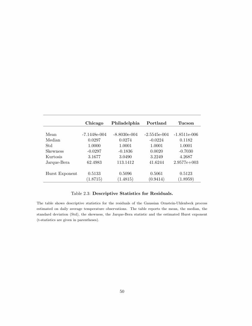
Chicago Philadelphia Portland Tucson

Mean -7.1448e-004 -8.8030e-004 -2.5545e-004 -1.8511e-006Median 0.0297 0.0274 -0.0224 0.1182Std 1.0000 1.0001 1.0001 1.0001Skewness -0.0297 -0.1836 0.0020 -0.7030Kurtosis 3.1677 3.0490 3.2249 4.2687Jarque-Bera 62.4983 113.1412 41.6244 2.9577e+003

Hurst Exponent 0.5133 0.5096 0.5061 0.5123(1.8715) (1.4815) (0.9414) (1.8959)

Table 2.3: Descriptive Statistics for Residuals.

The table shows descriptive statistics for the residuals of the Gaussian Ornstein-Uhlenbeck process

estimated on daily average temperature observations. The table reports the mean, the median, the

standard deviation (Std), the skewness, the Jarque-Bera statistic and the estimated Hurst exponent

(t-statistics are given in parentheses).

50

Panel A: Estimates

N HYP GH NIG

Portlandξ - - 13.4832 -α - 3.8596 5.1992 1.2663β - 0.1290 0.1569 0.1259µ -0.0003 -0.1292 -0.1569 -0.1261δ 1.0001 3.4850 0.0001 3.6681

Tucsonξ - - 0.0134 -α - 2.2873 2.4882 2.0225β - -0.8414 -1.0662 -0.9015µ 0 0.6916 0.8454 0.7311δ 1 0.9843 1.5660 1.4683

Panel B: Tests

N HYP GH NIG

PortlandKolmogorov 1.5058 1.1143 1.0344 5.7808Anderson-Darling 0.0744 0.0350 0.0380 0.0834

TucsonKolmogorov 8.0925 0.6887 1.5221 0.8008Anderson-Darling 0.4296 0.0191 0.0467 0.0225

Table 2.4: Estimated Densities for Residuals.

Panel A reports the estimated parameters of the Normal (N) N(µ, δ), Hyperbolic (HYP) hyp(α, β, δ, µ),

Generalized Hyperbolic (GH) gh(ξ, α, β, δ, µ) and the Normal Inverse Gaussian (NIG) nig(α, β, δ, µ)

distributions fitted to residuals of the Gaussian Ornstein-Uhlenbeck process. The estimates are obtained

by using maximum likelihood approach. Panel B shows the Kolmogorov distances and the Anderson-

Darling statistics, performed to test if the residuals come from the specified distribution . The critical

values of the Kolmogorov test are 1.36 and 1.63 for a confidence level of 5% and 1%, respectively.

The Anderson-Darling statistic presents the disadvantage that it makes use of the specific distribution

in calculating critical values. Currently, tables of critical values are available for normal, lognormal,

exponential, Weibull, extreme value type I, and logistic distributions.

51

Tucson

κ 0.2313 (0.0029)β0 79.4367 (0.5534)β1 15.6006 (0.3570)φ1 4.4312 (0.0221)β2 -1.0331 (0.2262)φ2 8.5869 (0.2260)β3 -0.6979 (0.2063)φ3 2.1081 (0.3100)β4 0.5099 (0.1880)φ4 1.3593 (0.4129)β5 0.4939 (0.1270)φ5 -1.4406 (0.2655)γ0 3.4648 (0.2106)γ1 0.9249 (0.1420)ψ1 -5.3464 (0.0156)γ2 0.2136 (0.0499)ψ2 3.4678 (0.1524)γ3 0.2362 (0.0446)ψ3 -2.9546 (0.0357)α 2.2358 (0.1785)β -0.8319 (0.0560)

Table 2.5: Estimates of the Levy-based Gaussian Ornstein-Uhlenbeck Process.

The table presents the estimates of the unknown parameters of the Levy-based Ornstein-Uhlenbeck

process driving the daily average temperature of Tucson. The estimation approach followed is maximum

likelihood. To measure the significance of parameters the standard errors are reported in parentheses.

52

0 10 20 30 40 50 60 70 80 90 1000

0.002

0.004

0.006

0.008

0.01

0.012

0.014

0.016

0.018

0.02Chicago: Density Estimate of Daily Average Temperature

0 10 20 30 40 50 60 70 80 90 1000

0.002

0.004

0.006

0.008

0.01

0.012

0.014

0.016

0.018

0.02

Philadelphia: Density Estimate of Daily Average Temperature

0 10 20 30 40 50 60 70 80 90 1000

0.005

0.01

0.015

0.02

0.025

0.03

0.035Portland: Density Estimate of Daily Average Temperature

0 10 20 30 40 50 60 70 80 90 1000

0.005

0.01

0.015

0.02

0.025

0.03Tucson: Density Estimate of Daily Average Temperature

Figure 2.1: Estimated Density for Daily Average Temperature.

The figure plots the Gaussian kernel estimates of the density function of daily average temperature.

53

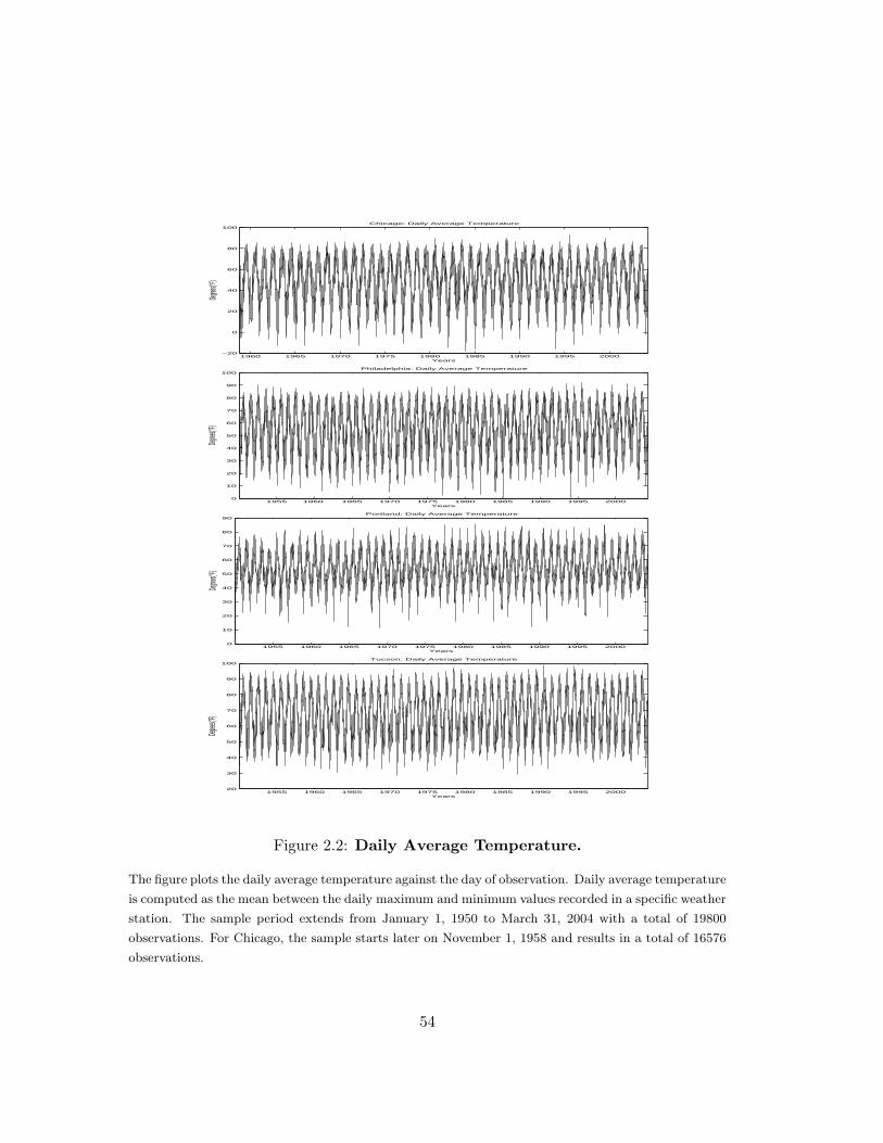
1960 1965 1970 1975 1980 1985 1990 1995 2000−20

0

20

40

60

80

100Chicago: Daily Average Temperature

Years

Degrees

(°F)

1955 1960 1965 1970 1975 1980 1985 1990 1995 20000

10

20

30

40

50

60

70

80

90

100Philadelphia: Daily Average Temperature

Years

Degrees

(°F)

1955 1960 1965 1970 1975 1980 1985 1990 1995 20000

10

20

30

40

50

60

70

80

90Portland: Daily Average Temperature

Years

Degrees

(°F)

1955 1960 1965 1970 1975 1980 1985 1990 1995 200020

30

40

50

60

70

80

90

100Tucson: Daily Average Temperature

Years

Degrees

(°F)

Figure 2.2: Daily Average Temperature.

The figure plots the daily average temperature against the day of observation. Daily average temperature

is computed as the mean between the daily maximum and minimum values recorded in a specific weather

station. The sample period extends from January 1, 1950 to March 31, 2004 with a total of 19800

observations. For Chicago, the sample starts later on November 1, 1958 and results in a total of 16576

observations.

54

Jan Feb Mar Apr May Jun Jul Aug Sep Oct Nov Dec10

20

30

40

50

60

70

80Chicago: Mean

Months

Degrees

(°F)

Jan Feb Mar Apr May Jun Jul Aug Sep Oct Nov Dec20

30

40

50

60

70

80Philadelphia: Mean

Months

Degrees

(°F)

Jan Feb Mar Apr May Jun Jul Aug Sep Oct Nov Dec35

40

45

50

55

60

65

70

75Portland: Mean

Months

Degrees

(°F)

Jan Feb Mar Apr May Jun Jul Aug Sep Oct Nov Dec45

50

55

60

65

70

75

80

85

90Tucson: Mean

Months

Degrees

(°F)

Figure 2.3: Mean of Daily Average Temperature.

The figure plots the mean temperature for each day of the year. The mean is computed as the average

of daily average temperature over many years for each date.

55

Jan Feb Mar Apr May Jun Jul Aug Sep Oct Nov Dec4

6

8

10

12

14

16Chicago: Standard Deviation

Months

Degrees

(°F)

Jan Feb Mar Apr May Jun Jul Aug Sep Oct Nov Dec3

4

5

6

7

8

9

10

11

12Philadelphia: Standard Deviation

Months

Degrees

(°F)

Jan Feb Mar Apr May Jun Jul Aug Sep Oct Nov Dec3

4

5

6

7

8

9

10Portland: Standard Deviation

Months

Degrees

(°F)

Jan Feb Mar Apr May Jun Jul Aug Sep Oct Nov Dec2

3

4

5

6

7

8Tucson: Standard Deviation

Months

Degrees

(°F)

Figure 2.4: Standard Deviation of Daily Average Temperature.

The figure plots the standard deviation for each day of the year. The standard deviation is computed

as the standard deviation of daily average temperature over many years for each date.

56

Jan Feb Mar Apr May Jun Jul Aug Sep Oct Nov Dec−1.5

−1

−0.5

0

0.5

1

1.5Chicago: Skewness

Months

Degrees

(°F)

Jan Feb Mar Apr May Jun Jul Aug Sep Oct Nov Dec−1.5

−1

−0.5

0

0.5

1Philadelphia: Skewness

Months

Degrees

(°F)

Jan Feb Mar Apr May Jun Jul Aug Sep Oct Nov Dec−2

−1.5

−1

−0.5

0

0.5

1

1.5Portland: Skewness

Months

Degrees

(°F)

Jan Feb Mar Apr May Jun Jul Aug Sep Oct Nov Dec−1.5

−1

−0.5

0

0.5

1Tucson: Skewness

Months

Degrees

(°F)

Figure 2.5: Skewness of Daily Average Temperature.

The figure plots the skewness for each day of the year. The skewness is computed as skewness of daily

average temperature over many years for each date.

57

Jan Feb Mar Apr May Jun Jul Aug Sep Oct Nov Dec1.5

2

2.5

3

3.5

4

4.5

5Chicago: Kurtosis

Months

Degrees

(°F)

Jan Feb Mar Apr May Jun Jul Aug Sep Oct Nov Dec1.5

2

2.5

3

3.5

4

4.5

5Philadelphia: Kurtosis

Months

Degrees

(°F)

Jan Feb Mar Apr May Jun Jul Aug Sep Oct Nov Dec1

2

3

4

5

6

7

8

9

10

11Portland: Kurtosis

Months

Degrees

(°F)

Jan Feb Mar Apr May Jun Jul Aug Sep Oct Nov Dec1.5

2

2.5

3

3.5

4

4.5

5

5.5

6Tucson: Kurtosis

Months

Degrees

(°F)

Figure 2.6: Kurtosis of Daily Average Temperature.

The figure plots the kurtosis for each day of the year. The kurtosis is computed as the kurtosis of daily

average temperature over many years for each date.

58

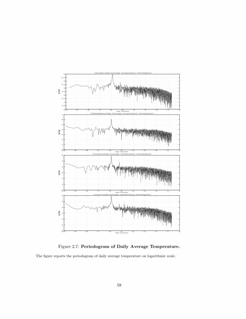
−10 −9 −8 −7 −6 −5 −4 −3 −2 −1 01

1.5

2

2.5

3

3.5

4

4.5

5

5.5

6

log−Cycles

log−Pow

er

Chicago Daily Average Temperature: Periodogram

−10 −9 −8 −7 −6 −5 −4 −3 −2 −1 00

1

2

3

4

5

6

7

log−Cycles

log−Pow

er

Philadelphia Daily Average Temperature: Periodogram

−10 −9 −8 −7 −6 −5 −4 −3 −2 −1 00

1

2

3

4

5

6

log−Cycles

log−Pow

er

Portland Daily Average Temperature: Periodogram

−10 −9 −8 −7 −6 −5 −4 −3 −2 −1 00

1

2

3

4

5

6

log−Cycles

log−Pow

er

Tucson Daily Average Temperature: Periodogram

Figure 2.7: Periodogram of Daily Average Temperature.

The figure reports the periodogram of daily average temperature on logarithmic scale.

59

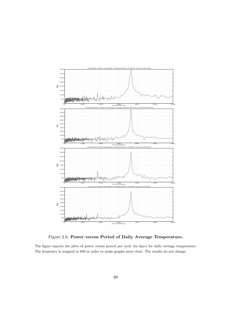
0 100 200 300 400 500 6000

50

100

150

200

250

300

350

400

Period/Days

Power

Chicago Daily Average Temperature: Power versus Period

0 100 200 300 400 500 6000

50

100

150

200

250

300

350

400

450

Period/Days

Power

Philadelphia Daily Average Temperature: Power versus Period

0 100 200 300 400 500 6000

50

100

150

200

250

300

350

400

Period/Days

Power

Portland Daily Average Temperature: Power versus Period

0 100 200 300 400 500 6000

50

100

150

200

250

300

350

400

450

Period/Days

Power

Tucson Daily Average Temperature: Power versus Period

Figure 2.8: Power versus Period of Daily Average Temperature.

The figure reports the plots of power versus period per cycle (in days) for daily average temperature.

The frequency is stopped to 600 in order to make graphs more clear. The results do not change.

60

−10 −9 −8 −7 −6 −5 −4 −3 −2 −1 03

4

5

6

7

8

9

log−Cycles

log−Pow

er

Chicago Temperature Variance: Periodogram

−10 −9 −8 −7 −6 −5 −4 −3 −2 −1 03

4

5

6

7

8

9

log−Cycles

log−Pow

er

Philadelphia Temperature Variance: Periodogram

−10 −9 −8 −7 −6 −5 −4 −3 −2 −1 02

3

4

5

6

7

8

9

log−Cycles

log−Pow

er

Portland Temperature Variance: Periodogram

−10 −9 −8 −7 −6 −5 −4 −3 −2 −1 03

4

5

6

7

8

9

log−Cycles

log−Pow

er

Tucson Temperature Variance: Periodogram

Figure 2.9: Periodogram of Variance of Daily Average Temperature.

The figure reports the periodogram of variance of daily average temperature on logarithmic scale. The

squared daily average temperature is used as proxy for variance.

61

0 100 200 300 400 500 6000

500

1000

1500

2000

2500

3000

3500

4000

Period/Days

Power

Chicago Temperature Variance: Power versus Period

0 100 200 300 400 500 6000

500

1000

1500

2000

2500

3000

3500

4000

4500

5000

Period/Days

Power

Philadelphia Temperature Variance: Power versus Period

0 100 200 300 400 500 6000

500

1000

1500

2000

2500

3000

3500

4000

Period/Days

Power

Portland Temperature Variance: Power versus Period

0 100 200 300 400 500 6000

500

1000

1500

2000

2500

3000

3500

4000

4500

5000

Period/Days

Power

Tucson Temperature Variance: Power versus Period

Figure 2.10: Power versus Period of Variance of Daily Average TemperatureVariance.

The figure reports the plots of power versus period per cycle (in days) of variance of daily average

temperature. The squared daily average temperature is used as a proxy for variance. The frequency is

stopped to 600 in order to make graphs more clear. The results do not change.

62

−30 −20 −10 0 10 20 300

500

1000

1500

2000

2500

3000

3500Chicago: Daily Average Temperature First Difference

−30 −20 −10 0 10 20 300

500

1000

1500

2000

2500

3000

3500

4000

4500Philadelphia: Daily Average Temperature First Difference

−20 −15 −10 −5 0 5 10 150

500

1000

1500

2000

2500

3000

3500

4000

4500Portland: Daily Average Temperature First Difference

−25 −20 −15 −10 −5 0 5 10 15 200

500

1000

1500

2000

2500

3000

3500

4000

4500

5000Tucson: Daily Average Temperature First Difference

Figure 2.11: Histogram of First Difference of Daily Average Temperature.

The figure plots the histogram of the first difference of daily average temperature. The solid line draws

the density curve of a theoretical normal random variable with mean and standard deviation evaluated

from the observed time series.

63

0 2000 4000 6000 8000 10000 12000 14000 16000−4

−3

−2

−1

0

1

2

3

4Chicago Temperature Anomalies

0 2000 4000 6000 8000 10000 12000 14000 16000 18000−5

−4

−3

−2

−1

0

1

2

3

4Philadelphia Temperature Anomalies

0 2000 4000 6000 8000 10000 12000 14000 16000 18000−5

−4

−3

−2

−1

0

1

2

3

4Portland Temperature Anomalies

0 2000 4000 6000 8000 10000 12000 14000 16000 18000−6

−5

−4

−3

−2

−1

0

1

2

3

4Tucson Temperature Anomalies

Figure 2.12: Residuals.

The figure plots the estimated residuals, obtained by fitting the Ornstein-Uhlenbeck process to historical

observations of daily average temperature using maximum likelihood method.

64

0 2 4 6 8 10 12 14 16 18 20−0.2

−0.15

−0.1

−0.05

0

0.05

0.1

0.15Chicago: Sample autocorrelation coefficients

k−values

sacf va

lues

0 2 4 6 8 10 12 14 16 18 20−0.2

−0.15

−0.1

−0.05

0

0.05

0.1

0.15Philadelphia: Sample autocorrelation coefficients

k−values

sacf va

lues

0 2 4 6 8 10 12 14 16 18 20−0.08

−0.06

−0.04

−0.02

0

0.02

0.04

0.06

0.08

0.1Portland: Sample autocorrelation coefficients

k−values

sacf va

lues

0 2 4 6 8 10 12 14 16 18 20−0.15

−0.1

−0.05

0

0.05

0.1

0.15

0.2Tucson: Sample autocorrelation coefficients

k−values

sacf va

lues

Figure 2.13: Autocorrelation Coefficients of Residuals.

The figure displays the empirical autocorrelation function for estimated residuals. The dot line designs

the estimated 95% confidence interval.

65

−10 −9 −8 −7 −6 −5 −4 −3 −2 −1 00

0.5

1

1.5

2

2.5

3

3.5

log−Cycles

log−Pow

er

Chicago Temperature Anomalies: Periodogram

−10 −9 −8 −7 −6 −5 −4 −3 −2 −1 00

0.5

1

1.5

2

2.5

3

3.5

log−Cycles

log−Pow

er

Philadelphia Temperature Anomalies: Periodogram

−10 −9 −8 −7 −6 −5 −4 −3 −2 −1 00

0.5

1

1.5

2

2.5

3

3.5

log−Cycles

log−Pow

er

Portland Temperature Anomalies: Periodogram

−10 −9 −8 −7 −6 −5 −4 −3 −2 −1 0−0.5

0

0.5

1

1.5

2

2.5

3

3.5

log−Cycles

log−Pow

er

Tucson Temperature Anomalies: Periodogram

Figure 2.14: Periodogram of Residuals.

The figure reports the periodogram of estimated residuals on logarithmic scale.

66

−10 −9 −8 −7 −6 −5 −4 −3 −2 −1 00

0.5

1

1.5

2

2.5

3

3.5

log−Cycles

log−Pow

er

Chicago Temperature Anomalies Variance: Periodogram

−10 −9 −8 −7 −6 −5 −4 −3 −2 −1 00.5

1

1.5

2

2.5

3

3.5

log−Cycles

log−Pow

er

Philadelphia Temperature Anomalies Variance: Periodogram

−10 −9 −8 −7 −6 −5 −4 −3 −2 −1 0−0.5

0

0.5

1

1.5

2

2.5

3

3.5

log−Cycles

log−Pow

er

Portland Temperature Anomalies Variance: Periodogram

−10 −9 −8 −7 −6 −5 −4 −3 −2 −1 00

0.5

1

1.5

2

2.5

3

3.5

log−Cycles

log−Pow

er

Tucson Temperature Anomalies Variance: Periodogram

Figure 2.15: Periodogram of Variance of Residuals.

The figure reports the periodogram of the variance of estimated residuals on logarithmic scale. The

square of residuals is used as proxy for variance.

67

−5 −4 −3 −2 −1 0 1 2 3 4 5−4

−3

−2

−1

0

1

2

3

4

Standard Normal Quantiles

Quantile

s of Re

siduals

Chicago: QQ Plot of Residuals versus Standard Normal

−5 −4 −3 −2 −1 0 1 2 3 4 5−5

−4

−3

−2

−1

0

1

2

3

4

5

Standard Normal Quantiles

Quantile

s of Re

siduals

Philadelphia: QQ Plot of Residuals versus Standard Normal

−5 −4 −3 −2 −1 0 1 2 3 4 5−5

−4

−3

−2

−1

0

1

2

3

4

Standard Normal Quantiles

Quantile

s of Re

siduals

Portland: QQ Plot of Residuals versus Standard Normal

−5 −4 −3 −2 −1 0 1 2 3 4 5−6

−5

−4

−3

−2

−1

0

1

2

3

4

Standard Normal Quantiles

Quantile

s of Re

siduals

Tucson: QQ Plot of Residuals versus Standard Normal

Figure 2.16: QQ-Plot of Residuals.

The figure displays a quantile-quantile plot of the quantile of estimated residuals versus theoretical

quantiles from a normal distribution.

68

−5 −4 −3 −2 −1 0 1 2 3 4 50

0.1

0.2

0.3

0.4

0.5

x

Pro

ba

bility

Portland: Emprical and Fitted Densities for Residuals

NormalHyperbolicEmpiricalGeneralized Hyperbolic

−5 −4 −3 −2 −1 0 1 2 3 4 5−14

−12

−10

−8

−6

−4

−2

0

x

log

−P

ro

ba

bility

Portland: Emprical and Fitted Densities for Residuals on a logarithmic scale

NormalHyperbolicEmpiricalGeneralized Hyperbolic

Figure 2.17: Empirical and Fitted Densities for Residuals of Portland.

The figure reports the empirical densities together with the fitted Normal, Hyperbolic and Generalized

Hyperbolic distributions on the original and logarithmic scales for estimated residuals of Portland. The

empirical density is estimated by using a Gaussian kernel smoother.

69

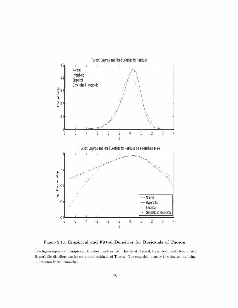
−6 −5 −4 −3 −2 −1 0 1 2 3 40

0.1

0.2

0.3

0.4

0.5

x

Pro

ba

bility

Tucson: Emprical and Fitted Densities for Residuals

NormalHyperbolicEmpiricalGeneralized Hyperbolic

−6 −5 −4 −3 −2 −1 0 1 2 3 4−20

−15

−10

−5

0

x

log

−P

ro

ba

bility

Tucson: Emprical and Fitted Densities for Residuals on a logarithmic scale

NormalHyperbolicEmpiricalGeneralized Hyperbolic

Figure 2.18: Empirical and Fitted Densities for Residuals of Tucson.

The figure reports the empirical densities together with the fitted Normal, Hyperbolic and Generalized

Hyperbolic distributions for estimated residuals of Tucson. The empirical density is estimated by using

a Gaussian kernel smoother.

70

Chapter 3

Pricing Weather Derivatives

This Chapter is devoted to derive formulas to price futures contracts based on US tem-

perature indexes. Weather derivatives market is a typical example of so-called incom-

plete markets in terms of the underlying asset, i.e. temperature, which is not tradable.

Even more, including Levy processes in the model for spot dynamics of Tucson leads

to even higher degree of incompleteness. In such markets a continuum of arbitrage-free

prices exists, one for each equivalent martingale measure. All equivalent probability

measures are also martingale measures, since there is not basic security, such as a stock

or a treasury bond whose price is uniquely related to the temperature index.

To price derivatives written on temperature, it is necessary to take into account the

risk preferences of investors. Traditionally these are described by the market price of risk

charged for issuing the derivatives. The risk premium represents an additional unknown

parameter in the model, coming from the equivalent martingale measure. I will derive

these martingale measures through the Girsanov theorem for the model with standard

Brownian motion as driving noise and through the Esscher transform for the Levy-based

Ornstein-Uhlenbeck model. At the end of this Chapter I will provide an estimate of the

implicit risk premium by calibrating the theoretical model to the observed prices. The

71

present thesis considers a time-dependent parametrization of the market price of risk,

in order to produce a more flexible class of martingale measures. The statistical and

dynamics properties of the implicit risk premium will be also studied.

3.1 Temperature-Based Futures Contracts

US Weather futures contracts are based on the CME (Chicago Mercantile Exchange)

degree days indexes, which represents the cumulative sum of daily CDDs or HDDs over

a calendar month or a season. In particular, here I concentrate my considerations on

the pricing of futures written on monthly cumulative degree day indexes.

Let be t1 and tn the first and the last calendar day of the contract month respectively.

Hence, the cumulative CDDn degree day index is computed as:

CDDn =n∑

i=1

max {T (ti)− 65, 0} (3.1)

and the HDDn degree day index is:

HDDn =n∑

i=1

max {65− T (ti), 0} (3.2)

Note that for both CDD and HDD derivatives the value is highly non-linear with respect

to the daily average temperature, property which bears a number of consequences.

Futures contracts are cash-settled, which means that there is a daily marking to

market based upon the index, with the gain or loss applied to the customer’s account.

At the end of the period, the underlying, i.e. temperature, cannot be delivered and

outstanding contracts are closed by cash settlement.

Several authors have studied the problem of pricing derivatives on temperature. In

Alaton, Djehiche, and Stillberger (2002) the fair value of an option written on HDD

index over a month is derived using an approximation formula as well as Monte Carlo

simulations. Brody, Syroka, and Zervos (2002) find the price of different temperature

72

options based on fractional Brownian dynamics as solution of partial differential equa-

tions. They calculate the price at the time when the contract is entered. Later on,

Benth (2003) generalizes the work of Brody, Syroka, and Zervos (2002) by deriving the

time dynamics of temperature options. Furthermore, Benth and Saltyte-Benth (2005a)

derive the price dynamics of futures written on cumulative average temperature (CAT)

over a season. Unlike previous literature, Benth and Saltyte-Benth (2005a) abandon the

normality assumption and introduce the Levy motion in the temperature time evolution.

The weather market is a typical example of so-called incomplete markets, since the

underlying weather factor cannot be used for trading purposes. Even more, introducing

Levy processes as the driving noise in the spot dynamics leads to even higher degree

of incompleteness. As a consequence, an infinite number of admissible risk-neutral

probabilities exists and the no arbitrage argument alone is not sufficient to determine

unique prices. The usual technique in commodity and interest-rate markets to single

out one martingale measure Q consists in paremetrizing the class of Q’s by the market

price of risk parameter and in fitting theoretical prices to the empirical ones. So doing,

I will pick up the equivalent martingale measure “chosen by the market”. Once the risk

neutral spot dynamics is determined, computing futures prices is a fairly straightforward

exercise.

Assuming a constant continuously compounding interest rate r, the futures price

at time ts < t1 written on the cumulated degree day index Hn (CDDn or HDDn) is

defined as the F(ts)-adapted stochastic process FHn(ts) satisfying:

0 = e−r(tn−ts)EQ [Hn− FHn(ts) | F(ts)] (3.3)

with Q the martingale measure. From the adaptedness of FHn(ts), I easily find the

futures price to be:

FHn(ts) = EQ [Hn | F(ts)] (3.4)

73

Formula (3.4) remarks that it is necessary to determine the equivalent martingale

measures Q in order to determine futures prices. To this end, I apply the Girsanov

theorem for the models with standard Brownian motion as driving noise and the Esscher

transform for the Levy-based Ornstein-Uhlenbeck process.

3.2 Pricing Under The Assumption of Brownian Motion

As Driving Noise

It is known from the Girsanov theorem that the change-of-measure of Brownian pro-

cesses corresponds to a shift of the drift of the underlying process by the price of risk,

here denoted by λ(t). By looking to the SDE (2.8), the spot dynamics under the mar-

tingale measure Q (characterized by the market price of risk λ(t)) is:

dT (t) ={

dθ(t)dt

+ κ [θ(t)− T (t)]− λ(t)σ(t)}

dt + σ(t)dV (t) (3.5)

with V (t) being the Q-Brownian process. Note that I adopt a time-dependent param-

eterization of the market price of risk λ(t), in order to produce a more flexible class

of martingale measure Q. Since the price of a futures contract is expressed as the

expected value (3.4) under the martingale measure Q, I need to known explicitly the

distributional properties of daily temperature T (t) under the martingale measure Q.

As exposed in section 2.2.1, daily temperature T (t) (given F(ts)) follows a Gaussian

distribution. Given that the Girsanov transformation only changes the drift term, T (t)

has still a Gaussian distribution under the measure Q. Now I need to compute the

expected value and the variance of T(t) under Q. From (3.5) it follows that:

µ(t) = EQ [T (t)|F(s)] = EP [T (t)|F(s)]−∫ t

sλ(u) σ(u) e−κ(t−u) du (3.6)

74

where the conditional expected value under the objective measure P is given by the

equation (2.11). Indeed, the variance v2(t) is the same under both measures P and Q

and it is given by integral (2.12).

Concluding, under the martingale measure Q and given information at time s < t,

T (t) is a Gaussian variable:

Tt∼N(µ(t), v2(t))

where µ(t) is given by (3.6) and v(t)2 by (2.12).

The contracts (3.1) and (3.2) are a type of Asian options, since the payout depends

on the accumulation of the degree day indexes over the contract month. In such a case,

the out-of-period price (period of accumulation) is uniquely determined by the model

forecasts, while the in-period expectations are adjusted by the observed temperatures.

For this reason, I consider the out-of-period and the in-period pricing separately in the

following subsections.

3.2.1 Out-of-Period Valuation

Let be t1 and tn the first and the last calendar day of the contract month respectively.

The formula to pricing a CDDn future contract at time ts < t1 is:

FCDDn(ts) = EQ[

n∑

i=1

max{T (ti)− 65, 0} | F(ts)

]

=n∑

i=1

EQ [max{T (ti)− 65, 0} | F(ts)]

=n∑

i=1

[∫ ∞

65(x− 65) fQT (ti)

(x) dx

]

=n∑

i=1

[(µ(i)− 65)Φ(−α(i)) +

v(i)√2π

e−α(i)2

2

](3.7)

75

where α(i) = (65− µ(i))/v(i) and Φ denotes the cumulative distribution function for a

standard normal distribution. µ(i) and v(i) represent the first and second conditional

moment of temperature given information at time ts. Appendix A.1 explicitly reports

the derivation of formula (3.7).

In the same way the price of an HDDn future contract at time ts < t1 is computed

as:

FHDDn(ts) = EQ[

n∑

i=1

max {65− T (ti), 0} | F(ts)

]

=n∑

i=1

EQ [max {65− T (ti), 0} | F(ts)]

=n∑

i=1

[∫ 65

0(65− x) fQT (ti)

(x) dx

]

=n∑

i=1

[(65− µ(i))

(Φ (α(i))− Φ

(−µ(i)

v(i)

))

+v(i)√

2π

(e−

α(i)2

2 − e− 1

2

�µ(i)v(i)

�2)]

(3.8)

Note that the fair value of a weather derivative at time ts < t1 is uniquely based on

temperature forecasting.

3.2.2 In-Period Valuation

In order to evaluate the futures price inside the contract period t1≤tj≤tn, the formulas

presented above must be modified. The reason is that the out-of-period valuation is

only based on the model forecasts, while at tj I know temperatures recorded between

76

t1 and tj . To this end, I split the formulas (3.7) and (3.8). For instance, the price of a

CDDn futures contract at time t1≤tj≤tn is determined as follows:

FCDDn(tj) = EQ[

n∑

i=1

max {T (ti)− 65, 0} | F(tj)

]

=n∑

i=1

EQ [max {T (ti)− 65, 0} | F(tj)]

=j∑

i=1

max {T (ti)− 65, 0}+n∑

m=j+1

EQ [max {T (tm)− 65, 0} | F(tj)]

(3.9)

Note that the price is given by the sum of two distinct terms. The first term is known

at tj , while the second one is stochastic. Suppose that tj is today. At that time I know

the daily temperature recorded from the beginning of the contract period t1 to today

tj , but not which one will verify from tomorrow tj+1 until the end of the month tn. In

the same way the formula for pricing HDDn contracts (3.8) can be modified.

3.3 Pricing Under The Assumption of Levy Motion As

Driving Noise

The inclusion of a Levy process (L(t))t≥0 with infinitely divisible hyperbolic law adds

up the complexity in evaluating derivatives. The problem arises from the fact that

hyperbolic distributions are not closed under convolution1, in the sense that they do

not provide an exact expression for the density of L(t), for t 6= 1. The Fourier transform

1The normal inverse Gaussian distribution is the only sub-class of generalized hyperbolic laws whichsatisfies the following convolution property:

NIGt(α, β, δ, µ) = NIG(α, β, tδ, tµ)

with the mean and variance of independent random variables summing up.

77

approach can be applied to address this problem. Following this important theorem, the

unknown density fX is obtained by the Fourier inversion integral of the corresponding

characteristic function ψX :

fX(x) =12π

∫ +∞

−∞e−isxψX(s)ds (3.10)

As documented in previous section, the fair value of a futures contract written on

CDDn at ts < t1 (out-of-period) can be expressed as:

FCDDn(ts) = EQ[

n∑

i=1

max{T (ti)− 65, 0} | F(ts)

]

=n∑

i=1

EQ [max{T (ti)− 65, 0} | F(ts)]

=n∑

i=1

∫ ∞

65(x− 65)fQT (ti)

(x)dx (3.11)

with fQT (ti)(x) denoting the Esscher risk-neutral density function of T (ti) conditional on

F(ts). The Esscher transform is reported in appendix A.2. Note that Q is the same

martingale measure of section 3.2, fixed by the market price of risk λ(t). By the same

way the formula for HDDn futures price can be written as:

FHDDn(ts) =n∑

i=1

∫ 65

0(65− x)fQT (ti)

(x)dx (3.12)

Formulas (3.11) and (3.12) put in evidence that it is necessary to know the density

function fQT (ti)in order to evaluate futures contracts. As mentioned above, it is not

possible to derive the analytic formula of fQT (ti)starting from the assumption that L(1)

is hyperbolic distributed, because the convolution property does not hold. However,

formula (3.10) reveals that knowing the characteristic function ψQT paves the way for a

Fourier approach to compute fQT (ti).

78

Following Benth and Saltyte-Benth (2004)[corollary 4.4], I derive that the charac-

teristic function ot T (ti) under the martingale measure Q is given by:

ψQT = EQ [exp{imT (ti)} | F(ts)] = exp{Ψ(m)} (3.13)

where:

Ψ(m) = im[T (ts)− θ(ts)]e−κ(ti−ts) + imθ(ti)−∫ ti

ts

φ(λ(u))du

+∫ ti

ts

φ(ime−κ(ti−u)σ(u) + λ(u)

)du (3.14)

with m ∈ R and φ(·) being the moment generating function of L(1) and i =√−1. The

proof is exposed in appendix A.2. Hence, the distributional properties of T (ti) can be

obtained by numerical inversion of the corresponding characteristic function ψQT as in

integral (3.10). I refer to Carr and Madan (1999) for a complete description of the Fast

Fourier algorithm for calculating the integral (3.10).

Note that this section focuses on the out-of-period valuation of derivatives. For in-

period pricing, expectations in (3.11) and (3.12) are splitted in two terms, as exposed

in section 3.2.2.

The derivation of pricing formulas of futures contracts written on CDD and HDD in-

dexes when the Levy motion is the driving noise of temperature dynamics represents one

of the important contributions of this thesis. As far as I know, only Benth and Saltyte-

Benth (2005a) apply Levy processes in modelling weather derivatives. The stochastic

process of daily temperature, measured at Tucson, is very similar to the model specified

in Benth and Saltyte-Benth (2005a). However, important differences distinguish these

two works. First, in this thesis I propose to use Levy process with marginal following

the sub-class of hyperbolic distribution instead of the generalized hyperbolic family ap-

plied in Benth and Saltyte-Benth (2005a). As documented in section 2.3, this choice is

79

determined by the time series analysis of historical data and it offers the advantage to

reduce the time of estimation. Still, there is another important difference concerning

the pricing. Benth and Saltyte-Benth (2005a) concentrate their considerations on the

pricing of futures written on Cumulative Average Temperature (CAT) for European

cities, instead of contracts based on the cumulated US degree-day indexes. The CAT

structure is less complex than cumulated degree-day indexes. In fact, it is simply defined

as the sum of temperatures over the accumulation period:

CAT =n∑

i=1

T (ti) (3.15)

with t1 and tn the first and last calendar day of the contract period. The simple

construction of (3.15) index allows to obtain analytic formulas for pricing when the

Levy process is assumed as driving noise. This is not my case, where expression (3.11)

and (3.12) can only be evaluated numerically.

Given the complexity of formulas (3.11) and (3.12), I proceed as follows. I fix the

unknown parameter λ(t) by calibrating the theoretical prices to the observed ones only

by using data for Chicago, Philadelphia, Portland. As exposed above, these cities admit

explicit formulas for pricing future contracts, since their temperature anomalies satisfy

the normality hypothesis. Then the integrals in (3.11) and (3.12) for the city of Tucson

can be evaluated by using the estimate λ(t) in the Fast Fourier approach.

3.4 Calibrating the Model to the Market

In this section I proceed to single-out a martingale measure Q by calibrating the the-

oretical model to historical data. Indeed, I estimate the implicit market price of risk

λ(t) by comparing theoretical futures prices, given in previous formulas, to the prices

observed in the market.

80

The estimate of the market price of risk represents another important contribution

of this research. As far as I known, only Alaton, Djehiche, and Stillberger (2002) provide

an estimate of the market price of risk for weather market by calibrating the model to

Swedish market options. However, their result is only indicative, because the prices

used are not market quoted, but offered by Scandic Energy Company and only refer

to two HDD options. Even more, they provide explicit formulas to pricing options by

making the strong assumption that temperature is extremely small than the base level

on the winter period of HDD contracts.

The dataset used for calibration purposes includes all futures prices on CDD and

HDD indexes available for Chicago, Philadelphia and Portland. More precisely, the

sample collects futures contracts with contract period which extends from January 2002

to February 2004.

Several minimizing criterion functions are implemented in this thesis. First, the

objective function is defined as the sum of squared distance between the observed futures

price for a particular day Pit and the corresponding theoretical price P ∗it. Specifically,

for each day t I solve the problem:

minN∑

i=1

(Pit − P ∗it)

2 (3.16)

where the sum is taken over all N futures contracts available at day t. Given that

the weather derivatives market is still not liquid as traditional financial markets, I also

adopt the weighted sum of squared distance as objective function:

minN∑

i=1

wi,t(Pit − P ∗it)

2 (3.17)

with wi,t denoting the trading volume of contract i for the trading day t. Finally, I

repeat the minimization problem by considering only price changes due to corresponding

volume changes. In this case, I set the variable wit in (3.17) to be a dummy variable

81

which assumes value one if the volume for contract i on trading day t is non null,

otherwise it is equal to zero.

First I provide an estimate of the market price of risk by assuming that this quantity

is constant over time. Table 3.1 Panel A reports the non linear least square (LS), the

weighted non linear least square (LS-WEIGHTED) and the non linear least square

estimate obtained by considering uniquely trading days with non-zero trading volume

(LS-VOLUME). The parameter estimates are given for three different samples of data:

first by using prices on CDD and HDD contracts separately, then by collecting all

prices (CDD&HDD) futures contracts. In all cases λ(t) has a negative sign. For the

LS-VOLUME estimate I report the standard deviation in parenthesis, estimated via

Monte Carlo simulations. The calculation consists of 500 simulation runs2. From the

estimated standard deviation it is clear that the zero risk premium hypothesis is rejected.

This result provides evidence in support to the study of Cao and Wei (2004). These

authors show that the market price of risk associated with the temperature variable is

significant by extending the Lucas (1978)’ equilibrium asset-pricing model. The risk

premium charged for the CDD futures is more closed to zero than the one for HDD

contracts for all estimations. This result indicates that the CDD and HDD contracts

are not priced using the same market price of risk. Thus it can be concluded that the

assumption of a constant market price of risk is violated.

Figure 3.1 presents the estimated temperature risk premium for each trading day t

based on a weighted non linear least square estimation procedure on the complete set of

futures contracts. The estimate varies from −2.8899 to 1.1985. Two remarkable nega-

tive peaks take place on 31 December 2002 and 31 December 2003. Unfortunately I am

not able to interpret these results. Table 3.1 Panel B gives the mean value (−0.0799) and

the standard deviation (0.2410) of the daily market price of risk. In order to better un-

2I do not report the estimated standard deviation for each estimate because the computational costsare too high.

82

derstand the tendency of the risk premium, I report in Figure 3.2 the smoothed series. I

observe that the market price of risk stretches to increase and to become positive during

the warmer months (from May to August), that is when CDD contracts are traded. The

opposite behaviour verifies during the winter period when HDD contracts are traded,

with the exception of a positive peak at the end of December 2002. This result is consis-

tent with Cao and Wei (2004)’s finding that the correlation between consumption and

temperature show a seasonal pattern. The reason is that the higher/lower temperatures

in summer/winter months are associated with more consumption for energy and power

products. The rank of variation of the implicit market price of risk seems to increase

with passing of time. Probably this is explained by the increment of the exchanges in

the market. Moreover, the estimate reveals the widest distance from the null value in

correspondence of the months with extreme temperatures, that is the warmer (July and

August) and the colder (January and February) months. This means that the futures

contracts on months with extreme temperatures are charged by a greater premium.

A positive (negative) estimate of the market price of risk implies that the underlying

process (3.5) under the fixed Q coincides with the one written on the same underlying in

a risk neutral world in equation (2.8), but with a lower (higher) temperature expected

drift. A smaller (greater) temperature drift has different consequences on CDD contracts

with respect to HDD contracts, because of the dissimilarity in the degree day index

construction. To understand the meaning of the sign of the parameter, I focus on

the relationship between the futures prices and the expected value of the “underlying

asset”. From Figure 3.2 I get that the positive (negative) sign prevails for CDD (HDD)

contracts. For a CDD futures contract a positive risk premium implies that the futures

price is below the expected futures spot price. The same relation between futures price

and expected spot price holds true for HDD contracts in presence of a negative risk

premium. Because the futures price and the spot price must be equal at maturity, this

implies that the futures price should, on average, increase over the life of the contract. In

83

this situation, speculators tend to hold long positions to make profits and hedgers tend

to hold short positions. The reason is that to compensate the speculators for the risk

they are bearing, there must be an expectation that the futures price will rise over time.

On the other hand, hedgers decide to enter into contracts even in presence of negative

expected payoffs, because they are reducing their risks and this hedging instrument is

less expensive than insurance contracts. This result provides evidence in support to the

“Normal Backwardation” theory, argued by Keynes (1930). For instance, an heating oil

retailer may feel that if the winter is very cold it will have high revenues, so it might sell

a HDD futures contract. If the winter is not particularly cold, it receives compensation

from the futures contract. On the other hand, if the winter is very cold, the retailer can

afford to finance the payout of the futures, because its revenues are high. In a similar

way, an energy company might decide to sell a CDD futures contracts to reduce its risk

exposure during the warm season.

3.4.1 Analysis of the Daily Market Price of Risk

Figures 3.1 and 3.2 show that the market price of risk is time-varying and probably

related to the nature of the traded contracts. Here I try to determine how the market

price of risk evolves. Understanding which factors affect the risk premium may still

improve pricing. Clearly variables like the lag of the market price of risk λ(t − 1) and

the number of contracts available for trading on the market η(t) may be useful to predict

the market price of risk at day t. A simple regression:

λ(t) = β0 + β1λ(t− 1) + β2η(t) + ε(t) (3.18)

is estimated. The estimates and their t-statistics (in parenthesis) are reported in Table

3.2. All the variables enter with a significant value in the regression. There is a positive

relationship between the risk premium and its lag. The variable η(t) has a positive

impact on λ(t). This might be explained by the extra diversification possibilities that

84

exist when more contracts are available for trading. In fact, if more futures contracts

are available for trading, the risk premium is closer to 0, given that λ(t) is on average

negative.

It could be interesting to study the seasonality effects of the risk premium. To this

end, I repeat the estimation of eq.(3.18) by introducing two dummy variables:

λ(t) = β0 + β1λ(t− 1) + β2η(t) + β3DCDD(t) + β4DHDD(t) + ε(t) (3.19)

where DCDD assumes value 1 from May to September otherwise 0; while DHDD assumes

value 1 from November to March otherwise 0. Note that I do not consider the so-

called shoulder months (April and October), in order to make the difference between

seasons more remarkable. Table 3.2 reports the results. The dummy variables exhibit

parameters non statistically significant. Probably it is necessary to have more data for

being able to carry out the analysis of the seasonality oscillations. The dummy variable

DCDD(t) enters with a positive value. This implies that the risk premium increases

(given that it is negative in mean) and it can also become positive during the warmest

months. The negative sign of DHDD(t) indicates that the more the temperatures are

low the more is negative the sign of the parameter. These findings seem to be in tuning

with the interpretation of Figure 3.2 exposed above.

85

Panel A: Constant Market Price of Risk

LS LS-WEIGHTED LS-VOLUME

CDD -0.0587 -0.0331 -0.0399HDD -0.1456 -0.1018 -0.0942CDD & HDD -0.1114 -0.0590 -0.0650

(0.0066)

Panel B: Time-varying Market Price of Risk

LS LS-WEIGHTED LS-VOLUME

mean -0.0779std 0.2410

Table 3.1: Estimate of the Market Price of Risk .

Panel A reports the non linear least square (LS), the weighted non linear least square (LS-WEIGHTED)

and non linear least square estimate obtained by considering uniquely trading days with non-zero trading

volume (LS-VOLUME). The parameter estimates are given for three different samples of data: first by

using prices on CDD and HDD contracts separately, then by collecting all prices (CDD&HDD) futures

contracts. The dataset used includes all futures prices on CDD and HDD indexes available for Chicago,

Philadelphia and Portland. More precisely, the sample collects futures contracts with contract period

which extends from January 2002 to February 2004. For the LS-VOLUME estimate, the estimated

standard deviation is reported in parenthesis. Panel B gives the mean and the standard deviation (Std)

of the daily market price of risk. This time-varying estimate is based on a weighed non linear least

square estimation procedure on the complete set of futures prices.

86

Risk Premium Analysisc -0.1459 -0.1331

(-4.8513) (-3.2232)λ(t− 1) 0.1403 0.1310

(3.4524) (3.1899)η(t) 0.0029 0.0020

(2.8272) (1.8094)DCDD - 0.0307

- (0.9630)DHDD - -0.0218

- (-0.6394)

R2 0.0369 0.0452

Table 3.2: Estimates of the Market Price Analysis Regression.

This table reports the OLS estimates of the regression of the market price of risk λ(t) on the following

regressors: its first lag λ(t − 1) and the number of contracts available for trading η(t), the dummy

variable for warm months DCDD and the dummy variable for cold months DHDD. The t-statistics are

given in parenthesis. R2 represents the coefficient of determination of the regression.

87

Jan02 May02 Sep02 Jan03 May03 Sep03 Jan04−3

−2.5

−2

−1.5

−1

−0.5

0

0.5

1

1.5Daily Market Price of Risk

Figure 3.1: Daily Market Price of Risk.

The figure reports the daily market price of risk estimated by calibrating the model to the observed

market prices. The estimate is obtained by applying the non linear weighted square estimation procedure

on the complete set of futures contracts in the sample.

Jan02 May02 Sep02 Jan03 May03 Sep03 Jan04−0.8

−0.6

−0.4

−0.2

0

0.2

0.4

0.6Smoothed Market Price of Risk

Figure 3.2: Smoothed Market Price of Risk.

The figure reports the smoothed market price of risk at daily frequency. The smoothed series is computed

by applying the exponential smoothing method.

88

Conclusions

Weather derivatives have gained popularity in financial markets as a tool to hedge

weather risk. Markets for weather related products are emerging (e.g. Chicago Mer-

cantile Exchange) and this remarks the necessity for dynamical models of derivatives

in order to understand their risk exposure. From the point of view of modern finance

theory, weather derivatives market is hardly at a desirable stage and the market itself is

expected to evolve further. This thesis has addressed issues pertaining the development

of a good model for temperature and pricing weather derivatives.

In the present dissertation I have analyzed temperature data measured on four US

stations: Chicago, Philadelphia, Portland and Tucson. On the basis of statistical prop-

erties of historical data, I have proposed a Gaussian Ornstein-Uhlenbeck model with

time-dependent mean and volatility to describe the stochastic dynamics of tempera-

ture. I include truncated Fourier series to capture seasonality in the mean and volatil-

ity. Importantly, seasonal fluctuations differ noticeably across cities both in terms of

amplitude and frequency. My simple model is sophisticated enough to incorporate the

basic stylized facts of temperature data with the only exception of the city of Tucson.

In such a case the unequivocal evidence of fat tails and negative skewness in the distri-

bution of standardized residuals have suggested the exploration of different alternatives.

I have modelled this by substituting standard Brownian motion with Levy process. In

particular, temperatures recorded at Tucson reveal that the hyperbolic class fit very

89

well the empirical distribution. In contrast with previous studies, I have found that

the standardized residuals have not fractional characteristics after having removed all

seasonal cycles present in data.

Regarding the pricing, I have provided formulas for futures contracts on US cu-

mulated degree day indexes. I have calculated explicit arbitrage-free prices using the

Gaussian Ornstein-Uhlenbeck model. However, introducing Levy process in the tem-

perature dynamics precludes the possibility to find explicit formulas. This case must

be solved numerically and I have derived the characteristic function under the risk-

neutral probability measure, a key ingredient in the Fourier inversion approach to find

the density function used for pricing.

Finally, futures prices are generated by the market price of risk, since the weather

derivatives market is a typical example of incomplete market. I have estimated this

parameter by calibrating theoretical prices to the actual quoted market prices. The

estimated market price of risk is found to be significantly different from zero and time-

varying. Importantly, I have observed that the time-varying risk premium displays a

seasonal pattern. It could be interesting to investigate more this aspect when more

market data are available. In fact, understanding how the market price of risk evolves

may still improve pricing.

90

Appendix A

Mathematical Issues

A.1 Proof of pricing formula under the assumption of Brow-

nian motion as driving noise

For the price of a CDD future contract it is necessary to compute:

E[max {T − 65, 0}] =∫ ∞

65(T − 65) fT dT (A.1)

where T is N(µ, v2) distributed. Define a new normal standardized variable:

Q =T − µ

v(A.2)

with distribution:

fQ =1√2π

e−Q2

2 (A.3)

Now use Q and α = 65−µv to convert the expression on the right hand side of the integral

(A.1):

91

∫ ∞

65(T − 65) fT dT =

∫ ∞

α(µ− 65 + vQ) fQ dQ

= (µ− 65)∫ ∞

αfQ dQ + v

∫ ∞

αQfQ dQ

= (µ− 65)Φ(−α) +v√2π

∫ ∞

αQ e−

Q2

2 dQ

= (µ− 65)Φ(−α) +v√2π

e−α2

2 (A.4)

with Φ the cumulative distribution function for the standard normal distribution.

For the price of an HDD future contract use the same trick:

E[max {65− T, 0}] =∫ 65

0(65− T ) fT dT

=∫ α

−µv

(−vQ + 65− µ) fQ dQ

= −v

∫ α

−µv

QfQ dQ +∫ α

−µv

(65− µ) fQ dQ

= − v√2π

∫ α

−µv

Qe−Q2

2 dQ + (65− µ)(Φ(α)− Φ

(−µ

v

))

=v√2π

(e−α2

2 − e−12(−µ

v)2) + (65− µ)

(Φ(α)− Φ

(−µ

v

))

(A.5)

A.2 Proof of pricing formula under the assumption of Levy

process as driving noise.

The Ornstein-Uhlenbeck process (2.35), driven by the background driving Levy process

(BDLP), admits as unique solution:

T (t) = θ(t) + [T (s)− θ(s)]e−κ(t−s) +∫ t

sσ(u)e−κ(t−u)dL(u)

92

for s < t. In order to derive a more explicit expression for futures prices, It is necessary

to compute the distribution of daily temperature T (t) under the risk-neutral Esscher

measure Q.

Consider the stochastic process:

Zλ(t) = exp{∫ t

0λ(u)dL(u)−

∫ t

0φ(λ(u))du

}(A.6)

with λ(u) being a real-valued measurable and bounded function and φ(m) being the

moment generating function of L(t), i.e.: φ(m) = E[exp {mL(1)}]. λ(u) represents the

“market price of risk”. The process Zλ(t) is well-defined under natural exponential inte-

gratibility conditions on Levy measure `(dz), which I assume to hold. For more technical

statements of integrability conditions I refer to Benth and Saltyte-Benth (2004).

The distributional properties of T (t) can be derived by the numerical inversion of

the characteristic function ψT . Under the martingale measure Q and given the filtration

F(s) with s ≤ t, the risk-neutral characteristic function ψQT is computed by exploiting

the following relation:

ψQT (m) = EQ[exp{imT (t)} | F(s)] = exp {Ψ(m)} (A.7)

By developing computations, I get:

EQ[exp{imT (t)} | F(s)] =

= EQ[exp

{im[T (s)− θ(s)]e−κ(t−s) + imθ(t) + im

∫ t

se−κ(t−u)σ(u)dL(u)

}| F(s)

]

= exp{

im[T (s)− θ(s)]e−κ(t−s) + imθ(t)}

EQ[exp

{im

∫ t

se−κ(t−u)σ(u)dL(u)

}| F(s)

]

(A.8)

93

Now I concentrate on:

EQ[exp

{im

∫ t

se−κ(t−u)σ(u)dL(u)

}| F(s)

]

= E

[exp

{im

∫ t

se−κ(t−u)σ(u)dL(u)

}Zλ(t)Zλ(s)

| F(s)]

= E

[exp

{im

∫ t

se−κ(t−u)σ(u)dL(u) +

∫ t

sλ(u)dL(u)−

∫ t

sφ(λ(u))du

}| F(s)

]

= exp{−

∫ t

sφ(λ(u))du

}E

[exp

{∫ t

s

[ime−κ(t−u)σ(u) + λ(u)

]dL(u)

}]

= exp{−

∫ t

sφ(λ(u))du

}exp

{∫ t

sφ

(ime−κ(t−u)σ(u) + λ(u)

)du

}(A.9)

The last passage of (A.9) results from the application of the following theorem:

E

[exp

{∫ t

sg(u)dL(u)

}]= exp

{∫ t

sφ(g(u))du

}(A.10)

if g : [s, t] → R is a bounded and measurable function and the integrability condition of

the Levy measure holds.

Finally, by substituting expression (A.9) in (A.8), I get:

Ψ(m) = im[T (s)− θ(s)]e−κ(t−s) + imθ(t)−∫ t

sφ(λ(u))du

+∫ t

sφ

(ime−κ(t−u)σ(u) + λ(u)

)du (A.11)

with φ(·) is the moment generating function of L(1). This last result explains the

importance that the moment generating function of the Levy process is explicitly known.

94

Bibliography

Alaton, P., B. Djehiche, and D. Stillberger, 2002, On Modelling and Pricing Weather

Derivatives, Applied Mathematical Finance 9, 1–20.

Aldabe, F., G. Barone-Adesi, and R.J. Elliott, 1998, Option Pricing with Regularized

Fractional Brownian Motions, Applied Stochastic Models and Data Analysis 14, 285–

294.

Bali, T.G., 1999, An Empirical Comparison of Continuous Time Models of The Short

Term Interest Rate, The Journal of Futures Markets 7, 777–797.

Barndorff-Nielsen, O.E, 1977, Exponentially Decreasing Distributions for the Logarithm

of Particle size, Proceedings of the Royal Society London 19, 401–419.

Barndorff-Nielsen, O.E, and O. Halgreen, 1977, Infinite Divisibility of the Hyperbolic

and Generalized Inverse Gaussian Distributions, Zeitschrift fur Wahrscheinlickkeits-

theorie und verwandte Gebiete 353, 401–419.

Barndorff-Nielsen, O.E., and N. Shephard, 2003, Financial Volatility: Stochastic Volatil-

ity and Levy Based Models, Cambridge University Press: Monograph in Preparetion.

Benth, F.E., 2003, On Arbitrage-Free Pricing of Weather Derivatives Based on Frac-

tional Brownian Motion, Applied Mathematical Finance 10(4), 303–324.

95

Benth, F.E., and J. Saltyte-Benth, 2004, The Normal Inverse Gaussian Distribution

and Spot Price Modelling in Energy Markets, International Journal of Theoretical

and Applied Finance 7(2), 177–192.

Benth, F.E., and J. Saltyte-Benth, 2005a, Stochastic Modelling of Temperature Varia-

tions with a View Towards Weather Derivatives, Applied Mathematical Finance 12,

53–85.

Benth, F.E., and J. Saltyte-Benth, 2005b, The Volatility of Temperatures and Pricing

of Weather Derivatives, Centre of Mathematics for Applications, University of Oslo.

Bloomfield, P., 2000, Fourier Analysis of Time Series: An Introduction. (John Wiley

and Sons, Inc. New York).

Brody, C.D., J. Syroka, and M. Zervos, 2002, Dynamical Pricing of Weather Derivatives,

Quantitative Finance 2, 189–198.

Broze, L., O. Scaillet, and Jean-Michel Zakoian, 1995, Testing for Continuous-time

Models of the Short-term Interest Rate, Journal of Empirical Finance 2, 199–223.

Caballero, R., and S. Jewson, 2003, Seasonality in the Statistics of Surface Air Tem-

perature and the Pricing of Weather Derivatives, Journal of Applied Meteorology pp.

1–10.

Caballero, R., S.P. Jewson, and A. Brix, 2002, Long Memory in Surface Air Tem-

perature: Detection, Modeling, and Application to Weather Derivatives Valuation,

Climate Research 21, 127–140.

Campbell, S.D., and F.X. Diebold, 2002, Weather Forecasting for Weather Derivatives,

PIER Working Paper 01-031, University of Pennsylvania.

Cao, M., and J. Wei, 2000, Pricing the Weather, Risk Weather Risk Special Report,

Energy and Power Risk Management pp. 67–70.

96

Cao, M., and J. Wei, 2004, Weather Derivatives Valuation and Market Price of Weather

Risk, Journal of Futures Markets 24, 1065–1089.

Carr, M., and D.B. Madan, 1999, Option Valuation Using The Fast Fourier Transform,

Journal of Computational Finance 2(4), 69–73.

Challis, S., 1999, Bright forecast for profits, Reactions.

Considine, G., 1999, Introduction to Weather Derivatives, Weather Derivatives Group,

Aquila Energy.

Davis, M., 2001, Pricing Weather Derivatives by Marginal Value, Quantitative Finance

1, 305–308.

Dischel, B., 1998a, Black-Scholes Won’t Do, Weather Risk Special Report, Energy and

Power Risk Management pp. 8–9.

Dischel, B., 1998b, At Least: a Model for Weather Risk, Weather Risk Special Report,

Energy and Power Risk Management pp. 20–21.

Dornier, F., and M. Queruel, 2000, Caution to the Wind, Weather Risk Special Report,

Energy and Power Risk Management-Risk Magazine pp. 30–32.

Eberlein, E., and U. Keller, 1995, Hyperbolic Distributions in Finance, Bernoulli 1,

281–299.

Engle, R.F., 1982, Autoregressive Conditional Heteroschedasticity with Estimates of

the Variance of U.K. Inflation, Econometrica 50, 987–1008.

Garman, M., C. Blanco, and R. Erikson, 2000, Seeking a Standard Pricing Model,

Environmental Finance.

Geman, H., 1999, Insurance and Weather Derivatives: From Exotic Options to Exotic

Underlyings. (London Risk Pubblications).

97

Geweke, J., and S. Porter-Hudak, 1983, The Estimation and Application of Long Mem-

ory Time Series Models, Journal of Time Series Analysis 4, 221–238.

Gourieroux, C., and J. Jasak, 2001, Financial Econometrics. (Princeton University

Press).

Hanley, M., 1999, Hedging the Force of Nature, Risk Professional 1, 21–25.

Hu, Y., and B. Øksendal, 2003, Fractional White Noise Calculus and Applications to

Finance, Infinite Dimensional Analysis, Quantum Probability Analyisis 6, 1–32.

Hull, J.C., and A. White, 1990, Pricing Interest Rate Derivatives, Review of Financial

Studies 3, 573–592.

Hurst, H.E., 1951, Long-Memory Storage Capacity of Reserviors, Transactions of the

American Society of Civil Engineers 116, 770–799.

Keynes, J.M., 1930, A Treatise on Money-Volume II. (MacMillan).

Li, X., and D.J. Sailor, 1995, Electricity Use Sensitivity to Climate and Climate Change,

World Resource Review 3, 334–346.

Lin, S.J., 1995, Stochastic Analysis of Fractional Brownian Motions, Stochastics and

Stochastic Reports 55, 121–140.

Lucas, R., 1978, Asset Prices in an Exchange Economy, Econometrica 46, 1429–1445.

McIntyre, R., and S. Doherty, 1999, An Example from the UK, Energy and Power Risk

Management.

Moreno, M., 2000, Riding the Temp, Weather Derivatives, FOW Special Support.

Oetomo, T., and M. Stevnson, 2003, A comparison of Different Approaches to Fore-

casting the Spot Price at Maturity and the Pricing of Weather Derivatives, Working

Paper, University of Sidney.

98

Protter, P.E., 2004, Stochastic Integration and Differential Equations. (Spriger Berlin).

Sailor, D.J., and J.R. Munoz, 1997, Sensitivity of Electricity and Natural Gas Con-

sumption to Climate in the USA-Methodology and Results for Eight States, Energy

22, 987–998.

Syroka, J.I., and R. Toumi, 2001, Scaling and Persistence in Observed and Modelled

Surface Temperature, Geophysics Res. Lett. 28, 3255–3259.

Torro, H., V. Meneu, and E. Valor, 2003, Single Factor Stochastic Models with Sea-

sonality Applied to Underlying Weather Derivatives Variables, Journal of Financial

Risk 4, 6–17.

99