The Vold-Kalman Order Tracking FilterImplementation and Applications

Håvard Vold∗ Bob Miller† Christian Reinbrecht‡ Manko Ho§

March 6, 2017

Abstract

The Vold-Kalman filter for time domain order tracking decomposes time histo-ries into harmonics instantaneously coherent with one or more rotating shafts andleaves a purely indeterministic broadband residual. It has applications in operat-ing modal analyses where it can remove deterministic sine wave components thatinterfere with the usual assumptions for modal parameter extraction, and also inacoustics where it is desirable to separate a signal into tones and broadband noise.This algorithm has seen many successful applications since it was introduced sometwenty years ago, and while it enjoys many unique capabilities, such as beat freeextraction of crossing orders and unbiased phase estimates, it has gained a reputa-tion as a computational resource hog.

A more modern computational scheme, which has shown a substantial im-provement in performance, is published for the first time in this paper.

The main feature of the modernization is a new sequencing of the equations,such that even the multiple shaft case of the filter results in banded equations,that may be solved efficiently by direct methods, such as the banded Choleskydecomposition.

The bandwidth of the Vold-Kalman filter is limited by the numerical condition-ing of the least squares normal equations associated with its application, and so thispaper also shows how even narrower bandwidths may be achieved by a direct leastsquares solution using a banded version of the QR algorithm.

Examples will include the separation of the acoustic effects of each rotor in adual propulsion rotor in a wind tunnel.

∗Vold LLC, Måndalen, Norway†IVC Technologies, Lebanon OH, USA‡iba AG, Fürth, Germany§iba America, Atlanta GA, USA

1

NomenclatureKs The set of all orders generated by shaft s

S The set of all shafts

∇q Discrete difference operator, iterated q times

ν(t) Causal, purely indeterministic time history

ω(t) Time history of shaft speed

A Steady state envelope

Ask(t) Complex envelope of order k of shaft s

h 3dB filter bandwidth

N The number of time samples (minus one) in the response time histories

No Total number of orders to be estimated

psk(t) Complex phasor at time t, belonging to order k of shaft s

q Pole count of filter, iteration count for difference operator

r(n) Weighting between structural and data equations, determines filter bandwidth

x(t) Time history of all orders, purely deterministic

y(t) Total recorded response signal

SO Shaft order

1 IntroductionNon-stationary stochastic processes with finite second order moments may be decom-posed into a sum of a purely deterministic process and a purely indeterministic process,see, e.g. [1, 2]. This decomposition is customarily called the Wold decomposition [3]and may be characterized as follows.

Purely deterministic A process locally composed of sine waves with random frequency,amplitude. and phase. In mechanical systems, these are typically caused by rotat-ing and reciprocating machinery.

2

Purely indeterministic A causal infinite length moving average driven by a white noiseprocess. Causes may be turbulence, vortex shedding, and discrete event processes.It should be noted that, for example, narrow band aerodynamic effects are stillpurely indeterministic even though they may be visually indistinguishable fromslowly varying sinusoids. These processes possess absolutely continuous spectraand are also known as broadband processes.

1.1 Vold-Kalman filterThe Vold-Kalman filter is a practical algorithm for generating the Wold decompositionof a finite sampled, bandlimited process when the instantaneous state of the underlyingperiodic phenomena causing the purely deterministic component is known. The filteroperates in the time domain and uses a global estimation scheme Therefore, there areno signal processing artifacts due to arbitrary block sizes and windows. The sinusoidsare also estimated without phase bias because the formulation is symmetric in time, see,e.g. [4, 5, 6, 7].

Normally, the instrumentation will contain a sensor, such as a tachometer or anencoder, for each independent locally periodic source in the system, which will serve asa phase reference for the harmonics, or orders that these sources generate. We shall calleach such periodic source a shaft in this paper for simplicity’s sake.

A significant benefit of the time domain formulation is that the sinusoids will beknown in both amplitude and phase as functions of time. Also that they will be mutuallyphase coherent with the causative shaft in a multi-channel situation. This allows us toreconstruct the self-coherent spatial field corresponding to each order, limited only tothe spatial distribution of sensors. When the signal sources are stationary, the coherencerelative to the shaft associated with an order permits us to use continuously traversingarrays of sensors for the purpose of achieving higher spatial sampling densities [8].

A time domain separation into harmonics and broadband noise also allows for theusage of specialized analysis tools for each signal category, such as sideband demodula-tion for orders [9, 10] and fractional octave analyses for broadband signal components.

The decomposition into a signal’s various components is especially valuable in aero-acoustic and vibroacoustic applications, since the directivities of rotor harmonics andbroadband flow noise may be analyzed separately.

1.2 Performance ConcernsStrictly speaking, the Vold-Kalman filter is a smoothing filter, not a real-time filter, sinceit requires information from the future and the past. Its computation requires the solu-tion of a coupled linear system of equations, and the only known practical methods forsolving large multi-shaft problems involved iterative solution schemes, such as precon-ditioned conjugate gradients [11, 12], with unpredictable accuracy and solution times.

3

This deficiency became particularly painful recently when the author was involved withtracking the individual contributions from two independently running shafts in a dualrotor system [13]. To be able to run the large number of large dual shaft filtering prob-lems for hundreds of orders, he devised a sequencing scheme for the sparse equationsthat resulted in a huge, but manageable coefficient matrix with a small bandwidth suchthat solutions could be obtained in a reasonable amount of time on ordinary desktopcomputers. This optimal equation sequencing is one of the subjects of this paper.

Another complicating factor of the Vold-Kalman filter is that the numerical ill-conditioning of the coefficient matrix associated with the computation of the filter be-comes severe when the filter passband width is narrowed, ultimately resulting in non-sense results. Again, this was a concern in the dual rotor project. A solution wasfound in a square root formulation of the filter, using unitary Householder reflections[11]. This was implemented using the QR algorithm and successfully allowed for muchtighter passbands to be used, albeit at the cost of doubling the computation time. Thesquare root formulation is also one of the subjects of this paper.

Organization of the paperThis paper starts with a brief discussion of the Wold decomposition, followed by asection on the mathematics of the Vold-Kalman filter, and then the main section on thederivation of the improvements for numerical accuracy, sharper passbands and multi-shaft computational speed.

We then present examples to highlight both the improvements and some applicationsof the Vold-Kalman filter.

2 Mathematical background

2.1 The Wold decomposition of a stochastic processIn the late nineteen thirties, Herman Wold, a Norwegian-Swedish mathematician, for-mulated the first versions of what would become known as the Wold decomposition forany stationary stochastic process into the uncorrelated sum of a purely deterministicprocess and a purely indeterministic process , see e.g., [3]. The deterministic processcould be regarded as a sum of sine waves with various phases and amplitudes, and thepurely indeterministic component could be represented as a white noise process filteredby an (infinite) moving average filter.

The sine waves would have point spectra with finite spectral mass at discrete fre-quencies, while the purely indeterministic component would have an absolutely contin-uous spectral density, corresponding to a broadband noise process.

4

2.2 The anatomy of responses from rotating and reciprocating ma-chinery

In rotating and reciprocating machinery, there exist one or more rotating shafts whichmay be coupled mechanically through gears, belt and chains, or electronically throughfeedback control systems. The rotations of these shafts will cause periodic vibrations,modulated by gears meshing, belts driving pulleys, cams operating valve trains, andaxial and thrust bearings supporting shafts, pulleys, and gears. The periods of thesevibrations will be purely kinematic functions of the mechanical layout of the machin-ery. The combustion or pressure cycles of such machines will also produce periodicexcitation.

Let us denote the instantaneous rotational speed of a shaft in revolutions per secondas ω(t). The instantaneous rotational displacement is the time integral of the speed, anddefine the complex phasor pk(t) belonging to the order k as

pk(t) = exp(2πik

∫ t

0

ω(u)du). (1)

The order k does not have to be an integer; toothed gears give rise to rational orders,and rolling element bearings and pulleys most often produce irrational orders.

We can now define a complex order time history xk(t) as

xk(t) = Ak(t)pk(t) = Ak(t) exp(2πik

∫ t

0

ω(u)du), (2)

where Ak(t) is a slowly varying complex envelope.This allows us to express the general case of a vibration or acoustic time history

resulting from the periodic components of a rotating or reciprocating machine as

x(t) =∑s∈S

∑k∈Ks

Ask(t)psk(t) =∑s∈S

∑k∈Ks

Ask(t) exp(2πik

∫ t

0

ωs(u)du), (3)

where S is the set of all independently moving shafts, and Ks is the set of all orders,negative as well as positive, generated by shaft s.

Since equation (3) is a sum of sine waves, this time history is a completely deter-ministic process in the language of the Wold decomposition, see [3]. Because of thisproperty, each order, when observed synchronously with multiple sensors is fully selfcoherent, which makes is feasible to construct spatial mappings of each order as a func-tion of time, rpm or frequency, see, e.g., [14].

In the real world, when we measure the structural and acoustic responses from rotat-ing and reciprocating machinery, we will also record the effects of flow noise, turbulence

5

and transient events, in addition to the sum of periodic signals x(t) from eq. (3), suchthat the total measured signal y(t) will be of the form

y(t) = x(t) + ν(t), (4)

where ν(t) is causal, is uncorrelated with x(t), and has an absolutely continuous spec-trum without point masses. The broadband signal ν(t) is thereby the purely indetermin-istic component of the Wold decomposition.

3 The formulation of the Vold-Kalman filterWe shall now assume that we have digitized a finite alias free response time historyy(n), n ∈ [0, 1, . . . , N ] where the sampling rate has been set to 1 sample per secondwithout any loss of generality. We also assume that we have obtained the shaft speedsωs(n) for the shafts s ∈ S by observing encoders or tachometers.

Order tracking is the art and science of estimating the complex envelopes Ask(n)from the recorded response and shaft speeds for the orders k ∈ Ks, restricted to theorders less in frequency than the Nyquist frequency 0.5 Hz.

The Vold-Kalman filter is related to the classical Kalman filter [15] by compromisingbetween structural equations and data equations, although in the Vold-Kalman filter, oneonly uses the ratio between the two sets of equations.

The structural equation specifies that the envelope functions should be smooth,slowly varying functions. One way of specifying this for the envelope Ask(n), is todemand that a repeated difference should be small, e.g., satisfy one of the followingequations

∇Ask(n) =Ask(n+ 1)− Ask(n) = ε(n), (5)∇2Ask(n) =Ask(n+ 2)− 2Ask(n+ 1) + Ask(n) = ε(n), (6)∇3Ask(n) =Ask(n+ 3)− 3Ask(n+ 2) + 3Ask(n+ 1)− Ask(n) = ε(n), (7)

where the sequence ε(n) is small in some sense. The exponent q in the difference oper-ator∇q is customarily named the pole count of the Vold-Kalman filter. The coefficientsof the expanded iterated differences are seen to build the famous Pascal triangle.

In addition to the smoothness condition of the structural equation, the estimatedcomplex envelope function must somehow be related to the measured data, and this isachieved by the data equation∑

s∈S

∑k∈Ks

Ask(n)psk(n)− y(n) = ν(n), (8)

which is seen to be a reordered discrete version of equations (3,4).

6

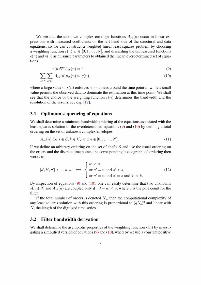
We see that the unknown complex envelope functions Ask(n) occur in linear ex-pressions with measured coefficients on the left hand side of the structural and dataequations, so we can construct a weighted linear least squares problem by choosinga weighting function r(n), n ∈ [0, 1, . . . , N ], and discarding the unmeasured functionsε(n) and ν(n) as nuisance parameters to obtained the linear, overdetermined set of equa-tions

r(n)∇qAsk(n) ≈ 0 (9)∑s∈S

∑k∈Ks

Ask(n)psk(n) ≈ y(n), (10)

where a large value of r(n) enforces smoothness around the time point n, while a smallvalue permits the observed data to dominate the estimation at this time point. We shallsee that the choice of the weighting function r(n) determines the bandwidth and theresolution of the results, see e.g, [12].

3.1 Optimum sequencing of equationsWe shall determine a minimum bandwidth ordering of the equations associated with theleast squares solution of the overdetermined equations (9) and (10) by defining a totalordering on the set of unknown complex envelopes

Ask(n) for s ∈ S, k ∈ Ks and n ∈ [0, 1, . . . , N ] . (11)

If we define an arbitrary ordering on the set of shafts S and use the usual ordering onthe orders and the discrete time points, the corresponding lexicographical ordering thenworks as

[s′, k′, n′] < [s, k, n] ⇐⇒

n′ < n,

or n′ = n and s′ < s,

or n′ = n and s′ = s and k′ < k.

(12)

By inspection of equations (9) and (10), one can easily determine that two unknownsAs′k′(n′) and Ask(n) are coupled only if |n′ − n| ≤ q, where q is the pole count for thefilter.

If the total number of orders is denoted No, then the computational complexity ofany least squares solution with this ordering is proportional to (qNo)

2 and linear withN , the length of the digitized time series.

3.2 Filter bandwidth derivationWe shall determine the asymptotic properties of the weighting function r(n) by investi-gating a simplified version of equations (9) and (10), whereby we use a constant positive

7

real value of r, and a single order with zero shaft speed and an observed response timehistory which is a stationary phasor with frequency ω.

r∇qA(n) ≈ 0, (13)1A(n) ≈ exp(2πinω). (14)

The least squares steady state solution must be a complex multiple of the phasor, sayA exp(2πinω) and so, we have the relation

(r2(exp(2πiω)− 1)q(exp(−2πiω)q − 1) + 1)A = 1, (15)

or, rearranged,

A = (1 + r2(2− 2 cos(2πω))q)−1. (16)

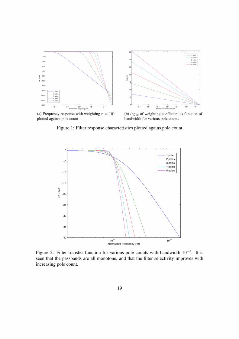
The amplitude of A, as a function of frequency, represents the selectivity of the filteraway from the center frequency, and may be regarded as the transfer function of thefilter. Note that the phase is zero, so this filter has no phase bias. The transfer functionis plotted in Figure (1a) as a function of frequency for various values of the differenceoperator and the weighting r set to 104. In order to choose the weighting which gives a3dB roll off at a selected bandwidth h, we appeal to equation (16), let A = 1/

√2, and

solve for r, giving

r =

√ √2− 1

(2(1− cos(2πω)))q. (17)

This expression is the same as found by Tuma, see e.g., [12], but it appears that thecurrent derivation is novel and simpler as well. The weighting factor is plotted logarith-mically in Figure (1b), whereby it is seen that its dynamic range quickly exceeds themantissa of approximately 16 decimal digits in IEEE double precision floating point.Some of the consequences of this excessive dynamic range will be investigated more indetail in the section on the least squares QR solution scheme. By plotting the transferfunctions of the Vold-Kalman filter for a fixed bandwidth selection and the lowest polecounts, Figure (2), we see that the filters are monotone and that the filter selectivityimproves with increasing pole count. By inspection of the structural equation (9), wesee that there is a totality of No(N + 1) scalar difference equations so it is possible,and often desirable, to apply a separate weighting function rsk(n) for each order, forexample, to enforce a frequency proportional bandwidth to each order when the shaftspeeds have a high dynamic range.

8

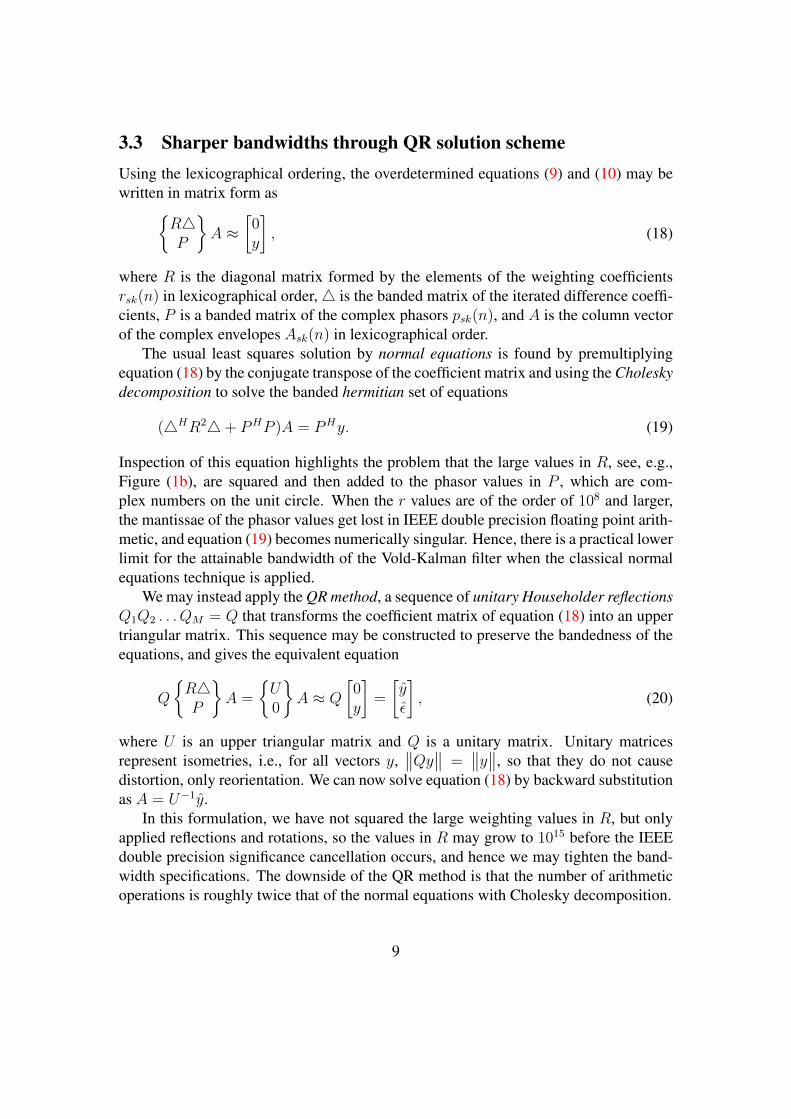
3.3 Sharper bandwidths through QR solution schemeUsing the lexicographical ordering, the overdetermined equations (9) and (10) may bewritten in matrix form as{

R4P

}A ≈

[0y

], (18)

where R is the diagonal matrix formed by the elements of the weighting coefficientsrsk(n) in lexicographical order,4 is the banded matrix of the iterated difference coeffi-cients, P is a banded matrix of the complex phasors psk(n), and A is the column vectorof the complex envelopes Ask(n) in lexicographical order.

The usual least squares solution by normal equations is found by premultiplyingequation (18) by the conjugate transpose of the coefficient matrix and using the Choleskydecomposition to solve the banded hermitian set of equations

(4HR24+ PHP )A = PHy. (19)

Inspection of this equation highlights the problem that the large values in R, see, e.g.,Figure (1b), are squared and then added to the phasor values in P , which are com-plex numbers on the unit circle. When the r values are of the order of 108 and larger,the mantissae of the phasor values get lost in IEEE double precision floating point arith-metic, and equation (19) becomes numerically singular. Hence, there is a practical lowerlimit for the attainable bandwidth of the Vold-Kalman filter when the classical normalequations technique is applied.

We may instead apply the QR method, a sequence of unitary Householder reflectionsQ1Q2 . . . QM = Q that transforms the coefficient matrix of equation (18) into an uppertriangular matrix. This sequence may be constructed to preserve the bandedness of theequations, and gives the equivalent equation

Q

{R4P

}A =

{U0

}A ≈ Q

[0y

]=

[yε

], (20)

where U is an upper triangular matrix and Q is a unitary matrix. Unitary matricesrepresent isometries, i.e., for all vectors y,

∥∥Qy∥∥ =∥∥y∥∥, so that they do not cause

distortion, only reorientation. We can now solve equation (18) by backward substitutionas A = U−1y.

In this formulation, we have not squared the large weighting values in R, but onlyapplied reflections and rotations, so the values in R may grow to 1015 before the IEEEdouble precision significance cancellation occurs, and hence we may tighten the band-width specifications. The downside of the QR method is that the number of arithmeticoperations is roughly twice that of the normal equations with Cholesky decomposition.

9

3.4 Fast single shaft solutionA substantial reduction in computation and storage is possible for the important caseof a single shaft with the same bandwidth specification for all the orders. The basicidea may be found by considering a single order k to be extracted with a correspondingweighting function r(n) and the phasor pk(n) = exp(2πik

∑nl=0 ω(l)).

The overdetermined equations (9) and (10) simplify to

r(n)∇qAk(n) ≈ 0 (21)pk(n)Ak(n) ≈ y(n), (22)

where equation (22) may be rewritten as

1Ak(n) ≈ p−1k (n)y(n), (23)

whereby it is seen that the left hand side becomes that of a phasor of constant frequencyzero, and a time variant zoom transformation on the right hand side. The coefficientmatrix is then of length N + 1, and semi-bandwidth q + 1. If we now denote the set oforders to be extracted as [k1, k2, . . . , kK ], the equations to be solved will have the singleorder independent left hand side, with K right hand sides of the form p−1kj

(n)y(n), forkj ∈ [k1, k2, . . . , kK ]. The inverses of the phasor functions may always be applied, sincethe absolute value of any phasor is always 1.

4 Examples

4.1 A numerical example highlighting the advantages of the QRleast squares solution

This example is purely contrived in order to demonstrate how the QR decompositionmethod can be superior to the Cholesky decomposition for difficult order tracking prob-lems. We construct a scenario where there are three shafts with orders and speed profilesas summarized in table (1).

All orders have a constant amplitude of one, but with a random phase lag. The ordersfor shaft #2 simulate a sideband condition, with four orders separated by 0.0002 of anorder. The constant frequency orders could represent electrical network noise.1 Theexperiments lasted ten seconds, and the data was sampled with a sampling frequency of8 192 Hz. The individual orders were first accumulated per shaft, then summed into asingle time history of sinusoids, and finally, Gaussian noise with a standard deviationof 2, was added to represent the purely indeterministic component of the signal. Figure(3) shows an overlay of the signals with the order time histories belonging to each of

1Groundloops happen to the best of experimentalists, but they do not willingly talk about it

10

Table 1: Speeds and orders for a three shaft numerical example. Shaft #2 simulates anorder with sideband modulation.

Shaft Min Speed Max Speed Type Direction Orders

1 500 1000 Linear Descending [0.8, 1.0, 1.3, 1.5]2 500 1100 Log Ascending [1.000, 1.0002, 1.0004, 1.0006]3 550 550 Const [1.0, 1.24, 1.47, 1.71, 1.94, 2.18]

the three shafts. The plot shows how the dense sidebands of shaft #2 generate a nonperiodic beating over the observation window. The waterfall of frequency versus timefor the total signal is shown in Figure (4), where a red order cursor indicates the beatingof the close orders of the second shaft.

We now want to extract all the present orders from the noisy summed signal, and forthe orders generated by shaft #2 we need to specify a bandwidth of no larger than 0.01 %of an order. We form the least squares equations and solve with both the QR and theclassical Cholesky algorithm in IEEE double precision floating point arithmetic. Theresulting estimated order amplitudes are shown in Figure (5), whereby it in evident thatthe QR results (5a) are reasonable, whereas the Cholesky algorithm (5b) fails due tonumerical error. Inspection of Figure (5a) further indicates that in spite of the narrowbandpass filter, background noise is still present in the order estimates by approximately10 % relative error. As a final check, we tighten the filter bandwidth to 0.001 % andapply the QR algorithm to both the noisy and the clean signal. Figure (6a) shows therelative error is down to approximately 4 % for the noisy signal, whereas the error in theclean signal, (6b), is miniscule.

We can decide to extract the densely clustered orders of shaft #2 as a single entity bywidening the bandwidth to 1% of an order. We filter both the clean and the noisy signaland find that both the QR and Cholesky algorithms give the same results with this widerbandwidth setting. Figure (7) shows the well separated orders are still estimated withtheir unit amplitude, while the the sidebands from shaft #2 are now collected into theenvelope of the beating signal. Furthermore, comparison of Figures (7a) and (7b) showthat the broadband Gaussian noise still contaminates the filtered bands to some extent.

4.2 Force variation caused by eccentricity in Cold Rolling Steel MillFigure (8) shows a schematic of the rolling mill in the example, with Figure (9) depictinga generic stack of work rolls and backup rolls.

In any rolling process, the consistency of the force at a given unit speed is alwayscritical to insure there is a uniform rolled thickness in the end product. Variations in

11

the thickness or gauge of the product can result from inconsistencies in applied forceat a given speed, which can cause for product rejection depending on the severity. Thiscan also cause issues in the downstream processes where consistent formability of theproduct is a must. Out of roundness or eccentricity of rolls is frequently at the root ofsuch issues but since the roll diameters are very closely matched as a practice, beingable to accurately identify the offending roll can be very difficult if not impossible us-ing conventional spectrum analysis methods. To compound the issue, speeds are oftenvarying throughout the process and other control variables including force and tensionare also frequently changing while rolling material. For this reason if spectral resolu-tion is increased to the point that the discrete frequencies of the individual rolls can bedistinguished, the data has typically become excessively smeared and is not usable dueto the transient nature of the rolling process. The fusion of the neighbouring orders maybe seen in the waterfall plot of Figure (10), or equivalently in colour intensity (11). Incontrast, by using the Vold-Kalman, it becomes possible to track through any process orcontrol changes that may occur and accurately identify the offending roll in a fast andefficient manner.

Figure (12) shows an overlay of time histories of the extracted orders, whereby itis clear that the top backup roll is contributing the bulk of the rolling force fluctuation.The speed independent behaviour of the orders indicate a pure kinematics root cause,such as eccentricity or out of round.

4.3 Dual rotor propulsion unit in wind tunnelRecent renewed interest in counter-rotating open rotor propulsion systems has drivenseveral model scale wind tunnel tests. The NASA Open Rotor Propulsion Rig (ORPR)was used as the drive system for one such test done in collaboration with General Elec-tric (GE), see e.g., [16]. The rig consists of two counter rotating spools with a non-rotating center shaft. Each of the two counter rotating spools is attached to a two-stageair turbine on the aft end that can produce up to 560 kW (750 HP). This rig was operatedin a low-speed test campaign from late 2009 to late 2010 in the 9x15 Low Speed WindTunnel at NASA Glenn. The refurbished ORPR installed in the 9x15 wind tunnel isshown in Figure (13). The rotor shown in the figure is a two decades old prototype thatwas chosen by NASA for public domain baseline research [17, 18].

While the speed of the rig is controlled by a feedback controller, the rotation rateof the two rotors varies slightly and the phase is not locked between the rotors. Thismakes the two rotors behave slightly incoherently, and therefore, each rotor has its owndiscernible signature, which allows the Vold-Kalman filter to extract the individual con-tribution of the rotors. A chart of the rotation speed measured for the two rotors is shownin Figure (14).

Microphone and tachometer data were analyzed at 100 KHz sampling rate, and or-ders 10 through 100 relative to each rotor were extracted as time histories. The front

12

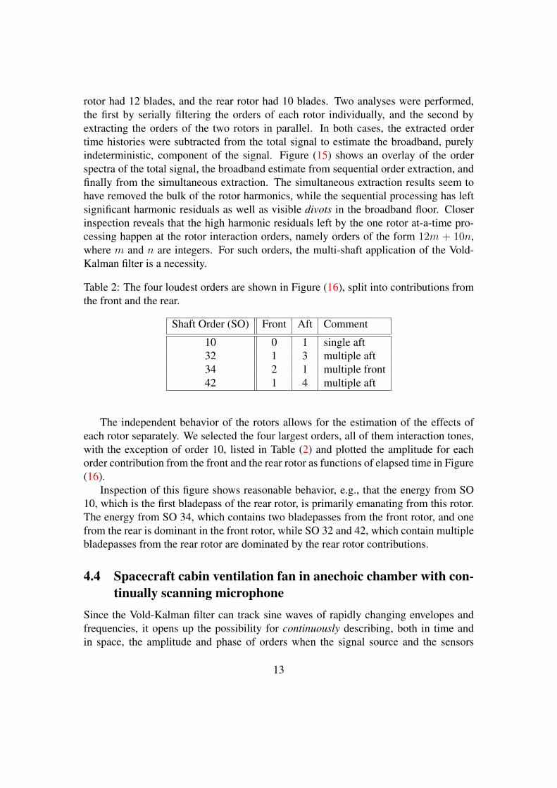
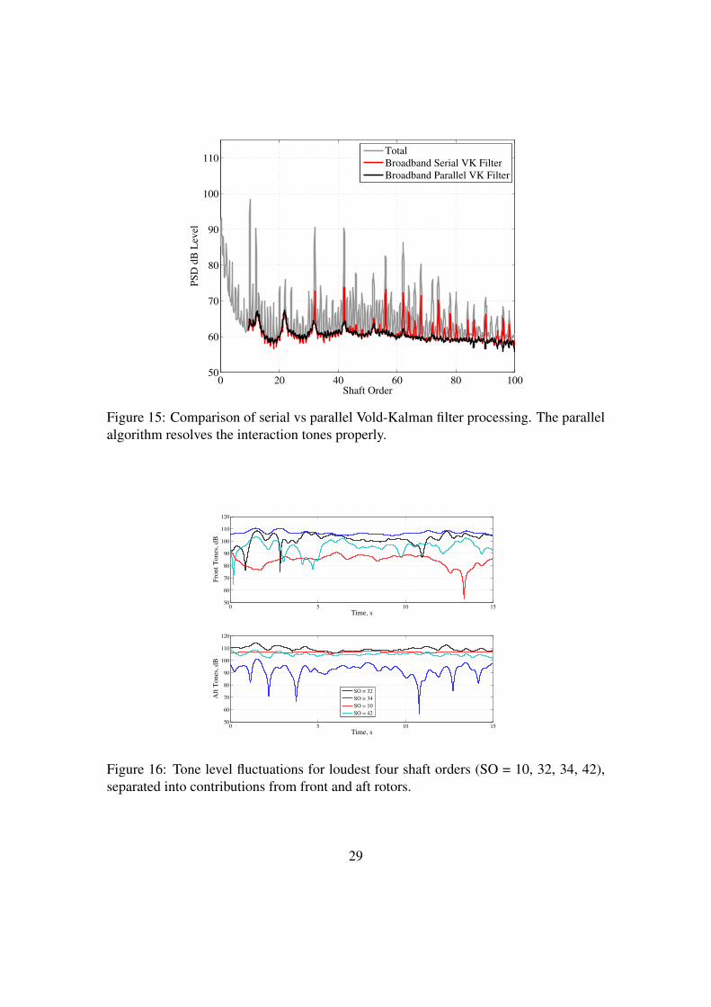
rotor had 12 blades, and the rear rotor had 10 blades. Two analyses were performed,the first by serially filtering the orders of each rotor individually, and the second byextracting the orders of the two rotors in parallel. In both cases, the extracted ordertime histories were subtracted from the total signal to estimate the broadband, purelyindeterministic, component of the signal. Figure (15) shows an overlay of the orderspectra of the total signal, the broadband estimate from sequential order extraction, andfinally from the simultaneous extraction. The simultaneous extraction results seem tohave removed the bulk of the rotor harmonics, while the sequential processing has leftsignificant harmonic residuals as well as visible divots in the broadband floor. Closerinspection reveals that the high harmonic residuals left by the one rotor at-a-time pro-cessing happen at the rotor interaction orders, namely orders of the form 12m + 10n,where m and n are integers. For such orders, the multi-shaft application of the Vold-Kalman filter is a necessity.

Table 2: The four loudest orders are shown in Figure (16), split into contributions fromthe front and the rear.

Shaft Order (SO) Front Aft Comment

10 0 1 single aft32 1 3 multiple aft34 2 1 multiple front42 1 4 multiple aft

The independent behavior of the rotors allows for the estimation of the effects ofeach rotor separately. We selected the four largest orders, all of them interaction tones,with the exception of order 10, listed in Table (2) and plotted the amplitude for eachorder contribution from the front and the rear rotor as functions of elapsed time in Figure(16).

Inspection of this figure shows reasonable behavior, e.g., that the energy from SO10, which is the first bladepass of the rear rotor, is primarily emanating from this rotor.The energy from SO 34, which contains two bladepasses from the front rotor, and onefrom the rear is dominant in the front rotor, while SO 32 and 42, which contain multiplebladepasses from the rear rotor are dominated by the rear rotor contributions.

4.4 Spacecraft cabin ventilation fan in anechoic chamber with con-tinually scanning microphone

Since the Vold-Kalman filter can track sine waves of rapidly changing envelopes andfrequencies, it opens up the possibility for continuously describing, both in time andin space, the amplitude and phase of orders when the signal source and the sensors

13

are in relative motion. Such continuous scans then can then form the basis for bothbeamforming and acoustic holography procedures for stationary sound fields where thesource and sensors are in relative motion. Our example will outline parts of a procedureto map the sound fields generated by the orders of a ducted fan in an anechoic chamber.

To provide a safe and productive soundscape in manned spacecraft, NASA has re-cently tested prototype cabin ventilation fans in the Glenn Research Center, see e.g,[19, 20, 21].

We used a dataset from an experiment in NASA Glenn’s Acoustic Test Lab, wherethe test specimen was a ducted axial fan, shown in Figure (17). In our configuration,the fan was 9 inches long and 4 inches in diameter, and it was mounted on a pedestal onthe laboratory floor. In addition to 4 stationary microphones and a tachometer on thefan shaft, a traversing array of microphones was mounted on an overhead track whichallowed for 168 inches of horizontal travel, and a fixed vertical distance of 41 inches. Aphoto of sample setup with a much closer vertical distance is shown in Figure (18). Theschematic view in Figure (19) shows the testing Glenn Acoustical Test Lab configura-tion for these tests.The fan speed was set to 12 000 RPM, and after transients had died,the array was set to traverse at a constant speed of 1 inch per second.

The dominant bladepass orders were filtered out with the Vold-Kalman filter fromthe time record of the middle traversing microphone, and the corresponding Wold de-composition into sinusoids and broadband noise is shown in Figure (20). A qualitativeinspection of this figure indicates that the amplitude of the blade harmonics is larger onthe exhaust side of the fan (positive abscissa values). To assess the dimensionality ofthe sound field, the eigenvalues of the autospectral matrix2 of the four stationary mi-crophones were plotted as a function of frequency in the range 1 kHz–6 kHz in Figure(21). It was evident that the three first bladepass harmonics were dominant self-coherentsound fields, while for each frequency band, there were several mutually incoherentbroadband sound fields composed of flow noise.

The real part of the complex envelope of the second bladepass order at 3.6 kHz wasplotted as a function of traverse distance in Figure (22). This plot also shows in redthe result of a conventional fixed index scan with a 3 inch spacing between samplinglocations. The fixed index data compare well at the sampling points, but spatial aliasingis evident toward the ends of the traverse interval; the acoustic wavelength at this orderbeing 3.7 inches. As is to be expected, the amplitude of this rotor order is larger on theexhaust side of the fan.

Since we can escape the curse of spatial aliasing along scan paths, the tools ofFourier acoustics will often allow us to base a spatial reconstruction of a self-coherentacoustic field from the measurements along paths. For example, we used the secondbladepass order evaluated along a straight line, assumed axisymmetry with respect tothe centerline of the fan and thereby obtained the contour plot of the sound field in

2This is often called the Proper Orthogonal Decomposition (POD).

14

Figure (23), where the space fan and the microphone traverse path are also indicated.The resolution of the reconstruction is limited by the acoustic wavelength since theevanescent components have decayed by the time they reach the traversing microphone.The sound field reconstruction was created by Fourier acoustic techniques gleaned fromacoustic holography [22, 23].

It is worth noticing that the Vold-Kalman filter has been used in the past to trackengine orders from both moving ground vehicles and aircraft, see, e.g. [24, 25, 26, 27,28, 29].

5 ConclusionsThe new lexicographical ordering of the Vold-Kalman equations allows for the efficientsolution of large and complex order tracking problems with multiple shaft, using directsolution schemes in a relatively short amount of time. The bottleneck now has becomeone of memory space rather than processor cycles. Since memory prices are steadilydecreasing and slower mechanical storage is being supplanted by solid state drives, thetime seems to be right for widespread application of the Vold-Kalman filter.

The reformulation of the least squares solution in terms of the sparse QR decompo-sition exploits the dynamic range of the IEEE douple precision floating point arithmetic,and permits narrower bandwidths than previously achieved with the normal equationsmethod and the Cholesky decomposition.

6 AcknowledgementsThe author would like to thank Dr. David Stephens of NASA Glenn Research Center,Acoustics Branch for the analyses of the counter-rotating open rotor in the 9x15 LowSpeed Wind Tunnel at NASA Glenn, see, e.g, [30]. Thanks are also due to Ms. L.Danielle Koch and Dr. Daniel Sutliff of the same department for guidance and contin-uous scan data acquisition on the ducted spacecraft cabin ventilation fan in the NASAGlenn Acoustic Test Laboratory. All three have also contributed images shown in thispaper.

Thanks are also extended to Drs. Parthiv Shah and Michael Yang of ATA Engineer-ing, Inc.

The algorithms were coded in Matlab and GNU Octave [31, 32] for which rudimen-tary implementations of the Vold-Kalman filter are available in open source form. Therolling mill example was computed with the commercial ibaRotate program [33].

15

7 Bibliography

References[1] H. Niemi, On the construction of the wold decomposition for non-stationary

stochastic processes, Probability and Math. Statistics,-1980.-1.-Fasc 1 (1980) 73–82.

[2] H. Niemi, On the construction of wold decomposition for multivariate stationaryprocesses, Journal of Multivariate Analysis 9 (4) (1979) 545–559.

[3] H. Wold, A study in the analysis of stationary time series, Ph.D. thesis, Stockholm(1938).

[4] H. Vold, J. Leuridan, High resolution order tracking at extreme slew rates, usingkalman tracking filters, SAE paper 931288.

[5] H. Herlufsen, S. Gade, H. Konstantin-Hansen, H. Vold, Characteristics of the vold-kalman order tracking filter, in: Acoustics, Speech, and Signal Processing, 2000.ICASSP’00. Proceedings. 2000 IEEE International Conference on, Vol. 6, IEEE,2000, pp. 3895–3898.

[6] H. Vold, M. Mains, J. Blough, Theoretical foundations for high performance ordertracking with the vold-kalman tracking filter, SAE paper 972007.

[7] H. Vold, H. Herlufsen, M. Mains, D. Corwin-Renner, Multi axle order trackingwith the vold-kalman tracking filter, Sound and Vibration 31 (5) (1997) 30–35.

[8] H. Vold, P. Shah, J. Davis, P. Bremner, D. McLaughlin, P. Morris, J. Veltin,R. McKinley, High-resolution continuous scan acoustical holography applied tohigh-speed jet noise, AIAA 2010-3754, 2010.

[9] K. Wang, P. S. Heyns, The combined use of order tracking techniques for enhancedfourier analysis of order components, Mechanical systems and signal processing25 (3) (2011) 803–811.

[10] K. Wang, P. S. Heyns, Application of computed order tracking, vold–kalman fil-tering and emd in rotating machine vibration, Mechanical Systems and Signal Pro-cessing 25 (1) (2011) 416–430.

[11] G. H. Golub, C. F. Van Loan, Matrix computations, Vol. 3, Johns Hopkins Univer-sity Press, 1996.

16

[12] J. Tuma, Setting the passband width in the vold-kalman order tracking filter, in:12th International Congress on Sound and Vibration,(ICSV12), Lisboa, 2005.

[13] D. B. Stephens, H. Vold, Order tracking signal processing for open rotor acoustics,to be submitted for publication in Journal of Sound and Vibration (1 2013).

[14] H. Vold, B. Schwarz, M. Richardson, Measuring operating deflection shapes un-der non. stationary conditions, in: Proceedings of International Modal AnalysisConference XVIII, 2000.

[15] R. E. Kálmán, A new approach to linear filtering and prediction problems, Trans-actions of the ASME, Journal of Basic Engineering, 82 (Series D): 35–45. 82(March 1960) 35–45.

[16] D. B. Stephens, E. Envia, Acoustic shielding for a model scale counter-rotationopen rotor, AIAA-2011-2940, 17th AIAA/CEAS Aeroacoustics Conference, Port-land, Oregon, USA.

[17] D. M. Elliott, Initial Investigation of the Acoustics of a Counter-Rotating OpenRotor Model with Historical Baseline Blades in a Low-Speed Wind Tunnel, Na-tional Aeronautics and Space Administration, Glenn Research Center, 2012.

[18] D. Van Zante, J. Gazzaniga, D. Elliott, R. Woodward, An open rotor test case:F31/a31 historical baseline blade set, ISABE-2011, September (2011) 12–16.

[19] L. D. Koch, T. D. Shook, D. T. Astler, S. A. Bittinger, Tone noise predictions fora spacecraft cabin ventilation fan ingesting distorted inflow and the challenges ofvalidation.

[20] L. D. Koch, C. A. Brown, T. D. Shook, J. Winkel, J. S. Kolacz, D. M. Podboy,R. A. Loew, J. H. Mirecki, Acoustic measurements of an uninstalled spacecraftcabin ventilation fan prototype.

[21] L. D. Koch, Quiet, efficient fans for spacecraft: An overview of nasa’s technologydevelopment plan, in: INTER-NOISE and NOISE-CON Congress and ConferenceProceedings, Vol. 2010, Institute of Noise Control Engineering, 2010, pp. 583–592.

[22] J. D. Maynard, E. G. Williams, Y. Lee, Nearfield acoustic holography: I. theory ofgeneralized holography and the development of NAH, The Journal of the Acous-tical Society of America 78 (1985) 1395.

[23] E. G. Williams, Fourier acoustics: sound radiation and nearfield acoustical holog-raphy, academic press, 1999.

17

[24] Shah, Parthiv N and Vold, Håvard and Hensley, Dan and Envia, Edmane andStephens, David, A High-Resolution Continuous-Scan Acoustic MeasurementMethod for Turbofan Engine Applications, Journal of Turbomachinery, 137 (12)(2015)

[25] Vold, Havard I., and Parthiv N. Shah. Methods and apparatus for high-resolutioncontinuous scan imaging using vold-kalman filtering., U.S. Patent No. 9,482,644.1 Nov. 2016.

[26] J. Tuma, Dedopplerisation in vehicle external noise measurements, in: Proc. 11thInternational Congress on Sound and Vibration, St. Petersburg, 2004.

[27] J. Tuma, Gearbox noise and vibration prediction and control, International Journalof Acoustics and Vibration 14 (2) (2009) 99–108.

[28] P. Pelant, J. Tuma, T. V. Benes, Kalman order tracking filtration in car noise andvibration measurements, in: Proceedings of the 33rd International Congress andExposition on Noise Control Engineering, Prague, Czech Republic, 2004.

[29] F. Marki, K. Gulyas, F. Augusztinovicz, R. Bisping, M. Bauer, M. Bellmann,H. Remmers, D. Sabbatini, H. Van der Auweraer, K. Janssens, Sound synthesizertool for line sound quality analysis and target sound design of aircraft flyovers, in:Proc. INTER-NOISE, 2011.

[30] Stephens, David B., and Håvard Vold. Order tracking signal processing for openrotor acoustics., Journal of Sound and Vibration 333.16 (2014): 3818-3830.

[31] http://www.mathworks.com

[32] https://www.gnu.org/software/octave/

[33] http://www.iba-ag.com/en/ibarotate/

8 Figures

18

10−5

10−4

10−3

10−2

10−1

−220

−200

−180

−160

−140

−120

−100

−80

−60

−40

−20

0

dB

rollo

ff

Normalized Frequency (Hz)

1 pole

2 poles

3 poles

4 poles

5 poles

(a) Frequency response with weighting r = 104

plotted against pole count

10−8

10−7

10−6

10−5

10−4

10−3

10−2

0

5

10

15

20

25

30

35

log

10(r

)

Normalized Bandwidth (Hz)

1 pole

2 poles

3 poles

4 poles

5 poles

(b) log10 of weighting coefficient as function ofbandwidth for various pole counts

Figure 1: Filter response characteristics plotted agains pole count

10−5

10−4

−40

−35

−30

−25

−20

−15

−10

−5

0

dB

ro

lloff

Normalized Frequency (Hz)

1 pole

2 poles

3 poles

4 poles

5 poles

Figure 2: Filter transfer function for various pole counts with bandwidth 10−5. It isseen that the passbands are all monotone, and that the filter selectivity improves withincreasing pole count.

19

Figure 3: Wold decomposition of synthetic noisy signal. Overlay of orders per shaftplus the sum of all orders. Notice the modulation of the sideband orders of shaft #2.

20

Figure 4: Waterfall plot of frequency vs. elapsed time for the accumulated time historyof all orders and noise as shown in Figure (3). The red order cursor tracks the sidebandmodulation due to shaft #2. The added Gaussian noise is evident in the rough texture ofthe noise floor.

0 2 4 6 8 100.85

0.9

0.95

1

1.05

1.1

Time (s)

Am

plitu

de

(a) QR decomposition estimates with 10% rela-tive error. The smooth curves belong to shaft #2.

0 2 4 6 8 10

2

4

6

8

10

12

14

16

18

20

Time (s)

Am

plitu

de

(b) Cholesky decomposition gives nonsense re-sults

Figure 5: Amplitudes of all orders estimated with bandwidth 0.01% of an order

21

0 2 4 6 8 10

0.96

0.97

0.98

0.99

1

1.01

1.02

1.03

1.04

Time (s)

Am

pli

tud

e

(a) QR decomposition estimates with 4% relativeerror. The smooth curves belong to shaft #2.

0 1 2 3 4 5 6 7 8 9 10

0.99

0.992

0.994

0.996

0.998

1

1.002

1.004

1.006

1.008

Time (s)

Am

plit

ude

(b) No significant error on noise free signal

Figure 6: Amplitudes of all orders estimated with bandwidth 0.001% of an order

0 2 4 6 8 10

0.5

1

1.5

2

2.5

3

3.5

Time (s)

Am

plitu

de

(a) Estimates on noisy signal error

0 1 2 3 4 5 6 7 8 9 10

0.5

1

1.5

2

2.5

3

3.5

Time (s)

Am

plit

ude

(b) No significant error on noise free signal

Figure 7: Amplitudes of all orders estimated with bandwidth 1% of an order. Note thatthe curves in red now represent the beating amplitude of the cluster of bands from shaft#2.

22

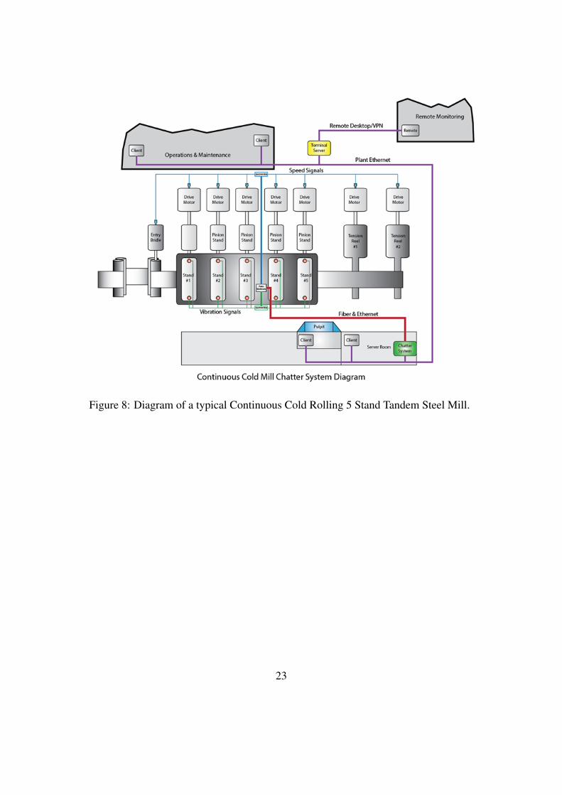
Figure 8: Diagram of a typical Continuous Cold Rolling 5 Stand Tandem Steel Mill.

23

Figure 9: Diagram of a typical stack of work rolls and backup rolls.

24

Figure 10: Waterfall plot of frequency vs. elapsed time for the Total Rolling Force signalon the Tandem Mill #4 Stand. The red cursors track the 1st, 2nd, and 3rd order for theTop Backup Roll with the 1st order being the most significant. You can note that the useof standard spectral analysis is incapable of separating the individual frequencies of theTop and Bottom Backup Rolls. This is because the speeds are not constant. Thereforeincreasing the resolution to differentiate between the two discrete sources results inexcessive smearing that renders the results unusable. Hence, the need for applying theVold-Kalman Filter.

25

Figure 11: Contour plot of frequency vs elapsed time for the Total Rolling Force signalon the Tandem Mill #4 Stand. In this form it is clear that the graphical resolution isinsufficient to separate the rolling force contribution from the top and bottom backuprolls.

26

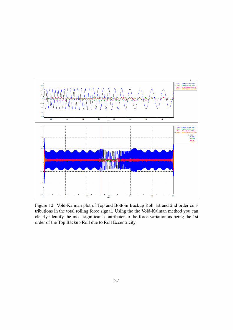
Figure 12: Vold-Kalman plot of Top and Bottom Backup Roll 1st and 2nd order con-tributions in the total rolling force signal. Using the the Vold-Kalman method you canclearly identify the most significant contributer to the force variation as being the 1storder of the Top Backup Roll due to Roll Eccentricity.

27

Figure 13: Open Rotor Propulsion Rig in 9x15 Wind Tunnel at NASA Glenn ResearchCenter. NASA Image C-2010-3602.

0 5 10 15110.2

110.25

110.3

110.35

110.4

110.45

110.5

110.55

110.6

110.65

110.7

Time, Seconds

Sh

aft

Rate

, H

z

Front Rotor

Aft Rotor

Figure 14: Sample rotation speed traces in Hertz for 15 second data record.

28

0 20 40 60 80 10050

60

70

80

90

100

110

Shaft Order

PS

D d

B L

evel

Total

Broadband Serial VK Filter

Broadband Parallel VK Filter

Figure 15: Comparison of serial vs parallel Vold-Kalman filter processing. The parallelalgorithm resolves the interaction tones properly.

0 5 10 1550

60

70

80

90

100

110

120

Time, s

Fro

nt

Tones,

dB

0 5 10 1550

60

70

80

90

100

110

120

Aft

Tones,

dB

Time, s

SO = 32

SO = 34

SO = 10

SO = 42

Figure 16: Tone level fluctuations for loudest four shaft orders (SO = 10, 32, 34, 42),separated into contributions from front and aft rotors.

29

Figure 17: Transparency view of ducted spacecraft ventilation fan. Image courtesy ofNASA.

30

Figure 18: The spacecraft cabin ventilation fan and the traversing microphones in theNASA Glenn Acoustical Test Lab.

31

CD-12-83321

Figure 19: Schematic view of the test setup in the NASA Glenn Acoustical Test Lab.

32

Figure 20: Wold decomposition of microphone time history into broadband noise andharmonic components, The exhaust direction is to the right of the plot.

33

1 1.5 2 2.5 3 3.5 4 4.5 5 5.5 6Frequency (kHz)

Lo

g A

mp

litu

de

Primary

Secondary

Tertiary

4th

Figure 21: Eigenvalues (POD) of autospectral matrix of the reference microphones. Thethree largest peaks are the first three bladepass harmonics (9/rev, 18/rev and 27/rev).Several significant mutually incoherent broadband fields are indicated between thetones. Imperfections in the fan and duct asymmetries give rise to secondary tones inaddition to the bladepass harmonics.

34

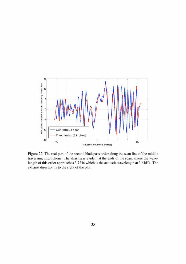
Figure 22: The real part of the second bladepass order along the scan line of the middletraversing microphone. The aliasing is evident at the ends of the scan, where the wave-length of this order approaches 3.72 in which is the acoustic wavelength at 3.6 kHz. Theexhaust direction is to the right of the plot.

35

Figure 23: Contour plot of the acoustic field generated by the second bladepass order ofthe spacecraft cabin ventilation fan at 3.6 kHz. The fan is located below the plot, withblow direction to the right. The horizontal path of the scanning microphone is indicatedat the top of the figure, 40 inches from the fan centerline.

36