the viscosity of n-decane to high temperatures of 573 k and high pressures of 300 mpa

Z. Phys. Chem.216 (2002) 1295–1310 by Oldenbourg Wissenschaftsverlag, München

The Viscosity of n-Decane to HighTemperatures of 573 K and High Pressuresof 300 MPa

By Lutz-Dieter Naake1, Gabriele Wiegand2 and Ernst Ulrich Franck3,∗1 Present Address: Degussa AG, Konzernbereich Umwelt, Sicherheit, Gesundheit,

Qualität, Bennigsenplatz 1, D-49474 Düsseldorf, Germany2 Present Address: Forschungszentrum Karlsruhe GmbH, ITC-CPV, Postfach 3640,

D-76021 Karlsruhe, Germany3 Universität Karlsruhe, Institut fuer Physikalische Chemie, Postfach 6980,

D-76128 Karlsruhe, Germany

(Received December 20, 2001; accepted in revised form May 22, 2002)

Viscosity / n-Decane / High Temperature / High Pressure

The dynamic viscosity of liquidn-decane has been measured with the “Oscillating DiskMethod” from 293 K to 573 K and from 0.1 MPa to 300 MPa. A high pressure autoclaveof 50 mm internal diameter contained between two rigid disks an oscillating stainless steeldisk of 44 mm diameter suspended on a platinum-tungsten wire. Pressure was generatedwith a spindle press filled with a suitable hydraulic fluid separated from then-decane.Thus heating and pressure variation could be performed at selected constant volumes.The density dependence of the viscosity could be determined.

The viscosity increases at 373 K from 375 to 1602µPa s in the pressure range from0.1 to 200 MPa, at 473 K from 200 to 1114µPa s in the pressure range from 10 to300 MPa, and at 573 K from 223 to 675µPa s in the pressure range from 60 to 300 MPa.The mean accuracy of the viscosity measurements is about 1.3%. A polynomial functiondescribing the viscosity variation with pressure and temperature is given. The maximumaverage deviation is 0.46%, the mean average deviation between measured and calculateddata is 0.11%. The viscosity as a function of density is also shown. With Arrhenius plots,the energies of activation are obtained.

1. IntroductionAmong transport properties of fluids the viscosity is of special interest. It isa particularly useful basis for the theoretical treatment of kinetic phenomenain fluids. Its technical importance is obvious. The viscosity of liquids is de-pending on density, which is interesting to investigate. It was the intention

* Corresponding author. E-mail: [email protected]

1296 L.-D. Naakeet al.

of the present work to perform such investigations with a liquid of long lin-ear molecules liken-decane, which can be considered as a model fluid forother linear hydrocarbons with technical interest. The critical temperature ofn-decane is high (Tc = 617.6 K). Measurements had to be restricted to 573 Kand thus referred to the liquid state only. At such conditions, the compress-ibility is relatively low, and in order to cover a somewhat extended range ofdensity, high pressures to 300 MPa have been applied.

Different methods to measure the viscosity of fluids with reasonable adapt-ability and accuracy have been described in the literature [1]. For the presentpurpose, the viscometer must fit into an autoclave and operate at conditions ofhigh temperature and high pressure to determine absolute viscosities around0.001 Pa s with an accuracy better than 2%. The oscillation method appearedto be best suited. A rotationally symmetric body suspended on a thin wire per-forms rotational oscillations in the fluid. Their attenuation determines the fluidviscosity. The oscillating body can be a cylinder, a sphere or a flat disk. Theobservation of an oscillating disk was the method applied [2]. Detailed dis-cussions of the method have been given already in the 19th century [3]. Morerecently, Vogel [4] gave a survey on the oscillating disk method. Macwoodet al. [5, 6] extended the theoretical treatment, which was again improved byKestinet al. [7, 8].

2. ExperimentalCentral part of the apparatus is a cylindrical autoclave with 15 cm o.d. and 5 cmi.d., shown in Fig. 1.

It was made of a nickel-base superalloy1 and was vertically mounted. Thetop is closed with a Bridgman unsupported area seal, from which extends ver-tically a high pressure stainless steel tube. The lower part of the autoclave hasan axial dead end hole of 10 mm diameter. Vertically to the main axis of theautoclave a wide and a narrow bore hole serve to introduce a sapphire window(6) and a thermocouple (1). The upper vertical high pressure tube (42 mm o.d.and 18 mm i.d.) of 317 mm length contains an alumina tube (3) which supportsthe suspended Pt/W torsion wire (2). The packing ring of the Bridgman sealis made of bronze-reinforced teflon (4). It is stable only to 623 K, which lim-its the highest applicable temperature. This also limits the highest applicablepressure to 350 MPa. Below, the autoclave rested on a tapered roller bearing,which permitted to rotate it to a certain degree and to start the inside disk tooscillate. Underneath the oscillating disk is a 97 mm long fixed rod, which car-ries a plane metal mirror (9) as shown in Fig. 1. The mirror reflects a laser beamto determine the disk movement. A tube of sintered alumina of 290 mm lengthand 15 mm o.d. and 6 mm i.d. is mounted within the high pressure tube. Fromthe top of the alumina tube the oscillating wire is suspended, so that, to some

1 Material Number 2.4969

The Viscosity ofn-Decane to High Temperatures of 573 K and High Pressure ...1297

Fig. 1. Scheme of autoclave. 1= thermocouple with high pressure connection, 2= Pt/Wwire, 3 Al2O3 tube, 4 = teflon bronze packing, 5= osciallating stainless steel disk,6 = sapphire window, 7= Nb mounting support, 8= rigid stainless steel disks, 9= metalmirror.

extent, the different thermal expansion of the autoclave tube and the wire canbe compensated. The torsional wire of 300 mm length (2) is suspended withinthe tube. It has a diameter of 127µm and is made of a platinum tungsten alloy(92% Pt, 8% W), an alloy particularly suited because of its high strength andits low hysteresis of oscillation attenuation. At its lower end, within the widesection of the autoclave, it carries the rotationally oscillating steel disk betweentwo rigid steel disks (5) as shown in Fig. 2. The oscillating disk is made of 18/8stainless steel with an outer diameter of 43.75 mm, a height of 3.63 mm anda mass of 42.780 g resulting in a moment of inertia of 10332 g mm2.

A helium-neon gas laser is mounted at 2 m distance from the autoclave andthe beam is reflected from the oscillating mirror. The laser reflex is registeredwith two photo-electronic sensors. These are connected to a 20 MHz counterwith a time resolution of 100 ns. Only every second pulse acted as a switchpulse. A printer recorded the time intervals which yielded the oscillating timet(see below). For a detailed description see [2].

Three external resistance heaters were applied to produce the desired auto-clave temperatures. Among these the third heater served to minimize the heat


Fig. 2. Characteristic data of oscillating system.

flow into the roller bearing at the bottom of the autoclave. The sheathed heat-ing wires were imbedded in grooves in brass half shells. Exact knowledge ofthe temperature distribution was important. Five thermocouples were applied.Three were located inside, close to the disk. Two others recorded the tempera-ture at the top and bottom of the autoclave (see Fig. 1). The accuracy was about±0.25 K. The influence of the alternating magnetic field caused by the electricheating on the oscillating disk was found negligible.

The desired pressure was produced with hand-operated spindle presses to400 MPa, which were filled with a hexane diluted hydraulic oil. An auxiliaryroom temperature autoclave contained an expandable stainless steel bellowswhich separated then-decane sample fluid from the pressure transmitting hy-draulic fluid. The closed end of the bellows carried a 300 mm long thin metallicwire with a small magnetic tip extending into a narrow nonmagnetic high pres-sure tube. The expansion of the bellows can be determined precisely fromoutside from the position of the magnetic tip with an induction bridge. Thusheating and pressure variations at constant sample volume were possible. Pres-sures were measured with different calibrated Bourdon gauges to 16 MPa and300 MPa. The autoclave is connected to the remaining structure with flexi-ble stainless steel tubing of 3.2 mm o.d. and 0.5 mm i.d. in order to permit


limited rotation. When assembling the apparatus, special care was taken to en-sure equal distances between the rigid and the oscillating disks, the horizontalposition of which was also very carefully verified [2]. At the beginning ofthe experimental programme the oscillation time t0 at vacuum conditions hasbeen determined for air at 0.1 MPa as a function of temperature up to 320◦C.Within the given tolerance,t0 in air was set equal to the quantity at vacuumconditions.

3. Results

3.1 Evaluation

Every measurement with the viscometer gives a data pair of the logarithmicdecrement∆ and the oscillation timet. Of at least three such determinationsan average value is obtained. According to the recommendation of Kestinet al.[2, 8] calculation of viscosity is performed with the following equation:

2

Θ

(∆

Θ−∆0

)= m

{H1K2 + H2K1 +

(2d

R

)(H1 + 3δ

2RΘ+ 3δ 2

16R2Θx

)+ E

}

(1)

with

Θ = t/t0, x =

[(∆2 +1

)0.5 −∆]

2Θ

0.5

m = πρR4δ/I β = b/δ

H1 = 3x/2Θ−1/8x3Θ3, H2 = 3/4xΘ2 − x3

K1 = sinY/ coshX −cosY, K2 = sinhX/ coshX −cosY

X = 2βx, Y = β/xΘ

To calculate the viscosity the following quantities are needed:

• The geometric data of the viscometer (b, d, R, I : see Fig. 2)• The vacuum oscillation timet0 as a function of temperature• The intrinsic attenuation∆0 of the torsion wire in vacuum as a function of

temperature• The boundary correction termE as a function ofδΘ• The densityρ of the liquidn-decane at experimental conditions.

The working function (Eq. (1)) can only be solved iteratively. It is solved forthe boundary layer thickness, which is


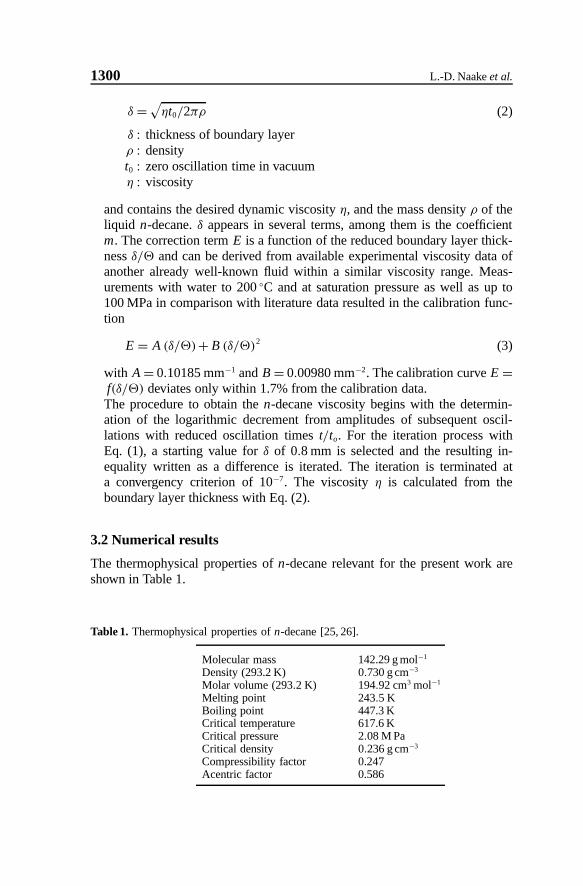
δ = √ηt0/2πρ (2)

δ : thickness of boundary layerρ : densityt0 : zero oscillation time in vacuumη : viscosity

and contains the desired dynamic viscosityη, and the mass densityρ of theliquid n-decane.δ appears in several terms, among them is the coefficientm. The correction termE is a function of the reduced boundary layer thick-nessδ/Θ and can be derived from available experimental viscosity data ofanother already well-known fluid within a similar viscosity range. Meas-urements with water to 200◦C and at saturation pressure as well as up to100 MPa in comparison with literature data resulted in the calibration func-tion

E = A (δ/Θ)+ B (δ/Θ)2 (3)

with A = 0.10185 mm−1 andB = 0.00980 mm−2. The calibration curveE =f(δ/Θ) deviates only within 1.7% from the calibration data.The procedure to obtain then-decane viscosity begins with the determin-ation of the logarithmic decrement from amplitudes of subsequent oscil-lations with reduced oscillation timest/to. For the iteration process withEq. (1), a starting value forδ of 0.8 mm is selected and the resulting in-equality written as a difference is iterated. The iteration is terminated ata convergency criterion of 10−7. The viscosityη is calculated from theboundary layer thickness with Eq. (2).

3.2 Numerical results

The thermophysical properties ofn-decane relevant for the present work areshown in Table 1.

Table 1. Thermophysical properties ofn-decane [25, 26].

Molecular mass 142.29 g mol−1

Density (293.2 K) 0.730 g cm−3

Molar volume (293.2 K) 194.92 cm3 mol−1

Melting point 243.5 KBoiling point 447.3 KCritical temperature 617.6 KCritical pressure 2.08 M PaCritical density 0.236 g cm−3

Compressibility factor 0.247Acentric factor 0.586


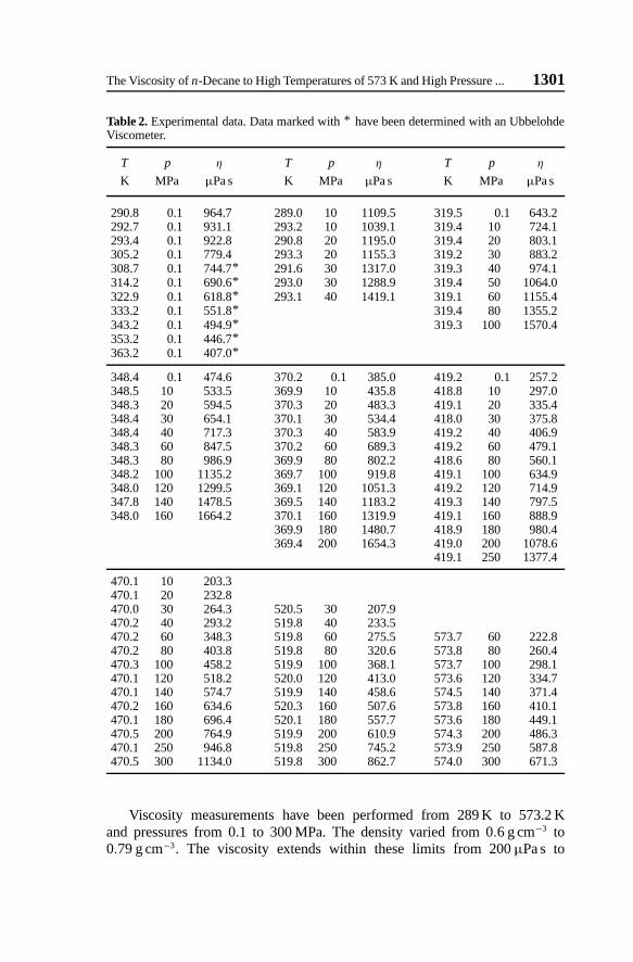
Table 2. Experimental data. Data marked with* have been determined with an UbbelohdeViscometer.

T p η T p η T p η

K MPa µPa s K MPa µPa s K MPa µPa s

290.8 0.1 964.7 289.0 10 1109.5 319.5 0.1 643.2292.7 0.1 931.1 293.2 10 1039.1 319.4 10 724.1293.4 0.1 922.8 290.8 20 1195.0 319.4 20 803.1305.2 0.1 779.4 293.3 20 1155.3 319.2 30 883.2308.7 0.1 744.7* 291.6 30 1317.0 319.3 40 974.1314.2 0.1 690.6* 293.0 30 1288.9 319.4 50 1064.0322.9 0.1 618.8* 293.1 40 1419.1 319.1 60 1155.4333.2 0.1 551.8* 319.4 80 1355.2343.2 0.1 494.9* 319.3 100 1570.4353.2 0.1 446.7*363.2 0.1 407.0*

348.4 0.1 474.6 370.2 0.1 385.0 419.2 0.1 257.2348.5 10 533.5 369.9 10 435.8 418.8 10 297.0348.3 20 594.5 370.3 20 483.3 419.1 20 335.4348.4 30 654.1 370.1 30 534.4 418.0 30 375.8348.4 40 717.3 370.3 40 583.9 419.2 40 406.9348.3 60 847.5 370.2 60 689.3 419.2 60 479.1348.3 80 986.9 369.9 80 802.2 418.6 80 560.1348.2 100 1135.2 369.7 100 919.8 419.1 100 634.9348.0 120 1299.5 369.1 120 1051.3 419.2 120 714.9347.8 140 1478.5 369.5 140 1183.2 419.3 140 797.5348.0 160 1664.2 370.1 160 1319.9 419.1 160 888.9

369.9 180 1480.7 418.9 180 980.4369.4 200 1654.3 419.0 200 1078.6

419.1 250 1377.4

470.1 10 203.3470.1 20 232.8470.0 30 264.3 520.5 30 207.9470.2 40 293.2 519.8 40 233.5470.2 60 348.3 519.8 60 275.5 573.7 60 222.8470.2 80 403.8 519.8 80 320.6 573.8 80 260.4470.3 100 458.2 519.9 100 368.1 573.7 100 298.1470.1 120 518.2 520.0 120 413.0 573.6 120 334.7470.1 140 574.7 519.9 140 458.6 574.5 140 371.4470.2 160 634.6 520.3 160 507.6 573.8 160 410.1470.1 180 696.4 520.1 180 557.7 573.6 180 449.1470.5 200 764.9 519.9 200 610.9 574.3 200 486.3470.1 250 946.8 519.8 250 745.2 573.9 250 587.8470.5 300 1134.0 519.8 300 862.7 574.0 300 671.3

Viscosity measurements have been performed from 289 K to 573.2 Kand pressures from 0.1 to 300 MPa. The density varied from 0.6 g cm−3 to0.79 g cm−3. The viscosity extends within these limits from 200µPa s to


1664µPa s. The lowest and highest oscillation timest observed were be-tween 7.75717 s and 8.02163 s. The logarithmic decrement∆ varied between0.0138604 and 0.0468477. Table 2 gives the original experimental data meas-ured at temperatureT and pressurep.

For every temperature-pressure condition, average values from three inde-pendent determinations of the oscillation time and the logarithmic decrementhave been obtained. Additionally, at normal pressure of 0.1 MPa a number ofmeasurements have been carried out with a thermostatted Ubbelohde capillaryviscometer from 305.2 K up to 363.2 K. The results are marked with asterisksin Table 2. The density at the specific temperature and pressure conditions haveto be known to calculate the viscosity data. All density data have been takenfrom Gehrig and Lentz [9] who covered a range to 673 K and 300 MPa.

3.3 Uncertainty discussion

Different sources of possible uncertainties of the viscosity results have been ex-amined applying the law of error propagation to Eq. (2). Then the relative errorin viscosity is represented by Eq. (4)

Fη,max/η = 2Fδ/δ+ Fρ/ρ+ Ft0/t0 (4)

Fη,max/η : Maximum error of viscosity

Fδ/δ : Error contribution of boundary thickness

Fρ/ρ : Error contribution of density

Ft0/t0 : Error contribution of osciallation time

The thickness of the boundary layerδ (Eq. (2)) is influenced by the characteris-tics of the oscillating system, the decrement of oscillation time determination,the influence of density uncertainties caused by the uncertainties of tempera-ture and pressure measurement.

Table 3 summarizes the contribution of all uncertainties to the mean aver-age deviation (not higher than 1.41%) and the maximum error (not higher than1.72%) of the viscosity.

3.4 Polynomial Approximation

The raw data listed in Table 2 have been processed by a polynomial fittingprocedure given in Eq. (5) for the viscosity as a simultaneous function of tem-perature and pressure.

ln η = a0 +a1 ln T +a2 ln T2 +a4 ln T4 (5)

+b1 p+b2 p2 +b3 p3 +b4 p4

+c1 ln Tp+c2 ln T2 p+c3 ln Tp2 +c4 ln T2 p2


Table 3. Relative error contribution to estimated total errorFη/η in % of experimental vis-cosity (Table 2).

293.2 K 348.2 K 573.2 K 573.2 K0.1 MPa 160 MPa 60 MPa 300 MPa

Fδ/δ 1.2 1.38 1.08 1.30Fρ/ρ 0.37 0.28 0.36 0.4Ft0/t0 0.02 0.02 0.02 0.02

Fη,max/η 1.59 1.68 1.46 1.72Fη/η 1.26 1.41 1.14 1.36

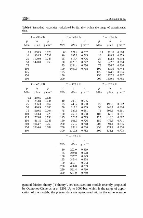
Table 4 presents the smoothed values forn-decane viscosity. The addeddensities have been taken from Gehrig and Lentz [9] using the Tait Equationof State.

In Table 5, the coefficients of the polynomial approximation (Eq. (5)) aregiven together with the mean average deviations between the experimental dataand the calculated curves. For an adequate reproduction of the data all digitsgiven in Table 5 have to be used.

Fig. 3 presents the viscosity as a function of temperature and pres-sure. The viscosity ofn-decane is much more pressure dependent than theviscosity of water. Ifη* denotes the relative viscosity at 323.2 K (η* =η(100 MPa)/η(0.1 MPa) the comparison shows:

η* (n-decane) = 2.44; η* (water) = 1.04.

The pressure dependence ofη* (n-decane) is, however, comparable with vis-cosities of other organic liquids, for example for benzene (2.22) and for iso-propanol (2.20). The isothermal density dependence of the viscosity is demon-strated in Fig. 4.

3.5 Comparison with literature data

Previously, the viscosity of liquidn-decane has been measured only withinmore limited ranges of temperature and pressure. Selected references are givenin Table 6.

Maximum and average deviations between literature data and the presentdata (Eq. (5)) are presented. Best agreement has been found with Krahnetal. [10] and Assaelet al. [11] with a maximum deviation not higher than 3%.The Carmichael data [12] have been used previously for the handbook on theviscosity of dense fluids by Stephan and Lucas [13]. Further data have beenmeasured by Leeet al. [14], Keramidi et al. [15], Tarzimanovet al. [16],Ducoulombieret al. [17], Oliveira et al. [18], Estrada-Baltazaret al. [19]. Inaddition, the present data are also in good agreement with the one-parameter


Table 4. Smoothed viscosities (calculated by Eq. (5)) within the range of experimentaldata.

T = 298.2 K T = 323.2 K T = 373.2 K

p η ρ p η ρ p η ρ

MPa µPa s g cm−3 MPa µPa s g cm−3 MPa µPa s g cm−3

0.1 860.5 0.726 0.1 621.2 0.707 0.1 371.0 0.66810 964.5 0.733 10 697.8 0.715 10 418.5 0.67925 1129.0 0.743 25 818.4 0.726 25 493.2 0.69450 1420.0 0.758 50 1029.9 0.742 50 622.7 0.71475 75 1254.4 0.756 75 756.7 0.730

100 100 1497.3 0.768 100 895.9 0.744125 125 125 1044.1 0.756150 150 150 1207.2 0.767200 200 200 1609.5 0.785

T = 423.2 K T = 473.2 K T = 523.2 K

p η ρ p η ρ p η ρ

MPa µPa s g cm−3 MPa µPa s g cm−3 MPa µPa s g cm−3

0.1 250.5 0.62810 283.8 0.644 10 208.3 0.60625 336.3 0.662 25 248.2 0.630 25 193.0 0.60250 426.9 0.686 50 317.3 0.659 50 248.7 0.63675 519.5 0.704 75 387.6 0.681 75 305.5 0.661

100 613.4 0.720 100 458.0 0.698 100 362.2 0.681125 709.8 0.733 125 528.7 0.713 125 418.6 0.697150 811.5 0.745 150 601.3 0.726 150 475.5 0.711200 1044.7 0.765 200 758.7 0.748 200 594.4 0.736250 1334.6 0.782 250 938.2 0.766 250 721.7 0.756300 300 1119.8 0.782 300 838.1 0.773

T = 573.2 K

p η ρ

MPa µPa s g cm−3

50 202.0 0.59975 249.8 0.628

100 297.7 0.649125 345.4 0.668150 393.1 0.683200 490.8 0.709250 591.4 0.730300 677.0 0.749

general friction theory (“f-theory”, see next section) models recently proposedby Quinones-Cisneroset al. [20]. Up to 1000 bar, which is the range of appli-cation of the models, the present data are reproduced within the same average


Table 5. Coefficients of polynomial fit Eq. (5). The maximum average deviation is< 0.46%, the mean average deviation is 0.11%.

a0 2.4369749706805E+02a1 −9.4864843755612E+01a2 +1.0748432202136E+01a4 −4.3045011897922E-02b1 +4.9942546669308E-02b2 +7.8396829767028E-04b3 +1.901980229E-07b4 −2.3409612297009E-10c1 −1.6136801775688E-02c2 +1.6633544715698E-03c3 −2.5441554206551E-04c4 +1.9023448171298E-05

Fig. 3. Viscosity of n-decane as a function of temperature and pressure. The diamondmarkers are the experimental data, the lines are calculated by Eq. (5).

deviation as reported forn-decane by Quinones-Cisneroset al. [21] between1.3% and 1.5%.

4. Discussion

4.1 Theoretical considerations

A number of efforts have been made to describe and calculate the viscosity ofnonpolar fluids for wide ranges of densities and temperatures. A satisfactoryrepresentation can be achieved with the “relative free volume concept” and the


Fig. 4. Viscosity ofn-decane as a function of density, above 1700×10−6 Pa s extrapolatedwith Eq. (5).

Table 6. References for comparison of data.

Authors Temperature Pressure Viscosity ViscosityRange Range Max. Dev. Av. Dev.

K MPa % %

Estrada-Baltazaret al. 1998 [19] 298−373 0.1−24.6 6.2 1.4Krahnet al. 1994 [10] 298−473 0.1−200 2.8 0.7Assaelet al. 1992 [11] 303−323 0.1−63.7 3.1 0.6Oliveira et al. 1992 [18] 303−348 0.1−254 11.3 1.7Ducoulombieret al. 1986 [17] 293−373 0.1−100 7.3 2.2Tarzimanovet al. 1986 [16] 298−373 1.01−98 15.0 3.7Keramidi et al. 1974 [15] 302−481 0.1−49 5.1 1.5Carmichaelet al. 1969 [12] 277−477 0.1−36 10.7 1.9Leeet al. 1965 [14] 311−511 1.4−55.2 12.4 2.6

viscosity correlation of Dymondet al. [22, 23]. The procedure can be comparedwith a Tait Equation approach.

For an accurate and convincing viscosity modeling covering the entire tem-perature and pressure range of the reported data, the “f-theory” suggested byQuinones-Cisneroset al. [21] can be used along with a cubic equation ofstate (EOS), e.g. the Peng-Robinson (PR) or the Soave-Redlich-Kwong (SRK)equations. In the f-theory, the viscosityη is separated into two parts, a “dilute-gas-term”η0 and a “friction term”ηf Eq. (7).

η = η0 +ηf . (6)


Table 7. Numerical values for the constants in the 8-parameters model Eq. (8).

u1 1.83429µPa su2 1.56659µPa su3 −0.887914µPa sv1 −2.62104µPa sv2 1.74523µPa sv3 −0.686084µPa sw2 −0.00025507µPa sw3 0.000375263µPa s

For n-decane, the dilute gas termη0 can be calculated using the equationsuggested by Chunget al. [24]. The friction term,ηf , is given by Eq. (7)

ηf = κr

pr

pc

+κrr

(pr

pc

)2

+κa

pa

pc

(7)

wherepr and pa are the Van der Waals repulsive and attractive pressure termsand pc the critical pressure. The friction parametersκr, κa, andκrr are given bythe following parametric model in Eq. (8):

κr = u1 exp[T−1

r −1]+u2

{exp

[2(T−1

r −1)]−1

}+u3

{exp

[3(T−1

r −1)]−1

}κa = v1 exp

[T

−1

r−1

]+v2

{exp

[2(T

−1

r−1

)]−1}+v

3

{exp

[3(T

−1

r−1

)]−1}

κrr = w2

{exp

[2T

−1

r

]−1}+w

3

{exp

[3T

−1

r

]−1}. (8)

This model is an extension of the 5-parameters model proposed byQuinones-Cisneroset al. to an 8-parameters model [21]. This has been done inorder to improve modelling in the complete temperature range of the presentmeasurements. The additional 3 parameters account for a third order tem-perature extension of the original model, which was only a second orderexponential model in temperature. For the estimation of the 8 parametersin Eq. (8) the model was least squares (LS) fitted against the experimen-tal data (Table 2). The equation of state used in the calculations was thePR EOS. The critical pressure, temperature, and acentric value required forthe PR EOS, as well as the critical volume required in the dilute gas vis-cosity model were all taken from Reidet al. [25]. The numerical valuesfor the constants in the friction parameters are given in Table 7. The erroranalysis of the derived model results in an absolute average deviation of0.83% with a maximum deviation of 4.28% (over prediction) at 470.1 Kand 20 MPa.

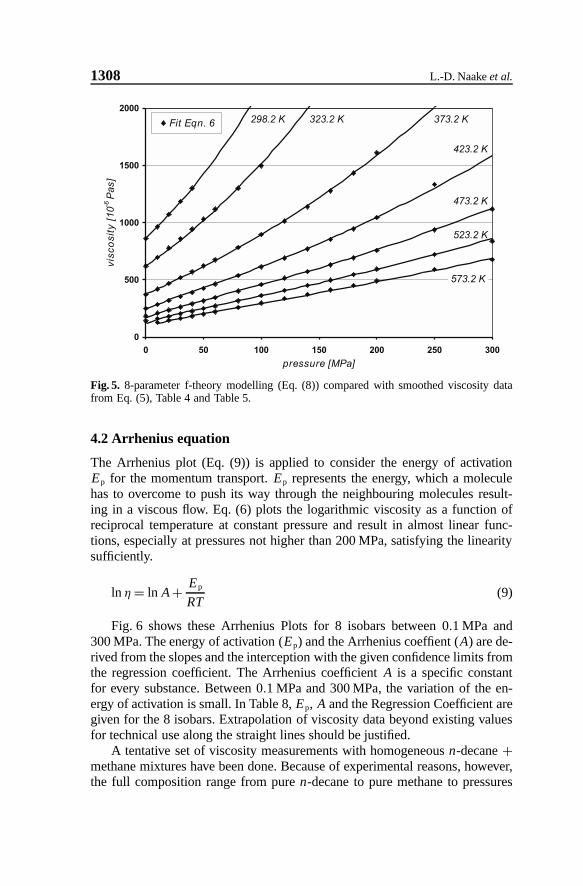
Fig. 5 shows the viscosityvs. pressure diagram obtained with the f-theorymodel for 7 isotherms covering the entire temperature and pressure range of thedata. For the low temperature isotherms (e.g. 373 K) the calculations have beenextended up to 300 MPa showing the stability of the model under extrapolation.


0

500

1000

1500

2000

0 50 100 150 200 250 300

Fig. 5. 8-parameter f-theory modelling (Eq. (8)) compared with smoothed viscosity datafrom Eq. (5), Table 4 and Table 5.

4.2 Arrhenius equation

The Arrhenius plot (Eq. (9)) is applied to consider the energy of activationEp for the momentum transport.Ep represents the energy, which a moleculehas to overcome to push its way through the neighbouring molecules result-ing in a viscous flow. Eq. (6) plots the logarithmic viscosity as a function ofreciprocal temperature at constant pressure and result in almost linear func-tions, especially at pressures not higher than 200 MPa, satisfying the linearitysufficiently.

ln η = ln A+ Ep

RT(9)

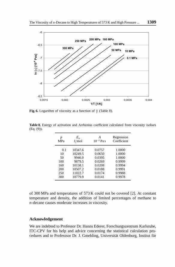
Fig. 6 shows these Arrhenius Plots for 8 isobars between 0.1 MPa and300 MPa. The energy of activation (Ep) and the Arrhenius coeffient (A) are de-rived from the slopes and the interception with the given confidence limits fromthe regression coefficient. The Arrhenius coefficientA is a specific constantfor every substance. Between 0.1 MPa and 300 MPa, the variation of the en-ergy of activation is small. In Table 8,Ep, A and the Regression Coefficient aregiven for the 8 isobars. Extrapolation of viscosity data beyond existing valuesfor technical use along the straight lines should be justified.

A tentative set of viscosity measurements with homogeneousn-decane+methane mixtures have been done. Because of experimental reasons, however,the full composition range from puren-decane to pure methane to pressures


Fig. 6. Logarithm of viscosity as a function of1T

(Table 8).

Table 8. Energy of activation and Arrhenius coefficient calculated from viscosity isobars(Eq. (9)).

p Ep A RegressionMPa J/mol 10−6 Pa s Coefficient

0.1 10347.6 0.0757 1.000010 10249.5 0.0650 1.000050 9946.0 0.0395 1.0000

100 9879.5 0.0269 0.9999160 10158.1 0.0208 0.9994200 10507.2 0.0188 0.9991250 11022.7 0.0174 0.9988300 10779.9 0.0141 0.9978

of 300 MPa and temperatures of 573 K could not be covered [2]. At constanttemperature and density, the addition of limited percentages of methane ton-decane causes moderate increases in viscosity.

Acknowledgement

We are indebted to Professor Dr. Hanns Ederer, Forschungszentrum Karlsruhe,ITC-CPV for his help and advice concerning the statistical calculation pro-cedures and to Professsor Dr. J. Gmehling, Universität Oldenburg, Institut für


Technische Chemie for a set of reference data onn-decane viscosity. AssociateProfessor Dr. Sergio E. Quiñones-Cisneros, Technical University of Denmark,Lyngby, Department of Chemical Engineering, provided the f-theory data. Wethank Professor Dr. E. Dinjus for the possiblity to use the facilities of the ITCInstitute at Forschungszentrum Karlsuhe.

References

1. W. Wakeham, A. Nagashima, and J. Sengers, IUPAC Physical Division, Commis-sion of Thermodynamics 3 (1991).

2. L.-D. Naake,Die Viskosität von N-Dekan und Methan-Dekan-Mischungen bis300◦C und 3000 Bar, PhD thesis, Universität Karlsruhe (1984).

3. O. Meyer, Wied. Ann. Phys.32 (1887) 642.4. E. Vogel, Wiss. Z. Universität Rostock18 (1969) 887.5. G. Macwood, Physica5 (1938) 374.6. G. Macwood, Physica5 (1938) 763.7. J. Kestin and I. Shankland, J. Appl. Math. Phys.32 (1981) 533.8. J. Kestin and I. Shankland, J. Non-Equilibr. Thermodyn.6 (1981) 241.9. M. Gehrig and H. Lentz, J. Chem. Thermodyn.15 (1983) 1159.

10. U. Krahn and G. Luft, J. Chem. Eng. Data39 (1994) 670–672.11. M. Assael, J. Dymond, and M. Papadaki, Fluid Phase Equilibria75 (1992) 287–290.12. L. Carmichael, V. Berry, and B. Sage, J. Chem. Eng. Data14 (1969) 27.13. K. Stephan and K. Lucas,Viscosity of dense fluids, Plenum Press (1979).14. A. Lee and R. Ellington, J. Chem. Eng. Data10 (1965) 346–348.15. A. Keramidi, Y. Rastorguev, M. Assael, and B. Grigoryev,Materialy Vsesoyuznogo

Soveshchaniya Po Fizike Zhidkostei7 (1974) 221–227.16. A. Tarzimanov, V. Arslanov, and R. Diveev,Termodyn. I Teplofiz. Svoistva Veshch-

estv. Sbornik Nauchn. Tr. Moskvov114 (1986) 51–57.17. D. Ducoulombier, H. Zhou, C. Boned, J. Peyrelasse, H. Saint-Guirons, and P. Xans,

J. Phys. Chem.90 (1986) 1692–1700.18. C. Oliveira and W. Wakeham, Int. J. Thermophys.13 (1992) 773–790.19. A. Estrada-Baltazar, J. Alvarado, and G. Iglesias-Silva, J. Chem. Eng. Data43

(1998) 441–446.20. S. E. Quinones-Cisneros, C. K. Zeberg-Mikkelsen, and E. H. Stenby, Fluid Phase

Equilib. 178 (2001) 1.21. S. E. Quinones-Cisneros, C. K. Zeberg-Mikkelsen, and E. H. Stenby, Fluid Phase

Equilib. 169 (2000) 249.22. J. Dymond, K. Young, and J. Isdale, Int. J. Thermophys.1 (1980) 331–343.23. J. Dymond, J. Robertson, and J. Isdale, Int. J. Thermophysics2 (1981) 133–154.24. T.-H. Chung, M. Ajlan, L. L. Lee, and K. E. Starling, Ind. Eng. Chem. Res27

(1987) 671.25. R. C. Reid, J. M. Prausnitz, and B. E. Poling, McGraw-Hill Book Company: New

York 4 (1987).26. D. Rathmann, J. Bauer, and P. Thompson, Bericht des Max-Planck-Institutes fuer

Stroemungsforschung6 (1978) 77.

the viscosity of n-decane to high temperatures of 573 k and high pressures of 300 mpa

Documents