the variation of capitalization rates across submarkets

1

The Variation of Capitalization Rates across Submarkets within the Same Metropolitan Area

by

Yisheng Yu

B.S. Architecture, 1994 QingDao Institute of Architecture and Engineering

Submitted to the Department of Urban Studies and Planning on August 5, 2004

in partial fulfillment of the Requirement for the Degree of Master of Science in Real Estate Development

at the

Massachusetts Institute of Technology

September 2004

@ 2004 Yisheng Yu All rights reserved

The author hereby grants to MIT permission to reproduce and to distribute

publicly paper and electronic copies of this thesis document in whole or in part Signature of Author

Department of Urban Studies and Planning August 05, 2004

Certified by

William C. Wheaton Professor of Economics

Thesis Supervisor Accepted by

David M. Geltner Chairman, Interdepartmental Degree Program

in Real Estate Development

2

The Variation of Capitalization Rates across Submarkets within the Same Metropolitan Area

by

Yisheng Yu

Submitted to the Department of Urban Studies and Planning on August 5, 2004

in partial fulfillment of the Requirement for the Degree of Master of Science in Real Estate Development

ABSTRACT This paper investigates the variation of capitalization rates across submarkets within the

same metropolitan area by using a database with 73 transactions of office properties

located in nine submarkets of Atlanta during the period from the third quarter of 2000 to

the second quarter of 2003. The results show that capitalization rates are quite

predictable at the submarket level. Movements of capitalization rates are shaped by local

market information, national capital market information and characteristics of individual

property. The study also examines the behavior of real estate investors in forming their

expectations of future income streams. A cross-sectional model with time dummy

variables is used in this paper.

Thesis Supervisor: William C. Wheaton Title: Professor of Economics

3

ACKNOWLEDGEMENTS

Special thanks first go to my supervisor Professor Wheaton for his guidance and

generous support in these two months. I feel very privileged to have had an opportunity

to study under him. His insight, wisdom and encouragement allow me to shape and

complete my research, and also to develop confidence for my future career.

Special thanks are also offered to Hines and Torto Wheaton Research, and in particular,

Blake Williams from Hines Capital Markets Group in Houston, Jacob Vallo from Hines

in the Atlanta office, and James Costello from Torto Wheaton Research in Boston. In

addition, I highly appreciate Dave Mahoney from Merrill Lynch & Co., Inc, New York,

who provided his insight and suggestion in shaping and developing my thesis. This paper

would not have been possible without their support.

I would like to thank my two friends, Victor Chen and Christopher Braswell. Both of

them gave me significant help to complete this paper perfectly.

Finally, this thesis is dedicated to my wife, Yiwei, and my parents. Their sacrifices and

unwavering support throughout this disruptive year have made my educational

experience at MIT all the more enriching.

4

TABLE OF CONTENTS

ABSTRACT

ACKNOWLEDGEMENTS

CHAPTER 1: INTRODUCTION 1.1 Background………………………………………………………......................... 6

1.2 Roles of Capitalization rates……………………………………………………... 6

1.3 Objectives and Findings………………………………………………………….. 7

CHAPTER 2: EMPIRICAL WORK 2.1 Capitalization Rates in a Global Context……………………………………….. 9

2.2 Capitalization Rates Linked to National Markets……………………………… 10

2.3 Capitalization Rates on Local Market Scale…………………………………… 10

2.4 Market Context This Paper Focus on…………………………………………... 12

CHAPTER 3: METHODOLOGY 3.1 Capitalization Rates in Efficient and Equilibrium Market…………………….. 13

3.2 Decomposition of Capitalization Rate…………………………………………. 14

3.2.1 Risk-free Rate………………………………………………………………….. 15

3.2.2 Risk Premium…………………………………………………………………. 15

3.2.3 Expected Rental Growth Rate………………………………………………… 16

CHAPTER 4: DATA and ESTIMATION 4.1 Overview………………………………………………………………………. 18

4.2 Transaction-based Properties………………………………………………….. 18

4.2.1 Estimation of Operating Costs………………………………………………… 19

4.2.2 Transaction-based Capitalization Rates……………………………………….. 21

4.2.3 Data Descriptions of Transaction Properties…………………………………... 22

4.3 Submarkets Information Data………………………………………………….. 25

CHAPTER 5: MODELING FRAMEWORK 5.1 Overview………………………………………………………………………… 27

5.2 Characteristics of Individual Property…………………………………………... 27

5

5.3 Local Submarket Factors………………………………………………………... 28

5.3.1 Local-fixed Factors……………………………………………………………... 28

5.3.2 Correlation Analysis for Local-fixed Factors…………………………………....33

5.4 National Capital-market Factors and Other Time-variant Factors………………. 35

5.4.1 National Capital-market Factors…………………………………………………35

5.4.2 Other Time-variant Factors……………………………………………………... 36

5.5 Model …………………………………………………………………………….36

CHAPTER 6: ESTIMATION RESULTS 6.1 Characteristics of Property………………………………………………………... 37

6.2 Local Market Factors……………………………………………………………… 38

6.3 Time Dummy Variables……………………………………………………………41

6.4 Summary……………………………………………………………………………42

CHAPTER 7: CONCLUSION 7.1 Findings…………………………………………………………………………… 44

7.2 Further Research...……………………………………………………………….... 45

REFERENCES

CHARTS

6

CHAPTER 1 - INTRODUCTION

1.1 Background

In real estate, the capitalization rate is traditionally used to capture the relationship

between the current net operating income and property value. It measures the ability of a

property to generate future incomes after deducting from operating expenses and normal

vacancy but before deducting financing charges and income taxes. The capitalization rate

is very closely related to the overall return of a property before financing and taxes, and it

is used worldwide.

1.2 Roles of Capitalization Rates

To further recognize the important role of the capitalization rate in real estate, three major

fields that heavily rely on the capitalization rate need to be specified. First of all, the

capitalization rate plays a particularly important role in property valuation for real estate

investors. Compared to the discount cash flow (DCF) valuation model, discounting the

forecasted cash flows by explicating the appropriate risk and return factors of the

investment, the capitalization rate looks more like a short-cut and does not completely

represent the overall return of a property. As a comparable measure, however, it actually

reflects the investors’ perceptions of risk and expectations of returns by converting the

market expected income stream from a commercial property into an estimate of asset

market value by dividing the net operating income stream by the expected capitalization

rate (Brueggeman and Fisher, 1993).

7

Secondly, market analysts use the capitalization rate as a very good measure to interpret

the real estate market development. Fundamentally, the capitalization rate should reflect

the information driven from real estate space market. On the other hand, the real estate

market, as an asset market, should be integrated into the whole capital market due to the

competitive national capital market. The capitalization rate representing investors’

perceptions of risk and expectations of returns is comparable to some financial

parameters, such as corporate P/E ratio, interest rate, and S&P 500 index. Thus,

movements of capitalization rates provide a good index to track the development of the

real estate market by shedding the light on the link between real estate space market and

national capital asset market.

Finally, the academics often apply the capitalization rate to test for market efficiency,

especially for the private real estate market. The capitalization rate reflects heterogeneous

investors’ expected returns across different local real estate markets, which usually have

different amounts of inherent investment risk. Due to the degree of market information

efficiency, investors might have different perceptions of risk for the local markets with

the same profile of risk, and meanwhile the impacts on capitalization rates from space

markets may be lagged. Many academics have researched and are working on such

studies about the segments of the real estate market by analyzing capitalization rates

across different markets.

1.3 Objectives and Findings

8

Motivated by the importance of the capitalization rate, this paper attempts to explore the

variation of capitalization rates across submarkets within the same metropolitan area. The

study examines seventy-three transacted properties across nine submarkets in Atlanta

during the period from the third quarter of 2000 to the second quarter of 2003, when

market rents and the interest rate dropped dramatically. The data includes characteristics

of properties such as ages and floors, and submarket information such as market size,

annual absorption and completion, vacancy rate, and rental growth.

The results of this paper show that capitalization rates are strongly predictable at the

submarket level. Characteristics of property, such as age and floor, are very important

determinants of the capitalization rate by affecting investors’ perceptions of risk and

expectations of rental income. Movements of market-specific capitalization rates exhibit

a high incorporation with the national capital market, as well as with local office-market

features, including space stock level, absorption rate, and past rate of rental income

growth. The study also discusses whether real estate investors use a ‘backward-looking’

approach or a ‘forward-looking’ in forming their expectations of future incomes.

The rest of this paper is structured as follows. First, it reviews some empirical work on

capitalization rates, and then states methodology in the third section. The fourth section

describes data and some estimations, while laying out the modeling frame work in the

fifth section. The estimation results appear in the sixth section. A final conclusion and

future desirable research are discussed in the seventh section. The references are attached

on the last pages.

9

CHAPTER 2 – EMPIRICAL WORK

As the capitalization rate is such a valuable measure in estimating property valuation,

interpreting real estate market development and testing for market efficiency, it is not

surprising that there are such extensive empirical studies on the capitalization rate (or

return). The research can generally be separated into three main camps in terms of the

different market contexts they focus on.

2.1 Capitalization Rates in a Global Context

First of all, some research study capitalization rates in a global context. The recent papers

include: Case et al. (1999) examine the impact of changes in GDP on property returns.

They find that the international GDP and country-specific GDP have the explaining

power for movements of indirect real estate returns. Ling and Naranjo (2000) perform a

cross-country analysis on indirect real estate returns. They report that country-specific

effects drive indirect real estate returns. Eichholtz and Huisman (1999) investigate the

cross section differences between expected excess returns on the international shares. The

results show that market size and interest rates have important influences on excess

property share returns. Wit and Dijk (2003) examine the determinants of direct office real

estate returns by analyzing a global database across Asia, Europe, and the United States.

They find that gross domestic product, inflation, unemployment, vacancy rate, and the

available stock all have an impact on real estate returns.

2.2 Capitalization Rates Linked to National Market

10

The second camp of the empirical literatures investigates the variation of capitalization

rates by linking it to national economic variables. For examples, Fisher, Lentz and Stern

(1984) and Nourse (1987) explore the relation between capitalization rates and tax

regimes by using data from the American Council on Life Insurance (ACLI). They report

changes of capitalization rates when real estate related tax law changed. Froland (1987)

looks at impacts on capitalization rates from the competitive asset trading market, using

quarterly capitalization rates for apartments, retail, office, and industrial property from

the first quarter of 1970 through the second quarter of 1986. He finds particularly strong

correlations of capitalization rates with mortgage rates, ten-year bond rates, and corporate

P/E ratio. Chandrashekaran and Young (2000) create a sector model and then used it to

its predictive power when they find interactions between capitalization rates and S&P

500, inflation measures and inflation and default spreads. It is worth to note that these

studies above usually only involve the time-series movements of capitalization rates

without cross-section variants.

2.3 Capitalization Rates on Local Market Scale

Some research study that local real estate market information should have strong effects

in shaping capitalization rates. In these studies, the authors usually apply the cross-

sectional analysis method to explore the variation of capitalization rates across broad

property types or different metropolitan areas. Ambrose and Nourse (1993) use data from

the American Council of Life Insurance (ACLI), and find the regional variation of

capitalization rates by defining some national real estate market areas as North, South,

East and West. Jud and Winkler (1995) draw other financial theoretical under-pricings of

11

the WACC and CAPM models to develop a theoretic model of the capitalization rate for

real estate properties. By using the National Real Estate Index panel database of twenty

one metropolitan areas for fifteen half-year periods starting in the second half of 1985,

they find that movements of capitalization rates are strongly related to changes in capital

market returns, but the adjustments have significant lags and market relationships vary

across local areas. Sivitanidou and Sivitanidies (1999) look at metropolitan-specific

office capitalization rates and report serial correlation in area-specific time trends, by

using a panel approach to analyze office market capitalization rates in seventeen

metropolitan areas over the period of 1985-95. Sivitanides, Jon Southard, Torto and

Wheaton (2001) apply a panel approach to study how capitalization rates vary across

metropolitan markets and time by systematically examining NCREIF data. The database

includes data across fourteen metropolitan areas for sixteen years starting in 1983. They

report that local market factors play an extremely important role in the variation of

capitalization rates, and that appraisal-based valuation is more “backward” than

“forward” looking.

With studies of the third camp, people realized that the real estate market is segmented in

some aspects, particularly in the boundary of metropolitan areas. However, there are very

little studies to explore the spatial differences in capitalization rates on individual

properties, especially across submarkets within the same metropolitan area. The reason

might be the lack of data of individual property cross-sections or time series. Some recent

exceptions are: Hendershott and Turner (1999) and Janssen, Soderberg and Zhou (2001)

do research in individual property context, by both using 403 property transaction-based

12

capitalization rates in Stochholm from the second quarter of 1990 to the second quarter of

1992. Hendershott and Turner calculate ‘constant-quality’ capitalization rates across three

property types and five semiannual periods , by using variables including density of land

use, building age, property type, a measure of below-market financing and time dummy

variables. They uncover that building quality adjustment and property types are very

important in determining capitalization rates. This paper also reports a location factor by

using location dummy variables. Janssen, Soderberg and Zhou use hedonic models to

explain capitalization rates across building types, ages and four specific locations. They

find that capitalization rates significantly depend on property features. Clayton, Geltner

and Hamilton (2001) study 202 appraisals on 33 properties in Canada over the period of

1986-96. Rather than the issue of cross-sectional determinants of valuations, they are

more concerned with the smoothing issues of time-series appraisal.

2.4. Market Context This Paper Focuses On

Against the background that there are rare studies investigating the capitalization rate in

the submarket context, this paper will explore the variation of capitalization rates across

nine submarkets within the Atlanta metropolitan area by using seventy-three office

property transaction-based data and a cross-sectional analysis approach. The results show

that characteristics of properties, submarket real estate information, and national capital

market have strong influences on capitalization rates.

13

CHAPTER 3 - METHODOLOGY

3.1 Capitalization Rates in Efficient and Equilibrium Market

As mentioned before, the capitalization rate is the ratio of future net operating income

(NOI) to property value. The property value here should be determined by the interplay

between the demands from asset market and the supply from space market. If the market

is perfectly efficient and competitive enough, the property value should be the transaction

price, as well as the present value of the future net income the property is expected to

generate. In other words, the capitalization rate can be depicted as

Cap rate = NOI1 / PV (of property) (1)

PV (of property) = NOI1/ (1+i) + NOI2/ (1+i) 2 + ... +NOI t/ (1+i) t (2)

To simplify, Formula (2) assumes that the discount rate (i) keeps constant during the

property expected holding period. For the theory of market efficiency, (i) represents the

minimum required rate of return for marginal investors. It should and must reflect the

appropriate risk of expected cash flow. The future income stream would not change if the

space market is in equilibrium. The equilibrium is explained by the combination that the

vacancy rate is equal to a natural vacancy rate and that the expected rental growth is the

same as the depreciation rate forever (Hendershott and Turner (1999)). In addition, if the

investors do not change their perception of risk, the property value would not change

either. Thus, in such an ideal environment, the capitalization rate would not change.

14

Of course, markets are not always in equilibrium. Empirical evidence has shown that the

property space market seems to exhibit periodic movements of overbuilding and under-

building where vacancy rates and rent deviate significantly from equilibrium values.

Furthermore, the space market and even the capital market are not completely efficient.

The interplay between the asset market and the space market is not non-friction. The

heterogeneous investors would have different perceptions of risk and these perceptions

vary by time. These factors cause movements of property values, especially in

heterogeneous markets. Empirically, values and rents do not move one for one, and

theoretically we would expect values to move less cyclically than rents (Wheaton, 1998).

All of those result in the variation of capitalization rates across markets and time series.

3.2 Decomposition of Capitalization Rate

To better understand movements of capitalization rates, we will continue to decompose

the capitalization rate. If the future net income is expected to grow at a constant rate (g)

forever, NOIt = NOIt-1*(1+g), mathematically it is able to get a more simplified equation,

Cap rate = i – g. Moreover, the discount rate (i), which reflects both capital opportunity

costs and market risk, can be split into two other components, risk free rate (rf) and

appropriate risk premium (rp), respectively. Therefore we are able to express the

capitalization rate as

Cap rate = rf + rp – g (3)

15

3.2.1 Risk-free Rate

It seems to be obvious that the using of the risk free rate is a valuable measure of risk, as

all investors have to compete hard for capital in an ‘integrated’ national capital market.

The risk-free rate presents the time value of assets, and theoretically it reflects a

guaranteed return without any risk. Thus, it is reasonable that investors in real estate

expect a higher return, which results in a higher capitalization rate, in response to rises of

interest rate. Although the 10-year Treasury bill rate does not perfectly match the risk

free rate as the Treasury bill has default risk and there are different profiles of liquidity

risk between real estate assets and finance assets, Sivitanides, Jon Southard, Torto and

Wheaton (2001) have shown that the 10-year Treasury rate “worked better than other

masteries and is consistent with the conventional view of real estate as a long-term

investment vehicle”.

3.2.2 Risk Premium

The risk premium component is much more difficult to quantify than the risk free rate. In

finance, arbitrary portfolio theory (APT) proves that risk premium should include any

risk associated with individual property, and its return should be the rate of overall return

net the risk free rate.

Empirically, there are three main factors affecting the property risk premium. First,

national capital market information should have an impact on the risk premium

(Sivitanides, Jon Southard, Torto and Wheaton (2001)). When interest rate rises, it not

only adjusts the risk free rate mentioned above, but also changes risk perspectives of

16

investors. They might ask more or less price for a ‘unit’ of risk. Second, local market

factors should matter as well (Sivitanidou and Sivitanidies (1999), and Grissom, Hartzell

and Liu (1987)). Risk perceptions should be shaped by some specific structural features

of the metropolitan area or of its submarkets. Those features include market size,

vacancy level, annual absorption and completion, employment, GMP, and so on. Third,

characteristics of the property, such as age, floor, location, and density of land use, are

most likely to influence the investors’ perceptions of risk (Hendershott and Turner

(1999)) and expectations of rental growth. A building with a superior location might be

less risky for investors than a building in an inferior area in generating a future income

stream if all other variables are held constant.

3.2.3 Expected Rental Growth Rate

If we split the expected rate of rental growth into the expected rate of real rental growth

and expected general inflation growth rate, it would be relatively easier to clarify the

factors driving expectation of income growth. As a national economic factor, the

expected general inflation rate should have an impact on the capitalization rate. When the

inflation rate is predicted to be higher, real estate investors will expect a higher growth

rate in rental income. They would like to pay a higher price to acquire the property now

and accept a lower capitalization rate.

In real estate, the estimation of the growth rate of future income is usually based on

market rents, as the existing lease structure often causes significant lags between changes

in market rent and changes in property income. Thus, the expected rate of real rental

17

growth is replaceable by the expected growth rate of real market rent, which is largely

determined by the level of expected local space market demand and supply. At the

submarkets level, the demand and supply of space market is mainly reflected by vacancy

rate and annual absorption and completion rates. Furthermore, the characteristics of

property might affect the future growth rate of rental income as well. The buildings with

different ages could have different expected rental growth rates because of their different

abilities to generate future cash flows and their different expected obsolescence rates.

To further understand the expected growth rate of real market rent, however, it is very

important to know another theory about the movements of the real estate market.

Wheaton (1998) points out that real estate markets always exhibit periodic episodes of

under-building and over-building, suggesting that prices or rents are typically mean-

reverting, stationary series. The property markets are not random walks, and movements

of markets are quite predictable. This theory provides a good judgment of whether the

market expectation is ‘forward-looking’ or ‘backward-looking’, which reflect the degree

of efficiency for real estate markets. When the market rent is at or near historic highs,

rational investors should anticipate a lower subsequent income growth when they use the

‘forward-looking’. If the market rent is near a historic low, the rational investors should

have a higher growth expectation. On the other hand, if the investors like to use the

‘backward-looking’ method, they would have opposite expectations when the rent is at

historic highs or lows. That is, when the market is up, they will assume that this growth

will continue even further and have a higher expected growth rate than the rational

investors have.

18

CHAPTER 4 - DATA AND ESTIMATIONS

4.1 Overview

The data is supplied by Real Capital Analytics (RCA) and Torto Wheaton Research

(TWR), two well-known companies in producing a national real estate market database.

RCA provided the raw data that records seventy-three office property transactions during

the period from the third quarter of 2000 to the second quarter of 2003 in Atlanta. TWR

combined the RCA’s raw data with its own database, especially in rental income.

Meanwhile, TWR provided the historic information of nine submarkets, where the

seventy-three properties are located, from the fourth quarter of 1987 to the first quarter of

2004 in Atlanta.

4.2 Transaction-based Properties

Among the raw data of seventy-three transactions, every property records its transaction

price and some physical characteristics, such as total floor area, floors, built year, and

location (zip code). All properties have rarely good capitalization rates except seventeen

properties. To measure the capitalization rate for an individual property, we have to

estimate its rental income stream, which RCA does not provide. TWR uses a two-part

process to estimate an appropriate market gross rental income stream for every individual

property. First, if the asset in question could be matched directly between the two

databases, TWR uses market asking rent and occupancy history for the tracked building

to estimate a gross "income" series. The rents were grossed up when they are quoted on a

net basis and represented "income" as it showed the asking rents without any

19

concessions. Combining assumptions on a typical 5 year-lease term with the rent and

occupancy histories for the assets, TWR estimated these gross income streams for the

matched assets. Second, for those assets that could not be matched directly, TWR applies

the rents and occupancies of assets with similar physical characteristics in the location to

estimate those properties1.

Moreover, TWR made some estimations for built years as RCA reports the built years of

some properties in decades, such as 1960’s or 1970’s. The process of this estimation is

very similar to the way TWR estimated the income streams. TWR tried to match the

buildings to its own database to get the exact years first. There are seventeen properties in

this case that could not be matched. TWR estimated their built years by looking at what

sort of rents and occupancy a 1960's era building in that location, size and floor range.

4.2.1 Estimation of Operating Costs

To calculate the net capitalization rate, we still need to obtain an operating cost of every

property, which the database does not provide. Fortunately, there are seventeen properties

with their own closed capitalization rates, respectively. Thus, it is reasonable to utilize

these seventeen properties and build a model to estimate the operating costs of other

properties. As we all know,

Cap rate = (Occupancy rate *Gross rent – Operating cost) / Price (4)

1. For more details about TWR database and income stream estimation, please see Wheaton, Torto, Southard (1997) the Journal of Real Estate Literature, Vol. 5, 59-66, and visit the website www.tortowheatonresearch.com.

20

Equation (4) assumes that the total floor area is equal to the net rentable area as there is

no such information in this case. Every item on the right side of the formula should be in

dollars per square foot, expect occupancy rate as a percentage. Thus Equation (4) can be

derived as

Operating cost = Occupancy rate * Gross rent – Cap rate * Price (5)

Since most investors would like to use the expected average market vacancy rate instead

of the current vacancy rates of individual properties while valuing future income streams

of properties 2, plus in Atlanta this number tends to be 90%, this paper uses 90% as the

occupancy rates in Formula (5). Under this assumption, we can have a series of operating

costs of properties by utilizing the seventeen properties with closed capitalization rates.

On the other hand, the operating cost is very closely related to some characteristics of

individual property such as size, floor, and age. A high-rise that is an older building is

more likely to have a higher operating cost than a low-rise that is a brand new building.

In this case, the correlation between floor and size is relatively high (0.58). The building

size and age are used as two variables to build a hedonic model with the dependent

variable of the operating cost. The model is written as

Operating cost = f (size, age) (6)

2. Actual building occupancy rates and current vacancy rates of submarkets were also used to estimate the

operating costs. Neither of them had a better regression result than the one with 90% vacancy rate.

21

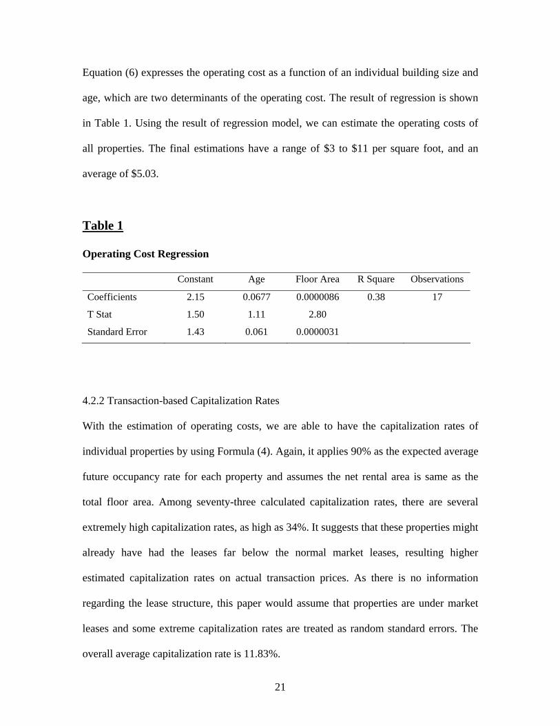
Equation (6) expresses the operating cost as a function of an individual building size and

age, which are two determinants of the operating cost. The result of regression is shown

in Table 1. Using the result of regression model, we can estimate the operating costs of

all properties. The final estimations have a range of $3 to $11 per square foot, and an

average of $5.03.

Table 1

Operating Cost Regression

Constant Age Floor Area R Square Observations

Coefficients 2.15 0.0677 0.0000086 0.38 17

T Stat 1.50 1.11 2.80

Standard Error 1.43 0.061 0.0000031

4.2.2 Transaction-based Capitalization Rates

With the estimation of operating costs, we are able to have the capitalization rates of

individual properties by using Formula (4). Again, it applies 90% as the expected average

future occupancy rate for each property and assumes the net rental area is same as the

total floor area. Among seventy-three calculated capitalization rates, there are several

extremely high capitalization rates, as high as 34%. It suggests that these properties might

already have had the leases far below the normal market leases, resulting higher

estimated capitalization rates on actual transaction prices. As there is no information

regarding the lease structure, this paper would assume that properties are under market

leases and some extreme capitalization rates are treated as random standard errors. The

overall average capitalization rate is 11.83%.

22

4.2.3 Data Descriptions of Transaction Properties

Tables 2, 3, 4, 5 (shown below) describe the data of seventy-three transacted properties in

terms of geography, deal time, property age and floors, respectively. The latter two

represent the characteristics of property.

Table 2 delineates the individual properties diversified by nine submarkets and the

number of transactions, average capitalization rates, average rents and transaction prices.

As can be seen, the average capitalization rates are quite different across the nine

submarkets. The lowest one is 6.77% in Buckhead, and the highest one is 15.26% in

Northeast Atlanta. Meanwhile, the lowest rents are around $16.5-$17.00 in Downtown

Atlanta, Midtown Atlanta and South Atlanta, while the highest average transaction price

is in Buckhead, $175.97. This information tells us that the average capitalization rate

could vary by the submarkets, but the variation is not only determined by the differences

of markets.

Table 3 depicts the number of property transactions according to four time periods, and

their average capitalization rates, rents and transaction prices. We can see that the

average capitalization rate increased in 2001, decreased in 2002 and rebounded in 2003.

The rents increased in 2001 and after that decreased continuously. The average prices

moved in the opposite way of the movements of the average capitalization rates,

decreasing in 2001, increasing in 2002 and deceasing in 2003 again. This table gives us

some sense of the movements of the average capitalization rates during four annual

periods from 2000 to 2003.

23

Table 4 and Table 5 show data descriptions by the property characteristics. Table 4

diversifies the properties by their ages. The average rent decreases as the building age

increases. However, the average capitalization rate increases as the building age

increases, except the properties with higher ages than 25. The mathematic reason is that

the average prices decrease more quickly than the average rents do when the properties

are younger than 25. The average prices decrease by 14% and the average rents decrease

by only 4%, when the ages of properties increase from below 5 to the range of 5-15. To

some extent, we might be able to conclude that the ages might have a positive impact on

the average capitalization rates, except for the buildings older than 25.

Table 5 describes the data by the floors of buildings. 59 out of 73 properties in the

database are 1-10 stories. The average capitalization rates decrease when the buildings

are higher. Neither the average rents nor the average prices move in the same way as the

capitalization rates. Compared to the changes in rents and prices by age (see Table 4), the

changes in rents and prices by floors are quite smooth. More importantly, when the

properties have less than 3 floors, the average capitalization rate is extremely high,

15.63%, almost 50% more than the average capitalization rate of properties with 5-10

floors. This might tell us that the investors view office properties with 1-2 floors in

Atlanta as extremely risky assets. They would like to ask for higher capitalization rates

than they do for others.

24

Table 2

Regional Distribution of Properties Submarkets Number Average Cap* Average Rent* Average Price*

Buckhead 5 6.77% 20.63 175.97

Central Perimeter 9 13.31% 22.03 135.47

Downtown Atlanta 6 10.48% 16.47 76.87

Midtown Atlanta 5 7.38% 16.89 145.97

North Fulton 14 8.94% 18.24 138.53

Northeast Atlanta 9 15.26% 17.85 93.06

Northlake 1 13.53% 18.63 84.98

Northwest Atlanta 18 14.68% 20.21 105.90

South Atlanta 6 11.66% 16.96 98.54

Total 73

Table 3 Annual Distribution of Properties

Time period Number Average Cap* Average Rent* Average Price*

2000 21 8.99% 18.63 135.37

2001 26 13.91% 19.18 107.49

2002 20 11.68% 19.06 120.36

2003 6 13.26% 18.93 100.83

Total 73

Table 4

Properties Distribution by Age

Building Age Number Average Cap* Average Rent* Average Price*

<5.0 15 10.09% 20.44 146.53

5.0-15.0 19 12.50% 20.32 126.98

15.0-25.0 21 14.36% 18.89 99.78

>25.0 18 9.63% 16.40 107.97

Total 73

25

Table 5 Property Distribution by Floors

Floors Number Average Cap* Average Rent* Average Price*

<3 23 15.63% 17.72 92.53

3-10 36 10.31% 19.10 129.66

10-20 9 9.96% 21.09 142.18

>20 5 8.66% 19.91 114.81

Total 73

* Average Cap represents the average capitalization rate of properties. Average Rent and Average Price

here is in dollars per square foot. The rent is the property market rent estimated by TWR and the price

represents the transaction price.

4.3 Submarkets Information Data

The second part of the database consists of nine submarkets information in Atlanta. It

includes the information of space market supply and demand, such as space stock (net

rentable area), physical vacancy rate, and the levels of absorption and completion, and the

information of asking gross market nominal rent. TWR tracked them quarterly from 1987

to 2004. Charts 1, 2, 3 and 4 (attached in last pages) show quarterly net rentable areas, the

levels of absorptions and completions, vacancy rates and asking gross rents for the nine

submarkets in Atlanta from the first quarter of 1994 to the first quarter of 2004.

Chart 1 depicts the movements of net rentable areas of submarkets. Among those

markets, South Atlanta had the smallest space market while Center Perimeter had the

largest one. South Atlanta, Northlake and Downtown Atlanta had the lowest growth in

office spaces over the past 10 years, and North Fulton had the highest growth, which

means that North Fulton was a highly developing market.

26

In Chart 2, North Fulton had the biggest completion over the past 10 years, and it seems

to be a leading market in construction among the nine submarkets. South Atlanta had the

lowest completion. The level of completion for each market went up quickly after 1997.

That is, the new construction in Atlanta was very active after 1997. In Chart 3, the trends

of absorptions in North Fulton, Center Perimeter and Downtown Atlanta had the biggest

standard deviations over the past 10 years. The trends in Northlake and South Atlanta had

the lowest deviation. There was a big drop in absorption for each market in 2001. That is,

the rental space demand decreased dramatically after 2001.

Chart 4 reports the tendencies of asking gross rent over the past 10 years. It seems that

there was a rent peak between 2000 and 2001. Midtown Atlanta and South Atlanta had

the highest average rental growth rate over the past 10 years. Center Perimeter had a

negative growth rate from 1994 to 2004. North Fulton had the biggest increase before

2001, and after that it had the biggest downturn. Chart 5 shows the physical vacancy level

from 1994 to 2004. The vacancy rate for each market, except for Downtown Atlanta, was

relatively low during the period from 1996 to 1999 and then increased continuously.

Downtown Atlanta moved in the opposite direction compared to others. Its vacancy rate

was high from 1994 to 1999 while low from 2000 to 2004. Northlake had the lowest

average vacancy rate over the past 10 years. Center Perimeter had the biggest increase in

vacancy rate, while South Atlanta had the biggest downturn from 2001 to 2004.

27

CHAPTER 5 – MODELING FRAMEWORK

5.1 Overview

Based on the discussion in Section III and using the data described in Section IV, we can

start to set an appropriate model to examine the variation of capitalization rates across the

submarkets, and to discover specific factors that may determine the capitalization rates.

We have learned that characteristics of properties, local real estate information and

national capital markets, may have an impact on the capitalization rates of individual

properties by adjusting the risk perception or income-growth expectations in time paths,

or both. These factors will be built into the model, which is usually referred as the cross-

sectional model with time dummy variables.

5.2. Characteristics of Individual Property

Firstly, the capitalization rate can be expressed as a function of characteristics of property

for a given property with market rent lease structure at a point in time. That is,

Cap rate = f (age, floors, bltest) (7)

In Equation (7), ‘bltest’ is a dummy variable if the age of property is estimated by TWR

since the raw transaction data reports its age in decades like the 1970’s or 1960’s. There

are 17 properties with such estimated ages. Using Equation (7), it is possible to check the

effects on the capitalization rate from the characteristics of property. The capitalization

28

rates calculated here are usually called “constant-quality” capitalization rates 3. This

concept provides a good way to compare the capitalization rates of properties with

similar physical qualities in different markets, and makes us better understand other

influences on capitalization rates.

5.3 Local Submarket Factors

Equation (7) must be modified since the local real estate market information should have

an impact on the capitalization rates as well. These factors can be separated into two

categories. One category is local-fixed office-market influences. These influences are

time-invariant and include some features that are not completely fixed but change slowly

through time (Sivitanidou and Sivitanides (1999)). The second category is time-variant

local office-market influences.

5.3.1 Local-fixed Factors

For the local-fixed office-market influences, this paper uses as variables the size of

submarket (NRA), the average vacancy rates (VAC), the average absorption rate (ABS)and

completion rate (CPT), and the average growth rate of asking gross rent (GRT) over past

several years.

3. Hendershott and Turner (1999) defines the constant quality capitalization rate as “ similar properties

trading in a given location where the tenants and landlords have a given set of leasing and financing options

and where the extent of above or below market existing leases and above or below market financing does

not vary”.

29

NRA is depicted as the current rentable area of a submarket. As a measure of space stock,

it may reflect the perception of liquidity risk and expectation of rental growth rate. With a

larger market, real estate investors might view it as a more liquid market than the smaller

market. They may accept a lower capitalization rate for a larger market based on the

liquidity risk. On the other hand, the rental income in the larger market is expected to

grow slower than the one in the small market if other factors are the same for both

markets. This factor will result in a higher capitalization rate for the larger market.

Overall, the coefficient sign of NRA depends on the offset from both influences.

Most professionals would like to treat ABS and GRT, CPT and VAC as time-variant

factors on the capitalization rate. However, in this paper the data pool is so small and

limited over only four annual periods. It is better to treat these four factors as time-

invariant influences and then take time-variant effects of them as dummy variables along

with other time-variant variables. ABS tends to measure the demand side information of

submarkets by representing the average of absorption levels over past years. It is depicted

as the average of percentages of the annual absorptions over the current space stock. It is

expected to have a positive impact on the capitalization rate by reducing investors’

perceptions of risk and expectation of rental growth rates. The higher the average annual

absorption rate, the lower the risk of a future potential decrease in rents and asset values.

Reflecting the income-growth expectation for a submarket, GRT is depicted as the annual

compounded rental growth rate over past years. If the investors are ‘backward-looking’,

the average growth rate of asking gross rent should have a negative impact on the

30

capitalization rate, since a historic high of rental growth rate makes those investors have a

higher expected future rental growth and accept a lower current capitalization rate. If the

investors were ‘forward-looking’, they would have opposite expectations. The reason is

that they would expect a lower future growth rate and thus a higher capitalization rate,

when the current rental growth rate is historically high.

CPT measures newly built and market-available spaces over the past years. This is

typically lagging information owing to the characteristic of the real estate construction

process. It is calculated by averaging the percentages of annual completions over the

current space stock. As a supply measure, CPT is expected to have a negative impact on

the capitalization rate. The higher the average completion rate, the lower the expected

rental growth rate and the higher the risk of investment.

VAC is calculated by the average of percentages of annual occupied spaces to the current

space stocks over past years. It would reflect the softness of the office-space markets and

the net supply for next year if there is no more new completion. Compared to a market

with a lower average vacancy rate, the market with a higher one should be expected to

have a lower expected rental growth rate and a higher risk and thus a higher capitalization

rate, if all else is held constant. Therefore, VAC is expected to have a positive impact on

the capitalization rate.

Overall, these time-invariant factors show investors historic information of space supply

and demand for a specific real estate submarket during past several years. This

31

background information should influence the investors’ perceptions of market risk and

expectations of future rental income growth. Moreover, these factors might have

‘physical’ impacts on current rental income due to ‘lagged’ effects in real estate. So this

paper mainly uses these four factors over the past 8 years as time-invariant variables of

the dependent of the capitalization rate. Meanwhile this paper examines these factors

over the last 10 years and 6 years and attempts to see which one has the most effective

impact on the capitalization rate. Table 6 describes these factors in different submarkets

over different past years.

Table 6

Local Market Description

1. Data over last 10 years (1994.1-2004.1)

Submarkets ABS* GRT** CPT*** VAC****

Buckhead 1.676% 1.257% 2.228% 11.793%

Central Perimeter 0.081% -0.089% 1.016% 12.543%

Downtown Atlanta 1.109% 1.227% 0.401% 14.61%

Midtown Atlanta 1.806% 3.093% 2.317% 13.69%

North Fulton 11.374% 1.859% 20.952% 17.04%

Northeast Atlanta 5.840% 0.562% 7.950% 14.61%

Northlake 0.728% 2.031% 0.497% 9.522%

Northwest Atlanta 1.843% 0.973% 2.794% 12.044%

South Atlanta 3.673% 1.208% 3.495% 21.441%

32



Buckhead 1.329% 1.438% 2.785% 11.633%

Central Perimeter -0.043% -0.074% 2.490% 12.942%


Midtown Atlanta 1.257% 4.024% 2.896% 13.436%

North Fulton 12.256% 1.205% 22.965% 17.806%

Northeast Atlanta 6.320% -0.286% 9.594% 16.076%

Northlake -0.130% 2.489% 0.565% 8.988%

Northwest Atlanta 1.753% 0.976% 3.492% 12.264%

South Atlanta 3.839% 1.278% 4.369% 20.979%



Buckhead 0.705% -1.030% 2.817% 12.740%

Central Perimeter -1.147% -1.646% 2.773% 15.484%


Midtown Atlanta 1.636% 5.354% 3.861% 13.976%

North Fulton 8.321% -2.625% 16.183% 20.220%

Northeast Atlanta 5.943% -2.226% 9.624% 18.988%

Northlake -0.615% 1.492% 0.656% 9.412%

Northwest Atlanta 1.178% -1.039% 3.759% 13.672%

South Atlanta 4.367% 2.497% 5.568% 22.11%

* ABS means the average of annual absorption rates depicted as the percentages of absorptions to current

stock.

** GRT measures the annual compounded growth rate of rental income.

*** CPT means the average of annual completion rates calculated by completions to current stock.

**** VAC describes the average vacancy rate over past years.

33

5.3.2 Correlation Analysis for Local-fixed Factors

Although every submarket has virtually different historical market information of four

factors in Table 6, those variables plus the NRA factor might be highly correlated with

each other. The reasons might be (1) one variable is calculated by others. ABS is

calculated by absorption level divided by NRA. CPT is described as a percentage of

completion level over NRA. These might result in high correlations among them. (2) For

a local submarket, these factors might be highly correlated econometrically as the size of

the market is relatively small and any change in each factor might result in the

movements of other factors in the same degree. Thus, it is better to use correlation

analysis to examine their relations. Table 7 reports the correlations among five factors

over 10 years, 8 years and 6 years, respectively.

Table 7 Correlation Analysis

1. Factors over past 10 years (1994.1-2004.1)

VAC CPT NRA ABS GRT

VAC 1

CPT 0.487181 1

NRA -0.69528 -0.17484 1

ABS 0.545016 0.993779 -0.24616 1

GRT 0.526518 0.572725 -0.54864 0.640059 1

34


VAC CPT NRA ABS GRT

VAC 1

CPT 0.612095 1

NRA -0.66639 -0.18607 1

ABS 0.65232 0.994177 -0.24777 1

GRT 0.306583 0.173087 -0.5444 0.24548 1


VAC CPT NRA ABS GRT

VAC 1

CPT 0.772414 1

NRA -0.55049 -0.27269 1

ABS 0.768777 0.976005 -0.37631 1

GRT -0.11319 -0.45715 -0.50916 -0.33337 1

In Table 7, we can find that the correlation between ABS and CPT is extremely high, and

the coefficient is around 0.99. It means that they would have the same impact on the

capitalization rate. We have to choose one of them as a variable in the model. ABS is a

suitable factor since it is a good indication for the demand of space-market. Furthermore,

VAC has relatively high correlations with each variable, which means that the effects on

the capitalization rate from other variables can overlap the effect from VAC. Finally, this

paper uses NRA, ABS, and GRT as variables rather than using all five variables. So

Equation (7) should be modified as

35

Cap rate = f (NRA, ABS, GRT, age, floors, bltest) (7’)

5.3.3 Local Time-variant Factors

As mentioned before, this paper considers local time-variant factors as time dummy

variables due to the limitation of the data. It does not mean that there is no time effect

between the local submarket factors and the capitalization rates. More details will be

discussed in Section 5.4 with national capital-market factors.

5.4 National Capital-market Factors and Other Time-variant Factors

5.4.1 National Capital-market Factors

The national capital market consists of two major factors on the capitalization rate:

expected interest rate and expected inflation rate. In the economy, these two factors

actually are very closely related. When the interest rate is high, the inflation rate is more

likely to be low. If the inflation rate is too low, the interest rate is more likely to decrease.

As important measures for economy, they are tracked by almost all professionals and

should influence investors’ expectations of economy and perceptions of risk, at least at

the nation capital market level.

In real estate, assuming an ‘integrated’ national capital-market across the submarkets

efficiently, both components would reflect the opportunity costs of investment, the

perception of market risk and expectation of rental growth rate. The interest rate is

expected to have a positive impact on the capitalization rate, while the inflation rate

might have a negative one (see Section 3). With the limitation of data, this paper attempts

36

to treat the national capital-market factors as time dummy variables which allow the

capitalization rate to change over time.

5.4.2 Other Time-variant Factors

The advantage of time dummy variables is that they will reflect time affects from all

influences over four annual periods, by allowing the capitalization rate changes over

time. These influences are not only from national capital-market factors, but also include

time variant effects from the local submarkets mentioned in Section 5.2, and any other

time variant factors if they would affect the capitalization rate. The common point of

those factors is that they are constant across nine submarkets on time paths, no cross-

sectional effects on the capitalization rate.

5.5 Model

With the discussions above, the model can finally be expressed as

Cap rate = f (TMD, NRA, ABS, GRT, age, floors, bltest) (7’’)

Here, TMD presents dummy variables to account for time effects across the nine

submarkets. The year 2000 is used as a default in this paper. Equation (7’’) builds into a

linear function of the capitalization rate all factors that would have impacts on the

capitalization rates. Those influences include the characteristics of property, local real

estate market factors, and national capital-market factors.

37

CHAPTER 6 – ESTIMATION RESULTS

Table 8 reports the coefficients on five time dummy variables, local market factor

variables - NRA, ABS and GRT, and variables of property characteristics - age, floors and

bltest, as well as their standard errors (in parentheses) and the equation adjusted R2 and

standard error. The regression analyses are done under three different scenarios. In the

first column ABS and GRT are calculated as the averages over the past 10 years (1994.1-

2004.1). In the second and third column, they are calculated over the past 8 years

(1996.1-2004.1) and the past 6 years (1998.1-2004.1), respectively.

6.1 Characteristics of Property

The variables of property characteristics, age, floors and ‘bltest’ are constant across three

scenarios, since their coefficients and standard errors are almost same. The age’s

coefficient (-0.0006) is quite small and about the size of their standard errors (0.0005).

The capitalization rate of a twenty-year older building is 1.2% smaller than the

capitalization rate of the younger one. It suggests that the depreciation of properties in

this database is relatively modest compared to the increases in their values. The

explanation might be that those older buildings have better locations than younger ones.

The coefficient on the floors variable is around -0.0027 with the standard error of

0.00093. This coefficient actually is not very small. A twenty-floor high-rise building

would have almost 4.4% less in the capitalization rate than a single floor building has.

The suggestion might be that those buildings have good views and locations in Atlanta,

and investors view them less risky than they do for the low-rise buildings. The coefficient

38

of the dummy variable of ‘bltest’ is quite big (0.031), and the standard error is very small

(0.016). If a building’s age is estimated by TWR since RCA reports it as 1970’s, this

building would have a 3.1% higher capitalization rate than has a building with its

reported real age. At first glance, it appears unreasonable. However, the fact is that

among those 17 properties with estimated ages, 12 properties are single-floor buildings

(only other 2 single-floors with real ages). Meanwhile, the average ages of those 17

properties are 22. We can see that the properties with estimated ages are usually old

single-floor buildings. Those proprieties might have much higher capitalization rates than

the others, since they are most unlikely to have location and view advantages (if have,

they would have already been replaced by multi-floor buildings). This result actually is

consistent with the data description in Table 5, where the properties with 1- 2 floors have

extremely higher capitalization rates than the others.

6.2 Local Market Factors

The estimation results are quite significant for the local market variables, especially in the

8-year scenario. This means that the local real estate factors do have substantial

influences on the capitalization rate, and that those factors over the past 8 years have the

most effects on the capitalization rate. The variable of market size (NRA) has the

coefficient of 0.0000019 with the standard error of 0.0000011. That is, if the size of space

market increases by 10 million square feet, the capitalization rate of this market will go

up by 1.9% (the average NRA of nine submarkets in 2004.1 is 13.5 million square foot).

The sign of NRA coefficient suggests that the investors may prefer the smaller

submarkets in Atlanta. The reason might be that the higher growth rate of rental income

39

Table 8

Regression results of variables (dependent variable: capitalization rate)

Time Periods

Variables 10-Years 8-Years 6-Years

Constant 0.115** 0.118** 0.119**

(0.029) (0.028) (0.033)

Time effect variables

Y1(2001) 0.043** 0.044* 0.044**

(0.015) (0.015) (0.016)

Y2(2002) 0.007 0.009 0.011

(0.016) (0.017) (0.017)

Y3(2003) 0.027 0.027 0.028

(0.024) (0.024) (0.025)

Local market variables

NRA 0.0000021* 0.0000019* 0.0000014

(0.0000012) (0.0000011) (0.0000017)

ABS -0.215* -0.268** -0.528**

(0.126) (0.109) (0.191)

GRT -1.056* -0.948* -0.341

(0.604) (0.547) (0.342)

Variables of property characteristics

Age -0.0006 -0.0006 -0.0007

(0.0005) (0.0005) (0.0006)

Floors -0.0027** -0.0027** -0.0027**

(0.00092) (0.00093) (0.00096)

Bltest 0.031* 0.030* 0.033**

(0.016) (0.016) (0.016)

Adjusted R Square 0.34 0.35 0.31

Standard Error 0.049 0.048 0.050

Notes: Standard errors are in parenthesis below the coefficients. One asterisk indicates statistical

significance at the 10% and two asterisks mean significance at 5% levels.

40

for the smaller submarket is attractive enough for investors after offsetting the increasing

liquidity risks.

ABS exhibits a statistically significant negative effect on the capitalization rate. The result

is consistent with the hypothesis that more demand for the space market, the smaller

capitalization rates. The magnitude of coefficient is small. One percent increase in the

annual average absorption rate results in 27 base-point increases in the capitalization rate.

It is worth to note that the coefficients of ABS increases by three scenarios over the past

10 years, 8 years and 6 years. One simple explanation could be that investors are looking

more at the short-term absorption rate in Atlanta submarkets. They may believe that the

lagging impact from demands of space market should not be over so backward.

The coefficient of GRT does have a negative sign and is almost in unity. If the average

annual rental growth rate goes up by 1% over the past 8 years, the capitalization rate will

drop by 1%. This is a big change and exactly the same as what Equation (3) tell us. It

suggests that the investors are probably very sensitive to the measures of rental growth

rates for submarkets. Regarding the issue of ‘forward-looking’ or ‘backward-looking’ in

the market, the results seem to support the former one that investors use the ‘forward-

looking’ approach to form their expectations of rental growth. From Table 6.1 and Table

6.2, we can see that GRT of each submarket over the past 10 years is smaller than GRT

over the past 8 years. If the investors are ‘backward-looking’, the coefficient of GRT over

the past 10 years should be smaller than the coefficient of GRT over the past 8 years since

investors would expect a lower growth rate when the rental growth is in a lower position.

41

The analysis shows an opposite result in coefficients of GRTs, a bigger coefficient on

GRT over the past 10 years4. However, the difference of coefficients between two GRTs

is not so significant. This makes the argument of ‘forward-looking’ for investors at the

submarket level a little bit weak.

6.3 Time Dummy Variables

The statistical significance of time dummy variables indicates that there are some fixed

influences that support sustained differentials in capitalization rate in the time series. All

coefficients have positive signs as long as using the year 2000 as a default. That is, post-

2000 capitalization rates are higher than the one of 2000. The capitalization rate moved

up by 4.4% from 2000 to 2001, and then went down by 3.5% in 2002 and was most likely

to increase 1.8% in 2003, though the coefficients of 2002 and 2003 are insignificant. It

suggests that investors were very pessimistic in 2001 and then became much more

optimistic in 2002 and 2003.

The peak of rents of most submarkets in Atlanta occurred between the end of 2000 and

the beginning of 2001, and then dropped over the following 3 years. This tendency is

very similar to the movements of estimated capitalization rates. Investors seem to be

‘forward-looking’, since rational investors should have lower expectations for rental

income growth when the rents are at historic highs and ask for higher capitalization rates.

However, again, as the data is only over four annual periods and no lag issue is well

4. Although the coefficient of GRT over the past 6 years is insignificant since GRTs of some submarkets are

up and others are down compared to GRTs over the past 8 years (see Table 6.3), the coefficient of GRT

much lower than the one over the past 8 years. This trend also supports the augment of ‘forward-looking’.

42

considered, it is relatively weak to confirm that investors are 'forward-looking’ at the

submarket level.

6.4 Summary

Figure 1 and Figure 2 plot the estimated capitalization rates by time series and across

submarkets. The sample property was a 10-story 10-year old building when the

transaction was made.

Figure 1 shows that the capitalization rates for each submarket almost moved together by

time. The tendency tells us again that investors were very pessimistic for the future

market in 2001, and then turned back to be optimistic in 2002 and 2003. Midtown

Atlanta, South Atlanta, and North Fulton have relatively low capitalization rates. Center

Perimeter and Northwest Atlanta have relatively high ones. The highest one of Center

Perimeter is around 13%-17.2%. The lowest one in Midtown Atlanta is about 6%-8.8% 5.

The gap of them keeps constant, in 2000 about 7% and in 2003 around 7% as well. The

investors might view those two markets with same differences of risks in time series.

Figure 2 reports the variation of capitalization rates across nine submarkets. We can see

some deviations of capitalization rates among different submarkets during the same

period. In 2000, the lowest capitalization rate is about 6% in Midtown Atlanta, and the

highest one is about 13% in Center Perimeter.

5. Compared to the results found in Table 2, the highest average capitalization rate of Northeast Atlanta and

the lowest average capitalization rate of Buckhead, we can see the big difference between the ‘constant-

quality’ capitalization rate and the average capitalization rate.

43

Figure 1

0.00%2.00%4.00%6.00%8.00%

10.00%12.00%14.00%16.00%18.00%20.00%

2000.4 2001.4 2002.4 2003.4

Buckhead

CentralPerimeterDowntownAtlantaMidtownAtlantaNorthFultonNortheastAtlantaNorthlake

NorthwestAtlantaSouthAtlanta

Figure 2

0.00%2.00%4.00%6.00%8.00%

10.00%12.00%14.00%16.00%18.00%20.00%

Buckh

ead

Centra

l Perim

eter

Downto

wn Atla

nta

Midtown Atla

nta

North Fult

on

Northea

st Atla

nta

Northlak

e

Northwest

Atlanta

South

Atlanta

2000.4

2001.4

2002.4

2003.4

44

CHAPTER 7 - CONCLUSION

Since capitalization rates are so extensively applied in property valuations and so

regularly used in market development analyses and empirical studies of market

behaviors, it is worth to do this research by exploring the capitalization rate at the

submarket level. With the limited number of transaction records of properties actually

sold over the past four years in Atlanta, this study investigates the issues of the variation

of capitalization rates across submarkets within the same metropolitan area by using the

cross-sectional analysis method.

7.1 Findings

The results of this research highly indicate that the capitalization rates are quite

predictable at the submarket level. There are three major findings in this study. First of

all, characteristics of property will affect investors’ risk perceptions and expectation of

rental income growth, and thus are very important determinants of the capitalization rate.

The age and floor of property show substantial effects on the capitalization rate in this

case. Generally, the age has a negative impact and the floor has a positive one. Some

low-rise, old buildings are more likely to have extremely high capitalization rates. Thus,

to compare the abilities of different properties to generate the future income streams, it is

important to calculate the ‘constant-quality’ capitalization rates, holding the quality of

properties at the same level.

45

Secondly, movements of market-specific capitalization rates are shaped by local office-

market features, including space stock level, absorption rate, and past rate of rental

income growth. These features result persistent different capitalization rates across

submarkets in this case. As a measure of size of market, the space stock has a negative

impact on the capitalization rate, even though a smaller market would have the bigger

risk in liquidity. Representing the space demand information, the absorption rate has a

positive influence on the capitalization rate. Past rental growth rate has a negative effect

in unity. This paper shows that investors might possibly use ‘forward-looking’ rather than

‘backward-looking’ in forming their expectations of rental growth at the submarket level,

but the result is not so strong due to the limitation of the data.

Lastly, capitalization rates exhibit a high incorporation with time variant factors.

Statistically, these factors should include all time factors that would have influences on

the capitalization rates, such as interest rate, inflation rate and other time effects from

local markets. The study suggests rising capitalization rates in Atlanta over the periods of

2000-2003 with a temporal big jump in the beginning of 2001.

7.2 Further Research

Further research could address some related issues. First, it needs to look at more local

markets to see whether the results are consistent with the one found in Atlanta. Second,

some studies could examine capitalization rates at the submarket level in time series

based on the available data over long time periods. In this paper, time factors are treated

as dummy variables in determining the capitalization rates. Further research should try to

46

explore the time-effect determinants of the capitalization rates at the submarket level.

Meanwhile, further research should look at whether the gaps of capitalization rates

between different submarkets are persistent for a long time period. Certainly, based on a

data over a long time period, it will also be more precise to discover the issue of

‘backward-looking’ or ‘forward-looking’. Furthermore, it is desirable to do some small

research about how to estimate the operating costs accurately based on the rents

estimated by TWR. Finally, it is always interesting to explore the issues of lagged

capitalization-rate adjustment within the same metropolitan area.

47

REFERENCES

1. Ambrose, B. and Nourse, H.O. (1993) “Factors Influencing Capitalization Rates,” Journal of Real Estate Research 8, 221-37 2. Brueggeman, W.B., and J.D. Fisher (1993). Real Estate Finance and Investments.(9th Ed.) Homewood: Irwin. 3. Case, B., W. Goetzman, and K.G. Rouwenhorst. (1999). "Global Real Estate Markets: Cycles and Fundamentals," Yale School of Management Working Paper. 4. Chandrashekaran, V. and M. Young. (2000) "The Predictability of Real Estate Capitalization Rates" Paper presented at the Annual Meeting of the American Real Estate Society, CA. 5. Clayton, J., Geltner, D. and S.W. Hamilton. (2001) "Smoothing in Commercial Property Valuations: Evidence from Individual Appraisals." Real Estate Economics 29: 337-360. 6. Eichholtz, P. M. A., and R. Huisman. (1999). "The Cross Section of Global Property Share Return," RERI Working Paper. 7. Fisher, J.,Lentz, G., and Stern, J. (1984)." Tax Incentives for Investment in Nonresidential Real Estate." National Tax Journal XXXVII, 69-87. 8. Froland, C. (1987) “What Determines Cap Rates On Real Estate,” Journal of Portfolio Management 13, 77-83. 9. Grissom, T., D. Hartzell, and C. Liu. (1987) “An approach to Industrial Market Segmentation and Valuation Using the Arbitrage Pricing Paradigm" AREUEA Journal 15, 199-219. 10. Hendershott, P.H. and B. Turner. (1999). "Estimating Constant-Quality Capitalization Rates and Capitalization Effects of Below Market Financing." Journal of Property Research 16: 109-122. 11. Janssen, C., B. Soderberg and J. Zhou. (2001). "Robust Estimation of Hedonic Models of Prices and Income for Investment Property." Journal of Property Investment and Finance 19: 342-360. 12. Jud, G. and Winkler, D. (1995) “The Capitalization Rate of Commercial Properties and Market Returns,” Journal of Real Estate Research 10, 509-18. 13. Ling, D.C., and A. Naranjo. (2000). " Commercial Real Estate Return Performance: A Cross-Country Analysis," Paper presented at the Maastricht-Cambridge Real Estate Finance and Investment Symposium. 14. Nourse, H.(1987) "The 'Cap Rate', 1966-1984: A Test of the Impact of Income Tax Changes on Income Property." Land Economics 63, 147-152. 15. Sivitanides, P., Southard, J., Torto, G. R. and Wheaton, C. W. (2001) "The Determinants of Appraisal-Based Capitalization Rates," Paper posted on the Website of Center for Real Estate, MIT. (web.mit.edu/cre/courses/faculty/facpdf) 16. Sivitanidou, R. and Sivtanides, P. (1999) “Office Capitalization Rates: Real Estate and Capital Market Influences,” Journal of Real Estate Finance and Economics, 18, 297-322.

48

17. Wheaton, W.C. (1999). “Real Estate ' Cycles': Some Fundamentals," Real Estate Economics 27(2), 209-230. 18. Wit, D.I., and Dijk, V. R. (2003) "The Global Determinants of Direct Office Real Estate Returns," Journal of Real Estate Finance and Economics, 26, 27-45.

49

Chart 1 - Net Rental Area

0

5000

10000

15000

20000

25000

1994

1994

1995

1995

1996

1996

1997

1997

1998

1998

1999

1999

2000

2000

2001

2001

2002

2002

2003

2003

2004

Buckhead

CentralPerimeterDowntownAtlantaMidtownAtlantaNorth Fulton

NortheastAtlantaNorthlake


Chart 2 - Completion

0

200

400

600

800

1000

1200

1400

1994

1994

1995

1995

1996

1996

1997

1997

1998

1998

1999

1999

2000

2000

2001

2001

2002

2002

2003

2003

2004

Buckhead




50

Chart 3 - Absorption

-1000

-500

0

500

1000

1500

1994

.1

1994

.3

1995

.1

1995

.3

1996

.1

1996

.3

1997

.1

1997

.3

1998

.1

1998

.3

1999

.1

1999

.3

2000

.1

2000

.3

2001.1

2001

.3

2002

.1

2002

.3

2003.1

2003

.3

2004

.1

Buckhead

CentralPerimeterDowntownAtlantaMidtownAtlantaNorthFultonNortheastAtlantaNorthlake


Chart 4 – Asking Gross Rent

0

5

10

15

20

25

30

1994

1994

1995

1995

1996

1996

1997

1997

1998

1998

1999

1999

2000

2000

2001

2001

2002

2002

2003

2003

2004

Buckhead



NorthwestAtlantaSouth Atlanta

51

Chart 5 – Vacancy Rate

0

5

10

15

20

25

30

35

1994

.1

1994

.3

1995

.1

1995

.3

1996

.1

1996

.3

1997

.1

1997

.3

1998

.1

1998

.3

1999

.1

1999

.3

2000

.1

2000

.3

2001

.1

2001

.3

2002

.1

2002

.3

2003

.1

2003

.3

2004

.1

Buckhead



NorthwestAtlantaSouth Atlanta

the variation of capitalization rates across submarkets

Documents