the variance of surface temperature due to diurnal and cyclone-scale forcing

The variance of surface temperature due to diurnal and cyclone-scale forcing

By BARRY SALTZMAN and STEVEN ASHE, Department of Geology and Geophyskx, Yale University, New Haven, Connect& 06520, U S A

(Manuscript received September 1, 1976)

ASSTRACT

Formulas are developed expressing the diurnal and “synoptic” variance of surface temperature as functions of the climatological mean atmospheric state and the intrinsic properties of the earth’s surface. Included in the development is a simplified parameterization of the vertical sensible heat flux due to small scale convection, and a parameterization of the mean water vapor distribution which enters in the representa- tion of the long-wave radicttive flux. The formulas are applied to northern hemisphere conditions in January and July, and are shown to yield reasonable distributions of these variances.

1. Introduction

One of the statistics important for a complete description of the climate of a region is the variance (or as an alternate measure, the “range”) of temperature typically experienced near the surface. As shown in Fig. 1 (adapted from Jefferson, 1918), the temperature near the earth’s surface typically undergoes two major sub-annual variations: the diurnal oscillation and the more irregular “synoptic” variation associated with large-scale movement of air masses. In this article we enlarge upon the simplified theory of the surface temperature wave given by Lonnquist (1962) to derive formulas for the field of surface-interface temperature variance, due to diurnal and cyclone-scale (i.e., “synoptic”) forcing, in terms of the intrinsic properties of the earth’s surface, the latitude and season (both of which control the amount of external solar radiation), and the “free” atmospheric climatic properties. The formulas are used to compute the geographic distributions of the mean diurnal and synoptic variances of surface temperature over the Northern Hemisphere for typical winter and summer conditions.

When combined with the formula recently derived for the low-level (Le., 850 mb) temperature variance due principally to cyclone-scale

Tellus XXVIII (1976), 4

disturbances (Saltzman, 1973), we have a means for parameterizing these two main sub-seasonal contributions to the total variance of surface temperature in terms of the monthly or seasonal mean fields that can be obtained in a statistical-dynamical model of climate. More- over, it appears that these parameterized surface temperature variances will, in turn, lead to an improved approximation for the mean vertical flux of sensible heat at the earth’s surface in such a model. This aspect will be discussed in another paper (Saltzman BE Ashe, 1976).

List of Symbols

1 4 z

t T

7

e

CD

K

C

longitude latitude distance vertically upward ( z = 0 at earth’s surface) time air temperature (as measured at a weather station) subsurface temperature density specific heat specific heat of atmosphere at constant pressure atmospheric eddy thermal diffusivity

308 B. SALTZMAN AND 9. ASHE

Day 5 10 15 20 25 30

Fig. 1. Typical diurnal and synoptic variations of near-surface temperature ( O F ) at a mid-latitude station, New York, for July and January. Adapted from Jefferson (1918).

r yc countergradient heat flux factor (Dear-

k subsurface thermal diffusivity c mean conductive capacity ( eck f ) L, latent heat of vaporization L, latent heat of fusion E rate of evaporation M rate of melting w water availability e atmospheric vapor pressure (mb) A 2 7 3 K x r , albedo of atmosphere r , albedo of surface R

u Stefan-Boltzmann constant; standard

6

adiabatic lapse rate (9.8 K km-l)

dorff, 1972)

opacity of atmosphere to solar radiation

intensity of solar radiation a t the top of the atmosphere

deviation coefficient of emissivity; solar declination; phase lag fraction of sky covered by cloud vertical heat flux; hour angle value of 5 a t the surface

n H 5, EPBL representative value of 6 for the “ex- - tended” planetary boundary layer 5 monthly average of 5

daily average of E 6’ diurnal departure (5-z) 5” departure of daily mean from monthly

mean, due mainly to “synoptic” eddies

fraction of solar radiation incident a t top of atmosphere that is absorbed at surface,

-

( -a [(l -X)(l -Fa)(l -Gs)]

p

j3 ratio of the amplitude of the synoptic variation of temperature a t the surface to the amplitude of the synoptic variation at the top of the extended planetary boundary layer ( z - 2 km)

c,, c2 ... positive constants A,, A, ... constant coefficients

2. General theory

Let us assume that the temperature change on diurnal or “synoptic” time scales a t any point below the earth’s surface (z G O ) , whether land, ice, or water, is governed by the simple heat diffusion equation,

where k is the molecular thermal diffusivity in the case of land or ice, and the eddy thermal diffusivity in the case of water. We assume, further that we can assign a constant value to k appropriate to the type of surface, even for water bodies where it is known that k may vary somewhat, both diurnally and synopti- cally, as a consequence of changes in wind stress and thermohaline stratification. Thus we take k =k.

T(0, t ) = ~ ( 0 , t ) = T ,

At the air-surface interface ( z = 0) we have

(2)

and we require also that the “heat balance” condition (cf. Budyko, 1974) be fulfilled, i.e.,

5

2 HI” = 0 1=1

(3)

where the heat fluxes directed toward the interface from above and below, Hi”, are assumed to have the following forms (see List of Sym- bols): i = (1 ) Short-wave radiation flux (cf. Smagorinsky, 1963)

(4) H(1) = s (1 - x ) ( 1 - ra ) ( l -rs)R(d,t)

i = ( 2 ) Effective long-wave radiation flux (cf. Budyko, 1974)

H:’ = -6aTi(c, -c,e)(1 -c3(4)nn”) ( 5 )

where c , = 0.254, c , = 4.95 x is given in Table 1 (cf. Budyko, loc. cit., p. 59).

mb-l, and ct(d)


VARIANCE O F SURFACE TEMPERATURE 309

Table 1. Latitudinal variation of parameters

Latitude ( O N )

Parameter 2 10 18 26 34 42 50 58 66

TS (ocean) (10-2)

rs (icelsnow) - -

(1 0-8) 2 (10-2)

c3 (10-2) a ( i? (Wm-2)

B, (Wm-2)

B, (Wm-2)

B, (Wm-2)

B, (Wm-,)

B, (Wm-2)

B, (Wm-2)

Jan. July Jan. July Jan. July - - Jan. July Jan. July Jan. July Jan. July Jan. July Jan. July Jan. July

6 6 31 31 26 27 51 39 395.1 411.7 623.1 644.1 269.0 268.6 3.6

- 3.7 - 53.7 - 53.7 - 2.2 2.2 23.0 23.0

6 6 36 34 23 27 55 40 356.0 441.2 570.5 678.7 263.3 262.9 18.0

- 18.2 - 51.2 - 51.1

10.8 20.9 20.8

- 10.7

7 6 41 37 23 27 58 38 311.2 463.4 506.9 700.0 250.0 249.5 31.5

- 31.8 - 45.2 - 45.0

18.3 16.1 16.0

- 18.1

8 6 46 40 23 26 61 35 261.7 478.0 433.8 707.1 229.2 228.5 43.3

- 43.7 - 36.0 - 35.7 - 23.5 23.7 9.1 8.8

10 6 50 44 25 25 65 38 208.8 485.0 352.9 699.9 200.7 199.9 52.5

- 52.9 - 23.7 - 23.2 - 25.8 25.8 0.5 0.2

12 6 55 47 27 27 69 38 154.1 484.8 266.3 677.9 164.7 163.6 57.5

- 57.8 - 8.9 - 8.2 - 23.3 23.1 - 7.8 - 8.1

16 7 60 50 30 29 72 40 99.5 478.4 176.8 640.3 120.8 119.4 55.8

- 55.8 6.7 7.4

- 14.3 14.0

- 12.4 - 12.5

19 8 65 53 34 32 75 38 48.2 468.0 88.9 585.1 68.9 67.2 42.7

- 42.2 18.0 18.3 0.7

- 1.3 - 7.1 - 6.7

21 8 70 56 38 37 78 24 7.3

460.3 14.2 502.8 13.1 11.6 11.4

- 10.2 9.3 8.5 7.0

- 6.6 4.7 4.6

i = (3) small-scale eddy convective flux from the atmosphere (cf. Deardorff, 1972)

i = (4) Latent heat flux (Saltzman, 1967)

H(4) H(4a) + ~ ( 4 b ) S S

where

HYa) = -L,E = w(c,H‘,S’ -c6)

HYb’ = -L,M

c, = 1.27, cg =3.8 Wm-’, and M equals the amount of melting necessary to reduce the temperature to 273 K for an ice surface.

i = ( 5 ) Subsurface flux due to conduction or convection

depth (i.e., “active layer”) within which the solar radiation ie absorbed, including the vege- tated part of the atmospheric surface boundary layer and extending to the subsurface depth of penetration of solar radiation. It is assumed that this layer is shallow enough that the convergence of the horizontal heat flux and the rate of change of sensible heat contained within the layer are both small so that they can be neglected compared to the vertical flux components. What we mean by the “surface” is really this finite “active” layer characterized by a single temperature that we call T,.

The incoming solar radiation a t the top of the atmosphere, R, over any point on the earth, can be taken to consist of a daily mean value ?i plus a diurnal harmonic departure, i.e.,

R(4, t) = x -!- R‘ (9)

where the diurnal cycle is represented by

R = 2 B, cosjo,t N

j = 1

As noted by Budyko (1974) the “heat In (9), t = O corresponds to solar noon, o1 =

2n/P,(P1 = 1 day), and ?i and the amplitudes balance” condition (3) really applies to a finite


310 B. SALTZMAN AND S. ASHE

formulas (cf. Jaeger & Johnson, 1953)

- scos+cos6 R = - (sin H - H cos H )

n where 2 is the height of an “extended” planetary boundary layer (PBL) taken to be 2 km (corresponding roughly to 800 mb if the surface is a t 1 000 mb) and T, is the temperature at this height. With this approximation we have

s cos + cos 6 B, = ( H -sin H cos H ) ( l l a )

7c

2 s cos 4 cos 6 B.= ~ -~ (sin jH cos H - i cos iH sin H ) , nj(i2 - 1)

i > 1 ( l l b ) HF) = - c l 2 K ( T , - T , ) + c , , K (16)

where 8 is the solar constant, 6 is the solar declination, and H is the hour angle at sunrise ( H = arc cos { -tan tan a}, 4 =/= +n/2 ) . The values of the daily mean radiation, ??(+), and the first six diurnal harmonics B j ( 4 ) , are given in Table 1 for January 15 and July 15, in units of Wm-2.

We now make the following additional approximations concerning the quantities appearing in the heat balance equation:

(a) Let the vapor pressure e in mb be represented by the relation,

e = c,G(T, - A ) +c, (12)

where A = 273 K, c, =0.85 mb K-l, and c, = 3.35 mb. This parameterization provides a fairly good fit to the observed mean values of e (derived from relative humidities given by Schutz & Gates 1971, 1972a), the zonal mean

where c12 = p p / Z and cL3 = pP(r - yc ) . As a first approximation we may assume

that there is no diurnal variation of T, (i.e., TL = 0 ) , and that the synoptic variations of Tz representing air mass fluctuations associated with cyclone passage can be expressed as an harmonic fluctuation of a characteristic period of one week, i.e.,

Tz” = C cos o,t ( 1 7 )

Where w2 = 2n/P,(P, = 1 week). ( d ) Let us formally allow for the dependence

of K on the thermal stratification of the planetary boundary layer by setting

K = K O - E y ) PBL

where K O is the minimum value of K , corre-


VARIANCE OF SURFACE TEMPERATURE 311

sponding to purely mechanical mixing under isothermal conditions, and E is a positive constant. For mean inversion conditions, T , -= T z , we set K = K O . Thus, we can write,

K = K + K' +K" (19)

where

{ R , T,, K , Hk4b'} = {Z, T,, E, Byb'}

we can decompose the heat balance condition (21) into the following pair of equations governing the daily mean state and the diurnal departures, respectively,

We shall assume here that we can neglect the diurnal and synoptic variations of K (i.e., neglect K' and K") since these introduce only small, higher order, changes in the diurnal and synoptic cycles of surface temperature. For completeness we shall retain these terms in writing the heat balance equation but we shall replace E by E * to tag the terms which are to be neglected. That is,

E*

Z K " = - (c-9;) With these approximations the heat balance condition (3) becomes,

(1 -x)(1 -rs ) ( l - r a ) R + ( l -c,n""(c,&c,)T,

+ c , , - c , , ~ ] +A[ - c , , K ( T , - T Z ) +c, ,K]-c ,w

whereA=(l +c4w). Assuming as a further approximation that

we can neglect the diurnal and synoptic variations of x, ra, rs, w, n and k , and assign them representative monthly mean values (x, ra, r J , w, n, and k ) , and setting

Telius XXVIII (1976), 4

~ - _ _ ~ ~-

where

1, = A c , , ~

1, = A , +[(co -C,W)(l - C , . n Z ) ]

2, = Ac,,E*Z-'

1, =[(1 - C ~ ~ ' ) ( C ~ ~ - C ~ ~ Z ) +Ac, ,Z - c , W ] - ~

y = v + ( c p - c 8 w ) ( 1 -c,G')

p = (1 -X)(1 -LTs)(l - T a ) = g ~ , ~ ~ - l { K +&*[(F, -T2)z-l -(r -YJI}

In evaluating these coefficients in (23) we shall replace z, T,, and T , by representative monthly mean values, - k, T,, ~ and T, (i.e.,

+ 6" in (22) we can further decompose this equation into the following additional pair of equations governing the monthly mean state and qnoptic departures, respectively,

1, =xl, 1, = X a , 1, =I, y = y , v = v ) . If next we set =

and


I n (25) we have neglected the variations of incoming solar radiation within a month by setting R” = 0.

Now setting E* = O as discussed above, and neglecting possible fluctuations of melting and freezing by setting Hyb” = Hyb’” = 0, we obtain linear equations for T,‘ and T,” which can be written in the forms

(23‘)

(25‘)

where V = gc, AZ-’K. Given linear equations of the form (23’) and

(25’) we should expect the surface temperature oscillation to be of the same frequency as the forcing due to R‘ and Tz“, given by (10) and (17), i.e.,

N

TL = 2 [PI‘’ cos jw, t + Qy’ sin jw, t ]

C = P(’) cos w2 t + Q(’) sin w2 t

(26)

(27)

j = 1

The expressions for (a t ’ /az) , and (a t ” /az) , are obtained from the solutions of (1 ) subject to the surface boundary condition (2) expressed in the harmonic forms (26) and (27). These solutions are (cf., e.g., Carslaw & Jaeger, 1947),

t’(z, t ) = 2 e u l ~ ’ [ P ~ ’ COB (wl t + ui, z ) N

i= l

+ Q y ) sin (0, t + uij z)] (28)

t n ( z , t ) = e a z 2 [ P COB (w2 t + azz)

(29) +Q‘Z’ ’ sin (wz t + aaA1

where

-

u2=

which imply that

The diurnal variance. Substituting (lo), (26), and (30) into (23’) we obtain the conditions,

- YP;” - kli(Pj” i QY’) + p B , = 0

- iQY) - k,,(QY) - p;’)) = 0

(32 a)

(32 b)

in which capacity”).

c = p c f i (the mean “conductive

Solving (32) for Py) and Qy), we get,

(33 a)

(33 b)

Then, if we express the diurnal oscillation in terms of an amplitude AY), and an angular phase lag 87) between each harmonic of the diurnal temperature wave and the corresponding harmonic of the solar heating wave, i.e.,

N TL = 2 Ay) cos (jw, t + 8;’))

j = 1

we have

Q(1)

= arc tan (+) = arc tan (A) (35) Y + kl,

where the numerator ( p B , ) is the amplitude of the jth harmonic of solar radiation absorbed a t the surface.


VAFUANCE OF SURFACE TEMPERATURE 313

The diurnal variance of surface temperature is given by

(36)

where a(T:) = vz is the diurnal standard deviation of surface temperature. The diurnal temperature range is thus given approximately by !21/2a(T:).

The “synoptic” variance. Whereas the surface diurnal wave is forced by the diurnal solar radiation cycle, the surface “synoptic” wave is forced by irregularly fluctuating air mass passage measured by the temperature a t height 2, T,, of characteristic frequency w,.

If we introduce (17), (27) and (31) into (25’) we obtain,

- yP(’) + CC - k,(p”) + Q”)) = 0

- yQ@) - k,(Q@’ - = 0 (37 b)

(37 a)

where .-

k, =&a, = 1/% c, 2

which yields

If we express the synoptic variation of surface temperature in the form,

= arc tan (6-

(39)

The ratio of the amplitude of !l$ to that of T“, is given by

Thus the synoptic variance of surface temperature is

- where a(C) = I/F is the synoptic standard deviation of surface temperature and a( Ti) is the synoptic standard deviation of atmospheric temperature at height 2 above the surface.

From eqs. (36) and (41) we see that a high variance of surface temperature is generally favored by a high diurnal amplitude of solar radiation or synoptic amplitude of air mass temperature change, and by low values of conductive capacity (c), solar radiation opacity (turbidity) x , atmosphere cloud amount (12)

and hence albedo (YJ, surface albedo (T,) ,

surface water availability (w), atmospheric thermal diffusivity ( K ) , and mean atmospheric lapse rate (T, -Fz) (cf., e.g. Haurwitz & Austin, 1944, p. 33; Deacon, 1969, p. 83).

3. VaIues of parameters

In order to evaluate (36) and (42) over the earth for typical winter and summer conditions we must specify the distribution of the parameters appearing in ,it F, Y, k,, and k , (i.e., W, c, rg, n, ralXI T,, Tz, K, and (42)).

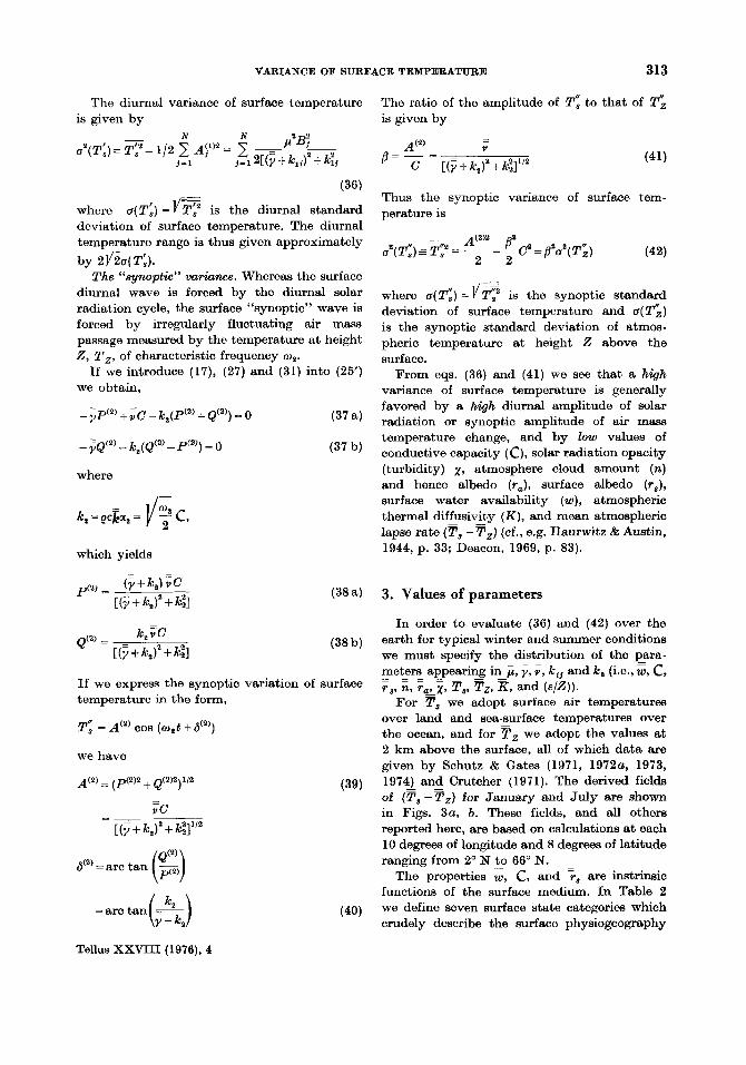
For T , we adopt surface air temperatures over land and sea-surface temperatures over the ocean, and for T , we adopt the values at 2 km above the surface, all of which data are given by Schutz & Gates (1971, 1972a, 1973, 1974) and Crutcher (1971). The derived fields of (F , -T,) for January and July are shown in Figs. 3a, b. These fields, and all others reported here, are based on calculations a t each 10 degrees of longitude and 8 degrees of latitude ranging from 2’ N to 66’ N.

The properties E, c, and r, are instrinsic functions of the surface medium. In Table 2 we define seven surface state categories which crudely describe the surface physiogeography

~ _ _ - ~- _ _ - ~ ~- - -



~- Fig. 3a. Field of (T,-T,) with 2 = 2 k m for January, in K.

Fig. 3b. Field of (T -Tz) with 2 = 2 km for July, in K.



Table 2. Surface physiogeographic categories, and typical values of surface parameters c =&, w, and is

-

C ~

Category Characteristics (loa J m-a K-' sec-li2) w T S

Land, 3-month rainfall (mm day- < 0.5

0.5-1.5 1.5-3.0 3.0-6.0

Ice or snow Summer tundra Ocean

6.0

-l) 12 14 16 18 20 16 16

1000

0.50 0.70 0.80 0.90 1.00 0.20 0.90 1.00

0.35 0.30 0.25 0.20 0.15 Table 1 Table 1 Table 1

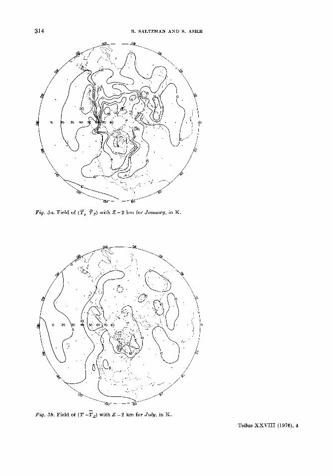
(cf., Saltzman 1967, Table 3). In Fig. 4a, b we show the northern hemisphere distribution of these categories for January and July, respectively, based on the precipitation data given by Schutz & Gates (1972a, b) .

The values of the water availability 6, and the conductive capacity c = (pit) , appropriate for the different surface states are shown in the first two columns of Table 2 (cf. Priestley, 1959). The surface albedo rs is also a function of surface state, but, in addition depends on the mean angle of incidence of the solar beam (particularly for ice and ocean) and hence is a function of latitude and season [note that we are neglecting the diurnal variation of rs due to the change in angle of incidence and phase change of snow (Dirmhirn & Eaton, 1975)l. The values adopted for the albedo of ice (or snow) and ocean, are given as a function of latitude in Table 1 , and are based mainly on data given by Budyko (1974). The albedo of land surface is mainly a function of type of soil and vegetation, which we shall here assume is related to rainfall. The values adopted are given in Table 2 (cf. Budyko, 1974, p. 54).

The albedo of the atmosphere is primarily a function of type and amount of cloudiness, and also of angle of incidence of solar radiation (a function of latitude and season). The parameterization adopted here is that proposed by Berliand (1960) (see Budyko, 1974, p. 45),

ra = [a(+) + b i ] n (44)

where n is the fractional cloud coverage, a(4 ) is given in Table 1, and b = 0.38. Here we use


the fields of n given by Schutz & Gates (1971, 1973, 1974) to compute both ra and the long wave radiation factor appearing in 7.

The mean clear-sky opacity of the atmosphere to solar radiation x is dependent on the path length of the solar radiation (assuming uniform turbidity) and hence is mainly a function of latitude and season. The values adopted here are listed in Table 1 (cf. Saltzman & Vernekar, 1971). In Figs. 5a , b we show the fields of p = [( 1 - Fs) (1 - r,) (1 - i)] for January and July, representing the fraction of the external radiation available for absorption at the surface.

The fundamental constants of the problem are

e cp = 1.00 x lo3 J kg-'K-' I? = 9.8 K km-1 u = 5.71 x lo-* W K-4 6 = 0.95 o1 = 2n/l day = 7.29 x oa = 2n/l week - 1.04 x 2 = 2 k m A = 2 7 3 K

= 1 kg m4 (air)

sec-l sec-'

The constants involved in the parameterization of the vertical flux of sensible heat by small scale eddy motions (Hk3') were chosen to yield a close fit to previous less detailed parameterizations of this flux (Saltzman, 1967, 1968; Saltzman & Vernekar, 1971). These values are

KO = 1.0 me sec-l yc = 5 K km-' E = 1 200 m3 sec-l K-I


Fig. 4a. Assigned values of physiogeographic type (see Table 1 ) for Janwlry.

Fig. 4 b . Assigned values of physiogeographic type (see Table 1 ) for July.



Fig. 5a. Field of p for January, in units of lo-'.

Fig. 5b . Field of p for July, in units of lo-'.



The above constants imply that

cg = c,c,6uA4 = 1.27 W m-2 K-’ c8 = 46aA3(c, - c z c 7 ) = 1.04 W m-z K-I cl0 = 36uA4(c, - c zc , ) = 213 W m-* c I 1 = czc,60A5 = 347 W m-* c , ~ = p p / Z = 0.5 J m-4 K-’ cI3 = p,(r - y c ) = 4.8 J m-4

The constants el through c7 were given in Section 2 .

4. Results

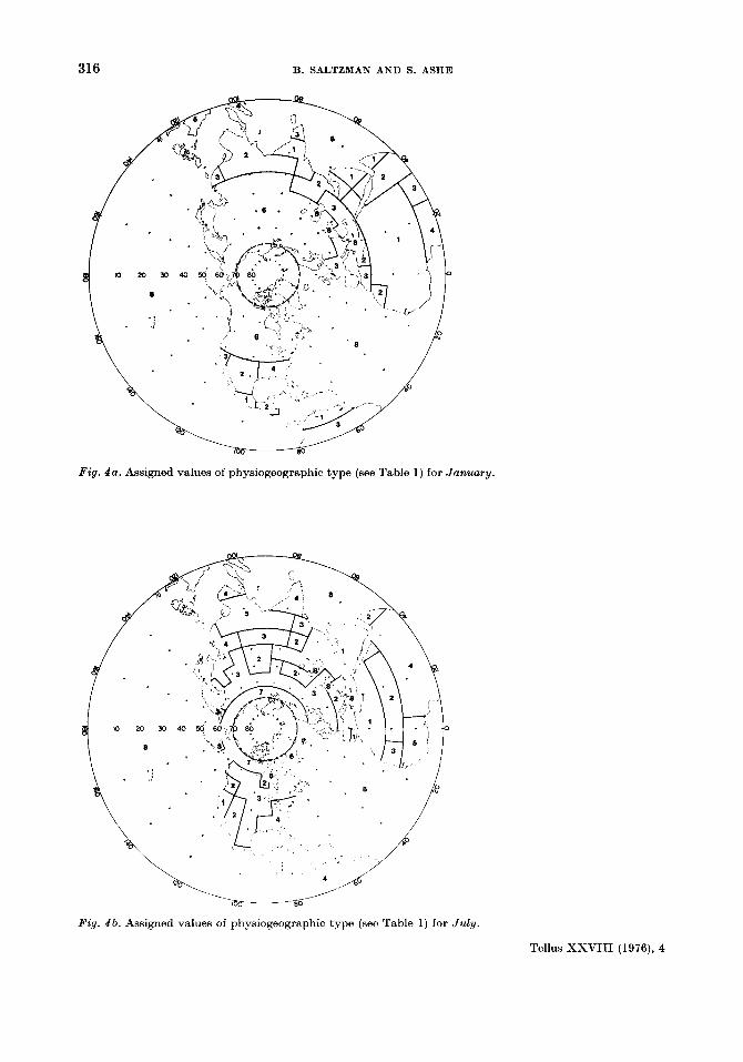
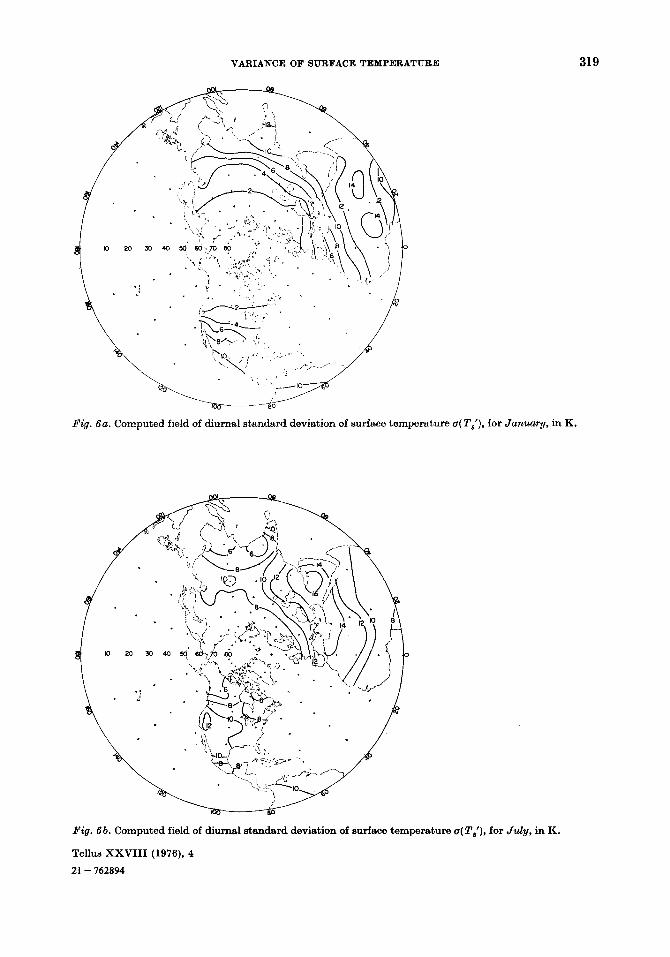
I’he diirrnal variance. Using the above values of parameters we can compute from (36) tho northern hemisphere distribution of the diurnal standard deviations of surface temperature a(T:). These are shown in Figs. 6 a arid 6b for January and July, respectively. As noted previously, to convert a ( ~ : ) to a measure of the diurnal temperature range we must multiply by roughly 21/2=2.8.

In Section 2 we remarked that the values of u( T:) obtained here apply to the surface “activc layer” that, in the limit, represents the air- surface “interface”. Hence these values should be somewliat larger than would be measured at air “shelter-level” (e.g. 1.5 m), perhaps by nearly a factor of two (cf. Fritz, 1963; Sasamori, 1970). Thus, to convert our a(T1) values to estimates of the near-surface air temperature ranges we should multiply them by 1/ 2 = 1.4.

The ocean responses are not shown on the maps bccanse they are more than an order of magnitude weaker than the continental responses. This is a consequence of the relatively large conductive capacity of the ocean. In Fig. 7 we show the zonal mean latitude distribution of u(T:) over ocean, this being very nearly the same as the oceanic latitudinal distribution at any given longitude. We note that these values are larger in summer than in winter, especially in high latitudes. Since we have taken the ocean values of c to be a constant ( lo5 J m-z K-l sec-4) for all latitudes and seasons, these distributions are mainly the consequence of the variations in the diurnal amplitude of incoming solar radiation. We can expect a somewhat wider departure between the slimmer and winter curves, particularly in high latitudes, when some allowance is made for the relatively higher values of c that prevail in the ocean in winter due to decreased thermal stratification

1-

and increased surface winds. However this modification should not alter the general magnitude of the computed ocean values of a(T:), which are in good agreement with observations (cf. Deacon 1969, Table 12).

Over the continents we find the highest values of a(T:) in regions where the diurnal amplitude of solar radiation reaching the surface is a maximum and where relatively arid conditions prevail. In general, the distribution is more zonal in winter than in summer, demonstrating the importance of the meridional gradient of the diurnal amplitude of solar radiation in winter (see Table 1 ) . The relatively weaker meridional gradient of a strong diurnal amplitude of solar radiation in July allows the influence of non-zonal physiogeographic features, such as those embodied in p, to be felt more strongly in this season.

Comparisons with observations of the diurnal surface temperature wave at selected continental stations, reported by Chang (1958), show reason- ably good agreement.

As is clear from the relative results for continent and oceans, the single most important surface influence on the global distribution of the diurnal temperature amplitude is the conductive capacity c. However, for the variations of u(T:) within continents the effects of water availability (w), and the albedo of the atmosphere ( ra) and surface ( rs ) are of equal or greater importance, and even more dominating than these surface and atmospheric parameters are the externally imposed gradients of the diurnal amplitude of radiation (particularly in winter).

Two influences on u(T1) that are not ade- quately taken into account in this treatment are those of topography and sea-breezes. Although, as noted above, we have used the obscrved values of (T,-T,) appropriate to the smoothed topography, we have at the same time neglected tho fact in mountain areas there should prevail lower values of the opacity x and water vapor pressnre e than would be appropriate for sea- level, both of which would lead to higher diurnal variances. On the other hand, at sea-level stations adjacent to the coasts we can expect somewhat lower diurnal variations than are representative of nearby inland points due to the ameliorating effects of sea-breeze circulations, particularly in summer.

The synoptic variance. I n Figs. 8a and 8 b we show the fields of ,!? (ratio of amplitudes



Fig. 6a. Computed field of diurnal standard deviation of surface temperature (I( !Ps'), for January, in K.

a( Ti), for in K.

320 B. SALTZMAN AND 9. ASHE

20 x) 40 50 60 70 90

I O ~ L l - . . L A 2

LATITUDE (ON)

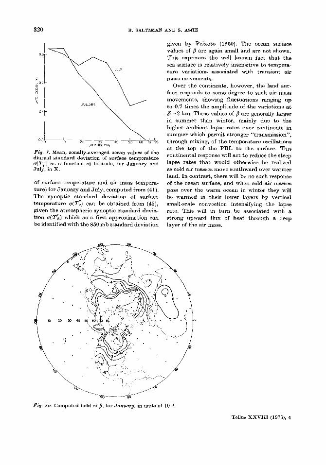
Pig. 7. Mean, zonally-averaged ocean values of the diurnal standard deviation of surface temperature u(T,’) as a function of latitude, for January and July, in K.

of surface temperature and air mass temperature) for January and July, computed from (41). The synoptic standard deviation of surface temperature a(!I$) can be obtained from (42), given the atmospheric synoptic standard deviation u ( T i ) which as a first approximation can be identified with the 850 mb standard deviation

given by Peixoto (1960). The ocean surface values of B are again small and are not shown. This expresses the well known fact that the sea surface is relatively insensitive to temperature variations associated with transient air mass movements.

Over the continents, however, the land surface responds to some degree to such air mass movements, showing fluctuations ranging up to 0.7 times the amplitude of the variations a t 2 = 2 km. These values of B are generally larger in summer than winter, mainly due to the higher ambient lapse rates over continents in summer which permit stronger “transmission”, through mixing, of the temperature oscillations a t the top of the PBL to the surface. This continental response will act to reduce the steep lapse rates that would otherwise be realized as cold air masses move southward over warmer land. In contrast, there will be no such response of the ocean surface, and when cold air masses pass over the warm ocean in winter they will be warmed in their lower layers by vertical small-scale convection intensifying the lapse rate. This will in turn be associated with a strong upward flux of heat through a deep layer of the air mass.

Fig. 8u. Computed field of B, for January, in units of 10-l.

Tollus XXVIII (197G), 4


Fig. 86. Computed field of B, for July, in units of 10-l.

Whereas the diurnal variation is a maximum a t the interface and is somewhat diminished at the shelter level, the synoptic variation would be larger a t the shelter level than a t the interface. Thus should be uniformly closer to unity a t the shelter level, even over the oceans.

5. Conclusions

In brief summary, we have shown that reasonable first estimates of the global field of diurnal and synoptic (i.e., cyclone-scale) variance of surface temperature can be obtained from a knowledge of the solar radiation distribution, the mean state of the free atmosphere, and the intrinsic physical properties of the earth’s surface. The formulas expressing this dependence can easily be incorporated into statistical- dynamical models of climate. Moreover, they can be applied to specific geographic locations or specific time periods by prescribing the

surface and ambient atmospheric conditions (e.g., cloud amount, lapse rate, water availability) appropriate for these locations or periods, which may depart from the average conditions specified here.

There is clearly room for improvement of the parameterizations and of the particular specifi- cation of parameters used here. In particular, it would seem of benefit to allow for time varia- bility of certain parameters held fixed at monthly mean values in this study (e.g., cloud amount, atmospheric diffusivity, surface albedo), to allow explicitly for all the effects of topographic height and sea breeze circulations along coasts, and to seek greater local fidelity and resolution of the physiogeographic field.

Acknowledgement

This research was supported by the Atmos- pheric Sciences Section of the National Science Foundation under grants ATM 75-00351 and ATM 75-21814.


B. SALTZMAN AND S. ASHE

REFERENCES

Budyko, M. I. 1974. Climate and life. Academic Press, New York, pp. 508.

Carslaw, H. S. & Jaeger, J. C. 1947. Conduction of heat in solids. Clarendon Press, Oxford.

Chang, J.-H. 1958. around temperature, vol. 1. Harvard Univ., Blue Hills Meteorological Observa- tory, pp. 300.

Crutcher, H. L. 1971. Selected meridional cross sections of heights, temperatures and dew points for the northern hemisphere. NAVAIR 50-1C-59 Naval Weather Service Command, Washington, D.C.

Deacon, E. L. 1969. Physical processes near the surface of the earth. World survery of climatology, vol. 2 (ed. H. Flohn). Elsevier Publ. Co., pp. 39-104.

Deardorff, J. W. 1972. Theoretical expression for the countergradient vertical heat flux. J . aeophys. Res. 77, 5900-5904.

Dirmhirn, I. & Eaton, F. D. 1975. Some characteristics of the albedo of snow. J . Appl. Meteorol. 14, 375-379.

Fritz, S. 1963. The diurnal variation of ground temperature as measured from TIROS 11. J . Appl. Meteorol. 2, 645-648.

Haurwitz, B. & Austin, J. M. 1944. Climatology. McGraw-Hill, New York, pp. 410.

Jaeger, J. C. & Johnson, C. H. 1953. Note on diurnal temperature variation. aeofis. Pura e Appl. 24, 10P106.

Jefferson, M. 1918. The real temperatures throughout North and South America. The Qeographical Rev. 6 , 240-267.

Lonnquist, 0. 1962. On the diurnal variation of surface temperature. Tellus 14, 96-101.

Peixoto, J. P. 1960. Hemispheric temperature conditions during the year 1950. Sci. Rpt. No. 4, M . I . T . Planetary Circulations Project, Contract No. A F 19(604)-6108, pp. 211.

Priestley, C. H. B. 1959. Turbulent transfer in the lower atmosphere. University of Chicago Press, pp. 130.

Saltzman, B. 1967. On the theory of the mean temperature of the earth’s surface. Tellus 19, 219-229.

Saltzman, B. 1968. Steady state solutions for axially-symmetric climatic variables. Pure and Appl. Geophysics 69, 237-259.

Saltzman, B. 1973. Parametrization of hemispheric heating and temperature variance fields in the lower troposphere. Pure and Appl. Qeophysics 105, 890-899.

Saltzman, B. & Ashe, S. 1976. Parametrization of the monthly mean vertical heat transfer a t the earth’s surface. Tellus. 28, 323 -332.

Saltzman, B. & Vernekar, A. D. 1971. An equi- librium solution for the axiallysymmetric com- ponent of the earth’s macroclimate. J . Qeophys. Res. 76, 1498-1524.

Sasamori, T. 1970. A numerical study of atmospheric and soil boundary layers. J . Atmos. Sci. 27, 1122-1137.

Schutz, C. & Gates, W. L. 1971. Qlobal climatic data for surface, 800 mb, 400 mb: January. The Rand Corp., Santa Monica, California. R-915- ARPA, pp. 173.

Schutz, C. & Gates, W. L. 1972a. Qlobat climatic data for surface, 800 mb, 400 mb: July. The Rand Corp., Santja Monica, California, R-1029-ARPA, pp. 180.

Schutz, C. & Gates, W. L. 1972b. Supplemental global climatic data: January. The Rand Corp., Santa Monica, California, R-915/1-ARPA, pp. 41.

Schutz, C. & Gates, W. L. 1973. Supplemental global climatic data: January. The Rand Corp., Santa Monica, California, R-915/2-ARPA, pp. 37.

Schutz, C. & Gates, W. L. 1974. Supplemental global climatic data: July. The Rand Corp., Santa Monica, California, R-1029/1-ARPA, pp. 38.

Smagorinsky, J. 1963. General circulation experi- ments with the primitive equations. Mo. Weath. Rev. 91, 99-164.


the variance of surface temperature due to diurnal and cyclone-scale forcing

Documents