the value of operational flexibility in the presence of...
TRANSCRIPT

The Value of Operational Flexibility in the Presenceof Input and Output Price Uncertainties with Oil
Refining Applications
Lingxiu Dong, Panos KouvelisOlin Business School, Washington University in St. Louis, St. Louis, MO 63130, USA
[email protected], [email protected]
Xiaole WuSchool of Management, Fudan University, Shanghai 200433, China
Refining is indispensable to almost every natural resource-based commodity industry. It involves a series of
complex processes that transform inputs with a wide range of quality characteristics into refined finished
products sold to end markets. In this paper, we take the perspective of a profit-maximizing refiner that
considers upgrading its existing simple refinery to include intermediate-conversion flexibility, i.e., the capa-
bility of converting heavy intermediate components to light ones. We present a stylized two-stage stochastic
programming model of a petroleum refinery to investigate the value drivers of conversion flexibility and the
impact of input and output market conditions on its economic potential. Conversion flexibility adds value
to refineries by either transforming a non-profitable situation into a profitable one (referred to as purchase
benefit) or improving profitability of an already profitable situation (referred to as unit revenue benefit). In
a real-data calibrated numerical study, we find the value of conversion flexibility (VoC) to be significant,
accounting for 40% of the expected profit with conversion, and the purchase benefit and unit revenue benefit
are equally important. Contrary to the intuition that, as a recourse action, conversion offers higher value for
greater input price volatility, we find that VoC may decrease in input price volatility due to the differential
impacts of increasing price volatility on the purchase benefit and the unit revenue benefit. Refineries also
vary in their range flexibility, i.e., the ability to accommodate a narrow or wide range of inputs of differ-
ent quality levels. Whether the range flexibility increases or decreases the value of conversion flexibility is
affected by the direction in which the refinery expands its processing range and the heaviness of crude oils.
History : Accepted by Martin Lariviere at Management Science in March, 2014.
1. Introduction
Many natural resource-based commodities share two common features. First, the quality of the
commodity varies by the geographic location where it is produced or harvested. Second, the eco-
nomic value of the commodity largely comes from the application of the derivative products that
originate from it, not from the direct use of the commodity itself. Refining is a key link in the
supply chain for these commodities; it is where raw materials from various origins and of different
1

2
qualities are transformed into refined derivative products of precise specifications, some of which
serve as feedstocks to downstream industries while others are consumed by the end users.
Take the petroleum refining industry, for example, which accounted for 2.55% of the world GDP
in 2004 (Dixon et al. 2007). The input, crude oil, is a mixture of molecules made of carbon and
hydrogen atoms. There are as many different crude oils as there are different oil fields and each field
yields its own particular quality. A rough form of characterization is the classification of “light” and
“heavy” crude oils. Compared with a heavy crude oil, a light crude oil contains a higher proportion
of the smaller hydrocarbon molecules with shorter carbon chains. Petroleum products obtained
from crude oil can be grouped into light (e.g., gasoline), medium (e.g., diesel), and heavy (e.g.,
lubricating oil) products based on the composition of the light and heavy distillates in the product.
Most petroleum products are not direct distillation outputs of crude oil. A refinery contains a
complex series of interconnected processing steps that separate crude oil into different fractions
according to their boiling ranges (in distillation units), alter the hydrocarbon molecular structure
and hence the quality of some of the lighter fractions (in reforming units), convert or crack heavy
fractions into lighter fractions (in conversion units), and finally blend intermediate fractions (in
blending units) to make acceptable products for sale to customers.
Refineries vary greatly in their abilities to convert heavy fractions to light fractions. Simple
refineries just separate the crude oil into their constituent petroleum products by distillation, while
complex refineries are able to convert heavy fractions to light fractions. Very complex refineries
have both the traditional type of conversion units and deep conversion units that can convert very
heavy fractions to light fractions. We refer to the capability of converting heavy fractions to light
fractions as intermediate-conversion flexibility (“conversion flexibility” hereafter). The rising price
of gasoline has been the main reason for refineries to upgrade existing simple refineries to complex
ones with conversion technologies, which give them the capability to derive more light fractions
and improve crude oil’s yield of light petroleum products. Operational flexibility in general is an
important asset to oil refineries. Although it is obvious that the value of conversion flexibility to a
refinery is influenced by conditions in crude oil and refined petroleum product markets, it is less
obvious how such value is affected by volatile price movement in these markets.
Conversion flexibility also interacts with other types of operational flexibility in the refinery.
An important flexibility of such is range flexibility : Refineries vary in the range of crude oils
they are capable of processing. As light and heavy crude oils have very different composition
and contaminant levels (e.g., sulfur, nitrogen, metals), a refinery that aims to accommodate a
range of crude oils requires a suite of processing technologies (e.g., hydrotreating, emission-control

3
technologies) to comply with federal and state environment protection regulations.1 As such, some
refineries are designed to efficiently process a particular type of crude oil or close substitutes, but
lack the flexibility to process other crude oils; others are able to process a wider range of heavy to
light crude oils. Because range flexibility enables a refinery to adjust its crude oil purchase portfolio
within its processing range, it offers an alternative means to affect the amount of heavy and light
fractions available for refining, which conversion flexibility achieves through thermal and chemical
processes. Is then conversion flexibility of less value to a refinery with wider crude oil processing
range? This is a natural question faced by refinery executives.
Existing studies on operational flexibility have primarily focused on flexibility on the input side
(e.g., the ability to process inputs of different qualities) or flexibility on the output side (e.g., the
ability to satisfy demand for one product with another). Conversion flexibility in oil refining, on the
other hand, operates on intermediates/works-in-process, and affects the refiner’s ability in blending
to respond to the output markets. The stage at which conversion takes place determines that
conversion flexibility plays a unique role linking the input procurement decision and the output
blending decision, and hence is different from those flexibilities studied in the existing literature.
In this paper we explore the value drivers of conversion flexibility and its interplay with range
flexibility. We address the following questions: First, how does conversion flexibility create value for
a refinery? How significant is this value? Second, how is the value of conversion flexibility influenced
by the price volatilities of crude oils and petroleum products? Finally, does a refinery with range
flexibility benefit more or less from having conversion flexibility than an otherwise identical refinery
that does not have range flexibility? In other words, are the two types of operational flexibility
strategic complements or substitutes? We study these questions within a short-term planning
horizon (weeks to several months) over which the main management objective is to maximize
the profit margin over variable costs.2 We make the following simplifying assumptions to obtain
a stylized two-stage stochastic programming model while capturing key features of oil refining
processes. First, we assume that any crude oil in the market is a mixture of two fractions, a light
fraction (DFl) and a heavy fraction (DFh), and crude oils differ in the relative proportions of the
two fractions. Second, as shown in Figure 1(a), the refining process we consider comprises three
distinct parts: (i) a distillation unit that separates the crude oil into DFl and DFh, (ii) a conversion
unit that converts the DFh to the DFl, and (iii) a blending unit that blends the two fractions to
1 In addition to crude oil processing equipment, there are also added requirements for crude oil pipelines.
2 When planning for a longer term (several years), the structure of the refinery and its operating costs are variablesthat must be decided in light of the company’s objectives.

4
lDF
qλ~
hDF
q
)~
1( λ−
q)~
( λλ −
lDF
qλ
hDF
q
)1( λ−
q
xL light end
product
xH heavy end
product
lDF
hDF
lDF
hDF
light end
product
heavy end
product
distillation unit conversion unit blending unit
conversion
(a) (b)
distillation unit conversion unit blending unit
Crude oilCrude oil
Figure 1 A stylized representation of a refinery process
make end petroleum products. In this stylized model, a refinery has conversion flexibility only if it
is equipped with a conversion unit; a refinery with range flexibility can process a range of heavy
to light crude oils, whereas a refinery without range flexibility processes a single crude oil.
We provide a preview of the main findings below. First, conversion flexibility adds value to the
refinery by increasing the unit revenue potential of crude oil via altering its composition of heavy
and light fractions. This benefit manifests itself in two forms: One is to enhance a refinery’s already
positive profit margin (unit revenue benefit), and the other is to change a negative margin to be
positive, enabling the refinery to afford the crude oil when the crude oil price is high (purchase
benefit). Both benefits contribute to the market value of the refinery. Our real-data calibrated
numerical study finds the two benefits are of similar magnitude, and together account for 20%-65%
of the profit with conversion for a wide range of refining capacities. Second, the crude oil and
petroleum product price volatilities have different impacts on the value of conversion flexibility:
The value of conversion flexibility first increases and then decreases as crude oil price variability
increases, but is not sensitive to petroleum product price variability. Finally, whether the range
flexibility increases or decreases the value of conversion flexibility is affected by the direction in
which the refinery expands its range flexibility and the heaviness of crude oils.
The organization of the paper is as follows. Section 2 reviews related literature. We present the
model for the single crude oil case in §3 and characterize the optimal policies in §4. The significance
of the value of conversion flexibility, and the impact of the crude oil and petroleum product market
conditions on it, are explored in §5. We extend the model to include range flexibility and study its
impact on the value of conversion flexibility in §6. We provide concluding remarks in §7.
2. Literature Review
Our work is related to several areas of literature, including coproduction systems, operational
flexibility, and applications of operations research in process industries. In this section, we review
the most relevant papers from each area and state our contribution to the literature.

5
Petroleum oil refining can be viewed as a coproduction system, where a single production run
yields multiple end products. Although coproduction systems vary greatly across industries (semi-
conductor, chemical, pulp and paper, agriculture, etc.), the existing literature focuses on features
that are common to a few industries, where the end products are vertically differentiated on quality
levels, and the yields for them are random; the manufacturer may use high-quality products to
satisfy demand for low-quality products (a form of output downward substitution). Main decisions
studied for such coproduction systems include the ex ante production quantity decision and the ex
post downward substitution and inventory allocation decisions. Papers that assume deterministic
demand include Bitran and Leong (1992) and Bitran and Gilbert (1994), whereas Hsu and Bassok
(1999) assume stochastic demand. Tomlin and Wang (2008) extend the literature by endogeniz-
ing the end product pricing decision and considering downconversion (converting high-speed chips
into low-speed chips) and allocation flexibilities. They examine the necessity of downconversion in
the presence/absence of optimal pricing. Kazaz (2008) considers the agricultural industry, where
harvest and yield are uncertain. The study takes the perspective of a farming firm that grows
and sells an agricultural commodity, and is focused on methods of battling supply uncertainties.
Motivated by the beef industry practice of meat packers sourcing inputs (fed cattle) using long-
term contracts and from spot markets, Boyabatli et al. (2011) study the optimal sourcing portfolio
and the impacts of upstream and downstream market conditions and processing characteristics on
the sourcing decision, with a focus on the value of using different procurement sources: long-term
contracts and spot markets.
In contrast to the above papers, we capture some unique features of oil refining not previously
studied in the coproduction literature. First, although output downward substitution is assumed
in the coproduction literature, many refined petroleum products have different applications, and
substitution among them is impossible; for example, a diesel-fueled car cannot use gasoline as
fuel. Conversion can be viewed as a form of substitution, however, at the intermediate level in
the form of converting low-value distillates into high-value distillates through chemical/thermal
reactions, which incurs non-negligible costs. Second, the input procurement decision in the oil
refining industry is more complex than the total production quantity decision common in the
coproduction literature (e.g., Bitran and Gilbert 1994). This is because inputs such as crude oils
differ in their quality and prices. Procurement managers not only need to decide the purchase
quantity, but also need to choose the best crude oil or a portfolio of crude oils. Third, unlike most
coproduction studies where random product yield is a key uncertainty considered, the distillation
yield of a crude oil characterized by the distillation curve is usually available to refineries before

6
the purchase of crude oil, and hence is not a random factor of concern.3 Uncertainties in crude
oil price and end product price, on the other hand, are main concerns, because refiners make
procurement and intermediate processing decisions in the face of output price uncertainty, and a
refiner’s profitability and the value of its operational flexibility are affected by the price movement
over time. Hence, input and output price uncertainty, as opposed to quantity uncertainty on the
output side, draws another distinction between this paper and the aforementioned coproduction
research.
The value of operational flexibility and its sensitivity to input/output market uncertainties are
among the main focuses of the operational flexibility literature. Many forms of operational flexibility
(e.g., component commonality, postponement, substitution, responsive pricing) can be viewed as
options/recourses that enable the firm to wisely utilize its resource after uncertainties are resolved.
Real options theory establishes that the value of options increases as the volatility of the underlying
uncertainty increases (Dixit and Pindyck 1994). The operational flexibility literature finds that
this conventional wisdom holds in some settings (e.g., flexible capacity in Chod and Rudi 2005)
but may fail to hold in others (e.g., postponing resource commitment in Chod et al. 2010a), the
latter due to the intricate interplay of operational factors and market uncertainty. Our paper shows
that in the context of oil refining, increasing input price volatility has differential impacts on the
value drivers of conversion flexibility, leading to case-dependent comparative statics of the value of
conversion flexibility.
A few papers in the operational flexibility literature consider the relationship among different
types of flexibility, for example, between downconversion and pricing flexibility as in Tomlin and
Wang (2008), between volume flexibility and product flexibility as in Goyal and Netessine (2011),
and among product mix flexibility, postponed resource commitment, and the ability to delay capac-
ity commitment as in Chod et al. (2012). We extend the literature by investigating the relationship
between two common types of flexibility, conversion flexibility and range flexibility in the oil refining
industry.
Process industries (including petroleum, coal, chemical) were among the first to adopt applied
operations research methodologies (e.g., Symonds 1955). The blending problem in the petrochemi-
cal industry has received extensive research attention (e.g., Martin and Lubin 1985, Candler 1991,
Ashayeri et al. 1994 and Karmarkar and Rajaram 2001). More complex planning and scheduling
3 The U.S. Bureau of Mines carries out distillation on thousands of crude oil samples from wells in all major producingfields. The results can be used without correction (Gary and Handwerk 1984). As discussed in Boyabatli (2011), thisis also the case in many agricultural industries.

7
decisions over multiple periods and for multiple connected production stages appear in Majozi and
Zhu (2001), Neumann et al. (2003), Maravelias and Grossman (2003), and Gaglioppa et al. (2008).
Most of these works assume a deterministic environment and resort to mathematical programming
for large-scale optimization or developing effective heuristic algorithms. The focus of our work is not
on offering an exact decision support tool but on offering insights that reveal the interconnection
of a number of sequential planning decisions under output price uncertainty, and on illustrating
the impact of the stochastic input and output environments on the value of conversion flexibility.
Recent works involving some integrated decision planning with applications in a process industry
are of a more stylized nature (e.g., Goel and Gutierrez 2006, Secomandi 2010, Wu and Chen 2010).
These papers, although characterizing optimal (sometimes multi-stage) operational policies in the
petroleum and natural gas industry, all consider production/inventory systems for a single product,
and therefore do not consider issues and challenges associated with coproduction and inputs in
various quality levels such as in our paper. Devalkar et al. (2011) consider optimal procurement,
processing, and trade decisions for a firm dealing with one input commodity and one or multiple
outputs, with a focus on investigating the benefit of the integrated decision-making rather than
the value of a particular process flexibility.
3. Model
We tailor our model to petroleum refining, where the inputs of the refinery are crude oils and the
outputs are petroleum products. We simplify crude oil’s multiple-fraction composition down to two
distillation fractions, a heavy distillation fraction DFh (made of large hydrocarbon molecules) and
a light distillation fraction DFl (made of small hydrocarbon molecules). For any given input, let λ
represent the proportion of DFl, and hence, the proportion of DFh is 1− λ. Petroleum products
can be derived by blending DFh and DFl in certain proportions. We assume there are two end
products traded in the petroleum spot market, a heavy end product (H) and a light end product
(L); blending a unit of light end product requires more of light fraction DFl than blending a
unit of heavy end product. The assumption of two end products is not restrictive but simplifies
the exposition and discussion significantly. The main insights of the two-product case hold in the
general case of N(> 2) end products (see Appendix E). For ease of exposition, hereafter we use
input and output in lieu of crude oil and end product, respectively.
We consider a refinery that purchases inputs from an input spot market and sells outputs to
an output spot market. The refinery can process input with DFl proportion λ ∈ [λh, λl], λh ≤ λl,
where input λh (λl) is the heaviest (lightest) input within its processing range. The refinery has
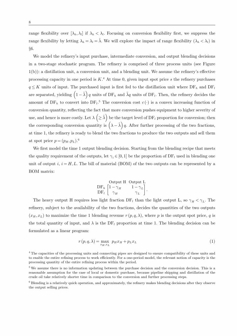
8
range flexibility over [λh, λl] if λh < λl. Focusing on conversion flexibility first, we suppress the
range flexibility by letting λh = λl = λ. We will explore the impact of range flexibility (λh <λl) in
§6.
We model the refinery’s input purchase, intermediate conversion, and output blending decisions
in a two-stage stochastic program. The refinery is comprised of three process units (see Figure
1(b)): a distillation unit, a conversion unit, and a blending unit. We assume the refinery’s effective
processing capacity in one period is K.4 At time 0, given input spot price s the refinery purchases
q ≤K units of input. The purchased input is first fed to the distillation unit where DFh and DFl
are separated, yielding(1− λ
)q units of DFh and λq units of DFl. Then, the refinery decides the
amount of DFh to convert into DFl.5 The conversion cost c (·) is a convex increasing function of
conversion quantity, reflecting the fact that more conversion pushes equipment to higher severity of
use, and hence is more costly. Let λ(≥ λ
)be the target level of DFl proportion for conversion; then
the corresponding conversion quantity is(λ− λ
)q. After further processing of the two fractions,
at time 1, the refinery is ready to blend the two fractions to produce the two outputs and sell them
at spot price p= (pH , pL).6
We first model the time 1 output blending decision. Starting from the blending recipe that meets
the quality requirement of the outputs, let γi ∈ [0,1] be the proportion of DFl used in blending one
unit of output i, i=H,L. The bill of material (BOM) of the two outputs can be represented by a
BOM matrix:
Output H Output L
DFh
DFl
[1− γH 1− γL
γH γL
].
The heavy output H requires less light fraction DFl than the light output L, so γH < γL. The
refinery, subject to the availability of the two fractions, decides the quantities of the two outputs
(xH , xL) to maximize the time 1 blending revenue r (p, q,λ), where p is the output spot price, q is
the total quantity of input, and λ is the DFl proportion at time 1. The blending decision can be
formulated as a linear program:
r (p, q,λ) = maxxH ,xL
pHxH + pLxL (1)
4 The capacities of the processing units and connecting pipes are designed to ensure compatibility of these units andto enable the entire refining process to work efficiently. For a one-period model, the relevant notion of capacity is theprocessing quantity of the entire refining process within the period.
5 We assume there is no information updating between the purchase decision and the conversion decision. This is areasonable assumption for the case of local or domestic purchase, because pipeline shipping and distillation of thecrude oil take relatively shorter time in comparison to the conversion and further processing steps.
6 Blending is a relatively quick operation, and approximately, the refinery makes blending decisions after they observethe output selling prices.

9
s.t. DFl : γHxH + γLxL ≤ λq (1a)
DFh : (1− γH)xH +(1− γL)xL ≤ (1−λ) q (1b)
xH , xL ≥ 0, (1c)
where (1a)-(1c) are the availability constraints of the two fractions and the non-negative production
constraint, respectively. We assume that unused distillation fractions have zero salvage value.
At time 0, the refinery purchases q units of crude oil with DFl proportion λ at a realized input
price s and then makes the fraction conversion decision to maximize the expected profit:
Π(λ, s
)= max
q∈[0,K],λ∈[λ,1]π(q, λ, λ
)− sq (2)
where π(q, λ, λ
)=Ep [r (p, q,λ)]− c
((λ− λ
)q). (2a)
The term sq in (2) represents the purchase cost of q units of input;7 π(q, λ, λ
)is the expected
revenue less conversion cost. In Expression (2a), bringing DFl proportion from the initial level λ
to the target level λ requires conversion of(λ− λ
)q units from DFh into DFl. The corresponding
conversion cost is c((
λ− λ)q); Ep [r (p, q,λ)] is the expected time 1 blending revenue, where Ep
represents taking expectation over time 1 output prices. Note that if the inter-temporal correlation
between s and p is positive, then the distribution of p is a function of s. For a refinery without
conversion flexibility, the constraint λ∈[λ,1
]in (2) is replaced by λ= λ.
We take the perspective of a refiner who considers upgrading an existing simple refinery to a
complex one with conversion units. Let Πc
(λ, s
)and Πo
(λ, s
)represent the profits of a refinery
at input price s with and without conversion flexibility, respectively, both at a given capacity level
K, the one-period processing capacity of the refinery without conversion flexibility.8 The difference
of these two profits, Πc
(λ, s
)−Πo
(λ, s
), represents the ex post value of conversion flexibility at
input spot price s. To calculate the short-term impact of conversion flexibility on the refinery’s
profitability, we define the value of conversion flexibility (VoC) for input λ as the expectation of this
profit difference, given by VoC(λ)=Es
[Πc
(λ, s
)−Πo
(λ, s
)], where Es represents taking expec-
tation over time 0 distribution of input price s. We will investigate the property of VoC analytically
under the assumption that input price s and output price p are uncorrelated, and then study the
7 To simplify exposition we normalize the unit processing cost (including power, chemicals, fuel costs, etc., excludingconversion cost) to 0, which does not have an impact on the qualitative insights.
8 It is not uncommon in practice that the refinery installs the new units to be compatible with the existing capacityof the refinery instead of adjusting the overall capacity of the plant to accommodate the new units, because capacityadjustment would require a radical overhaul of the refinery plant (equipment, pipes, control units) that could takeyears to complete, and would have to take into consideration (often inaccurate) demand and price trend forecastsover a long planning horizon (10− 20 years or more).
10
implications of the input-output price correlation numerically using a calibrated model, both in
§5. These studies shed light on the value drivers and economic potential of conversion flexibility in
various market environments. Before that, in §4, we characterize the optimal operational decisions,
for general price distributions and arbitrary inter-temporal input-output price correlation.
4. Optimal Operational Decisions
We first characterize the time 1 optimal blending decision, and then derive the time 0 optimal
conversion and purchase decisions.
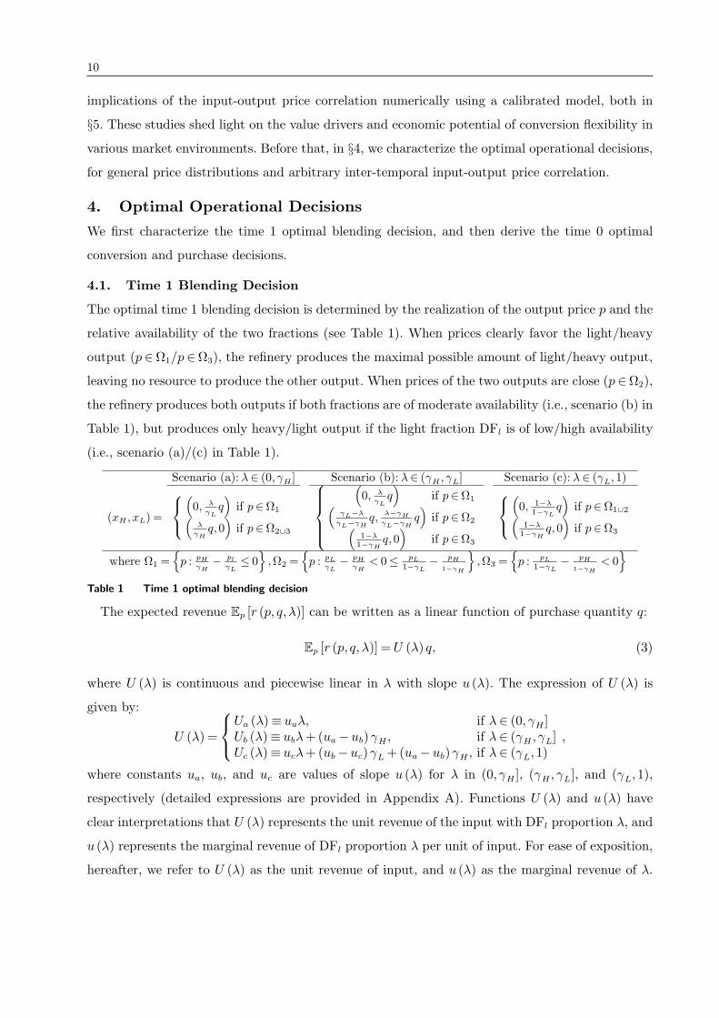
4.1. Time 1 Blending Decision
The optimal time 1 blending decision is determined by the realization of the output price p and the
relative availability of the two fractions (see Table 1). When prices clearly favor the light/heavy
output (p∈Ω1/p∈Ω3), the refinery produces the maximal possible amount of light/heavy output,
leaving no resource to produce the other output. When prices of the two outputs are close (p∈Ω2),
the refinery produces both outputs if both fractions are of moderate availability (i.e., scenario (b) in
Table 1), but produces only heavy/light output if the light fraction DFl is of low/high availability
(i.e., scenario (a)/(c) in Table 1).
Scenario (a): λ∈ (0, γH ] Scenario (b): λ∈ (γH , γL] Scenario (c): λ∈ (γL,1)
(xH , xL) =
(0, λ
γLq)
if p∈Ω1(λ
γHq,0
)if p∈Ω2∪3
(0, λ
γLq)
if p∈Ω1(γL−λ
γL−γHq, λ−γH
γL−γHq)if p∈Ω2(
1−λ1−γH
q,0)
if p∈Ω3
(0, 1−λ
1−γLq)
if p∈Ω1∪2(1−λ1−γH
q,0)if p∈Ω3
where Ω1 =p : pH
γH− pl
γL≤ 0
,Ω2 =
p : pL
γL− pH
γH< 0≤ pL
1−γL− pH
1−γH
,Ω3 =
p : pL
1−γL− pH
1−γH
< 0
Table 1 Time 1 optimal blending decision
The expected revenue Ep [r (p, q,λ)] can be written as a linear function of purchase quantity q:
Ep [r (p, q,λ)] =U (λ) q, (3)
where U (λ) is continuous and piecewise linear in λ with slope u (λ). The expression of U (λ) is
given by:
U (λ) =
Ua (λ)≡ uaλ, if λ∈ (0, γH ]Ub (λ)≡ ubλ+(ua −ub)γH , if λ∈ (γH , γL]Uc (λ)≡ ucλ+(ub −uc)γL +(ua −ub)γH , if λ∈ (γL,1)
,
where constants ua, ub, and uc are values of slope u (λ) for λ in (0, γH ], (γH , γL], and (γL,1),
respectively (detailed expressions are provided in Appendix A). Functions U (λ) and u (λ) have
clear interpretations that U (λ) represents the unit revenue of the input with DFl proportion λ, and
u (λ) represents the marginal revenue of DFl proportion λ per unit of input. For ease of exposition,
hereafter, we refer to U (λ) as the unit revenue of input, and u (λ) as the marginal revenue of λ.

11
Note that both U (λ) and u (λ) are functions of the distribution of time 1 output price p (which
in turn is a function of s if s and p are correlated); we suppress this dependence in notation for
expositional convenience. We will explore the impact of changes in the distribution of p in §5.
The marginal revenue of λ is positive when DFl is scarce, and negative when DFl is abundant.
That is, ua > 0 in scenario (a) and uc < 0 in scenario (c). When DFl is of moderate availability
(i.e., scenario (b)), the sign of the marginal revenue of λ, ub, depends on the distribution of output
price p. We will see in the next subsection that these values have direct implications for time 0
conversion decisions. Following convention, we let u+b = ub if ub > 0, and u+
b = 0 if ub ≤ 0. Also, the
terms increasing and decreasing are used in the weak sense.
4.2. Time 0 Purchase Quantity and Conversion Decisions
The time 0 purchase quantity and conversion decisions tie closely together, as shown by the fol-
lowing proposition.
Proposition 1. Given λ and s, the optimal purchase decision q∗ and the optimal conversion
decision λ∗ are summarized in the following tables
λ∈ (0, γH ]
u(λ)= ua
λ∈ (γH , γL]
u(λ)= ub
λ∈ (γL,1)
u(λ)= uc
c′ (0)∈ [ua,∞) (0) (0) (0)c′ (0)∈
[u+b , ua
)(1) (0) (0)
c′ (0)∈[0, u+
b
)(3) (2) (0)
where
Case q∗ λ∗
(0)
K, if s∈(0,U
(λ))
0, if s∈[U(λ),∞
) λ
(1)
K, if s∈(0,Ua
(λ))
max[0,min
[Qa
(λ, s
),K
]], if s∈
[Ua
(λ),∞
)(2)
K, if s∈(0,Ub
(λ))
max[0,min
[Qb
(λ, s
),K
]], if s∈
[Ub
(λ),∞
) Expression(4)
(3)
K, if s∈
(0,Ua
(λ))
min[Qa
(λ, s
),K
], if s∈
[Ua
(λ),Ub
(λ))
max[0,min
[Qb
(λ, s
),K
]]if s∈
[Ub
(λ),∞
)and in cases (1)-(3) λ∗ > λ is obtained from9
maxλ : λ∈
[λ,1
]and u (λ)− c′
((λ− λ
)q)≥ 0
, (4)
9 The detailed expression of λ∗ is provided in the proof of Proposition 1.

12
Qa
(λ, s
)is the solution to s=Ua (γH)−
(γH − λ
)c′((
γH − λ)Qa
), and Qb
(λ, s
)is the solution
to s=Ub (γL)−(γL − λ
)c′((
γL − λ)Qb
).
Cases (1)-(3) in Proposition 1 represent the cases where increasing the DFl proportion from the
initial level of λ to a higher level λ∗ via conversion is desirable. Conversion is used when a higher
DFl proportion enables the refinery to better respond to the output market in the blending stage,
i.e., when the marginal revenue of λ, u(λ)
is higher than the initial marginal conversion cost
c′ (0). Effectively, by changing the relative proportion of the heavy and light fractions, conversion
increases the unit revenue of the input from U(λ)
to U (λ∗). Conversion does not take place,
however, if the initial DFl proportion is already high or the initial marginal conversion cost is high,
i.e., Case (0) in Proposition 1.
Conversion plays a critical role in linking the output market and the input market. First, changes
in the output market condition directly affect the marginal revenue of λ, u (λ). For example,
when a shift in the output price distribution increases the value of marginal revenue ub from a
negative value to a positive one, the time 0 decision may change from no use of conversion to use
of conversion, i.e., from Case (0) to Case (2).10
Second, because the optimal target DFl proportion λ∗ balances the marginal revenue u (λ∗) and
the marginal conversion cost c′((
λ∗ − λ)q)
(see (4)), λ∗ is a function of both the initial DFl
proportion λ and the purchase quantity q. We can show that the optimal target level λ∗ decreases
convexly in quantity q (shown in the proof of Proposition 1). That is, the larger the quantity the
refinery purchases, the lower target DFl proportion λ∗ it can reach up from λ using conversion.
Thus, conversion flexibility affects the refinery’s input purchase quantity decision.
Figure 2 provides a graphical illustration of Proposition 1 in the(λ, s
)space, partitioning the
space into subregions based on the optimal purchase quantity and conversion decisions (q∗, λ∗).
When conversion is not desirable (Case (0) in Proposition 1, Figure 2(a)), the refinery’s optimal
purchase decision is a simple zero-or-full-capacity policy: If the spot price is lower than the unit
revenue of input, s < U(λ), then the refinery purchases up to full capacity K; otherwise, no
purchase. Represented in the(λ, s
)space, the feasible purchase region is bounded by the unit
revenue curve U(λ).
When conversion is desirable (Cases (1)-(3) in Proposition 1, Figures 2(b) and (c)), the benefit
of conversion flexibility manifests in two forms. When s < U(λ), the refinery purchases input
to full capacity K, and is able to extract a higher revenue than that without conversion (i.e.,
10 It is straightforward to show that if pH < pL (pH > pL) almost surely, then ub > 0 (ub < 0).

13
HK,ΛL
HK,ΛL
HK,ΛL
s
Λ
ΓH ΓL
HaL c'H0L Î @ua,¥L
H0,ΛL UHΛ
L
Gb
HK,ΛL Gc
HK,ΛL
Ga1HK,ΓH L
Ga3HQa,ΓH L
Ga2HK,Λ*L
s
Λ
Λ
aÖ
ΓHΓH ΓL
UaHΓH L-HΓH-ΛLc¢H0L
UaHΓH L-HΓH-ΛLc¢HHΓH-Λ
LKL
HbL c'H0L Î @ub,uaL
H0,ΛL
UbHΓLL-HΓL-ΛLc¢H0L
UaHΓH L-HΓH-ΛLc¢HHΓH-Λ
LKL UbHΓLL-HΓL-Λ
Lc¢HHΓL-Λ
LKL
Gb2
HK,Λ*LGc
HK,ΛL
Ga1
HK,ΓH L
Ga3
HQa,ΓH L
Ga2
HK,Λ*L
Gb3HQb,ΓLL
Gb1
HK,ΓLL
s
Λ
Λ
a
Ö
Λ
b
ÖΓH ΓLΛ
3
Ö1
H0,ΛL
HcL c'H0L Ε @0, ubL
Λ
a
Ö
: c¢HHΓH-Λ
a
Ö
LKL=ua
Λ
b
Ö
: c¢HHΓL-Λ
b
Ö
LKL=ub
Λ
3Ö
: c¢HHΓH-Λ
3Ö
LKL=ub
Gc=88Λ,s<: ΛÎ@ΓL,1D, s£UcHΛL<
Ga1=88Λ,s<: q*HΛ,sL=K, Λ*HK,ΛL=ΓH <
Ga2=88Λ,s<: q*HΛ,sL=K, c¢HHΛ*-ΛLKL=Max8ua,c¢H0L<<
Ga3=88Λ,s<: q*HΛ,sL=Qa, Λ*HQa,ΛL=ΓH <
Gb1=88Λ,s<: q*HΛ,sL=K, Λ*HK,ΛL=ΓL<
Gb2=88Λ,s<: q*HΛ,sL=K, c¢HHΛ*-ΛLKL=Max8ub,c¢H0L<<
Gb3=88Λ,s<: q*HΛ,sL=Qb, Λ*HQb,ΛL=ΓL<
Figure 2 Illustration of optimal purchase quantity and conversion decisions (q∗, λ∗) as functions of λ and s, for
ub > 0.
U (λ∗)K >U(λ)K). We refer to this form of benefit as the unit revenue benefit. When s≥U
(λ),
a refinery without conversion flexibility would not purchase the input, whereas a refinery with
conversion flexibility would purchase quantity Qa or Qb to balance the effective unit revenue of
input and the sum of the marginal conversion cost and the unit purchase cost, shown as the vertical
expansion of the purchase region in the(λ, s
)space. We refer to this form of benefit as the purchase
benefit of conversion flexibility.
We now characterize the unit revenue benefit and the purchase benefit of conversion flexibility
rigorously. Recall that the value of conversion flexibility is VoC(λ)= Es
[Πc
(λ, s
)−Πo
(λ, s
)],
and λ is the initial DFl proportion and λ∗ is the target DFl proportion for conversion. Let qc and qo
denote the optimal purchase quantities with and without conversion flexibility, respectively. Using
(2), (2a), and (3), the ex post value of conversion Πc
(λ, s
)−Πo
(λ, s
)at a realized input price s
can be written as:
Πc
(λ, s
)−Πo
(λ, s
)

14
=(U (λ∗)−U
(λ))
qo +(U (λ∗)− s) (qc − qo)− c((
λ∗ − λ)qc
)(5)
=
(U (λ∗)−U
(λ))
qo − c((
λ∗ − λ)qo
), if s <U
(λ), [unit revenue benefit]
(U (λ∗)− s) qc − c((
λ∗ − λ)qc
), if s≥U
(λ). [purchase benefit]
(6)
Observe from (5) that the ex post value of conversion comprises three terms. The first term(U (λ∗)−U
(λ))
qo represents the value increase directly from the increase of unit revenue; the
second term (U (λ∗)− s) (qc − qo) represents the value increase due to the increase of purchase
quantity; the third term c((
λ∗ − λ)qc
)is the conversion cost. The ex post value of conversion is the
value increases less the conversion cost. When the input price is low (i.e., s < U(λ)), qc = qo =K
and the refinery enjoys the unit revenue benefit only; when the input price is high (i.e., s≥U(λ)),
qo = 0 and the refinery enjoys the purchase benefit (see(6)). The VoC can be written as the sum of
the expected unit revenue benefit (URB) and the expected purchase benefit (PB):
V oC(λ)=Es<U(λ)
[Πc
(λ, s
)−Πo
(λ, s
)]︸ ︷︷ ︸
URB
+Es≥U(λ)
[Πc
(λ, s
)−Πo
(λ, s
)]︸ ︷︷ ︸
PB
.
5. Sensitivity Analysis
The purpose of this section is two-fold. First, we explore the significance of the value of conversion
flexibility and show that it is an important form of operational flexibility with great value potential.
We measure separately the expected unit revenue benefit (URB) and the expected purchase benefit
(PB) to understand which benefit is more important in a real-data calibrated parameter setting.
Second, we study the impact of capacity and the input and output market conditions (i.e., changes
in the variance of price distributions) on the value of conversion.
In each subsection, we first develop analytical results for the tractable case where time 0 input
price is uncorrelated with the time 1 output prices, and then resort to the numerical study to
investigate how the inter-temporal input-output price correlation might affect the results and
insights.
To calibrate the distribution of input and output prices, we obtain an empirical dataset consisting
of weekly crude oil and petroleum product prices between year 2000 and 2003 from the website of
the “Energy Information Administration (EIA),” the statistical and analytical agency within the
U.S. Department of Energy.11 We choose Saudi Arabia Arabian Light (AL) as the crude oil, and
gasoline and residual fuel oil as the light end product and the heavy end product, respectively.
To capture the inter-temporal input-output correlation we adopt a standard vector autoregressive
11 http://www.eia.doe.gov/, accessed April 2009.

15
(VAR) model, which implicitly assumes the prices follow normal distribution.12 Let χt = (s, pH , pL)T
t
represent time t price vector for crude oil, heavy, and light end products, where subscript t is the
time index measured in week, and superscript T is the transpose operator. We use the weekly price
data to calibrate the following VAR model:
(χt+1 −µ
)= η ·B · (χt −µ)+ e′, (7)
where µ= (µs, µH , µL)Tis the long-run average price vector, B is a 3× 3 coefficient matrix, and
e′ ∼N (0,Σ′). Parameter η is the inter-temporal input-output correlation factor. Before calibrating
the model parameters, we adjust all weekly prices for U.S. Consumer Price Index (CPI) inflation
and represent prices in constant year 2000 dollars, and then remove the monthly seasonality effect
from the deflated price data.13 µ is set to the overall mean of the adjusted data. We normalize the
real-world inter-temporal correlation factor η= 1, and then use the package “vars” for R language
to calibrate parameters B and Σ′. The R2 is approximately 90%. A typical lead time of two weeks
between time 0 (when purchase and conversion decisions are made) and time 1 (when blending
decision is made) is considered, and the 2-week VAR model for our study is derived below by
applying the calibrated 1-week VAR model iteratively twice:
(χt+2 −µ
)= η ·A · (χt −µ)+ e, (8)
where µ = (24.59,23.90,33.65), coefficient matrix A = B2, e = (es, eH , eL)T ∼ N (0,Σ), and Σ =
BΣ′BT +Σ′. Specifically,
A=
0.76 0.089 0.0050.063 0.87 −0.0180.45 0.31 0.43
, and Σ=
σ2es ρsHσesξσeH ρsLσesξσeL
ρsHσesξσeH (ξσeH)2
ρξ2σeHσeL
ρsLσesξσeL ρξ2σeHσeL (ξσeL)2
=
2.13 0.89 0.720.89 3.34 0.320.72 0.32 3.82
.
Most notation in Σ is self explanatory except ξ, which represents the common volatility factor
of the output prices (ξ is normalized to 1 in the calibration), reflecting the fact that the price
movement in the output market is often driven by a common set of economic factors.
To compute the value of conversion flexibility, VoC, we simulate time 0 prices using the stationary
distribution of (s, pH , pL)Tderived from the VAR model (8) by a standard approach (Cryer and
12 VAR model is commonly used to describe the evolution of crude oil, gasoline, and other commodity prices (see,e.g., Kilian 2009, Akram 2009, and Kilian 2010 for references).
13 Briefly, to remove the monthly seasonality effect, we let ςt denote deflated price vector at week t, ςt = χt + κm(t),where κm(t) is a deterministic vector that captures the monthly seasonality in spot prices with the subscript m (t)
indicating the month that week t falls in, and χt = (s, pH , pL)Tt is the deseasonalized price vector. We impose the
constraint that the 12 monthly seasonality vectors sum to zero vector, i.e.,∑m=12
m=1κm = 0.

16
Chan 2008), and then simulate time 1 prices according to (8).14 Let σs denote the standard deviation
of the stationary input price. In the ensuing subsections we will vary σs, ξ, and ρ to study the
impact of the variance of input price, variance of output prices, and correlation of output prices on
VoC, respectively. We vary the value of η around 1 in the numerical study to explore the impact
of the inter-temporal input-output price correlation on the sensitivity analysis results.15
Complying with the industry convention, we use the length of carbon chain as a quality index of
distillation fractions (heavy fractions typically have longer carbon chains).16 On the output side,
gasoline ranges from C4 to C12, and residual fuel oil ranges from C20 to C50 (Concawe 1998). DFl
(DFh) is defined as consisting of carbon chains ranging from C1 to C13 (C14 and up). Correspond-
ingly, Arabian Light yields 30% DFl after the distillation, so let λ= 0.3.17 Using the average carbon
chain length as the quality index, we derive γH = 0.2 and γL = 0.97 for the BOM matrix.18
We consider a refinery with the capacity of 3 mmtpa (million metric tons per annum), which is
equivalent to around 850,000 barrels every two weeks. Thus, we set K = 850 kbl (kbl stands for
thousand barrels). We model conversion cost using a quadratic function c (x) = τx+υx2, where x is
in kbl and c(x) is in k$. We let τ = 5.5, υ= 0.035, which corresponds to an average conversion cost of
4$ per barrel when the refinery is running at its full capacity (the calibration of the conversion cost
is discussed in the appendix). In the analytical study, we have normalized the unit distillation cost,
denoted as z, to be 0 for notational convenience. Setting z = 0 does not affect the qualitative results
of comparative statics, but will affect the magnitude of the profit and the value of conversion. A
positive z leads to a higher VoC relative to the expected profit. To reflect a realistic magnitude in
the numerical study, we set z = 1.3, which is 1/3 of the average conversion cost at the full capacity
(Favennec 2003).
5.1. Impact of Capacity (K)
A refinery’s processing capacity K influences the value potential of conversion flexibility as follows.
14 Unit root test shows our VAR model is stable. Stable VAR model implies for any t, the prices conform to stationarydistribution. Initializing time 0 prices at the stationary distribution allows us to assess the realistic magnitude ofvalue of conversion. The stationary distribution of (s, pH , pL)
T is given in Appendix D.
15 Changing η not only alters the inter-temporal correlation between input and output prices but also the variabilityof output prices. Therefore, the impact of increasing η is a combination of both effects.
16 Sulfur content is another common quality dimension in oil refining. However, most sulfur removal is accomplishedin a hydrotreater following the distillation process but before the conversion. Some residual sulfur remains in theblending stage. Heaviness is a more relevant quality dimension to conversion flexibility. Using one dimension of qualitymeasure allows analytical tractability.
17 http://www.theoildrum.com/story/2006/3/13/11938/9181
18 In our numerical study, we vary γH from 0.15 to 0.25, γL from 0.6 to 0.97, and find our qualitative sensitivityresults are robust against the choice of γH and γL.

17
Η increases from 0.8 to 1.2in step size of 0.2
500 1000 1500 2000
220
230
240
250
260
270
280
290
K
VoC
HaL
Η increases from 0.8 to 1.2in step size of 0.2
500 1000 1500 20000.0
0.1
0.2
0.3
0.4
0.5
0.6
0.7
K
VoC
Pc
HbL
Η increases from 0.8 to 1.2in step size of 0.2
500 1000 1500 2000
0.3
0.4
0.5
0.6
0.7
K
PB
VoC
HcL
Figure 3 Sensitivity of (a) VoC, (b) proportion of VoC in expected profit, and (c) proportion of purchase benefit
in VoC, to processing capacity K, for three levels of inter-temporal input-output price correlation
Proposition 2. Assume zero inter-temporal input-output price correlation and prices following
general distribution. There exists a threshold K, such that VoC increases concavely in K for K ∈(0, K
]and is constant in K for K ∈
(K,∞
), where for Cases (1) and (3) in Proposition 1 K
satisfies c′((
γH − λ)K)= ua and for Case (2) K satisfies c′
((γL − λ
)K)= ub.
Recall in the discussion of Proposition 1, the optimal conversion quantity(λ∗ − λ
)q should
never exceed a level that results in a marginal conversion cost being higher than the marginal
revenue of DFl proportion (see (4)). This means that the optimal conversion quantity has an upper
bound that is determined by the type of input it processes (i.e., the initial DFl proportion λ), the
conversion cost function c (·), and the marginal revenue of DFl proportion u (·). It implies that as the
capacity of the refinery increases, the value of conversion approaches and then remains at an upper
bound. Proposition 2 formalizes this intuition. Figure 3(a) shows that the result of Proposition 2
holds under the positive inter-temporal input-output price correlation (VoC is measured in k$, and
capacity in kbl). An implication of this result is that adding capacity alone cannot help increase
VoC when it reaches a plateau.
We first focus on the calibrated parameter setting with η normalized to 1, i.e., the thick curves
in all three figures. We find that VoC is significant, accounting for 20%− 65% of the profit with
conversion for the range of K corresponding to 8 mmtpa−1 mmtpa in Figure 3(b). At the base
capacity level (K = 3 mmtpa = 850 kbl), VoC accounts for approximately 40% of the profit with
conversion.
Recall that VoC is the sum of the expected unit revenue benefit (URB) and the expected purchase
benefit (PB). We investigate which of the two benefits plays a more significant role. Figure 3(c)

18
shows that PB accounts for approximately 60% of VoC and URB accounts for 40% of VoC. It
implies that both unit revenue benefit and purchase benefit are important. The significant purchase
benefit also explains the high VoC relative to the expected profit (Figure 3(b)), because when the
purchase benefit manifests, the profit equals the ex post value of conversion.
Figure 3 shows that as η increases, VoC increases but the proportion of VoC in expected profit
and the proportion of PB in VoC decrease. Intuitively, a stronger inter-temporal input-output price
correlation implies that a higher input price often results in a higher output price in the future;
therefore, the gross margin of a refinery increases as η increases, and so do the refinery’s profitability
and the value of conversion flexibility. The increase of the gross margin also implies the increase of
the unit revenue benefit of conversion flexibility, which explains the decreasing proportion of PB
in VoC and the decreasing proportion of VoC in expected profit.
5.2. Impact of Input Price Volatility on VoC
In this and the next subsections we explore how the value of conversion flexibility is influenced by
input and output market conditions such as changes in the variance and correlation of prices.
Because conversion is a recourse action taking place after the realization of the input spot price,
one might expect that VoC increases as the input price variability σs increases. Proposition 3 shows
that the impact of input price variability is influenced by the level of the mean input price, and
VoC can decrease in σs.
Proposition 3. Assume zero inter-temporal input-output price correlation and prices following
normal distribution. There exist two thresholds T1 and T2, T1 <T2, such that VoC decreases in σs
if µs ≤ T1, and VoC increases in σs if µs ≥ T2.
We can show that the unit revenue benefit is constant in the input price for s <U(λ), and the
purchase benefit decreases convexly in the input price for s ≥ U(λ)(Lemma 1, Appendix). For
this reason, we refer to the input price domain where the unit revenue benefit is in play as the
high-benefit region, and where the purchase benefit is in play as the low-benefit region of conversion
flexibility.
When the mean input price is low, the price realizations fall mainly in the low-price region, where
the refinery enjoys the unit revenue benefit, i.e., the high-benefit region. As the price variance
increases, more price realizations take place in the high-price region, where the refinery enjoys the
purchase benefit, i.e., the low-benefit region; thus, the value of conversion decreases.
When the mean input price is high, the price realizations fall mainly in the high-price region,
i.e., the low-benefit region. As the price variance increases, more price realizations take place in
the low-price region, i.e., the high-benefit region. Hence, the value of conversion increases.
19
Η = 1.2
Η = 1
Η = 0.8
2.0 2.5 3.0 3.5 4.0
220
230
240
250
260
270
280
Σs
VoC
HaL
Η = 1.2
Η = 1
Η = 0.8
2.0 2.5 3.0 3.5 4.0
80
100
120
140
160
Σs
URB
HbL
Η = 1.2
Η = 1
Η = 0.8
2.0 2.5 3.0 3.5 4.0
110
120
130
140
150
160
170
Σs
PB
HcL
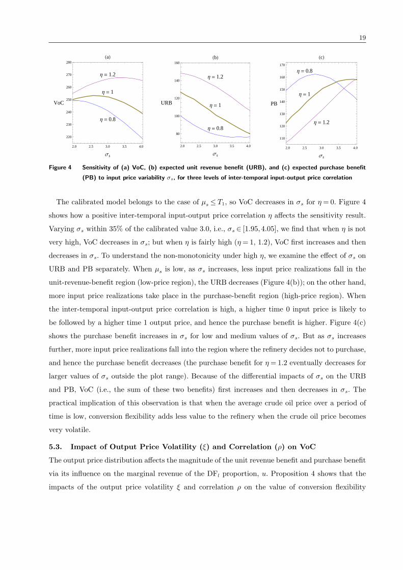
Figure 4 Sensitivity of (a) VoC, (b) expected unit revenue benefit (URB), and (c) expected purchase benefit
(PB) to input price variability σs, for three levels of inter-temporal input-output price correlation
The calibrated model belongs to the case of µs ≤ T1, so VoC decreases in σs for η = 0. Figure 4
shows how a positive inter-temporal input-output price correlation η affects the sensitivity result.
Varying σs within 35% of the calibrated value 3.0, i.e., σs ∈ [1.95,4.05], we find that when η is not
very high, VoC decreases in σs; but when η is fairly high (η= 1, 1.2), VoC first increases and then
decreases in σs. To understand the non-monotonicity under high η, we examine the effect of σs on
URB and PB separately. When µs is low, as σs increases, less input price realizations fall in the
unit-revenue-benefit region (low-price region), the URB decreases (Figure 4(b)); on the other hand,
more input price realizations take place in the purchase-benefit region (high-price region). When
the inter-temporal input-output price correlation is high, a higher time 0 input price is likely to
be followed by a higher time 1 output price, and hence the purchase benefit is higher. Figure 4(c)
shows the purchase benefit increases in σs for low and medium values of σs. But as σs increases
further, more input price realizations fall into the region where the refinery decides not to purchase,
and hence the purchase benefit decreases (the purchase benefit for η= 1.2 eventually decreases for
larger values of σs outside the plot range). Because of the differential impacts of σs on the URB
and PB, VoC (i.e., the sum of these two benefits) first increases and then decreases in σs. The
practical implication of this observation is that when the average crude oil price over a period of
time is low, conversion flexibility adds less value to the refinery when the crude oil price becomes
very volatile.
5.3. Impact of Output Price Volatility (ξ) and Correlation (ρ) on VoC
The output price distribution affects the magnitude of the unit revenue benefit and purchase benefit
via its influence on the marginal revenue of the DFl proportion, u. Proposition 4 shows that the
impacts of the output price volatility ξ and correlation ρ on the value of conversion flexibility

20
depend on the heaviness of the input (i.e., the initial DFl proportion λ) and the marginal conversion
cost.
Proposition 4. Assume zero inter-temporal input-output price correlation and prices following
normal distribution. (1) For Case (1) in Proposition 1, i.e., for c′ (0) ∈[u+b , ua
)and λ ∈ (0, γH ],
V oC increases in ξ and decreases in ρ. (2) For Cases (2) and (3) in Proposition 1, i.e., for
c′ (0) ∈[0, u+
b
)and λ ∈ (0, γL], there exist thresholds t1 and t2, such that V oC increases in ξ
if f pLγL
− pHγH
(0)/f pH1−γH
− pL1−γL
(0) ≤ t1, and V oC decreases in ρ if f pLγL
− pHγH
(0)/f pH1−γH
− pL1−γL
(0) ≤ t2,
where f pLγL
− pHγH
and f pH1−γH
− pL1−γL
are the probability density functions of pLγL
− pHγH
and pH1−γH
− pL1−γL
,
respectively.
When the input is heavy and conversion cost is moderate (Proposition 4(1)), conversion can
bring the DFl proportion to at most γH . This implies that in the blending stage, the refinery uses
up its scarce DFl and produces only one output, either heavy or light (Scenario (a) in Table 1). In
this situation, an increase of the maximum of the two output prices increases the marginal revenue
of DFl proportion. Increasing output price volatility or decreasing price correlation increases the
probability of high realizations of the maximum of the two output prices, and hence increases the
marginal revenue of DFl proportion and the value of conversion.
When the input is not very light and the conversion cost is low (Proposition 4(2)), conversion is
able to significantly increase the DFl proportion, but the refinery ends up with surplus DFl if the
realization of output prices favors the heavy output. If the current output price distribution favors
the heavy output (conditions f pLγL
− pHγH
(0)/f pH1−γH
− pL1−γL
(0)≤ t1 and f pLγL
− pHγH
(0)/f pH1−γH
− pL1−γL
(0)≤
t2 in Proposition 4(2)), then the marginal revenue of DFl proportion is low. Increasing price volatil-
ity or decreasing price correlation increases the likelihood that output prices favor the light output,
resulting in increasing the marginal revenue of DFl proportion and increasing the value of con-
version. In other words, increasing output price volatility or decreasing output price correlation is
likely to increase the value of conversion when the refinery processes a heavy input, or the current
output price distribution often leaves the refinery with surplus DFl. The conditions in Proposition
4(2) are sufficient conditions. If they fail, increasing price volatility or decreasing price correlation
may decrease the marginal revenue of DFl proportion. In the calibrated model, the output price
distribution is such that the refinery in most cases uses up both distillation fractions to blend both
heavy and light outputs, and remains so when variability or correlation of output prices changes.
Therefore, VoC is not sensitive to ξ or ρ.
21
6. Refinery with Range Flexibility
A refinery with range flexibility needs to determine a purchase portfolio of inputs within its pro-
cessing range. We formulate the input portfolio decision and characterize the optimal decision in
§6.1, and examine the impact of range flexibility on the value of conversion flexibility in §6.2.
6.1. Time 0 Input Portfolio Decision
Suppose that n crude oils traded in the input spot market fall into the refinery’s processing range
[λh, λl], λh < λl. Each input is represented by its DFl proportion λi and spot price si, i= 1, ..., n.
Let M represent this set of inputs, M = (λi, si) : i= 1, ..., n, with λh ≤ λ1 < ... < λn ≤ λl. Let I
be the index set of inputs that the refinery chooses to purchase and θ= (θj)j∈Ibe the proportion
vector of the chosen inputs in the portfolio, θj > 0,∑
j∈I θj = 1. Because the total available DFl
from distilling the portfolio of inputs is the sum of the DFl from each of the purchased inputs,
equivalently, one can view the portfolio of inputs as mixing the inputs into a “new” input according
to θ. The new input has a DFl proportion (spot price) equal to the linear combination of the DFl
proportions (spot prices) of the inputs in the portfolio. The input portfolio decision is given by
maxI⊆1,...,n,θ∈(0,1]|I|,Σj∈Iθj=1
Π(λ, s
)(9)
where λ=∑
j∈I θjλj, s=∑
j∈I θjsj, and Π(λ, s
)is defined in (2)-(2a). λ and s are the proportion
of DFl and the effective price of the new input, respectively.
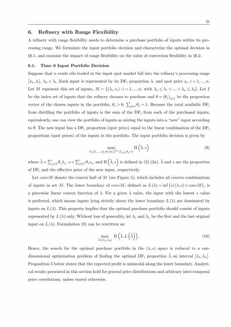
Let convM denote the convex hull of M (see Figure 5), which includes all convex combinations
of inputs in set M. The lower boundary of convM , defined as L (λ) = inf s| (λ, s)∈ convM, is
a piecewise linear convex function of λ. For a given λ value, the input with the lowest s value
is preferred, which means inputs lying strictly above the lower boundary L (λ) are dominated by
inputs on L (λ). This property implies that the optimal purchase portfolio should consist of inputs
represented by L (λ) only. Without loss of generality, let λ1 and λn be the first and the last original
input on L (λ). Formulation (9) can be rewritten as:
maxλ∈[λ1,λn]
Π(λ,L
(λ))
. (10)
Hence, the search for the optimal purchase portfolio in the (λ, s) space is reduced to a one-
dimensional optimization problem of finding the optimal DFl proportion λ on interval [λ1, λn] .
Proposition 5 below states that the expected profit is unimodal along the lower boundary. Analyti-
cal results presented in this section hold for general price distributions and arbitrary inter-temporal
price correlations, unless stated otherwise.

22
Hγ
Lγ
( )λuslope =
( )λ'Lslope =
4λ3
λ2
λ1
λ
s
λ
convM
original
Min inputs
( )λL
optimal theinput
Figure 5 Input selection in the absence of conversion flexibility when there are five original inputs in the market,
which are represented by round dots in the (λ, s) space
Proposition 5. Π(λ,L (λ)) is unimodal in λ.
Without loss of generality, we start the search of the optimal DFl proportion λ from λ1 and move
to higher λ values along L (λ). We first consider the simple case that the refinery does not have
conversion flexibility or conversion is not desirable (e.g., c′(0)>ua). In this case, determining the
optimal DFl proportion, λ, boils down to balancing the marginal cost of increasing λ, L′ (λ), and
the marginal revenue of λ, u (λ). Since L′ (λ) is piecewise constant and increases at λi (illustrated
in Figure 5) and u (λ) is piecewise constant and decreases at γH and γL, the optimal λ is the point
at which L′ (λ) exceeds u (λ) for the first time.
When the refinery has conversion flexibility and conversion is affordable (e.g., c′ (0) < u+b and
λ < γL), the input portfolio decision involves interesting tradeoffs. Starting from λ1 and moving
to higher λ values, the search of the optimal DFl proportion λ may stop earlier than when the
refinery does not have conversion flexibility. This happens when the marginal cost of increasing
λ, L′ (λ), exceeds the marginal conversion cost c′ ((λ∗ −λ) q∗), where λ∗ and q∗ are the optimal
target conversion level and optimal purchase quantity for input λ, respectively, because at that
point conversion is more cost effective than including more lighter inputs to increase the DFl
proportion. Thus, with conversion flexibility, the optimal λ is the point at which L′ (λ) exceeds
u (λ) or c′ ((λ∗ −λ) q∗), whichever happens first. The possibility that the search can stop earlier at
a heavier input implies that a refinery with conversion flexibility can make better use of heavier
crude oils in its processing range than a refinery without such flexibility.
The unimodal property of Π(λ,L (λ)) greatly simplifies the input search along L (λ), λ∈ [λ1, λn]:
As the search moves along L (λ) from low λ value to high λ value, once a local optimal input is
found, it is also the global optimal one.
6.2. Impact of Range Flexibility on Value of Conversion Flexibility
Refinery facilities vary by the range of crude oils they are designed to process. A refinery with a
processing range [λh, λl] is considered as having heavier- (lighter-) range flexibility than a refinery

23
that processes input λl (λh) only. Does conversion flexibility offer more value to a refinery with range
flexibility than to a single-input refinery? If yes, a refiner should choose among its refineries the one
with range flexibility to invest in conversion flexibility; otherwise, choose the refinery without range
flexibility to invest in conversion flexibility. To investigate how the value of conversion flexibility is
affected by range flexibility, we compare VoC of a refinery that processes input λl or λh only with
VoC of a refinery that has a processing range [λh, λl]. We define the latter as
VoC(λh, λl) =Es
[max
λ∈[λh,λl]Πc
(λ,L
(λ))
− maxλ∈[λh,λl]
Πo
(λ,L
(λ))]
,
where maxλ∈[λh,λl]Πc
(λ,L
(λ))
and maxλ∈[λh,λl]Πo
(λ,L
(λ))
, following the derivation for (10),
are the profits with and without conversion flexibility, respectively, and Es denotes taking expec-
tation over the time 0 spot prices s of inputs λh and λl.
Recall that VoC(λ) represents the value of conversion flexibility for single input λ. Proposition
6 compares VoC(λh, λl) and VoC(λl), and VoC(λh, λl) and VoC(λh).
Proposition 6. (1) The heavier-range flexibility enhances the value of conversion flexibility,
i.e., VoC(λh, λl) ≥VoC(λl). (2) Assume zero inter-temporal input-output price correlation. The
lighter-range flexibility enhances the value of conversion flexibility, i.e., VoC(λh, λl)≥VoC(λh), if
λl <λ†a, where λ†
a is the solution to c′((γH −λ†
a
)K)= ua.
The heavier-range flexibility allows the refinery to choose a heavier input over the light input
λl when the heavier input offers higher profit. When this happens, the unit revenue benefit or the
purchase benefit of conversion is greater for the heavier input than for the light input. This implies
Proposition 6(1).
One might conclude that the lighter-range flexibility diminishes the value of conversion by con-
jecturing less conversion is needed by lighter inputs. This intuition, however, does not hold when
both inputs are very heavy (λh < λl < λ†a), as shown in Proposition 6(2). To understand the rea-
son, let us consider four representative input price scenarios and compare the ex post value of
conversion for the light and heavy inputs. Scenario (i): Spot prices for both inputs are low such
that both inputs fall into unit-revenue-benefit region. In this case, because both inputs are quite
heavy, they require the same amount of conversion if being processed and thus have the same ex
post value of conversion. Scenario (ii): Spot prices for both inputs are high such that both inputs
fall into purchase-benefit region. In this case, the profit of each input is derived completely from
the purchase benefit of conversion. If the lighter input has a higher profit, then it also has a higher
ex post value of conversion. Scenario (iii): The lighter input falls into unit-revenue-benefit region
24
(i.e., high-benefit region), but the heavy input falls into purchase-benefit region (i.e., low-benefit
region). Again, the lighter input has higher ex post value of conversion. In these three scenarios,
the lighter input enjoys higher or at least the same level of ex post value of conversion. Scenario
(iv): The lighter input falls into purchase-benefit region (i.e., low-benefit region), but the heavy
input falls into unit-revenue-benefit region (i.e., high-benefit region). In this case, the heavy input
is chosen over the lighter input, and thus lighter-range flexibility does not affect the ex post value
of conversion. The above four scenarios together imply that lighter-range flexibility enhances the
value of conversion.
When the lighter input is indeed light (λl > λ†a), in above Scenario (i), this much lighter input
needs less conversion and has lower ex post value of conversion than the heavy one. Therefore, it
is inconclusive whether the lighter-range flexibility enhances or diminishes the value of conversion.
In other words, the intuition that heavier-range flexibility enhances the value of conversion
flexibility holds. The intuition that lighter-range flexibility diminishes the value of conversion does
not hold when the lighter input is also very heavy, in which case the lighter-range flexibility enhances
the value of conversion; it may hold, however, only when the lighter input is light enough. This
insight on the interplay of range flexibility and conversion flexibility holds even with the presence
of inter-temporal input-output price correlation; however, in this case it is hard to characterize the
threshold for input heaviness, λ†a, because the marginal revenue of DFl proportion u (·) depends
on the time 0 input price realization.
To understand the magnitude of the impact of lighter- and heavier-range flexibility on VoC,
we conducted two sets of numerical study. In the first study, we choose West Texas Intermediate
(WTI) as the lighter input; in the second study, we choose Nigeria Bonny Light (NBL) as the
lighter input. Arabian Light (AL) is used as the heavier input in both studies. The DFl proportion
for WTI is λWTI = 0.43, for NBL is λNBL = 0.37, and recall for AL λAL = 0.3.19 Note that WTI is
lighter than NBL.
In each study, we use the following VAR model.
(χt+2 −µ
)= η ·A · (χt −µ)+ e, (11)
where χ = (sH , sL, pH , pL)Twith sH and sL representing the spot price of the heavier input and
lighter input, respectively, µ= (µsH , µsL, µH , µL)Tis the long-run average price vector of χ, A is a
4× 4 coefficient matrix, and e= (esH , esL, eH , eL)T ∼N (0,Σ). The calibrated parameters for each
study are summarized in Appendix D.
19 http://www.theoildrum.com/story/2006/3/13/11938/9181

25
The impact of heavier-range flexibility, defined as (VoC(λh, λl)−VoC(λl))/VoC(λl) , and the
impact of lighter-range flexibility, defined as (VoC(λh, λl)−VoC(λh))/VoC(λh) for both studies are
summarized in Table 2.
[λh, λl] ηImpact of heavier-range flexibility (%)
Impact of lighter-range flexibility (%)
0.8 +499 −3.92[λAL, λWTI ] 1 +337 −3.93
1.2 +166 −4.130.8 +80.4 +1.16
[λAL, λNBL] 1 +61.4 +0.581.2 +42.4 +0.11
Table 2 Impacts of the heavier- and lighter-range flexibility on the value of conversion flexibility
Table 2 shows that heavier-range flexibility can enhance the value of conversion flexibility signif-
icantly. For a refinery currently processing a very light input, say WTI, expanding the capability
to process the heavier input AL can enhance VoC by 337% for the calibrated parameter setting
(η= 1). For a refinery currently processing a light input NBL, which is not as light as WTI, the
impact of heavier-range flexibility on VoC, although lower, remains significant, enhancing VoC by
61.4%.
Compared to the impact of heavier-range flexibility, the impact of lighter-range flexibility on
VoC is modest. For a refinery currently processing heavy input AL, expanding to process the very
light input WTI decreases the value of conversion by 3.93% for the calibrated parameter setting,
whereas, expanding its processing range to include lighter input NBL, which is heavier than WTI,
can increase the value of conversion by 0.58% for the calibrated parameter setting. These numerical
results echo the above discussion: Lighter-range flexibility does not necessarily diminish the value
of conversion flexibility; it can enhance its value when the lighter input is not very light.
7. Conclusions
Commodity industries such as petroleum oil refining face tremendous price uncertainties in both
input and output markets. Refiners’ survival and profitability in volatile marketplaces depend on
their ability to maximally utilize the process flexibility of their refining facilities, and to make
prudent procurement decisions. This paper includes a number of important, basic decisions of
an oil refinery (input purchase, intermediate processing, and output blending) in a stylized two-
stage stochastic programming model to study the economic potential of a process flexibility for
intermediate processing, namely, conversion flexibility, and the impacts of market conditions on
the value of this flexibility.

26
Conversion flexibility in the oil refining process, converting heavy fraction to light fraction after
distillation, serves to bridge the gap between the diversity of inputs available in the input market
and the specific requirement of the outputs from the output market. The benefits of conversion
flexibility are manifested in two forms: One is to enhance the unit revenue of the procured input
(unit revenue benefit), and the other is to enable the refinery to afford the input when the input price
is high (purchase benefit). Our real-data calibrated numerical study shows that VoC is significant,
accounting for approximately 40% of the profit with conversion. The unit revenue benefit and
the purchase benefit are of similar importance, with the former contributing 40% and the latter
contributing 60% of the value of conversion.
The unit revenue benefit and the purchase benefit are realized in different ranges of input price.
Increasing input price variance can affect expected values of the two benefits in the same direction or
different directions. For example, our real-data calibrated numerical study shows that the purchase
benefit increases for a small increase of input price variance, but decreases together with the unit
revenue benefit as the input price variance increases further. Hence, VoC first increases and then
decreases as the input price variance increases. The impact of output price volatility on VoC,
on the other hand, is affected by the heaviness of the input that the refinery processes and the
conversion cost. The real-data based numerical study shows that VoC is not sensitive to output
market conditions. These insights are helpful to refinery executives when it is pertinent to assess
the value of conversion flexibility over a long time horizon consisting of many short high-volatility
and low-volatility periods.
Conversion flexibility interacts with range flexibility of the refinery in an interesting way. Expand-
ing a refinery’s input processing range towards heavier inputs can enhance VoC significantly.
Surprisingly, expanding the processing range towards lighter inputs does not necessarily diminish
VoC, although it does when the lighter input is indeed quite light. The lighter-range flexibility can
enhance VoC when the new input, although relatively lighter than the current input, is still not
very light. Also interestingly, VoC increases with the processing capacity of a refinery only up to a
capacity threshold, beyond which VoC remains constant. These findings are useful when refinery
executives contemplate whether and how the decision on conversion flexibility investment should
be jointly considered with capacity or/and range flexibility.
We conclude the paper with a brief discussion of extensions of the model and future research.
First, most of the analytical results established in this paper can be extended to the case of more
than two outputs and the case of light-to-heavy conversion (see details in Appendix E). Second,
although the refinery considered in this paper is a price taker in the input and output markets, a
27
realistic assumption for many petroleum refineries, some large refiners can influence prices in both
markets through their purchases and sales. It is worthwhile to investigate the use of conversion
flexibility in the presence of pricing power as well as the interplay of conversion and pricing. Third,
our model focuses on the input spot purchase and the output spot sale. When the decision-maker
is risk neutral and the trading market and the capital market are frictionless, spot trading and
long-term contracts are separable decisions; otherwise, long-term contracts and spot trading should
be considered jointly (e.g., Dong and Liu 2007, Boyabatli et al. 2011). In the latter case, whether
the employment of operational flexibility reduces or increases the need for financial hedging of
commodity price risk, although beyond the scope of this paper, is an important question for future
research (see Chod et al. 2010b).
Finally, conversion is also an important form of operational flexibility in agricultural oil refining.
Oil extracted from oil seeds (e.g., soybeans, sunflower, canola, and safflower seeds) is hydrogenated
to generate intermediates called basestocks. A wide range of basestocks can be produced with the
hydrogenation process, depending on the conditions used and the degree of saturation and/or iso-
merization (O’Brien 2010). Basestocks are then blended according to recipes to produce different
types of end products (e.g., edible oil, shortenings, margarines). Hydrogenation plays a similar role
in agricultural oil refining as conversion does in petroleum oil refining. Although great similarity
exists between the oil refining processes of the two industries, the agricultural industry has lim-
ited, often illiquid spot markets for the end products, and the refineries face different challenges.
Investigating the roles of operational flexibility in dealing with these challenges can be a fruitful
direction for future research.
Acknowledgments
The authors thank the Associate Editor and the three anonymous referees for their many constructive
comments, which have helped to improve the quality of the paper significantly. The authors also thank
Atique Malik, PHD for insightful discussions on petroleum refining processes. The third author is supported
by the National Natural Science Foundation of China [Grant 71201036].
References
Akram, Q. F. 2009. Commodity prices, interest rates and the dollar. Energy Econom. 31(6) 838–851.
Ashayeri, J., A. G. M. van Eijs, P. Nederstigt. 1994. Blending modeling in process manufacturing: A case
study. Eur. J. Oper. Res. 72(3) 460–468.
Bitran, G. R., S. M. Gilbert. 1994. Co-production processes with random yields in the semiconductor
industry. Oper. Res. 42(3) 476–491.

28
Bitran, G. R., T. Y. Leong. 1992. Deterministic approximations to co-production problems with service
constraints and random yields. Management Sci. 38(5) 724–742.
Boyabatli, O. 2011. Supply management in multi-product firms with fixed proportions technology. Working
paper. Singapore Management University, Singapore.
Boyabatli, O., P. R. Kleindorfer, S. R. Koontz. 2011. Integrating long-term and short-term contracting in
beef supply chains. Management Sci. 57(10) 1771–1787.
Candler, W. 1991. Coal blending with acceptance sampling. Computers & Oper. Res. 16(6) 591–596.
Chod, J., D. Pyke, N. Rudi. 2010a. The value of flexibility in make-to-order systems: the effect of demand
correlation. Oper. Res. 58(4) 834–848.
Chod, J., N. Rudi. 2005. Resource flexibility with responsive pricing. Oper. Res. 53(3) 532–548.
Chod, J., N. Rudi, J. A. Van Mieghem. 2010b. Operational flexibility and financial hedging: complements
or substitutes. Management Sci. 56(6) 1030–1045.
Chod, J., N. Rudi, J. A. Van Mieghem. 2012. Mix, time, and volume flexibility: valuation and corporate
diversification. Rev. Bus. Econom. Lit. 57(3).
Concawe. 1998. Heavy fuel oils. Tech. rep., CONCAWE, Brussels.
Cryer, J. D., K. Chan. 2008. Time Series Analysis: With Applications in R. Springer.
Devalkar, S. K., R. Anupindi, A. Sinha. 2011. Integrated optimization of procurement, processing, and trade
of commodities. Oper. Res. 59(6) 1369–1381.
Dixit, A. K., R. S. Pindyck. 1994. Investment Under Uncertainty . Princeton University Press, New Jersey.
Dixon, P. B., S. Osborne, M. T. Rimmer. 2007. The economy-wide effects in the United States of replacing
crude petroleum with biomass. Working paper.
Dong, L., H. Liu. 2007. Equilibrium forward contracts on nonstorable commodities in the presence of market
power. Oper. Res. 55(1) 128–145.
Favennec, J. 2003. Petroleum Refining V.5: Refinery Operations and Management . Editions Technip.
Gaglioppa, F., L. A. Miller, S. Benjaafar. 2008. Multitask and multistage production planning and scheduling
for process industries. Oper. Res. 56(4) 1010–1025.
Gary, J. H., G. E. Handwerk. 1984. Petroleum refining technology and economics. 2nd ed. Marcel Dekker,
Inc., New York, New York.
Goel, A., G. Gutierrez. 2006. Integrating commodity markets in the optimal procurement policies of a
stochastic inventory system. Working paper. University of Texas, Austin.
Goyal, M., S. Netessine. 2011. Volume flexibility, product flexibility, or both: The role of demand correlation
and product substitution. Manufacturing Service Oper. Management 13(2) 180–193.
Hsu, A., Y. Bassok. 1999. Random yield and random demand in a production system with downward
substitution. Oper. Res. 47(2) 277–290.
29
Karmarkar, U. S., K. Rajaram. 2001. Grade selection and blending to optimize quality and cost. Oper. Res.
49(2) 1–10.
Kazaz, B. 2008. Pricing and production planning under supply uncertainty. Working paper. Syracuse
University.
Kilian, L. 2009. Not all oil price shocks are alike: Disentangling demand and supply shocks in the crude oil
market. American Econom. Rev. 99(3) 1053–1069.
Kilian, L. 2010. Explaining fluctuations in gasoline prices: A joint model of the global crude oil market and
the u.s. retail gasoline market. Energy J. 31(2) 87–104.
Majozi, T., X. X. Zhu. 2001. A novel continuous-time milp formulation for multipurpose batch plants. 1.
short-term scheduling. Ind. Eng. Chem. Res. 40(25) 5935–5949.
Maravelias, C. T., I. Grossman. 2003. Minimization of the makespan with a discrete-time state-task network
formulation. Ind. Eng. Chem. Res. 42 6252–6257.
Martin, C. H., S. Lubin. 1985. Optimization modeling for business planning at trumbull asphalt. Interfaces
15 66–72.
Neumann, K., C. Schwindt, N. Trautmann. 2003. Advanced production scheduling for batch plants in process
industries. H. O. Gunther, P. van Beek, eds., Advanced Planning and Scheduling Solutions in Process
Industry . Springer-Verlag, Berlin, 43–71.
O’Brien, R. D. 2010. Soybean oil modification. L. A. Johnson, P. J. White, R. Galloway, eds., Soybeans -
Chemistry, Production Processing, and Utilization, vol. 2, chap. 13. AOCS Publishing.
Secomandi, N. 2010. Optimal commodity trading with a capacitated storage asset. Management Sci. 56
449–467.
Symonds, G. H. 1955. Linear programming: The solution of refinery problems. Esso Standard Oil Company,
New York.
Tomlin, B., Y. Wang. 2008. Pricing and operational recourse in coproduction systems. Management Sci.
54(3) 522–537.
Wu, Q. O., H. Chen. 2010. Optimal control and equilibrium behavior of production-inventory systems.
Management Sci. 56(8) 1362–1379.
Appendix A: Expression of u (λ)
u (λ) =
ua ≡EΩ1
[pLγL
]+EΩ2∪3
[pHγH
](> 0) , if λ∈ (0, γH ]
ub ≡EΩ1
[pLγL
]+EΩ2
[−pH+pLγL−γH
]+EΩ3
[−pH1−γH
], if λ∈ (γH , γL]
uc ≡−EΩ1∪2
[pL
1−γL
]−EΩ3
[pH
1−γH
](< 0) , if λ∈ (γL,1)
, (12)
where EΩi[·] =
∫ ∫Ωi
·f (pH , pL)dpHdpL, and f (pH , pL) is the joint probability density function of pH and pL.
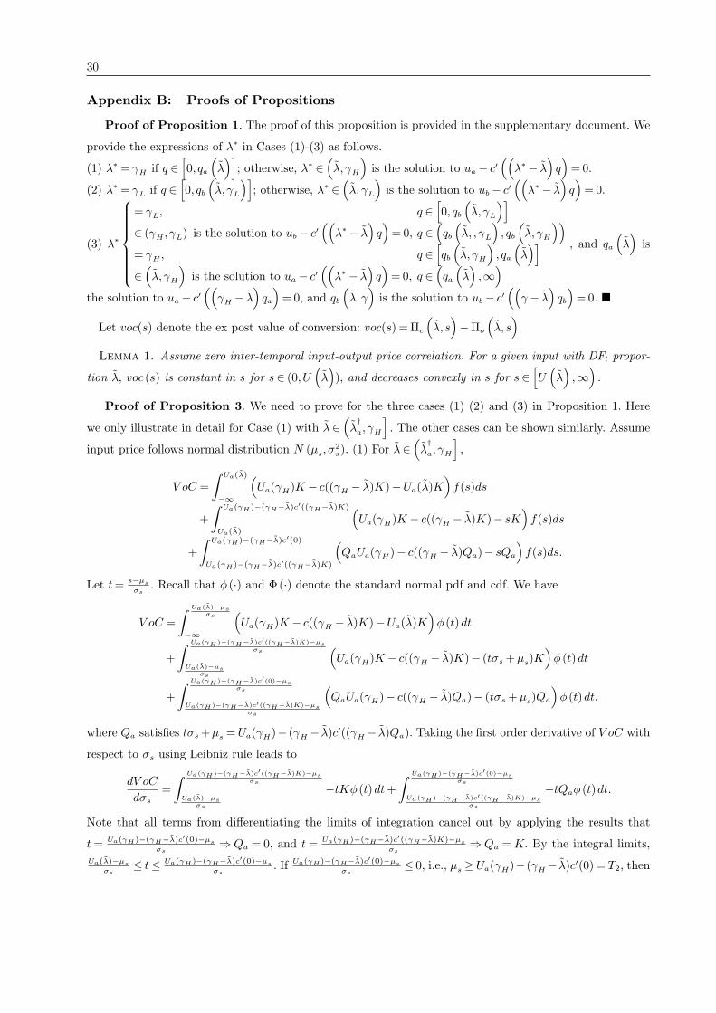
30
Appendix B: Proofs of Propositions
Proof of Proposition 1. The proof of this proposition is provided in the supplementary document. We
provide the expressions of λ∗ in Cases (1)-(3) as follows.
(1) λ∗ = γH if q ∈[0, qa
(λ)]
; otherwise, λ∗ ∈(λ, γH
)is the solution to ua − c′
((λ∗ − λ
)q)= 0.
(2) λ∗ = γL if q ∈[0, qb
(λ, γL
)]; otherwise, λ∗ ∈
(λ, γL
)is the solution to ub − c′
((λ∗ − λ
)q)= 0.
(3) λ∗
= γL, q ∈[0, qb
(λ, γL
)]∈ (γH , γL) is the solution to ub − c′
((λ∗ − λ
)q)= 0, q ∈
(qb
(λ, , γL
), qb
(λ, γH
))= γH , q ∈
[qb
(λ, γH
), qa
(λ)]
∈(λ, γH
)is the solution to ua − c′
((λ∗ − λ
)q)= 0, q ∈
(qa
(λ),∞
) , and qa
(λ)
is
the solution to ua − c′((
γH − λ)qa
)= 0, and qb
(λ, γ
)is the solution to ub − c′
((γ− λ
)qb
)= 0.
Let voc(s) denote the ex post value of conversion: voc(s) =Πc
(λ, s
)−Πo
(λ, s
).
Lemma 1. Assume zero inter-temporal input-output price correlation. For a given input with DFl propor-
tion λ, voc (s) is constant in s for s∈ (0,U(λ)), and decreases convexly in s for s∈
[U(λ),∞
).
Proof of Proposition 3. We need to prove for the three cases (1) (2) and (3) in Proposition 1. Here
we only illustrate in detail for Case (1) with λ∈(λ†a, γH
]. The other cases can be shown similarly. Assume
input price follows normal distribution N (µs, σ2s). (1) For λ∈
(λ†a, γH
],
V oC =
∫ Ua(λ)
−∞
(Ua(γH)K − c((γH − λ)K)−Ua(λ)K
)f(s)ds
+
∫ Ua(γH)−(γH−λ)c′((γH−λ)K)
Ua(λ)
(Ua(γH)K − c((γH − λ)K)− sK
)f(s)ds
+
∫ Ua(γH)−(γH−λ)c′(0)
Ua(γH)−(γH−λ)c′((γH−λ)K)
(QaUa(γH)− c((γH − λ)Qa)− sQa
)f(s)ds.
Let t= s−µs
σs. Recall that ϕ (·) and Φ(·) denote the standard normal pdf and cdf. We have
V oC =
∫ Ua(λ)−µsσs
−∞
(Ua(γH)K − c((γH − λ)K)−Ua(λ)K
)ϕ (t)dt
+
∫ Ua(γH )−(γH−λ)c′((γH−λ)K)−µsσs
Ua(λ)−µsσs
(Ua(γH)K − c((γH − λ)K)− (tσs +µs)K
)ϕ (t)dt
+
∫ Ua(γH )−(γH−λ)c′(0)−µsσs
Ua(γH )−(γH−λ)c′((γH−λ)K)−µsσs
(QaUa(γH)− c((γH − λ)Qa)− (tσs +µs)Qa
)ϕ (t)dt,
where Qa satisfies tσs+µs =Ua(γH)− (γH − λ)c′((γH − λ)Qa). Taking the first order derivative of V oC with
respect to σs using Leibniz rule leads to
dV oC
dσs
=
∫ Ua(γH )−(γH−λ)c′((γH−λ)K)−µsσs
Ua(λ)−µsσs
−tKϕ (t)dt+
∫ Ua(γH )−(γH−λ)c′(0)−µsσs
Ua(γH )−(γH−λ)c′((γH−λ)K)−µsσs
−tQaϕ (t)dt.
Note that all terms from differentiating the limits of integration cancel out by applying the results that
t= Ua(γH)−(γH−λ)c′(0)−µs
σs⇒Qa = 0, and t= Ua(γH)−(γH−λ)c′((γH−λ)K)−µs
σs⇒Qa =K. By the integral limits,
Ua(λ)−µs
σs≤ t≤ Ua(γH)−(γH−λ)c′(0)−µs
σs. If Ua(γH)−(γH−λ)c′(0)−µs
σs≤ 0, i.e., µs ≥Ua(γH)−(γH − λ)c′(0) = T2, then

31
t ≤ 0, which implies dV oCdσs
> 0. If Ua(λ)−µs
σs≥ 0, i.e., µs ≤ Ua(λ) = T1, then t ≥ 0, which implies dV oC
dσs< 0.
Similarly, we can show for Case (1) with λ∈(0, λ
†a
], T2 =Ua(γH)− (γH − λ)c′(0) and T1 =Ua(λ) as well; for
Case (2), T1 =Ub(λ) and T2 =Ub(γL)−(γL− λ)c′(0); for Case (3), T1 =Ua(λ) and T2 =Ub(γL)−(γL− λ)c′(0).
The following lemma facilitates the proof of Proposition 4.
Lemma 2. Assume zero inter-temporal input-output price correlation and prices following normal distri-
bution. (a) U (λ) increases in ξ and decreases in ρ. (b) ua increases in ξ and decreases in ρ. (c) There exist
thresholds t1 and t2, such that ub increases in ξ if and only if (iff) f pLγL
− pHγH
(0)/f pH1−γH
− pL1−γL
(0)≤ t1, and ub
decreases in ρ iff f pLγL
− pHγH
(0)/f pH1−γH
− pL1−γL
(0)≤ t2.
Proof of Proposition 4. λ is the input’s DFl proportion. f(·) denotes the pdf of input price s. V oC =
Es[voc (s)]. If s≥U(λ), Πo(λ, s) = 0 and thus voc (s) =Πc(λ, s), which increases in ξ but decreases in ρ by
Lemma 2 (a). If s < U(λ), then voc (s) =Πc(λ, s)−Πo(λ, s) and q∗ =K always. Let λ∗ be the target level
of DFl proportion after conversion (λ∗ ≤ γL). Let e denote ξ or ρ. There are three cases of dvoc(s)
dedepending
on the relationship between γH , λ, and λ∗.
dvoc (s)
de=
K
(λ∗ − λ
)dua
de, λ≤ λ∗ ≤ γH ,
K(λ∗ − λ
)dub
de, γH ≤ λ≤ λ∗,
K (λ∗ − γH)dub
de+K
(γH − λ
)dua
de, λ≤ γH ≤ λ∗.
(B.1)
Combining the two intervals of s, we have dV oCde
=∫ U(λ)s¯
dvoc(s)
def (s)ds+
∫ s
U(λ)dvoc(s)
def (s)ds (The terms from
differentiating the limits of integration cancel out). As discussed above, in the second term dvoc(s)
dξ> 0 and
dvoc(s)
dρ< 0. dvoc(s)
dein the first term can involve dua
de, or dub
de, or both dub
deand dua
de. If λ≤ λ∗ ≤ γH , then
dvoc(s)
de
in the first term only involves dua
de. By Lemma 2 (b), dua
dξ> 0 and dua
dρ< 0. Thus, we also have dvoc(s)
dξ> 0
and dvoc(s)
dρ< 0 in the first term. This leads to dV oC
dξ> 0 and dV oC
dρ< 0. Since c′ (0) ∈ [ub, ua) and λ ∈ (0, γH ]
imply λ ≤ λ∗ ≤ γH , (1) is proved. If λ∗ > γH ,dvoc(s)
dein the first term involves ub. Let X = pL
γL− pH
γHand
Y = pH1−γH
− pL1−γL
. The sign of dub
dedepends on the magnitude of fX(0)
fY (0)by Lemma 2 (c). When fX(0)
fY (0)≤ t1,
dub
dξ≥ 0. Then dvoc(s)
dξ≥ 0 in the first term. Together with dvoc(s)
dξ> 0 in the second term, dV oC
dξ> 0. When
fX(0)
fY (0)> t1,
dub
dξ< 0. Then dvoc(s)
dξ< 0 must (may) hold in the first term for γH ≤ λ≤ λ∗
(λ≤ γH ≤ λ∗
). Since
dvoc(s)
dξ> 0 in the second term, dV oC
dξcan be either positive or negative depending on the weight the input
price distribution puts over the two integral domains in the two terms. When fX(0)
fY (0)≤ t2,
dub
dρ≤ 0. Then
dvoc(s)
dρ≤ 0 in the first term. Together with dvoc(s)
dρ< 0 in the second term, dV oC
dρ< 0. When fX(0)
fY (0)> t2,
dub
dρ> 0.
Then dvoc(s)
dρ> 0 must (may) hold in the first term for γH ≤ λ≤ λ∗
(λ≤ γH ≤ λ∗
). Since dvoc(s)
dρ< 0 in the
second term, dV oCdρ
can be either positive or negative depending on the weight the input price distribution
puts over the two integral domains in the two terms. c′ (0) ∈ [0, ub) and λ ∈ (0, γL] imply that conversion
takes place, and either λ∗ >γH or λ∗ ≤ γH . For both cases, the conditions in (2) are sufficient.Proof of Proposition 6. (1) First we consider the impact of heavier-range flexibility on the value of
conversion. Without heavier-range flexibility, the refinery can only purchase input λl; with heavier-range
32
flexibility, the refinery can purchase any mix of inputs λh and λl. We consider two cases: In the first
case, heavier-range flexibility does not affect the purchase decision if without conversion flexibility, i.e.,
maxλ∈[λh,λl]Πo (λ,L (λ)) =Πo (λl,L (λl)). Since maxλ∈[λh,λl]Πc (λ,L (λ))≥Πc (λl,L (λl)), vocr ≥ voco, where
vocr (voco) denotes the ex post value of conversion with (without) range flexibility. In the second case,
maxλ∈[λh,λl]Πo (λ,L (λ))> Πo (λl,L (λl)). For the second case, we use matrix to represent all possible pur-
chase decisions under the four flexibility scenarios. Each entry corresponds to one scenario as shown below:[with both conversion and range flexibility, with only range flexibilitywith only conversion flexibility, with neither flexibility
].
All possible purchase decisions in the second case are summarized in the following six matrices, where λ∗
is the optimal crude oil to purchase with both flexibilities, and 0 stands for no purchasing.
(1) (2) (3) (4) (5) (6)[λ∗ λh
0 0
] [λ∗ γi
0 0
] [λ∗ λh
λl 0
] [λ∗ γH
λl 0
] [λ∗ λh
λl λl
] [λ γH
λl λl
]When it is optimal not to purchase without range flexibility, as Matrices (1) and (2) show, voco =
0, which implies vocr ≥ voco. For Matrix (3): No purchasing if with neither conversion nor range flex-
ibility implies sl > U (λl) . Purchasing input λl if with conversion but no range flexibility implies that
sl is in Ga3 (or Gb3) , or in Ga1 (or Gb1) but above U (λl). All these cases can be shown to lead to
vocr ≥ voco, but we only illustrate the case of sl in Ga3 as follows: voco = Πc (λl, sl) = Ua (γH)Qa −c ((γH −λl)Qa)− slQa; vocr = Πc (λ
∗, s∗)−Πo (λh, sh) ≥ Πc (λh, sh)−Πo (λh, sh); Assume sh is in Ga1(the
case of sh in Ga2 can be shown similarly), then vocr − voco ≥ Πc (λh, sh) − Πo (λh, sh) − Πc (λl, sl) =
ua (γH −λh)K − c ((γH −λh)K) − (γH −λl)Qac′((γH −λl)Qa) − c ((γH −λl)Qa) > ua (γH −λh)K −
c′((γH −λh)K) ((γH −λh)K − (γH −λl)Qa)−(γH −λl)Qac
′((γH −λl)Qa) =
(ua − c
′((γH −λh)K)
)(γH−
λh)K + (γH −λl)Qa
(c′((γH −λh)K)− c
′((γH −λl)Qa)
)> 0. Note that the first equality is by the defini-
tion of Qa. The last inequality is by c′((γH −λh)K) ≥ c
′((γH −λl)Qa) and ua ≥ c
′((γH −λh)K) (from
the definition of Ga1). For Matrices (4), (5), and (6), we can similarly show that vocr − voco ≥ 0. (2) For
λl <λ†a, we need to consider three cases of marginal conversion cost c′ (0) : ∈ [ua,∞) , ∈ [ub, ua) and ∈ [0, ub) .
For c′ (0) ∈ [ua,∞) , conversion is too costly to take place. Thus, value of conversion is 0 for both with
and without range flexibility. For c′ (0) ∈ [ub, ua) , we refer to Figure 2(b). There are four cases of realized
sh and sl : both locate in Ga2, both locate in Ga3, both locate in no purchase region, and one locates in
Ga3 and the other in Ga2 or no purchase region. If L′(λ) = sl−sh
λl−λh≥ ua, in all cases, input λh is weakly
preferred no matter with or without lighter-range flexibility, and thus, lighter-range flexibility does not
affect the value of conversion. If L′(λ)< ua, we can show that for all the four cases, lighter-range flexibil-
ity enhances the value of conversion. Here, we only illustrate the case of sh in Ga3 and sl in Ga2 : voco =
Πc (λh, sh)−Πo (λh, sh) = Ua (γH)Qa − c ((γH −λh)Qa)− shQa < ua (γH −λh)Qa − c ((γH −λh)Qa) , where
the inequality is because sh > Ua (λh) . vocr = Πc (λl, sl)−Πo (λl, sl) = Ua (λ∗l )K − slK − c ((λ∗
l −λl)K)−(Ua (λl)K − slK) = ua (λ
∗l −λl)K − c ((λ∗
l −λl)K) . To compare voco and vocr, we examine uaϵ− c (ϵ) as
a function of ϵ and compare (γH −λh)Qa and (λ∗l −λl)K. It is found that uaϵ − c (ϵ) increases in ϵ for
ua ≥ c′ (ϵ) , and c′ ((λ∗l −λl)K) = ua > c′ ((γH −λh)Qa) ; thus, vocr > voco. For c′ (0) ∈ [0, ub) , the proof is
similar to that for the case of c′ (0)∈ [ub, ua) .

33
Appendix C: Conversion Cost Calibration
If the refinery is running at its full capacity (3 mmtpa), then K (= 850) kbl crude oil is fed to the distillation
unit every two weeks, and (1− λ)K (= 595) kbl heavy fraction is fed to the conversion unit. We derive the
average conversion cost for a typical refinery with 50% yield of gasoline, which corresponds to λ∗ = 0.5γL +
0.5γH portion of DFl. Then, the conversion quantity is(λ∗ − λ
)K (= 242.25) kbl. We model conversion cost
using a quadratic function c (x) = τx+ υx2. An average conversion cost of 4$ per barrel of crude oil when
the refinery is running at its full capacity leads to
c((
λ∗ − λ)K)
K= 4=⇒ τ +242.25υ= 14. (C.1)
Assume the average conversion cost decreases by 0.5$ per barrel if the refinery is running at 80% of full
capacity. Then,
c((
λ∗ − λ)0.8K
)0.8K
= 3.5 =⇒ τ +193.8υ= 12.3. (C.2)
Solving Equations (C.1), (C.2) leads to τ = 5.5, υ= 0.035.
Appendix D: Parameters Calibration for Price Model
We calibrate parameters by setting η= 1.
When using Arabian Light as the input, and the residual fuel oil and gasoline as the heavy and light end
products, respectively, the stationary distribution of (s, pH , pL)T has mean µ= (24.59, 23.90, 33.65)
T, and
stationary covariance matrix Γ satisfying vec(Γ)=A⊗A vec(Γ)+vec(Σ), where ⊗ is the Kronecker product
operator, vec() is the vectorization operator, and
Γ=
8.96 9.81 12.739.81 16.33 15.5512.73 15.55 24.14
.
When using Arabian Light as the heavier input and WTI as the lighter input, the calibrated parameters
are: µ= (24.59, 28.35, 23.90, 33.65)T,
A=
0.61 0.24 0.011 −0.019
−0.025 0.73 0.14 0.023−0.16 0.35 0.75 −0.0540.12 0.52 0.14 0.38
and Σ=
2.22 2.15 1.69 1.582.15 2.98 2.14 1.691.69 2.14 3.33 0.961.58 1.69 0.96 4.26
.
When using Arabian Light as the heavier input and NBL as the lighter input, the calibrated parameters
are: µ= (24.59, 26.55, 23.90, 33.65)T ,
A=
0.81 −0.063 0.094 0.0130.28 0.35 0.19 0.0430.16 −0.11 0.88 −0.0120.25 0.25 0.27 0.41
and Σ=
2.23 2.29 1.72 1.662.29 2.98 1.92 1.841.72 1.92 3.40 1.101.66 1.84 1.10 4.43
.

34
Appendix E: Extensions
Most of the analytical results established in this paper can be extended to the case of more than two
outputs and the case of light-to-heavy conversion. First, suppose we have N (N ≥ 3) outputs. Output i is
characterized by its BOM γi and spot price pi. Production quantity decision xi is made at time 1. The time
1 linear programming formulation is given by
r(p, q,λ) =maxxi
∑N
i=1pixi
s.t.∑N
i=1γixi ≤ λq,
∑N
i=1(1− γi)xi ≤ (1−λ)q, xi ≥ 0, i= 1, · · · ,N.
One can solve the dual of the above LP, and show that at most two outputs should be produced in the
optimal blending, a property shared by the two-output case. The expression of unit revenue U (λ) should
account for N +C2N possible output combinations (N cases of one output, C2
N cases of two outputs) based
on the price realization of the N outputs. Despite the complexity the main results and insights from the
two-output case can be extended to the N -output case. While our model focuses on the operational flexibility
of converting heavy fraction to light fraction, it can be easily adapted to study light-to-heavy conversion by
viewing the light-to-heavy conversion as a mirror image of heavy-to-light conversion.

35