the value of honesty: empirical estimates from the case of
TRANSCRIPT
Int Tax Public FinanceDOI 10.1007/s10797-012-9221-4
The value of honesty: empirical estimates from the caseof the missing children
Sara LaLumia · James M. Sallee
© Springer Science+Business Media, LLC 2012
Abstract How much are people willing to forego to be honest, to follow the rules?When people do break the rules, what can standard data sources tell us about theirbehavior? Standard economic models of crime typically assume that individuals areindifferent to dishonesty, so that they will cheat or lie as long as the expected pecu-niary benefits exceed the expected costs of being caught and punished. We investigatethis presumption by studying the response to a change in tax reporting rules that madeit much more difficult for taxpayers to evade taxes by inappropriately claiming addi-tional dependents. The policy reform induced a substantial reduction in the numberof dependents claimed, which indicates that many filers had been cheating beforethe reform. Yet, the number of filers who availed themselves of this evasion oppor-tunity is dwarfed by the number of filers who passed up substantial tax savings bynot claiming extra dependents. By declining the opportunity to cheat, these taxpayersreveal information about their willingness to pay to be honest. In our analysis, wedevelop a novel method for inferring the characteristics of taxpayers in the absenceof audit data. Our findings indicate both that this willingness to pay to be honest islarge on average and that it varies significantly across the population of taxpayers.
Keywords Tax evasion · Compliance · Honesty · Dependent exemption
JEL Classification H26 · H24
S. LaLumia (�)Department of Economics, Williams College, Williamstown, MA, USAe-mail: [email protected]: http://lanfiles.williams.edu/~sl2/
J.M. SalleeThe Harris School, University of Chicago, Chicago, IL, USAe-mail: [email protected]: http://home.uchicago.edu/~sallee

S. LaLumia, J.M. Sallee
1 Introduction
The rational actor model that forms the basis for microeconomics has been fruitfullyextended to many realms of human behavior, including criminal activity. The bench-mark model of crime goes back to Becker (1968), which posits that an individual willcommit a crime when the expected benefits exceed the expected costs. This sameframework has been used to study the decision to evade taxation, beginning with theseminal contribution of Allingham and Sandmo (1972). These models assume thatindividuals face no psychological cost of breaking the law—they bear no intrinsiccost for being dishonest, but instead make a purely pecuniary calculation.
In the area of tax compliance, existing research has demonstrated a strong negativecorrelation between evasion and the probability of being caught, which broadly sup-ports a model of rational calculation without refuting the possibility of a preferencefor honesty. For example, audit data show that sources of income that are not subjectto third-party reporting are far more likely to be underreported (Klepper and Nagin1989), to the extent that less than half of all income from self employment is claimed(Slemrod 2007). Recent research has pushed this claim further. Based on a random-ized audit experiment, Kleven et al. conclude that “overall tax evasion is low, notbecause taxpayers are unwilling to cheat, but because they are unable to cheat suc-cessfully due to the widespread use of third-party reporting” (p. 3). Phillips (2010)also finds additional support for the rational actor model by testing implications of amore realistic model of the relationship between evasion and audit probabilities.
Yet, other authors have concluded that the observed levels of tax compliance aretoo high to be explained by the standard Allingham and Sandmo (1972) framework,arguing that some desire to be honest or to comply with social norms must be im-portant (Andreoni et al. 1998). Directly asking taxpayers does not clarify their mo-tivations for compliance. In 2010, 87 % of taxpayers surveyed stated that it is notacceptable to cheat at all, and 97 % agreed with the statement that “It is every Amer-ican’s civic duty to pay their fair share of taxes.” But 64 % said that fear of auditwas important in inducing them to pay their taxes honestly (Internal Revenue ServiceOversight Board 2011). This paper contributes to the literature on tax complianceby using a novel strategy for detecting tax evasion and quantifying the willingnessto pay to be honest, based on an examination of taxpayer response to a change inenforcement.
In 1987, millions of children suddenly “went missing” from the rolls of federalincome tax returns. The reason was a change in reporting requirements, which elim-inated an important avenue for evasion. To claim a dependent prior to 1987, a filerneeded only to list the dependent’s first name on his tax return. Since the InternalRevenue Service had no easy way to verify that these dependents existed or to ensurethat they were not listed on multiple returns, the system may have tempted filers toeither invent dependents or to claim ineligible individuals as dependents. Below, weshow that many filers availed themselves of this opportunity and claimed fictitiousor otherwise ineligible dependents. On the other hand, we estimate that a majorityof taxpayers were unwilling to cheat to gain around $500 in 2010 dollars, equiva-lent to roughly 1 % of the mean after-tax income and 7 % of the mean taxes owedin 1986. We interpret this as evidence that many taxpayers have a substantial taste

The value of honesty
for honesty, and that an unwillingness to cheat is thus an important component of theeconomics of tax evasion, and perhaps crime more generally. We also demonstratehow the response to the enforcement change can be used to uncover differences incharacteristics across cheaters and honest taxpayers without relying on audit data.Our findings suggest that cheaters and honest taxpayers are fairly similar in manyobservable characteristics, including the tax value of cheating.1
Our analysis is performed on a panel of tax return data that spans the Tax ReformAct of 1986 (TRA86), which included the reporting change. As of 1987, filers werenewly required to report a Social Security Number (SSN) for all dependents overthe age of 5. Given this information, it was relatively easy for the IRS to verify theexistence of dependents and to check that they were not listed on multiple returns,and consequently the probability of cheating without detection fell precipitously. Theresponse to this change in reporting rules was pronounced. Our data show that thenumber of dependents claimed in 1987 fell by 5.5 %, which is equivalent to 4.2 mil-lion “missing children.”
We are not the first to document this decline in the number of dependents claimed.An IRS report detailed the motivation for the policy change and provided estimates ofthe change in the number of dependents claimed in response to the reform (Szilagyi1990). Moreover, the episode is cited in two popular public finance texts (Slemrodand Bakija 2008; Gruber 2009) and a mainstream book on economics (Levitt andDubner 2005). But, while the basic facts of this event are known, no prior workhas studied the behavioral responses in detail, nor has any other research used thisincident to quantify evasion, measure the willingness to pay to be honest, or estimatethe differences in characteristics between honest taxpayers and cheaters, as we dohere.
Early waves of empirical research on tax evasion were based on audit data, sur-vey data, and laboratory experiments, each of which has strengths and weaknesses.2
Our work relates more closely to a newer stream of research that uncovers indirectevidence of evasion, which Slemrod and Weber (2012) call “traces of evasion.” Anearly example of this strategy is Pissarides and Weber (1989), which compares na-tional income product account and reported taxable income to infer underreporting.Feldman and Slemrod (2007) infer evasion by comparing the marginal increase incharitable donations with respect to sources of income subject to different third-partyreporting requirements. Our analysis differs from these by leveraging a natural exper-iment from a change in enforcement policy to uncover facts about evasion without thebenefit of audit data.3
1A number of studies using audit data have tested for differences in evasion across income categories,gender, and tax rates (Clotfelter 1983; Feinstein 1991; Christian 1994). These articles do not, however,indicate whether these evasion differences are due to different opportunities to evade or different propen-sities conditional on opportunity. Our case study has the advantage of being an opportunity that is readilyavailable to all taxpayers, which allows us to isolate evasion predilection.2For a thorough discussion and critique of the literature, see Andreoni et al. (1998) and Slemrod (2007).Of particular interest to our work is the finding from laboratory studies that some people comply with thetax authority, even when the probability of audit is known to be zero, which implies a desire to be honest(Baldry 1987; Alm et al. 1992).3Our approach also has an affinity with nonincome-tax studies that uncover cheating indirectly, such asJacob and Levitt (2003), Fisman and Wei (2004), and Oliva (2010).

S. LaLumia, J.M. Sallee
Researchers within and outside of economics have incorporated a variety of socialfactors into models of compliance. Tyler (1990) argues that citizens obey the law outof a sense of allegiance to a government they view as a legitimate authority. Smith(1992) applies this idea to the case of tax filing, documenting with survey evidencethat self-reported voluntary compliance is positively correlated with viewing the taxauthority as fair and responsive. Cowell (1992) considers a general model of evasionwhere the equity of the tax system influences preferences without specifying a func-tional form, and Bordignon (1993) models an environment in which social concernscreate a constraint on the amount of evasion available. Related implications have beentested in laboratory experiments. There is laboratory evidence that evasion respondsto cues about fairness (Spicer and Becker 1980) and to the uses of revenue (Beckeret al. 1987). The models most closely related to our work incorporate honesty di-rectly. Block and Heineke (1975) introduce a “preference for honesty” into a laborsupply model, allowing the disutility of work to differ for activities that are legal ver-sus illegal. Erard and Feinstein (1994) introduce compliance behavior by assumingthat some fraction of consumers will never cheat. Gordon (1989), which is perhapsmost similar to our model, adds a psychic cost to the Allingham and Sandmo (1972)framework where the consumer faces a continuous evasion choice. Individuals withthe highest psychic costs rarely evade, but assuming decreasing absolute risk aver-sion, are predicted to evade more when the tax rate increases. Our model is distinctfrom existing work in analyzing a discrete choice to cheat (by claiming a dependent)and in providing a direct parameterization that we take to data in order to quantifythe willingness to pay to be honest.
Our analysis proceeds as follows. In Sect. 2, we provide additional details aboutthe change in reporting policy and the other tax law modifications in TRA86 relevantto our analysis. In Sect. 3, we describe our data, which is a panel of tax returnsspanning the reform. In Sect. 4, we document the decline in the number of dependentsclaimed in 1987. We argue that the substantial decline cannot be accounted for by adelay in obtaining SSNs or by other changes in dependent rules that were part ofTRA86.
In Sect. 5, we flip to the other side of the coin and document the tax savingsforegone by the majority of filers who did not claim additional dependents and weretherefore unaffected by the policy reform. We show that average tax savings givenup by honest taxpayers from claiming one inappropriate dependent would have beenroughly $250 in 1986 dollars on average, which equates to $500 in 2010 dollars,or 1 % of after-tax income and 7 % of the average total tax paid. We show thataccounting for risk preferences has a limited impact on these magnitudes.
In Sect. 6, we impute the average characteristics of cheaters, as compared togroups of honest taxpayers, and conclude that they look different on several dimen-sions, including filer status and claiming of the child care credit. The average cheaterdoes not, however, appear to have a higher monetary gain from cheating than the av-erage honest taxpayer. This suggests that the variation in the decision to cheat is notdriven primarily by the tax savings at stake, but instead by variation in the willingnessto pay to be honest. We interpret this as a second piece of evidence in support of thenotion that a taste for honesty is quantitatively important for the analysis of evasion.Section 7 concludes.
The value of honesty
2 The introduction of Social Security information on tax returns
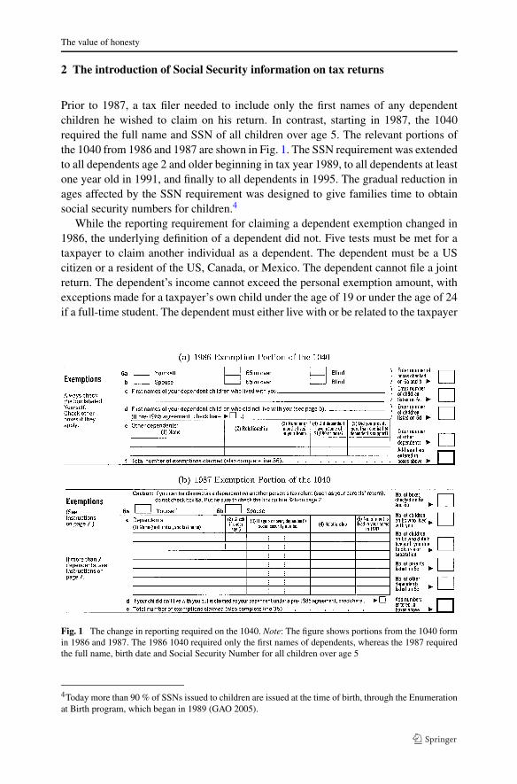
Prior to 1987, a tax filer needed to include only the first names of any dependentchildren he wished to claim on his return. In contrast, starting in 1987, the 1040required the full name and SSN of all children over age 5. The relevant portions ofthe 1040 from 1986 and 1987 are shown in Fig. 1. The SSN requirement was extendedto all dependents age 2 and older beginning in tax year 1989, to all dependents at leastone year old in 1991, and finally to all dependents in 1995. The gradual reduction inages affected by the SSN requirement was designed to give families time to obtainsocial security numbers for children.4
While the reporting requirement for claiming a dependent exemption changed in1986, the underlying definition of a dependent did not. Five tests must be met for ataxpayer to claim another individual as a dependent. The dependent must be a UScitizen or a resident of the US, Canada, or Mexico. The dependent cannot file a jointreturn. The dependent’s income cannot exceed the personal exemption amount, withexceptions made for a taxpayer’s own child under the age of 19 or under the age of 24if a full-time student. The dependent must either live with or be related to the taxpayer
Fig. 1 The change in reporting required on the 1040. Note: The figure shows portions from the 1040 formin 1986 and 1987. The 1986 1040 required only the first names of dependents, whereas the 1987 requiredthe full name, birth date and Social Security Number for all children over age 5
4Today more than 90 % of SSNs issued to children are issued at the time of birth, through the Enumerationat Birth program, which began in 1989 (GAO 2005).

S. LaLumia, J.M. Sallee
claiming her. Finally, more than half of the dependent’s support must be provided bythe taxpayer claiming her. None of these tests changed between 1986 and 1987.5
The Tax Reform Act of 1986 did make changes that may have influenced thedependent status of some individuals. Prior to the reform, a child who was claimed asa dependent by his parents but who also filed his own return could claim a personalexemption for himself. This “double-dipping” was eliminated by TRA86. Beginningin 1987, dependents were not permitted to claim a personal exemption and in mostcases could claim only a limited standard deduction. This may have created somenegotiation between parents and children about how long to remain a dependent.6
The value to parents of claiming an additional exemption also changed in 1986. Thenominal value of a personal exemption rose from $1080 to $1900 while marginal taxrates fell for most taxpayers. We return to these changes below when interpreting ourdata.
3 Tax return panel data
We use data from the University of Michigan tax panel, compiled by the Office ofTax Policy Research (OTPR). The starting point for this dataset is the annual cross-sections of tax return data released by the Statistics of Income (SOI) division of theIRS. These cross-sections report information from most lines of the tax return andfrom many supporting schedules. There is information on the total number of exemp-tions (including extra exemptions for filers who are blind or over age 65), the numberof exemptions for dependent children (reported separately for children living at homeand children living away from home), and the number of exemptions for dependentsother than children. To protect taxpayer confidentiality, income amounts are blurredand the number of exemptions is topcoded in some cases.7
Auten and Carroll (1999) describe the two methods used to select returns for inclu-sion in the annual SOI cross-sectional files. First, a nonstratified sample is drawn bychoosing certain four-digit combinations and selecting all returns on which the pri-mary filer’s SSN ends with one of these combinations. This set of randomly chosenreturns is known as the Continuous Work History Survey. Second, a stratified sample
5Recent research on dependent overclaiming focuses on the Earned Income Tax Credit (EITC). McCubbin(2000) describes data from a 1994 audit of randomly selected EITC claimants. Approximately 26 % ofEITC dollars claimed were overturned upon audit, and about 70 % of these overclaims involved an errorin claiming an EITC-qualifying child. McCubbin further finds that misclaiming a child is sensitive to thesize of the associated benefit. She estimates that a $100 increase in the tax savings from claiming a childincreases the probability of erroneously claiming an EITC-qualifying child from a mean of 8 % to 8.4 %.Liebman (2000) estimates the extent of EITC misclaiming by matching March 1991 CPS respondents to1990 tax return data. At the time, the EITC was exclusively available to filers with children. Liebmanestimates that 11 to 13 % of 1990 EITC recipients did not have a child in their CPS household as of March1991, and 10 % did not have a child in the household one year earlier.6See Whittington and Peters (1996) for evidence that the tax effect on this decision is small.7For returns with adjusted gross income (AGI) greater than $200,000, the number of exemptions for chil-dren living at home is topcoded at 3. This topcoding is unlikely to affect our results, as only 7 filing unitsobserved in both 1986 and 1987 are affected. The number of filing units affected in any other pair of yearsover which dependent loss is calculated is never greater than 22.

The value of honesty
is drawn by sorting taxpayers on the basis of level and type of income and applyingdifferent sampling rates to filers in different strata. The OTPR panel uses only thoseindividuals in the randomly selected CWHS portion of the SOI cross-sections (Slem-rod 1992), and thus the panel does not oversample high-income returns. The numberof four-digit combinations included in the CWHS sample changed over time, due toIRS budget constraints. This results in variation in the number of tax returns includedin the panel in different years. The number of tax filing units present in all 12 yearsof the panel is 4,982, and the number present in both 1986 and 1987 is 9,099.
Christian and Frischmann (1989) analyze attrition from the OTPR panel. They findthat younger, unmarried, and lower-income individuals are somewhat more likelyto drop out of the panel. A change in marital status may cause an individual to bedropped from the panel, as only the SSN of the primary filer is used in linking returnsacross years. Because men are more likely to be listed as primary filers, men havelower rates of attrition from the tax panel.8 The unbalanced nature of our panel leadsus to use somewhat different samples for different parts of our analysis, which wedetail in the relevant sections below.
4 Many people cheated on their tax returns
Our tax panel data allow us to look at the number of filers who lose net dependentseach year by comparing the number of dependents in one year against the numberclaimed the following year. If many filers were cheating up until 1986, then we wouldexpect to see a large number of filers losing dependents in 1987. Figure 2 plots thepercentage of filers who lost at least one dependent in each year of our panel, con-ditional on claiming a dependent in the previous year. There is a dramatic spike in1987, when 20.3 % of filers lost a dependent, compared to an average of 14.0 % inall other years.9 If the 1987 surge in dependent losses is entirely due to cheating, thenapproximately 31 % ((20.3 − 14)/20.3) of the 1987 dependent losers are cheaters.The number of “excess” dependent-losing filers in 1987 is equal to 2.5 % of the filingpopulation. Figure 2 also plots the fraction of filers who gain at least one dependentin each year, which shows no commensurate change between 1986 and 1987.10 Somecheaters may have chosen to claim more than one fictitious dependent. The percent-age of filers losing multiple dependents is 4.4 % in 1987, substantially greater than
8Because children are more likely to live with unmarried mothers than unmarried fathers, estimates of thetotal number of dependents from the tax panel are somewhat lower than the total number of dependentsappearing in cross-sections of tax return data. This gap is visible in Fig. 3 below.9There are other cases in which requiring a taxpayer to provide a straightforward piece of supportingevidence has generated a large change in reporting. Fack and Landais (2011) show that when Francefirst required that receipts for charitable contributions be submitted with tax returns, reported charitablecontributions fell by 75 %.10Note that the shares losing and gaining dependents are calculated with different bases in Fig. 2. All filersobserved in two consecutive years are included when computing the share of filers gaining a dependent.Only filers observed in two consecutive years and claiming a dependent in the first year are included whencomputing the share losing a dependent. If we compute the share losing a dependent without conditioningon previously claiming one, 1987 still stands out. About 8 % of filing units lose a dependent in 1987,compared to 5 to 6 % in all other years.

S. LaLumia, J.M. Sallee
Fig. 2 Percentage of tax filers who lose and gain at least one dependent each year. Note: Estimates arethe authors’ calculations from OTPR data. Dependent exemptions claimed includ exemptions for childrenliving at home, children living away from home, parents, and other dependents. In computing the share ofreturns losing dependents in year t , the denominator is the set of filing units observed in both t and t − 1claiming a positive number of dependent exemptions in t − 1. In computing the share of returns gainingdependents in year t , the denominator is all filing units observed in both t and t − 1
the 2.2 % to 2.9 % losing multiple dependents in any other year of the panel. We viewthis as further evidence of cheating, but throughout we focus on the decision to claima marginal extra dependent.
The percentage of filers losing a dependent is already a bit higher than its long-runaverage in 1986. The Tax Reform Act was passed in October 1986, several monthsbefore tax returns were due, and the 1986 instruction booklet included informationabout the upcoming SSN requirements. If the slight uptick in losses in 1986 was dueto anticipation of the reform by cheaters, then our calculation will underestimate thenumber of cheaters. It is clear from the figure, however, that any anticipatory effectis a small fraction of the total.
We can also compare the number of child dependents claimed on tax returns tothe number of children in the population from census estimates, which we do inFig. 3. Our tax data do not include the age of dependents, so we cannot perfectlymatch tax-based and census-based counts by age. Instead, we plot the ratio of alldependents to the total population under 19 and under 24. Dependents who meet thecitizenship, joint return, residency, and support tests can be claimed as a dependentirrespective of their income if they are below age 19, or if they are full-time studentsunder age 24. The majority of children under 19 will be claimed as dependents, andchildren of any age can be claimed if they have sufficiently low income and meetthe other requirements. Children of nonfilers, however, will not appear on any return,so it is ambiguous whether we expect the total dependents claimed to be larger orsmaller than these population bases. Our interest, however, is not in the ratio itself,but in whether or not the ratio changes suddenly in 1987.
Panel (a) of Fig. 3 shows the ratio of the number of child dependent exemptionsclaimed (for children living at home and children living away from home) to the num-

The value of honesty
Fig. 3 Number of dependents claimed. In panel (a) estimates of the population under 19 and under 24come from the United States Census Bureau. In both panels, estimates of the number of child dependentsclaimed on tax returns (including children living at home and children living away from home) come fromthe authors’ calculations of OTPR data (labeled OTPR Panel) and IRS publication 1304 (labeled AggregateData)
ber of children under age 19 and to the number of children under age 24.11 The figureshows both our calculations using the OTPR tax panel and aggregate totals reportedby the IRS in publication 1304.12 These data show that the relationship between thenumber of child dependents and the number of children in the population was quitesteady in the early years of our analysis.13 This is true whether the denominator isthe population of children under 19 (the upper lines in the figure) or the populationof children under 24 (lower lines), and whether the dependents are measured with theOTPR data (solid lines) or the IRS aggregates (dashed lines). In 1987, there was asignificant fall in the number of dependents that does not correspond to any changein the underlying population. This pattern is striking: it is consistent across all fourseries, and it correlates exactly with the increase in dependent losses shown in Fig. 2.
The Tax Reform Act of 1986 increased the value of the standard deduction and thepersonal exemption, which increased the income at which a person is required to filea tax return. This could cause some low-income children to disappear from tax data.The coincident expansion of the EITC, however, will have worked in the oppositedirection. Given these changes, it is useful to look also at the number of dependentsclaimed per return. In panel (b) of Fig. 3, we plot the ratio of the total number ofdependents claimed to the total number of tax returns filed, using both OTPR panel
11The previous figure includes all dependents claimed, regardless of their relationship to the filer. Thisfigure considers only dependents who are children of filers. Children account for 95 % of all dependentsclaimed. All returns observed in the OTPR panel in a given year are used to estimate the total number ofchild dependents, with different weights across years to account for the fluctuations in sample size.12We thank Brian Erard for providing us with the publication 1304 data. Despite the small size of theOTPR panel, the values we impute from it are a close match to values computed from aggregate data.13The slight increase over time in both series is consistent with rising college enrollment rates, whichenables more children between 19 and 24 to be claimed. Data from the National Center for EducationStatistics (1995) show that the college enrollment rate of 18- to 24-year olds increased from 25 % in 1979to 28 % in 1986.

S. LaLumia, J.M. Sallee
and SOI aggregate data. Both data sources indicate a sharp decline in dependentsclaimed in 1987, with no subsequent recovery.
A simple estimate of the number of inappropriate dependent claims can be derivedunder the assumption that filers lost more dependents in 1987 than in other yearssolely because many people were cheating prior to the reform, but stopped cheatingin 1987. Under that assumption, the “extra” dependent losses observed in the panelbetween 1986 and 1987 correspond to 4.2 million improperly claimed dependents,or 5.5 % of all dependents claimed in 1986. The original IRS report suggested thatthe decline in dependents was equal to 7 million, based on the difference between aforecast of 76.7 million dependents and an actual number of 69.7 (Szilagyi 1990). Thereport does not, however, explain the nature of the forecast, and the citation for theactual number says simply “SOI data.” SOI publication 1304 tables show the actualnumber of dependents claimed was 77.1 million in 1986 and 71.9 million in 1987,suggesting a decline of 5.2 million dependents. Our estimate of 4.2 million treats allexcess dependent losses as cheating, but does not count any anticipatory changes thatoccurred in 1986, nor does it include anyone who continued to cheat in spite of thereform. Attributing the 1986 uptick in dependent losses wholly to the reform wouldraise this estimate to 5. Thus, estimates from the OTPR panel are broadly consistentwith the decline documented elsewhere, though they are somewhat smaller than theoriginal number reported in Szilagyi (1990), which we suspect was too high.
The policy reform in 1987 only required an SSN for children aged 5 and above. In1989, the law required an SSN for children over the age of 2. Thus, in 1987, a devotedtax evader could have gained two more years of fake dependent claims by stating thattheir dependents were under 5. This would then lead to a drop in dependents claimedin 1989. In Fig. 2 we do not, however, see any evidence of extra “lost” dependents in1989. (There are additional changes in 1991 and 1995, but these are outside the timespan of our data.) Why not? Even though an SSN was not required for children underage 5, the 1987 form 1040 did require the dependent’s full name and relationship tothe filer for younger children, whereas it had previously required only the first nameof dependent children (see Fig. 1). While the SSN is what enables the IRS to easilyverify identity, the additional information required for all children made it more likelythat the IRS could detect cheating, even for younger children. Moreover, taxpayersmay have interpreted the change as indicating a broader effort to crack down on theinappropriate claiming of dependents.
It is also possible that the staunchest cheaters continued cheating through the 1989change. If a cheater was willing to claim that a false dependent was under the age of5 in 1987, he may have been bold enough to claim a new dependent under the age of2 in 1989, or to write in a false SSN.14 In sum, while it is plausible to have expectedsome decline in cheating in 1989, it is not necessarily surprising that any such changeis too small to show up in the data.
14Using a fake SSN may have been a viable strategy because the IRS, lacking resources, only computermatched 3 % of SSNs in the years just after the change (General Accounting Office 1993).

The value of honesty
4.1 Could the change in dependents be due to those lacking SSNs?
The 1987 reform required that filers record the social security number of dependentsto be claimed. While it is now common for an SSN to be issued at the time of achild’s birth, this was not standard practice in 1987. Instead, some children were firstassigned an SSN when their parents established a savings account for them or whenthey first entered the labor market. Could the sharp decrease in dependents be due tomany legitimate dependents who lacked an SSN being left off of returns?
Several factors weigh against this explanation. First, the SSN application for achild was not particularly arduous. To apply, parents needed to submit a one-pageform, the SS-5, along with proof of age, citizenship, and identity to the Social Se-curity Administration. The form, which could be submitted by mail, was referencedin the 1987 1040 instruction booklet, and it was widely available in post offices, li-braries, and other places where tax forms were distributed. A certified copy of a birthcertificate was sufficient to establish both age and citizenship, and medical, school,or day care records could be used to establish identity. Applications were typicallyprocessed within 10 to 14 days (New York Amsterdam News 1988).
Second, the need for an SSN was well publicized before the requirement becameeffective. The law was passed in October of 1986, 18 months before the relevant filingdeadline of April 15, 1988. In the fall of 1987, the IRS sent a mass mailing to 90million taxpayers that highlighted the new SSN requirement and other major reforms(Los Angeles Times 1987). The upcoming SSN requirement was also described in theinstruction booklet for 1986 returns, which would have given many filers advancednotice.
Even though the SSN requirement was announced long in advance of its imple-mentation, was well publicized, and involved a straightforward and quick applicationprocess, some parents may still have been unaware of the requirement or may haveprocrastinated until it was time to file their taxes. Nevertheless, parents who had notobtained an SSN on time could still claim their children. The 1040 instruction book-let directed such parents to immediately apply for an SSN and to write “Applied For”on the corresponding line of the 1040. Thus, while recent research has demonstratedthat procrastination and inertia can lead taxpayers to forego tax value by not optimallytiming withholding (Jones 2012), we think this is of little concern here, both becausethe amount of money at stake is large and because parents had the option to apply foran SSN even after filing. Moreover, low-income families, whom we might suspectof facing the largest barriers to obtaining an SSN on time, likely already had SSNsfor their children because all recipients of AFDC and Medicaid had been required tohave SSNs since 1972 (Long 1993).
To further explore this issue, we analyzed data provided in Long (1993) on thenumber of new SSNs issued for three age categories: under 1, between 1 and 4, andbetween 5 and 16. If the decline in dependents claimed in 1987 was due to legitimatedependents who lacked SSNs, but later received them, then we would expect to see arise in the number of SSNs issued to children above age 5 (the affected category in1987) for several years after the reform. Alternatively, if nearly all legitimate depen-dents over age 5 obtained an SSN in order to be claimed on their 1987 tax returns,we would expect to see a surge in calendar year 1987 and 1988 issuances, followedby a return to prereform levels.

S. LaLumia, J.M. Sallee
Fig. 4 Number of SSNs issued,by age of applicant. Note: dataare from Long (1993)
The data are shown in Fig. 4. Prior to 1987, the number of SSNs issued is very sta-ble in all three age categories shown.15 There is then a tripling of claims for childrenover age 5 in the next 2 years, after which the series returns to the prereform level andbegins to decline. The decline is consistent with the increase in issuances for youngerage categories that began in 1987, which would leave fewer children in the older cat-egory in need of an SSN in the later years. These other age categories are similarlyresponsive to the tax law. The SSN requirement was extended to children ages 1 to4 in tax year 1989, which led to a jump in issuances for that category in 1989 and1990, despite downward pressure from the rise in newborn issuances. Overall, thedata closely follow the pattern predicted by parents promptly obtaining an SSN assoon as it is required for tax purposes. The IRS itself was concerned with this issueand concluded that SSNs were not a significant barrier to legitimate claiming. Theyconducted surveys showing that, among taxpayers with children ages 5 and older, theshare with SSNs for their children rose from 67 % in May 1987 to 89 % in January1988—still several months before the 1987 filing deadline (Szilagyi 1990).
Finally, if failure to obtain an SSN prevented parents of legitimate dependentsfrom claiming them in 1987, we would expect to see a disproportionate number ofthose filers gaining a dependent in subsequent periods, once they had obtained anumber. To examine this possibility, we use our OTPR panel data to plot the fractionof filers who gain a dependent, conditional on having lost a dependent in a particularyear, in Fig. 5. Each line in the figure represents those who lost a dependent in adifferent year, with 1987 in bold, and each data point shows the fraction who gain adependent t years before or after a loss. Because our panel is unbalanced, the sampleused in each data point differs slightly. To be included, a taxpayer had to file in boththe base year and the year before that (in order to determine if they lost a dependent inthe base year), as well as the relative year shown and the year before that (in order to
15There is a noticeable uptick in SSN applications in 1983. This is the first year in which recipientsof interest and dividend payments needed to provide an SSN to the financial institution issuing thesepayments (Long 1993). Parents who had established savings accounts in the names of their children wouldhave needed SSNs for their children at this point.

The value of honesty
Fig. 5 Share gaining adependent, among those losingdependent in year 0. Note: Eachline in the figure corresponds toa different subsample from theOTPR panel: the set of filingunits losing at least onedependent in a particular year.The bold line corresponds to the721 filing units observed losingat least one dependent in 1987.We follow each sample overtime, computing the share ofthese filing units gaining adependent in each earlier andlater year
determine if they gained a dependent). For example, the year 1 value for the sampleshown in bold is calculated over filers observed in 1988 as well as 1986 and 1987.The year 3 value for the sample shown in bold is calculated over filers observed in1986 and 1987 (allowing identification of a dependent loss in 1987) as well as in1989 and 1990 (allowing identification of a dependent gain in 1990).16
The data show considerable churning. Relative to year zero (when a filer lost a de-pendent), filers are relatively likely to have gained a dependent immediately before orafter that loss. This is true in every year, not just 1987.17 If many filers lost a depen-dent in 1987 because of missing SSNs, we would have expected a large increase independent gains for those filers in subsequent years, relative to the gain experiencedby filers who lost dependents in non-reform years. This is not the case; 1987 appearstypical. If anything, gains are low immediately after 1987 losses, which is consis-tent with cheaters being less likely than legitimate losers of dependents to regain thedependent in the subsequent year.18
We cannot definitively eliminate the possibility that missing SSNs account forsome of the decline in dependents in 1987. If there were some such cases, our es-timates may overstate cheating. But, the administrative details, the pattern of SSNissuances, and the lack of a dramatic deviation in regaining suggest that this plays atmost a minor role.
16Because underlying fluctuations in the sample may be affecting the patterns we observe, we have con-structed a balanced-panel version of Fig. 5 that includes only those filing units observed in all years of thepanel. This alternative figure is quite similar; it too shows that the group of filers who lose dependents in1987 is not particularly likely to gain dependents in subsequent years.17This may result in part from changes in who is claiming dependents following marital changes. In caseswhere a filing unit loses a dependent and gains a dependent in the following year, 25.3 % transitioned outof married filing jointly status at some earlier point in the panel. Among filing units losing a dependentin one year and not subsequently regaining, only 14.7 % had previously transitioned out of married filingjointly status.18In the extreme case where cheaters have a zero chance of regaining a dependent, however, we wouldexpect to see an even lower rate of regaining for 1987 dependent losers, given that nearly one-third ofthis group are estimated to be cheaters. This suggests that there could be modestly higher than averageregaining rates among honest filers who lost a dependent in 1987.

S. LaLumia, J.M. Sallee
4.2 Could the change in dependents be due to other changes in TRA86?
The Tax Reform Act of 1986 involved many other tax changes. Could any of these bethe source of a large reduction in dependents? The most obvious feature of TRA86relevant here is a change in the tax treatment of dependent filers. Prior to 1986, a childwho filed his own return could claim a personal exemption on his return and still beclaimed as a dependent by his parents. After 1987, this was not allowed, so childrenand parents had to choose whether the child would file with zero exemptions, and al-low the parents to claim the exemption, or vice versa. If many families chose to allowincome-earning children, who qualified as dependents, to claim themselves insteadof claiming them as dependents on the parents’ returns, then this could generate aone-time drop in dependents claimed in 1987.
In a tax-minimizing household, a child will claim an exemption for herself onlywhen her tax savings from the exemption exceed the parents’ tax savings from claim-ing an additional dependent.19 The value of the exemption depends entirely on themarginal tax rate. For it to be tax-minimizing for a child to claim herself, that childwould need to earn sufficiently more money than her parents so as to be in a highertax bracket, and yet still live in her parents’ home and obtain more than 50 % of herfinancial support from her parents, so as to qualify as a dependent.
Such arrangements are rare, as is shown in Table 1, which uses March CurrentPopulation Survey (CPS) data from 1987. We constructed a sample of children, be-
Table 1 Children’s income relative to parents’ income
Full sample Ages 15–18 Ages 19–23
A. Wage income
% with any 54.7 47.6 77.8
Mean amount 1,317 836 2,883
% with wages > 0.75· parents’ wages 6.2 5.5 8.5
% with wages > parents’ wages 5.7 5.1 7.3
Median of (own wages/parents’ wages) 0.007 0 0.049
B. Total income
% with any 66.2 59.8 86.9
Mean amount 1,874 1,229 3,977
% with inc. > 0.75· parents’ inc. 2.8 2.5 3.6
% with inc. > parents’ inc. 2.0 1.8 2.6
Median of (own inc./parents’ inc.) 0.015 0.005 0.068
N 11,369 8,853 2,516
Data are from the March 1987 CPS. Sample is restricted to children of household heads and to those eitherbetween the ages of 15 and 18 or between the ages of 19 and 23 and enrolled in school full-time
19A caveat here is that households may fail to minimize taxes in this manner under models of intrahouse-hold bargaining that lead to inefficiencies. A unitary household model, a model that results in efficientbargaining, or one that includes transferable utility will result in tax minimization because these modelspredict that families will maximize welfare and then bargain over the surplus.

The value of honesty
tween the ages of 15 and 23, living with one or both parents. The lower age cutoffreflects the fact that only individuals aged 15 or older report income information inthe CPS. All children between ages 15 and 18 are included, while children betweenages 19 and 23 are included only if they are full-time students. Table 1 shows that66.2 % of these potential dependents had some form of income, and 54.7 % had wageincome. Not surprisingly, the median ratio of a child’s income to his parents’ incomeis 0.015. Only 2.8 % of children had income equal to 75 % of their parents’ income,and just 2 % had income equal to or greater than their parents’. In sum, given the lowprobability that it would have been tax-minimizing for children to claim themselves,we expect that this aspect of the 1986 reform is unlikely to explain an importantfraction of the drop in dependents.
5 Many other people paid to be honest
Our data suggest that around 2.5 % of taxpayers were cheating by improperly claim-ing dependents in 1986. Conversely, this means that 97.5 % were not cheating. Thisis perhaps the more surprising statistic, given the substantial amount of income thatcould have been taken at relatively low risk by claiming fraudulent dependents. Im-portantly, the 97.5 % of taxpayers who did not avail themselves of this opportunity tocheat implicitly demonstrated that they would rather give up several hundred dollarsin income than cheat the government. Overall, we think this is striking evidence of abroad willingness to pay to be honest across the taxpayer base.
How much did honest taxpayers forego? To answer this question, we would like toeliminate the tax cheaters from the sample and tabulate the tax savings from claimingan extra dependent that would have been enjoyed by the honest taxpayers had theycheated. Unfortunately, there is no way to directly identify the cheaters in the data.We can, however, identify groups of filers who were almost certainly honest. Onesuch group is the set of filers who did not lose a dependent between 1986 and 1987,who make up 92 % of filers, whom we analyze in Table 2.
Table 2 shows the average 1986 tax savings associated with the marginal depen-dent for filers who appear in the panel in both 1986 and 1987. These statistics areobtained by comparing the after-tax income of filers given the actual number of de-pendents reported in the data against their hypothetical after-tax income when theyhave one additional (or one fewer) dependent, as calculated by TAXSIM.20 The after-tax income gain that would have accrued to families from claiming one additionalchild represents the gain to be had from cheating. On average, those who did not losea dependent between 1986 and 1987 would have saved $275 on their 1986 taxes byclaiming an additional dependent. The mean savings is even higher, $291, for thosewho claimed zero dependents. We view both of these groups as consisting of honesttaxpayers. These savings are in 1986 dollars; inflating by the CPI to 2010 dollarsdoubles the estimates to $547 and $579.21
20The TAXSIM program is described by Feenberg and Coutts (1993).21We use the CPI-U all items, which was 109.6 in 1986 and almost exactly double, 218.1, in 2010.

S. LaLumia, J.M. Sallee
Table 2 The value of claiming a dependent
N Gain fromadditionaldep., 1986
Loss fromone fewerdep., 1986
After-taxincome
Taxliability
Observed in 86 and 87 9,099 271 22,006 3,898
(160) (28,108) (16,573)
No deps. in 1986 5,548 291 17,878 3,509
(176) (27,030) (18,081)
Deps. in 1986 3,551 239 −271 28,457 4,505
(123) (126) (28,546) (13,875)
Lost dep. in 1987 721 224 −254 25,868 3,943
(121) (127) (25,888) (11,082)
Did not lose in 1987 2,830 243 −276 29,117 4,648
(123) (126) (29,152) (14,499)Did not lose dep. in1987
8,378 275 21,674 3,894
(162) (28,268) (16,964)
Calculations of the gain (loss) associated with claiming one additional (fewer) dependent rely on TAXSIMestimates of tax liability, using income elements and household composition reported on 1986 tax returns.Standard deviations are in parentheses. After-tax income is defined as AGI minus total income tax liability,as reported on 1986 tax returns
Fig. 6 Value of claiming oneadditional dependent, nonlosers,1986. Note: Figure plots thedifference between twoTAXSIM computed taxliabilities for each filing unit, forunits that appear in both 1986and 1987 and do not lose adependent. The first value is thetax liability that results fromapplying 1986 tax law to actualreported 1986 income anddependent exemptions. Thesecond value adds one to thenumber of dependents claimed
Figure 6 shows the distribution of tax savings that would have accrued to filers ifthey had claimed an additional dependent in 1986, for the sample of returns that didnot lose dependents between 1986 and 1987 (and are therefore assumed to be honestpayers). Dependent exemptions are nonrefundable, so claiming an additional depen-dent has zero impact for low-liability filers. Among those not losing a dependentbetween 1986 and 1987, 7.3 % would have gained nothing. The average tax savingsfrom an additional dependent among the remaining filers was larger. In this sampleof presumably honest taxpayers, 69.4 % stood to gain at least $200, and 18.0 % stoodto gain at least $400 by claiming an extra dependent.
The value of honesty
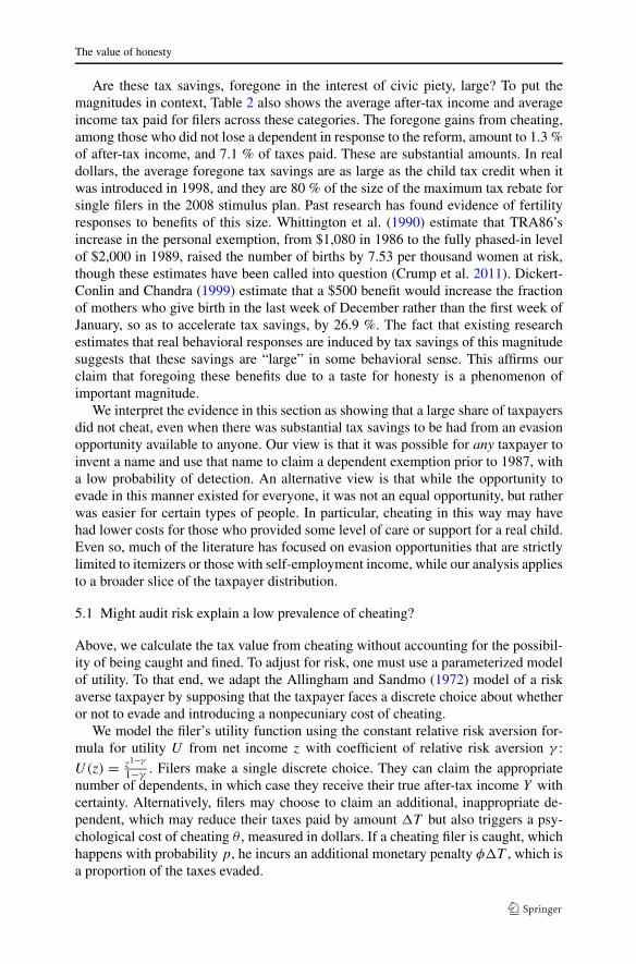
Are these tax savings, foregone in the interest of civic piety, large? To put themagnitudes in context, Table 2 also shows the average after-tax income and averageincome tax paid for filers across these categories. The foregone gains from cheating,among those who did not lose a dependent in response to the reform, amount to 1.3 %of after-tax income, and 7.1 % of taxes paid. These are substantial amounts. In realdollars, the average foregone tax savings are as large as the child tax credit when itwas introduced in 1998, and they are 80 % of the size of the maximum tax rebate forsingle filers in the 2008 stimulus plan. Past research has found evidence of fertilityresponses to benefits of this size. Whittington et al. (1990) estimate that TRA86’sincrease in the personal exemption, from $1,080 in 1986 to the fully phased-in levelof $2,000 in 1989, raised the number of births by 7.53 per thousand women at risk,though these estimates have been called into question (Crump et al. 2011). Dickert-Conlin and Chandra (1999) estimate that a $500 benefit would increase the fractionof mothers who give birth in the last week of December rather than the first week ofJanuary, so as to accelerate tax savings, by 26.9 %. The fact that existing researchestimates that real behavioral responses are induced by tax savings of this magnitudesuggests that these savings are “large” in some behavioral sense. This affirms ourclaim that foregoing these benefits due to a taste for honesty is a phenomenon ofimportant magnitude.
We interpret the evidence in this section as showing that a large share of taxpayersdid not cheat, even when there was substantial tax savings to be had from an evasionopportunity available to anyone. Our view is that it was possible for any taxpayer toinvent a name and use that name to claim a dependent exemption prior to 1987, witha low probability of detection. An alternative view is that while the opportunity toevade in this manner existed for everyone, it was not an equal opportunity, but ratherwas easier for certain types of people. In particular, cheating in this way may havehad lower costs for those who provided some level of care or support for a real child.Even so, much of the literature has focused on evasion opportunities that are strictlylimited to itemizers or those with self-employment income, while our analysis appliesto a broader slice of the taxpayer distribution.
5.1 Might audit risk explain a low prevalence of cheating?
Above, we calculate the tax value from cheating without accounting for the possibil-ity of being caught and fined. To adjust for risk, one must use a parameterized modelof utility. To that end, we adapt the Allingham and Sandmo (1972) model of a riskaverse taxpayer by supposing that the taxpayer faces a discrete choice about whetheror not to evade and introducing a nonpecuniary cost of cheating.
We model the filer’s utility function using the constant relative risk aversion for-mula for utility U from net income z with coefficient of relative risk aversion γ :
U(z) = z1−γ
1−γ. Filers make a single discrete choice. They can claim the appropriate
number of dependents, in which case they receive their true after-tax income Y withcertainty. Alternatively, filers may choose to claim an additional, inappropriate de-pendent, which may reduce their taxes paid by amount �T but also triggers a psy-chological cost of cheating θ , measured in dollars. If a cheating filer is caught, whichhappens with probability p, he incurs an additional monetary penalty φ�T , which isa proportion of the taxes evaded.

S. LaLumia, J.M. Sallee
In this model, an individual i will cheat if and only if:
(1 − p)(Yi + �Ti − θi)
1−γ
1 − γ+ p
(Yi − φ�Ti − θi)1−γ
1 − γ>
Y1−γ
i
1 − γ, (1)
which says simply that the individual will evade when the expected payoff to cheat-ing is greater than the expected payoff to being honest. For any given set of parametervalues, there will be some value of θ , call it θ∗, that would make the taxpayer indif-ferent. If θi is greater than θ∗, then person i will not evade because the psychologicalcost makes honesty preferable.
This parameterization is useful in allowing us to estimate the quantitative impor-tance of risk and in providing a precise definition of the honesty premium we describeabove. Our calculations above, which show the amount of money foregone by an hon-est taxpayer, can be interpreted as saying that for any individual i who chooses to behonest, their θi is greater than the foregone tax savings we calculate. When evasionis a discrete choice, what we estimate from observing an honest taxpayer is a lowerbound on his willingness to pay to be honest.
To parameterize our model, we substitute in values for income, tax savings, proba-bility of audit, evasion penalties, and risk aversion. Then we calculate the value of θ∗,which tells us the psychological aversion to cheating that would make an individualindifferent to evasion given the other values. If this number is close to the nominaltax savings, then it implies that risk has little impact on the calculation, and that thenominal tax savings we presented above are good estimates of a lower bound on thepsychological aversion to cheating. For heuristic value, we also assume that θ = 0,that there is no willingness to pay to be honest, and calculate the probability of auditrequired to make an individual indifferent to cheating, labeled p∗. With no honestypremium, an individual will cheat if they believe p to be below p∗.
Table 3 presents results for four scenarios. For Y , we use $21,670, the mean after-tax income in our 1986 sample of filers who did not lose a dependent in 1987. Taxsavings �T is set equal to the mean in our sample for these filers, $275. The fractionof tax returns audited in 1986 was around 2 %, so we set p = 0.02 as our probabilityof detection.22 We set γ = 2, which is close to estimates in Chetty (2006) and Attana-sio and Paiella (2011). There are two classes of penalties for underpayment of taxes.Any part of underpayment due to “negligence or disregard of rules or regulations”is subject to a 20 % penalty, while any part of underpayment attributable to fraudis subject to a 75 % penalty. If taxpayers can claim plausible confusion about theirmispayment, they will pay the 20 % rate, which applies to the vast majority of cases.We use this as our baseline, so φ = 0.2. Throughout this exercise, we assume filersare not cheating in any way other than misclaiming a dependent.23
22Between 1977 and 1986, the audit rate gradually fell from 1.88 % to 1 % (Dubin et al. 1990). Between1988 and 1995, the audit rate ranged between values of 0.92 % and 1.67 % (General Accounting Office1996).23If filers are cheating on other margins, this creates background risk, which will have a small effect onour calculations. The effect is small because this other risk is born whether the individual decides to claima false dependent or not. So long as the probability of audit is not a function of claiming a false dependent

The value of honesty
Table 3 Sample values of the role of risk
Y �T γ p φ θ∗ p∗
21,670 275 2 0.02 0.2 268 0.83
21,670 275 2 0.02 0.75 265 0.57
21,670 275 10 0.02 0.75 264 0.54
21,670 275 10 0.20 0.75 170 0.54
Table shows pretax income Y , the change in taxes paid from evasion �T , the coefficient of absolute riskaversion γ , the probability of audit p, the IRS penalty as a fraction of taxes evaded φ, the break-evenwillingness to pay to be honest, which makes a taxpayer indifferent between cheating and not θ∗ , and theprobability of audit that would make the taxpayer indifferent between cheating and not if θ = 0, p∗
The first row of Table 3 shows our baseline estimates. An individual who couldsave $275 in taxes by improperly claiming a dependent would be willing to do so aslong as his psychological cost of cheating is below $268. This suggests that, for ourbaseline parameters, risk is not an important explanation for why so many taxpayersfailed to cheat. Another way to see this is to calculate the probability of audit thatwould make a filer indifferent between cheating and not cheating (p∗), assumingθ = 0. For our baseline case, that break-even probability is an extremely high 83 %:If the taxpayer has no aversion to cheating (θ = 0), then he has to believe that theprobability of audit is at least 83 % to not cheat.
For robustness, we vary the risk coefficient γ , the probability of audit p, andthe penalty fraction φ. We show a subset of representative results in Table 3. Theonly parameter that substantially changes the value of cheating is the probability ofaudit.24 Combined with high risk aversion and criminal penalties, if filers believe theprobability of being caught is 20 %, instead of 2 %, then the payoff to a nominal$275 of savings falls to $170. Even higher audit probabilities further erode the valueof cheating, but they must be above 50 % for cheating to become a net negativeproposition when θ = 0, even with high penalties and risk aversion.
Might taxpayers believe the probability of audit is extremely high? Coarse infor-mation about perceived audit probabilities is available from the 1987 Taxpayer Opin-ion Survey. When asked about the likelihood of their 1986 returns being audited,35 % of respondents said it was not very likely, 42 % said it was highly unlikely, andanother 15 % were not sure.
This framework formalizes the economic interpretation of our data from the 1986reform. Those people who did not cheat must have a θi ≥ θ∗, where θ∗ will beroughly 97.5 % of the estimated tax savings in Table 2 for our base case, and wellover 90 % for even the most extreme scenarios, unless taxfilers believe their proba-
(which is likely because so many people claim dependents that this cannot be a useful audit criterion), oursimplification is an important restriction only if falsely claiming a dependent makes other cheating easierto detect, conditional on audit.24Estimates of the coefficient of relative risk aversion based on observed equity return premiums are in theneighborhood of 50 (DeLong and Magin 2009). Even numbers in this range have almost no impact on ourestimates.

S. LaLumia, J.M. Sallee
bility of being caught is much higher than the actual audit rates. Based on this, weconclude that the taste for honesty is substantial, even accounting for risk.25
5.2 Might ignorance explain a low prevalence of cheating?
An alternative interpretation is that filers who did not claim fictitious dependentsprior to the reform were not doing so out of love of country, but instead because theopportunity to cheat had simply never occurred to them. Unfortunately, there is noway to directly measure the number of people who lacked the cleverness to cheat.That said, this evasion opportunity is very simple and easy. The box for dependentsclaimed is right at the top of the 1040, as shown in Fig. 1. Moreover, if filers do nothave a distaste for cheating, then we would expect them to invest effort in searchingfor low-hanging evasion fruit, like the dependent exemption. If filers were ignorantbecause they had no intention of cheating and, therefore, did not look for easy ways tocheat, then this is a round about way of affirming our hypothesis that they are willingto pay to be honest.
We suspect that people who claimed dependents at some point in time, and partic-ularly those who had a change in the number of dependents, are aware of the tax valueof dependents and the ease of claiming them. For filers who appear in all years of thetax panel, 66 % had a dependent at some point in time, and 59 % have a changein the number of dependents claimed during the sample period. Narrowing in on agroup likely to be honest, filers who do not lose a dependent between 1986 and 1987,34 % are claiming a dependent, and 32 % had changed the number of dependentsbefore 1986. This suggests that there is a substantial opportunity to learn about thepotential gains from claiming dependents and the relative ease of doing so.
In sum, there is no way to know whether any particular individual who failed touse the child loophole to lower his tax bill did so out of ignorance. Moreover, it isimpossible to know what fraction of the honest taxpayers fall into that category. Itseems likely, however, that filers with a thirst for cheating would have come acrossthis possibility, particularly if they had experience with dependent exemptions, asmost taxpayers do.
6 Who cheated and why?
6.1 Cheaters have differences in tax return characteristics
Who cheated? Are cheaters different from honest payers in observable characteris-tics? To answer such questions, we would ideally like to know who cheated in pre-reform years, and compare their characteristics to honest taxpayers. Our panel dataallow us to identify those who lost a dependent in 1987, but there is no immediate
25In principle, estimates of the distribution of the willingness to pay to be honest could be estimatedby comparing the amount of cheating at different tax values, given an additional assumption about thejoint distribution of �T and θ . We pursued this empirical strategy but determined that the available taxpanel data are of insufficient sample size given the observed variation in tax values to produce meaningfulestimates.

The value of honesty
way to distinguish those who lost a dependent for legitimate reasons from cheaterswho reacted to the reform.
Fortunately, we can detect large differences in observable characteristics betweencheaters and noncheaters by looking at changes in summary statistics across treat-ment years, where the number of cheaters present in particular subsamples varieswidely and measurably. We pursue three different comparisons that use this basic ap-proach. All three combine mild distributional assumptions with estimates of the num-ber of cheaters in particular subsamples (taken from changes in observable statisticsin response to the policy reform) to uncover facts about the characteristics of cheaters.These approaches may prove useful in other contexts. Here, they are especially com-pelling because all three approaches yield similar estimates, indicating that cheaterswere more likely to be heads of household, less likely to be married filing jointly,and more likely to claim the child care credit. The main limitation to our exerciseis that we are restricted to the variables that appear on tax returns, which excludesinteresting demographics like age, education and occupation.
First, suppose that cheaters and non-cheaters have different distributions for somecharacteristic X. If the set of 1987 dependent losers includes a substantial numberof cheaters, then the value of taxpayer characteristics among those who lost a depen-dent will be different in 1987 than in earlier years. This assumes that anyone losing adependent in an earlier year must be honest.26 Specifically, the mean value of charac-teristic X among all those who lost a dependent in 1987, denoted μx , can be writtenas a weighted sum of the mean of X for cheaters μc
x and noncheaters μhx , where the
weights are equal to the probability that someone in the sample is a cheater ρ:
μx = ρμcx + (1 − ρ)μh
x. (2)
This equation can be rearranged to form an equation for the difference in meansbetween cheaters and noncheaters:
μcx − μh
x = (μx − μh
x
)/ρ. (3)
Thus, given an estimate of the pooled mean μx , the mean of honest taxpayers μhx , and
the proportion of the 1987 sample that were cheaters ρ, we can calculate an estimateof the difference in mean characteristics between cheaters and noncheaters. We havea ready estimate of μx from our sample of returns, since it is simply the mean of all1987 dependent losers. In Sect. 4 we estimated that 31 % of those losing a dependentin 1987 were cheaters, which provides an estimate of ρ.
To obtain an estimate of μhx we use the mean of characteristic X for filers re-
porting a dependent loss in an earlier year. TRA86 created many changes in the taxcode that might cause differences in observable characteristics. To avoid conflating
26Assuming that all 1986 dependent losers are honest ignores any anticipatory changes in dependent claim-ing behavior. This will be problematic if some individuals gave up improper dependent claiming in the yearthe SSN requirement was announced rather than in the following year when it was implemented. We haveaddressed this concern by instead using the filing units losing dependents in 1985 to estimate means forhonest dependent losers. The results of this analysis are quite similar to what we report in columns 1 and 3of Table 4.

S. LaLumia, J.M. Sallee
Table 4 Summary statistics for filers losing a dependent
Lost dep.in 1986
(μ̂hx )
Lost dep.in 1987(μ̂x )
Mean diff.:cheaters −honest
( ̂
μcx − μh
x )
Among 1987 losers:Lost previously?
Yes(Honest)
No(Cheaters)
(1) (2) (3) (4) (5)
% Married, year t − 1 69.9 62.3∗ −24.5 71.1 54.5∗% Head of household, year t − 1 23.3 31.1∗ 25.2 23.5 37.7∗% with change in filing status 21.1 24.7 11.6 19.0 29.6∗% with change in state 3.6 4.2 1.9 3.3 4.9
Mean dependents, year t − 1 2.1 2.3 0.6 2.1 2.4∗Mean � in number of deps. −1.2 −1.3∗ −0.3 −1.2 −1.4∗Zero dependents after loss 47.9 44.1 −12.3 47.3 41.3
Head of HH to single after loss 10.4 13.2 9.0 10.4 15.6∗Last dependent had no tax value 7.3 5.4 −6.1 3.6 7.0∗% with child care credit, year t − 1 7.8 12.8∗ 16.1 10.1 15.1∗% with EITC, year t − 1 13.1 14.8 5.5 13.4 16.1
% age 65 or older as of 1987 6.0 4.4 −5.2 4.2 4.7
% age 65 or older as of 1990 9.5 7.5 −6.5 8.0 7.0
Mean AGI ($), year t − 1 35,695 35,550 −468 40,250 31,448∗% itemizing, year t − 1 53.6 49.0 −14.8 56.5 42.3∗% contrib. IRA, year t − 1 21.7 16.5∗ −16.8 20.2 13.2∗% contrib. election fund, year t − 1 31.7 25.2∗ −21.0 21.7 28.3∗N 549 721 336 385
Dollar amounts are real 1990 dollars. An ∗ indicates that the difference between adjacent columns isstatistically significant at the 10 % level. Column 3 is the estimated difference in means between cheatersand honest taxpayers, equal to (column 2–column 1)/0.31. Column 4 is hypothesized to have a substantiallyhigher percentage of honest taxpayers than column 5, so that the sign of the difference is indicative of thedifference in means between groups
these changes with the differences between cheaters and non-cheaters, we measurethe characteristics of the 1987 dependent losers in 1986, the year prior. For consis-tency, we compute means in the year before dependent loss for the comparison groupof honest taxpayers. We present unweighted means because the OTPR panel is con-structed from a nonstratified sample.
Table 4 shows the results of this exercise. Column 1 shows the sample mean ofcharacteristics measured in 1985 for taxpayers who lost a dependent in 1986. This isour estimate of the mean characteristic for honest taxpayers who lose a dependent.Column 2 shows the mean characteristic on 1986 tax returns (before the reform), forthose taxpayers who lost a dependent in 1987 (when the reform took effect). Asterisksindicate that this value is statistically different from column 1 at the 10 % level basedon a simple comparison of means. Column 3 shows our estimate of the differencein each characteristic between cheaters and honest losers of dependents, based onEq. (3) and assuming ρ = 0.31.

The value of honesty
Column 3 of Table 4 shows that there are significant differences between cheatersand those who lost a dependent for legitimate reasons. In particular, cheaters weremuch less likely to be married filing jointly, and much more likely to file as headof household. Moreover, more cheaters experienced a change in their filing status in1987. This is driven in large part by 1986 head of household filers shifting to theless generous single filing status in 1987, though the difference is statistically im-precise. Cheaters were also much more likely to claim the child care credit, whichis a tax credit for child care expenses incurred to enable parents or guardians towork. Taken together, the evidence shows that cheaters gained not only from claimingan additional dependent exemption, but also from moving to the head of householdrate schedule and claiming (possibly fraudulent) credits for child care expenses.27
Cheaters were also less likely to contribute to an IRA and to make a contribution tothe presidential election campaign fund (which is plausibly correlated with a sense ofcivic engagement). Other characteristics fail to show a statistically significant differ-ence.28
A second, related method of identifying differences in characteristics of cheatersand honest taxpayers comes from delineating two subgroups within the set of filerswho lost a dependent in 1987. We hypothesize that having lost a dependent in yearsprior to the reform, when there was no change in the enforcement technology fordetecting misclaimed dependents, is an indication of honesty. Thus, the group ofindividuals who lost dependents in 1987 and in earlier years likely contains a highproportion of honest taxpayers. The group of individuals who lost dependents in 1987but never before likely contains a higher proportion of cheaters. Table 4 shows themeans across these two subgroups, which are of roughly equal size, in columns 4and 5. Asterisks in column 5 indicate that there is a statistically significant differenceat the 10 % level using a simple comparison of means across the two columns.
This alternative procedure shows the same qualitative results about filing status asthe analysis in columns 1–3. First-time dependent losers were less likely to be mar-ried filing jointly in 1986, and more likely to be filing as a head of household. Manymore first-time losers experienced a change of filing status in 1987. Similarly, signif-icantly more first-time losers claimed the child care credit in 1986. This alternativecomparison also suggests that differences in AGI, the fraction itemizing, the fractioncontributing to an IRA, and the fraction contributing to the election fund are statisti-
27The IRS began requiring a Social Security number or taxpayer identification number for the careprovider for anyone claiming the child care credit in 1989. As discussed in O’Neil and Lanese (1993)and cited by Slemrod and Bakija (2008, pp. 238–239), this reform was followed by a substantial increasein the number of claims of self-employment income; a response similar in spirit to what we analyze here.28We have also replicated the comparisons in columns 1 and 2 of Table 4 for every other year in our sam-ple, as a placebo test. Overall, we find that there are 21 cases where the adjacent year means are statisticallydifferent at the 10 % level, out of 137 pairwise comparisons. In only one other year (1982) is there a sta-tistical difference in the percentage of married filers, and in only two (1982 and 1989) is there a differencein share of head of household filers. Thus, we do reject equality more often than would be predicted bypure sampling variation, but the rejection is not concentrated in our variables of interest, and we believethat other tax reforms in other years will cause some statistics to differ. There are a number of significantdifferences between the groups of filers losing dependents in 1982 and in each of the adjacent years. Wesuspect this reflects the tax reform act that took effect in 1982. There are four significant differences in theIRA contribution variable, likely reflecting changes in IRA contribution rules.

S. LaLumia, J.M. Sallee
Table 5 Probit regression predicting dependent loss
Coefficient Coefficient on 1987 interaction
Married, year t − 1 −0.026 0.006
(0.031) (0.068)
Head of household, year t − 1 0.070∗∗ 0.184∗∗(0.034) (0.081)
Change in filing status 1.049∗∗∗ 0.234∗∗∗(0.025) (0.084)
Number of dependents, year t − 1 0.185∗∗∗ 0.111∗∗∗(0.006) (0.023)
Any child care credit, year t − 1 −0.543∗∗∗ 0.059
(0.028) (0.075)
Any EITC, year t − 1 −0.059∗∗∗ 0.048
(0.022) (0.086)
Age 65 or older as of 1987 0.624∗∗∗ 0.016
(0.036) (0.150)
Any IRA contribution, year t − 1 0.183∗∗∗ −0.103
(0.026) (0.075)
Real AGI, year t − 1 (1000 s) 0.0003∗∗ −0.0003
(0.0001) (0.0006)
N 55032
The sample includes filers at risk of losing a dependent between 1980 and 1987, those who claimed atleast one dependent in the previous tax year. The dependent variable is a dummy variable coded as 1 ifthe filer lost a dependent between years t − 1 and t . The omitted other marital status category containsmainly single filers and a handful of married filing separate returns. Slightly different definitions are usedto determine when a child can be claimed as a dependent and when that child allows an unmarried parent touse the head of household filing status (Holtzblatt and McCubbin 2003). This results in about 4 % of filersclaiming dependents while using single filing status. The ∗, ∗∗ and ∗∗∗ indicate statistical significance atthe 10 %, 5 %, and 1 % levels
cally different. With the exception of election fund contributions, the differences goin the same direction as in the previous comparison of cheaters and honest filers.
To address likely correlations across taxpayer characteristics, we next estimate aprobit regression predicting dependent loss. We pool filers who are observed in twoconsecutive years up to and including 1987, and restrict the sample to those claim-ing at least one dependent in the earlier year of each pair. We control for a numberof taxpayer characteristics, and interact each of these characteristics with a dummyfor 1987 observations. This allows us to test whether a given characteristic affectsthe probability of dependent loss differently in the year when many losses representcheating. The results are shown in Table 5. In this specification, only measures ofhousehold composition appear to be associated with cheating. While filing as head ofhousehold, relative to filing as a single taxpayer, is always associated with a signifi-cantly higher probability of dependent loss, this effect is larger in 1987. The same istrue for having experienced a change in filing status between the two consecutive tax

The value of honesty
years. Other characteristics appear to affect dependent loss in the same way in 1987as in earlier years. Broadly, the results corroborate our conclusions above.
Third, we use a different decomposition to infer the difference in characteristicsacross honest taxpayers and cheaters. The prior two methodologies were premisedon a comparison of taxpayers who lost a dependent at different times, under differentenforcement regimes. We can also compare filers who lost a dependent to filers whogained a dependent.29 We start by noting that the mean of some characteristic X,among those who gain a dependent (henceforth “a gainer”) in a given tax year t ,can be written as the weighted sum of the mean of that characteristic for cheatersand honest taxpayers, where the weight is the probability that a gainer in year t is acheater:
μgx,t = ρ
gt μ
g,cx,t + (
1 − ρgt
)μ
g,hx,t . (4)
Here, μgx,t is the average characteristic for gainers in year t (which is directly observ-
able), μg,cx,t is the average characteristic for gainers who are cheaters in year t , μ
g,hx,t is
the average characteristic for gainers who are honest in year t , and ρgt is the proba-
bility that a gainer is a cheater in year t . The same decomposition can be written forthose who lose a dependent (“losers”) in a given year: μl
x,t = ρlt μ
l,cx,t + (1 − ρl
t )μl,hx,t .
If we make assumptions about the stability of mean characteristics for cheaters andhonest taxpayers, then a comparison of the change in mean characteristics of gainersand losers spurred by a change in enforcement (which is observable) can be used toinfer the difference in mean characteristics of cheaters and honest types (which isnot directly observable). Specifically, we assume that cheaters have the same char-acteristic mean, in both 1986 and 1987, regardless of whether they are gainers orlosers. That is, μ
g,c
x,87 = μl,cx,87 = μ
g,c
x,86 = μl,cx,86 ≡ μc
x . We make a parallel assumption
for honest taxpayers: μg,h
x,87 = μl,hx,87 = μ
g,h
x,86 = μl,hx,86 ≡ μh
x . Under these assumptions,it is straightforward to show that the difference in the mean characteristics betweengainers and losers can be written as
μgx,t − μl
x,t = (ρ
gt − ρl
t
)(μc
x,t − μhx,t
). (5)
This same expression can be calculated for years before and after a reform thatchanges the probability that gainers and losers are cheaters in estimable ways. Writingout the difference-in-difference between characteristics of gainers and losers acrossyears ((μg
87,t − μl87,t ) − (μ
g
86,t − μl86,t )) using Eq. (5) and rearranging yields an ex-
pression for the difference in means across cheaters and honest taxpayers, our objectof interest:
μcx − μh
x = (μg
x,87 − μlx,87) − (μ
g
x,86 − μlx,86)
(ρg
87 − ρg
86) − (ρl87 − ρl
86). (6)
The left-hand side of Eq. (6) is exactly the same object as the one estimated by ourfirst method and shown in column 3 of Table 4. The numerator on the right-hand
29We are especially grateful to Damon Jones for suggesting this approach.

S. LaLumia, J.M. Sallee
side is the difference-in-difference across gainers and losers from 1986 to 1987. Eachobject in the numerator is directly observable. The denominator is the difference-in-difference in the probability that gainers and losers are cheaters between 1986 and1987. Intuitively, this inference procedure examines the difference-in-difference in acharacteristic across gainers and losers—groups whose fraction of cheaters shouldchange sharply in 1987. The difference-in-difference inflated by the change in frac-tion of cheaters present in each pool yields an estimate of the difference betweencheaters and honest taxpayers.
The probabilities in the denominator are not observable directly, but they can beinferred with relative precision under the assumption that the only reason that therewere more losers and fewer gainers in 1987 was the reaction of cheaters to the in-troduction of the SSN requirement for dependents. Then the change in the numberof taxpayers gaining or losing a dependent provides an estimate of the change in theprobability that a gainer (loser) was a cheater.30 Proceeding under that assumption,we can use Eq. (6) to calculate an estimate of the mean difference in characteristicsacross cheaters and honest taxpayers.
Table 6 shows the results of this exercise. Our previous estimates of μcx − μh
x ,from Table 4, are shown in column 1. Several characteristics from Table 4 are omit-
Table 6 Differences between cheaters and honest taxpayers
Based on timingof dependent loss
Based on comparisonof gainers and losers
(1) (2)
% Married, year t − 1 −24.5 −29.8
% Head of household, year t − 1 25.2 34.6
% with change in filing status 11.6 14.6
% with change in state 1.9 −6.0
Mean dependents, year t − 1 0.6 0.9
% with child care credit, year t − 1 16.1 7.4
% with EITC, year t − 1 5.5 13.7
% age 65 or older as of 1987 −5.2 −8.3
% age 65 or older as of 1990 −6.5 −9.8
Mean AGI ($), year t − 1 −468 −4,723
% itemizing, year t − 1 −14.8 −27.1
% contributing to IRA, year t − 1 −16.8 −26.2
% contributing to election fund, year t − 1 −21.0 −25.0
Column 1 repeats the estimate of the difference in the mean of the characteristic for cheaters and honesttypes from Table 4. The second column is an estimate of the same parameter (the difference in the mean ofthe characteristic for cheaters and honest types) based on the difference-in-difference statistic from Eq. (6)
30An assumption about exactly how many cheaters were in each group in 1986 is still required becausethis influences the denominator in the calculations. We assume that no one losing a dependent in 1986 is acheater, and that no one gaining a dependent in 1987 is a cheater. Modifying these assumptions has a verymodest impact on our estimates.

The value of honesty
ted because they apply only to dependent losers, and the second methodology re-quires means for gainers. The second column shows estimates from the difference-in-difference decomposition for dependent gainers and losers. Overall, the results arestrikingly similar, given that they come from the comparison of different subsamplesand are motivated by different assumptions. The sign of the estimated difference isthe same for all characteristics except our measure of geographic mobility (changingstates), which was not statistically different in our first comparison. Moreover, themagnitude of the difference is qualitatively similar for most variables. This reaffirmsour conclusion that cheaters were less likely to be married, more likely to be headsof household and more likely to claim the child care credit.
Our first decomposition relied on the assumption that the mean characteristic fortaxpayers who lost a dependent in 1986 was an unbiased estimate of the mean char-acteristic of honest taxpayers who lost a dependent in 1987. Our second method as-sumed that 1987 dependent losers were less likely to be cheaters if they had lost adependent in the past. In our third decomposition, we instead make the assumptionthat honest taxpayers have the same mean characteristic in 1986 and 1987, regardlessof whether they are gainers or losers. (As a reminder, we are measuring characteris-tics in year t − 1, so the mean characteristics are not influenced by the changes in thetax code included in TRA86 in either method.) None of these assumptions is free ofpotential criticism, but the fact that all three provide similar results is compelling.31
We have documented a sharp decline in the number of dependents claimed in1987 and noted that the decline is sharper for head of household filers than for oth-ers, using several strategies. We interpret this as evidence of cheating. An alternativeinterpretation is that individuals impacted by the policy were unintentionally claim-ing dependents incorrectly prior to the policy change. Changes coincident with theintroduction of the SSN requirement caused individuals to realize their mistake andchange their claiming behavior. Under this interpretation, the policy did indeed re-duce incorrect tax claims, but our empirical estimates are not so much about honestyas they are about mistakes. Is this alternative likely?
We think the role of confusion is minor for two reasons. First, as discussed inSect. 4.1, the IRS ran an information campaign and changed the 1040 instructionsahead of the 1986 tax filing season. If information were the key driver, we wouldexpect to see a major dip in dependents claimed in 1986. Second, confusion is mostplausible for divorced (or never married) parents of a child, where both parents try toclaim the same child. We cannot identify such people in the data, but we can identifythe set of people who have no changes in marital status throughout the panel, prior tothe tax reform, whom we believe will be less susceptible to confusion. If we replicatethe analysis in Table 4 for this sample, our results change very little, which weighsagainst confusion.
31We have calculated parallel comparisons that compare 1987 to pooled means across 1980–1986, whichhas the advantage of increasing the sample size. Most of our findings are robust to this change in com-parison group, but the difference between the two methodologies is inflated for several characteristics,including claiming of the child care credit, itemizing, and IRA contributions. This may not be surprising,however, because there are other changes in the tax code in that time period which make assumptions aboutstability of means across different time periods much stronger than in the 2-year comparison.

S. LaLumia, J.M. Sallee
6.2 Cheaters do not have particularly large tax benefits from dependents
What explains the fact that some people cheated on their taxes while others did not?Is the difference driven mostly by variation in the willingness to pay to be honest, ormostly by variation in the tax savings associated with claiming an additional depen-dent? One possibility is that there is a limited amount of variation in the willingnessto pay to be honest. In the extreme, suppose that all people have the same willingnessto pay to be honest. Then the only determinant of whether or not a person cheats ishis tax gain from doing so. This implies that cheaters will have noticeably higher taxsavings from the marginal dependent than will honest payers.
A second possibility is that there is considerable variation in the willingness topay to be honest. In this scenario, the link between the monetary gain from cheatingand the probability of cheating might be weak, depending on the correlation betweentax savings (largely a function of income) and honesty. Assuming that tax savingsand honesty are not too tightly correlated, as the variation in the willingness to pay tobe honest rises, the relationship between cheating and tax savings from an additionaldependent will dissipate. Thus, qualitatively, if there is a weak relationship betweentax savings and cheating, we will conclude that heterogeneity in honesty is the pri-mary determinant of cheating behavior, but we will conclude the opposite if the linkis strong.32
To test whether or not tax savings are closely correlated with cheating, we firstrefer to Table 2, which shows the tax savings from changing the number of depen-dents for different subsamples. We compare the average tax savings of filers who losta dependent in 1987, about one-third of whom are cheaters, to other groups of filersthat contain few cheaters. Table 2 shows that those losing a dependent in 1987 had amean tax savings for their last dependent claimed in 1986 of $254 (the benefit fromcheating for an observed cheater is the tax change associated with losing the marginaldependent claimed). Groups devoid of cheaters had similar, or even slightly larger,tax savings from cheating. Those who claimed no dependents in 1986 clearly werenot cheating. The benefit from cheating for that group is equal to the value of gaininga first dependent, which is on average $291 in 1986. Similarly, those who had a de-pendent in 1986 but did not lose a dependent in 1987 are unlikely to be cheaters. Thisgroup had a mean tax value of $243. The last row in Table 2 shows these two groupscombined. Together, they could have gained $275 on average from claiming a falsedependent. This indicates that cheaters and honest filers faced similar incentives.
An alternative approach involves comparison across years. The top panel of Ta-ble 7 presents the average tax savings associated with claiming a dependent in eachyear. The values in the t − 1 = 1986 row of columns 2 and 4 contain a large num-ber of cheaters. If cheaters have systematically higher tax savings from claiming adependent, and if those who lost a dependent for legitimate reasons in 1987 had taxsavings similar to those who lost a dependent in prior years, then we would expect
32Note that this setup assumes relatively little variation in risk preferences and the probability of audit.Because risk has little impact on the valuation of evasion, this portion of the assumption is innocuous, butif there is substantial heterogeneity in the subjective probability assigned to being audited, then this couldalso play a significant role in explaining the decision to evade.
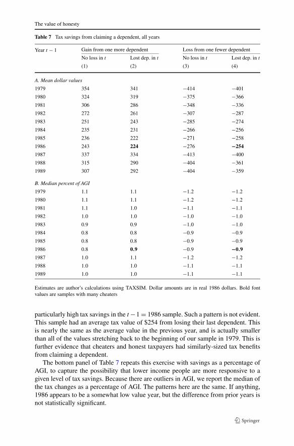
The value of honesty
Table 7 Tax savings from claiming a dependent, all years
Year t − 1 Gain from one more dependent Loss from one fewer dependent
No loss in t Lost dep. in t No loss in t Lost dep. in t
(1) (2) (3) (4)
A. Mean dollar values
1979 354 341 −414 −401
1980 324 319 −375 −366
1981 306 286 −348 −336
1982 272 261 −307 −287
1983 251 243 −285 −274
1984 235 231 −266 −256
1985 236 222 −271 −258
1986 243 224 −276 −254
1987 337 334 −413 −400
1988 315 290 −404 −361
1989 307 292 −404 −359
B. Median percent of AGI
1979 1.1 1.1 −1.2 −1.2
1980 1.1 1.1 −1.2 −1.2
1981 1.1 1.0 −1.1 −1.1
1982 1.0 1.0 −1.0 −1.0
1983 0.9 0.9 −1.0 −1.0
1984 0.8 0.8 −0.9 −0.9
1985 0.8 0.8 −0.9 −0.9
1986 0.8 0.9 −0.9 −0.9
1987 1.0 1.1 −1.2 −1.2
1988 1.0 1.0 −1.1 −1.1
1989 1.0 1.0 −1.1 −1.1
Estimates are author’s calculations using TAXSIM. Dollar amounts are in real 1986 dollars. Bold fontvalues are samples with many cheaters
particularly high tax savings in the t −1 = 1986 sample. Such a pattern is not evident.This sample had an average tax value of $254 from losing their last dependent. Thisis nearly the same as the average value in the previous year, and is actually smallerthan all of the values stretching back to the beginning of our sample in 1979. This isfurther evidence that cheaters and honest taxpayers had similarly-sized tax benefitsfrom claiming a dependent.
The bottom panel of Table 7 repeats this exercise with savings as a percentage ofAGI, to capture the possibility that lower income people are more responsive to agiven level of tax savings. Because there are outliers in AGI, we report the median ofthe tax changes as a percentage of AGI. The patterns here are the same. If anything,1986 appears to be a somewhat low value year, but the difference from prior years isnot statistically significant.

S. LaLumia, J.M. Sallee
Fig. 7 Distribution of tax values. Figure shows empirical distributions of the tax savings associated witha marginal dependent for those losing a dependent and those not losing a dependent in the policy changeyear (a) and earlier years (b). Panels (c) and (d) show the same statistics for the subset of filers that have anonzero tax value. All calculations are for tax values in year t − 1, where t is the year when the dependentwas lost
Figure 7 goes beyond comparisons of means by plotting the empirical cumulativedistribution of tax values for relevant subsamples. Figure 7a shows the distributionfor those who lost a dependent in 1987 and those who did not lose a dependent in1987. If the driving force behind cheating is tax savings, we would expect that thosewho lost a dependent in 1987—many of whom were cheaters—would have higher taxvalues than those who did not cheat. This is not the case. The distribution for thoselosing a dependent lies above the distribution for those who did not lose a dependent,which implies that they had lower gains from claiming an additional dependent.
Figure 7b shows the same comparison for years before the policy reform. The dis-tributions are fairly similar, though there is a difference in the number with a zero taxvalue—more of those who lost a dependent in pre-1987 years had a zero value froman additional dependent. To eliminate any differences in the distribution due strictlyto the zero values, Figs. 7c and 7d show the same distributions, limited to those withpositive estimated tax values. Now, the prereform years look very similar, which sug-gests that when there is no change in the incentive to cheat, the tax value distributionsof those losing a dependent and those not losing are quite similar. Nevertheless, the

The value of honesty
policy reform year still shows a difference—those who lost a dependent had lowertax values.
Overall, this evidence suggests that cheaters did not have especially large gainsfrom claiming additional children. This implies that the main driver of the decision tocheat was not the amount of money at stake. Since risk aversion plays a minor role inmodifying valuations, it is implausible that risk aversion heterogeneity is a dominantdriver, but we cannot rule out that heterogeneity in the perceived probability of auditand detection is key. It seems that either variation in the taste for honesty or variationin the perception of audit probabilities must be large.
7 Conclusion
The case of the missing children provides a unique opportunity for examining taxpay-ers’ evasion behavior. Two main lessons emerge from our analysis. First, this episodedemonstrates that while a substantial number of taxpayers lied to the IRS in order tosave on their taxes, a much larger fraction of taxpayers passed up an easily accom-plished evasion opportunity. These honest taxpayers gave up hundreds of dollars oftax savings, which amounted to an average of 7 % of their tax bill. This choice revealsa substantial and widespread willingness to pay to be honest. We think this is an im-portant addendum to recent research that concludes that evasion is driven primarilyby access to evasion opportunities and monitoring efficacy, as in Kleven et al. (2011).The evidence here suggests a greater role for a preference for honesty.
Second, the available evidence indicates that heterogeneity in willingness to cheatoutweighed heterogeneity in the tax savings associated with children in determin-ing who cheated and who did not. Cheaters do appear to be different from honesttaxpayers in some key characteristics, like filing status, but these differences do nottranslate to substantial differences in the average tax savings from claiming children.This suggests that something other than variation in the tax benefit of a child playsan important role in determining who cheated and who did not. We interpret this asevidence that there is important variation in the willingness to pay to be honest.
Finally, we believe that our methodology for inferring the characteristics ofcheaters, our use of a natural experiment, and our analysis of an evasion opportu-nity available to virtually all taxpayers constitute contributions to the larger literatureon the economics of income tax evasion. In particular, our work contributes to theemerging stream of research that studies “traces of evasion” (Slemrod and Weber2012) by showing an additional way of learning about evasion in the absence of auditdata.
Acknowledgements The authors would like to thank Jon Bakija, Brian Erard, Naomi Feldman, BillGentry, Jens Ludwig, Damon Jones, Lucie Schmidt, Joel Slemrod and seminar participants at the NationalTax Association and Universidad de Chile for helpful comments.
References
Allingham, M. G., & Sandmo, A. (1972). Income tax evasion: a theoretical analysis. Journal of PublicEconomics, 1, 323–338.

S. LaLumia, J.M. Sallee
Alm, J., McClelland, G. H., & Schulze, W. D. (1992). Why do people pay taxes? Journal of Public Eco-nomics, 48, 21–38.
Andreoni, J., Erard, B., & Feinstein, J. (1998). Tax compliance. Journal of Economic Literature, 36(2),818–860.
Attanasio, O. P., & Paiella, M. (2011). Intertemporal consumption choices, transaction costs and limitedparticipation in financial markets: reconciling data and theory. Journal of Applied Econometrics,26(2), 322–343.
Auten, G., & Carroll, R. (1999). The effect of income taxes on household income. Review of Economicsand Statistics, 81(4), 681–693.
Baldry, J. (1987). Income tax evasion and the tax schedule: some experimental results. Public Finance,42(3), 357–383.
Becker, G. S. (1968). Crime and punishment: an economic approach. Journal of Political Economy, 76(2),169–217.
Becker, W., Büchner, H.-J., & Sleeking, S. (1987). The impact of public transfer expenditures on taxevasion. Journal of Public Economics, 34, 243–252.
Block, M. K., & Heineke, J. M. (1975). A labor theoretic analysis of the criminal choice. American Eco-nomic Review, 65(3), 314–325.
Bordignon, M. (1993). A fairness approach to income tax evasion. Journal of Public Economics, 52, 345–362.
Chetty, R. (2006). A new method of estimating risk aversion. American Economic Review, 96(5), 1821–1834.
Christian, C. W. (1994). Voluntary compliance with the individual income tax: results form the 1988 TCMPstudy. In IRS research bulletin 1993/1994, publication 1500 (Rev. 9–94).
Christian, C. W., & Frischmann, P. J. (1989). Attrition in the statistics of income panel of individual returns.National Tax Journal, 42(4), 495–501.
Clotfelter, C. T. (1983). Tax evasion and tax rates: an analysis of individual returns. Review of Economicsand Statistics, 65(3), 363–373.
Cowell, F. A. (1992). Tax evasion and inequity. Journal of Economic Psychology, 13, 521–543.Crump, R., Goda, G. S., & Mumford, K. (2011). Fertility and the personal exemption: comment. American
Economic Review, 101(4), 1616–1628.DeLong, J. B., & Magin, K. (2009). The US equity return premium: past, present, and future. Journal of
Economic Perspectives, 23(1), 193–208.Dickert-Conlin, S., & Chandra, A. (1999). Taxes and the timing of births. Journal of Political Economy,
107(1), 161–177.Dubin, J. A., Graetz, M. J., & Wilde, L. (1990). The effect of audit rates on the federal individual income
tax, 1977–1986. National Tax Journal, 43(4), 395–409.Erard, B., & Feinstein, J. S. (1994). Honesty and evasion in the tax compliance game. Rand Journal of
Economics, 25(1), 1–19.Fack, G., & Landais, C. (2011). Charitable giving and tax policy in the presence of tax cheating: theory
and evidence from the US and France. Manuscript: Stanford University.Feenberg, D., & Coutts, E. (1993). An introduction to the TAXSIM model. Journal of Policy Analysis and
Management, 12(1), 189–194.Feinstein, J. S. (1991). An econometric analysis of income tax evasion and its detection. Rand Journal of
Economics, 22(1), 233–276.Feldman, N. E., & Slemrod, J. (2007). Estimating tax noncompliance with evidence from unaudited tax
returns. Economic Journal, 117, 327–352.Fisman, R., & Wei, S.-J. (2004). Tax rates and tax evasion: evidence from “missing imports” in China.
Journal of Political Economy, 112(2), 843–877.General Accounting Office (1993). Erroneous dependent and filing status claims. GAO/GGD-93-60.General Accounting Office (1996). Audit trends and results for individual taxpayers. GAO/GGD-96-61.Gordon, J. P. F. (1989). Individual morality and reputation costs as deterrents to tax evasion. European
Economic Review, 33, 797–805.Gruber, J. (2009). Public finance and public policy (3rd ed.). New York: Worth.Holtzblatt, J., & McCubbin, J. (2003). Whose child is it anyway? Simplifying the definition of a child.
National Tax Journal, 56(3), 701–718.Internal Revenue Service Oversight Board (2011). 2010 taxpayer attitude survey. US Department of the
Treasury January 2011.Jacob, B. A., & Levitt, S. D. (2003). Rotten apples: an investigation of the prevalence and predictors of
teacher cheating. Quarterly Journal of Economics, 118(3), 843–877.
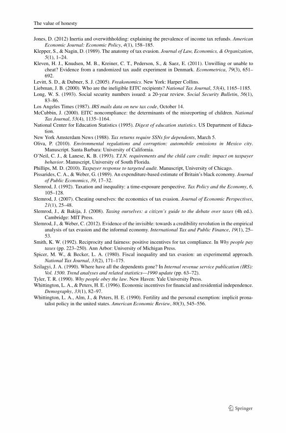
The value of honesty
Jones, D. (2012) Inertia and overwithholding: explaining the prevalence of income tax refunds. AmericanEconomic Journal: Economic Policy, 4(1), 158–185.
Klepper, S., & Nagin, D. (1989). The anatomy of tax evasion. Journal of Law, Economics, & Organization,5(1), 1–24.
Kleven, H. J., Knudsen, M. B., Kreiner, C. T., Pederson, S., & Saez, E. (2011). Unwilling or unable tocheat? Evidence from a randomized tax audit experiment in Denmark. Econometrica, 79(3), 651–692.
Levitt, S. D., & Dubner, S. J. (2005). Freakonomics. New York: Harper Collins.Liebman, J. B. (2000). Who are the ineligible EITC recipients? National Tax Journal, 53(4), 1165–1185.Long, W. S. (1993). Social security numbers issued: a 20-year review. Social Security Bulletin, 56(1),
83–86.Los Angeles Times (1987). IRS mails data on new tax code, October 14.McCubbin, J. (2000). EITC noncompliance: the determinants of the misreporting of children. National
Tax Journal, 53(4), 1135–1164.National Center for Education Statistics (1995). Digest of education statistics. US Department of Educa-
tion.New York Amsterdam News (1988). Tax returns require SSNs for dependents, March 5.Oliva, P. (2010). Environmental regulations and corruption: automobile emissions in Mexico city.
Manuscript. Santa Barbara: University of California.O’Neil, C. J., & Lanese, K. B. (1993). T.I.N. requirements and the child care credit: impact on taxpayer
behavior. Manuscript, University of South Florida.Phillips, M. D. (2010). Taxpayer response to targeted audit. Manuscript, University of Chicago.Pissarides, C. A., & Weber, G. (1989). An expenditure-based estimate of Britain’s black economy. Journal
of Public Economics, 39, 17–32.Slemrod, J. (1992). Taxation and inequality: a time-exposure perspective. Tax Policy and the Economy, 6,
105–128.Slemrod, J. (2007). Cheating ourselves: the economics of tax evasion. Journal of Economic Perspectives,
21(1), 25–48.Slemrod, J., & Bakija, J. (2008). Taxing ourselves: a citizen’s guide to the debate over taxes (4h ed.).
Cambridge: MIT Press.Slemrod, J., & Weber, C. (2012). Evidence of the invisible: towards a credibility revolution in the empirical
analysis of tax evasion and the informal economy. International Tax and Public Finance, 19(1), 25–53.
Smith, K. W. (1992). Reciprocity and fairness: positive incentives for tax compliance. In Why people paytaxes (pp. 223–250). Ann Arbor: University of Michigan Press.
Spicer, M. W., & Becker, L. A. (1980). Fiscal inequality and tax evasion: an experimental approach.National Tax Journal, 33(2), 171–175.
Szilagyi, J. A. (1990). Where have all the dependents gone? In Internal revenue service publication (IRS):Vol. 1500. Trend analyses and related statistics—1990 update (pp. 63–72).
Tyler, T. R. (1990). Why people obey the law. New Haven: Yale University Press.Whittington, L. A., & Peters, H. E. (1996). Economic incentives for financial and residential independence.
Demography, 33(1), 82–97.Whittington, L. A., Alm, J., & Peters, H. E. (1990). Fertility and the personal exemption: implicit prona-
talist policy in the united states. American Economic Review, 80(3), 545–556.