the valuation of cash flow forecasts: an empirical...
TRANSCRIPT

The Valuation of Cash Flow Forecasts: An Empirical Analysis
Steven N. Kaplan; Richard S. Ruback
The Journal of Finance, Vol. 50, No. 4. (Sep., 1995), pp. 1059-1093.
Stable URL:
http://links.jstor.org/sici?sici=0022-1082%28199509%2950%3A4%3C1059%3ATVOCFF%3E2.0.CO%3B2-Z
The Journal of Finance is currently published by American Finance Association.
Your use of the JSTOR archive indicates your acceptance of JSTOR's Terms and Conditions of Use, available athttp://www.jstor.org/about/terms.html. JSTOR's Terms and Conditions of Use provides, in part, that unless you have obtainedprior permission, you may not download an entire issue of a journal or multiple copies of articles, and you may use content inthe JSTOR archive only for your personal, non-commercial use.
Please contact the publisher regarding any further use of this work. Publisher contact information may be obtained athttp://www.jstor.org/journals/afina.html.
Each copy of any part of a JSTOR transmission must contain the same copyright notice that appears on the screen or printedpage of such transmission.
The JSTOR Archive is a trusted digital repository providing for long-term preservation and access to leading academicjournals and scholarly literature from around the world. The Archive is supported by libraries, scholarly societies, publishers,and foundations. It is an initiative of JSTOR, a not-for-profit organization with a mission to help the scholarly community takeadvantage of advances in technology. For more information regarding JSTOR, please contact [email protected].
http://www.jstor.orgSun Oct 21 09:39:23 2007

T H E JOURNAL OF FINANCE .VOL L, NO 4 . S E P T E M B E R 1995
The Valuation of Cash Flow Forecasts: An Empirical Analysis
STEVEN N. KAPLAN and RICHARD S. RUBACK
ABSTRACT
This article compares the market value of highly leveraged transactions (HLTs) to the discounted value of their corresponding cash flow forecasts. For our sample of 51 HLTs completed between 1983 and 1989, the valuations of discounted cash flow forecasts are within 10 percent, on average, of the market values of the completed transactions. Our valuations perform at least as well as valuation methods using comparable companies and transactions. We also invert our analysis by estimating the risk premia implied by transaction values and forecast cash flows, and relating those risk premia to firm and industry betas, firm size, and firm book-to-market ratios.
THISARTICLE COMPARES THE market value of management buyouts and leveraged recapitalizations to the discounted value of their corresponding cash flow forecasts. Most economists readily accept the concept of estimating market values by calculating the discounted value of the relevant cash flows. However, little empirical evidence exists that shows that discounted cash flows provide a reliable estimate of market value. This study provides evidence of a strong relation between the market value of the highly leveraged transactions (HLTs) in our sample and the discounted value of their corresponding cash flow forecasts.
Our tests compare the transaction values in HLTs to estimates of the present value of the relevant cash flows. We use a sample of management buyouts and leveraged recapitalizations because these transactions typically release the cash flow information and transaction value required for the analysis. We use the cash flow forecasts to estimate the cash flows that will accrue to all capital providers, including different classes of debt and equity.
* Graduate School of Business, University of Chicago and National Bureau of Economic Re- search (NBER), and Harvard Business School and NBER, respectively. Lori Kaufnlan, Betsy McNair, and Kelly Welch provided able research assistance. Yacine Ait-Sahalia, Willard Carleton, Eugene Fama, Wayne Ferson, Anthony Lynch, Thomas Lys, Wayne Mikkelson, Mark Mitchell, Kevin M. Murphy, Daniel Nelson, Mitch Petersen, Nick Polson, Art Raviv, Jay Ritter, Joe Rizzi, Rene Stulz (the editor), Theo Vermaelen, Robert Vishny, an anonymous referee, and seminar participants at Arizona, Harvard, Illinois, the NBER Summer Institute, North Carolina, North- western, Oregon, Vanderbilt, Washington, and the University of Chicago provided helpful com- ments. This research was supported by the William Ladany Faculty Research Fund, the Center For Research in Security Prices, the Lynde and Harry Bradley Foundation, the Olin Foundation (Kaplan), and the Division of Research at Harvard Business School (Ruback). Address correspon- dence to Steven Kaplan at Graduate School of Business, University of Chicago, 1101 East 58th St., Chicago, IL 60637.
1060 The Journal of Finance
We estimate a terminal value when the cash flow information ends. We value the capital cash flows and the terminal value using a discount rate based on the Capital Asset Pricing Model (CAPM). The resulting median estimates of discounted cash flows are within 10 percent of the HLT transaction values. Furthermore, the prediction errors of the discounted cash flow estimates (relative to transaction values) are qualitatively similar to those found in previous work for option pricing models (relative to call option prices).
We compare the performance of our discounted cash flow estimates to that of estimates obtained from alternative valuation approaches that rely on companies in similar industries and companies involved in similar transac- tions. Such alternative valuation approaches-known as comparable or mul- tiple approaches-are commonly used in practice. The discounted cash flow (DCF) methods, individually, perform at least as well as the comparable methods. However, we also find the comparable approaches to be useful, especially when combined with a discounted cash flow valuation.
The discounted cash flow methods we use generally parallel the basic tech- niques taught in most business schools. Our results suggest that those tech- niques are both useful and reliable. We stress that our valuations rely on several ad hoc assumptions that readers (both academics and practitioners) should be able to improve on in a specific valuation. Furthermore, the dis- counted cash flow valuations succeed despite the additional concerns posed by HLTs beyond those associated with capital market imperfections and inter- temporal asset pricing models in any valuation problem. First, the cash flow forecasts come from published legal filings and may not be constructed to be estimates of expected cash flows. Second, even if the cash flow forecasts are intended to be expected cash flows, the forecasting process is likely to involve substantial errors because major organizational changes often accompany the HLTs. Finally, since these firms have extremely leveraged capital structures, their access to capital markets and their ability to use interest tax shields may be limited. Greater attention to individual assumptions and to the HLT com- plications would presumably lead to better DCF valuations.
We also invert our analysis to calculate an implied discount rate-the discount rate that equates the discounted cash flow forecasts to the transaction value. The median implied market equity risk premium (7.78 percent) we obtain from this calculation is comparable to the historic arithmetic average market equity risk premium. We also examine the relation of the implied risk premia to firm size, firm book-to-market ratios, and systematic risk measures to determine if our results are consistent with Fama and French (1992), who find that firm equity returns are related to firm equity values and book-to- market ratios, but not to measures of systematic risk. We find that the implied risk premia are not significantly related to firm size or pretransaction book- to-market ratios, but are positively related to firm and industry betas. For this sample, therefore, we favor CAPM-based approaches to discount rates over those based on size or book-to-market ratios.

The Valuation of Cash Flow Forecasts: A n Empirical Analysis 1061
The success of the discounted cash flow valuation approaches in spite of the leveraged capital structures and overall complexity of the HLTs raises con- cerns that there is something special about our sample of HLTs. The primary concern is that the cash flows might somehow be endogenous, and that endo- geneity causes the DCF valuations to be spurious estimates of transaction value. One potential source of endogeneity is that dealmakers and managers in the HLTs may have had incentives to adjust the cash flow forecasts. For example, incentives to bias the cash flow forecasts upward are present when the true expected cash flows are below the level required to obtain transaction financing. Alternatively, incentives to bias the forecasts downward are present when the true expected cash flows are substantially above those needed to obtain financing. Because the SEC and courts effectively require the board of directors of the HLT company to obtain an opinion from an investment bank that the transaction price is "fair," insiders and dealmakers may have an incentive to reduce their reported cash flow forecasts to justify the transaction price.
We conduct several tests to detect the presence of such adjustments. We examine the ex post accuracy of the cash flow forecasts and find only modest evidence of ex ante bias. We divide our sample into subsamples based on leverage and outside competition, and find little difference across the sub- samples. Finally, we use our discounted cash flow valuation technique to value initial public offerings where the leverage and incentives to adjust cash flow forecasts are different from those in our HLT sample. We find that our valuations provide reliable estimates of value for the sample of initial public offerings. Overall, we find little evidence to suggest that the reliability of our discounted cash flow approaches is restricted to HLTs.
The article proceeds as follows. Section I explains our basic valuation ap- proach in more detail. Section I1describes the data set along with some sample statistics. Section I11 presents the valuation results and compares those re- sults to transaction values. Section IV calculates implied risk premia and compares them to firm betas, industry betas, firm size, and firm book-to- market ratios. Section V discusses and addresses potential criticisms of our results based on the incentives to adjust cash flow forecasts. Section VI summarizes the results and presents our conclusions.
I. Valuation Techniques
A. Transaction Value
In our analyses, we compare estimates of value to the portion of actual market value that reflects future cash flows. We define the transaction value as the market value of the firm's future cash flows. The total market value of the firm equals the value of a firm's future cash flows and the firm's current excess cash. We subtract excess cash, measured as cash balances and marketable securities, from total market value to obtain our estimate of the transaction value of the firm's future cash flows. We obtain similar results when we

1062 The Journal o f Finance
s.ubtract, instead, only the excess cash used to finance the transaction. Our measure of transaction value, therefore, assumes that long-term assets and net working capital (excluding excess cash) are used to generate the cash flows of the firm. Specifically, we calculate transaction value as: 1)the market value of the firm's common stock; 2) plus the market value of the firm's preferred stock; plus 3) the value of the firm's debt; plus 4) transaction fees; less 5 ) the firm's cash balances and marketable securities. All of these are measured at the closing of the transaction. Debt that is not repaid as part of the transaction is valued at book value. Debt that is repaid is valued at the repayment value.
B. The Compressed Adjusted Present Value Technique
The Compressed Adjusted Present Value Technique (Compressed APV) that we use values firms by discounting capital cash flows at the discount rate for an all-equity firm.1 Capital cash flows equal the after-corporate-tax cash flows to both debt and equity holders of the firm. Because the cash flows are measured after corporate tax, the tax benefits of deductible interest payments are included in the cash flows. The interest tax shields reduce income taxes and, thereby, raise after-corporate-tax cash flows. Our use of the Compressed APV method is equivalent to using the adjusted present value (APV) method and discounting interest tax shields at the discount rate for an all-equity firm. This assumes that the interest tax shields have the same systematic risk as the firm's underlying cash flows. An alternative way to interpret the Com- pressed APV method is that of discounting the capital cash flows at the before-tax discount rate that is appropriate for the riskiness of the cash flows.
The Compressed APV method simplifies the valuation of HLTs. The widely used after-tax weighted average cost of capital (WACC) approach is apprecia- bly more difficult to implement. The WACC approach requires that the cost of capital be recomputed each period to include the effect of changing leverage over time. It also requires additional assumptions about the firm's tax status to generate cash flows assuming an all-equity ~apitalization.~ The Compressed APV also has a computational advantage over the standard APV approach, because the standard APV approach requires that the all-equity cash flows and the interest tax shields be discounted separately at different discount rates.
B.1. Measuring Capital Cash Flows
We measure capital cash flows in two ways, depending on the presentation of the cash flow forecasts for the HLTs in our sample. The first method begins with net income. We add adjustments for the differences between accounting information and cash flows. These adjustments include depreciation, amorti- zation, changes in net working capital, and interest. We also add changes in
We would like to thank Stewart Myers for suggesting "Compressed APV" as a label for this method.
See Ruback (1989 and 1994) for additional background on the Compressed APV technique and its relation to the weighted average cost of capital approach.
-- --
The Valuation of Cash Flow Forecasts: A n Empirical Analysis 1063
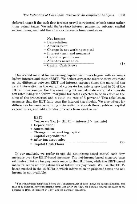
deferred taxes if the cash flow forecast provides reported or book taxes rather than actual taxes. We add (before-tax) interest payments, subtract capital expenditures, and add the after-tax proceeds from asset sales.
Net Income + Depreciation + Amortization - Change in net working capital + Interest (cash and noncash) - Capital expenditures + After-tax asset sales = Capital Cash Flows
Our second method for measuring capital cash flows begins with earnings before interest and taxes (EBIT). We deduct corporate taxes that we estimate as the difference between EBIT and interest expense times the marginal tax rate. Information on the marginal corporate tax rate is provided in 33 of the HLTs in our sample. For the remaining 18, we calculate marginal corporate tax rates using the federal marginal tax rates expected to be in effect at the time of the transaction and a state tax rate of 5 percenL3 This calculation assumes that the HLT fully uses the interest tax shields. We also adjust for differences between accounting information and cash flows, subtract capital expenditures, and add after-tax proceeds from asset sales:
EBIT - Corporate Tax [= (EBIT - interest) X tax rate] + Depreciation+ Amortization - Change in net working capital - Capital expenditures + After-tax asset sales = Capital Cash Flows (2)
In our analysis, we prefer to use the net-income-based capital cash flow measure over the EBIT-based measure. The net-income-based measure uses estimates of future tax payments made by the HLT firm, while the EBIT-based measure relies on our estimates of future tax payments. We use the EBIT- based method in the 15 HLTs in which information on projected taxes and net income is not available.
For transactions completed before the Tax Reform Act of 1986 (TRA),we assume a federal tax rate of 46 percent. For transactions completed after the TRA, we assume federal tax rates of 46 percent in 1986, 38 percent in 1987, and 34 percent thereafter.

1064 The Journal of Finance
B.2. Terminal Values
We obtain terminal values by calculating a terminal capital cash flow and assuming that terminal capital cash flow will grow at a constant nominal rate in perpetuity.
The calculation of the terminal capital cash flow begins with the capital cash flow in the last forecast year and adjusts for the difference between capital expenditures and depreciatioh and amortization. Assuming a growing perpe- tuity, capital expenditures should be at least as large as depreciation and amortization. On average, however, depreciation and amortization exceed capital expenditures in the last forecast year for our sample of HLTs. In practice, armed with more information about depreciation schedules, it would be possible to adjust for this inconsistency by forecasting steady-state depre- ciation. In our analysis, we (partially) eliminate the inconsistency by setting depreciation and amortization equal to capital expenditures in the capital cash flow in the last forecast year. We call this adjusted cash flow the terminal capital cash fl0w.4
The growth in the nominal terminal capital cash flow should reflect both expected inflation growth and real growth. Unfortunately, only 11of 51 sample transactions explicitly note an expected inflation rate. The average expected inflation rate is 5 percent. Actual inflation (as measured by growth of the GNP deflator) averaged 3.4 percent per year between 1983 and 1989. In 1988, the year almost 50 percent of our transactions were priced, the GNP deflator increased by 3.3 percent. We present our results using a nominal growth rate of 4 percent, which corresponds to a real growth rate between 0 percent and 1 percent. We also report the sensitivity of our results to different terminal cash flow growth rates.
B.3. Discount Rates
We discount the capital cash flows using the expected return implied by the Capital Asset Pricing Model for the unlevered firm:
where r fis the risk free rate, puis the firm's unlevered beta or systematic risk, and r , - r f is the risk premium required by investors to invest in a firm or project with the same level of systematic risk as the stock market.
We use the unlevered (or all-equity) cost of capital because it is a reasonable estimate of the riskiness of the firm's assets. Our cash flow measure includes all of the cash flows generated by the assets, including interest tax shields. Under the assumption that the riskiness of these cash flows is the same as that of the firm's assets, the unlevered cost of capital is the appropriate discount rate using the Capital Asset Pricing Model. This method is equivalent to using
We obtain qualitatively similar results when we repeat the analyses with no adjustment, and with capital expenditures set equal to depreciation and amortization.

The Valuation of Cash Flow Forecasts: A n Empirical Analysis 1065
the Adjusted Present Value method (see Brealey and Myers (1991)) and dis- counting the forecast interest tax shields at the unlevered cost of capital.5
The unlevered cost of capital also can be interpreted as the before-corporate- tax, weighted average cost of capital. The before-tax discount rate is appropri- ate to discount capital cash flows because the tax benefits of interest are included in our cash flow measure. By adjusting the cash flows for taxes and applying Modigliani and Miller (1963), the weighted average cost of capital is the same for different levels of leverage and we do not have to estimate the cost of debt.
We present valuations using three different measures of systematic risk. First, we use a firm-based measure. We estimate equity P's, Pe, using daily stock returns, returns on the S&P 500, and a Dimson (1979) correction. Returns are used from 540 to 60 days before the transaction is announced. To obtain flu, we unlever Pe:
where E equals the market value of firm equity 60 days before the transactions is announced, P equals the (book) liquidation value of non-convertible pre- ferred stock, and D equals net debt-the book value of short-term and long- term debt, less cash and marketable securities at the time of the transaction. We assume the systematic risk of the preferred stock and the debt, PP and pd, with respect to returns on the S&P 500 equal 0.25-the beta reported for high grade debt from 1977 to 1989 in Cornell and Green (1991).6 Finally, the tax rate, r, equals the combined marginal federal and state tax rate during the estimation period. Consistent with the low pre-HLT debt levels of the sample firms, this pU calculation assumes that the pre-HLT tax shield has the same risk characteristics as pre-HLT debt.
Second, we use an industry-based measure of systematic risk. We calculate industry equity betas using daily returns from a value-weighted portfolio of all New York and American Stock Exchange companies in the same two-digit SIC code as the sample companies. The industry equity betas are calculated from 540 to 60 days before the transaction is announced using returns on the S&P 500, and a Dimson (1979) correction. We use equation (4) to unlever the industry equity betas with the value-weighted ratios of equity, preferred, and debt to total capital for firms in the relevant industry. These industry ratios
This analysis values interest tax shields a t the full corporate tax rate, but assumes that the ability to use the tax shields has the same systematic risk as the (cash flows of the) unlevered or all-equity firm. These simplifying assumptions have two offsetting effects on our estimated values. First, the expected values of the interest tax shields in reality are less than those implied by the corporate tax rate because there is a nontrivial probability that a given HLT firm will suffer losses and be forced to carry forward some interest tax shields. Accounting for this would lower our estimated values. On the other hand, the ability to use the interest tax shields has less systematic risk than the unlevered firm because the expected value of the tax shields does not increase once the firm is fully taxable. Accounting for this would raise our estimated values.
Only 7 of the sample companies have any such preferred outstanding.

1066 The Journal of Finance
are calculated using COMPUSTAT data for the fiscal year ending before the HLT is announced.
Third, we use a market-based measure of systematic risk that assumes that the systematic risk for all sample firms equals the risk of the assets of the market. To obtain the market asset beta, we calculate the leverage of nonfi- nancial and nonutility firms in the S&P 500. The median leverage ratio during the sample period, 1983 to 1989, was 0.20. Combining the market leverage in the year before the transaction, a debt beta of 0.25, and adjusting for taxes using equation (4), the median unlevered asset beta for the market equals 0.91.
We calculate the risk premium as the arithmetic average return spread between the S&P500 and long-term Treasury bonds from 1926 until the year before the transaction is announced. For our sample firms, the median risk premium is 7.42 percent. In using this risk premium, we are following the general recommendation in finance texts to use the arithmetic average histor- ical risk premium. (For example, see Brealey and Myers (1991)). The historical arithmetic average risk premium approach implicitly assumes 1)that returns are independent; and 2) that the underlying probability distribution is stable. There is some disagreement about the appropriateness of the arithmetic av- erage measure of risk premia. Some are concerned that evidence of autocor- relation in returns suggests that returns are not independent. Others are concerned about the stability of the distribution; Blanchard (1993), for exam- ple, argues that the equity risk premium declined to 3 percent or 4 percent by the end of the 1980s. The reasonableness of our choice is an empirical question that we implicitly test in Section I11 and explicitly consider in Section IV.
Finally, we use the long-term (approximately 20 years to maturity) Treasury bond yield to measure the risk-free rate in our cost of capital calculations. Long-term Treasury bond yields, by month, are obtained from Ibbotson Asso- ciates (1991). Our specifications implicitly assume a long-term investment horizon. However, we obtain qualitatively similar results when we base our analyses on a short-term investment horizon. For a short-term horizon, we estimate the risk-free rate as the long-term Treasury bond yield less the historic arithmetic average spread between Treasury bond and Treasury bill returns, and we use a risk premium equal to the long-term arithmetic average return spread between the S&P 500 and Treasury bills.
C. Valuation Methods Using Comparables
Practitioners often value companies using trading or transaction multiples. In these methods, a ratio or multiple of value relative to a performance measure is calculated for a set of guideline or comparable firms. Earnings before interest, taxes, depreciation, and amortization (EBITDA) and earnings before interest and taxes (EBIT), net income, and revenue are commonly used performance measures. Value is estimated by multiplying the ratio or multiple from the guideline companies by the performance measure for the company being valued.

The Valuation of Cash Flow Forecasts: An Empirical Analysis 1067
Valuation by comparables or multiples relies on two assumptions. First, the comparable companies have future cash flow expectations proportional to and risks similar to those of the firm being valued. Second, the performance measure (like EBITDA) is actually proportional to value. If these assumptions are valid, the comparable method will provide a more accurate measure of value than any discounted cash flow approach because it incorporates contem- poraneous market expectations of future cash flows and discount rates in the multiple. In practice, however, the comparable companies are not perfect matches in the sense that cash flows are not proportional and risks are not similar. Also, there is no obvious method to determine which measure of performance-EBITDA, EBIT, net income, revenue, and so on-is the most appropriate for comparison. Consistent with these concerns, Kim and Ritter (1994) find that comparable methods are not particularly successful in pricing initial public offerings.
The discounted cash flow method relies on forecast cash flows that directly relate to the firm being valued and discount rates which are based on the historical riskiness of the firm or its industry. The reliability of the discounted cash flow valuation depends on the accuracy of the cash flow projections, risk measures, and the assumptions used in calculating the cost of capital, includ- ing the historical measure of the risk premium. Both the discounted cash flow methods and the comparable firm methods therefore have inherent estimation errors. The empirical issue is whether the benefits of using firm-specific information in the discounted cash flow method are greater than the costs of ignoring the contemporaneous measures of market expectations contained in the comparable methods.
To make the values estimated with multiples comparable to those estimated using capital cash flows, we base our multiples on EBITDA. We use three different measures of guideline or comparable companies. The first, which we label comparable company, uses a multiple calculated from the trading values of firms in the same industry as the firm being valued. The second, which we label comparable transaction, uses a multiple from companies that were in- volved in a similar transaction to the company being valued. The third, which we label comparable industry transaction, uses a multiple from companies in the same industry that were involved in a similar transaction to the company being valued.
We construct comparable company value as the sample firm's EBITDA in the year before the transaction multiplied by the median industry multiple of total capital value in the month of the transaction to EBITDA in the year before the transaction. Total capital value is the analog of transaction value, equalling the sum of the market value of common stock, the liquidation value of firm preferred stock, and the book value of firm short- and long-term debt, less the cash balances and marketable securities of the firm. To get as close a match as possible, we calculate the industry multiples using companies (on COMPUSTAT) with the same four-digit Standard Industrial Classification (SIC) code and with total capitalizations of at least $40 million. If there are

1068 The Journal of Finance
fewer than five comparable companies at the four-digit level, we match com- panies at the three-digit level, and, if necessary, at the two-digit level.
We calculate comparable transaction value as the sample firm's EBITDA in the year before the transaction times the median ratio of total transaction value to EBITDA (in the year before the transaction) for comparable HLTs. Comparable HLTs are those HLTs among the 136 in Kaplan and Stein (1990 and 1993) that are priced within one year of the date the sample transaction is priced.
Comparable industry transaction values combine the comparable company and comparable transaction approaches by estimating comparable transaction values for HLTs in the same industry. We use the sample firm's EBITDA in the year before the transaction times the median multiple of total transaction value to EBITDA in the year before the transaction for HLTs in the same 2-digit SIC code that are priced within two years of the date the sample transaction is priced. We are unable to obtain an acceptable comparable industry HLT for more than one-quarter of the HLTs (13 of 51), and, therefore, the sample size for this measure is lower. Because the sample from which we draw the comparables includes a large fraction of the HLT universe, we do not believe this is a sample-specific problem.
11. Data
Our sample of companies starts with two sources of highly leveraged trans- actions. First, we use the sample of 124 management buyouts (MBOs) ana- lyzed by Kaplan and Stein (1993). These buyouts satisfy four conditions: l)the companies are originally publicly owned; 2) the transaction is completed be- tween 1980 and 1989; 3) at least one member of the incumbent management team obtains an equity interest in the new private firm; and 4) the total transaction value exceeds $100 million.
We add to this the sample of 12 leveraged recapitalizations examined by Kaplan and Stein (1990). A leveraged recapitalization is similar to a MBO in many respects except that it does not involve the repurchase of all of a company's stock. While there is a dramatic increase in leverage, public stock- holders retain some interest in the company. These leveraged recapitalizations were completed between 1985 and 1989.
We examined the documents describing the transactions that these firms filed with the SEC. These documents include proxy statements, Schedule 14D tender offer filings, and Schedule 13E-3 filings. Rule 13E-3 applies to trans- actions in which insiders potentially stand to benefit at the expense of outside, public shareholders. Item 8 of Rule 13E-3 requires the HLT's board of directors to indicate whether the transaction is fair (or unfair) to public shareholders, and to provide a detailed discussion of the basis for that opinion. Item 9 further requires the HLT board to furnish a summary of any report from an outside party that relates to the opinion in Item 8. The disclosure in Item 9 usually includes cash flow forecasts. Accordingly, all but 12 of the 136 companies provide some post-transaction financial projections or forecasts.
The Valuation of Cash Flow Forecasts: A n Empirical Analysis 1069
Table I
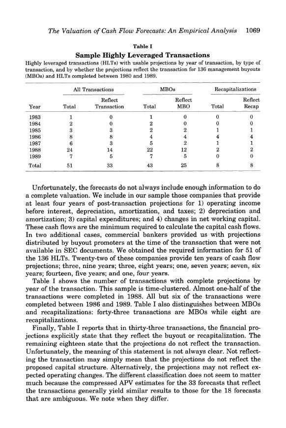
Sample Highly Leveraged Transactions Highly leveraged transactions (HLTs) with usable projections by year of transaction, by type of transaction, and by whether the projections reflect the transaction for 136 management buyouts (MBOs) and HLTs completed between 1980 and 1989.
All Transactions MBOs Recapitalizations
Year Total Reflect
Transaction TReflect
otal MBO Total Reflect Recap
1983 1984 1985 1986 1987 1988 1989
0 0 1 4 1 2 0
0 0 1 4 1 2 0
Total
Unfortunately, the forecasts do not always include enough information to do a complete valuation. We include in our sample those companies that provide at least four years of post-transaction projections for 1)operating income before interest, depreciation, amortization, and taxes; 2) depreciation and amortization; 3) capital expenditures; and 4) changes in net working capital. These cash flows are the minimum required to calculate the capital cash flows. In two additional cases, commercial bankers provided us with projections distributed by buyout promoters at the time of the transaction that were not available in SEC documents. We obtained the required information for 51 of the 136 HLTs. Twenty-two of these companies provide ten years of cash flow projections; three, nine years; three, eight years; one, seven years; seven, six years; fourteen, five years; and one, four years.
Table I shows the number of transactions with complete projections by year of the transaction. This sample is time-clustered. Almost one-half of the transactions were completed in 1988. All but six of the transactions were completed between 1986 and 1989. Table I also distinguishes between MBOs and recapitalizations: forty-three transactions are MBOs while eight are recapitalizations.
Finally, Table I reports that in thirty-three transactions, the financial pro- jections explicitly state that they reflect the buyout or recapitalization. The remaining eighteen state that the projections do not reflect the transaction. Unfortunately, the meaning of this statement is not always clear. Not reflect- ing the transaction may simply mean that the projections do not reflect the proposed capital structure. Alternatively, the projections may not reflect ex- pected operating changes. The different classification does not seem to matter much because the compressed APV estimates for the 33 forecasts that reflect the transactions generally yield similar results to those for the 18 forecasts that are ambiguous. We note when they differ.
1070 The Journal of Finance
For each transaction with complete projections, we obtain information de- scribing the transactions from proxy, 13E-3, or 14D statements. Stock prices two months before the transaction announcement and at transaction comple- tion are obtained from the Center for Research in Security Prices (CRSP) database and Standard & Poor's Daily Stock Price Record. Other financial data are obtained from the COMPUSTAT Tapes. For more details on these trans- actions, see Kaplan and Stein (1990 and 1993).
In Section V, we address possible endogeneity issues by performing similar analyses for cash flow forecasts of a smaller sample of eight initial public offerings (IPOs) completed between October 1991 and July 1992. The IPO firms are firms that had previously gone private in leveraged buyouts. Because the IPOs involved refinancing existing loans, the IPO firms provided cash flow forecasts to commercial bankers who held the loans, and we obtained the forecasts from those bankers. These cash flow forecasts are not available in SEC documents and, therefore, were not available to public shareholders.
111. Valuation Results
A. Compressed APV Methods
Panel A of Table I1 presents summary statistics for the valuation or estima- tion errors of the three discounted cash flow and three comparable valuation methods. The errors are computed as the log of the ratio of our estimated values to the transaction value. We use the log ratio because it is symmetric with respect to overestimates and underestimates. We present the errors in percent so that they can be interpreted as the percentage differences between the estimated value and the transaction value.
Focusing on the Compressed APV estimates using firm-specific betas, Panel A reports that the median error is 6.0 percent, which means that the DCF estimate is 6.0 percent greater than the transaction value. Across the Com- pressed APV measures, the median errors are 6.2 percent for the industry- based estimates, and 2.5 percent for the market-based estimates. The median errors for the market-based estimates are not significantly different from zero. The mean errors are similar with the estimates based on firm-based betas overestimating transaction values the most, industry-based beta estimates exhibiting less of an overestimate of value, and the market-based beta esti- mates being closest to transaction value. The variation in the valuation errors is also greatest for the firm-based beta estimates.
Panel B of Table I11 presents median estimation errors for different equity risk premia. The results indicate that recommendations to use lower risk premia would reduce the accuracy of the discounted cash flow estimates of value. For example, if we use a risk premium of 6 percent, the median errors increase to 16.4 percent for the firm-based beta estimates, to 17.7 percent for the industry-based estimates, and to 13.6 percent for the market-based estimates. In contrast, when a higher risk premium is used, such as 9 percent, the median errors of the firm-based, industry-based, and market-based er-

The Valuation of Cash Flow Forecasts: An Empirical Analysis 1071
Table I1
Comparison of Different Valuation Methods Comparison of Capital Asset Pricing Model (CAPM)-based and comparable-based valuation meth- ods in 51 highly leveraged transactions completed between 1983 and 1989. The first four rows present the medians, means, standard deviations, and interquartile ranges of the valuation errors. The valuation errors equal the natural log of estimated values relative to transaction values. Valuation errors are reported in percent. Performance measure 1is the percentage of transactions in which absolute value of the valuation errors is less than or equal to 15 percent. Performance measure 2 is the mean absolute error of the valuation errors (in percent). Performance measure 3 is the mean squared error of valuation errors (in percent). CAPM-based values are the estimated present values of projected capital cash flows. Terminal values are grown a t 4 percent. Discount rates equal the long-term Treasury bond yield at the time of the projections plus the equity risk premium times the relevant asset beta. The risk premium is the arithmetic average premium of the S&P 500 return over the long-term Treasury bond return from 1926 until the year before the transaction is announced. Estimated present values are calculated using (A) CAPM-based ap- proach with firm asset betas; (B) CAPM-based approach with industry asset betas from value- weighted industry portfolios; (C) CAPM-based approach with market asset betas. Comparable values are calculated using (D) comparable company approach; (E) comparable transaction ap- proach; and (F) comparable industry transaction approach (for which observations are limited to 38 transactions). The transaction value equals (1)market value of the firm common stock; plus (2) market value of firm preferred stock; plus (3)value of firm debt; plus (4) transaction fees; less (5) firm cash balances and marketable securities, all a t the time of the transaction. Debt not repaid in the transaction is valued at book value; debt that is repaid, a t the repayment value.
CAPM-Based Valuation Methods Comparable Valuation Methods
(F) Comparable
(A) (B) (C) (D) (E Industry Firm Industry Market Comparable Comparable Transaction Beta Beta Beta Company Transaction (N= 38)
Panel A: Summary Statistics for Valuation Errors
1. Median 6.0% 6.2% 2.5% -18.1% 5.9% -0.1% 2. Mean 8.0% 7.1% 3.1% -16.6% 0.3% -0.7% 3. Standard deviation 28.1% 25.1% 22.6% 25.4% 22.3% 28.7% 4. Interquartile range 31.3% 23.0% 27.3% 41.9% 32.2% 23.7% 5. Asset beta (median) 0.81 0.84 0.91
Panel B: Performance Measures for Valuation Errors
1. Percentage within 15% 47.1% 62.7% 58.8% 37.3% 47.1% 57.9% 2. Mean absolute error 21.1% 18.1% 16.7% 24.7% 18.1% 20.5% 3. Mean squared error 8.4% 6.7% 5.1% 9.1% 4.9% 8.0%

1072 The Journal of Finance
Table I11
Sensitivity of CAPM-Based Approaches to Equity Risk Premium, Terminal Value Growth Rate, and Reflecting Transaction
Sensitivity of Capital Asset Pricing Model (CAPMI-based valuation methods to equity risk pre- mium, terminal value growth rate assumptions, and whether the projections explicitly reflect the transaction in 51 highly leveraged transactions (HLTs) completed between 1983 and 1989. Median is the median of the valuation errors (in percent). The valuation errors equal the natural log of estimated values relative to transaction values. Mean absolute error is the mean absolute error of the valuation errors. CAPM-based values are the estimated present values of projected capital cash flows. Discount rates equal the long-term Treasury bond yield a t the time of the projections plus the equity risk premium times the relevant asset beta. In the base case in Panel A, terminal values are grown a t 4 percent and the equity risk premium is the arithmetic average premium of the S&P 500 return over the long-term Treasury bond return from 1926 until the year before the transaction is announced. The median risk premium in the base case is 7.42 percent. In Panel B, values are estimated using equity risk premiums of 5, 6, and 9 percent. In Panel C, values are estimated using terminal value growth rates of 0,2,6, and 8 percent. Estimated present values are calculated using (A) CAPM-based approach with firm asset betas; (B) CAPM-based approach with industry asset betas from value-weighted industry portfolios; (C) CAPM-based approach with market asset betas. Transaction value equals (1)market value of the firm common stock; plus (2) market value of firm preferred stock; plus (3)value of firm debt; plus (4) transaction fees; less (5) firm cash balances and marketable securities, all a t the time of the transaction. Debt not repaid in the transaction is valued a t book value; debt that is repaid, a t the repayment value.
Valuation Errors for CAPM-Based Valuation Methods
Terminal Equity Median Mean Absolute Error
Value Risk (A) (B) (C) (A) (B) (C) Growth Premium Firm Industry Market Firm Industry Market
Rate (Median) Beta Beta Beta Beta Beta Beta
Panel A: Base Case
4% 7.42% 6.0% 6.2% 2.5% 21.1% 18.1% 16.7%
Panel B: Vary Equity Premium
Panel C: Vary Terminal Value Growth Rate
Panel D: 33 HLTs in Which Projections Explicitly Reflect Transactions

The Valuation of Cash Flow Forecasts: A n Empirical Analysis 1073
rors decline, with errors of -2.3 percent, -3.1 percent, and -7.6 percent, respectively.
We also experimented with beta estimation techniques that adjust for the tendency of betas to regress to the mean in future periods.7 These adjustments included using 1)equity betas that equal an equal-weighted average of the firm or industry beta and the market beta, i.e., estimates that push the firm or industry equity betas toward one; 2) the Bayesian approach in Vasicek (1973) that estimates equity betas as a weighted average of firm equity betas and the sample mean using the historical distribution of the sample beta coefficients; and 3) the Bayesian approach in Stevens (1993) that estimates equity betas using information in firm and industry equity betas. These methods are basically weighted averages of those presented in Table 11, and the results using these different techniques are roughly combinations of those reported in Table 11.
Panel C of Table I11 reports median estimation errors for different assump- tions about terminal value growth. Values increase as the terminal value growth rate increases. At no growth, median errors for the Compressed APV methods vary from -7.0 percent to -10.7 percent. At 2 percent growth, the Compressed APV methods are close to zero, especially for the firm-based beta estimates. For growth rates above 4 percent, the median errors for all of the Compressed APV methods are substantially greater than zero. Overall, these results suggest that our selection of 4 percent for the growth rate for terminal cash flows is reasonable.
The ordering of the accuracy of the Compressed APV measures based on medians depends on the assumptions and the sample selection. Panels B and C of Table I11 indicate that assumptions about risk premia and growth rates shift the distribution of value estimates. And Panel D of Table I11 shows that the median errors for the industry-based and market-based beta estimates both rise relative to the firm-based beta estimates for the subsample of 33 observations that explicitly reflect the transactions. The results for the medi- ans, therefore, suggest that the Compressed APV methods are reliable and useful measures of value, but do not provide enough basis to discriminate among the Compressed APV methods.
B. Comparable Methods
Panel A of Table I1 also reports the valuation errors when value is estimated using the three comparable methods. The estimates based on the comparable company method substantially underestimate transaction value, with a me- dian estimation error of -18.1 percent. This is well outside the range of median errors for the Compressed APV methods.
The comparable transaction based estimates are more accurate, with a median error of 5.9 percent, which is in the range of median errors for the Compressed APV estimates. In fact, the mean valuation error of 0.3 percent for
See Blume (1975) and Klemkosky and Martin (1975).

1074 The Journal of Finance
the comparable transactions is closer to zero than the mean valuation errors for the Compressed APV estimates.
The most accurate estimates are those for the comparable industry trans- action method with median and mean valuation errors of -0.1 percent and -0.7 percent. This method has the highest standard deviation, however, suggesting that the accuracy varies across firms in the sample. This highlights the fact that the method is not generally applicable because it is difficult to match both the industry and the transaction. We were unable to find matches for 13 of the 51 firms in our sample during a period in which there were a relatively large number of HLTs. In other samples and time periods, we suspect this problem would be even worse. This method also is difficult to generalize to other common valuation problems, such as capital investment decisions, because there is typically no transaction to match.
We also examined (but do not report in the tables) hybrid approaches in which we estimate the terminal value as the product of the (current) compa- rable company EBITDA multiple and the EBITDA forecast in the last year of the projections. These approaches are commonly used by investment bankers. We then discount the capital cash flows and terminal value at the discount rate for one of the three APV approaches. We performed this analysis using all years of projected cash flows as well as using only two, three, or four years of projected cash flows. In the median HLT for all of these approaches, the estimated values exceed transaction values by more than 10 percent. For example, using a market-based discount rate and all years of projections, we find that the median estimated value exceeds the transaction value by 18.7 percent.
The likely explanation for the poor performance of the hybrid approaches is that the EBITDA multiple at the time of the transaction includes a weighted average of higher growth during the forecast period and lower growth after the forecast period. By using the cash flows forecast over the forecast period and then applying the current EBITDA multiple at the end of the period, the
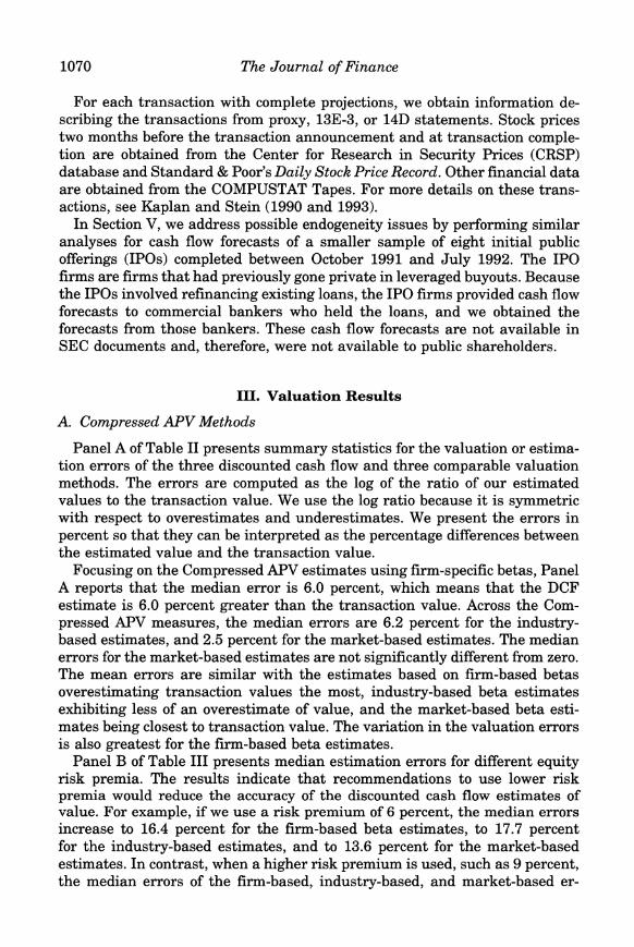
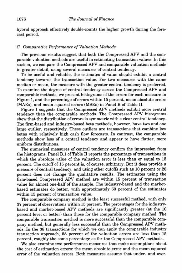
Figure 1. Distribution of valuation errors. Distribution of valuation errors for CAF'M-based and comparable-based valuation methods in 51 highly leveraged transactions completed between 1983 and 1989. The valuation errors equal the natural log of estimated values relative to transaction values. CAF'M-based values are the estimated present values of projected capital cash flows. Terminal values are grown a t 4 percent. Discount rates equal the long-term Treasury bond yield a t the time of the projections plus the equity risk premium times the relevant asset beta. The risk premium is the arithmetic average premium of the S&P 500 return over the long-term Treasury bond return from 1926 until the year before the transaction is announced. Estimated present values are calculated using (A) CAPM-based approach with firm asset betas; (B)CAPM-based approach with industry asset betas from value-weighted industry portfolios; (C) CAPM- based approach with market asset betas. Comparable values are calculated using (D) comparable company approach; (E)comparable transaction approach; and (F)comparable industry transaction approach (for which observations are limited to 38 transactions). The transaction value equals (1) market value of the firm common stock; plus (2)market value of firm preferred stock; plus (3) value of firm debt; plus (4) transaction fees; less (5) firm cash balances and marketable securities, all a t the time of the transaction. Debt not repaid in the transaction is valued a t book value; debt that is repaid, a t the repayment value.

The Valuation of Cash Flow Forecasts: A n Empirical Analysis 1075
CAPM with Firm Beta Comparable Company Method
I
I
0 0 0' 0 2 " 0 2 2 0 000 0 8
1 V a l ~ e Log ( E s t r a t e / V a ~ eLog ( E s t ~ ~ a t e : )
CAPM wlth Industry Beta Comparable Transaction Method
i
Log ( Estmate !Vaiue ;
CAPM wlth Market Beta Comparable Industry Transaction Method
I 7
1076 The Journal of Finance
hybrid approach effectively double-counts the higher growth during the fore- cast period.
C. Comparative Performance of Valuation Methods
The previous results suggest that both the Compressed APV and the com- parable valuation methods are useful in estimating transaction values. In this section, we compare the Compressed APV and comparable valuation methods in greater detail, using several measures of central tendency.
To be useful and reliable, the estimates of value should exhibit a central tendency towards the transaction value. For two measures with the same median or mean, the measure with the greater central tendency is preferred. To examine the degree of central tendency across the Compressed APV and comparable methods, we present histograms of the errors for each measure in Figure 1, and the percentage of errors within 15 percent, mean absolute errors (MAEs), and mean squared errors (MSEs) in Panel B of Table 11.
Figure 1suggests that the Compressed APV methods exhibit more central tendency than the comparable methods. The Compressed APV histograms show that the distribution of errors is symmetric with a clear central tendency. The firm-based and industry-based beta methods, however, have two and one large outlier, respectively. These outliers are transactions that combine low betas with relatively high cash flow forecasts. In contrast, the comparable methods show less of a central tendency and appear to have flatter, more uniform distributions.
The numerical measures of central tendency confirm the impression from the histograms. Panel B.l of Table I1 reports the percentage of transactions in which the absolute value of the valuation error is less than or equal to 15 percent. The cutoff of 15 percent is, of course, arbitrary. But it does provide a measure of central tendency, and using other cutoffs such as 10 percent or 20 percent does not change the qualitative results. The estimates using the firm-based Compressed APV method are within 15 percent of transaction value for almost one-half of the sample. The industry-based and the market- based estimates do better, with approximately 60 percent of the estimates within 15 percent of transaction value.
The comparable company method is the least successful method, with only 37 percent of observations within 15 percent. The percentages for the industry- based and market-based APV methods are significantly greater (at the 10 percent level or better) than those for the comparable company method. The comparable transaction method is more successful than the comparable com- pany method, but generally less successful than the Compressed APV meth-ods. In the 38 transactions for which we can apply the comparable industry transaction approach, 58 percent of the valuation errors are less than 15 percent, roughly the same percentage as for the Compressed APV methods.
We also examine two performance measures that make assumptions about the cost of estimation errors: the mean absolute error and the mean squared error of the valuation errors. Both measures assume that under- and over-

The Valuation of Cash Flow Forecasts: An Empirical Analysis 1077
valuations are equally costly. The MAE assumes that the cost of valuation errors increases linearly, while the MSE assumes that the cost increases are quadratic. Both measures are reported in panel B of Table 11, and both give qualitatively similar results. The MAE is 21.1 percent for the Compressed APV estimates using firm-based betas, 18.1 percent using industry-based betas, and 16.7 percent using market-based betas. The comparable methods have generally higher MAEs: 24.7 percent for the comparable company method; 18.1 percent for the comparable transaction method; and 20.5 percent for the comparable industry transaction method. The MAEs of the industry- and market-based APV methods are significantly smaller than the MAE of the comparable company method.
Finally, some readers might find it difficult to interpret these results in isolation. Accordingly, we compare the results for the Compressed APV method to those obtained in other financial applications. The obvious compar- ison is to models of option pricing. Whaley (1982) performs an analysis similar in spirit to ours for pricing American call options on dividend-paying stocks using variants of the Black-Scholes option pricing model. He finds mean prediction errors of 1.1 percent to 2.2 percent with standard deviations of 23.8 percent to 25.2 percent. These are qualitatively similar to those found for the Compressed APV methods, particularly the market-based method. In more recent work, Amin and Morton (1994) use six different models to price options on Eurodollar futures. Those models yield MAEs ranging from 15.2 percent to 21.1 percent which are, again, qualitatively similar to those obtained using the Compressed APV methods.
We conclude, based on the results presented in Tables I1 and 111, that the Compressed APV techniques provide a reasonable and accurate measure of value. The median errors are below 6.2 percent for all Compressed APV methods; the valuation errors have a strong tendency towards zero; and the valuation errors are qualitatively similar to those for option pricing models. The industry-based and market-based methods consistently perform better than the firm-based methods. The Compressed APV estimates using these two approaches perform about equally well.
Among the comparable methods, the comparable company method performs poorly. It is the least reliable valuation method we examine across all of the performance measures. The comparable transaction and the comparable in- dustry transaction methods both do better than the comparable company method, and work almost as well as the Compressed APV methods.
We favor the Compressed APV methods over the comparable methods for three reasons. First, the Compressed APV methods tend to have more valua- tion errors within 15 percent, and have lower MAEs and MSEs. Second, the comparable methods that work best are based on transactions, and therefore have little applicability beyond a transaction context. In contrast, the Com- pressed APV method can be used in a variety of corporate finance applications. This criticism is relevant even in the current sample for the comparable industry transaction method because that method fails to produce estimated values for more than one-quarter of the sample HLTs. Third, we think that, in

1078 The Journal of Finance
practice, participants are likely to have access to better estimates of cash flows and other inputs into the Compressed APV method than we have had available to us. On the other hand, we think that our information on comparables- especially on comparable transactions-is close to the information that would have been used in practice. There are potential improvements in the applica- tion of comparables, especially by making industry-specific choices of the type of multiple to apply. Nevertheless, we think the practical application of the Compressed APV method will improve its accuracy more than it will improve the comparable approaches.
D. Cross-Sectional Relation of Estimated Values to Transaction Values
The results in the previous sections focus on how well the Compressed APV and comparable valuation approaches estimate the actual transaction value level. I t is possible, however, that one of the approaches could successfully estimate the transaction value on average, yet perform poorly in explaining the variation in transaction values. The converse is also possible. In this section, we consider these possibilities by estimating regressions to deter- mine how well the different valuation methods explain the variation in transaction values. With a regression approach, we can also test whether using the DCF and comparable approaches together can explain additional variation.
The regressions relate transaction values to estimated values from the Com- pressed APV and comparable methods. The basic model we want to estimate is:
Transaction Value = a + p Estimated Value + E ( 5 )
If the estimated values are unbiased predictors of transaction value, the coeffi- cient estimates for the intercept will be zero and for the slope, will be one. Because it seems likely that the intercept term and the error term will be related to value or size, we consider two specifications of the model. First, we regress the log of transaction value on the log of estimated value. Second, we eliminate size entirely by regressing the transaction value as a multiple of EBITDA on estimated value, again expressed as a multiple of EBITDA.
Column 1of Table IV presents the regression results for the log-log specifica- tion. The estimates from the three Compressed APV approaches in Column 1are consistent with the approach providing unbiased estimates of transaction values. The intercepts are all insignificantly different from zero, and the slopes are all insignificantly different from one. The F-statistics of the joint test (intercept equal to zero and slope equal to one) are insignificant for all three methods. Furthermore, the estimated values explain virtually all the variation in transaction values and the residuals from the log-log specification are well-behaved-there is no evidence of heteroscedasticity or undue influence from large observations.

The Valuation of Cash Flow Forecasts: A n Empirical Analysis 1079
Table IV
Cross-Sectional Relation of Estimated Values to Transaction Values Regressions of transaction values on estimated net present values in 51 highly leveraged trans- actions completed between 1983 and 1989. Regressions using multiples include transaction values and estimated net present values as multiples of EBITDA (earnings before interest, taxes, depreciation, and amortization) in the year before the transaction. Estimated net present values are calculated using (A) Capital Asset Pricing Model (CAPMI-based approach with firm asset betas; (B) CAPM-based approach with industry asset betas from value-weighted industry portfo- lios; (C) CAPM-based approach with market asset betas; (D) comparable company approach; and (El comparable transaction approach. All CAPM-based approaches use a terminal value growth rate of 4 percent. Transaction value equals (1) the market value of the firm common stock; plus (2) the market value of firm preferred stock; plus (3) the value of the firm debt; plus (4) transaction fees; less (5) firm cash balances and marketable securities, all a t the time of the transaction. Debt not repaid in the transaction is valued at book value; debt that is repaid, a t the repayment value. Standard errors are in parentheses. Dependent variable is transaction value or transaction value as a multiple of prior year EBITDA.
Regressions of Logs Regressions of Levels
1. 2. 3. 4. 5. 6. Univariate Combined Univariate Combined Univariate Combined
Estimated Regressions Regression Regressions Regression Regression Regressions Values (Logs) (Logs) (Multiples) (Multiples) (Multiples) (Multiples)
Panel A. Firm Beta
Constant 0.06 (0.21) 1.25" (0.18) 5.50" (0.80) Slope 0.98* (0.03) 0.39" (0.08) 0.32" (0.08)
R2 = 0.95 R2 = 0.33 R" 0 2 4
Panel B: Industry Beta
Constant 0.05 (0.19) 1.10" (0.17) 4.85" (0.73) Slope 0.98" (0.03) 0.46* (0.08) 0.39* (0.07)
R2 = 0.96 R2 = 0.43 R2 = 0.36
Panel C: Market Beta
Constant 0.22 (0.17) 0.21 (0.13) 1.06" (0.19) -0.16 (0.66) 3.82" (0.88) -1.46 (2.69) Slope 0.97" (0.03) 0.35" (0.10) 0.50" (0.09) 0.36* (0.10) 0.55" (0.10) 0.34" (0.11)
R2 = 0.97 R2 = 0.39 R2 = 0.39
Panel D: Comp. Company
Constant 0.55* (0.17) 1.28" (0.23) 4.51" (0.82) Slope 0.94" (0.03) 0.28" (0.09) 0.43* (0.12) 0.29" (0.11) 0.55" (0.11) 0.40" (0.11)
R2 = 0.96 R2 = 0.22 R2 = 0.34
Panel E: Comp. Transaction
Constant 0.21 (0.16) 0.39 (0.77) 1.40 (3.49) Slope 0.97" (0.02) 0.35" (0.11) 0.82** (0.36) 0.46 (0.31) 0.85"" (0.42) 0.50 (0.33)
R2 = 0.97 R2 = 0.98 R2 = 0.09 R2 = 0.48 R2 = 0.08 R2 = 0.53
No. of 51 51 51 51 51 51 observations
" and ** denote significant difference from zero a t the 1and 5 percent level, respectively.

1080 The Journal of Finance
Again, the Compressed APV methods perform at least as well as the compara- ble methods. The comparable value methods explain a similar amount of variation in transaction value. However, in the comparable company regression, the inter- cept is different from zero and the slope coefficient is different from one. The joint F-test of an intercept of zero and slope of one is strongly rejected.8
In some sense, however, the DCF and comparable approaches are too suc- cessful in explaining the vahation in transaction values using the log-log specification. Although the residuals in the regressions are well-behaved, the log-log specifications may perform so well because they regress measures of size on size. For the second set of regressions, we eliminate size by scaling transaction values and estimated values by EBITDA in the year before the transaction. We then regress the resultant transaction value multiples on the estimated value multiples:
Transaction Value Multiple = cu + P Estimated Value Multiple + E (6)
This specification is particularly attractive because, typically, the comparable estimates were calculated and HLT values were reported as multiples of EBITDA. (See Kaplan (198913) and DeAngelo (1990)).
Table IV presents results of both log-log and level-level specifications for these scaled regressions. Again, we prefer the log-log specification because it assumes a more reasonable multiplicative error structure.9 In Column 3, the estimates from the APV approaches explain from 33 percent to 43 percent of the variation in transaction multiples. The industry-based approach explains the most variation; the firm-based approach, the least. In contrast, the com- parable company and comparable transaction multiples explain much less variation, at 22 percent and 9 percent, respectively. Although not reported, the comparable industry transaction multiples explain only 5 percent of the vari- ation. Column 5 indicates that the industry-based and market-based APV approaches also explain more variation than both of the comparable ap- proaches in the level-level specification.
While they explain an impressive amount of variation in transaction multi- ples, there is one respect in which the Compressed APV multiples (as well as the comparable company multiples) are disappointing. The constant terms in the regressions differ significantly from zero, and the slope coefficients differ significantly from one. All of the valuation methods tend to overvalue high multiple transactions and undervalue low multiple transactions. While the
We do not present regressions using the comparable industry transaction estimated values because the regressions include only 38 observations and because those values explain less variation in transaction value than the other two comparable methods.
We obtain economically and statistically similar results to the log-log specification when we regress the log of the transaction values on the log of the estimated values and the log of EBITDA.

The Valuation of Cash Flow Forecasts: A n Empirical Analysis 1081
comparable transaction method performs best on this dimension, it explains by far the least variation in transaction multiples.lo
Overall, the univariate regression results indicate that the APV approaches perform well relative to the comparable approaches in explaining variation in transaction values and multiples. The APV approaches are individually supe- rior to the comparable approaches in explaining the variation in transaction multiples. We interpret these results as additional evidence in favor of the usefulness of the discounted value approaches. Choosing among the three APV methods, the industry-based and market-based approaches outperform the firm-based approach in explaining variation in transaction values as they did in predicting the level of the transaction value.
The previous discussion compares the APV and comparable methods against each other. It is possible, however, that the different valuation approaches contain different information about transaction values. Accordingly, column 2 of Table IV presents estimates from a regression that includes the market- based Compressed APV values, the comparable company values, and compa- rable transaction values as independent variables in the original, nonscaled specification. All three variables are statistically significant, the intercept term is not significantly different from zero, and the variables together explain more variation in transaction value than any one of them does alone. We cannot reject the joint hypothesis that the intercept is zero and the sum of the slope coefficients equals one.
Columns 4 and 6 present the results of regressions that include the market- based APV multiples, the comparable company multiples, and the comparable transaction multiples in log-log and level-level specifications. The APV and comparable multiples together explain roughly 50 percent of the variation in transaction multiples. The coefficients indicate that the APV and comparable company methods both have significant explanatory power for transaction multiples. Although the comparable transaction multiple has the largest coeffi- cient, that coefficient is not significant. Again, we cannot reject the joint hypoth- esis that the intercept is zero and the sum of the slope coefficients equals one.
loOne possible explanation for the slope terms being less than one is that the constant term measures the contribution of EBITDA in explaining transaction value. This can be seen by multiplying equation (6) by EBITDA to recast the regression in levels:
Transaction Value = a EBITDA + P Estimated Value + E ' (6')
If the estimated values are measured with some error, and EBITDA is correlated with the estimated values, a in equation (6)will not equal zero, and /3 will not equal one. We also estimated the reverse regressions in which the transaction value is the independent value and the estimated values are the dependent variables. In those regressions, only one slope coefficient in the APV estimate reverse regressions-that using the market-based APV values-differs significantly from one, a t the 10 percent level, whereas the slope coefficients in all of the comparable estimate reverse regressions do. This explanation implies that the log-log value specification in equation (5) also should have measurement error. Consistent with this, the slope coefficients in reverse regressions of equation ( 5 ) tend to be closer to one than the slope coefficients in the forward regressions, even though most of the coefficients in both sets of regressions do not differ signifi- cantly from one.

1082 The Journal of Finance
The regression results in columns 2, 4, and 6 indicate that when feasible, it is worthwhile to combine the information in the APV and comparable approaches.
IV. Implied Cost of Capital
In this section, we revisit the risk premium that is used in our Compressed APV calculations. We devote special attention to the risk premium because there is substantial debate about how the risk premium should be measured. Some rely on the method we prefer which is a long-term arithmetic average of the historical return spread between a stock market index and riskless bonds-e.g., Brealey and Myers (1991). Others argue for a geometric aver- age-e.g., Copeland, Koller, and Murrin (1990). These methods provide sub- stantially different measures of risk premia. For example, the geometric average spread is 5.41 percent, which is roughly 2 percent below the median arithmetic average spread we use of 7.42 percent.
We invert our analysis to derive the discount rates implied by the transac- tion values to provide direct empirical evidence about the risk premium. We use the same forecast capital cash flows and terminal values to calculate an implied discount rate or cost of capital that equates the estimated value to the transaction value. The implied risk premium equals the difference between the implied discount rate and the yield on long-term Treasury bonds at the time of the projections. The implied risk premium represents the product of the implied market equity risk premium and an asset beta. We estimate an implied market equity risk premium by dividing the implied risk premium by our market-based asset beta (where the market-based asset beta is calculated using the value weighted capital structure for nonfinancial, nonutility firms in the S&P 500 in the fiscal year before the HLT announcement).
A. Implied Discount Rates, Risk Premia, and Market Equity Risk Premia
Using our assumption of 4 percent growth in calculating terminal values, Table V reports that the median implied discount rate for the 51 HLTs is 15.77 percent, the mean is 16.28 percent, and the standard deviation is 2.69 percent. The implied risk premium, calculated by subtracting the contemporaneous long-term Treasury bond yield, has a median of 7.08 percent, a mean of 7.14 percent, and a standard deviation of 2.87 percent. The median implied market equity risk premium is 7.78 percent, the mean is 7.97 percent, and the stan- dard deviation is 3.30 percent. We do not find any variation over time in the implied market equity risk premia. Admittedly, such variation might be hard to detect, given the clustering of our sample in the late 1980s.
Table V also presents implied discount rates, risk premia, and market equity risk premia assuming terminal value growth rates of 6 percent, 2 percent, and 0 percent. Not surprisingly, the risk premia vary with the terminal value growth rate. The median implied market equity risk premium drops to 5.60 percent with no terminal value growth and increases to 9.03 percent with 6

The Valuation of Cash Flow Forecasts: A n Empirical Analysis 1083
Table V
Implied Discount Rates, Risk Premia, and Market Equity Risk Premia
Discount rates, risk premia, and market equity risk premia implied by projected capital cash flows in 51 highly leveraged transactions completed between 1983 and 1989. Terminal growth rate assumed to grow a t 4 ,6 ,2 , and 0 percent. The transaction value equals (1)the market value of the firm common stock; plus (2) the market value of firm preferred stock; plus (3)the value of the firm debt; plus (4)transaction fees; less (5)firm cash balances and marketable securities, all a t the time of the transaction. Debt not repaid in the transaction is valued at book value; debt that is repaid, a t repayment value. The implied discount rate discounts the capital cash flows to a value equal to the transaction value. The implied risk premium equals the difference between the implied discount rate and the yield on long-term Treasury bonds (from Ibbotson Associates) a t the time of the projections. The implied market equity risk premium uses the value weighted capital structure for nonfinancial, nonutility firms in the S&P 500 in the fiscal year before the highly leveraged transaction announcement to transform the implied risk premium into the risk premium for an investment with a beta of one.
Terminal Value Std. Interquart. Growth Rate (%) Median Mean Dev. Range Min. Max. N
Panel A: Implied Discount Rate
4 15.77 16.28 2.69 3.06 10.37 24.16 51
6 16.77 17.32 2.64 2.80 11.55 25.39 51 2 14.85 15.29 2.75 3.24 9.29 23.16 51 0 13.79 14.36 2.83 3.50 8.29 22.46 51
Panel B. Implied Risk Premium
Panel C. Implied Market Equity Risk Premium
percent terminal value growth. As we noted earlier, we feel that a 4 percent growth rate is the economically most plausible assumption.
Like the evidence in Section 111, the risk premium results strongly suggest that the Compressed APV technique works best when an arithmetic average risk premium is used. The estimated market equity risk premium of 7.78 percent is remarkably close to the (median 7.42 percent) long-term arithmetic average return spread between the S&P 500 index and long-term Treasury bonds that we use for our Compressed APV estimates. There is no evidence that the use of lower risk premia, however obtained, would improve the accuracy of discounted cash flow techniques.

1084 The Journal of Finance
B. Relation of Implied Risk Premia to Systematic Risk, Size, and Book-to-Market
In this section, we examine the relation between our implied risk premia and 1)firm asset betas; 2) industry asset betas; 3) transaction size; and 4) company book-to-market ratios (in the fiscal year ending before the transaction is announced). Our examination is motivated by two findings. First, Fama and French (1992) report that equity returns are negatively related to firm size, positively related to the book-to-market ratio, but unrelated to equity betas. Second, the results reported in Section I11 indicate that the Compressed APV method using market-based betas works about as well as industry-based and better than firm-based betas. Both of these results are contrary to the gener- ally accepted notion that expected returns are related to systematic risk. By examining the determinants of the individual implied risk premia in our sample, we provide evidence on how the market determines expected returns. We use pre-transaction book-to-market ratios because at the time the transaction is completed, book-to-market ratios equal one for all management buyouts and are typically negative for recapitalizations. (The book-to-market analyses exclude observations with negative pretransaction book-to-market ratios.)
Table VI presents univariate regressions of the risk measures on the implied risk premium. The regressions indicate that the implied risk premium is positively related to both beta measures. In the two univariate regressions, however, neither of the coefficients on the betas is statistically significant at the 10 percent level. The insignificance of the regression coefficient for the industry beta appears to be caused by outliers. Nonparametric rank tests indicate that the risk premium is significantly related to industry betas (at the 10 percent level). We also find a significant relation-both parametrically and nonparametrically-between the implied risk premia and the original, levered industry equity betas.
While the risk premia are marginally related to industry betas, Table VI indicates that the implied risk premia are unrelated to firm size-(the log of) transaction value-or to the prebuyout book-to-market ratio. Nonparametric rank correlations also fail to identify any significant relation between the risk premium and either size or the book-to-market ratio.
The patterns are qualitatively similar when beta, size, and book-to-market ratios are included in the same regression. In fact, the firm asset beta becomes significant at the 10 percent level in the multiple regression. Overall, these results suggest a positive relationship between expected returns and system- atic or beta risk, but provide no basis for concluding that discounted cash flow valuations could be improved by basing discount rates on firm size or market- to-book ratios.11
Because the sample period precedes the Fama-French paper, i t is possible to argue that the Fama-French factors do not matter because practitioners used the wrong discount rates. Although possible, we find this unpersuasive. After all, early tests of the CAPM used return data from periods that preceded the CAPM's formulation.

The Valuation of Cash Flow Forecasts: A n Empirical Analysis 1085
Table VI
Relation of Implied Risk Premium to Systematic Risk and Size The implied risk premium is the risk premium implied by projected capital cash flows in 51 highly leveraged transactions (HLT) completed between 1983 and 1989. The terminal value is assumed to grow at 4 percent. The transaction value equals (1)the market value of the firm common stock; plus (2) the market value of firm preferred stock; plus (3) the value of the firm debt; plus (4) transaction fees; less (5) firm cash balances and marketable securities, all a t the time of the transaction. Debt not repaid in the transaction is valued at book value; debt that is repaid, a t the repayment value. The implied discount rate discounts the capital cash flows to a value equal to the transaction value. The implied risk premium equals the difference between the implied discount rate and the yield on long-term Treasury bonds at the time of the projections. Firm equity betas are calculated using the method in Dimson (1979). Firm asset betas are calculated using the firm equity, preferred, and debt betas, and preannouncement capital structures. Industry asset betas are calculated by applying the industry equity, preferred, and debt betas to the value-weighted capital structure for industry firms in the fiscal year before the HLT announcement. Industry- specific equity betas are calculated using value-weighted portfolio returns of firms in the same two-digit SIC code as the HLT firm. Equity betas are calculated over the period 540 to 60 trading days before the HLT announcement. For all calculations, preferred stock and debt betas are assumed equal to 0.25. Log size equals the log of the transaction value. Book-to-market is the ratio of company book value of equity plus deferred taxes to the market value of equity in the year ending before the transaction.
Dependent Variable is Implied Risk Premium (in 70)
Constant
Firm asset beta
Industry asset beta (portfolio-based)
Log size
", "", and *"" denote significant difference from zero a t the 1, 5, and 10 percent level, respectively.
V. Potential Endogeneity or Hardwiring of Cash Flow Forecasts
The previous sections indicate that the Compressed AF'V valuation ap- proaches provide reasonably accurate estimates of transaction values. This is somewhat surprising because the high levels of debt in HLTs provide signifi- cant valuation challenges. The success of the Compressed APV approaches in valuing these complex HLTs raises the question of whether there is something special about our sample of HLTs that makes the Compressed AF'V technique so effective, and whether there are reasons to doubt that the AF'V methods will work as well in practice as they do in our tests.

1086 The Journal of Finance
The primary concern is that the cash flows might somehow be endogenous, and that the endogeneity causes the Compressed APV valuations to be spuri- ous estimates of transaction value. One potential source of endogeneity is that dealmakers and managers in the HLTs in our sample may have had incentives to adjust the cash flow forecasts.12 If the transaction value and financial structure are determined by competition in the market for corporate control, dealmakers may have an incentive to construct their cash flow forecasts to justify the price and to convince lenders and investors to finance the transac- tions. The transaction value and financial structure imply a sequence of required interest and principal payments, and the forecast cash flows have to exceed those debt payments for the transaction to be feasible. Because the sample transactions are largely debt financed (a median 88 percent of trans- action value), cash flows that are constructed to exceed debt payments would be "hardwired in the sense that cash flows are constructed so that their present value will yield the transaction value.
One implication of hardwiring is that the cash flow forecasts are adjusted upward or downward to approximate the required debt payments. Incentives to bias the cash flow forecasts upward may occur when true expected cash flows are below the level required to obtain financing. Incentives to bias the cash flows downward may occur when the true expected cash flows are sub- stantially in excess of those required to obtain financing. Because the SEC and courts require the HLT firm's board of directors to obtain an opinion from an investment bank that the transaction value is "fair," insiders and dealmakers may have an incentive to reduce their reported cash flow forecasts to justify the transaction value.
As an illustration of hardwiring, consider a typical HLT that finances 55 percent of transaction value with bank debt at a nominal rate that exceeds the Treasury bond rate by 1.5 percent; approximately 35 percent of transaction value with subordinated debt at a nominal rate that exceeds the Treasury bond rate by 4.5 percent; and approximately 10 percent of transaction value with equity at an unknown rate of return over the Treasury bond. Assuming that equity yields a nominal return at least 4.5 percent over the Treasury bond, hardwiring would put a lower bound on the internal rate of return equal to the Treasury bond yield plus 2.85 percent.
The Treasury bond yield plus 2.85 percent is substantially below the implied discount rate (the Treasury bond yield plus 7.08 percent) that we estimate in Section IV, suggesting that our basic empirical findings are not confounded by hardwiring. Furthermore, hardwiring implies that all parties-investors, courts, investment banks, etc.-use methods like Compressed APV to deter- mine the transaction value. Although we doubt that the Compressed APV
For example, although it is not in our sample, there is some evidence that the managers at Interco made such adjustments during the financing of their leveraged recapitalization. See Jereski (1991). See also Burrough and Helyar (1990) for a description of how cash flows were forecast in the FUR Nabisco buyout.

The Valuation of Cash Flow Forecasts: A n Empirical Analysis 1087
method works simply because everyone uses it, we take the hardwiring criti- cism seriously and perform four sets of tests for evidence of hardwiring.
A. Ex post Accuracy of Cash Flow Forecasts
If the forecast cash flows are biased either upward or downward, there should be differences between the forecasts and the realizations. This is difficult to test because we know of no method to directly measure the ex ante bias, if any, in the forecasts. We rely, therefore, on ex post data to gauge the accuracy of the forecasts. Using ex post data to assess the forecasts is, however, complicated because the U.S. economy entered a recession in 1990, less than two years after the majority of these transactions. The forecasts were unlikely to anticipate the recession and thus, even if the forecasts were unbiased ex ante estimates of expected cash flows, we anticipate that the forecasts will exceed the actual cash flows. Nevertheless, we examine the ex post accuracy of the projections by comparing forecast EBITDA to post-transaction EBITDA. We also examine EBITDA margins-the ratio of EBITDA to sales-because the recession as well as asset sales not considered in the projections should have had less effect on margins.
We are able to obtain at least one year of post-transaction data for 46 of the 51 sample HLTs. In the first and second complete fiscal years after the HLT, EBITDA levels are, respectively, a median of 3.7 percent and 14.4 percent below those forecast, both of which are statistically significant at the 5 percent level. This is consistent with optimistic cash flow forecasts caused by either ex ante optimism or an unanticipated recession. In contrast, we find only weak evidence that forecast EBITDA margins are biased. EBITDA margins are below those forecast by a median of 3.2 percent and 3.6 percent of the forecast margin, respectively, in the first and second years after the transaction. (If EBITDA margins were forecast to equal 20.0 percent of sales, a 3.6 percent shortfall in margins is equivalent to actual margins being 19.3 percent of sales.) The shortfall in the first year is statistically insignificant, while the second year shortfall is significant only at the 10 percent level. The EBITDA and EBITDA margin shortfalls are also smaller than those documented in Kaplan (1989a) for an earlier sample of management buyouts. Overall, there- fore, there is some evidence of optimistic EBITDA forecasts. But the closeness of the forecast and realized EBITDA margins suggests that at least some of the difference between forecast and actual EBITDA is related to the unanticipated recession instead of an ex ante bias.
B. Leverage
If cash flows forecasts are hardwired to repay debt, the hardwiring effect and the accuracy of the Compressed APV approaches should be more pronounced in more highly leveraged transactions. We test this implication of hardwiring by dividing the sample into firms that have above- and below-median post- transaction leverage (i.e., debt to transaction value). If hardwiring is causing

1088 The Journal of Finance
our results, the Compressed APV techniques should be more accurate for the high debt subsample.
Using the market-based APV approach, the mean absolute error for the lower debt sample is 17.1 percent of transaction value compared to 16.7 percent for the higher debt sample; and the mean squared error for the lower debt sample is 5.07 percent compared to 5.17 percent for the higher debt sample. Furthermore, the Compressed APV estimates (as multiples of EBITDA) for the lower debt sample explain more variation in (log) transaction multiples than the estimates for the higher debt sample-46 percent of the variation versus 28 percent. The only evidence consistent with the hardwiring explanation is that estimated values are within 15 percent of transaction value for 52 percent of the low debt sub-sample and 65 percent of the high debt sub-sample. And even this difference is not significant. Overall, these results do not provide much evidence for hardwiring.
C. Initial Public Offerings
In this section, we again test the hardwiring implication that the Com- pressed APV approaches should be less accurate for less highly-leveraged companies by estimating the value of firms in initial public offerings.
The IPOs are also particularly interesting because the incentives to hard- wire the forecasts in IPOs are different from those in HLTs. We have noted that there may be incentives in HLTs to bias cash flows upward-to obtain financing-or to bias cash flows downward-to obtain a fairness opinion. In the IPOs in our sample, there are similar incentives to raise forecasts, but-unlike HLTs-there are no incentives to lower forecasts. The key difference is that the forecasts for the IPOs were provided to banks as part of the process of refinancing the HLT bank loans, but were not made available to equity investors. Unlike HLTs, if managers of an IPO firm believe future cash flows are going to be very strong, they do not require a fairness opinion and, therefore, have no incentive to present cash flow forecasts that are lower than they believe. Like HLTs, however, managers of an IPO firm might have an incentive to present cash flow forecasts that are higher than they believe in order to ensure financing and potentially get a higher IPO valuation. If hardwiring and associated incentives are causing spurious results in our HLT sample, the Compressed APV techniques should be higher and less accurate for the IPOs.
We obtained detailed cash flow forecasts for eight IPOs completed between October 1991 and July 1992. The IPOs all involved refinancing of existing debt because the eight issuers were companies that had previously completed highly leveraged transactions. We calculate the transaction value using the closing stock price on the day of the IPO.l3 Based on this price, the median
l3 By using the closing stock price, we avoid any bias that might be introduced by underpricing. This is probably a nonissue for this sample because the equity underpricing is very small-a median of 0.5 percent and an average of 2.3 percent.
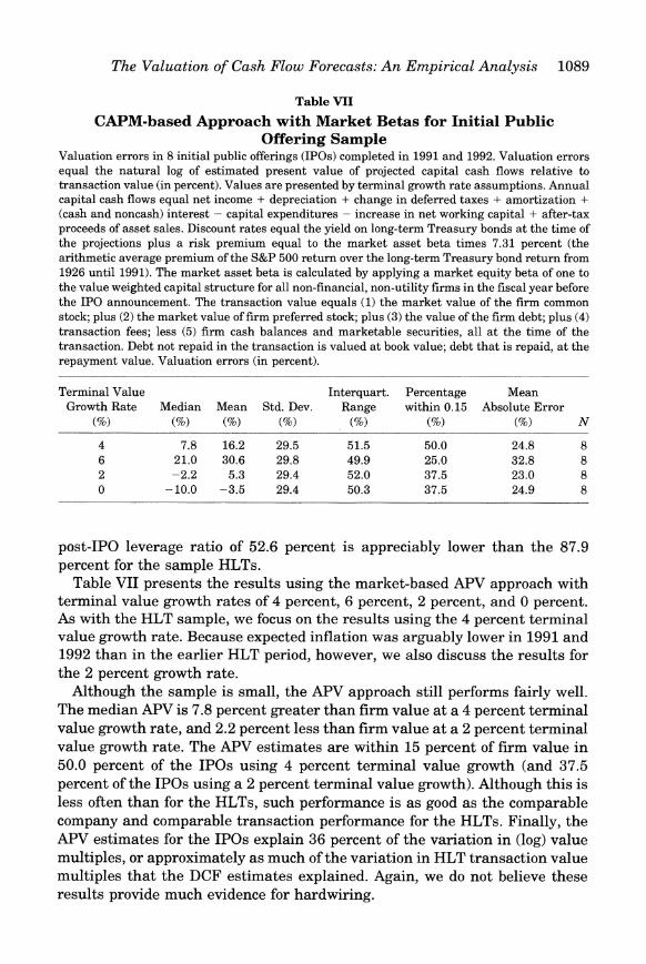
The Valuation of Cash Flow Forecasts: A n Empirical Analysis 1089
Table VII
CAPM-based Approach with Market Betas for Initial Public Offering Sample
Valuation errors in 8 initial public offerings (IPOs) completed in 1991 and 1992. Valuation errors equal the natural log of estimated present value of projected capital cash flows relative to transaction value (in percent). Values are presented by terminal growth rate assumptions. Annual capital cash flows equal net income + depreciation + change in deferred taxes + amortization + (cash and noncash) interest - capital expenditures - increase in net working capital + after-tax proceeds of asset sales. Discount rates equal the yield on long-term Treasury bonds at the time of the projections plus a risk premium equal to the market asset beta times 7.31 percent (the arithmetic average premium of the S&P 500 return over the long-term Treasury bond return from 1926 until 1991). The market asset beta is calculated by applying a market equity beta of one to the value weighted capital structure for all non-financial, non-utility firms in the fiscal year before the IPO announcement. The transaction value equals (1) the market value of the firm common stock; plus (2) the market value of firm preferred stock; plus (3) the value of the firm debt; plus (4) transaction fees; less (5) firm cash balances and marketable securities, all a t the time of the transaction. Debt not repaid in the transaction is valued at book value; debt that is repaid, a t the repayment value. Valuation errors (in percent).
Terminal Value Interquart. Percentage Mean Growth Rate Median Mean Std. Dev. Range within 0.15 Absolute Error
(5%) (5%) (%I (5%) (%) (5%) (5%) N
post-IPO leverage ratio of 52.6 percent is appreciably lower than the 87.9 percent for the sample HLTs.
Table VII presents the results using the market-based APV approach with terminal value growth rates of 4 percent, 6 percent, 2 percent, and 0 percent. As with the HLT sample, we focus on the results using the 4 percent terminal value growth rate. Because expected inflation was arguably lower in 1991 and 1992 than in the earlier HLT period, however, we also discuss the results for the 2 percent growth rate.
Although the sample is small, the APV approach still performs fairly well. The median APV is 7.8 percent greater than firm value at a 4 percent terminal value growth rate, and 2.2 percent less than firm value at a 2 percent terminal value growth rate. The AF'V estimates are within 15 percent of firm value in 50.0 percent of the IPOs using 4 percent terminal value growth (and 37.5 percent of the IPOs using a 2 percent terminal value growth). Although this is less often than for the HLTs, such performance is as good as the comparable company and comparable transaction performance for the HLTs. Finally, the APV estimates for the IPOs explain 36 percent of the variation in (log) value multiples, or approximately as much of the variation in HLT transaction value multiples that the DCF estimates explained. Again, we do not believe these results provide much evidence for hardwiring.

1090 The Journal of Finance
D. Contested and Uncontested HLTs
Incentives to raise a cash flow forecast to justify a transaction ought to be higher when there are other bidders or some other form of outside pressure. In such situations, the failure to finance and complete the HLT both increases the likelihood that incumbent managers will lose their jobs (to the winning bidder) and ensures that dealmakers will lose their transaction fees. This suggests that in transactions that involve multiple bidders or hostile pressure, forecast cash flows ought to be higher relative to true "expected" cash flows. If this is the case, ex post performance relative to the forecasts ought to be lower. One might also argue that the APV estimates ought to be closer to the transaction values-i.e., have smaller MAEs and MSEs-when there is hostile pressure. We find little support for these two hypotheses.
In our sample, 18 firms explicitly received competing bids and 6 additional firms experienced hostile pressure in the form of block share purchases by outside parties for a total of 24 firms with some form of outside pressure. There was no overt outside pressure for 27 transactions. The valuation errors are insignificantly different across the two subsamples. Using a market-based APV approach (with 4 percent terminal value growth), the median APV esti- mate is 4.0 percent above the transaction value (mean is 1.3 percent) when there is outside pressure, and 0.6 percent below the transaction value (mean is 4.7 percent) when there is not. The Compressed APV estimates are more accurate, but insignificantly so, when there is outside pressure. For example, the mean absolute error for the outside pressure sample is 14.9 percent compared to 18.7 percent for the nonhostile sample. Also, 62.5 percent of the outside pressure APV estimates are within 15 percent of transaction value compared to 55.6 percent of the APV estimates with no outside pressure.
Most importantly, when we compare the ex post performance of the two subsamples of HLTs to the cash flow forecasts, we find no significant differ- ences in EBITDA or EBITDA margins. In the first and second post-transaction years, respectively, EBITDA levels are a median of 9.5 percent and 13.6 percent below those forecast for the outside pressure transactions, and 2.8 percent and 20.5 percent below those forecast for the transactions with no outside pressure. Similarly, EBITDA margins are a median of 6.1 percent and 2.6 percent below those forecast for the outside pressure transactions, and 2.0 percent and 4.6 percent below those forecast for the transactions with no outside pressure. Again, we do not believe these results provide much evidence for hardwiring.
E. Discussion
None of the four sets of tests provide much evidence for the predictions of hardwiring. In our view, there is no reason to believe that the reliability of the Compressed APV methods is spurious. However, without ex ante evidence that the cash flow forecasts are actually an estimate of expected cash flows, we cannot completely eliminate the possibility that dealmakers systematically and materially adjusted their cash flow forecasts. While there may have been

The Valuation of Cash Flow Forecasts: A n Empirical Analysis 1091
other pressures or incentives that we have not examined, we have shown that the most obvious (at least to us) possible biases in the forecasts do not receive strong support from our data.
There are several reasons that adjustments to cash flows, especially larger ones, are costly. First, most of the dealmakers and investors in a particular HLT could expect to meet again in a future transaction. There were undoubt- edly some reputational incentives not to present fictional forecasts. Second, in transactions that ultimately fail, creditors can sue insiders under fraudulent conveyance law if the original transaction rendered the company insolvent (solvency test) or the company had unreasonably small capital, i.e., insufficient forecast cash flow to meet debt payments (capital test). Both tests rely on the cash flow forecasts made at the time of the transaction. Courts and their examiners in fraudulent conveyance hearings have paid careful attention to whether the cash flow forecasts were "reasonable." (See Baird (1991) for a description of fraudulent conveyance law.) The failure of the Interco recapi- talization received such an unusual amount of attention precisely because the cash flow forecasts were considered to have been unreasonable.
Furthermore, academic and anecdotal evidence suggest that bankers and buyout specialists took the cash flow forecasts seriously. Anders (1992) writes that the projections "took on a stature that was both awesome and terrifying to top executives. Unlike budgets that executives devised, the bank-book projections were ironclad." (Denis and Denis (1993) provide quantitative evi- dence that firms in recapitalizations were constrained by such budgets.) At a minimum, managers could expect that failure to meet those projections would bring increased scrutiny and pressure from banks and investors. To the extent that missed projections are followed by missed debt payments, equity investors could expect to lose their investment and managers could expect to lose their investment and their jobs.
It is, of course, possible that the Compressed APV methods succeed because all market participants were making the same mistakes. In particular, mis- takenly high forecast cash flows may have mapped well into mistakenly high transaction values. (Kaplan and Stein (1993) present evidence consistent with the HLT market having overheated during the sample period.) There are two reasons that we are less concerned by this possibility. First, even if everyone were mistaken, it would not alter the fact that the Compressed APV methods are relatively successful and useful in predicting contemporaneous market values. Second, the roughly similar success of the Compressed APV methods in predicting IPO market values during a very different period supports the general reliability of those methods.
VI. Summary
This study provides evidence that discounted cash flow valuation methods provide reliable estimates of market value. Our median estimates of dis- counted cash flows for 51 HLTs are within 10 percent of the market values of the completed transactions and perform at least as well as valuation ap-

1092 The Journal of Finance
proaches using companies in similar industries and companies involved in similar transactions. We stress that our estimates rely on a number of ad hoc assumptions that readers (both academics and practitioners) should be able to improve on. We would expect such improvements to bring the DCF valuations even closer to the transaction values.
We use three CAPM-based approaches to estimate discount rates corre- sponding to firm-level, industry-level, and market-level measures of risk. All three methods perform well compared to those using comparable transactions and companies. Under what we consider the most realistic assumptions, the industry- and market-based approaches perform best. Although the DCF ap- proaches perform at least as well as the comparable-based approaches, we find that the comparable-based estimates add explanatory power to the DCF-based estimates. Accordingly, we would recommend using information from both types of approaches in practical valuation settings where comparable values are available.
In the second part of this article, we use the forecast cash flows and trans- action values to calculate implied discount rates and risk premia. The median implied market equity risk premium, the amount by which the return on the equity market exceeds the long-term Treasury bond yield, equals 7.78 percent. This accords well with the historical risk premium by which returns on the S&P 500 have exceeded Treasury bond returns. The relations between the implied risk premia and both firm and industry betas are positive and mar- ginally significant. In contrast, there are no apparent relations between the implied risk premia and either transaction value, i.e., firm size, or book-to- market ratios. For this sample, therefore, the results favor CAPM-based ap- proaches to discount rates over those based on size or book-to-market ratios.
REFERENCES
Arnin, Kaushik, and Andrew Morton, 1994, Implied volatility in term structure models, Journal of Financial Economics 35, 141-180.
Anders, George, 1992, Merchants of Debt. (Basic Books, New York). Baird, Douglas, 1991, Fraudulent conveyances, agency costs, and leveraged buyouts, Journal of
Legal Studies 20, 1-25. Blanchard, Olivier, 1993, Movements in the equity premium, Brookings Papers on Economic
Activity 2, 75-138. Blume, Marshall, 1975, Betas and their regression tendencies, Journal of Finance 30, 785-795. Brealey, Richard, and Stewart Myers, 1991, Principles of Corporate Finance. (McGraw-Hill, New
York, 4th Edition). Burrough, Bryan, and John Helyar, 1990, Barbarians at the Gate. (Harper and Row, New York). Copeland, Tom, Tim Koller, and Jack Murring, 1990, Valuation. (John Wiley & Sons, New York). Cornell, Bradford, and Kevin Green, 1991, The investment performance of low-grade bond funds,
Journal of Finance 46, 29-48. DeAngelo, Linda, 1990, Equity valuation and corporate control, The Accounting Review 65,
93-112. Denis, David, and Diane Denis, 1993, Managerial discretion, organizational structure, and cor-
porate performance: A study of leveraged recapitalizations, Journal of Accounting and Eco- nomics 16, 209-236.
Dimson, Elroy, 1979, Risk measurement when shares are subject to infrequent trading, Journal of Financial Economics 7, 197-226.

The Valuation of Cash Flow Forecasts: A n Empirical Analysis 1093
Fama, Eugene, and Kenneth French, 1992, The cross-section of expected stock returns, Journal of Finance 47, 427-466.
Ibbotson Associates, 1991, Stocks, Bonds, Bills, and Inflation 1991 Yearbook, (Ibbotson Associates, Inc., Chicago).
Jereski, Laura, 1991, Fiction in, fiction out, Forbes, December 9, 292. Kaplan, Steven, 1989a, The effects of management buyouts on operations and value, Journal of
Financial Economics 24, 217-254. Kaplan, Steven, 1989b, Campeau's acquisition of Federated: Value destroyed or value added?
Journal of Financial Economics 25, 191-212. Kaplan, Steven, and Jeremy Stein, 1990, How risky is the debt in highly leveraged transactions?
Journal of Financial Economics 27, 215-246. Kaplan, Steven, and Jeremy Stein, 1993, The evolution of buyout pricing and financial structure
in the 1980s, Quarterly Journal of Economics 108, 313-358. Kim, Moonchul, and Jay Ritter, 1994, Earnings, book value, and comparable firms in the valuation
of IPOs, Working paper, University of Illinois, Champaign, Illinois. Klemkosky, Robert, and John Martin, 1975, The adjustment of beta forecasts, Journal of Finance
30, 1123-1128. Modigliani, Franco, and Merton Miller, 1963, Corporate income taxes and the cost of capital,
American Economic Review 53, 433-443. Ruback, Richard, 1989, RJR Nabisco, Harvard Business School Teaching Note No. 5-289-057. Ruback, Richard, 1994, A note on capital cash flow valuation, Harvard Business School Case No.
9-295-069. Stevens, Ross, 1993, New methods in testing asset pricing models, Working paper, University of
Chicago, Chicago, Illinois. Vasicek, Oldrich, 1973, A note on using cross-sectional information in Bayesian estimation of
security betas, Journal of Finance 28, 1233-1239. Whaley, Robert E., 1982, Valuation of American call options on dividend paying stock: Empirical
tests, Journal of Financial Economics 10, 29-58.

You have printed the following article:
The Valuation of Cash Flow Forecasts: An Empirical AnalysisSteven N. Kaplan; Richard S. RubackThe Journal of Finance, Vol. 50, No. 4. (Sep., 1995), pp. 1059-1093.Stable URL:
http://links.jstor.org/sici?sici=0022-1082%28199509%2950%3A4%3C1059%3ATVOCFF%3E2.0.CO%3B2-Z
This article references the following linked citations. If you are trying to access articles from anoff-campus location, you may be required to first logon via your library web site to access JSTOR. Pleasevisit your library's website or contact a librarian to learn about options for remote access to JSTOR.
[Footnotes]
7 Betas and Their Regression TendenciesMarshall E. BlumeThe Journal of Finance, Vol. 30, No. 3. (Jun., 1975), pp. 785-795.Stable URL:
http://links.jstor.org/sici?sici=0022-1082%28197506%2930%3A3%3C785%3ABATRT%3E2.0.CO%3B2-S
7 The Adjustment of Beta ForecastsRobert C. Klemkosky; John D. MartinThe Journal of Finance, Vol. 30, No. 4. (Sep., 1975), pp. 1123-1128.Stable URL:
http://links.jstor.org/sici?sici=0022-1082%28197509%2930%3A4%3C1123%3ATAOBF%3E2.0.CO%3B2-U
References
Fraudulent Conveyances, Agency Costs, and Leveraged BuyoutsDouglas G. BairdThe Journal of Legal Studies, Vol. 20, No. 1. (Jan., 1991), pp. 1-24.Stable URL:
http://links.jstor.org/sici?sici=0047-2530%28199101%2920%3A1%3C1%3AFCACAL%3E2.0.CO%3B2-M
http://www.jstor.org
LINKED CITATIONS- Page 1 of 3 -
NOTE: The reference numbering from the original has been maintained in this citation list.

Movements in the Equity PremiumOlivier J. Blanchard; Robert Shiller; Jeremy J. SiegelBrookings Papers on Economic Activity, Vol. 1993, No. 2. (1993), pp. 75-138.Stable URL:
http://links.jstor.org/sici?sici=0007-2303%281993%291993%3A2%3C75%3AMITEP%3E2.0.CO%3B2-T
Betas and Their Regression TendenciesMarshall E. BlumeThe Journal of Finance, Vol. 30, No. 3. (Jun., 1975), pp. 785-795.Stable URL:
http://links.jstor.org/sici?sici=0022-1082%28197506%2930%3A3%3C785%3ABATRT%3E2.0.CO%3B2-S
The Investment Performance of Low-Grade Bond FundsBradford Cornell; Kevin GreenThe Journal of Finance, Vol. 46, No. 1. (Mar., 1991), pp. 29-48.Stable URL:
http://links.jstor.org/sici?sici=0022-1082%28199103%2946%3A1%3C29%3ATIPOLB%3E2.0.CO%3B2-K
The Cross-Section of Expected Stock ReturnsEugene F. Fama; Kenneth R. FrenchThe Journal of Finance, Vol. 47, No. 2. (Jun., 1992), pp. 427-465.Stable URL:
http://links.jstor.org/sici?sici=0022-1082%28199206%2947%3A2%3C427%3ATCOESR%3E2.0.CO%3B2-N
The Evolution of Buyout Pricing and Financial Structure in the 1980sSteven N. Kaplan; Jeremy C. SteinThe Quarterly Journal of Economics, Vol. 108, No. 2. (May, 1993), pp. 313-357.Stable URL:
http://links.jstor.org/sici?sici=0033-5533%28199305%29108%3A2%3C313%3ATEOBPA%3E2.0.CO%3B2-X
The Adjustment of Beta ForecastsRobert C. Klemkosky; John D. MartinThe Journal of Finance, Vol. 30, No. 4. (Sep., 1975), pp. 1123-1128.Stable URL:
http://links.jstor.org/sici?sici=0022-1082%28197509%2930%3A4%3C1123%3ATAOBF%3E2.0.CO%3B2-U
http://www.jstor.org
LINKED CITATIONS- Page 2 of 3 -
NOTE: The reference numbering from the original has been maintained in this citation list.

Corporate Income Taxes and the Cost of Capital: A CorrectionFranco Modigliani; Merton H. MillerThe American Economic Review, Vol. 53, No. 3. (Jun., 1963), pp. 433-443.Stable URL:
http://links.jstor.org/sici?sici=0002-8282%28196306%2953%3A3%3C433%3ACITATC%3E2.0.CO%3B2-G
A Note on Using Cross-Sectional Information in Bayesian Estimation of Security BetasOldrich A. VasicekThe Journal of Finance, Vol. 28, No. 5. (Dec., 1973), pp. 1233-1239.Stable URL:
http://links.jstor.org/sici?sici=0022-1082%28197312%2928%3A5%3C1233%3AANOUCI%3E2.0.CO%3B2-G
http://www.jstor.org
LINKED CITATIONS- Page 3 of 3 -
NOTE: The reference numbering from the original has been maintained in this citation list.