the university of oslo - uio
TRANSCRIPT

Satellite communication Construction of a remotely operated satellite ground
station for low earth orbit communication
Henning Vangli
Department of Physics
THE UNIVERSITY OF OSLO
18 February 2010


Abstract
This master thesis introduces the reader to the general theories behind electromagnetic fields. The general theories are put in a signalling perspective and certain guidelines for proper antenna design are ascertained. Then problems related to the construction and development of a satellite ground station for LEO-satellite communication, the Oslo Ground Station and its sub-components, are discussed. Some forms digital baseband modulation is presented, resulting in the selection and implementation of one of these. A means of interfacing ground stations remotely is suggested, and the design and production of such a system is presented. Also, in its design, a way for multiple remote users to operate the ground station is achieved.

Table of Contents
1 INTRODUCTION ....................................................................................................................................... 7
1.1 THE CUBE-STAR PROJECT..................................................................................................................... 9
2 ANTENNA THEORY ............................................................................................................................... 11
2.1 GENERAL ELECTRO-MAGNETICS ......................................................................................................... 11 2.2 ELECTROMAGNETIC WAVES................................................................................................................ 13 2.3 GUIDED ELECTROMAGNETIC WAVES................................................................................................... 14
2.3.1 The telegraphers equation............................................................................................................. 14 2.3.2 Transmission lines......................................................................................................................... 14 2.3.3 E and H-fields for transmission lines ............................................................................................ 16 2.3.4 Reflections ..................................................................................................................................... 18
2.4 ANTENNAS.......................................................................................................................................... 19 2.4.1 The isotropic radiator ................................................................................................................... 19 2.4.2 The dipole...................................................................................................................................... 20 2.4.3 The Yagi antenna........................................................................................................................... 26 2.4.4 The Yagi-Uda array ...................................................................................................................... 29 2.4.5 The cross-Yagi............................................................................................................................... 30
3 CONSTRUCTION OF THE OSLO GROUND STATION – PART 1 ................................................. 33
3.1 GENERAL PRINCIPLES ......................................................................................................................... 33 3.2 DECIDING ON RIGGING MATERIALS..................................................................................................... 35
3.2.1 Rig mounts..................................................................................................................................... 35 3.2.2 Cabling.......................................................................................................................................... 37 3.2.3 Low noise amplifiers ..................................................................................................................... 37
3.3 BUILDING THE ANTENNAS................................................................................................................... 38 3.3.1 Getting the correct impedance ...................................................................................................... 40 3.3.2 Selecting a polarization................................................................................................................. 44
3.4 PATCHING CABLES.............................................................................................................................. 48
4 SATELLITE COMMUNICATION......................................................................................................... 49
4.1 BASIC TRANSMISSION THEORY............................................................................................................ 49 4.1.1 The transmitting antenna .............................................................................................................. 49 4.1.2 The receiving antenna ................................................................................................................... 51 4.1.3 Path loss........................................................................................................................................ 52 4.1.4 Simplified earth station ................................................................................................................. 54 4.1.5 Double conversion heterodyne...................................................................................................... 55 4.1.6 Bandwidth, frequency deviation and other.................................................................................... 55 4.1.7 Threshold effect ............................................................................................................................. 56 4.1.8 System noise temperature.............................................................................................................. 57 4.1.9 Baseband modulation techniques.................................................................................................. 58
5 CONSTRUCTION OF THE OSLO GROUND STATION – REMOTE OPERATION .................... 65
5.1 MOTIVATION ...................................................................................................................................... 65 5.2 TRACKING SOFTWARE......................................................................................................................... 66 5.3 DECIDING ON A GENERAL SYSTEM ...................................................................................................... 67 5.4 THE ICOM 910H TRANSCEIVER.......................................................................................................... 71
5.4.1 Connectors .................................................................................................................................... 71 5.4.2 ICOM 910h functions .................................................................................................................... 72
5.5 GMSK-MODEM SETUP........................................................................................................................ 74 5.5.1 DOC1 & DOC2 capacitors ........................................................................................................... 75
5.6 THE REMOTELY OPERATED SATELLITE GROUND STATION CONTROLLER ............................................. 76
6 CONCLUSIONS........................................................................................................................................ 78
6.1 ACHIEVEMENTS .................................................................................................................................. 78 6.2 FUTURE WORK .................................................................................................................................... 78
6
7 LIST OF REFERENCES.......................................................................................................................... 79
GLOSSARY OF TERMS AND ACRONYMS................................................................................................. 81
8 LIST OF TABLES..................................................................................................................................... 82
9 TABLE OF FIGURES .............................................................................................................................. 83
APPENDIX A - UDP COMMAND PROTOCOL DESCRIPTION................................................................ 87
APPENDIX B – ESTIMATED SATELLITE COMMUNICATION LINK-BUDGET CUBESTAR – OSLO GROUND STATION USING GMSK .................................................................................................................. 89
APPENDIX C – SATELLITE GROUND STATION REMOTE CONTROLLER - SCHEMATICS ............... 93
APPENDIX D - SATELLITE GROUND STATION REMOTE CONTROLLER – PCB-LAYOUT .............. 103
APPENDIX E – SOURCE CODE FOR MICRO-CONTROLLER ON GROUND STATION CONTROLLER CIRCUIT BOARD (C-CODE FOR AVR ATMEGA32) ................................................................................... 107
APPENDIX G - SP2000 & SP7000 PREAMPLIFIER CURVES.................................................................... 121
APPENDIX H – IMPORTANT PAGES FROM ICOM 910H MANUAL ....................................................... 123
APPENDIX I – IMPORTANT PAGES OF THE YAESU RS-232B MANUAL ............................................. 129
APPENDIX J –PARTS LIST OF THE OSLO SATELLITE GROUND STATION ....................................... 131

7
1 Introduction
In the recent years, several universities have begun utilizing small size LEO1-satellites for various scientific and educational applications. The University in Oslo, in specific, wants to make high altitude measurements covering a larger area than what can be done with sounding rockets2 or weather-balloons.
I was given the task of constructing and describing the Oslo satellite ground station and produce a “pre-GENSO5” method for multiple users to operate a remote ground station. The University in Oslo is planning the construction of CubeStar (See chap. 1.1), a cube-sat with plasma-measuring probes. This satellite has an expected launch-date in 2012, so a modulation and demodulation-plan should be presented.
To summarize the goals of this thesis:
Construct and describe the basic hardware of the Oslo Satellite Ground Station.
Proposes, and possibly produce a system for remotely operating the ground station.
Facilitate the construction of a communication-architecture on the CubeStar satellite for satellite to ground-station communication.
1 Low earth orbit; Has an altitude of approx. 100km to 900kmwith a corresponding orbital time of roughly 1-2 hours. The satellites are normally placed in a highly inclined orbit so that the satellite will “scan” the entire surface of the earth during a 12 or 24 hour period. 2 A sounding rocket is an instrument-carrying rocket designed to take measurement and perform scientific experiments during a sub-orbital and/or parabolic flight through the upper layers of the atmosphere.

8
9
1.1 The Cube-Star project
The UiO cube-sat nicknamed “Cube-Star” has an expected launch date in 2012, and everything from chassis to antennas are either made or assembled at the university in Oslo. The satellites scientific payload consists of two or four of the A newly developed plasma-measuring-probe has been proven to have an exceptionally high resolution in both the temporal and signal domain, and was flight-proven in 2008 on a sounding rocket3. This measuring-probe has high enough accuracy to be able to measure the structure dynamics of electronic streams and currents that exists in the upper atmosphere.
This “plasma” form a significant part of what is popularly called “space weather”. The structure dynamics of the upper part of the atmosphere are, to a detailed level, mostly unknown, and a satellite in a low orbit may yield large amounts of scientifically interesting data. Though, with small LEO satellites, getting large amounts of data down to earth may prove a hard thing to do as the cube-sats4 by their small size limits the amount of transmit power available. Also, it would probably prove difficult to rely on any directional antenna on-board to boost the signal as one would not normally expect the satellite to be able to point the antenna in any given direction.
On top of all of that, due to their low altitude, the amount of “free sight”-time to any given satellite ground station would be fairly small. For example, the Danish “ATUSAT-II” launched in April 2008, currently orbiting at an altitude of 622km and with an inclination of 98º, would only pass München(Munich) 6 times during a 24 hour-period, accumulating an optimistic 55 minutes of communication-time.
Overall improvement can be achieved in two ways; Increase the rate of which data is downloaded, or increase the amount of time that data can be downloaded. The first solution has its limits as each satellite is normally assigned a single 25 kHz channel, and that by itself limits the maximum data-rate. So one are left with the second option; increasing the downlink time. How do you do that? Simple; Increase the amount of ground stations, and spread them across the world!
But no matter how good an idea a satellite ground-stations (GS) network sounds like, there are major issues to be addressed. In order for such a network to exist, a common interface, not only to each ground station, but to the system in a whole has to be created. To complicate everything, nearly every ground station has its own mixture of instruments and equipment. This is because, as in most satellite launches the last decades, for every new satellite, a new layout and communication-scheme is chosen. This is done in order to maximize the bandwidth utilization and because technology is in a constant development. For most expensive satellite projects, last years standards just don’t cut it.
For CubeSats in particular, the educational gain (a.k.a. the fun of trying) has lead to that not only the satellites themselves, but also each belonging ground station is specialized non-standard setups.
The GENSO-project5 aim to harvest the multitude of ground stations, but its fully functional date is not yet known, although the first public software release was expected in September of 2009.
3 See http://www.rocketrange.no/campaigns/ici-2/ for campaign details 4 A Cube-Sat is a type of student space research satellite with a standardized outward dimension of 10×10×10 centimeters, alternately combining up to three of these in arrow forming a 20×10×10 or 30×10×10-size satellite. 5 Global Educational Network for Satellite Operations; See http://www.esa.int/SPECIALS/Education/SEMKO03MDAF_0.html

10
CubeSats are most often given a low orbit where the satellites experience a slight atmospheric drag which inexorably makes them de-orbit. That, in its essence, is a good thing, as one normally tries to avoid old space-junk flying around. A short life-span fits the small cube-sats well, as they are relatively low-cost. However, as their numbers grow, the need for securing a controlled de-orbit is of major concern
LEO-satellites have an orbit far closer to the earth than for example GEO6-satellites. LEO-satellites have an orbital time of roughly 1-2 hour area, resulting in relatively short clear-sight windows of communication from a satellite to a geographically fixed earth station. Normally a satellite-pass takes from a minimum of 3, to a maximum of 9 minutes. Similarly sized satellite units will inexorably make the signal, or EIRP7, from the satellite relatively weak.
One of the major issues in LEO-satellite communication is the problems that arise when using a narrow beam directive antenna. Since the satellites do not have a fixed location relative to ground as in GEO-satellites, any use of directive antennas much include a way of pointing it in the correct direction at the correct time. Since such a system is difficult to include on a small size satellite, the answer is to use a high gain directive antenna on the ground. This calls for a ground station system that is able to steer an antenna rig in the correct direction and track the satellite as it traverses across the sky. In addition, the system must account for the varying received frequency from the effects of Doppler-shift that occurs due to the high speed of the satellite relative to ground.
During this master thesis, a proposal for controlling a ground station through the use of a microcontroller is made.
6 Geostationary earth orbit, an orbit with an altitude of approx. 42 357km, and an orbital time of exactly 24 hours, and therefore has a fixed sub-satellite point, meaning that the satellite is stationary from a surface of the earth point of view. 7 Effective Isotropic Radiated Power

11
2 Antenna theory
2.1 General electro-magnetics
When transmitting an electromagnetic signal, there are two forces at work: The magnetic field (H) and the electric field (E). The electric field exists between any two points with a difference in charge q.
Figure 2.1: Electric field (E) due to point changes
Initially the two forces do not affect one another. For example; a charged capacitor and a static magnet lying next to each other would not affect each other respective charge or field-strength.
However, this is only true when the components are lying still.
As is may prove hard to produce any practical way of signalling with static magnets and electrical fields alone, we must introduce another way of producing a magnetic field. As such, any moving charge, current ( tqI ), induces a magnetic field.
Figure 2.2: Magnetic field (H) due to moving charge in a conductor
Keeping the rate of change, or current (I), constant( 0 tI ), as with direct current (dc), the electric field and magnetic field remain independent of each other. The moment a set rate of current is established, the induced magnetic field does not change.

12
When time-varying currents ( 0 tI ) occur such as in alternating-current (ac) sources, then the time-varying E and H fields are not independent, but coupled. The relationship between the two fields can be described by the Maxwell equations in a differential form (in the absence of magnetic or polarisable media):
Gauss' law for
electricity
Faraday's law of
induction
Gauss' law
for magnetism
,where
Ampere's law
Table 2.1i: Maxwell’s wave-equations when in absence of polarisable media.
is a vector differential operator, where is the divergence and is the curl, is the constant pi, E is the electric field, B is the magnetic field, is the charge density, c is the speed of light (in vacuum), and J is the vector current density.
Or in a similar way when describing the field-variations in the presence of polarisable media:
,where
Gauss' law for
electricity
Faraday's law of
induction
Gauss' law
for magnetism
,where
Ampere's law
Table 2.2ii: Maxwell wave-equations when in presence of polarisable media

13
The equations in table 2.1 and table 2.2 define the amplitude of waves in time and space. Theoretically these equations can be applied to any system that exhibits wave-characteristics. However, for this application, constants for electric and magnetic fields are assumed, and general formulas for describing electromagnetic wavesiii can be made. The equations can show how electromagnetic waves traverse space, and a formula for the speed of light is a direct tangent from these equations. Also, these equations may be simplified into more system specific applications to clarify concepts or make assumptions.
2.2 Electromagnetic waves
Radio-signals are by nature electromagnetic waves, and thus can be described by Maxwell’s wave-equations. The coupling between time electric and magnetic fields produces electromagnetic waves capable of travelling through free space and other media. In a nutshell, a varying E-field (electric) induces a perpendicular H-field (magnetic), and then in reverse. Each “induction” follows the other in a series, making the wave-packet (photon) traverse space at the speed of light.
Figure 2.3: Depicting a light-beam as a series of perpendicular magnetic and electric fields.
The speed of this conversion (in vacuum) is set by the vacuum permeability (the magnetic constant), μ0, and the vacuum permittivity (the electric constant), ε0. An important consequence of Maxwell's equations is that the speed of light in vacuum is independent of the frequency and wavelength of the waves, unlike many other types of waves in physics, including light travelling through a transparent material such as water or glass. In materials the speed of light in not the same as in vacuum as the permeability and permittivity is different. Also, as an example, the relative permittivity is frequency-dependent following the formula:
0
)()(
r , where )( is the complex frequency-dependent absolute permittivity of the
material.
14
2.3 Guided electromagnetic waves
Electromagnetic waves can travel through both space and other media. As such, one can design structures to either contain or radiate electromagnetic energy. One specific application is using cables to convey electromagnetic signals from one point to another without radiating the signal into space while obtaining low signal attenuation (loss).
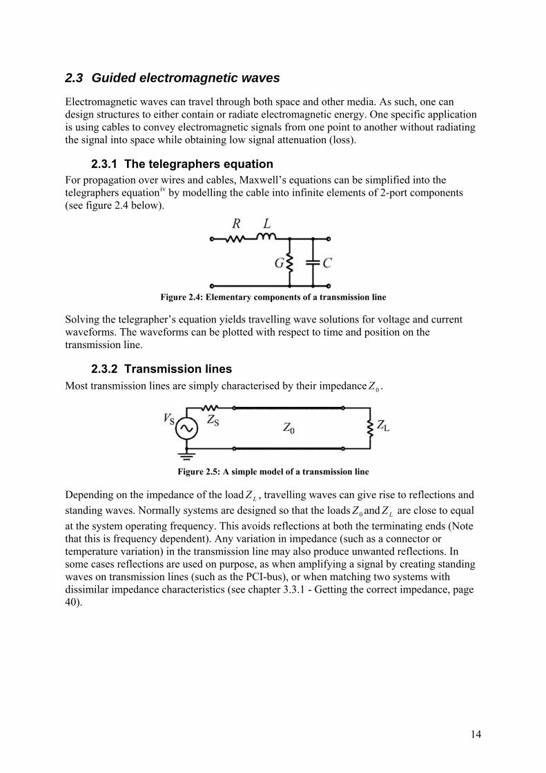
2.3.1 The telegraphers equation For propagation over wires and cables, Maxwell’s equations can be simplified into the telegraphers equationiv by modelling the cable into infinite elements of 2-port components (see figure 2.4 below).
Figure 2.4: Elementary components of a transmission line
Solving the telegrapher’s equation yields travelling wave solutions for voltage and current waveforms. The waveforms can be plotted with respect to time and position on the transmission line.
2.3.2 Transmission lines Most transmission lines are simply characterised by their impedance 0Z .
Figure 2.5: A simple model of a transmission line
Depending on the impedance of the load LZ , travelling waves can give rise to reflections and
standing waves. Normally systems are designed so that the loads 0Z and LZ are close to equal
at the system operating frequency. This avoids reflections at both the terminating ends (Note that this is frequency dependent). Any variation in impedance (such as a connector or temperature variation) in the transmission line may also produce unwanted reflections. In some cases reflections are used on purpose, as when amplifying a signal by creating standing waves on transmission lines (such as the PCI-bus), or when matching two systems with dissimilar impedance characteristics (see chapter 3.3.1 - Getting the correct impedance, page 40).

15
Figure 2.6: Looking at the transmission line with respect to voltage, time and placement x.
For low frequencies, or DC-current, transmission line characteristics are not a concern. The reason for this is because the electrical lines, most often, are very short in relation to the wavelength of the signals they carry. For instance, the wavelength of a 50Hz AC power-line is
f
ec km
Hz
skm6000
50
1/300000
[Eq. 2.1]
e represents the velocity-factor of the transmission line.
c represents the speed of light.
f is the measured frequency.
Considering the setup in Figure 2.6 above, and assuming a no-reflection scenario, the voltage between A and 'A at point 0x , when driving the source, would be given from the formula:
)cos(),0( 0' tVtVAA [Eq. 2.2]
The resulting voltage between B and 'B at any length x at time t is given by the formula:
)
2cos(
)cos(),0(),(
0
0''
xtV
ec
xtV
ec
xtVtxV AABB
[Eq. 2.3]

16
Evaluating the last term,
x2
[Eq. 2.4]
shows that for low frequency signals, the voltage at any point on the transmission line only varies with respect to time:
)2
cos(),( 0' x
tVtxVBB
)cos(0 tV [Eq. 2.5]
2.3.3 E and H-fields for transmission lines Transmission lines are, as stated earlier, constructed so that the electromagnetic-waves they conduct are not radiating into space. To achieve this, a general understanding of how the fields behave is a must.
In order to construct a decent antenna cable, there are only two main concepts that will produce a product capable of transferring high-frequency signals without too much cable loss; the two wire construct, and the coaxial cable.
The two-wire transmission line has the advantage that the direction of current flow in one conductor is always opposite to the other, so the fields strengthen one other between the conductors but cancel each other out away from the conductor. In order for this type of cable to maintain constant impedance, a constant distance between the conductors has to be maintained. Also, no metallic conductors should be in direct vicinity of the transmission line as this will interfere with both the E-field and the H-field.

17
Figure 2.7: The construction (a), visualization of the E-field (b) and the magnetic field (c) in a two-wire
setup.
Due to the nature of electromagnetics, a signal in this type of cable has a velocity factor e close to 0.95. This means that a signal in this type of cable moves with a speed at 95% of the speed of light c .
The fact that this type of cable is influenced by nearby metallic objects makes it hard to use with any advanced system components like cable rails, gutter pipes and rigs as they are mostly made of metal.
The coaxial design makes such a cable much less sensitive to nearby metallic (or generally conductive) objects mostly due to the fact that the E-field is contained within the cable itself.
Figure 2.8: Visualization of the E-field (a) and the magnetic field (b) in a coaxial design.
The coaxial outer conductor is normally attached to ground. Because of this, the centre conductor is often looked on as a single signal carrier.
The coaxial transmission line typically has a velocity factor of 0.66.

18
2.3.4 Reflections From Eq. 2.3 above, one can plot the voltage across the cable at any specific time interval. However, this does not account for reflections when the cable-end impedance of are not the same as the impedance of the cable itself.
If a signal is travelling along a transmission line with a set value of impedance and then meets another part of the transmission line with different impedance, parts of the signal is transmitted onwards, while the rest is reflected. Depending on whether the transmission was from a high to a low impedance, or opposite, the reflection has either a 180º (π) or a 0º degree phase-shift (see figure 2.9 and figure 2.10 below).
Figure 2.9: The signal reflection gains a 180° phase shift when going from relatively high impedance to
lower impedance.
Figure 2.10: The signal reflection has no phase shift when going from relatively low impedance to higher
impedance. The size of the reflection is, of course, zero, when there is no difference of impedance. When there is a reflection, one can calculate the reflection coefficient using the complex ratio of the electric field strength of the reflected wave (E −) to that of the incident wave (E +). The ratio describes how much of an incoming signal would be reflected back when the signal is transmitted between the two devices or mediums.
E
E [Eq. 2.6]
Notice that a negative reflection coefficient corresponds to a phase shift of 180° (or π) of the reflected wave. The ratio is +1 when there is a complete positive reflection (open circuit). The ratio is -1 when there is a complete negative reflection (short circuited).
The reflection coefficient may be established using other types of field or circuit parameters, one of them being the characteristic impedance of the source and load impedance measured individually.
SL
SL
ZZ
ZZ
[Eq. 2.7]
From eq. 2.7 one can easily postulate that when 0 SL ZZ , the return loss is 0. If the
source SZ has lower impedance than the load LZ , a large percentage of the signal is reflected.
Phase-shift: π or 180°
High impedance, ZS Low impedance, ZL
Phase-shift: 0
High impedance, ZL Low impedance, ZS

19
Another way of looking at the reflection coefficient is by the voltage standing wave ratio, or VSWR. When a signal is reflected, standing waves are formed on the incident cable. At some points of the cable the incident and reflected wave will interfere constructively, while destructive at other. Measuring the minimum and maximum absolute voltage along the cable, or at different frequencies, the voltage standing wave ratio can be found for any device.
min
max
1
1
V
VVSWR
[Eq. 2.8]
Only the magnitude is of interest when finding the VSWR.
2.4 Antennas
There are many types of antennas, where most of them are designed to achieve specific tasks. Some are made so that they can work over a wide spectrum of frequencies (broadband), others supporting only a narrow bandwidth. Antennas can be specialized to fit certain size limitations, cost limitations or durability demands.
Other antennas, normally the slightly bigger ones for stationary mounting, have a high directional gain enabling it to receive weak signals from far off places. This is the type of antenna we need to be able to communicate with a small satellite with limited transmit power. In order to explain how such an antenna works, one must first start with the simples of antennas.
It is assumed that antennas are passive reciprocal devices. By this one can assume that they will have the same gain when used either for transmission or for reception of electromagnetic energy.
2.4.1 The isotropic radiator Behind any successful antenna design, the theory behind travelling waves must be taken into consideration, and to measure its capabilities the antenna may be referenced to the most rudimentary antenna that can be though of; the theoretical (conductive) single point in space called the isotropic radiator:
Figure 2.11: The theoretical isotropic radiator
The intensity of radiated power normally equals the cross product of HE , however, for an isotropic radiator, the radiation pattern
),(ˆ4
),,(
ur
erE
jkr
[Eq. 2.9]
would violate the Helmholtz wave equationv, a derivative of Maxwell's Equations.
But still, the theoretical radiation pattern from [Eq. 2.9] would yield a completely round (spherical/isotropic) radiation pattern at any and all frequencies.
Diameter d = 0 The isotropic radiator

20
The isotropic radiator depicted above would never work as the “perfect antenna” (even with 0d ); because a coherent isotropic radiator cannot exist for the same reasons that a magnetic monopole cannot exist.
Still, the theoretical radiation pattern that the isotropic radiator represents is a de facto standard for comparing antenna gain in dB. When referencing any antenna-gain compared to an isotropic radiation pattern, the term dBi is used.
The smallest directivity a radiator can have relative to an isotropic radiator, is a Hertzian dipole (a small dipole relative to the wavelength), which has a directive gain of 1.76 dBi.vi
2.4.2 The dipole Let’s consider a radio with a short ended antenna output:
Figure 2.12: Radio with short ended output
Assuming that the antenna-cable has the same characteristic impedance as the transceiver output and that the cable ends in an area of infinite impedance, eq. 2.7 on page 18 provides the reflection coefficient occurring at the cable end:
SL
S
SL
L
SL
SL
ZZ
Z
ZZ
Z
ZZ
ZZ
SL
S
SL
L
Z ZZ
Z
ZZ
ZL
lim
1
01S
S
S Z
Z
Z [Eq. 2.10]
A reflection coefficient of 1 basically means that 100% of the signals transmitted from the transceiver are reflected back at the cable end. As a consequence, standing waves are formed in the cable, and as there can be no current at the end-point (meaning the impedance is infinite), the energy must be dispersed elsewhere. With a radio having, as an example, 50 watts of maximum output power, then nearly all of this energy must be dispersed in either the radio or the cable itself (as nothing comes out the end). Assuming the cable has a low loss at the selected frequency, most of the 50 watt of energy is deposited in the radio equipment. This leads to local heating that may prove devastating to any electronic equipment and should therefore be avoided.
Of course, neither vacuum nor air sports infinite impedance, so this may not be completely true, but even so, we now know that a radio should never transmit while unconnected. If no antenna is available, the cable may be terminated by a simple resistor. To achieve a reflection of zero, the resistance should match the impedance of the cable and radio.
Radio Tranceiver

21
Figure 2.13: A radio with a short ended output, forming standing waves. Because the distance between the conductors is none-zero, some electric and magnetic fields does radiate from the cable end, but these fields
tend to cancel each other out as they move away from the cable end.
To achieve the opposite of a (near) total reflection, solving eq. 2.7 on page 18, for zero reflection, or 0 , gives:
SL
SL
ZZ
ZZ
when,0 LS ZZ [Eq. 2.11]
So, a radio system must therefore provide matched characteristic impedances at radio output, transmission line and antenna in order to maximize throughput.
Considering figure 2.13 above, the setup looks very much like a very short dipole antenna (a.k.a. a Hertzian dipole), where the two line ends are turned at right angles. With the cable ends turned outwards, the electrical field-lines are forced away from the cable, thereby radiating an E-field. As the voltage between the tips of the dipole increase, the current that flows between the ends generates a magnetic field. The magnetic fields arising from the two conductors now has the same rotational aspects and thereby amplifies one another, when in the far field, instead of cancelling each other out as they did while in the transmission line.

22
Figure 2.14: Making a dipole antenna from two angled wires
From a distance, the relative length, and thus the phase difference, to each antenna element will only vary with the angle of approach and not the distance to the antenna itself. Looking away from any local field the antenna may be generating helps keeping the formulas simple. This is called the far-field approximation, and is what is normally assumed when talking about antennas. The far-field is defined as when we consider the electromagnetic fields approximately 10 , or more, away from the source.
The electrical field arising from figure 2.14 can be described by the setup:
)(
0
0
4
sin krtieL
cr
iIE
[Eq. 2.12]
E is the far field of the electromagnetic wave radiated in the direction
0 is the permittivity of vacuum
c is the speed of light r is the distance from the doublet to the point where the electrical field E is evaluated
k is the wave number 2
k
0I is assumed to have a intensity as shown on the picture
L

23
Figure 2.15: Current distribution on a short dipole
As the voltage shifts polarity according to the frequency of the signal, an EM-wave (radio-wave) similar to the modelled light beam in figure 2.3, chapter 2.2 Electromagnetic waves, is made. The electric and magnetic fields are perpendicular to both each other and the direction of propagation.
The resulting emission diagram equals a torus, with the short dipole placed in the centre.
Figure 2.16: Emission diagram of a short dipole takes the form of a torus
Knowing the electric field, one can calculate the radiated power and the resistive part of the series impedance of the dipole. This is known as the radiation resistance:
2
06
LZRSeries , for L . [Eq. 2.13]
Where 0Z is the characteristic impedance of free space.

24
Using the approximation of 1200 Z gives:
ohmL
RSeries
2220
[Eq. 2.14]
Narrowing down the antenna design to a specific frequency we can now solve for what length a dipole must have to have a resistance of 50 Ohm at any specified wavelength. Selecting a frequency of 150MHz ( =2m) shows that:
20SeriesR
L
meter0.150.05.220
50
[Eq. 2.15]
However, although this is pretty close to a real 50 Ohm dipole, the requirement of L has been breached. We have to account for the speed of which the transverse waves on the dipole are travelling. Assuming a speed of 95% the speed of light, any frequency f will have a
wavelength fce where e represents the relative speed of the electrical field-variations versus the speed of light in vacuumc . The antenna should therefore end up being 5% shorter than in Eq. 2.15 above:
meterf
ceL 95.0
250.0
[Eq. 2.16]
Also, we have not taken into account the imaginary part of the characteristic impedance that will gain a significant size when the length of L is approaching . Even so, we can now safely assume that a dipole with a length 2L makes a pretty good antenna, but this needs further investigation.

25
Revising the layout of figure 2.14 above, turning each electrical quarter wavelength ( 4 ) ends of the conductors at a right angle, increases the radiation of electromagnetic waves by matching the antenna impedance to the transmission line, and the free space surrounding it.
Figure 2.17: Construction of a half-wave dipole antenna from two angled wires
Knowing that the signal is reflected back (without phase shift) at each end of the quarter wavelength stubs, a plot of the maximum occurring voltage across the 2 dipole is possible. Assuming a sinusoidal distribution gives:
Figure 2.18vii: Maximum voltage across a dipole
Noting that the two quarter wavelength stubs has opposite voltage, and that the voltage on each end is doubled due to the reflection in the 4 stub, provides a higher differential voltage than what would have been with other lengths. This can only be looked upon as a bonus!
Figure 2.19: Maximum current across a dipole
26
With the revision of the dipole length, inserting 2L and revising the formula in Eq. 2.12 on page 22:
)(
0
0
0
0
sin
cos2
cos
24
sin krtikrti ecr
iIe
L
cr
iIE
[Eq. 2.17]
One should notice that the fraction
sin
cos2
cos
is pretty much the same as sin .
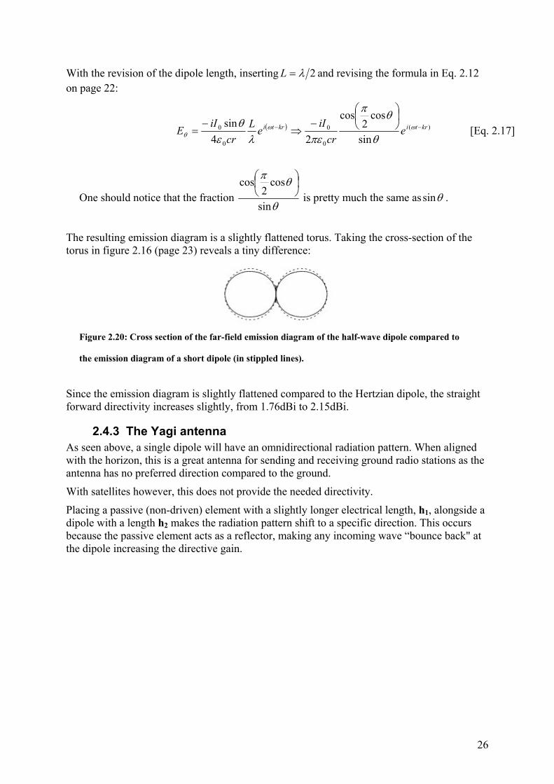
The resulting emission diagram is a slightly flattened torus. Taking the cross-section of the torus in figure 2.16 (page 23) reveals a tiny difference:
Figure 2.20: Cross section of the far-field emission diagram of the half-wave dipole compared to
the emission diagram of a short dipole (in stippled lines).
Since the emission diagram is slightly flattened compared to the Hertzian dipole, the straight forward directivity increases slightly, from 1.76dBi to 2.15dBi.
2.4.3 The Yagi antenna As seen above, a single dipole will have an omnidirectional radiation pattern. When aligned with the horizon, this is a great antenna for sending and receiving ground radio stations as the antenna has no preferred direction compared to the ground.
With satellites however, this does not provide the needed directivity.
Placing a passive (non-driven) element with a slightly longer electrical length, h1, alongside a dipole with a length h2 makes the radiation pattern shift to a specific direction. This occurs because the passive element acts as a reflector, making any incoming wave “bounce back" at the dipole increasing the directive gain.

27
Figure 2.21: Simple Yagi setup
A cross section of the far-field emission diagram of a Yagi shows that the antenna is more sensitive in one direction than the other:
Figure 2.22: Cross section of a 2-element reflector-Yagi emission diagram depicting the main and back
lobe.
In order to maximise the directive gain, the distance from the reflector to the driven element should be placed around 2.0 away from the reflector, as seen in figure 2.23 below.

28
Figure 2.23viii: Gain in dB of a 2-element Yagi relative to a single dipole when varying element spacing
By definition, a Yagi-antenna only consists of two elements where one is the driven element (the dipole). The other element can either be a reflector as seen above, or a director. The size of the director must be slightly smaller than the dipole and as seen in figure 2.24 below, the emission diagram is exactly similar to the reflector design, only that the maximum gain direction is reversed.
Figure 2.24: Cross section of a 2-element director-Yagi emission diagram depicting the main and back
lobe.

29
2.4.4 The Yagi-Uda array Combining the reflector and director from the two types of Yagi-antennas, a so called Yagi-Uda array can be made. Also, the number of directors in the design could be increased to further increase the directivity of the design.
Figure 2.25: A Yagi-Uda array consists of a reflector (1) the dipole (2) and a number of directors (3...k)

30
2.4.5 The cross-Yagi The cross-Yagi basically consists of two interleaved Yagi-Uda arrays, with each of the arrays perpendicular to the other. Using this setup, while ensuring a proper phase-delay between the two arrays, a circular polarization can be achieved.
Single dipole antennas would produce an electro-magnetic signal similar to the light beam depicted in figure 2.3 on page 13 where both the E-field and H-field would keep a constant orientation to any given plane along the travelling direction. If the dipole is oriented perpendicular to the ground, the antenna would transmit and receive signals were the E-filed would be varying in a vertical manner.
Tilting the antenna 90° along the direction of transmission, any transmission would have the E- and H-field perpendicular to the fields in the previous setup. The two antennas would therefore not be compatible.
Figure 2.26: Showing the variation of the E-field using vertical (1) and horizontal (2) polarization
Figure 2.27: Showing the variation of the E-field when receiving a Left Hand Circular Polarization
(LHCP) and Right Hand Circular Polarization (RHCP)
1 2
1 2

31

32

33
3 Construction of the Oslo Ground Station – Part 1
In the recent years, universities around the world have begun applying small size LEO8-satellites for various scientific and engineering applications. LEO-satellites have an orbit far closer to the earth than for example GEO9-satellites. LEO-satellites have an orbital time in the 1-2 hour area, resulting in relatively short clear-sight windows of communication between a satellite and a geographically fixed earth station. Normally a satellite pass takes a minimum of 3 minutes to a maximum of 9 minutes. Even though a LEO-satellite is far closer to earth than a GEO-satellite, the small size and limited power available on a Cube Sat10 or similar sized space born boxes will inexorably make the signal, or EIRP11, from the satellite relatively weak. One of the major issues in LEO-satellite communication is the problems that arise when using narrow beam directive antennas. Since the satellites do not have a fixed location relative to ground as in GEO-satellites, any use of directive antennas much include a way of pointing it in the correct direction at the correct time. Since such a system is difficult to include on a small size satellite, the answer is to use a high gain directive antenna on the ground. This calls for a ground station system that is able to steer an antenna rig in the correct direction at the correct time, and track the satellite as it traverses across the sky. In addition, the system must also account for the varying received frequency from the effects of Doppler-shift that occurs due to the high relative speed of the satellite.
3.1 General principles
There are many ways of designing a satellite ground station; however, there are some system parameters we in this case aim for:
a) The system is to communicate on amateur-radio frequencies12, mainly in the 2m and 70cm-band13.
b) Follow the present laws and regulations regarding this.
c) Achieve a high reception gain reducing the need of a high powered transmitter on the satellite.
d) Ability to modulate and demodulate a digital signal.
e) Remote operation.
Part d) and e) will be covered in chapter 5 - Construction of the Oslo Ground Station – Remote operation. 8 Low earth orbit; an orbit with an altitude of approx. 100km to 900km and a corresponding orbital time of roughly 1-2 hours. Very often the satellite is placed in a highly inclined orbit so that the satellite “scans” the entire surface of the earth during a 12 or 24 hour period. 9 Geostationary earth orbit, an orbit with an altitude of approx. 42 357km, and an orbital time of exactly 24 hours, and therefore has a fixed sub-satellite point, meaning that the satellite is stationary from a surface of the earth point of view. 10 A Cube Sat is a type of space research pico-satellite with a dimension of 10×10×10 centimeters, alternately with a combined size of up to three of these cubes in a row. 11 Effective Isotropic Radiated Power 12 The International Telecommunication Union (ITU) governs the allocation of satellite communications frequencies worldwide. However, most Cube-sats use the amateur frequencies that can only be used by licensed users for non-profit, non-commercial use. 13 The radio-band name comes from the approximate wavelength of the frequencies they represent. 2m-band represent the amateur frequency-band of 144.00-148MHz. 70cm-band is at 430-450MHz.
34
A high gain antenna inexorably has a narrow beam-width (or main lobe), and we therefore need to keep the antenna pointed towards the satellite throughout the pass. This leads to a new sub-goal:
f) Ability to aim the antenna rig in the correct position at the correct time, and track the satellite as is traverses the sky.
A LEO8-satellite has a relatively high speed compared to a fixed point on the earth, so as it enters the horizon, any radio-content will be received at a higher Doppler-shifted frequency than what the satellite is transmitting at. Also, radio-signals transmitted from the ground will not be received at the satellite at any fixed frequency unless the frequency-shift is correct at the ground. To account for this the system should also aim at:
g) Correct for the Doppler-shift by continuously setting the correct receiving and/or transmitting frequency.
The systems effectiveness will mainly be defined by the number of antennas. In the initial setup, we will be using a single cross-Yagi antenna for each frequency-band (2m and 70cm)14. If this, at a later time, proves inadequate, we have the possibility of adding more antennas. We selected a couple of antennas15 from Tonna, as they were cheap and had a relatively high gain. Also, they are stackable if we later want to improve the link-budget.
We also have to use rotors to keep the antenna pointed towards the satellite as it moves across the sky. For this we have selected the frequently used Yaesu G-5500 dual rotor system, with a Yaesu GS-232B computer control interface. The control interface is normally connected to a computer with an RS-232 serial-cable.
Selecting the ICOM 910h for radio operation, the simplest form of interface between a computer and the radio would be a level converter called CT-17 that interfaces, or more accurately level converts, the radio’s CI-V bus to a standard RS-232 serial cable (and backwards). In the Oslo Ground Station, this is achieved through a custom made level-conversion on the PCB.
If you are to automatically control the radio, the simplest way to achieve this would be to use the standard ‘remote desktop connection’ to the computer connected to the radio and rotor controller. However, sharing passwords and adding users on a computer is not acceptable when the computer if part of a large “corporate” network like the university network.
The way to get around this was to design a ground station controller and terminal node controller, or TNC, as a single separate unit.
14 The band name comes from the approx. wavelength of the frequencies they represent. 2m-band represent the amateur frequency band of 144.00-148MHz. 70cm-band is at 430-450MHz. 15 Tonna 20818 2m 2x9element. cross-yagi and Tonna 20438 70cm 2x19element cross-yagi

35
3.2 Deciding on rigging materials
3.2.1 Rig mounts Long before the project began, two antenna-towers had been erected on the roof of the physics building16. Luckily none of them contained any antennas in use, so selecting a site for the antenna-rig would not be a problem. The rig closest to the room available for radio operation would be the northernmost, so this was selected. With this rig, the most practical place to attach the azimuth-rotor would be “inside” the rig, at the bottom of the main pole (see figure 3.1 below). This setup, compared to placing the rotors together at the top makes the rig more stable in windy conditions and will presumably be less prone to failures as wind and wind stress on the azimuth rotor is minimized. For this to work, a so called separation-kit was purchased. This mainly consisted of screw and clamps so that the elevator could be attached to a vertical pole.
16 The Physics building is one of the oldest buildings at the University of Oslo, with a visiting address of Sæm Sælandsvei 24. Oslo, Norway. Antenna altitude: (approx.) 95m above sea level. Coordinates: 59.93814ºE, 10.71800ºN

36
Figure 3.1: The antenna tower (1) with the main vertical pole (2), the cross-bar (3), the azimuth rotor (4), the elevator (5) and the low noise amplifiers (LNAs) (6).
The main vertical pole (2) must be sturdy and support a lot of weight, so using anything out of metal for this seems the most logical choice. On top of this pole, the elevator is fixed to the vertical pole using two metal clamps and fitting screws. This is called a separation kit, and had to be purchased after we discovered that this was not standard supplied accessory. A horizontal cross-bar (3) is feed through the elevator, with the antennas mounted at each end. Yaesu specifies that this bar should have a diameter between 38 and 41mm. However, they do not specify the material best suited for the task, only that a none-conductive material will give better performance (signal-wise) than a conductive material. The two choices were aluminium and PVC-tubing, and were a hot topic of discussion where the pros and considerable both in number and weight:
- Aluminium conducts electricity, and would affect the E-field, causing a degradation of signal reception. However, this effect is effectively halved due to the circular polarization setup used.
+ PVC is none-conductive and should not afflict the E-field as much, and therefore provide the best possible reception.
- Any horizontal piece of PVC may ‘sag’ and cause the antennas at either end to loose their position relative to each other. This will negatively influence the signal gain.
- PVC may not provide enough hold to the antenna bracket attachment, and might cause the antennas to “tilt” during windy, snowy or icy conditions.
- If we later would want to add more antennas to the rig (called stacking), a PVC-tubing would prove insufficient for the extra load of more antennas, and would have to be replaced either way.
5
2
1
4
3 6

37
In the end a solid aluminium crossbar was selected even though the signal might get slightly attenuated. This decision was based on the assumption that a PVC-solution would cause problems during the construction, or later, as the PVC is not nearly as sturdy as aluminium.
3.2.2 Cabling There are essentially two kinds of coaxial cable design; the coaxial with a solid core (centre-lead), and one with a threaded centre-lead. The one with a solid copper core normally has an air-filled separation between the centre and outer conductor17. This normally results in a lesser loss than in a threaded centre-lead cable18. However, a threaded cable does have a much better ability of flexing than the single core. In fact, a single core cable should never be used to interconnect a moving rig. From the radio to the pre-amplifiers on the rig, approx. 2x60m of Westflex103 (solid core) are used. From the pre-amplifiers to the lightning arrestors and from there to the impedance adaptor (the splitter), RG-213 (threaded core) is used. This cable is also used from the impedance adaptor to the dipoles on the VHF-antenna. The splitters use 75 Ohm RG-11 cables (solid core) to implement the impedance adaptation. The fact that RG-11 is solid-core is no problem, as the stretches are so short.
3.2.3 Low noise amplifiers Low noise amplifiers, or LNA’s, are an important part of designing a high quality rig for receiving weak signals. This amplifier is put as close as possible to the antenna, so that cable loss is minimised. Most radio amateurs agree that one should never buy an expensive radio, without first buying the absolute best LNA available. The reason for such bold talk is rather simple. No matter how much power you put out while transmitting; there will be no conversation unless you can hear the other party while receiving.
In fact, with a high powered transmitter, you even may risk interrupting other people’s conversations without knowing. Also, when receiving a weak signal, the worst thing you can do is to make the signal pass through longer lengths of cable to the radio unamplified. From the moment the signal enters the antenna it is influenced not only by cable loss, but also picks up thermal noise (see chap. 4.1.8 - System noise temperature). To minimize this effect, it is important to amplify the signal as fast as possible to prevent excess signal degradation. Also, this amplification should most importantly introduce as little system noise as possible.
By their specifications alone (see appendix B) and by customer reviews19, the SP-2000 and SP-7000 by SSB-electronics (sold under the name Microset) are considered the best on the market.
17 Our main cable, Westflex 103, has a solid copper core and air-filled separation, and has are spec’d with a total loss of 7.5dB/100m @ 432MHz, or 4.5dB/100m @ 144MHz 18 Our secondary cable, RG-213/U, has a threaded (7 threads) copper core and plastic-filled separation, and has an approx. total loss of 15dB/100m @ 432MHz when using a system with an SWR of 1:1. A loss of 8.5dB/100m @ 144MHz 19 http://www.eham.net/reviews/detail/4156, last visited 18/02/10

38
3.3 Building the antennas
The two antennas, the Tonna 20818(2m 2x9 el.) and 20438(70cm 2x19 el.), arrived in a ‘build it yourself’-set and had to be accurately assembled, mounted, cabled and tested. Even load-matching had to be done manually by cutting and soldering exact lengths of cables with different impedance, see chap. 3.3.1 - Getting the correct impedance.
The first thing we had to do was to attach all the directors and reflectors to the antennas, as described in the manuals that came along. This was one of the simplest things to do, as it was fairly straight forward work. However, thinking that this would be a breeze would prove to be a wrong. As work progressed, outcries like “we’ve mounted everything the wrong way” or “the manual does not say anything about this” were commonplace. Many things had to be redone several times, as people mounted everything the wrong way, or were confused by the holes in the ends of the main bar or the extra holes put in for cable guidance. In addition, the plastic clamps fixing the dipoles had been overheated at some point (probably during production), so that they did not fit. The clamps had to be “reshaped” using a soldering iron. It appears that spending some extra cash on antennas might save you some time during system setup after all. However, for students working “for free”, this is not a problem.
Having built the antennas, and connecting the antennas front piece and a rear piece together, we could clearly see that one of the antennas (the VHF) buckled in the middle due to a weak attachment of the two end pieces.
The front and rear piece were, from the manufacturer, meant to be latched together at the middle using a metal piece that attaches the antenna to the rest of the rig (via the cross bar). Because this obviously would result in a weak connection, we drilled two holes in the main bar, and let the instrument-tool shop20 lend a hand in making a fitting aluminium piece to strengthen the joint (see figure 3.2 through figure 3.4 below).
20 Instrumentverkstedet, located at the Institute of Physics, Oslo. See also(in Norwegian): http://www.fys.uio.no/omfi/enhetene/verksted/

39
Figure 3.2: Bottom- side picture of the top attachment piece (1), the rear end of the front antenna boom
(2) and the custom made aluminium piece with screw-holes (3).
Figure 3.3: Inserting the custom aluminium piece
Figure 3.4: Depicting the top attachment piece (1) with inserted screws, the lover attachment piece (2), the rear end of the front antenna boom (3), the front end of the rear antenna boom (4) and the rig supporting
cross-bar (5).
1 2
3
13
2
4
5

40
3.3.1 Getting the correct impedance Considering antenna cables, one must remember to use cables with the same impedance as the equipment connected at either end. Today, two types of VHF and UHF antenna-systems are used; 75 Ohm for regular TVs, and 50 Ohm for basically everything else.
A cable with a diameter of 10 mm and impedance of 77 Ohm would provide the smallest possible cable-loss when using air filled coaxial( 1r ). In this technology, the space between the core and the shield is mostly filled with air, using plastic, or PTFE, as spacers. With a solid copper core, any such cable is considered high quality. The WestFlex103 used for the longer stretches in the Oslo ground-station, although with a 50 Ohm impedance, is made this way. Cheaper cables use solid PTFE ( 2.2r ) or PTFE-foam ( 43.1r ) as spacers, and threaded metal core.
Figure 3.5ix: Cable loss versus impedance, in a copper coax with a 10mm diameter.
Although an air filled copper coax at 77 Ohm provides the lowest loss, this impedance is not optimal when considering the maximum break-down voltage, so this is only suitable in a receive-only system (like TV-sets). Coincidently, TV’s normally don’t normally use air-filled spacers, as they are expensive to make. Often a solid- or foam-PTFE is used instead. So why isn’t 50 Ohm cables used in TV-systems to provide the lowest loss? The reason, again, is price. Increasing the impedance slightly decreases the diameter of the metallic centre-core. This makes TV-cable cheaper. In addition the cable becomes more flexible and user friendly.
When considering transmit/receive systems, there is another characteristic that needs to be considered. When trying to push large amounts of power through an air-filled coax cable, a 50 Ohm cable would have the highest break down voltage (see figure 3.6 below). A 30 Ohm cable would provide the maximum voltage/current trade-off (supporting the maximum power). The maximum voltage available will depend on several factors like humidity, air pressure (high above the sea), temperature and surface roughness of the copper core. In figure 3.6 below, a break-down voltage of 100 kV is assumed. A simple way to increase this would be to fill the air-gap with solid PTFE, or other plastics, but then the cable loss would be increased. A solid PTFE coax normally can handle up to 10 times the power than air-filled coax. Often the power-limitation can be lifted up to at least 10 kW using solid PTFE.

41
Figure 3.6: Maximum power and voltage handling of a 10 mm air filled coax (internal voltage break-down
at 100 000 V/m)
Most amateur-radios today use a 50ohm setup. This is also true for the ICOM 910h used in the Oslo ground-station, so we must use 50 Ohm cables for this system.
Basically, if you have a transceiver designed for 50 Ohm operation, one would also use antennas with 50 Ohm impedance characteristic. But this is not always possible as two 50ohm antennas in parallel would yield a total impedance of 25 Ohm which would give an impedance mismatch between the radio and the antennas. Adding more antennas would of course make this mismatch even worse.
In case of a mismatch, an “impedance-matching-setup” has to be made. For small frequency-bands this can be achieved by introducing a matching-stub (piece of cable) into the system. This has to be done when connecting multiple antennas together (for example would two 50ohm antennas in parallel gives a total impedance of 25 Ohm, which would give an impedance mismatch).
As explained in chapter 2.4.5-

42
The cross-Yagi, a cross-Yagi is made up of two Yagi-Uda antennas intertwined in a perpendicular manner. As consumers normally would like the possibility to send or receive both linear (mostly ground based communication) and polarized signals (mostly satellite communication), each of the intertwined antennas is made to conform to the industry standard 50 Ohm impedance. This is all and well if you are only to use one of the antennas at a time, but when operating with polarized signals, the two antennas have to be connected together in a parallel manner. But as explained earlier, two equal loads in parallel will in total yield a load half of their own. In essence, the two 50 Ohm antennas would yield a load of 25 Ohm. This does not match the radio or cable-system well, so two so called matching stubs has to be made.
A quarter-wave cable can act as an “impedance adapter” between two known, but unequal impedances, 1Z and 2Z . Notice that this only works within a narrow bandwidth, as any other frequency imposed on the system than the one designed for, would not see the matching stub as a quarter-wave. The matching stub should have intermediary impedance Z according to the quarter wave formula:
21 ZZZ [Eq. 3.1]
If both the two antennas in question would have a virtual 100 Ohm termination, the parallel of these would total in a fitting 50 Ohm. Using a 50 ohm antenna as a starting point, creating a theoretical 100 Ohm termination point, you would need a quarter-wave (lengthwise) cable with the impedance of:
OhmZ 71.70500050100 [Eq. 3.2]
Of course, a cable with impedance of 70.71 Ohm is not readily available, but a standard 75 Ohm cable should suffice. Since the lengths of these are relatively short, the loss/meter is not important. A few meters of the cable type RG-11 was found in-house. The electrical group velocity e of this cable is the pretty standard 0.66 times the speed of light.
To connect the vertical and horizontal antennas to the radio, we basically used the setup shown in figure 3.7 below.
Figure 3.7x: Impedance matching of a 1:2 split

43
Note that the two 75ohm-cable has a length of a quarter wavelength. The electrical wavelength is shorter in a coaxial cable than in vacuum, since the signal speed in a coaxial cable normally is 0.66 times the speed of light (in vacuum).
As we are constructing two antenna-arrays for two different frequencies, two sets of matching stubs should be made with the electrical quarter length from the formula:
4
1
4
f
ce
e vacuumwavequarterelectrical
[Eq. 3.3]
Radio band length 2m 70cmFrequency 145 430 MHz
Wavelength (vaccum) 2,069 0,6977 meterRelative electrical group velocity 0,660 0,660Electrical wavelength (coax) 1,366 0,4605 meter
Electrical quarter-wavelength (coax) 34,14 11,51 centimeter
Table 3.1: Quarter wave-length calculations
In addition, one must consider the type of polarization the antenna is to be tuned to. This is done by setting a phase-delay between the horizontal and vertical antennas on the crossed yagis (see figure 3.10 below). The physics behind this is described in chap 2.4.5 -

44
The cross-Yagi.
Trying the best I could, the two impedance-splits ended up looking similar to the illustration in figure 3.7:
Figure 3.8: Two impedance-splits (1) going from RG-213 cable (2) to pairs of RG-11 cables with quarter-
wave lengths. The second split has been covered with self-sealing tape and is ready for outdoor use.
3.3.2 Selecting a polarization There are basically 2 ways of polarizing electro-magnetic waves; linear and circular. Linear polarization means that the E-field is varying in a specific angle. Practically, one normally keeps to either a vertical or horizontal polarization. On ground to ground radio systems it is fairly easy to keep track of what is vertical and horizontal, as any antenna positioned perpendicular to the ground will transmit and receive using vertically polarized EM-waves. Having a point to point system with a vertically and horizontally polarized antenna at each site, any frequency-channel can be used twice (resulting in a doubled frequency-efficiency/Hz).
This is used in satellite-TV systems when receiving data from GEO-stationary satellites. This is possible because the satellites are stationary relative to ground. When setting up a receiving station the antenna has to be tilted some if the satellite is not located straight south.
However, when considering LEO-satellite to ground communications, keeping track of what is up and down is not as simple. As a CubeSat enters the horizon what is considered “up” will not be the same as when it exits. A solution to that would be to send and receive in a circularly polarized manner.
However, since a CubeSat is not likely to feature anything more than a dipole-antenna, nor be able to position the antenna correctly, this is not possible. The satellite would, in respect to a ground station, transmit in a non-circular manner, with a varying, possibly unknown, polarization. In order to avoid signal fading when the satellite is spinning (or just positioned the wrong way compared to the ground station) the logical choice would be to select a circularly polarized antenna on the ground station (see table 3.2 below).
Circular polarization exists of course in two forms: Right hand circular polarization (RHCP) and left hand circular polarization (LHCP).
1
3
2

45
Table 3.2: Approximate losses, in dB, arising from antenna-signal polarization mismatch
Some amateur satellites (non-CubeSat), has antennas with a defined circular polarization. Approx. 70% of these support RHCP. The ground based antennas are therefore often made to comply with this, as either LHCP or RHCP would have the same effect when communicating with a CubeSat. From table 3.2 above, we can see that this design will have an inherit 3dB signal loss when receiving a linearly polarized signal, but this is a lot more acceptable than having the signal fade in and out during a satellite pass. In the worst case scenario, were the satellite is spinning, any linearly polarized antenna would receive a fluctuating signal as the satellite moves around.
There are two ways of constructing an antenna with a circular polarization: Correctly phasing two crossed dipoles, or using helical antennas. In this thesis, phased cross-yagis are assembled for RHCP. Helical antennas tend to have a larger wind load than yagis as they require a ground plane. In addition, they do not stack as well, as the electromagnetic characteristics of a spherical antenna are not as easily defined.

46
Making an antenna consisting of two crossed dipoles, with no separation length-wise, into an RHCP or LHCP antenna is quite easy. For RHCP, following the positive maximum of the E-field, the field should have a clockwise (CW) rotation from a receiver’s standpoint. In other words, standing “behind” the transmitting antenna, the E-field must rotate counter-clockwise (CCW). For LHCP, everything is opposite. Since the dipoles are crossed at a 90° angle, the phase delay needed must be 90°.
Figure 3.9: Rear view of crossed dipoles depicting phasing-requirements of RHCP and LHCP.
Considering the two antennas in question21, each antenna has two dipoles in a crossed setup similar to figure 3.9 above, however, the dipoles are not placed right next to each other (length wise). To correct for this, the phase-delay between the two dipoles has to be specifically adapted (with corresponding reflectors and directors) do not need a simple 90° ( 4 ).
Figure 3.10x: Introducing extra phasing stubs to ensure correct polarization.
21 Tonna 20818(2m 2x9 el.) and 20438(70cm 2x19 el.)

47
Having selected RHCP, the phasing stubs must be adjusted so that the antennas will generate the proper delay in relation to the direction the signal will be travelling. Measuring the length between the vertical and horizontal dipole, keeping the measuring direction in a back to front orientation, the inherit delay between the dipoles can be calculated. As a consequence the length of the phasing stubs can be calculated. Notice that the facing stub may very well be a lot longer that calculated, as long as the other dipole is also delayed the same extra amount using the same type of 50 Ohm cable.
Also, the importance of keeping track of what is considered point 0 (in figure 3.9 above) from the time when these calculations are done to the point where the antennas are fixed to the rig and the delay cables (there’s two of them on each antenna) are attached, can not be underlined enough. In the Oslo ground station, the left tip, when the rig is in an elevation of 0° (with the elevation rotor in a 180° position, “left” would be “right”), of the rearmost dipole serves as point 0.
Setting a fixed reference-orientation of the antennas, and making sure the “positive” tips of each dipole (see figure 3.9 above) are marked properly, one can start calculating the inherit phase-delay arising from the placement of the dipoles, and then find the required length of the phasing-stub:
Antenna 2m(min) 2m(max) 70cm(min) 70cm(max)Frequency 144,00 145,99 430,00 435,00 MHz
Wavelength (vaccum) 2,083 2,055 0,6977 0,6897 meterRelative group velocity (air) 0,9997 0,9997 0,9997 0,9997Relative electrical group velocity (coax) 0,660 0,660 0,660 0,660
Wavelength (air) 2,083 2,054 0,6975 0,6894 meterDistance between dipoles (measured) 10,00 10,00 20,00 20,00 cm→Inherit phase delay 17,29 17,52 103,23 104,43 degrees
Total required phase-delay 90 90 90 90 degreesRequired phase-stub delay 72,71 72,48 -13,23 -14,43 degrees→Required length of phase-stub 0,2777 0,2730 -0,01692 -0,01825 meters
Average (in centimeters) cm27,54 -1,76 Table 3.3: Calculating the required lengths of the phase-stubs.
Notice that a phasing-stub with a calculated negative length means that the phasing stub should be inserted in front of the first dipole, instead of the second.
Due to the dual cable-guiding cylinders on the VHF-antenna, two longer stretches of 50 Ohm cable had to be used to feed the two dipoles. These two cables were made so that the one going to dipole nr 2 was roughly 27.5 cm longer than the other.

48
3.4 Patching cables
Concerning the cables used in a ground station, a fair deal of patching has to be done. The cables need to be manually terminated as each length is custom cut to every satellite rig. In most of these cases, the radio signal cables require extra attention to avoid unnecessary loss.
With the work on the Oslo Ground Station, the case with the solid core of the WestFlex103 cable is worth mentioning. The copper core (centre-lead) of this cable proved to be slightly too big to fit into the centre-piece of the cable terminators. To fit the connector tip, a set of cutting pliers had to be carefully used to lessen the maximum diameter of the core (see below).
Figure 3.11: The copper core of the WestFlex103 (1) is too wide to be inserted into the connector tip (2). It had to be made smaller by cutting alongside the centre-lead with a pair of cutting pliers (3), decreasing the
effective diameter of the centre-lead. 7
1
2
3

49
4 Satellite communication
When designing a satellite, one of the most important properties is on the ability to communicate with a ground station. Without a functioning communication link, most satellites are rendered useless. To ensure a proper satellite to ground link, one has to make estimations of the signal attenuation due to the distance to the satellite, atmospheric distortions and other system specific losses. An important aspect is noise originating in the system components and from general background radiation. This chapter with introduce the reader to the basic theory behind satellite link budgets, and propose a possible link budget for the CubeStar satellite.
4.1 Basic transmission theory
To be able to compute the power levels in a communication-link, the main aspect is the distance between a theoretical transmitter, and the corresponding receiver. The most basic transmitter would be the isotropic radiator22.
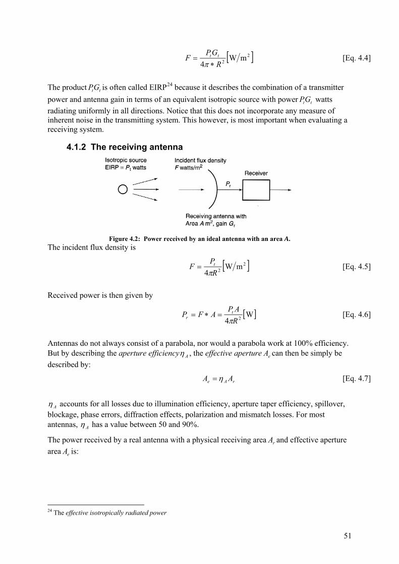
4.1.1 The transmitting antenna In free space, the transmitting source would radiate power uniformly in all directions. If a receiving antenna would encompass the entire transmitting source, 100% of the transmitted power would be transferred. This is of course absurd, but imagining that any receiving antenna is situated at the surface of a sphere centered at the transmitting source makes it easy to compare an antenna’s effectiveness by calculating its effective area. Also, this makes it possible to define the flux density at this point in space.
The surface-area of any sphere is given by the formula
24 RAsphere [Eq. 4.1]
The flux density crossing the surface of a sphere with radius R , when the source is transmitting tP watts, would then be:
22
mW4 R
PF t
[Eq. 4.2]
The effectiveness of a receiving system could then easily be described by the effective area antennaA versus the total surface area sphereA .
22 See Chapter 2.4.1 - The isotropic radiator on page 19

50
Figure 4.1: Flux density produced by an isotropic source
However, designing a satellite to ground link based on the calculated flux-density alone is not recommended, as everything from the distance between the antennas to the effectiveness of the system at different frequencies may change during operation.
Also, as described in chapter 2.4, all real antennas are always directional in the way that they radiate more power in some directions than in others. The gain of an antenna in any direction is defined as the ratio of power per unit solid angle to the average power radiated per unit solid angle.
4)(
)(0
P
PG [Eq. 4.3]
where
)(P is the power radiated per unit solid angle by the antenna.
0P is the total power radiated by the antenna.
)(G is the gain of the antenna at an angle. The term 4 converts the fractional area into steradians(abbreviated sr according to SI23)
For directed antenna systems intended for long distance communication, the direction in which the radiated power from the antenna is at its maximum is called the boresight of the antenna, and is where the angle is referenced. Most directive antennas have a given parameter of maximum gain in this direction (where 0 ). Normally, most antenna system provides a parameter for the main lobe-width. This value is twice the angle of how much an offset from can be handled before the flux density if halved (the -3dB point) compared to the boresight.
The flux density crossing the surface of a sphere with radius R , when the source is transmitting a total of tP watts with an antenna with a boresight-gain of tG would then be:
23The International System of Units (SI). The name was adopted by the 11th General Conference on Weights and Measures (1960) for the recommended practical system of units of measurement. The SI system is administered by Bureau International des Poids et Mesures. http://www.bipm.org/en/si/
51
22
mW4 R
GPF tt
[Eq. 4.4]
The product ttGP is often called EIRP24 because it describes the combination of a transmitter
power and antenna gain in terms of an equivalent isotropic source with power ttGP watts
radiating uniformly in all directions. Notice that this does not incorporate any measure of inherent noise in the transmitting system. This however, is most important when evaluating a receiving system.
4.1.2 The receiving antenna
Figure 4.2: Power received by an ideal antenna with an area A.
The incident flux density is
22
mW4 R
PF t
[Eq. 4.5]
Received power is then given by
W4 2R
APAFP t
r [Eq. 4.6]
Antennas do not always consist of a parabola, nor would a parabola work at 100% efficiency. But by describing the aperture efficiency A , the effective aperture eA can then be simply be
described by:
rAe AA [Eq. 4.7]
A accounts for all losses due to illumination efficiency, aperture taper efficiency, spillover, blockage, phase errors, diffraction effects, polarization and mismatch losses. For most antennas, A has a value between 50 and 90%.
The power received by a real antenna with a physical receiving area rA and effective aperture
area eA is:
24 The effective isotropically radiated power
52
W4 2R
AGPP ett
r [Eq. 4.8]
Worth noting is that this equation is essentially independent of frequency if tG and eA are
constant within a band. The power received at an earth station depends only on the distance R , the effective area of the receiving antenna and the EIRP of the transmitter. However, a fundamental relationship in antenna theoryxi is that the gain and the size of the antenna are related by:
2
4
e
r
AG [Eq. 4.9]
Substituting eA in eq. 4.8 with eA from eq. 4.9 above, the resulting formula provides us with an
expression of the total received power:
W)4( 2R
GGPP rtt
r [Eq. 4.10]
This equation is known as the link equation.
4.1.3 Path loss
From eq. 4.10 above, the term 2)4( R is known as the path loss, pL ; Although not a direct
loss in terms of signal absorption, this factor only accounts for the way energy spreads out as an electromagnetic wave. As such, eq. 4.10 represents an idealized case.
Noting that EIRP corresponds to the product ttGP , and recognizing pL , eq. 4.10 can be written
as:
Power receivedlossPath
gain Antenna ReceivingEIRPreceivedPower
[Eq. 4.11]
Converting all quantities into decibel, the equation can be written as:
dBWprr LGEIRPP [Eq. 4.12]
, where
dB)4(log20)4(log10
dB)4(log10
dBW)(log10EIRP
102
10
210
10
RRL
AG
GP
p
er
tt

53
In real life however, there are additional losses that needs to be considered. For a satellite to ground scenario, atmospheric losses due to attenuation by oxygen, water vapour, rain and other contaminants needs to be accounted for. In addition to attenuating the signal en route, additional losses may occur when the ground antenna is affected by changing local environments like temperature, humidity and wind. Any mispointing of the antenna may also leads to a reduction of the antenna gain.
Most of these factors are normally taken into account by introducing a system margin, but these losses have to be calculated either way to ensure an adequate estimation. Revising eq. 4.12, the result is then:
dBWrataaprr LLLLGEIRPP [Eq. 4.13]
, where
dBantenna receiving with theassociated losses
dBantenna ing transmitt with theassociated losses
dBatmosphere in then attenuatio
ra
ta
a
L
L
L
The expression dBW means decibels greater or less than 1 W, or 0 dBW. This is closely related to the more known expression dBm, which means dB greater than 1 mW. Units of dBp mean dB greater than 1 pW (picowatt).
Notice that when adding or subtracting units of dB, quantities do not have to be of the same unit, as long as the units cancels out. In eq. 4.13 all losses and gains are unit-less, while rP and EIRP are of dBW. As rP and EIRP appear at opposite side of the equal-sign, this is correct.
By keeping all satellite link parameters in dB, it is possible to enter these values into a satellite link budget. For the Oslo Ground Station, this is implemented in

54
On satellite ground stations, an LNA, or low noise amplifier, is often placed close to the antenna. In this manner, the weak incoming signal can be boosted before being transmitted down the longer coax-cable to the radio. In this way, the inherit loss in the stretch of the cable after the LNA can be ignored. While transmitting, the LNA is turned off, so that that the high powered signal can pass through unhindered. This, of course, means that one still has to consider the loss of this cable stretch while transmitting.
Figure 4.3 below shows a typical satellite to ground link overview.
Figure 4.3: A satellite link featuring an LNA, or low noise amplifier. Notice that both raL and taL often
includes eventual cable-loss from the antenna to the LNA, or from the PA, the power amplifier, to the antenna.
4.1.4 Simplified earth station
Figure 4.4: Simplified earth ground station receiver. BPF is band pass filter.

55
4.1.5 Double conversion heterodyne
Figure 4.5: Double conversion earth station receiver. The first downconversion shifts signals in a 500 MHz
band to the first 900-1400 MHz. The second downconverter has a tuneable local oscillator and channel selection filter to select the wanted radio channel/frequency in the second IF centered at 70 MHz.
4.1.6 Bandwidth, frequency deviation and other Defined by a voltage limiter at the input stage, most radios have a defined peak frequency deviation that is allowed for specific channel separation and bands. This means that if you input the maximum and minimum allowed frequency, the outputted frequencies have a specified separation.
At the same time, there is a maximum allowed frequency in the baseband content. This is also normally fixed at most radios.
Combining the two, the bandwidth of the modulated FM can be found. This is called Carson’s rule, and goes like this:
Hz )(2 maxffB pk [Eq. 4.14]
where
pkf is the peak frequency deviation of the carrier.
maxf is the highest frequency present in the modulating signal.
For analog FM broadcast, where there is a 200 kHz channel spacing, the maximum frequency deviation is set to 75 kHz. The modulating signal set to a maximum of 15 kHz. Such a radio-channel then uses:
kHz 180)1575(2 B [Eq. 4.15]

56
With the modulating signal set to a maximum of 15 kHz, this leads to a significant improvement of the signal to noise ratio, since a bandwidth of 15 kHz is effectively modulated into a bandwidth of 150 kHz.
In decibel form, the baseband NS is significantly improved:
dB 8.24148.10
15
75log20
15
180log10
log20log10
1010
max10
max10
N
C
N
C
N
S
N
C
N
S
f
f
f
B
N
C
N
S peak
This is a significant improvement over any raw NC , but this goes to the cost of uses up valuable bandwidth.
In other FM-applications, the bandwidth is significantly reduced.
Channel spacing
IF- bandwidth
Maximum frequency deviation
Maximum modulating frequency
FM-broadcast 200 kHz 75 kHz 15 kHz
The standard old voice-communication
25 kHz 15 kHz 5 kHz 5 kHz
The “new” voice-communication standard(narrow-band FM, or NBFM) (Amateur radio)
12.5 kHz 7.5 kHz 2.25 kHz 2.25 kHz
The “new” voice-communication standard(also narrow band-FM, or NBFM) (NATO)
8.33 kHz 2 kHz 2 kHz
Table 4.1xii: List of standard bandwidths
filter in the IF- FM applications use peak deviations of 75 kHz (200 kHz spacing), 5 kHz (25 kHz spacing), 2.25 kHz (12.5 kHz spacing), and 2 kHz (8.33 kHz spacing)
4.1.7 Threshold effect With an FM-demodulator, there is a certain lower level of carrier to noise ratio, or NC , where noise makes the FM signal change rapidly in phase. Because the demodulator outputs a voltage proportional to the rate of change of phase (aka. instantaneous frequency), the modulator interprets the rapid changes as frequency changes. Thus, a voltage spike will be output from the demodulator, and the signal to noise ratio, or NS , is significantly affected.

57
At higher signal to noise ratio NS is proportional to NC . The threshold is defined as when
NS drops 1 dB below this proportionality. If NC drops even further NS drops rapidly. For
most modern demodulators, this threshold is at dB 10NS xiii.
4.1.8 System noise temperature All devices, whether passive or active, generate thermal noise. For communication receivers, it is important to determine how much thermal noise is present. Comparing the noise with the signal levels is a significant part of analyzing a satellite communication link.
At higher frequencies, a black body with a physical temperature, pT , generates electrical noise
over a wide bandwidth. The power of this noise is given by:
npn BkTP [Eq. 4.16]
where
hertzin measured, ispower noise hein which tbandwidth Noise
KdegreesKelvin in source of re temperatuPhysical
dBW/K/Hz6.228101.39constant sBoltzmann' 23-
n
p
B
TK
Jk
The term pkT is a noise power spectral density, in watts per hertz. This density is constant for
all frequencies up to 300GHz. Because of this, any noise-level produced at a specific device can be compared to the noise produced by a black body radiator. If a device makes a lot of noise, one would say that its noise temperature would be high. If a device makes no noise at all, the noise temperature would correspond to zero degrees Kelvin.
When modelling noise in a system, all noisy components can be replaced with a noise-less component of the same type, but with a noise generator in front.
Figure 4.6: Noise model of a receiver.

58
When working with satellite communications systems we are always working with weak signals, so to improve the NC ratio a low systemic noise would be beneficial. By looking at figure 4.6 above, and assuming that the gain of all of the squared components in the chart is larger than 1, one can see that the only thermal noise that is amplified by all consecutive blocks is the noise from the antenna, inT , and the noise from the RF-amplifier, RFT . Assuming
that you can not decrease the noise from the antenna, the main noise-contribution would come from the RF-amplifier. This noise is then normally amplified by a couple of decades (~20dB) on a good amplifier. Because this part is so important, this is called an LNA, or low noise amplifier.
Instead of providing a noise temperature, most active radio-devices come with a stated noise figure, or NF, according to how much noise is induced when amplifying a given signal.
out
in
NS
NSNF
)(
)( [Eq. 4.17]
To convert this value to a noise temperature, this formula can be used:
)1(0 NFTTd [Eq. 4.18]
0T is the reference temperature, which is usually stated as 290 K.
Today GaAsFET25-amplifiers are considered to provide the best signal to noise conditions with a noise figure of approximately 0,9dB. This corresponds to a noise temperature of approximately 70 K.
4.1.9 Baseband modulation techniques When selecting a modulation technique for the Oslo Ground Station, an important concept is that it should be compatible with the CubeStar-satellite (see chap 1.1 -
25 Gallium Arsenide Field Effect Transistor.

59
The Cube-Star project). At the beginning of my work with this master thesis, the communication system of the CubeStar-satellite had not been initiated, so part my task will be to investigate suitable modulation techniques for this construction.
Starting with the most basic digital signalling, the binary data is often in a non-return to zero, or NRZ-mode. The latter meaning that binary code in which 1's are represented by one significant condition (usually a positive voltage) and 0's are represented by some other significant condition (usually a negative voltage), with no other neutral or rest condition. This type of signalling initially has no means of synchronization, so the data are often combined with a clock line, or some other method of time-synchronization are applied.
Figure 4.7xiv: NRZ-data
NRZ-data, due to sharp transients, has a very wide spectrum-content. This spectrum consists of several ‘lobes’. The most significant of these is called the main lobe, and has a maximum deviation of half the bit-rate of the NRZ. In figure 4.8 below, this corresponds to 4800 Hz. Above this frequency, a number of side-lobes are present, and in theory these stretch out to infinity (When Fourier-analyzing an infinitely sharp impulse). Because of this, any such signal is not suited for direct transmission over radio as it would utilize a large frequency-band for relatively small frequency band.
Most radios have a low-pass filter with a cut-off frequency at 5 kHz on the input-connections to limit the modulated frequency content, so any frequencies above this would be heavily attenuated. This low-pass filter usually has an unwanted phase-distortion when the modulating frequency is close to the cut-off frequency. This is particularly not a good thing when utilizing phase-modulated data transmission.
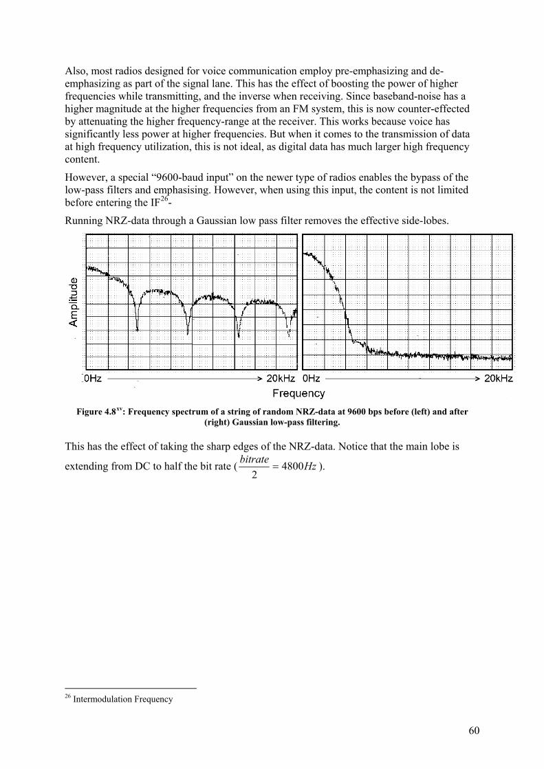
60
Also, most radios designed for voice communication employ pre-emphasizing and de-emphasizing as part of the signal lane. This has the effect of boosting the power of higher frequencies while transmitting, and the inverse when receiving. Since baseband-noise has a higher magnitude at the higher frequencies from an FM system, this is now counter-effected by attenuating the higher frequency-range at the receiver. This works because voice has significantly less power at higher frequencies. But when it comes to the transmission of data at high frequency utilization, this is not ideal, as digital data has much larger high frequency content.
However, a special “9600-baud input” on the newer type of radios enables the bypass of the low-pass filters and emphasising. However, when using this input, the content is not limited before entering the IF26-
Running NRZ-data through a Gaussian low pass filter removes the effective side-lobes.
Figure 4.8xv: Frequency spectrum of a string of random NRZ-data at 9600 bps before (left) and after
(right) Gaussian low-pass filtering. This has the effect of taking the sharp edges of the NRZ-data. Notice that the main lobe is
extending from DC to half the bit rate ( Hzbitrate
48002
).
26 Intermodulation Frequency

61
Figure 4.9xvi: Computed power spectra of MSK, BPSK and GMSK (with BT = 0.5) at 9600 bit/sec.
Comparing the power spectra’s of unfiltered MSK with BPSK and GMSK, one can see that
the main lobe of MSK-signal modulation is clearly wider than2
bitrate, as it is with BPSK and
GMSK. This simply means that MSK is not suitable for high bit rate transmission, since the bit-rate would have to be reduced to fit into the required
BPSK has a main lobe similar to GMSK, yet GMSK has even lower side-lobes. If a signal has high side-lobes means that some of the information will not be transmitted through a bandwidth-limited radio. However, the total energy-loss would be extremely small ( %1 ).
However, there are other more important reasons why I have selected GMSK as the modulation technique.
The required baseband bandwidth, and therefore the radio-channel bandwidth requirement of a GMSK system is principally determined by two factors: the data rate and the system filter's response. The response characteristic with respect to an applied data rate is referred to as the system BT (bandwidth - data rate) factor. If the BT-factor is lowered, the baseband frequency consumption is also lowered.
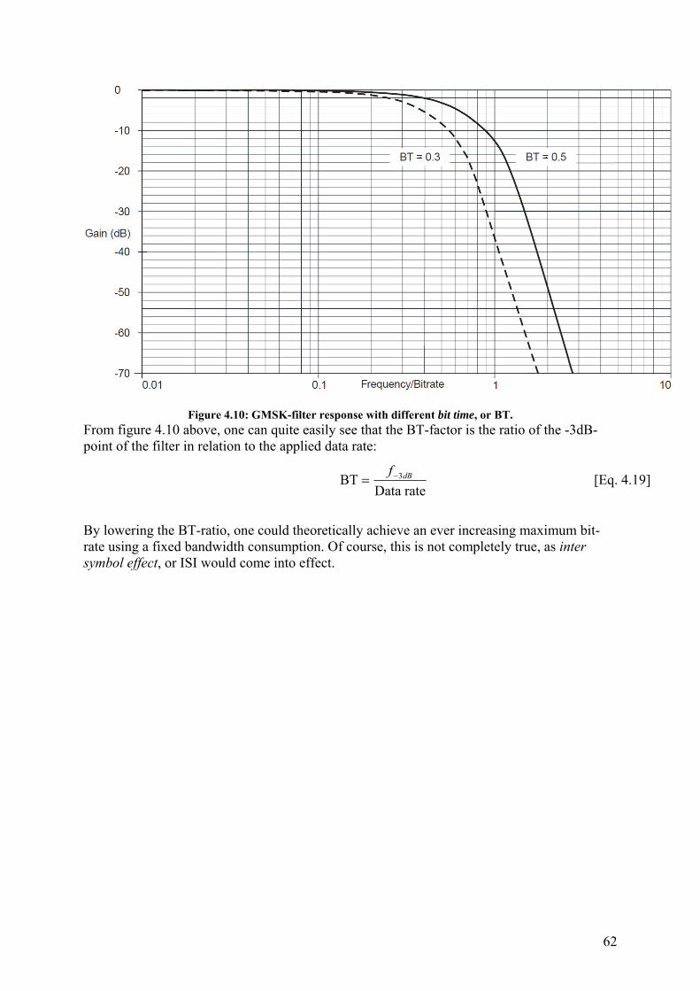
62
Figure 4.10: GMSK-filter response with different bit time, or BT.
From figure 4.10 above, one can quite easily see that the BT-factor is the ratio of the -3dB-point of the filter in relation to the applied data rate:
rateData
BT 3dBf [Eq. 4.19]
By lowering the BT-ratio, one could theoretically achieve an ever increasing maximum bit-rate using a fixed bandwidth consumption. Of course, this is not completely true, as inter symbol effect, or ISI would come into effect.

63
Figure 4.11 (left): BER performance of BPSK and GMSK w/BT=0.5 without synchronization errors. Figure 4.12 (right): BER performance of BPSK and GMSK w/BT=0.5 with varying carrier phase and symbol sync errors.
b represents the calculated values of 0N
Eb
BER is the calculated bit error ratio of the demodulators.
GMSK-modulation with a filter-value with a BT, or bit time, of 0.5 uses less bandwidth than a BPSK-signal (see figure 4.9). Still, GMSK-modulation does just as good (provides the same BER) as BPSK (figure 4.11) during no noise scenarios, and even better (provides a lower BER) than BPSK during signal noise interference (figure 4.12) and distortion.
MXCom supplies a BER vs. S/N plot that indicates typical performance, independent of bit rate (although the applied noise bandwidth is considered to match the bit rate used):
BER BER

64
Figure 4.13: Typical bit error rate for the GMSK demodulator of the CMX589A chip.
By entering data from figure 4.13 above into a list on a standard calculator (CASIO fx-9000 series) with line-fitting ability (LSQ-operation), an estimated function using exponential fit is found:
dB22.183.26dB N
SeBER
[Eq. 4.20]
This formula is used in the link budgets to find the expected BER-rate of the communication link. (See Appendix B)

65
5 Construction of the Oslo Ground Station – Remote
operation
5.1 Motivation
As the number and usage of small LEO-satellites increase, one of the key issues concerning ground stations is to get sufficient amount of data from the satellites and to the ground. There are, of course, many ways of making this happen, but on a general basis there are three main targets:
1. Increased link bandwidth. 2. Increased link-time. 3. Lowered bit error rate
Increasing the link bandwidth correlates to increasing the channel bandwidth. But as on-air frequencies are limited and shared between users across the globe, this tactic can only be stretched so far. Also, as each satellite is launched, a specific frequency and channel bandwidth is assigned by ITU, limiting the bandwidth allowed. Thus, to improve overall bandwidth to and from the satellites, one should try to maximize link-time. As a LEO-satellite orbits the earth, the amount of time it spends within “visible” range of a single spot on the ground is very limited. Also, depending on the placement of the ground station versus the inclination of the satellite orbit, the number of contacts pr day may also be very limited. For a satellite in a high inclination orbit ( i 90°), a ground station close to the equator could yield as low as 2 passes per 24-hour cycle. A steep inclination means that the satellite will pass the north and south-pole on every orbit, but as the earth is spinning in a west to east manner, each LEO-orbit would only pass a certain point on the equator a limited number of times. LEO-satellites is said to “scan” the planet as it orbits. Because of this, any ground station placed in particularly high or low latitudes, will have a significantly higher percentage of active link-time to most LEO-satellites because of the increased number of passes.
A theoretical ground station at any of the geographical poles would approximately yield 14 passes per 24-hours, depending on the altitude of the satellite. Still, assuming a maximum passage time of roughly 15 min, this would only give a link time of 210 minutes or in excess of 3 hours pr 24 hours, giving a duty-cycle of approx. 15%. Thus, using a single ground station for a single satellite would never secure “massive downloads”.
However, if one would be able to utilize multiple ground stations, located all across the globe, the transmission duty-cycle for any given satellite would be significantly higher. To achieve this, a remote operation of the satellite ground stations, most notably through an internet connection, is a must.
At the time of writing, an ESA project called the GENSO-network is in the progress of being developed. The purpose is to make a complete server/client network enabling multiple ground station to cooperate on connecting and downloading data from a myriad of LEO-satellites. However, since this system is so massive and intricate in its design, its operational date is still unclear. What this means is that it’s still is up to each satellite producer (universities and others) to ensure a method of connectivity. This normally implies a construction of a dedicated satellite ground station.

66
The University in Oslo may, in addition to the one in Oslo, at 59.9° north, place a satellite ground station at the university centre in Longyearbyen, Svalbard, at 78° north, and possibly one at the Troll research and test-drilling station, at 71° south, in the Antarctic.
What is needed is a system where multiple users can access ground stations. Moreover, this has to stable enough to reduce the need of local human interference. While remotely controlling the ground stations may become available though GENSO, this system requires a computer to run locally at each site. This may provide stability issues concerning power-outs, viruses, software updates, hang-ups and so-forth. To safely operate an instrument in a desert or remote site, the more “simple” option of directly interfacing the equipment to the internet through a microcontroller is implemented.
5.2 Tracking software
As far as these stations go, they are either controlled manually by buttons on the equipment itself, or by connecting the equipment to a computer. Most of the instruments made for satellite communication in the VHF or UHF-bands are targeted towards amateur-radio operators.
One of the easiest interfaced satellite tracking software available is a program called Orbitron27. Orbitron is a satellite tracking system for radio amateur and observing purposes. It's also used by weather professionals and other satellite communication users. It is developed and maintained by Sebastian Stoff, a radio amateur.
Figure 5.1: Screenshot of Orbitron depicting the ground station position in Oslo, Norway denoted by my
call sign LA1FRA, the link-coverage of a german CubeSat named UWE-2 (From the University of Würzburg) launched in September 2007 at an altitude of approx. 700 km.
27 Downloadable from http://www.stoff.pl/

67
Orbitron keeps updated TLEs28 from NORAD29, and can read any TLE-files supplied. To steer the elevation and azimuthal rotors, an external driver must be installed on the computer. An already developed driver called WispDDE can control the rotators used in the Oslo Satellite Ground Station via a GS-232B-controller from Yaesu. By purchasing a converter called CT-17 from ICOM, the radio can be controlled from the computer via a serial-port. With this in mind, the easiest way to implement remote control of a satellite ground station would of course be to use remote desktop or other similar programs.
However, handing out usernames and/or passwords for a networked computer is generally a no-no, so this is not an option. In addition, only one person can run interfacing programs at the same time.
To solve this, another type of architecture is needed.
5.3 Deciding on a general system
By developing a dedicated TNC30 with networking capability and adding the capability to control the rotor and radio, the ground station interfacing can be done over a network / the internet.
To achieve this, a separate Delphi-based program has been written. The program is based on a programming code supplied at Orbitrons homepage. This code is called My DDE Client 1.05, and is an empty shell that supplies the developer with a DDE31-link frond Orbitron supplying satellite-data. This is then selected as the driver for Orbitron by setting the path of the MyDDE driver in Orbitrons ‘Setup.cfg’-file.
MyDDE transmits frequency-, modulation method and rotor data to the TNC. In addition, the data to be modulated over the radio can be sent from the same computer using a mission/satellite specific program written to interface with the satellite in question. Any protocol (AX.25 or other) is sent as binary data to the TNC via UDP-packet with a specific data header at the beginning of the data-field.
28 The North American Aerospace Defense Command (NORAD) developed the Two-Line Element (TLE) format for transmitting satellite Keplerian elements.Using these, the position of a satellite can be computed by a satellite tracking program. The Kepplerian elements are normally accurate enough within a time-window of approx. 2 weeks. 29 North American Aerospace Defense Command 30 Terminal Node Controller. Cconsist of a modulator/demodulator for digital radio operation, and a computer interface 31 Dynamic Data Exchange. A Windows-compatible way of transmitting data from one program to another without using files.
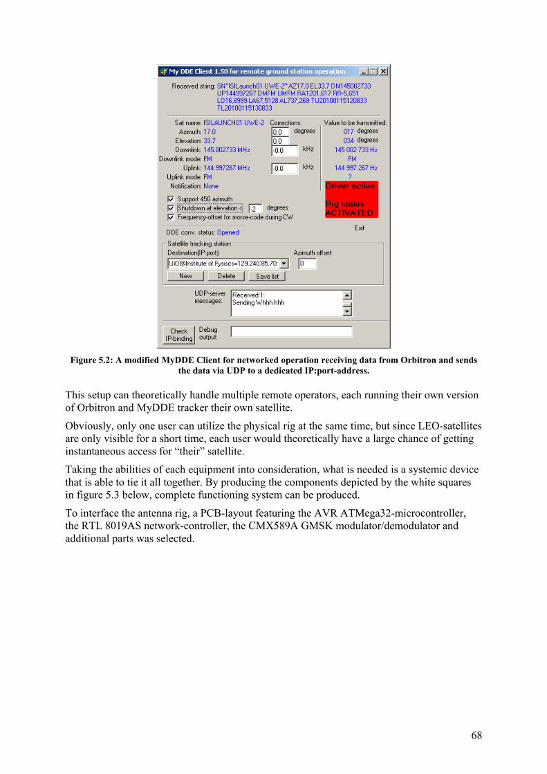
68
Figure 5.2: A modified MyDDE Client for networked operation receiving data from Orbitron and sends
the data via UDP to a dedicated IP:port-address. This setup can theoretically handle multiple remote operators, each running their own version of Orbitron and MyDDE tracker their own satellite.
Obviously, only one user can utilize the physical rig at the same time, but since LEO-satellites are only visible for a short time, each user would theoretically have a large chance of getting instantaneous access for “their” satellite.
Taking the abilities of each equipment into consideration, what is needed is a systemic device that is able to tie it all together. By producing the components depicted by the white squares in figure 5.3 below, complete functioning system can be produced.
To interface the antenna rig, a PCB-layout featuring the AVR ATMega32-microcontroller, the RTL 8019AS network-controller, the CMX589A GMSK modulator/demodulator and additional parts was selected.

69
Figure 5.3: General system overview, with remote operation connectivity
Notice that since the ATMega32-chip only has a single UART-module, the serial output is shared between the RS-232B rotor controller and the CI-V interface for the ICOM radio. This is possible because ICOM radios only listens to packets preceded by their own address. By transmitting the packet termination-code at the end of all data destined for the RS-232B, and opposite when transmitting to the ICOM, each component will only accept data targeted for them selves.
Rs-232
Internet Computers
w/satellite tracking software
Micro-controller
UDP
UDP
CI-V PTT
AUDIO/GMSK
RS-232B
Rotor-Controller
azimuth elevation
LNAs
UHF VHF
GMSK modem
Tx Clk
Tx Data
Rx Clk
Rx Data
Tx Enable
Level convert
Network-Controller
Networked driver

70

71
5.4 The ICOM 910h transceiver
5.4.1 Connectors
Figure 5.4xvii: Part of IC-910h schematics showing ACC (1) and DATA-sockets (2)
with inductors (3) and capacitors (4).
As can be seen from figure 5.4 above, no input or output connections are directly AC-coupled. This is a good thing, as long strings 0’s or 1’s may require that the baseband-modulating input-signal must be DC-coupled to prevent voltage drifts. Because of this, great caution must be taken to insure that ground loops, either though power supply or signal cables, are not created when connecting external equipment. In this project, the terminal node controller, or TNC, is constructed so that one can:
Let the radio and the TNC share a common power-supply and be fully DC-coupled.
Set the TNC in AC-mode to prevent ground loops when having separate power-supplies. This requires that the digital data must be scrambled before modulation.
Or disconnect the signal ground between the TNC and the radio to let the ground-loop act as the common ground. This is a last resort measure that should be avoided.
2
1
3
4

72
When it comes to high frequency content, it seems that all of ICOM 910h’s connector-lines have an LC-filter consisting of a coil (100 μF) and a capacitor. Assuming that any connected line has a series resistance of at least 2kΩ, this would act as a RLC low-pass filter.
The cut-off frequency Cf of the RLC-setup is easily calculated using the formula:
LC
fC
2
1 [Eq. 5.1]
ICOM has not specified the value of all their capacitors, but with the capacitor on the data out line (DOUT), the capacitor-value of 47 pF can be read out clearly. This gives a cut-off frequency of:
MHzLC
fC 3.2103.4
1
10472
1
2
1716
[Eq. 5.2]
This frequency-limit is way above what will be produced by any modulator used for communication at these frequencies. Assuming that the other capacitors has a comparable value, one can conclude that these are obviously put there to protect against voltage spikes and static electricity, and not to implement any kind of frequency limiting limit.
5.4.2 ICOM 910h functions
Figure 5.5: The ICOM 910h receiver construction layout.
Normally, with radios prepared for voice-communication, several techniques are applied to improve vocal communication. In the transmitter part, the modulating signal is subject to pre-emphasizing, gain adjustment and low-pass filtering. This is not suitable for higher baud-rate transmissions. The ICOM 910h features support for higher baud-rates using a separate unfiltered signal lane.
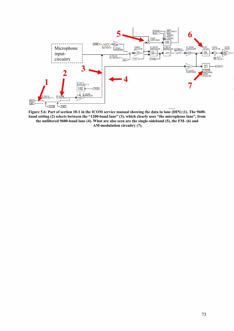
73
Figure 5.6: Part of section 10-1 in the ICOM service manual showing the data in lane (DIN) (1). The 9600-baud setting (2) selects between the “1200-baud lane” (3), which clearly uses “the microphone lane”, from
the unfiltered 9600-baud lane (4). What are also seen are the single-sideband (5), the FM- (6) and AM-modulation circuitry (7).
1 2
5 6
7
3 4
Microphone input-circuitry
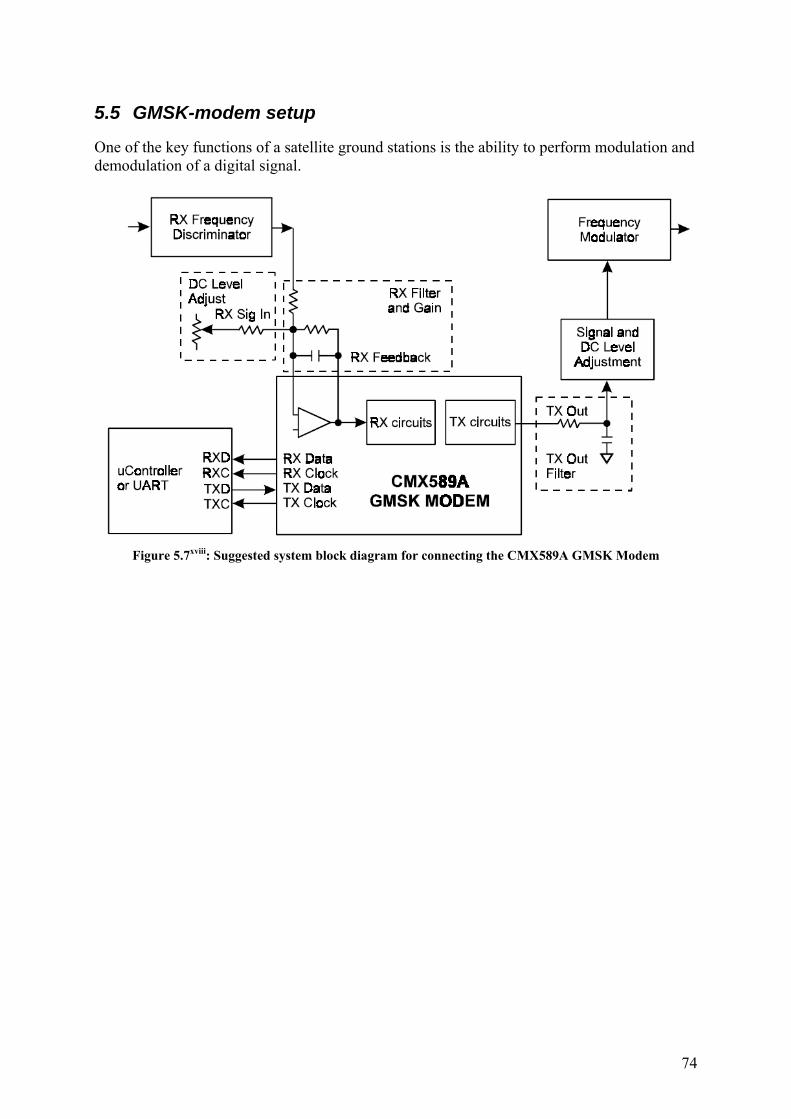
74
5.5 GMSK-modem setup
One of the key functions of a satellite ground stations is the ability to perform modulation and demodulation of a digital signal.
Figure 5.7xviii: Suggested system block diagram for connecting the CMX589A GMSK Modem

75
5.5.1 DOC1 & DOC2 capacitors The formula for calculation of the capacitors that is to be connected to the Rx dc-level measurement-module is not part of the datasheet. However, several baud rates versus capacitor-values are listed. From these values one can see that for every time you double the baud-rate, the capacitance is halved. So a generic formula can be found:
bitrateSelected
kbitsFCC
_
4*030.08|7 [Eq. 5.3]
As we select a baud rate of 9600, the result is then:
nFFkbits
kbitsFCC 5.120125.0
6.9
4*030.08|7 [Eq.5.4]
Unfortunately, only 10 and 15nF capacitors can be bought, so as smaller capacitance probably relates to a higher cut-off frequency in the DC-measurement circuitry, two 10nF capacitors are selected.
Figure 5.8xviii: Block diagram of CMX589AD

76
5.6 The remotely operated satellite ground station controller
Designing a PCB-layout in CADSTAR32, the design (See Appendix C and D) was sent abroad for production. The resulting two-layer printed circuit-board was fitted with solder-paste using a metal-stencil and the surface-mounted components were soldered using a gas-vapour soldering machine. Later the hole-mounted components were fitted, and the device connected to the ground station equipment (see figure 5.10).
Figure 5.9: The resulting remote satellite ground station controller version 1.99 depicting the connectors (from top left to right) for Ethernet connector (1), ICOM data-modulation connector (2) for both main
and sub-lane GMSK, AFSK and Morse-keying operation., UART-connector (3) for RS-232B control and a CI-V connector (4) for radio frequency control. The microcontroller-chip (5) and the GMSK
modulator/demodulator (6) can be seen in the middle.
32 A design editor produced by Zuken Ltd.
21 3 4
6
5

77
Figure 5.10: Showing the remote satellite ground station controller in a system setup.

78
6 Conclusions
This thesis clearly states that the implementation of a remotely operated ground station is not only possible, but a goal that should be aimed for by all ground station constructers. Cooperation between ground stations provides strong benefits when it comes to downloading data from LEO-satellites due to the increase of link-time. However, this is clearly limited by the fact that not only are there multiple ways of modulating a baseband signal, but there is also a multitude of ways of implementing a satellite communications protocol. Because of this, the suggestion is made to implement all ground stations so that they may act in a binary mode. Using this mode, each satellite producer/ground station user can program their specific codes in their own program locally. This program then communicates with the satellite through the ground station using, for example, the UDP-protocol across the internet. This master thesis shows that a microcontroller, with some extra components, is capable of performing such a service.
6.1 Achievements
The Oslo Satellite Ground Station is up and running, and has received Morse-coded messages from several satellites. So far no data communication has been achieved, but this is because of a lack of implemented data protocol towards satellites in space.
The rotor and radio is operated using the Remote Satellite Ground Station Controller produced in this thesis, and the functionality to transmit and receive GMSK through radio is implemented.
Multiple segments in the design of the schematics produced in this master thesis can be reused in the design of a communication-module aboard a CubeSat satellite, and thus facilitates the future construction of the CubeStar.
6.2 Future work
The networked microcontroller of the ground station, with its simplistic UDP-protocol, can easily be controlled though a driver attached to a GENSO-server. It is therefore possible to connect the Oslo Ground Station to the GENSO network. Also, by programming the microcontroller with a standard communication-protocol, less programming will have to be done at the ground station user side.

79
7 List of references I http://scienceworld.wolfram.com/physics/MaxwellEquations.html, 2009-10-15 II http://scienceworld.wolfram.com/physics/MaxwellEquations.html, 2009-10-15 III Tipler, Paul (2004). Physics for Scientists and Engineers: Electricity, Magnetism, Light, and Elementary Modern Physics (5th ed.). W. H. Freeman. ISBN 0-7167-0810-8. IV Golo, G. and Talasila, V. and Schaft van der, A.J. (2002) Approximation of the telegrapher's equations. In: 41st IEEE Conference on Decision and Control, 2002, Las Vegas, Nevada, U.S.A. V “Handbook of Linear Partial Differential Equations for Engineers and Scientists” by Andrei D. Polyanin, ISBN:9781584882992, pub. Nov 28, 2001. VI Wikipedia, http://en.wikipedia.org/wiki/Isotropic_radiator , 2009-11-18 VII http://en.wikipedia.org/wiki/File:Dipole_Antenna.jpg, 2009-11-19 VIII NBS TECHNICAL NOTE 688 – Yagi Antenna Design, issued dec. 1976. http://tf.nist.gov/timefreq/general/pdf/451.pdf, 2009-11-28 IX The article “Why 50Ohms?”, http://www.microwaves101.com/encyclopedia/why50ohms.cfm, 2009-12-08 X http://sv1bsx.50webs.com/antenna-pol/polarization.html, 2009-11-16 XI W. L. Stutzman and G. A. Thiele, Antenna Theory and Design, John Wiley & Sons, New York, 1981. XII General Conference, Davos, 11 to 16 September 2005, Definition of Modes: NBFM, Paper number: 17, International Amateur Radio Union Region 1,http://www.rsgb-spectrumforum.org.uk/Papers/VHF/Davos%20C5%20Papers/DV05_C5_17%20SARL%20NBFM.pdf XIII Communication Theory, by T G Thomas S Chandra Sekhar. http://books.google.no/books?id=C1C6IBiCoXsC&lpg=PA238&ots=v2FG2n66zg&dq=FM%20threshold%20vs%20SNR&pg=PA238#v=onepage&q=&f=false page 238. ISBN 0070590915, 9780070590915, publisher: Tata McGraw-Hill, 2005 XIV Wikipedia, Non-return-to-zero, http://en.wikipedia.org/w/index.php?title=Non-return-to-zero&oldid=334853041 (last visited Jan. 11, 2010) XV APPLICATION NOTE, MX589 GMSK MODEM Application, MX589_GMSK_Application.pdf.. XVI THRESHOLD DETECTION PERFORMANCE OF GMSK SIGNAL WITH BT==O.5 by Gee L. Lui at The Aerospace Corporation, Communication Systems Engineering Department. El Segundo, California. http://www.argreenhouse.com/society/TacCom/papers98/15_02i.pdf

80
XVII ICOM 910H service-manual, S-13714HZ-C1 © 2001 Icom Inc. Cut-out from page 99, chap 12-5: MAIN UNIT (1),.. XVIII Cut-out from page 3 of CMX589A data sheet. XIXSSB Electronic USA. LNA specs. http://www.ssbusa.com/gaasfet.html

81
Glossary of terms and acronyms AFSK Audio Frequency-shift keying.
AM Amplitude modulation.
BPSK Binary phase-shift keying.
BT Bit-Time, see Eq. 4.19 on page 62.
FM Frequency modulation.
FSK Frequency shift keying.
GMSK Gaussian minimum shift keying.
PM Phase modulation.
QPSK Quadrature phase-shift keying.
EIRP Equivalent Isotropically Radiated Power (Combined power and antenna gain).
G/T Gain to noise temperature ratio (Of a receiving system).
LSQ Least square fit. A linear algebraic procedure to fit a line or formula to a set of
samples.
TNC Terminal Node Controller. A device that modulates a digital baseband signal for
radio transmission.
VSWR Voltage Standing Wave Ratio. A way of measuring the magnitude of signal
reflection.

82
8 List of tables
TABLE 2.1: MAXWELL’S WAVE-EQUATIONS WHEN IN ABSENCE OF POLARISABLE MEDIA. ........ 12 TABLE 2.2: MAXWELL WAVE-EQUATIONS WHEN IN PRESENCE OF POLARISABLE MEDIA ......... 12 TABLE 3.1: QUARTER WAVE-LENGTH CALCULATIONS ......................................................................... 43 TABLE 3.2: APPROXIMATE LOSSES, IN DB, ARISING FROM ANTENNA-SIGNAL POLARIZATION
MISMATCH ............................................................................................................................................... 45 TABLE 3.3: CALCULATING THE REQUIRED LENGTHS OF THE PHASE-STUBS................................... 47 TABLE 4.1: LIST OF STANDARD BANDWIDTHS......................................................................................... 56

83
9 Table of figures
FIGURE 2.1: ELECTRIC FIELD (E) DUE TO POINT CHANGES................................................................... 11 FIGURE 2.2: MAGNETIC FIELD (H) DUE TO MOVING CHARGE IN A CONDUCTOR............................ 11 FIGURE 2.3: DEPICTING A LIGHT-BEAM AS A SERIES OF PERPENDICULAR MAGNETIC AND
ELECTRIC FIELDS. .................................................................................................................................. 13 FIGURE 2.4: ELEMENTARY COMPONENTS OF A TRANSMISSION LINE............................................... 14 FIGURE 2.5: A SIMPLE MODEL OF A TRANSMISSION LINE..................................................................... 14 FIGURE 2.6: LOOKING AT THE TRANSMISSION LINE WITH RESPECT TO VOLTAGE, TIME AND
PLACEMENT X.......................................................................................................................................... 15 FIGURE 2.7: THE CONSTRUCTION (A), VISUALIZATION OF THE E-FIELD (B) AND THE MAGNETIC
FIELD (C) IN A TWO-WIRE SETUP........................................................................................................ 17 FIGURE 2.8: VISUALIZATION OF THE E-FIELD (A) AND THE MAGNETIC FIELD (B) IN A COAXIAL
DESIGN. ..................................................................................................................................................... 17 FIGURE 2.9: THE SIGNAL REFLECTION GAINS A 180° PHASE SHIFT WHEN GOING FROM
RELATIVELY HIGH IMPEDANCE TO LOWER IMPEDANCE............................................................ 18 FIGURE 2.10: THE SIGNAL REFLECTION HAS NO PHASE SHIFT WHEN GOING FROM RELATIVELY
LOW IMPEDANCE TO HIGHER IMPEDANCE. .................................................................................... 18 FIGURE 2.11: THE THEORETICAL ISOTROPIC RADIATOR....................................................................... 19 FIGURE 2.12: RADIO WITH SHORT ENDED OUTPUT ................................................................................. 20 FIGURE 2.13: A RADIO WITH A SHORT ENDED OUTPUT, FORMING STANDING WAVES. BECAUSE
THE DISTANCE BETWEEN THE CONDUCTORS IS NONE-ZERO, SOME ELECTRIC AND MAGNETIC FIELDS DOES RADIATE FROM THE CABLE END, BUT THESE FIELDS TEND TO CANCEL EACH OTHER OUT AS THEY MOVE AWAY FROM THE CABLE END. ......................... 21
FIGURE 2.14: MAKING A DIPOLE ANTENNA FROM TWO ANGLED WIRES.......................................... 22 FIGURE 2.15: CURRENT DISTRIBUTION ON A SHORT DIPOLE ............................................................... 23 FIGURE 2.16: EMISSION DIAGRAM OF A SHORT DIPOLE TAKES THE FORM OF A TORUS.............. 23 FIGURE 2.17: CONSTRUCTION OF A HALF-WAVE DIPOLE ANTENNA FROM TWO ANGLED WIRES
..................................................................................................................................................................... 25 FIGURE 2.18: MAXIMUM VOLTAGE ACROSS A DIPOLE .......................................................................... 25 FIGURE 2.19: MAXIMUM CURRENT ACROSS A DIPOLE........................................................................... 25 FIGURE 2.20: CROSS SECTION OF THE FAR-FIELD EMISSION DIAGRAM OF THE HALF-WAVE
DIPOLE COMPARED TO ......................................................................................................................... 26 FIGURE 2.21: SIMPLE YAGI SETUP................................................................................................................ 27 FIGURE 2.22: CROSS SECTION OF A 2-ELEMENT REFLECTOR-YAGI EMISSION DIAGRAM
DEPICTING THE MAIN AND BACK LOBE........................................................................................... 27 FIGURE 2.23: GAIN IN DB OF A 2-ELEMENT YAGI RELATIVE TO A SINGLE DIPOLE WHEN
VARYING ELEMENT SPACING ............................................................................................................. 28 FIGURE 2.24: CROSS SECTION OF A 2-ELEMENT DIRECTOR-YAGI EMISSION DIAGRAM
DEPICTING THE MAIN AND BACK LOBE........................................................................................... 28 FIGURE 2.25: A YAGI-UDA ARRAY CONSISTS OF A REFLECTOR (1) THE DIPOLE (2) AND A
NUMBER OF DIRECTORS (3...K) ........................................................................................................... 29 FIGURE 2.26: SHOWING THE VARIATION OF THE E-FIELD USING VERTICAL (1) AND
HORIZONTAL (2) POLARIZATION........................................................................................................ 30 FIGURE 2.27: SHOWING THE VARIATION OF THE E-FIELD WHEN RECEIVING A LEFT HAND
CIRCULAR POLARIZATION (LHCP) AND RIGHT HAND CIRCULAR POLARIZATION (RHCP). 30 FIGURE 3.1: THE ANTENNA TOWER (1) WITH THE MAIN VERTICAL POLE (2), THE CROSS-BAR (3),
..................................................................................................................................................................... 36 FIGURE 3.2: BOTTOM- SIDE PICTURE OF THE TOP ATTACHMENT PIECE (1), THE REAR END OF
THE FRONT ANTENNA BOOM (2) AND THE CUSTOM MADE ALUMINIUM PIECE WITH SCREW-HOLES (3). .................................................................................................................................. 39
FIGURE 3.3: INSERTING THE CUSTOM ALUMINIUM PIECE .................................................................... 39 FIGURE 3.4: DEPICTING THE TOP ATTACHMENT PIECE (1) WITH INSERTED SCREWS, THE LOVER
ATTACHMENT PIECE (2), THE REAR END OF THE FRONT ANTENNA BOOM (3), THE FRONT END OF THE REAR ANTENNA BOOM (4) AND THE RIG SUPPORTING CROSS-BAR (5). .......... 39
FIGURE 3.5: CABLE LOSS VERSUS IMPEDANCE, IN A COPPER COAX WITH A 10MM DIAMETER. 40 FIGURE 3.6: MAXIMUM POWER AND VOLTAGE HANDLING OF A 10 MM AIR FILLED COAX
(INTERNAL VOLTAGE BREAK-DOWN AT 100 000 V/M).................................................................. 41 FIGURE 3.7: IMPEDANCE MATCHING OF A 1:2 SPLIT............................................................................... 42

84
FIGURE 3.8: TWO IMPEDANCE-SPLITS (1) GOING FROM RG-213 CABLE (2) TO PAIRS OF RG-11 CABLES WITH QUARTER-WAVE LENGTHS. THE SECOND SPLIT HAS BEEN COVERED WITH SELF-SEALING TAPE AND IS READY FOR OUTDOOR USE. ........................................................... 44
FIGURE 3.9: REAR VIEW OF CROSSED DIPOLES DEPICTING PHASING-REQUIREMENTS OF RHCP AND LHCP. ................................................................................................................................................ 46
FIGURE 3.10: INTRODUCING EXTRA PHASING STUBS TO ENSURE CORRECT POLARIZATION..... 46 FIGURE 3.11: THE COPPER CORE OF THE WESTFLEX103 (1) IS TOO WIDE TO BE INSERTED INTO
THE CONNECTOR TIP (2). IT HAD TO BE MADE SMALLER BY CUTTING ALONGSIDE THE CENTRE-LEAD WITH A PAIR OF CUTTING PLIERS (3), DECREASING THE EFFECTIVE DIAMETER OF THE CENTRE-LEAD. .................................................................................................... 48
FIGURE 4.1: FLUX DENSITY PRODUCED BY AN ISOTROPIC SOURCE.................................................. 50 FIGURE 4.2: POWER RECEIVED BY AN IDEAL ANTENNA WITH AN AREA A. .................................... 51 FIGURE 4.3: A SATELLITE LINK FEATURING AN LNA, OR LOW NOISE AMPLIFIER. NOTICE THAT
BOTH raL AND taL OFTEN INCLUDES EVENTUAL CABLE-LOSS FROM THE ANTENNA TO THE
LNA, OR FROM THE PA, THE POWER AMPLIFIER, TO THE ANTENNA......................................... 54 FIGURE 4.4: SIMPLIFIED EARTH GROUND STATION RECEIVER. BPF IS BAND PASS FILTER. .......... 54 FIGURE 4.5: DOUBLE CONVERSION EARTH STATION RECEIVER. THE FIRST DOWNCONVERSION
SHIFTS SIGNALS IN A 500 MHZ BAND TO THE FIRST 900-1400 MHZ. THE SECOND DOWNCONVERTER HAS A TUNEABLE LOCAL OSCILLATOR AND CHANNEL SELECTION FILTER TO SELECT THE WANTED RADIO CHANNEL/FREQUENCY IN THE SECOND IF CENTERED AT 70 MHZ. .......................................................................................................................... 55
FIGURE 4.6: NOISE MODEL OF A RECEIVER............................................................................................... 57 FIGURE 4.7: NRZ-DATA.................................................................................................................................... 59 FIGURE 4.8: FREQUENCY SPECTRUM OF A STRING OF RANDOM NRZ-DATA AT 9600 BPS BEFORE
(LEFT) AND AFTER (RIGHT) GAUSSIAN LOW-PASS FILTERING. ................................................. 60 FIGURE 4.9: COMPUTED POWER SPECTRA OF MSK, BPSK AND GMSK (WITH BT = 0.5) AT 9600
BIT/SEC. ..................................................................................................................................................... 61 FIGURE 4.10: GMSK-FILTER RESPONSE WITH DIFFERENT BIT TIME, OR BT. ..................................... 62 FIGURE 4.11 (LEFT): BER PERFORMANCE OF BPSK AND GMSK W/BT=0.5 WITHOUT
SYNCHRONIZATION ERRORS............................................................................................................... 63 FIGURE 4.12 (RIGHT): BER PERFORMANCE OF BPSK AND GMSK W/BT=0.5 WITH VARYING
CARRIER PHASE AND SYMBOL SYNC ERRORS. .............................................................................. 63 FIGURE 4.13: TYPICAL BIT ERROR RATE FOR THE GMSK DEMODULATOR OF THE CMX589A CHIP.
..................................................................................................................................................................... 64 FIGURE 5.1: SCREENSHOT OF ORBITRON DEPICTING THE GROUND STATION POSITION IN OSLO,
NORWAY DENOTED BY MY CALL SIGN LA1FRA, THE LINK-COVERAGE OF A GERMAN CUBESAT NAMED UWE-2 (FROM THE UNIVERSITY OF WÜRZBURG) LAUNCHED IN SEPTEMBER 2007 AT AN ALTITUDE OF APPROX. 700 KM. ............................................................ 66
FIGURE 5.2: A MODIFIED MYDDE CLIENT FOR NETWORKED OPERATION RECEIVING DATA FROM ORBITRON AND SENDS THE DATA VIA UDP TO A DEDICATED IP:PORT-ADDRESS. . 68
FIGURE 5.3: GENERAL SYSTEM OVERVIEW, WITH REMOTE OPERATION CONNECTIVITY ........... 69 FIGURE 5.4: PART OF IC-910H SCHEMATICS SHOWING ACC (1) AND DATA-SOCKETS (2) WITH
INDUCTORS (3) AND CAPACITORS (4)................................................................................................ 71 FIGURE 5.5: THE ICOM 910H RECEIVER CONSTRUCTION LAYOUT...................................................... 72 FIGURE 5.6: PART OF SECTION 10-1 IN THE ICOM SERVICE MANUAL SHOWING THE DATA IN
LANE (DIN) (1). THE 9600-BAUD SETTING (2) SELECTS BETWEEN THE “1200-BAUD LANE” (3), WHICH CLEARLY USES “THE MICROPHONE LANE”, FROM THE UNFILTERED 9600-BAUD LANE (4). WHAT ARE ALSO SEEN ARE THE SINGLE-SIDEBAND (5), THE FM- (6) AND AM-MODULATION CIRCUITRY (7). ............................................................................................................. 73
FIGURE 5.7: SUGGESTED SYSTEM BLOCK DIAGRAM FOR CONNECTING THE CMX589A GMSK MODEM...................................................................................................................................................... 74
FIGURE 5.8: BLOCK DIAGRAM OF CMX589AD........................................................................................... 75 FIGURE 5.9: THE RESULTING REMOTE SATELLITE GROUND STATION CONTROLLER VERSION
1.99 DEPICTING THE CONNECTORS (FROM TOP LEFT TO RIGHT) FOR ETHERNET CONNECTOR (1), ICOM DATA-MODULATION CONNECTOR (2) FOR BOTH MAIN AND SUB-LANE GMSK, AFSK AND MORSE-KEYING OPERATION., UART-CONNECTOR (3) FOR RS-232B CONTROL AND A CI-V CONNECTOR (4) FOR RADIO FREQUENCY CONTROL. THE MICROCONTROLLER-CHIP (5) AND THE GMSK MODULATOR/DEMODULATOR (6) CAN BE SEEN IN THE MIDDLE............................................................................................................................. 76

85
FIGURE 5.10: SHOWING THE REMOTE SATELLITE GROUND STATION CONTROLLER IN A SYSTEM SETUP......................................................................................................................................................... 77


10 Appendix A - UDP command protocol description
Command protocol description for remote TNC-operation through UDP data packets at port 45963 The hex-values describes the initial values required in the UDP-data field: PC->Ctr UDP: 0x00 Status req Ctr Status Standby: Ctr->PC UDP: 0x00 Ctr Status LockedToRequestingIP(operational): Ctr->PC UDP: 0x01 Ctr Status LockedToOtherIP(busy): Ctr->PC UDP: 0x0E +LockedIP[4] PC->Ctr UDP: 0x01 RequestLock Status LockedToRequestingIP(operational,OK): Ctr->PC UDP: 0x01 Status LockedToOtherIP(busy, notOK): Ctr->PC UDP: 0x0E PC->Ctr UDP: 0xhhhh hhhh (when length <= 8) if(LockedToRequestingIP) then Ctr outputs the following sequence to the UART: 0xhhhh hhhh 0D else if(Standby) then Ctr Status LockedToRequestingIP(operational): Ctr outputs the following sequence to the UART: 0xhhhh hhhh 0D else drops packet PC->Ctr UDP: 0xhhhh hhhh hhhh h..... (when length > 8) if(LockedToRequestingIP) then Ctr outputs the following sequence to the UART: 0xhhhh hhhh 0D hhhh h.... OD else if(Standby) then Ctr Status LockedToRequestingIP(operational): Ctr outputs the following sequence to the UART: 0xhhhh hhhh 0D hhhh h.... OD else drops packet PC->Ctr UDP: 0x02 ReleaseLock if(LockedToRequestingIP) then Status Standby(released): Ctr->PC UDP: 0x00 else drops packet If no packet has been received for approx. 1min, then Ctr Status Standby: Ctr->PC UDP: 0x00


Appendix B – Estimated satellite communication link-budget
CubeStar – Oslo Ground Station using GMSK
Fysisk Institutt Date : 02/12/2009 Broadend values are calculated using worksheet functions. STATIONS :OSLO (Tx) OSLO (Rx) Normal texted values are entered by hand Version DLL Propagation : 20060213
Parameters The Satellite
Satellite Latitude (°) 47,2000 North/south
Satellite Longitude (°) 27,6768 East/west
Satellite height (km) 700,0000
TX Station Oslo Satellite Ground Station
Latitude (°) 59,9370 Longitude (°) 10,7181 Height (km) 0,0900 Antenna Diameter (m) 0,5000 Antenna Efficiency (%) 60,0000 Polarisation (circular = 45°) (°) 45,0000 Satellite Elevation (°) 5,0609 Distance (km) 2557,5843
RX Station Oslo Satellite Ground Station
Latitude (°) 59,9370 Longitude (°) 10,7181 Height (km) 0,1150 Satellite Elevation (°) 5,0609 Distance (km) 2557,5843
Satellite link
Baud rate 9600 Modulation (bits per symbol) 1,0 AFSK/MSK/BPSK/GMSK FEC rate 1,0 Usefull Bit rate (Mbps) 0,0096 Uplink Frequency (GHz) 0,4330 Uplink channel separation (Hz) 25 000 Standard FM has 25kHz ch. separation. NFM has 12,5 Uplink peak frequency deviation (Hz) 5 000 Uplink, minimum RF BW consumption (Hz) 19 600 Downlink Frequency (GHz) 0,4330 Downlink channel separation (Hz) 25 000 Standard FM has 25kHz ch. separation. NFM has 12,5 Downlink peak frequency deviation (Hz) 5 000 Downlink,minimum RF BW consumption (Hz) 19 600 Uplink Availability (%) 12,0 Downlink Avalability (%) 12,0

90
Uplink (station to satellite)
Tx station Power OSLO ground station
Amplifier Power (dBW) 17,0 50 W Feeder Losses (dB) 5,5 Loss over entire cable stretch,+J105 70 meters Pointing error loss(+-10degrees) (dB) 0,5 Max. Antenna Gain (dBic) 14,4 Tonna (F9FT) 20438 (16dBi) - alu. cross bar loss (1,6) EIRP (dBW) 25,4
Propagation losses
Free Space Losses (dB) 153,3 Atm. Gaz Attenuation (dB) 0,00000 Low value due to low frequency Rain Attenuation (dB) 0,00000 Low value due to low frequency Clouds Attenuation (dB) 0,00000 Low value due to low frequency Scintillation (dB) 0,00000 Low value due to low frequency Polarisation Losses (dB) 3,0 Accounts for linear->RHCP ant.polarization mismatch Total Losses (dB) 156,3
Satellite Rx Parameters Satellite Rx Satellite Antenna Gain (footprint edge)
(dBic) 0,0
Feeder Losses (dB) 0,4 Estimated Feeder Noise Temperature (K) 150,0 Rx Noise Figure (dB) 1,0 Unknown Rx Noise Temperature (dBK) 25,9 Rx Satellite Noise Figure : G/T (dB/K) -25,9
Uplink link budget
(C/N0) uplink (dBHz) 71,8 Calculated using total loss (C/I) uplink (dB) 30,0 Assumed 1000:1 signal/interference ratio (Eb/N0) uplink (dB) 32,0 Implementation Losses (dB) 1,0 Estimated (C/N) downlink (dB) -3,2 FM demodulator threshold (dB) 12,0 Assumed FM-demodulator threshold Threshold margin (dB) -100,0 Must be above 0 dB to avoid threshold deterioration! Margin (dB) 34,1567 Good signal margin in uplink!

91
Downlink (Satellite to station)
Tx Satellite Power Satellite
Amplifier Power (dBW) -3,0 0,5 W max = 0dBW = 1W Feeder Losses (dB) 0,4 Loss before the LNA Tx Satellite Antenna Gain (footprint edge)
(dBic) 0,0 Dipole with unknown orientation->"Isotrophic"
EIRP (dBW) -3,4
Propagation Losses
Free Space Losses (dB) 153,3281 Atm. Gaz Attenuation (dB) 0,0000000 Low value due to low frequency Rain Attenuation (dB) 0,0000000 Low value due to low frequency Clouds Attenuation (dB) 0,0000000 Low value due to low frequency Scintillation (dB) 0,0000000 Low value due to low frequency Polarisation Losses (dB) 3,0 Accounts for linear->RHCP ant.polarization mismatch Total Losses (dB) 156,3
Rx Parameters OSLO ground station
Rx Station Antenna gain (dBic) 14,4 Tonna (F9FT) 20438 (16dBi) - alu. cross bar loss (1,6)
Clear Sky Noise Temperature (K) 61,1 Ground Noise Temperature (K) 290,0 Feeder Noise Temperature (K) 290,0
http://webs.uvigo.es/servicios/biblioteca/uit/rec/P/R-REC-P.372-9-200708-I!!PDF-E.pdf page 8 RECOMMENDATION ITU-R P.372-9
Feeder Losses (dB) 1,6 Estimated from cable lengths befor LNA vs loss/meter Rx Noise Figure (dB) 0,9 Noise figure from SSB SP-7000 preamp spec. Rx Noise Temperature (clear sky) (dBK) 27,6 Rx Noise Temperature (rain/clouds) (dBK) 27,6 Rx station Noise Figure : G/T (dB/K) -13,2
Downlink link budget
(C/N0) downlink (dBHz) 55,7 Signal - total loss + G/T + Boltzmanns constant (C/I) downlink (dB) 30,0 1000:1 signal/interference ratio assumed (Eb/N0) downlink (dB) 15,8 Implementation Losses (dB) 1,0 (C/N) downlink (dB) 11,7 Above threshold FM demodulator threshold (dB) 10,0 Standard FM discriminator (PLL) threshold Threshold margin (dB) 1,7 Must be above 0 dB to avoid threshold deterioration! S/N @ 100% mod (dB) 18,8 S/N @ 80% mod (dB) 16,8
Expected BER using GMSK @ 80% (dB) 3,2E-08 More than good enough bit-error rate at 0.5W


Appendix C – Satellite Ground Station Remote Controller - Schematics
Schematics 1: TOP schematic drawing

94
Schematics 2: Power and bypass capacitors

95
Schematics 3: GMSK modem setup

96
Schematics 4: RS-232 and CI-V driver and level-conversion circuits
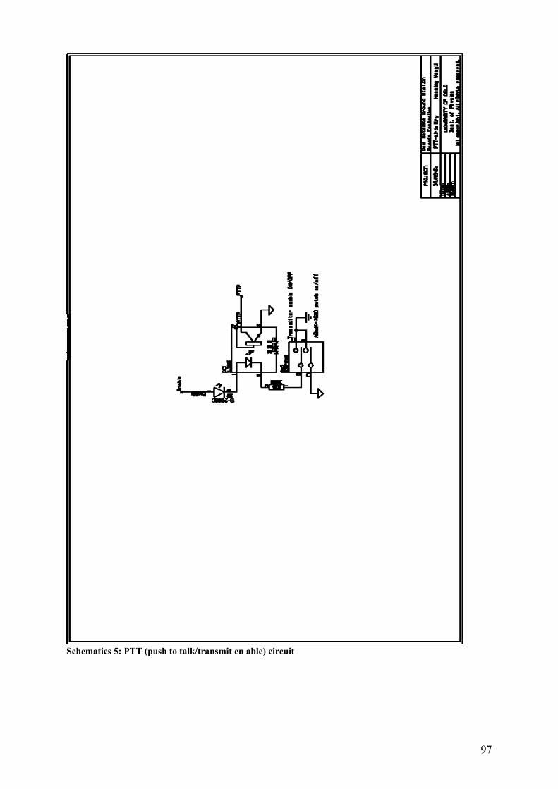
97
Schematics 5: PTT (push to talk/transmit en able) circuit

98
Schematics 6: PWM low-pass and driver circuitry

99
Schematics 7: Reset button

100
Schematics 8: Network controller

101
Schematics 9: Weak drive block (to separate programming interface from IO-lines during programming)


Appendix D - Satellite Ground Station Remote Controller – PCB-layout
PCB-layout 1: All layers (normal)

104
PCB-layout 2: BOTTOM electric

105
PCB-layout 3: TOP electric


Appendix E – Source code for
micro-controller on ground
station controller circuit board
(c-code for AVR ATMEGA32)
easyethavr.c ////////////////////////////////////////////////////////////////////// // REALTEK RTL8019AS DRIVER FOR AVR ATMEGA163 // PACKET WHACKER ENABLED // Author: Fred Eady // Company: EDTP Electronics // Version: 1.2 // Date: 08/08/19 // Description: ARP, PING, ECHO and LCD Control, TCP, UDP ////////////////////////////////////////////////////////////////////// //****************************************************************** //* PORT MAP //****************************************************************** // PORT A = rtldata - data bus RTL8019 and AVR // 0 SD0 // 1 SD1 // 2 SD2 // 3 SD3 // 4 SD4 // 5 SD5 // 6 SD6 // 7 SD7 // PORT B // 0 SA0 // 1 SA1 // 2 SA2 // 3 SA3 // 4 SA4 // 5 // 6 // 7 // PORT C // 0 E // 1 RS // 2 TCK // 3 TMS // 4 TDO // 5 TDI // 6 BL // 7 rst_pin // PORT D // 0 RXD // 1 TXD // 2 INT0 // 3 EESK // 4 EEDI // 5 EEDO // 6 ior_pin // 7 iow_pin //#include <iom16v.h> #include <avr/io.h> #include <string.h> #include <stdio.h> //#include <macros.h> #define esc 0x1B //#include <avr/signal.h> - Obsolete #include <avr/interrupt.h> #include <avr/pgmspace.h> //#include <avr/iom323.h> //already included in avr/io.h unsigned int LSB = 0; //****************************************************************** //* BAUD RATE NUMBERS FOR UBRR //****************************************************************** #define b9600 47 // 7.3728MHz clock & U2X=0 #define b19200 23 #define b38400 11 #define b57600 7 //****************************************************************** //* Statics for IC-910h //****************************************************************** #define TrAddr 0x60 // Default address of Tranceiver(IC-910h) #define CoAddr 0xE0 // Default controller address //******************************************************************
//* FUNCTION PROTOTYPES //****************************************************************** //void lcd_init(void); //void lcd_send_nibble( unsigned char n ); //unsigned char lcd_read_byte(void); //void lcd_send_byte( unsigned char address, unsigned char n ); //void lcd_gotoxy( unsigned char x, unsigned char y); void init_USART(unsigned int baud); void IC910_command(unsigned char command,unsigned char subCommand, unsigned int subOrNot, unsigned int nrDatabytes,unsigned char databytes[]); void delay_ms(unsigned int delay); void delay_us(unsigned int delay); void show_aux_packet(void); void dump_header(void); void readwrite(void); void bin2hex(unsigned char binchar); void show_regs(void); void show_packet(void); void cls(void); void application_code(void); void tcp(void); void assemble_ack(void); void write_rtl(unsigned int regaddr, unsigned int regdata); void read_rtl(unsigned int regaddr); void get_frame(void); void setipaddrs(void); void cksum(void); void echo_packet(void); void send_tcp_packet(void); void arp(void); void icmp(void); void udp(void); void sendLockStatus(unsigned char b); void udpProcess(unsigned char j); void testOut(unsigned char t); //****************************************************************** //* TELNET SERVER BANNER STATEMENT CONSTANT //****************************************************************** char const telnet_banner[] = "\r\nEasy Ethernet AVR>"; //****************************************************************** //* IP ADDRESS DEFINITION //* This is the Ethernet Module IP address. //* You may change this to any valid address. //****************************************************************** unsigned char MYIP[4] = 129,240,85,70 ; //****************************************************************** //* HARDWARE (MAC) ADDRESS DEFINITION //* This is the Ethernet Module hardware address. //* You may change this to any valid address. //****************************************************************** char MYMAC[6] = 'V','A','N','G','L','I' ; //****************************************************************** //* Receive Ring Buffer Header Layout //* This is the 4-byte header that resides infront of the //* data packet in the receive buffer. //****************************************************************** unsigned char pageheader[4]; #define enetpacketstatus 0x00 #define nextblock_ptr 0x01 #define enetpacketLenL 0x02 #define enetpacketLenH 0x03 //****************************************************************** //* Ethernet Header Layout //****************************************************************** unsigned char packet[96]; //50 bytes of UDP data available #define enetpacketDest0 0x00 //destination mac address #define enetpacketDest1 0x01 #define enetpacketDest2 0x02 #define enetpacketDest3 0x03 #define enetpacketDest4 0x04 #define enetpacketDest5 0x05 #define enetpacketSrc0 0x06 //source mac address #define enetpacketSrc1 0x07 #define enetpacketSrc2 0x08 #define enetpacketSrc3 0x09 #define enetpacketSrc4 0x0A #define enetpacketSrc5 0x0B #define enetpacketType0 0x0C //type/length field #define enetpacketType1 0x0D #define enetpacketData 0x0E //IP data area begins here //****************************************************************** //* ARP Layout //****************************************************************** #define arp_hwtype 0x0E #define arp_prtype 0x10 #define arp_hwlen 0x12 #define arp_prlen 0x13 #define arp_op 0x14 #define arp_shaddr 0x16 //arp source mac address #define arp_sipaddr 0x1C //arp source ip address

108
#define arp_thaddr 0x20 //arp target mac address #define arp_tipaddr 0x26 //arp target ip address //****************************************************************** //* IP Header Layout //****************************************************************** #define ip_vers_len 0x0E //IP version and header length #define ip_tos 0x0F //IP type of service #define ip_pktlen 0x10 //packet length #define ip_id 0x12 //datagram id #define ip_frag_offset 0x14 //fragment offset #define ip_ttl 0x16 //time to live #define ip_proto 0x17 //protocol (ICMP=1, TCP=6, UDP=11) #define ip_hdr_cksum 0x18 //header checksum #define ip_srcaddr 0x1A //IP address of source #define ip_destaddr 0x1E //IP addess of destination #define ip_data 0x22 //IP data area //****************************************************************** //* TCP Header Layout //****************************************************************** #define TCP_srcport 0x22 //TCP source port #define TCP_destport 0x24 //TCP destination port #define TCP_seqnum 0x26 //sequence number #define TCP_acknum 0x2A //acknowledgement number #define TCP_hdrflags 0x2E //4-bit header len and flags #define TCP_window 0x30 //window size #define TCP_cksum 0x32 //TCP checksum #define TCP_urgentptr 0x34 //urgent pointer #define TCP_data 0x36 //option/data //****************************************************************** //* TCP Flags //* IN flags represent incoming bits //* OUT flags represent outgoing bits //****************************************************************** #define FIN_IN (packet[TCP_hdrflags+1] & 0x01) #define SYN_IN (packet[TCP_hdrflags+1] & 0x02) #define RST_IN (packet[TCP_hdrflags+1] & 0x04) #define PSH_IN (packet[TCP_hdrflags+1] & 0x08) #define ACK_IN (packet[TCP_hdrflags+1] & 0x10) #define URG_IN (packet[TCP_hdrflags+1] & 0x20) #define FIN_OUT packet[TCP_hdrflags+1] |= 0x01 //00000001 #define SYN_OUT packet[TCP_hdrflags+1] |= 0x02 //00000010 #define RST_OUT packet[TCP_hdrflags+1] |= 0x04 //00000100 #define PSH_OUT packet[TCP_hdrflags+1] |= 0x08 //00001000 #define ACK_OUT packet[TCP_hdrflags+1] |= 0x10 //00010000 #define URG_OUT packet[TCP_hdrflags+1] |= 0x20 //00100000 //****************************************************************** //* Port Definitions //* This address is used by TCP and the Telnet function. //* This can be changed to any valid port number as long as //* you modify your code to recognize the new port number. //****************************************************************** #define MY_PORT_ADDRESS 0xB38B // 8088 DECIMAL //****************************************************************** //* IP Protocol Types //****************************************************************** #define PROT_ICMP 0x01 #define PROT_TCP 0x06 #define PROT_UDP 0x11 //****************************************************************** //* ICMP Header //****************************************************************** #define ICMP_type ip_data #define ICMP_code ICMP_type+1 #define ICMP_cksum ICMP_code+1 #define ICMP_id ICMP_cksum+2 #define ICMP_seqnum ICMP_id+2 #define ICMP_data ICMP_seqnum+2 //****************************************************************** //* UDP Header //;****************************************************************** #define UDP_srcport ip_data #define UDP_destport UDP_srcport+2 #define UDP_len UDP_destport+2 #define UDP_cksum UDP_len+2 #define UDP_data UDP_cksum+2 //****************************************************************** //* REALTEK CONTROL REGISTER OFFSETS //* All offsets in Page 0 unless otherwise specified //****************************************************************** #define CR 0x00 #define PSTART 0x01 #define PAR0 0x01 // Page 1
#define CR9346 0x01 // Page 3 #define PSTOP 0x02 #define BNRY 0x03 #define TSR 0x04 #define TPSR 0x04 #define TBCR0 0x05 #define NCR 0x05 #define TBCR1 0x06 #define ISRx 0x07 //( name 'ISR' already defined in 'avr/interrupt.h', 'x' added to separate. Henning Vangli, June '09) #define CURR 0x07 // Page 1 #define RSAR0 0x08 #define CRDA0 0x08 #define RSAR1 0x09 #define CRDAL 0x09 #define RBCR0 0x0A #define RBCR1 0x0B #define RSR 0x0C #define RCR 0x0C #define TCR 0x0D #define CNTR0 0x0D #define DCR 0x0E #define CNTR1 0x0E #define IMR 0x0F #define CNTR2 0x0F #define RDMAPORT 0X10 #define RSTPORT 0x18 //****************************************************************** //* RTL8019AS INITIAL REGISTER VALUES //****************************************************************** #define rcrval 0x04 #define tcrval 0x00 #define dcrval 0x58 // was 0x48 #define imrval 0x11 // PRX and OVW interrupt enabled #define txstart 0x40 #define rxstart 0x46 #define rxstop 0x60 //****************************************************************** //* RTL8019AS DATA/ADDRESS PIN DEFINITIONS //****************************************************************** #define rtladdr PORTB #define rtldata PORTA #define tortl DDRA = 0xFF #define fromrtl DDRA = 0x00 //****************************************************************** //* RTL8019AS 9346 EEPROM PIN DEFINITIONS //****************************************************************** #define EESK 0x08 //PORTD3 00001000 #define EEDI 0x10 //PORTD4 00010000 #define EEDO 0x20 //PORTD5 00100000 //****************************************************************** //* RTL8019AS ISRx REGISTER DEFINITIONS //****************************************************************** #define RST 0x80 //1000000 #define RDC 0x40 //0100000 #define OVW 0x10 //0001000 #define PRX 0x01 //0000001 //****************************************************************** //* AVR RAM Definitions //****************************************************************** unsigned char aux_data[20]; //tcp received data area unsigned char *addr,flags,last_line; unsigned char byteout,byte_read,data_H,data_L; unsigned char high_nibble, low_nibble, high_char, low_char,resend; unsigned int i,txlen,rxlen,chksum16,hdrlen,tcplen,tcpdatalen_in; unsigned int tcpdatalen_out,ISN,portaddr,ip_packet_len,cntr; unsigned long hdr_chksum,my_seqnum,client_seqnum,incoming_ack,expected_ack; unsigned char lockStatus; //IPLockStatus 0x00-Standby 0x01-LockedToIP unsigned char lockedIP[4]; //LockedIP //****************************************************************** //* Flags //****************************************************************** #define synflag 0x01 //00000001 #define finflag 0x02 //00000010 #define hexflag 0x04 //00000100 #define synflag_bit flags & synflag #define finflag_bit flags & finflag #define hexflag_bit flags & hexflag //****************************************************************** //* PORT and LCD DEFINITIONS //****************************************************************** #define databus rtldata #define addrbus rtladdr #define eeprom PORTD #define iorwport PORTD //#define lcdcntrl PORTC //#define cport PORTC #define resetport PORTD

109
#define nop asm("NOP") #define BL 0x40 #define RS 0x02 #define E 0x01 //#define BLon lcdcntrl |= BL //#define BLoff lcdcntrl &= ~BL //#define clrRS lcdcntrl &= ~RS //#define setRS lcdcntrl |= RS //#define clrE lcdcntrl &= ~E //#define setE lcdcntrl |= E //#define lcdcls lcd_send_byte(0,0x01) //#define line1 lcd_gotoxy(1,1) //#define line2 lcd_gotoxy(2,1) //#define line3 lcd_gotoxy(3,1) //#define line4 lcd_gotoxy(4,1) //unsigned char LCD_INIT_STRING[5] = 0x28,0x08,0x01,0x06,0x0E; //unsigned char msg_initfail[] = "INIT FAILED"; //****************************************************************** //* RTL8019AS PIN DEFINITIONS //****************************************************************** #define ior_pin 0x40 //PORTD6 01000000 #define iow_pin 0x80 //PORTD7 10000000 #define rst_pin 0x10 //PORTD4 00010000 #define INT0_pin 0x04 //PORTD2 00000100 //#define LE_pin 0x08 //PORTD3 00001000 //Not needed //****************************************************************** //* RTL8019AS PIN MACROS //****************************************************************** #define set_ior_pin iorwport |= ior_pin #define clr_ior_pin iorwport &= ~ior_pin #define set_iow_pin iorwport |= iow_pin #define clr_iow_pin iorwport &= ~iow_pin #define set_rst_pin resetport |= rst_pin #define clr_rst_pin resetport &= ~rst_pin #define set_le_pin iorwport |= LE_pin #define clr_le_pin iorwport &= ~LE_pin #define set_cport_0 cport |= 0x01 #define set_cport_1 cport |= 0x02 #define set_cport_2 cport |= 0x04 #define set_cport_3 cport |= 0x08 #define set_cport_4 cport |= 0x10 #define set_cport_5 cport |= 0x20 #define set_cport_6 cport |= 0x40 #define set_cport_7 cport |= 0x80 #define clr_cport_0 cport &= ~0x01 #define clr_cport_1 cport &= ~0x02 #define clr_cport_2 cport &= ~0x04 #define clr_cport_3 cport &= ~0x05 #define clr_cport_4 cport &= ~0x10 #define clr_cport_5 cport &= ~0x20 #define clr_cport_6 cport &= ~0x40 #define clr_cport_7 cport &= ~0x80 //#define latchdata set_le_pin; \ //delay_us(1); \ //clr_le_pin; //Not needed #define clr_EEDO eeprom &= ~EEDO #define set_EEDO eeprom |= EEDO #define clr_synflag flags &= ~synflag #define set_synflag flags |= synflag #define clr_finflag flags &= ~finflag #define set_finflag flags |= finflag #define clr_hex flags &= ~hexflag #define set_hex flags |= hexflag #define set_packet32(d,s) packet[d] = make8(s,3); \ packet[d+1] = make8(s,2); \ packet[d+2] = make8(s,1); \ packet[d+3]= make8(s,0); #define make8(var,offset) (var >> (offset * 8)) & 0xFF #define make16(varhigh,varlow) ((varhigh & 0xFF)* 0x100) + (varlow & 0xFF) #define make32(var1,var2,var3,var4) \ ((unsigned long)var1<<24)+((unsigned long)var2<<16)+ \ ((unsigned long)var3<<8)+((unsigned long)var4) void application_code() //TCP datapackets sent towards port address 45963 decimal (0xB38B) is also decoded here. This data is output
//to the rotor controller through the UART. if(packet[TCP_destport] == 0xB3 && packet[TCP_destport+1] == 0x8B); unsigned int i; for (i = 0; i < tcpdatalen_in; ++i) //looping through the octets of data in the TCP data field while ( !( UCSRA & (1<<UDRE)) ); /* Wait for empty UART transmit buffer */ UDR = aux_data[i];//sends octet of data through UART //end for-loop while ( !( UCSRA & (1<<UDRE)) ); /* Wait for empty UART transmit buffer */ UDR = 0x0D;//send carriage-return through UART // while ( !( UCSRA & (1<<UDRE)) ); /* Wait for empty UART transmit buffer */ // UDR = 0x0A;//send linefeed through UART //****************************************************************** //* Application Code //* Your application code goes here.//Is run if an acceptable TCP data packet is received //* This particular code toggles the LED on PORT A bit 4 using //* Telnet. //****************************************************************** /* void application_code() int i,j; ++cntr; if(aux_data[0] != 0x0A) tcpdatalen_out = tcpdatalen_in; if(aux_data[0] == 0x0A) tcpdatalen_out = 0x00; clr_hex; if(hexflag) if(aux_data[0] >= '0' && aux_data[0] <= '9') aux_data[0] -= 0x30; else if(aux_data[0] >= 'A' && aux_data[0] <= 'F') aux_data[0] -= 0x37; else if(aux_data[0] >= 'a' && aux_data[0] <= 'f') aux_data[0] -= 0x67; else cntr = 0x00; clr_hex; if(cntr == 1) byteout = aux_data[0] << 4; if(cntr == 2) byteout |= aux_data[0] & 0x0F; DDRA = 0xFF; //tocreg; PORTA = byteout; //cregdata = byteout; latchdata; clr_hex; printf("Byte Latched = %x\r\n",byteout); if(aux_data[0] == '*') set_hex; cntr=0; if (aux_data[0] == 0x0D) j = sizeof(telnet_banner); for(i=0;i<j;++i) packet[TCP_data+i] = telnet_banner[i]; tcpdatalen_out = j; */ /* ****************************************************************** * Application Code * Your application code goes here. //Is run if an acceptable TCP data packet is received * This particular code echos the incoming Telnet data to the LCD ****************************************************************** */

110
/* void application_code() for(i=0;i<tcpdatalen_in;++i) if(aux_data[i] != 0x0A) tcpdatalen_out = tcpdatalen_in; if(aux_data[i] == 0x0A) tcpdatalen_out = 0x00; switch (aux_data[i]) case '~': //throws up a banner message strcpy(&aux_data[0],"Telnet is UP! "); line1; for (i=0;i<20;++i) lcd_send_byte(1,aux_data[i]); strcpy(&aux_data[0],"216.53.172.209:8088 "); line2; for (i=0;i<20;++i) lcd_send_byte(1,aux_data[i]); strcpy(&aux_data[0],"ESC=Clear LCD "); line3; for (i=0;i<20;++i) lcd_send_byte(1,aux_data[i]); strcpy(&aux_data[0],"TAB=New Line "); line4; for (i=0;i<20;++i) lcd_send_byte(1,aux_data[i]); line1; break; case 0x0D: strcpy(&packet[TCP_data],"\r\nEDTP AVR Telnet SERVER>"); tcpdatalen_out = 25; break; case 0x1B: //ESC clears the LCD last_line = 0; lcdcls; strcpy(&packet[TCP_data],"\r\nEDTP AVR Telnet SERVER>"); tcpdatalen_out = 25; break; case 0x09: //TAB takes you to the next LCD line switch (last_line) case 0x00: line2; last_line = 0x40; break; case 0x40: line3; last_line = 0x14; break; case 0x14: line4; last_line = 0x54; break; case 0x54: line1; last_line = 0x00; break; default: line1; last_line = 0x00; break; break; default: lcd_send_byte(1,aux_data[i]); break; */ //****************************************************************** //* USART Function //* //****************************************************************** void init_USART(unsigned int baud) UCSRB = 0x00; //disable while setting baud rate UBRRH = (unsigned char)(baud>>8); UBRRL = (unsigned char)baud;
UCSRB = 0x18;//Enable USART receive( 0x10) and transmit(0x08) // Antar at UCSRC er satt opp riktig fra før av. // UCSRC = 0x86; while ( !( UCSRA & (1<<UDRE)) ); /* Wait for empty UART transmit buffer */ UDR = 0x0D;//send carriage return(Line Feed) through UART while ( !( UCSRA & (1<<UDRE)) ); /* Wait for empty UART transmit buffer */ UDR = 0x0D;//send carriage return(Line Feed) through UART while ( !( UCSRA & (1<<UDRE)) ); /* Wait for empty UART transmit buffer */ UDR = 0x0D;//send carriage return(Line Feed) through UART //****************************************************************** //* IC-910h Function //* //****************************************************************** void IC910_command(unsigned char command,unsigned char subCommand, unsigned int subOrNot, unsigned int nrDatabytes,unsigned char databytes[]) while ( !( UCSRA & (1<<UDRE)) ); /* Wait for empty transmit buffer */ UDR = 0xFE;//First start sequence, sends the data while ( !( UCSRA & (1<<UDRE)) ); /* Wait for empty transmit buffer */ UDR = 0xFE;//Second(final) start sequence while ( !( UCSRA & (1<<UDRE)) ); UDR = TrAddr;//Transmit "To"-address while ( !( UCSRA & (1<<UDRE)) ); UDR = CoAddr;//Transmit "From"-address while ( !( UCSRA & (1<<UDRE)) ); UDR = command; if(subOrNot == 1)//whether to use subcommand or not while ( !( UCSRA & (1<<UDRE)) ); UDR = subCommand; if( !(nrDatabytes == 0x00))//whether to send a datafield or not unsigned int i; for(i = 0;i < nrDatabytes;i++) while ( !( UCSRA & (1<<UDRE)) ); UDR = databytes[i]; while ( !( UCSRA & (1<<UDRE)) ); UDR = 0xFD; //End of Message //****************************************************************** //* Delay millisecond Function //* This function uses Timer 1 and the A compare registers //* to produce millisecond delays. //* //****************************************************************** void delay_ms(unsigned int delay) unsigned int i; OCR1AH = 0x1C; OCR1AL = 0xCC; TCCR1B = 0x00; // Stop Timer1 for(i=0;i<delay;++i) TCCR1B = 0x00; // Stop Timer1 TCNT1H = 0x00; // Clear Timer1 TCNT1L = 0x00; TCCR1B = 0x09; // Start Timer1 with clk/1 while(!(TIFR & 0x10)); TIFR |= 0x10; //****************************************************************** //* Delay microsecond Function //* This function uses Timer 1 and the A compare registers //* to produce microsecond delays. //* //****************************************************************** void delay_us(unsigned int delay) unsigned int i; OCR1AH = 0x00; OCR1AL = 0x07; TCCR1B = 0x00; // Stop Timer1 for(i=0;i<delay;++i) TCCR1B = 0x00; // Stop Timer1 TCNT1H = 0x00; // Clear Timer1 TCNT1L = 0x00;
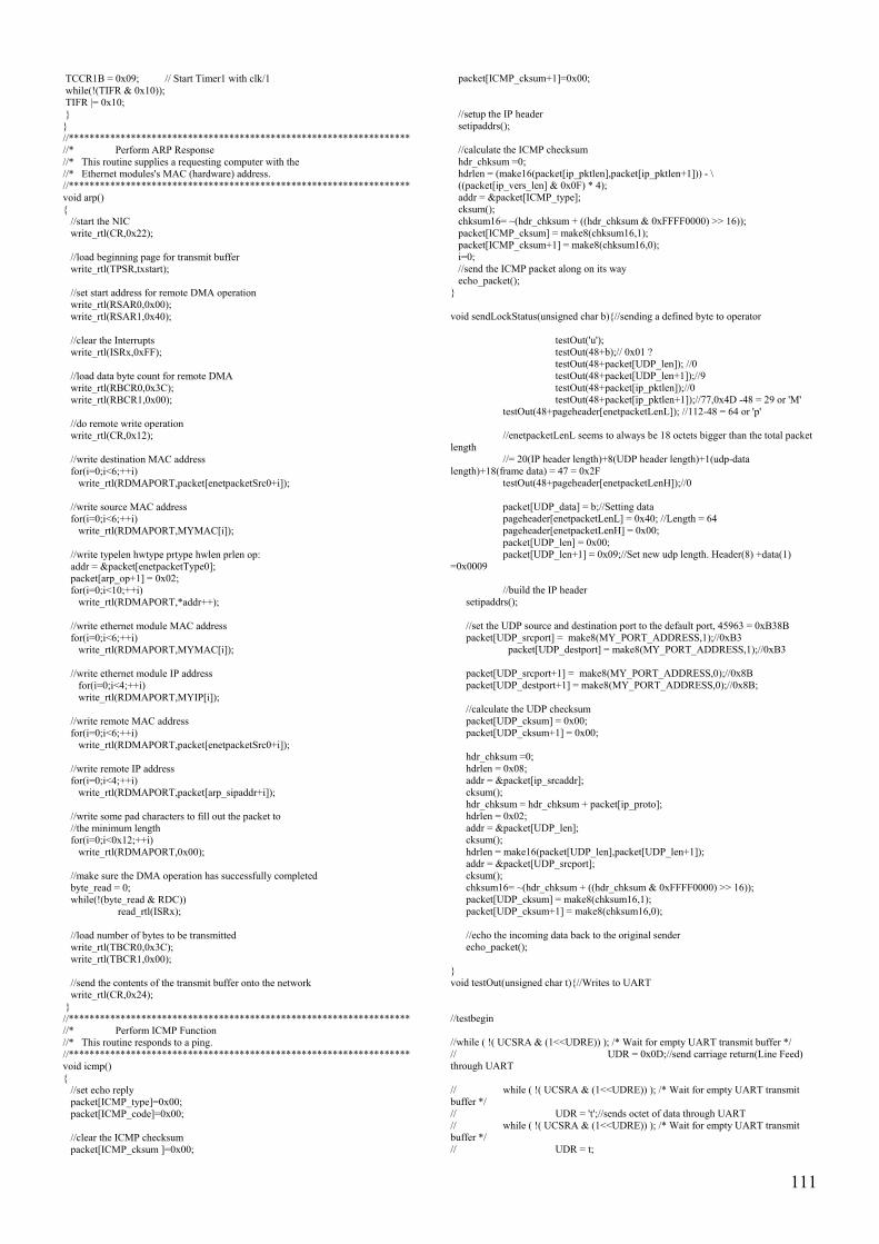
111
TCCR1B = 0x09; // Start Timer1 with clk/1 while(!(TIFR & 0x10)); TIFR |= 0x10; //****************************************************************** //* Perform ARP Response //* This routine supplies a requesting computer with the //* Ethernet modules's MAC (hardware) address. //****************************************************************** void arp() //start the NIC write_rtl(CR,0x22); //load beginning page for transmit buffer write_rtl(TPSR,txstart); //set start address for remote DMA operation write_rtl(RSAR0,0x00); write_rtl(RSAR1,0x40); //clear the Interrupts write_rtl(ISRx,0xFF); //load data byte count for remote DMA write_rtl(RBCR0,0x3C); write_rtl(RBCR1,0x00); //do remote write operation write_rtl(CR,0x12); //write destination MAC address for(i=0;i<6;++i) write_rtl(RDMAPORT,packet[enetpacketSrc0+i]); //write source MAC address for(i=0;i<6;++i) write_rtl(RDMAPORT,MYMAC[i]); //write typelen hwtype prtype hwlen prlen op: addr = &packet[enetpacketType0]; packet[arp_op+1] = 0x02; for(i=0;i<10;++i) write_rtl(RDMAPORT,*addr++); //write ethernet module MAC address for(i=0;i<6;++i) write_rtl(RDMAPORT,MYMAC[i]); //write ethernet module IP address for(i=0;i<4;++i) write_rtl(RDMAPORT,MYIP[i]); //write remote MAC address for(i=0;i<6;++i) write_rtl(RDMAPORT,packet[enetpacketSrc0+i]); //write remote IP address for(i=0;i<4;++i) write_rtl(RDMAPORT,packet[arp_sipaddr+i]); //write some pad characters to fill out the packet to //the minimum length for(i=0;i<0x12;++i) write_rtl(RDMAPORT,0x00); //make sure the DMA operation has successfully completed byte_read = 0; while(!(byte_read & RDC)) read_rtl(ISRx); //load number of bytes to be transmitted write_rtl(TBCR0,0x3C); write_rtl(TBCR1,0x00); //send the contents of the transmit buffer onto the network write_rtl(CR,0x24); //****************************************************************** //* Perform ICMP Function //* This routine responds to a ping. //****************************************************************** void icmp() //set echo reply packet[ICMP_type]=0x00; packet[ICMP_code]=0x00; //clear the ICMP checksum packet[ICMP_cksum ]=0x00;
packet[ICMP_cksum+1]=0x00; //setup the IP header setipaddrs(); //calculate the ICMP checksum hdr_chksum =0; hdrlen = (make16(packet[ip_pktlen],packet[ip_pktlen+1])) - \ ((packet[ip_vers_len] & 0x0F) * 4); addr = &packet[ICMP_type]; cksum(); chksum16= ~(hdr_chksum + ((hdr_chksum & 0xFFFF0000) >> 16)); packet[ICMP_cksum] = make8(chksum16,1); packet[ICMP_cksum+1] = make8(chksum16,0); i=0; //send the ICMP packet along on its way echo_packet(); void sendLockStatus(unsigned char b)//sending a defined byte to operator testOut('u'); testOut(48+b);// 0x01 ? testOut(48+packet[UDP_len]); //0 testOut(48+packet[UDP_len+1]);//9 testOut(48+packet[ip_pktlen]);//0 testOut(48+packet[ip_pktlen+1]);//77,0x4D -48 = 29 or 'M' testOut(48+pageheader[enetpacketLenL]); //112-48 = 64 or 'p' //enetpacketLenL seems to always be 18 octets bigger than the total packet length //= 20(IP header length)+8(UDP header length)+1(udp-data length)+18(frame data) = 47 = 0x2F testOut(48+pageheader[enetpacketLenH]);//0 packet[UDP_data] = b;//Setting data pageheader[enetpacketLenL] = 0x40; //Length = 64 pageheader[enetpacketLenH] = 0x00; packet[UDP_len] = 0x00; packet[UDP_len+1] = 0x09;//Set new udp length. Header(8) +data(1) =0x0009 //build the IP header setipaddrs(); //set the UDP source and destination port to the default port, 45963 = 0xB38B packet[UDP_srcport] = make8(MY_PORT_ADDRESS,1);//0xB3 packet[UDP_destport] = make8(MY_PORT_ADDRESS,1);//0xB3 packet[UDP_srcport+1] = make8(MY_PORT_ADDRESS,0);//0x8B packet[UDP_destport+1] = make8(MY_PORT_ADDRESS,0);//0x8B; //calculate the UDP checksum packet[UDP_cksum] = 0x00; packet[UDP_cksum+1] = 0x00; hdr_chksum =0; hdrlen = 0x08; addr = &packet[ip_srcaddr]; cksum(); hdr_chksum = hdr_chksum + packet[ip_proto]; hdrlen = 0x02; addr = &packet[UDP_len]; cksum(); hdrlen = make16(packet[UDP_len],packet[UDP_len+1]); addr = &packet[UDP_srcport]; cksum(); chksum16= ~(hdr_chksum + ((hdr_chksum & 0xFFFF0000) >> 16)); packet[UDP_cksum] = make8(chksum16,1); packet[UDP_cksum+1] = make8(chksum16,0); //echo the incoming data back to the original sender echo_packet(); void testOut(unsigned char t)//Writes to UART //testbegin //while ( !( UCSRA & (1<<UDRE)) ); /* Wait for empty UART transmit buffer */ // UDR = 0x0D;//send carriage return(Line Feed) through UART // while ( !( UCSRA & (1<<UDRE)) ); /* Wait for empty UART transmit buffer */ // UDR = 't';//sends octet of data through UART // while ( !( UCSRA & (1<<UDRE)) ); /* Wait for empty UART transmit buffer */ // UDR = t;

112
// UDR = pageheader[enetpacketLenH];//sends octet of data through UART // while ( !( UCSRA & (1<<UDRE)) ); /* Wait for empty UART transmit buffer */ // UDR = 't';//sends octet of data through UART // bin2hex(pageheader[enetpacketLenH]); // while ( !( UCSRA & (1<<UDRE)) ); /* Wait for empty UART transmit buffer */ // UDR = high_char;//sends octet of data through UART // while ( !( UCSRA & (1<<UDRE)) ); /* Wait for empty UART transmit buffer */ // UDR = low_char;//sends octet of data through UART //bin2hex(pageheader[enetpacketLenL]); // while ( !( UCSRA & (1<<UDRE)) ); /* Wait for empty UART transmit buffer */ // UDR = high_char;//sends octet of data through UART // while ( !( UCSRA & (1<<UDRE)) ); /* Wait for empty UART transmit buffer */ // UDR = low_char;//sends octet of data through UART // while ( !( UCSRA & (1<<UDRE)) ); /* Wait for empty UART transmit buffer */ // UDR = 0x0D;//send carriage return through UART //testend //****************************************************************** //* UDP Function //* This function uses UDP-packets from MyDDE Client 1.05 to receive data to control the radio and rig. //* It also echoes packets sent to port 7. //****************************************************************** void udp() //port 7 is the well-known echo port... echo that.. if(packet[UDP_destport] == 0x00 && packet[UDP_destport+1] ==0x07) //build the IP header setipaddrs(); //swap the UDP source and destination ports data_L = packet[UDP_srcport]; packet[UDP_srcport] = packet[UDP_destport]; packet[UDP_destport] = data_L; data_L = packet[UDP_srcport+1]; packet[UDP_srcport+1] = packet[UDP_destport+1]; packet[UDP_destport+1] = data_L; //calculate the UDP checksum packet[UDP_cksum] = 0x00; packet[UDP_cksum+1] = 0x00; hdr_chksum =0; hdrlen = 0x08; addr = &packet[ip_srcaddr]; cksum(); hdr_chksum = hdr_chksum + packet[ip_proto]; hdrlen = 0x02; addr = &packet[UDP_len]; cksum(); hdrlen = make16(packet[UDP_len],packet[UDP_len+1]); addr = &packet[UDP_srcport]; cksum(); chksum16= ~(hdr_chksum + ((hdr_chksum & 0xFFFF0000) >> 16)); packet[UDP_cksum] = make8(chksum16,1); packet[UDP_cksum+1] = make8(chksum16,0); //echo the incoming data back to the original sender echo_packet(); //UDP datagrams sent towards port address 45963 decimal (0xB38B) is decoded here. This data is output //to the rotor controller through the UART. else if(packet[UDP_destport] == 0xB3 && packet[UDP_destport+1] == 0x8B) unsigned char j = make16(packet[UDP_len],packet[UDP_len+1]) - 0x08;//Datagram length if(j == 0x01)//Command request switch (packet[UDP_data]) case 0x00: if(lockStatus == 0x00) sendLockStatus(0x00);//-----send status udp testOut('s'); else if(lockStatus == 0x01&& //If locked and incoming packet is from locked user, send LockedToRequestingIP(operational)(0x01)
lockedIP[0] == packet[ip_srcaddr] && lockedIP[1] == packet[ip_srcaddr+1] && lockedIP[2] == packet[ip_srcaddr+2] && lockedIP[3] == packet[ip_srcaddr+3] ) testOut('S'); sendLockStatus(0x01);//-----Send Status udp else if(lockStatus == 0x01)//locked, and not to calling IP sendLockStatus(0x0E);//-----Send LockedToOtherIP(busy)(0x0E) testOut('E'); break; case 0x01://Lock Command if(lockStatus == 0x00) //If on Standby, lock the incoming IP lockStatus = 0x01; lockedIP[0] = packet[ip_srcaddr]; lockedIP[1] = packet[ip_srcaddr+1]; lockedIP[2] = packet[ip_srcaddr+2]; lockedIP[3] = packet[ip_srcaddr+3]; testOut('L'); sendLockStatus(0x01);//------send Status udp else if((lockStatus == 0x01) && ( //If locked and lock command is NOT from locked user. !(lockedIP[0] == packet[ip_srcaddr]) || !(lockedIP[1] == packet[ip_srcaddr+1]) || !(lockedIP[2] == packet[ip_srcaddr+2]) || !(lockedIP[3] == packet[ip_srcaddr+3]))) testOut('N'); sendLockStatus(0x0E);//Send request denied(0x0E) break; case 0x02://Release Command if(lockStatus == 0x01 && //If locked and incoming packet is from locked user, release IP-lock lockedIP[0] == packet[ip_srcaddr] && lockedIP[1] == packet[ip_srcaddr+1] && lockedIP[2] == packet[ip_srcaddr+2] && lockedIP[3] == packet[ip_srcaddr+3] ) lockStatus = 0x00; testOut('O'); sendLockStatus(0x00);//Send Status udp break; // default: //end switch else if(j > 0x01)//Prosess UDP-data if(lockStatus == 0x00) //If on Standby, lock the incoming IP and process lockStatus = 0x01; lockedIP[0] = packet[ip_srcaddr]; lockedIP[1] = packet[ip_srcaddr+1]; lockedIP[2] = packet[ip_srcaddr+2]; lockedIP[3] = packet[ip_srcaddr+3]; testOut('l'); udpProcess(j); sendLockStatus(0x01);//------send Status udp else if(lockStatus == 0x01 && //If locked and incoming packet is from locked user, then process data, else drop packet lockedIP[0] == packet[ip_srcaddr] && lockedIP[1] == packet[ip_srcaddr+1] && lockedIP[2] == packet[ip_srcaddr+2] &&

113
lockedIP[3] == packet[ip_srcaddr+3] ) testOut('L'); udpProcess(j); else//Packet dropped testOut('N'); //End Size-if /* //LCD UDP application code else if(packet[UDP_destport] == 0x13 && packet[UDP_destport+1] == 0x88) switch (packet[UDP_data]) case 0: lcdcls; break; case 1: line1; break; case 2: line2; break; case 3: line3; break; case 4: line4; break; default: lcd_send_byte(1,packet[UDP_data]); */ /* ****************************************************************** * UDP Data processing block * Outputs udp-data to UART(rotor and radio) ****************************************************************** */ void udpProcess(unsigned char j)//j = length of UDP-data area unsigned char i; if(j>0x08) //both rotor and radio data in datafield for (i = 0; i <= 0x07; ++i) //looping through the assumed octets of data destined for the rotor in the UDP data field while ( !( UCSRA & (1<<UDRE)) ); /* Wait for empty UART transmit buffer */ UDR = packet[UDP_data+i];//sends octet of data through UART //end for-loop while ( !( UCSRA & (1<<UDRE)) ); /* Wait for empty UART transmit buffer */ UDR = 0x0D;//send carriage return through UART (for rotor acceptance) for (i = 0x08; i <= j; ++i) //looping through the rest of the data in the UDP data field("radio data") while ( !( UCSRA & (1<<UDRE)) ); /* Wait for empty UART transmit buffer */ UDR = packet[UDP_data+i];//sends octet of data through UART //end for-loop while ( !( UCSRA & (1<<UDRE)) ); /* Wait for empty UART transmit buffer */ UDR = 0x0D;//send carriage return through UART (so the rotor will look away from the last "nonsense") else if(j > 0x01)//only rotor data available. If the data-area is emty, only a line end is sent for (i = 0; i <= j; ++i) //looping through the assumed octets of data in the UDP data field while ( !( UCSRA & (1<<UDRE)) ); /* Wait for empty UART transmit buffer */ UDR = packet[UDP_data+i];//sends octet of data through UART //end for-loop. while ( !( UCSRA & (1<<UDRE)) ); /* Wait for empty UART transmit buffer */ UDR = 0x0D;//send carriage return through UART (for rotor)
// while ( !( UCSRA & (1<<UDRE)) ); /* Wait for empty UART transmit buffer */ // UDR = 0x0A;//send line feed through UART //****************************************************************** //* TCP Function //* This function uses TCP protocol to act as a Telnet server on //* port 8088 decimal. The application function is called with //* every incoming character. //****************************************************************** void tcp() int i,j; //assemble the destination port address from the incoming packet portaddr = make16(packet[TCP_destport],packet[TCP_destport+1]); //calculate the length of the data coming in with the packet //tcpdatalen_in = incoming packet length - incoming ip header length - //incoming tcp header length tcpdatalen_in = (make16(packet[ip_pktlen],packet[ip_pktlen+1]))- \ ((packet[ip_vers_len] & 0x0F)* 4)-(((packet[TCP_hdrflags] & 0xF0) >> 4) * 4); //If an ACK is received and the destination port address is valid //and no data is in the packet if(ACK_IN && portaddr == MY_PORT_ADDRESS && tcpdatalen_in == 0x00) //assemble the acknowledgment number from the incoming packet incoming_ack =make32(packet[TCP_acknum],packet[TCP_acknum+1], \ packet[TCP_acknum+2],packet[TCP_acknum+3]); //if the incoming packet is a result of session establishment if(synflag_bit) //clear the SYN flag clr_synflag; //the incoming acknowledgment is my new sequence number my_seqnum = incoming_ack; //send the Telnet server banner //limit the character count to 40 decimal j = sizeof(telnet_banner); for(i=0;i<j;++i) packet[TCP_data+i] = telnet_banner[i]; //length of the banner message tcpdatalen_out = j; //send the Telnet server banner //limit the character count to 40 decimal //strcpy(&packet[TCP_data],"EDTP AVR Telnet SERVER>"); //length of the banner message //tcpdatalen_out = 23; //expect to get an acknowledgment of the banner message expected_ack = my_seqnum +tcpdatalen_out; //send the TCP/IP packet send_tcp_packet(); //if an ack is received and the port address is valid and there is data //in the incoming packet if((ACK_IN) && portaddr == MY_PORT_ADDRESS && tcpdatalen_in) for(i=0;i<tcpdatalen_in;++i) //receive the data and put it into the incoming data buffer aux_data[i] = packet[TCP_data+i]; application_code(); //assemble the acknowledgment number from the incoming packet incoming_ack =make32(packet[TCP_acknum],packet[TCP_acknum+1], \ packet[TCP_acknum+2],packet[TCP_acknum+3]); //check for the number of bytes acknowledged //determine how many bytes are outstanding and adjust the outgoing //sequence number accordingly if(incoming_ack <= expected_ack) my_seqnum = expected_ack - (expected_ack - incoming_ack); //my expected acknowledgement number expected_ack = my_seqnum +tcpdatalen_out; send_tcp_packet();

114
//this code segment processes the incoming SYN from the Telnet client //and sends back the initial sequence number (ISN) and acknowledges //the incoming SYN packet if(SYN_IN && portaddr == MY_PORT_ADDRESS) tcpdatalen_in = 0x01; set_synflag; setipaddrs(); data_L = packet[TCP_srcport]; packet[TCP_srcport] = packet[TCP_destport]; packet[TCP_destport] = data_L; data_L = packet[TCP_srcport+1]; packet[TCP_srcport+1] = packet[TCP_destport+1]; packet[TCP_destport+1] = data_L; assemble_ack(); if(++ISN == 0x0000 || ++ISN == 0xFFFF) my_seqnum = 0x1234FFFF; set_packet32(TCP_seqnum,my_seqnum); packet[TCP_hdrflags+1] = 0x00; SYN_OUT; ACK_OUT; packet[TCP_cksum] = 0x00; packet[TCP_cksum+1] = 0x00; hdr_chksum =0; hdrlen = 0x08; addr = &packet[ip_srcaddr]; cksum(); hdr_chksum = hdr_chksum + packet[ip_proto]; tcplen = make16(packet[ip_pktlen],packet[ip_pktlen+1]) - \ ((packet[ip_vers_len] & 0x0F) * 4); hdr_chksum = hdr_chksum + tcplen; hdrlen = tcplen; addr = &packet[TCP_srcport]; cksum(); chksum16= ~(hdr_chksum + ((hdr_chksum & 0xFFFF0000) >> 16)); packet[TCP_cksum] = make8(chksum16,1); packet[TCP_cksum+1] = make8(chksum16,0); echo_packet(); //this code segment processes a FIN from the Telnet client //and acknowledges the FIN and any incoming data. if(FIN_IN && portaddr == MY_PORT_ADDRESS) if(tcpdatalen_in) for(i=0;i<tcpdatalen_in;++i) aux_data[i] = packet[TCP_data+i]; application_code(); set_finflag; ++tcpdatalen_in; incoming_ack =make32(packet[TCP_acknum],packet[TCP_acknum+1], \ packet[TCP_acknum+2],packet[TCP_acknum+3]); if(incoming_ack <= expected_ack) my_seqnum = expected_ack - (expected_ack - incoming_ack); expected_ack = my_seqnum +tcpdatalen_out; send_tcp_packet(); //****************************************************************** //* Assemble the Acknowledgment //* This function assembles the acknowledgment to send to //* to the client by adding the received data count to the //* client's incoming sequence number. //****************************************************************** void assemble_ack() client_seqnum=make32(packet[TCP_seqnum],packet[TCP_seqnum+1], \ packet[TCP_seqnum+2],packet[TCP_seqnum+3]); client_seqnum = client_seqnum + tcpdatalen_in; set_packet32(TCP_acknum,client_seqnum); //****************************************************************** //* Send TCP Packet
//* This routine assembles and sends a complete TCP/IP packet. //* 40 bytes of IP and TCP header data is assumed. //****************************************************************** void send_tcp_packet() //count IP and TCP header bytes.. Total = 40 bytes ip_packet_len = 40 + tcpdatalen_out; packet[ip_pktlen] = make8(ip_packet_len,1); packet[ip_pktlen+1] = make8(ip_packet_len,0); setipaddrs(); data_L = packet[TCP_srcport]; packet[TCP_srcport] = packet[TCP_destport]; packet[TCP_destport] = data_L; data_L = packet[TCP_srcport+1]; packet[TCP_srcport+1] = packet[TCP_destport+1]; packet[TCP_destport+1] = data_L; assemble_ack(); set_packet32(TCP_seqnum,my_seqnum); packet[TCP_hdrflags+1] = 0x00; ACK_OUT; if(flags & finflag) FIN_OUT; clr_finflag; packet[TCP_cksum] = 0x00; packet[TCP_cksum+1] = 0x00; hdr_chksum =0; hdrlen = 0x08; addr = &packet[ip_srcaddr]; cksum(); hdr_chksum = hdr_chksum + packet[ip_proto]; tcplen = ip_packet_len - ((packet[ip_vers_len] & 0x0F) * 4); hdr_chksum = hdr_chksum + tcplen; hdrlen = tcplen; addr = &packet[TCP_srcport]; cksum(); chksum16= ~(hdr_chksum + ((hdr_chksum & 0xFFFF0000) >> 16)); packet[TCP_cksum] = make8(chksum16,1); packet[TCP_cksum+1] = make8(chksum16,0); txlen = ip_packet_len + 14; if(txlen < 60) txlen = 60; data_L = make8(txlen,0); data_H = make8(txlen,1); write_rtl(CR,0x22); write_rtl(TPSR,txstart); write_rtl(RSAR0,0x00); write_rtl(RSAR1,0x40); write_rtl(ISRx,0xFF); write_rtl(RBCR0,data_L); write_rtl(RBCR1,data_H); write_rtl(CR,0x12); for(i=0;i<txlen;++i) write_rtl(RDMAPORT,packet[enetpacketDest0+i]); byte_read = 0; while(!(byte_read & RDC)) read_rtl(ISRx); write_rtl(TBCR0,data_L); write_rtl(TBCR1,data_H); write_rtl(CR,0x24); //****************************************************************** //* Read/Write for show_regs //* This routine reads a NIC register and dumps it out to the //* serial port as ASCII. //****************************************************************** void readwrite() read_rtl(i); bin2hex(byte_read); printf("\t%c%c",high_char,low_char); //****************************************************************** //* Displays Control Registers in Pages 1, 2 and 3 //* This routine dumps all of the NIC internal registers //* to the serial port as ASCII characters. //****************************************************************** void show_regs() write_rtl(CR,0x21);

115
cls(); printf("\r\n"); printf(" Realtek 8019AS Register Dump\n\n\r"); printf("REG\tPage0\tPage1\tPage2\tPage3\n\r"); for(i=0;i<16;++i) bin2hex((unsigned char) i); printf("%c%c",high_char,low_char); write_rtl(CR,0x21); readwrite(); write_rtl(CR,0x61); readwrite(); write_rtl(CR,0xA1); readwrite(); write_rtl(CR,0xE1); readwrite(); printf("\r\n"); //****************************************************************** //* Dump Receive Ring Buffer Header //* This routine dumps the 4-byte receive buffer ring header //* to the serial port as ASCII characters. //****************************************************************** void dump_header() for(i=0;i<4;++i) bin2hex(pageheader[i]); printf("\r\n%c%c",high_char,low_char); //****************************************************************** //* Converts Binary to Displayable Hex Characters //* ie.. 0x00 in gives 0x30 and 0x30 out //****************************************************************** void bin2hex(unsigned char binchar) high_nibble = (binchar & 0xF0) / 16; if(high_nibble > 0x09) high_char = high_nibble + 0x37; else high_char = high_nibble + 0x30; low_nibble = (binchar & 0x0F); if(low_nibble > 0x09) low_char = low_nibble + 0x37; else low_char = low_nibble + 0x30; //****************************************************************** //* Used with Tera Term to clear the screen (VT-100 command) //****************************************************************** void cls(void) printf("%c[2J",esc); //****************************************************************** //* show_packet //* This routine is for diagnostic purposes and displays //* the Packet Buffer memory in the AVR. //****************************************************************** void show_packet() cls(); printf("\r\n"); data_L = 0x00; for(i=0;i<96;++i) bin2hex(packet[i]); printf(" %c%c",high_char,low_char); if(++data_L == 0x10) data_L = 0x00; printf("\r\n"); //****************************************************************** //* show_aux_packet //* This routine is a diagnostic that displays Auxillary //* Packet Buffer buffer memory in the AVR. //****************************************************************** void show_aux_packet() cls(); printf("\r\n"); data_L = 0x00; for(i=0;i<80;++i)
bin2hex(aux_data[i]); printf(" %c%c",high_char,low_char); if(++data_L == 0x10) data_L = 0x00; printf("\r\n"); //****************************************************************** //* Write to NIC Control Register //****************************************************************** void write_rtl(unsigned int regaddr, unsigned int regdata) rtladdr = regaddr; rtldata = regdata; tortl; nop; clr_iow_pin; nop; set_iow_pin; nop; fromrtl; rtldata = 0xFF; //****************************************************************** //* Read From NIC Control Register //****************************************************************** void read_rtl(unsigned int regaddr) fromrtl; rtldata = 0xFF; rtladdr = regaddr; clr_ior_pin; nop; byte_read = PINA; nop; set_ior_pin; nop; //****************************************************************** //* Handle Receive Ring Buffer Overrun //* No packets are recovered //****************************************************************** void overrun() read_rtl(CR); data_L = byte_read; write_rtl(CR,0x21); delay_ms(2); write_rtl(RBCR0,0x00); write_rtl(RBCR1,0x00); if(!(data_L & 0x04)) resend = 0; else if(data_L & 0x04) read_rtl(ISRx); data_L = byte_read; if((data_L & 0x02) || (data_L & 0x08)) resend = 0; else resend = 1; write_rtl(TCR,0x02); write_rtl(CR,0x22); write_rtl(BNRY,rxstart); write_rtl(CR,0x62); write_rtl(CURR,rxstart); write_rtl(CR,0x22); write_rtl(ISRx,0x10); write_rtl(TCR,tcrval); //****************************************************************** //* Echo Packet Function //* This routine does not modify the incoming packet size and //* thus echoes the original packet structure. //****************************************************************** void echo_packet() write_rtl(CR,0x22); write_rtl(TPSR,txstart); write_rtl(RSAR0,0x00); write_rtl(RSAR1,0x40); write_rtl(ISRx,0xFF); write_rtl(RBCR0,pageheader[enetpacketLenL] - 4 ); write_rtl(RBCR1,pageheader[enetpacketLenH]); write_rtl(CR,0x12); txlen = make16(pageheader[enetpacketLenH],pageheader[enetpacketLenL]) - 4;

116
for(i=0;i<txlen;++i) write_rtl(RDMAPORT,packet[enetpacketDest0+i]); byte_read = 0; while(!(byte_read & RDC)) read_rtl(ISRx); write_rtl(TBCR0,pageheader[enetpacketLenL] - 4); write_rtl(TBCR1,pageheader[enetpacketLenH]); write_rtl(CR,0x24); //****************************************************************** //* Get A Packet From the Ring //* This routine removes a data packet from the receive buffer //* ring. //****************************************************************** void get_frame() //execute Send Packet command to retrieve the packet write_rtl(CR,0x1A); for(i=0;i<4;++i) read_rtl(RDMAPORT); pageheader[i] = byte_read; rxlen = make16(pageheader[enetpacketLenH],pageheader[enetpacketLenL]); for(i=0;i<rxlen;++i) read_rtl(RDMAPORT); //dump any bytes that will overrun the receive buffer if(i < 96) packet[i] = byte_read; while(!(byte_read & RDC)) read_rtl(ISRx); write_rtl(ISRx,0xFF); //process an ARP packet if(packet[enetpacketType0] == 0x08 && packet[enetpacketType1] == 0x06) if(packet[arp_hwtype+1] == 0x01 && packet[arp_prtype] == 0x08 && packet[arp_prtype+1] == 0x00 && packet[arp_hwlen] == 0x06 && packet[arp_prlen] == 0x04 && packet[arp_op+1] == 0x01 && MYIP[0] == packet[arp_tipaddr] && MYIP[1] == packet[arp_tipaddr+1] && MYIP[2] == packet[arp_tipaddr+2] && MYIP[3] == packet[arp_tipaddr+3] ) arp(); //process an IP packet else if(packet[enetpacketType0] == 0x08 && packet[enetpacketType1] == 0x00 && packet[ip_destaddr] == MYIP[0] && packet[ip_destaddr+1] == MYIP[1] && packet[ip_destaddr+2] == MYIP[2] && packet[ip_destaddr+3] == MYIP[3]) if(packet[ip_proto] == PROT_ICMP) icmp(); else if(packet[ip_proto] == PROT_UDP) udp(); else if(packet[ip_proto] == PROT_TCP) tcp(); //****************************************************************** //* SETIPADDRS //* This function builds the IP header. //****************************************************************** void setipaddrs() //move IP source address to destination address packet[ip_destaddr]=packet[ip_srcaddr]; packet[ip_destaddr+1]=packet[ip_srcaddr+1]; packet[ip_destaddr+2]=packet[ip_srcaddr+2]; packet[ip_destaddr+3]=packet[ip_srcaddr+3]; //make ethernet module IP address source address packet[ip_srcaddr]=MYIP[0]; packet[ip_srcaddr+1]=MYIP[1]; packet[ip_srcaddr+2]=MYIP[2]; packet[ip_srcaddr+3]=MYIP[3]; //move hardware source address to destination address packet[enetpacketDest0]=packet[enetpacketSrc0]; packet[enetpacketDest1]=packet[enetpacketSrc1]; packet[enetpacketDest2]=packet[enetpacketSrc2]; packet[enetpacketDest3]=packet[enetpacketSrc3]; packet[enetpacketDest4]=packet[enetpacketSrc4]; packet[enetpacketDest5]=packet[enetpacketSrc5];
//make ethernet module mac address the source address packet[enetpacketSrc0]=MYMAC[0]; packet[enetpacketSrc1]=MYMAC[1]; packet[enetpacketSrc2]=MYMAC[2]; packet[enetpacketSrc3]=MYMAC[3]; packet[enetpacketSrc4]=MYMAC[4]; packet[enetpacketSrc5]=MYMAC[5]; //calculate the IP header checksum packet[ip_hdr_cksum]=0x00; packet[ip_hdr_cksum+1]=0x00; hdr_chksum =0; hdrlen = (packet[ip_vers_len] & 0x0F) * 4; addr = &packet[ip_vers_len]; cksum(); chksum16= ~(hdr_chksum + ((hdr_chksum & 0xFFFF0000) >> 16)); packet[ip_hdr_cksum] = make8(chksum16,1); packet[ip_hdr_cksum+1] = make8(chksum16,0); //****************************************************************** //* CHECKSUM CALCULATION ROUTINE //****************************************************************** void cksum() while(hdrlen > 1) data_H=*addr++; data_L=*addr++; chksum16=make16(data_H,data_L); hdr_chksum = hdr_chksum + chksum16; hdrlen -=2; if(hdrlen > 0) data_H=*addr; data_L=0x00; chksum16=make16(data_H,data_L); hdr_chksum = hdr_chksum + chksum16; //****************************************************************** //* Initialize the RTL8019AS //****************************************************************** void init_RTL8019AS() fromrtl; // PORTA data lines = input rtldata = 0xFF; DDRB = 0xFF; rtladdr = 0x00; // clear address lines DDRC = 0xFF; DDRD = 0xFA; // setup IOWB, IORB, EEPROM,RXD,TXD,CTS,LE PORTD = 0x05; // enable pullups on input pins // clr_le_pin; //initialize latch enable for HCT573 //Not needed clr_EEDO; set_iow_pin; // disable IOWB set_ior_pin; // disable IORB set_rst_pin; // put NIC in reset delay_ms(2); // delay at least 1.6ms clr_rst_pin; // disable reset line read_rtl(RSTPORT); // read contents of reset port write_rtl(RSTPORT,byte_read); // do soft reset delay_ms(10); // give it time read_rtl(ISRx); // check for good soft reset if(!(byte_read & RST)) while(1) printf("RTL8019AS INIT FAILED!\r\n"); delay_ms(1000); write_rtl(CR,0x21); // stop the NIC, abort DMA, page 0 delay_ms(2); // make sure nothing is coming in or going out write_rtl(DCR,dcrval); // 0x58 write_rtl(RBCR0,0x00); write_rtl(RBCR1,0x00); write_rtl(RCR,0x04); write_rtl(TPSR,txstart); write_rtl(TCR,0x02); write_rtl(PSTART,rxstart); write_rtl(BNRY,rxstart); write_rtl(PSTOP,rxstop); write_rtl(CR,0x61); write_rtl(CURR,rxstart);

117
for(i=0;i<6;++i) write_rtl(PAR0+i, MYMAC[i]); write_rtl(CR,0x22); write_rtl(ISRx,0xFF); write_rtl(IMR,imrval); write_rtl(TCR,tcrval); //****************************************************************** //* MAIN MAIN MAIN MAIN MAIN MAIN MAIN MAIN MAIN MAIN MAIN MAIN //****************************************************************** //void C_task main(void) int main(void) //lcd_init(); init_RTL8019AS(); init_USART(b9600); // sets baudrate on UART and transmits enter-sign //init_PWM(); lockStatus = 0x00; clr_synflag; clr_finflag; //printf("Easy Ethernet W For AVR Version 03.08.19\r\n"); //****************************************************************** //* Look for a packet in the receive buffer ring //****************************************************************** while(1) //* Looking for a packet in the receive buffer ring //start the NIC write_rtl(CR,0x22); //wait for a good packet while(!(PIND & INT0_pin)); //read the interrupt status register read_rtl(ISRx); //if the receive buffer has been overrun if(byte_read & OVW) overrun(); //if the receive buffer holds a good packet if(byte_read & PRX) get_frame(); //make sure the receive buffer ring is empty //if BNRY = CURR, the buffer is empty read_rtl(BNRY); data_L = byte_read; write_rtl(CR,0x62); read_rtl(CURR); data_H = byte_read; write_rtl(CR,0x22); //buffer is not empty.. get next packet if(data_L != data_H) get_frame(); //reset the interrupt bits write_rtl(ISRx,0xFF); //* Stop Looking for a packet in the receive buffer ring //* Reset IC-910h(radio) control command test cycle /* if(LSB == 0) IC910_command(0x06,0x01,1,0,0); LSB = 1; else delay_ms(500); IC910_command(0x06,0x03,1,0,0); LSB = 0; */


Appendix F – Important Code snippets from MyDDE 1.50 Language: Object pascal See attached Delphi 7-project files for complete description Main.pas:
procedure TFMain.FormCreate(Sender: TObject); begin ParseString('',SatData); PrintData(SatData); PathP:=ExtractFileDir(ParamStr(0)); if PathP[length(PathP)]<>'\' then PathP:=PathP+'\'; ChDir(PathP); If not FileExists(PathP+'Orbitron.exe') then begin Reg:=TRegistry.Create; try if Reg.OpenKey('\Software\Stoff\Orbitron',True) then Tracking.ServiceApplication:=Reg.ReadString('Path')+'orbitron'; finally Reg.CloseKey; Reg.Free; end; end; Tracking.OpenLink; ComboBox1.Items.LoadFromFile('RemoteGroundStationList.cfg');//Loading IP:Port-addresses from file //RadioControl statics StartString:= Chr(254)+Chr(254)+Chr(96)+Chr(224); StopString:= Chr(253); SetFCmd:= Chr(6)+Chr(0); GetFCmd:= Chr(5)+Chr(0); Memo1.Lines.Add('LocalHostName ='+IdUDPServer1.LocalName); Memo1.Lines.Add('LocalHostAddress='+GStack.LocalAddress); Memo1.Lines.Add('Port = '+IntToStr(IdUDPServer1.DefaultPort)); Memo1.Lines.Add('BufferSize ='+IntToStr(IdUDPServer1.BufferSize)); Memo1.Lines.Add('LocalServerActive = '+BoolToStr(IdUDPServer1.Active,True)); IdUDPServer1.Active := True; end;
procedure TFMain.UpdateRotorAndRadio(data: TSatData); var Sazm, Selv : Double;//Corrected azimuth and elevation Sdnf, Supf : Double;//Corrected downlink and uplink frequency in kHz TmpAzm : Double; tmp : String; tmi : Integer; FreqBCD : String; RadioString : String; begin Please write support for your rotor/radio hardware here. Use DATA record as source of current tracking data sent by Orbitron. This procedure will be called by DDE engine after Orbitron made changes into the tracking data (each 1s, 5s, 10s or so). //Adding Corrections to Azimuth and Elevation if(TryStrToFloat(Edit2.Text,Sazm) and TryStrToFloat(Edit3.Text,Selv))//Corrections successfully converted to float then begin Sazm := Sazm+data.azm; //Corrected azimuth and elevation Selv := Selv+data.elv; end else begin
Edit1.Text := 'Edit2.float= '+Edit2.Text+'Conv: '+BoolToStr(TryStrToFloat(Edit2.Text,Sazm),TRUE);//test Sazm := data.azm; //Uncorrected azimuth and elevation to be sent over IP Selv := data.elv; //ShowMessage('Azimuth and elevation correction boxes must be in float format("-12.5")'); end; if (CheckBox2.Checked and (Selv<StrToFloat(Edit6.Text))) then begin//Deactivating rig and driver if satellite is below set horizon(elevation) limit Selv := 0; Sazm := 0; Sdnf := 0; Supf := 0; if(RigLock = 1) then begin IdUDPServer1.Send(TargetIPAddress,TargetPort,'W'+FormatFloat('000',Sazm)+' '+FormatFloat('000',Selv));//Resetting antenna-position IdUDPServer1.Send(TargetIPAddress,TargetPort,Chr(2));//releasing lock on rig-controller end; if(DriverActive = True) then begin DriverActive := False; Label28.Caption := 'Driver inactive'; Label28.Color := clGreen; end; end else if(RigLock <> 14) then begin //Unless rig is busy.. if((RigLock = 0) and (IdUDPServer1.Active = True)) then begin //"lock and load" Memo1.Lines.Add('Selv deactivation bool:'+BoolToStr((Selv<StrToFloat(Edit6.Text)),TRUE)); Memo1.Lines.Add('Selv:'+FloatToStr(Selv)+'Edit6:'+FloatToStr(StrToFloat(Edit6.Text))); IdUDPServer1.Send(TargetIPAddress,TargetPort,Chr(1));//Request rig-lock. Memo1.Lines.Add('Sending reqRigLock 0x01'); end; DriverActive := True; Label28.Caption := 'Driver active'; Label28.Color := clRed; TmpAzm:= 0; if(not AnsiSameText(Lastdnm,data.dnm)) then begin //Downlink mode change detected tmp := Chr($0d); if(AnsiSameText(data.dnm,'LSB')) then begin IdUDPServer1.Send(TargetIPAddress,TargetPort,tmp+tmp+tmp+tmp+tmp+tmp+tmp+tmp+StartString+SetFCmd+Chr($01)+StopString); Memo1.Lines.Add('Sending radio mode change'); Label24.Caption := 'LSB'; end; if(AnsiSameText(data.dnm,'USB')) then begin IdUDPServer1.Send(TargetIPAddress,TargetPort,tmp+tmp+tmp+tmp+tmp+tmp+tmp+tmp+StartString+SetFCmd+Chr($02)+StopString); Label24.Caption := 'USB'; Memo1.Lines.Add('Sending radio mode change'); end; if(AnsiSameText(data.dnm,'FM')) then begin IdUDPServer1.Send(TargetIPAddress,TargetPort,tmp+tmp+tmp+tmp+tmp+tmp+tmp+tmp+StartString+Chr($07)+StopString); Label24.Caption := 'FM'; Memo1.Lines.Add('Sending radio mode change'); end; if(AnsiSameText(data.dnm,'FM-N')) then begin IdUDPServer1.Send(TargetIPAddress,TargetPort,tmp+tmp+tmp+tmp+tmp+tmp+tmp+tmp+StartString+Chr($07)+StopString);

120
Label24.Caption := 'FM-N'; Memo1.Lines.Add('Sending radio mode change'); end; if(AnsiSameText(data.dnm,'CW') or AnsiSameText(data.dnm,'CW-N')) then begin IdUDPServer1.Send(TargetIPAddress,TargetPort,tmp+tmp+tmp+tmp+tmp+tmp+tmp+tmp+StartString+SetFCmd+Chr($04)+StopString); Memo1.Lines.Add('Sending radio mode change'); Label24.Caption := 'CW or CW-N'; if(Checkbox3.Checked) then begin Edit4.Text := '-2.0'; // ShowMessage('Downlink CW or CW-N mode has been detected. To be able to listen to baseband morse-code a -2kHz frequency correction has been entered'); end else Edit4.Text := '-0.0'; end else Edit4.Text := '-0.0'; end; if(not AnsiSameText(Lastupm,data.upm)) then begin //Uplink mode change detected if(AnsiSameText(data.upm,'CW') or AnsiSameText(data.upm,'CW-N')) then begin if(Checkbox3.Checked) then begin Edit5.Text := '-2.0'; // ShowMessage('Uplink CW or CW-N mode has been detected. To be able to transmit a baseband morse-code, a -2kHz frequency correction has been entered'); end else Edit5.Text := '-0.0'; end else Edit5.Text := '-0.0'; end; Lastdnm := data.dnm; Lastupm := data.upm; if(TryStrToFloat(Edit7.Text,TmpAzm))//Azimuth offset successfully converted to float then Sazm := Sazm+TmpAzm; //Offset-corrected azimuth to be sent over IP if(CheckBox1.Checked) then begin //Makes the antenna use the ekstra 90 degrees of azimuth movement(450 degree support) if((LastValidAzimuth>330) and (Sazm<90)) then Sazm := Sazm + 360;//If the satellite traverses 359->001 degrees azimuth, then use the 450 area. end; LastValidAzimuth := Sazm; if(TryStrToFloat(Edit4.Text,Sdnf) and TryStrToFloat(Edit5.Text,Supf)) then begin //Corrections successfully converted to float Sdnf := (Sdnf*1000) + data.dnf; //Corrected downlink and uplink frequency to be sent over IP Supf := (Supf*1000) + data.upf; end else begin Sdnf := data.dnf; //Uncorrected downlink and uplink frequency to be sent over IP Supf := data.upf; //ShowMessage('Downlink and uplink frequency correction boxes must be in float format("-12.5")'); end; if(Selv<0) then Selv := 0; //Do not transmit negative elevation as it is not supported if(ComboBox1.ItemIndex >0) then begin // Label26.Caption := 'Rig activated'; // Label26.Color := clRed;
Radio control Downlink frequency control tmi:= Round(data.dnf); FreqBCD:= Chr(((tmi Div 10)Mod 10)*16+((tmi Div 1)Mod 10)) +Chr(((tmi Div 1000)Mod 10)*16+((tmi Div 100)Mod 10)) +Chr(((tmi Div 100000)Mod 10)*16+((tmi Div 10000)Mod 10)) +Chr(((tmi Div 10000000)Mod 10)*16+((tmi Div 1000000)Mod 10)) +Chr((tmi Div 100000000)Mod 10); RadioString:= StartString+SetFCmd+FreqBCD+StopString; IdUDPServer1.Send(TargetIPAddress,TargetPort,'W'+FormatFloat('000',Sazm)+' '+FormatFloat('000',Selv)+RadioString); Memo1.Lines.Add('Sending Whhh hhh'); end; end; //end "deactivation-if" Label13.Caption := FormatFloat('000',Sazm); Label14.Caption := FormatFloat('000',Selv); Label18.Caption := FormatFloat('000" "000" "000',Sdnf)+' Hz'; Label19.Caption := FormatFloat('000" "000" "000',Supf)+' Hz'; end; procedure TFMain.IdUDPServer1UDPRead(Sender: TObject; AData: TStream; ABinding: TIdSocketHandle); var ReceivedData : TMemoryStream; Lockstatus : String; bu : Byte; begin ReceivedData := TMemoryStream.Create; ReceivedData.LoadFromStream(AData); ReceivedData.Read(bu,1); ReceivedData.Read(LockStatus,25); Memo1.Lines.Add('Received:'+IntToStr(Integer(bu))+Lockstatus+':'); //.ReadString(50); // if(bu = 0)then begin//AData.Size > 0) then begin // LockStatus := ;//LeftStr(bu,1); if(bu = 0) then begin // Memo1.Lines.Add('bu=0'); RigLock := 0; Label26.Caption := 'Rig status INACTIVE'; Label26.Color := clGreen; end else if(bu = 1) then begin // Memo1.Lines.Add('bu=1'); RigLock := 1; Label26.Caption := 'Rig status ACTIVATED'; Label26.Color := clRed; end else if(bu = 14) then begin // Memo1.Lines.Add('bu=14'); RigLock := 14; Label26.Caption := 'Rig status BUSY'; Label26.Color := clPurple; end; // end;
ReceivedData.Free(); end;

Appendix G - SP2000 & SP7000 Preamplifier Curvesxix
Low Noise GaAsFet Design using single gate selected microwave Fets Hi-Q Helical Coils & Helical Filters (SP-2000/7000) RF-Sensed (VOX) or PTT (Hard Keyed) operation Voltage Feed via coax or separate line. High Quality Coaxial Relays with N-type Connectors Two cabinet construction with shielded inner box Weatherproof Housin
MODEL FREQ. NF-MAX GAIN-Adj. Filters VOX/PTT SP-2000 144.0MHz. 0.8 approx. 10-20dB HELICAL 200/750 SP-7000 432/435MHz. 0.9 approx. 10-20dB HELICAL 100/500 SP2000 Series
Graph 1: This graph illustrates the SP-2000 preamplifier filter characteristics. Center frequency =
145.0MHz, SPAN = 100MHz, Vertical Marker Pointer = 22.062dB Gain. Horizontal Marker Pointer = 0.0dB Reference, 10dB per division
SP-7000 Series
Graph 2: This graph illustrates the SP-7000 preamplifier filter characteristics. Center frequency =
435.0MHz, SPAN = 100MHz, Vertical Marker Pointer = 20.22dB Gain. Horizontal Marker Pointer = 0.0dB Reference, 10dB per division


Appendix H – Important pages from ICOM 910h manual

124

125

126

127

128

Appendix I – Important pages of the
Yaesu RS-232B manual

130

Appendix J –Parts list of the Oslo Satellite ground station


i http://scienceworld.wolfram.com/physics/MaxwellEquations.html, 2009-10-15 ii http://scienceworld.wolfram.com/physics/MaxwellEquations.html, 2009-10-15 iii Tipler, Paul (2004). Physics for Scientists and Engineers: Electricity, Magnetism, Light, and Elementary Modern Physics (5th ed.). W. H. Freeman. ISBN 0-7167-0810-8. iv Golo, G. and Talasila, V. and Schaft van der, A.J. (2002) Approximation of the telegrapher's equations. In: 41st IEEE Conference on Decision and Control, 2002, Las Vegas, Nevada, U.S.A. v “Handbook of Linear Partial Differential Equations for Engineers and Scientists” by Andrei D. Polyanin, ISBN:9781584882992, pub. Nov 28, 2001. vi Wikipedia, http://en.wikipedia.org/wiki/Isotropic_radiator , 2009-11-18 vii http://en.wikipedia.org/wiki/File:Dipole_Antenna.jpg, 2009-11-19 viii NBS TECHNICAL NOTE 688 – Yagi Antenna Design, issued dec. 1976. http://tf.nist.gov/timefreq/general/pdf/451.pdf, 2009-11-28 ix The article “Why 50Ohms?”, http://www.microwaves101.com/encyclopedia/why50ohms.cfm, 2009-12-08 x http://sv1bsx.50webs.com/antenna-pol/polarization.html, 2009-11-16 xi W. L. Stutzman and G. A. Thiele, Antenna Theory and Design, John Wiley & Sons, New York, 1981. xii General Conference, Davos, 11 to 16 September 2005, Definition of Modes: NBFM, Paper number: 17, International Amateur Radio Union Region 1, http://www.rsgb-spectrumforum.org.uk/Papers/VHF/Davos%20C5%20Papers/DV05_C5_17%20SARL%20NBFM.pdf xiii Communication Theory, by T G Thomas S Chandra Sekhar. http://books.google.no/books?id=C1C6IBiCoXsC&lpg=PA238&ots=v2FG2n66zg&dq=FM%20threshold%20vs%20SNR&pg=PA238#v=onepage&q=&f=false page 238. ISBN 0070590915, 9780070590915, publisher: Tata McGraw-Hill, 2005 xiv Wikipedia, Non-return-to-zero, http://en.wikipedia.org/w/index.php?title=Non-return-to-zero&oldid=334853041 (last visited Jan. 11, 2010) xv APPLICATION NOTE, MX589 GMSK MODEM Application, MX589_GMSK_Application.pdf.. xvi THRESHOLD DETECTION PERFORMANCE OF GMSK SIGNAL WITH BT==O.5 by Gee L. Lui at The Aerospace Corporation, Communication Systems Engineering Department. El Segundo, California. http://www.argreenhouse.com/society/TacCom/papers98/15_02i.pdf xvii ICOM 910H service-manual, S-13714HZ-C1 © 2001 Icom Inc. Cut-out from page 99, chap 12-5: MAIN UNIT (1),.. xviii Cut-out from page 3 of CMX589A data sheet. xixSSB Electronic USA. LNA specs. http://www.ssbusa.com/gaasfet.html