the university of nairobi department of...
TRANSCRIPT

1
THE UNIVERSITY OF NAIROBI
DEPARTMENT OF MECHANICAL AND
MANUFACTURING ENGINEERING
FINAL YEAR PROJECT REPORT
PROJECT TITLE: CALIBRATION OF THE WIND TUNNEL IN THE
DEPARTMENT OF MECHANICAL AND MANUFACTURING
ENGINEERING.
MURAGE MERCY WAIRIMU --F18/2491/2008
KIUNA CAROLINE WANJIRU --F18/29320/2009
GITHAKA CHRISTOPHER MUNGA --F18/1420/2010
SUPERVISOR: ENG. M.J. MWAKA

i
DECLARATION
We hereby declare the project is a record of an original work done by us under the supervision
and guidance of Eng. J.M Mwaka.
Apart where acknowledged, the information presented herein is true and original to the best of
our knowledge. The results incorporated in the project have not been submitted to any other
institute for the award of any Degree.
MURAGE MERCY WAIRIMU --F18/2491/2008
Signature:...................................................
Date:............................................................
CAROLINE WANJIRU KIUNA --F18/29320/2009
Signature:...................................................
Date:............................................................
GITHAKA CHRISTOPHER MUNGA --F18/1420/2010
Signature:...................................................
Date:............................................................
SUPERVISOR: ENG. J.M. MWAKA
Signature:...................................................
Date:............................................................

ii
DEDICATION
We dedicate this project to our parents and friends for their continuous support, contribution,
both financially and psychologically.

iii
ACKNOWLEDGEMENT
We take this opportunity to express our gratitude to everyone who supported us throughout the
project. We are thankful for their aspiring guidance, invaluably constructive criticism and
friendly advice during the project work. We are sincerely grateful to them for sharing their
truthful and illuminating views on a number of issues related to the project.
We thank the department of Mechanical and Manufacturing Engineering and the University of
Nairobi for financial assistance , and the establishment and maintenance of the excellent
academic and research environment in which this work was done.
We express our gratitude to the following people:
Eng. M. J. Mwaka who as our project supervisor and thesis advisor has shared generously his
pearls of wisdom and time with us. His valuable guidance, insight and assistance have
contributed incalculably to this project and we are exceedingly grateful;
Mr. Kahiro, for his careful thoughts, intuition and laborious efforts, which have chipped in
immensely to the achievement of this project;
Mr. Fred Kahali, for his expertise in woodwork, which greatly assisted in the fulfillment of this
work;
To the entire staff of the Mechanical Engineering workshop of the University of Nairobi for their
instrumental assistance.
We are grateful to our parents for their constant support in the quest of our undergraduate
studies.
Finally, we thank GOD for giving us the courage, health and sound mind towards the completion
of this project.
THANK YOU.

iv
Table of Contents
DECLARATION ............................................................................................................................. i
DEDICATION ................................................................................................................................ ii
ACKNOWLEDGEMENT ............................................................................................................. iii
NOMENCLATURE ..................................................................................................................... vii
ABSTRACT .................................................................................................................................... 1
CHAPTER 1: INTRODUCTION ................................................................................................... 2
1.1 BACKGROUND:.................................................................................................................. 2
1.2 OBJECTIVE.......................................................................................................................... 4
1.3 MOTIVATION ..................................................................................................................... 4
1.4 PROBLEM STATEMENT ................................................................................................... 5
1.4.1 PERFORMANCE EVALUATION ................................................................................... 6
1.5 SCOPE OF PROJECT .......................................................................................................... 6
CHAPTER 2: LITERATURE REVIEW ........................................................................................ 7
2.1 THE WORKING PRINCIPLES OF A WIND TUNNEL .................................................... 7
2.2 CLASSIFICATION OF WIND TUNNELS ......................................................................... 8
2.2.1 Path followed by the drawn air. ...................................................................................... 8
2.2.2 Purpose for the wind tunnel. ......................................................................................... 10
2.2.3 Nature of flow in Wind Tunnel. ................................................................................... 10
2.2.4 Speed achieved in the wind tunnel ............................................................................... 10
2.3 USES OF WIND TUNNELS .............................................................................................. 11
2.3.1 To study Flow patterns ................................................................................................. 11
2.3.2 To determine Aerodynamic loads ................................................................................. 11
2.3.3 To study and improve energy consumption by automobiles. ....................................... 11
2.3.4 To study Fluid Mechanics. ........................................................................................... 11
2.4 WIND TUNNEL CONSTRUCTION SECTIONS. ............................................................ 12
2.4.1 Drive System ................................................................................................................ 12
2.4.2 Flow Conditioning Chamber ........................................................................................ 13
2.4.3 Contraction Chamber .................................................................................................... 14

v
2.4.4 Test Chamber ................................................................................................................ 14
2.4.5 Diffuser Chamber ......................................................................................................... 15
2.5 DEFINITIONS .................................................................................................................... 15
2.5.1 Wind Tunnel ................................................................................................................. 15
2.5.2 High Speeds .................................................................................................................. 15
2.5.3 Low speeds ................................................................................................................... 15
2.5.4 Mach Number ............................................................................................................... 16
2.5.5 Froude Number ............................................................................................................. 16
2.5.6 Reynolds Number ......................................................................................................... 16
2.5.7 Wind ............................................................................................................................. 17
2.6 WIND TUNNEL CHARACTERISTICS MEASUREMENT METHOD .......................... 17
2.6.1 Determination of flow velocity using measurement of stagnation and static pressures.
............................................................................................................................................... 18
2.6.2 ANEMOMETRY METHODS ..................................................................................... 20
CHAPTER 3: DIMENSIONAL ANALYSIS AND SIMILARITY ............................................. 26
3.1 Principle of dimensional homogeneity ................................................................................ 27
3.2 The Principle of similarity................................................................................................... 27
3.2.1 Geometric similarity ..................................................................................................... 27
3.2.2 Kinematic similarity ..................................................................................................... 27
3.2.3 Dynamic similarity ....................................................................................................... 27
CHAPTER 4: GOVERNING AERODYNAMIC EQUATIONS................................................. 30
CHAPTER 5: METHODOLOGY ................................................................................................ 33
5.1 INTRODUCTION ............................................................................................................... 33
5.2 BACKGROUND INFORMATION .................................................................................... 33
5.2.1 Discharge: ..................................................................................................................... 33
5.2.2 Cross sectional area: ..................................................................................................... 33
5.2.3 Mean velocity: .............................................................................................................. 33
5.2.4 Horizontal velocity distribution profile: ....................................................................... 33
5.2.5 Vertical velocity distribution profile: ........................................................................... 33
5.3 CONSTRUCTION OF THE EXIT TEST SECTION: ....................................................... 34
5.3.1 Factors considered in the construction of the exit section ............................................ 34

vi
5.3.2 Materials and Apparatus ............................................................................................... 35
5.3.3 COST ............................................................................................................................ 35
5.3.4 Procedure ...................................................................................................................... 36
5.4 POSSIBLE EXPERIMENTS .............................................................................................. 41
CHAPTER 6: EXPERIMENTS AND RESULTS ........................................................................ 41
6.1 ASSUMPTIONS. ................................................................................................................ 41
6.2 CALIBRATION OF THE TOTAL HEAD TUBE. ............................................................ 41
6.3 APPARATUS ..................................................................................................................... 42
6.4 PROCEDURE ..................................................................................................................... 44
6.5 REASONS FOR CALIBRATION ...................................................................................... 44
6.6 VOLUME FLOW RATE COMPUTATIONS .................................................................... 47
6.6.1 Method of least squares. ............................................................................................... 47
6.6.2 Navier Stokes equation for square ducts ...................................................................... 56
6.7 DISCUSSION FOR THE EXPERIMENTS ....................................................................... 59
6.7.1 OBSERVATIONS ........................................................................................................ 60
6.7.2 GENERAL OBSERVATIONS .................................................................................... 63
6.7.3 INTERPRETATION .................................................................................................... 63
CHAPTER 7: RECOMMENDATIONS AND CONCLUSION .................................................. 66
7.1 RECOMMENDATION ...................................................................................................... 66
7.2 CHALLENGES ................................................................................................................... 67
7.3 CONCLUSION ................................................................................................................... 67
REFERENCES ............................................................................................................................. 68
APPENDICES .............................................................................................................................. 69

vii
NOMENCLATURE
Density [kg/m3]
=Density of air [kg/m3]
R=Universal gas constant [J/kg.k]
T=Absolute temperature [K]
P=Pressure [pa]
Pw=density of water [kg/m3]
V=flow velocity
g=acceleration due to gravity [m/s2]
h= manometric height [cm of water]
Q=Volume flow rate [m3/s]
f=frictional factor
A2=Area ratio
=Diffuser pressure loss
FD=Drag force
CD=Drag coefficient
P1=Pressure at point 1
P2=Pressure at point 2
D= Diameter[m]
3-D-Three Dimensional
NASA- National Aeronautics and Space Administration.

viii
LIST OF TABLES
Table 1:Fluid flows for different Mach numbers .......................................................................... 11
Table 2: Cost Of Materials. ........................................................................................................... 36
Table 3: Thermodynamic table properties. ................................................................................... 45
Table 4: Velocity values for different measuring instruments. ..................................................... 46
Table 5: Velocities at Test Section One at Speed One. ................................................................ 48
Table 6: Velocities at Test Section Two at Speed One. ................................................................ 49
Table 7: Velocities at Test Section One at Speed Two. ................................................................ 50
Table 8: Velocities at Test Section Two at Speed Two. ............................................................... 51
Table 9: Velocities at Test Section One at Speed Three. .............................................................. 52
Table 10: Velocities at Test Section Two at Speed Three. ........................................................... 53
Table 11: Pressure difference (m) at Test Section one at Speed one. ........................................... 69
Table 12: Pressure difference (m) at Test Section two at Speed one. ........................................... 70
Table 13: Pressure difference (m) at Test Section one at Speed two. ........................................... 71
Table 14: Pressure difference (m) at Test Section two at Speed two. .......................................... 72
Table 15: Pressure difference (m) at Test Section one at Speed three. ......................................... 73
Table 16: Pressure difference (m) at Test Section two at Speed three. ........................................ 74
Table 17: Volume Flow Rate (m3/s) at Test Section one at Speed one. ....................................... 75
Table 18: Volume Flow Rate (m3/s) at Test Section two at Speed one. ....................................... 76
Table 19: Volume Flow Rate (m3/s) at Test Section one at Speed two. ....................................... 77
Table 20: Volume Flow Rate (m3/s) at Test Section two at Speed two. ....................................... 78
Table 21: Volume Flow Rate (m3/s) at Test Section one at Speed three. ..................................... 79
Table 22: Volume Flow Rate (m3/s) at Test Section two at Speed three. ..................................... 80

ix
LIST OF FIGURES
Figure 1: Open Return Wind Tunnel .............................................................................................. 8
Figure 2: Closed Return Tunnel ...................................................................................................... 9
Figure 3: Pressure Vs. Flow Rate Curve ....................................................................................... 13
Figure 4:Contraction Section ........................................................................................................ 14
Figure 5 : Pitot Tube ..................................................................................................................... 19
Figure 6:: Cup anemometer .......................................................................................................... 20
Figure 7: Tube Anemometer ......................................................................................................... 21
Figure 8: Sonic Anemometer ........................................................................................................ 22
Figure 9: Acoustic Resonance Anemometer ................................................................................. 23
Figure 10: Hot-Wire Anemometer ................................................................................................ 24
Figure 11: Machining of timber using a thicknesser .................................................................... 36
Figure 12: Drilling of holes using a drill ...................................................................................... 37
Figure 13: Holes on the exit section of the wind tunnel ............................................................... 37
Figure 14: The viewing space on the constructed exit test section of the wind tunnel. ................ 38
Figure 15: Fully constructed exit test section of the wind tunnel showing the wedge corners. ... 39
Figure 16: Exit test section showing the rubber gaskets. .............................................................. 39
Figure 17: The small wooden viewing plane ................................................................................ 40
Figure 18:Apparatus...................................................................................................................... 43
Figure 25:3-D Velocity Visualisation at Test Section 1 at Test Speed 2...................................... 87
Figure 36 :3-D Velocity Visualisation at Test Section 2 at Test Speed 3..................................... 98

1
ABSTRACT
The objective of this project was to calibrate the wind tunnel by measuring the pressures hence
determining the velocities and establishing the velocity profiles and flow rates. The Pressure
Measurement instruments were calibrated in the process.
For attainment of accurate results, the total head tube was calibrated by comparing its results to
the ones produced by the anemometer and Pitot tubes. Further adjustments were made to
enhance the accuracy of the total head tube. Velocity was measured at three different sets for
each section, section one and section two. In order to allow pressure distribution measurement
and elimination of the losses, it was necessary to construct another exit test section. One of the
viewing planes of the test section was modified by replacing perspex with plywood .The
modified viewing plane and the new exit section had holes into which probes were inserted to
obtain the pressure variation across the exit section. From the values of the pressure heads,
velocity and volumetric flow rates were calculated for each of the three test speeds.
For computation of volume flow rates, Method of least squares and Navier-Stokes equation for
square ducts was used. The discharge was found to vary from the small test section to the exit
section. The method of least squares gave an average of 11% loss in discharge, while the Navier-
Stokes method gave an average of 10.7% loss in discharge. The Navier-Stokes method offered a
theoretical approach to the analysis and hence since the method of least squares accounts for
effect of the boundary layer, it was assumed to be more accurate.
The Isovels associated with the wind tunnel at test section one and two were established and
drawn in graphs as shown in figure 20-37.They showed the areas of same velocity within the
cross-section. This helped establish the velocity distribution at both Test Sections.
It was found that the velocity profiles for test section one were not consistent which attributed to
flow separation, while that of test section two approached the expected profiles. It was
ascertained that the difference in volumetric flow rates in test section one and two differed by an
approximate of 10%.

2
CHAPTER 1: INTRODUCTION
1.1 BACKGROUND:
Wind tunnels were developed during the late 1800's when it was recognized that outside
conditions were too uncertain to plan and execute the testing required to aid in man's quest to fly.
Wind tunnels were also called wind channels in the early history of aerodynamics. The Wright
brothers also designed and built a wind tunnel in 1901. The basics used were that the forces on
an airplane moving through air at a certain speed are the same forces on a fixed airplane with air
moving past it at a similar speed. In 1907, Farnborough,a factory that always had aerodynamics
being the central research built their fast wind tunnel. It was run by the Aerodynamics
Department where a number of tunnels covered the speed ranges that were necessary for the
model testing of a wide range of aircraft aerodynamics and their associated systems. The wind
tunnel was about five feet square in the working section and over twenty feet in length. It
consisted of a wooden framework covered with canvas which had wallpaper pasted over it to
make it airtight, which was driven by a 48 inch diameter electrical fan providing the airflow.
Small-scale wind tunnels are rapidly becoming a significant research device used in aerodynamic
analysis to study the effects of air moving past solid objects.
The main components of a wind tunnel include the contraction, test section and diffuser section.
The contraction section is used to ensure the uniform flow of air into the test section. Small wind
tunnels have contraction ratios between 6 and 9. The test section is the chamber in which
observations and measurements are made, and its shape and size are determined by the testing
requirements. Diffusers are chambers that expand along their length, allowing fluid pressure to
increase with decreasing fluid velocities.
The general aerodynamic objective for most wind tunnels is to acquire a flow in the test section
that approaches a parallel steady flow with a uniform speed throughout the test section. On the
contrary, each design is restricted by limitations that include available space, maximum cost, and
available knowledge. The fundamental principles exploited in modeling low speed aerodynamic
flows include mass conservation, force and motion relating to the Newton's Second Law and
energy exchanges governed by the First Law of Thermodynamics. In considering low-speed
flows, the assumption of incompressible flow is often adopted. The Duplex wind tunnel,

3
completed in 1919, was principally used for high-speed tests. The maximum speed was more
than 110ft per second .Activity in aerodynamics expanded radically during the World War Two
and Natural Physical Laboratory made major contributions to advances in theoretical and
practical aspects of the stability of airplanes, airships, kite balloons and parachutes. Before the
1960, aerodynamic tests of buildings typically conducted were in wind tunnels with uniform
flow, which later measurements were made in boundary-layer wind tunnels. This was made
possible due to the influence of Jensen in 1954, who rediscovered the Flachsbart's observation
made in 1932 that wind pressures in shear flows can differ markedly from measurements in
uniform flow.
The value of the wind tunnel is obvious today, but it was not the first aerodynamic test
mechanism. Early experimenters realized that they needed a machine to replace nature's
unpredictable winds with a steady, controllable flow of air. As Leonardo da Vinci and Isaac
Newton had before them, they recognized that either they could move their test model through
the air at the required velocity or they could blow the air past a stationary model. The both
approaches were employed in the early days of aerodynamics. First, steady natural wind sources
were searched out. Models were mounted above windswept ridges and in the mouths of blowing
caves. The stubbornness of nature finally forced experts to turn to various mechanical schemes
for moving their test models through still air. The simplest and cheapest contrivance for moving
models at high speeds was the whirling arm-a sort of aeronautical centrifuge.
Wind tunnels are being used to fly aircrafts, missiles, engines and rockets on the ground under
pre-set conditions, also in the test of car windshields. NASA is one of the agencies using wind
tunnels, which help learn more about aircrafts and how they move through the air. This has
improved air transportation by making it better and safer. Engineers test new materials or shapes
for airplane parts, then before flying a new plane NASA test it in wind tunnel to make sure it will
fly as it should. Civil engineering structures are an integral part of our modern society. These
structures were traditionally designed to resist static loads, but they may be subjected to dynamic
loads like earthquakes, winds, waves, and traffic. Such loads can result to severe sustained
vibratory motion, which can be detrimental to the structure and human occupants. Hence, safer
and more efficient designs are sought out to balance safety issues with reality of limited
resources. Cross-wind and torsional responses of tall buildings result mainly from the

4
aerodynamic pressure fluctuations in the separated shear layers and the wake flow fields, and
wind tunnel pressure measurements and finite element modeling of the structures are used to
determine these responses.
In every sport where speed is important for win wind tunnels are being used too. Cars and
motorcycle racing, bicycle cycling, skiing, bob sledge, wind sailing and speed boats are
examples. A modern wind tunnel is a necessity rather than a luxury in Formula 1.
Today, wind tunnels are used less and less and the giant wind tunnels that dominated so many
aeronautical research centers starting 1930s and 1940s are now often called upon only to serve as
backups to the computer simulations. This is to prove that their predictions are sound. In several
cases, however, aircraft designers have had to use wind tunnels to test their designs after
computer simulations have proven inadequate. For example, the Pegasus XL air-launched rocket
suffered an in-flight aerodynamic failure that was not predicted by a computer-generated
aerodynamic model.
With a better understanding of the way air moves around objects, manufacturers can devise and
create faster, safer, more reliable and more efficient products of all kinds.
1.2 OBJECTIVE
The objective of this thesis was to calibrate the wind tunnel by measuring the pressure
differences hence establishing the velocity profiles, flow rates and their associated Isovels.
1.3 MOTIVATION
The main inspiration for this project was the fulfillment of the requirement for the award of
Bachelor of Science Degree in Mechanical and Manufacturing Engineering. The project gave us
a platform to apply the diverse knowledge we have gained throughout the course and attain a
learning experience. In this, we were able to overcome setbacks through making enquiries,
consultations and researching on the same. It also gave us the opportunity to explore our various
abilities and harmonize them in teamwork. In particular, we aimed at improving and calibrating
the existing wind tunnel so that future experiments and projects would be performed with

5
minimal errors. This would aid in achieving better results leading to valid recommendations and
conclusions.
1.4 PROBLEM STATEMENT
The current wind tunnel in the department has posed great concerns due to erroneous readings in
experiments and testing of models in postgraduate and undergraduate final year projects. This
has caused great challenges in analysis and drawing of conclusions between theoretical and
experimental results.
The wind tunnel has not been fully calibrated previously. Therefore, placement of models in the
wind tunnel during the experiments might have been inaccurate due to lack of understanding of
velocity profiles across the cross-sections and the fully effect of the boundary layer.
As a world Class University, it is vital to have a wind tunnel from which accurate and reliable
data is obtained. This would assist in drawing logical and accurate conclusions from tests in
aerodynamic models, which will go a long way in line with the current rising trend in technology
dealing with wind engineering.

6
1.4.1 PERFORMANCE EVALUATION
This included:
Establishing velocity distribution profiles at different sections of the wind tunnel at
several tunnel velocities.
Ascertaining the pressure distributions along the various sections of the wind tunnel.
Analysis of the velocities and volume flow-rates by application of the Navier Stokes
equation, and identifying losses using Bernoulli's equation, the continuity equation and
the relevant assumptions applicable.
Accounting for the losses and shape of the velocity profiles.
1.5 SCOPE OF PROJECT
The wind tunnel constitute of various components that would affect its general performance.
This project paper is an initiative to identify, explore and evaluate the velocity and flow rate
variations in the main test sections. This goes a long way in improving overall understanding of
results useful in vital analysis conclusions in aerodynamic tests. The scope does not include the
settling chamber and its constituent parts, the fan, electric motor and belt transmission system.
They are assumed to function properly.

7
CHAPTER 2: LITERATURE REVIEW
2.1 THE WORKING PRINCIPLES OF A WIND TUNNEL
This is a specially designed and protected space into which air is drawn or blown by mechanical
means in order to achieve a specified speed and predetermined flow at a given instant. A model
is immersed into the established flow to simulate measure, observe or measure how the air flow
is affected by the body. It usually has transparent windows for flow visualization and also has
instrument mounting points for flow measurements.
Wind tunnel testing involves prototypes of true size or models that have the same dimensional
similarity as the prototypes. For prototypes, large wind tunnels are used to accommodate them.
These large wind tunnels have several fans to induce the airflow needed to simulate real
conditions. For small wind tunnels, one fan is sufficient for normal needs. Supersonic wind
tunnels usually employ stationary turbofans to induce supersonic airflow.
Wind tunnels are of a typical circular cross-section due to the provision of smoother airflow than
other cross-sections. This cross-section has the advantage of being exhaustively studied and most
computational fluid dynamics programs have been modeled around this cross-section. For
educational wind, rectangular wind tunnels are sometimes used; however, they suffer from
severe turbulence at the corners which distorts the boundary layer. Modern educational wind
tunnels have a modified hexagonal structure that has the desired qualities of both rectangular and
circular cross-sections.
Wind-tunnels inner surfaces are made as smooth as possible to reduce surface drag and
turbulence that might affect any results. Optimum object placement is usually defined in wind
tunnels to minimize the effects of drag. Each wind tunnel is investigated for correction factors
before testing and these factors incorporated to all experimental results.

8
2.2 CLASSIFICATION OF WIND TUNNELS
There are four main criteria used to classify Wind tunnels namely:-
2.2.1 Path followed by the drawn air.
There are two types under this classification:-
2.2.1.1 Open-Circuit wind tunnels
Air is drawn from the surroundings into the wind tunnel and rejected back into the surrounding
hence forming an open-return circuit. They are characterized by long diffusers, lack of corners
and high energy losses.
Figure 1: Open Return Wind Tunnel

9
Advantages of Open-Circuit wind tunnels
i. Less accurate but more compact.
ii. They are cheaper to build.
iii. Smoke flow visualizations tests can be done since pollutants are purged.
Disadvantages of Open-Circuit wind tunnels
i. Size of the test room determines the size of the wind tunnel since the room is its return
path medium.
ii. They consume a lot of power.
iii. They are noisy.
2.2.1.2 Closed Circuit Wind tunnels
In this type of wind tunnel, the same air is circulated around the wind tunnel in such a way that it
does not draw any air from its surroundings. It is characterized by lower power consumption and
good flow conditions.
Figure 2: Closed Return Tunnel
Source:www.thermopedia.com\wind tunnel testing

10
Advantages of Closed Circuit Wind tunnels
i. They are less noisy than open circuit Wind tunnels.
ii. The flow quality is easily controlled.
iii. They consume energy at a lower rate than open circuit Wind tunnels.
Disadvantages of closed-circuit wind tunnels
i. They are expensive to build.
ii. Energy losses result in heat increase that may distort experimental results.
2.2.2 Purpose for the wind tunnel.
Wind tunnels can be designed for different purposes and uses namely:-
2.2.2.1 Research Wind Tunnels
These are mainly used by large industrial industries and government corporations’e.g. NASA for
research purposes into new and expensive products.
2.2.2.2 Educational Wind Tunnels.
These are small wind tunnels used by high schools and universities to introduce students to wind
tunnel use.
2.2.3 Nature of flow in Wind Tunnel.
Air flow is usually laminar or turbulent. Wind tunnels can be designed and calibrated to have
either turbulent or laminar flow.
2.2.4 Speed achieved in the wind tunnel
Wind tunnels can be designed to attain a wide range of wind speeds. The wind is assumed to
have compressible fluid flow. It uses the Mach no. (Ratio of air speed to speed of sound) to
classify the wind tunnels.
The maximum speed of sound in air at room temperature and pressure is usually given as 1235
km/hr or 343 m/s.

11
TYPE OF WIND TUNNEL MACH NO. RANGE
SUBSONIC M<1
TRANSONIC M=1
SUPERSONIC 1<M<3
HIGH SUPERSONIC 3<M<5
HYPERSONIC M>5
HIGH HYPERSONIC M>>5
Table 1:Fluid flows for different Mach numbers
2.3 USES OF WIND TUNNELS
2.3.1 To study Flow patterns
It is important for an engineer to understand how their design interacts with wind before
implementing this design. Wind tunnels are used to show the interaction between the design and
wind by simulating the real environmental conditions in a scaled down laboratory setting. These
wind flows is visualized and the results used to improve this design.
2.3.2 To determine Aerodynamic loads
Wind flow causes loading on structures that obstruct it. These loads are usually static, dynamic
or moments forces. Wind tunnels are used to measure such loads.
2.3.3 To study and improve energy consumption by automobiles.
Drag reduction is any automobile designer’s goal. This enables reduction in fuel consumption
and noxious vehicle emissions .Wind Tunnels are used extensively to measure these drag forces
and enable designers to efficiently design their vehicles.
2.3.4 To study Fluid Mechanics.
Wind tunnels are used by training schools to help students compare theoretical models to actual
experimental models. They also help students to learn the practice of using fluid flow measuring
instruments.

12
2.4 WIND TUNNEL CONSTRUCTION SECTIONS.
2.4.1 Drive System
The tunnel drive system determines how the working fluid is moved through the test section.
Different drive systems have distinct optimum operational modes, whose selection is dependent
on the medium and the operational regime.
For a wind tunnel, there are two primary drive systems i.e compressor and fan. In the former,
pressurized air is supplied from a compressor (usually from storage tanks) through a controlled
valve or regulator to the tunnel. In the latter, axial or centrifugal fans or blowers either push or
pull air through the test section. Fans/blowers can be either shaft- or belt-driven, depending on
acceptable costs and desired performance characteristics.
Fan performance is characterized by fan load curves that are plots of fan efficiency and pressure
loss as a function of flow rate. Load curves are estimated for various fan rotational speeds. The
pressure loss calculation4
leads to the wind-tunnel performance curve, which is an estimate of the
static pressure loss for various values of volume flow rates. The points where the pressure loss
curves intersect the tunnel performance curve determine the operating points of the wind tunnel.
Fans provide optimal performance when the tunnel operating points fall near the maximum
efficiency of the fan.

13
Figure 3: Pressure Vs. Flow Rate Curve
2.4.2 Flow Conditioning Chamber
In most tunnels, the flow-conditioning section contains a honeycomb, screens, and a settling
duct. The honeycomb aligns the flow with the axis of the tunnel and breaks up larger-scale flow
unsteadiness. Honeycomb removes swirl from the incoming flow and minimizes the lateral
variations in both mean and fluctuating velocity 2. The yaw angle for the incoming flow should
be less than 10◦ to avoid stalling of the honeycomb cells. Honeycomb comes in different shapes.
The screens cascade large-scale turbulent fluctuations into smaller scales. These decay in the
settling duct, which must be sufficiently long to allow for sufficient decay while minimizing
boundary-layer growth. Tensioned screens are placed in the settling duct for the reduction of
turbulence levels of the incoming flow. Screens break up the large-scale turbulent eddies into a
number of small-scale eddies that subsequently decay. Schubauer, Spangenberg and Klebanoff
(1950) state that the Reynolds number based on the screen wire diameter should be less than 60
to prevent additional turbulence generation due to vortex shedding.
A settling chamber is necessary after the screens so the smaller-scale fluctuations generated by
the wires can decay before accelerating through the contraction.
Source:www.intechopen.com\windtunnelengineering

14
2.4.3 Contraction Chamber
The contraction chamber accelerates and aligns the flow into the test section. The size and shape
of the contraction dictate the final turbulence intensity levels and hence influence the flow
quality in the test section.
The length of the contraction should be sufficiently small to minimize boundary-layer growth
and cost but long enough to prevent large adverse pressure gradients along the wall, generated by
streamline curvature, which can lead to flow separation.
Wind Tunnel design usually uses a two-dimensional contraction rather than three-dimensional
contraction because it has less boundary flow separation and minimizes three-dimensional
variance. Su (1992) recommended matching a cubic polynomial at the contraction entrance with
a higher-order polynomial at the contraction exit in the contraction chamber design.
Figure 4:Contraction Section
2.4.4 Test Chamber
Source:www.intechopen.com/design methodology for quick and low cost wind tunnel.

15
The test section design should allow for ease of accessibility and installation of wind-tunnel test
models and instrumentation. Aerodynamic performance of the models is best matched to full-
scale performance in a closed test section.
In the test section design, it should have a blockage ratio of<10% based on the frontal area of the
model4. A common rule of thumb in test section sizing is to have rectangular dimensions with a
ratio of about1.4–1 2.
2.4.5 Diffuser Chamber
The diffuser decelerates the high-speed flow from the test section, thereby achieving static
pressure recovery and reducing the load of the drive system. The area of the diffuser should
increase gradually along its axis, to prevent flow separation.
Diffuser geometry can be optimized. The area ratio (AR) between the exit and entrance of the
diffuser is plotted versus the ratio of diffuser length to the entrance height of the diffuser. Three
regions are shown on the plot. The design of the diffuser is conducted by selecting a length for
the diffuser, that is, within facility size constraints. Given L/Hi (where the height is dictated by
the test section size), the corresponding value of AR is selected from the no-stall regions.
2.5 DEFINITIONS
2.5.1 Wind Tunnel
It is a device used in aerodynamic research to study the effects of air moving past solid objects,
which consists of tubular passage with the object under test mounted in the middle. Air is made
to move past the object by a powerful fan system or other means. A tool that provides a
controllable flow field for testing aerodynamic models and studying flow phenomena of various
speeds.
2.5.2 High Speeds
It is when the compressibility effects are pre dominant. The lower limit is approximately M=0.5.
M being the Mach number.
2.5.3 Low speeds
Characterized by a Mach number of less than unity.

16
2.5.4 Mach Number
Defined as a speed ratio past a boundary, referenced to the speed of sound in the medium.
Mach number =
(at the given atmospheric conditions)
It is used primarily to determine the approximation with which flow can be treated as an
incompressible. Since the temperature and density of air decreases with altitude, so does the
speed of sound, hence a given true velocity results in a higher Mach number at higher altitudes.
Mach number is a dimensionless quantity rather than a unit of measure.
2.5.5 Froude Number
It is a dimensionless value that describes different flow regime of open channels flow. It is a ratio
of inertia and gravitational forces.
√
Where V = Flow velocity
g = Gravity
D = Hydraulic depth
When:
Fr = 1, critical flow,
Fr > 1, supercritical flow,
Fr < 1, subcritical flow.
2.5.6 Reynolds Number
It is a dimensionless quantity that is used to predict similar flow patterns in different fluid flow
situations. It is defined as the ratio of inertia force and the viscous or friction force and
interpreted as the ratio of twice the dynamic pressure and the shearing stress.

17
It is expressed as
Where
u = velocity
L = characteristic length (m, ft)
At low Reynolds number, laminar flow occurs where viscous forces are dominant, and is
characterized by smooth, constant fluid motion. While at high Reynolds numbers turbulent flow
occurs and is dominated by inertial forces, which tend to produce chaotic eddies, vortices and
other flow instabilities.
2.5.7 Wind
It is defined as flow of gases on a large scale, which is caused by differences in the atmospheric
pressure. A difference in the atmospheric pressure causes air to move from the higher to lower
pressure area, resulting in winds of various speeds.
2.6 WIND TUNNEL CHARACTERISTICS MEASUREMENT METHOD
Wind tunnels are installations whose primary purpose is experimental investigation of
aerodynamic characteristics of different models. They are based on the principle of relative
movement. Velocity is one of the most important parameters of the flow quality. Uniform
velocity field in the test section and accurate velocity measurement are critical for obtaining
high-quality results in wind tunnel tests.

18
First group of methods for flow velocity measurement are based on pressure measurement. The
mean velocity in test section is determined indirectly by measuring stagnation and static
pressure. Pressure probes and appropriate scanning devices can be used for that purpose.
Second group of methods consists of anemometry methods. These methods are based on direct
measurement of flow velocity and formation of velocity vector field. Optic methods for flow
visualization can also be used in the flow quality investigation, for indirect determination of flow
velocity.
2.6.1 Determination of flow velocity using measurement of stagnation and static pressures.
In the case of subsonic flow, the velocity is determined by measuring the stagnation pressure on
the wind tunnel settling chamber and static on wind tunnel walls simultaneously. The relation
between the mean velocity and stagnation and static pressures is as follows.
√
The combination of probes and elastic transducers is usually used for measuring pressures in the
wind tunnels. The probe, which is placed in the airflow, brings pressure to the elastic transducer,
which transforms the deformation into electric signal. The probe can also be connected to a
manemometer, brings pressure to it and it shows the readings.
Pitot probe is usually used for measuring the stagnation pressure. It has a pressure tap at the
upstream end of the tube for sensing the stagnation pressure. However there are also ports
several tube diameters downstream of the front end of the tube where the flow is essentially
undisturbed for sensing the static pressure in the fluid. The pitot tube is a cylindrical tube with a
front hole, and it is parallel to the flow. Measurement error is very small, approximately 0.2% up
to M=1, because the performed flow stop is very quick and the influence of friction can be
ignored.
When the Bernoulli equation is applied between points 1 and 2 as shown below, we have

19
But =0, so solving for from the equation above gives
⁄
Here =V and ⁄ ; hence we obtain
√
Where V= velocity of the stream and and are the piezometric heads at points 1 and 2,
respectively.
Engineering Fluid Mechanics- Roberson/Crowe-pg 127
Figure 5 : Pitot Tube

20
By connecting a pressure gauge or manometer between taps, which lead to points 1, and 2, the
flow velocity can easily be measured with the Pitot tube. An advantage of the Pitot tube is that it
can be used to measure velocity in pressure pipe; a stagnation tube is not convenient to use in
such a situation.
2.6.2 ANEMOMETRY METHODS
Anemometers are used to measure air speed. They include:
2.6.2.1 Cup Anemometers
The air blows into their cups and causes them to turn. The speed of the air is simply a function of
the speed at which the cup rotates. The number of cycle revolutions caused by airstream velocity
is measured by electrical connections. Hydraulic engineers also use a cup-type anemometer to
measure the velocity of flow in streams and rivers7.
Figure 6:: Cup anemometer
http://www.directindustry.com/prod/nrg-systems/cup-anemometers-61562-403309.html

21
2.6.2.2 Tube Anemometer
This type uses a measurement of pressure to determine air speed. A small tube containing liquid
is used. One of them is parallel to the air flow and the other is perpendicular to it. The air flow
cause small changes in the pressure in the section of the tube which is perpendicular to the air
flow. This causes a shift in the liquid in the tube. This change can be translated into the air speed.
Figure 7: Tube Anemometer
2.6.2.3 Sonic Anemometer
It uses ultrasonic waves to measure air speed and direction. Sound propagates through the
vibrations of particles in the air. Several transducers on the anemometer emit and read ultrasonic
waves. Sonic waves naturally propagate in a spherical wave in a uniform atmosphere. If the
surrounding air is moving at some velocity then the center of the spherical wave will move at the
same velocity. The sonic anemometer detects this movement in the spherical wave and translates
it into an air speed value. It has a comparatively high temporal resolution. It needs to be places at
the center of flow where it can be affect the flow of air making it impractical for many other
applications. It can also be affected by things which affect the speed of sound such as
temperature, humidity, and pressure.
http://www.extech.com/instruments/product.asp?catid=1&prodid=600

22
Figure 8: Sonic Anemometer
2.6.2.4 Acoustic Resonance Anemometer
It also uses sound waves to measure air speed and direction. It creates a resonating, standing
wave inside a small cavity. Air flow through the cavity creates a phase shift in the sound waves.
This allows the anemometer to measure air speed. It is affected by things that affect the speed of
sound such as humidity, temperature, and pressure too. However, if the sensor readjusts to keep
resonance the sensor can continue to make good measurements.
http://www3.nd.edu/~dynamics/efd/Ultrasonic_Anemometer.html

23
Figure 9: Acoustic Resonance Anemometer
2.6.2.5 Laser Doppler Anemometer(LDA)
It uses a laser, seeding particles, and the Doppler Effect1 to measure air speed. The seeding
particles are small, reflective particles that flow in the air current. The laser Doppler anemometer
emits a laser and laser light bounces off the seed particles and back to the anemometer. The
movement of the seed particles creates a Doppler shift in the laser light which is related to the
speed of the particles. The anemometer detects the Doppler shift and outputs a value for the air
speed.
The main advantage of the LDA over the pitot probe and the hot-wire anemometer is that the
flow field is not disturbed by the presence of a probe or wire support. One more advantage is that
the velocity is measured in a very small flow volume providing excellent spatial resolution. The
LDA has specific application in flow measurements requiring fine spatial resolution and
minimum disturbance of the flow.
Source:http://www.fttech.co.uk/installation-against-post/

24
Currently, many industrial applications of the LDA are being established to measure velocities of
materials such as melted glass in which it is not possible to mount a mechanical probe. The LDA
is also used in biomedical research dealing with the flow of blood.
2.6.2.6 Hot-Wire Anemometer
I t uses a thin heated wire to measure air speed. The wire is heated above ambient temperature.
The air flowing over the wire cools it. The faster the air is flowing the faster the wire becomes
cooled. The resistance of the wire is dependent on the temperature. This relationship between
resistance and cooling allows the air speed to be measured.
Referring to Ohm’s law:
V=I*R
The electronics are designed to keep one of these values constant. For example, if a circuit is
designed to keep resistance constant, which is the same as keeping the temperature of the wire
constant, then when the wire is cooled the resistance is lowered and the voltage is increased to
heat the wire and return the resistance to the original values. On the other hand, if the air starts
moving more slowly the voltage begins to drop because it no longer needs to heat the wire quite
as much. Hot- wire anemometers are delicate and precise. They can change quickly with air
speed and have high spatial resolution7.
Figure 10: Hot-Wire Anemometer
Schematic diagram of conventional hot-wire anemometer (Chen, 2003)

25
2.6.2.7 The Vane anemometer
It consists of vanes attached to a rotor, which drives a low-friction gear train that, in turn, drives
a pointer that indicates feet on a dial. Thus, if the anemometer is held in an airstream for 1 min
and the pointer indicates a 300-ft change on the scale, the average airspeed is 300ft/min.

26
CHAPTER 3: DIMENSIONAL ANALYSIS AND SIMILARITY
Dimensional analysis is very useful for planning, presentation, and interpretation of experimental
data. It is a method for reducing the number and complexity of experimental variables that affect
a given physical phenomena.
Advantages of dimensional analysis
1. Reduce the number of variables: Suppose the force F on a particular body shape
immersed in a stream of fluid depends only on the body length L, velocity V, fluid
density ρ, and viscosity μ:
F= f (L, V, ρ, μ)
In general, it takes about 10 points to define a curve. To find the effects of each
parameter on the force, 10×10×10×10= tests need to be performed. However, using
dimensional analysis, the parameters can be reduced to one.
(
)
That is, the non-dimensional force is a function of the dimensionless parameter Reynolds
number. So, there is no variation of L, V, ρ, μ separately but only the grouping ⁄ .
This can be done by varying velocity in the wind tunnel.
2. Non –dimensional equations: This equationsprovide insight on controlling parameters
and the nature of the problem.They help predict trends in the relationship between
parameters.
3. Scaling laws: These allow the testing models instead of expensive large full-scale
prototypes. There are established rules for finding scaling laws or conditions of
similarity.For the force in the above example, if the similarity condition exists:
Then one can write:
(
)

27
Where the subscripts m and p indicate model and prototype, respectively.
The above equation is the scaling law: if you measure the model force at the model
Reynolds number, the prototype force at the same Reynolds number equals to the model
force times the density ratio squared times the length ratio squared.
3.1 Principle of dimensional homogeneity
In such a relationship for a physical process, each term will have the same dimensions. For
example, if we consider the Bernoulli’s equation:
Each term, including the constant, has dimensions of velocity squared. [ ]
3.2 The Principle of similarity
There are three necessary conditions for complete similarity between a model and prototype.
3.2.1 Geometric similarity
The model must be the same shape as the prototype, but may be scaled by some constant scale
factor.
3.2.2 Kinematic similarity
The velocity at any point in the model flow must be proportional (by a constant scale factor) to
the velocity at the corresponding point in the prototype flow.
3.2.3 Dynamic similarity
This occurs when all forces in the model scale by a constant factor corresponding forces in the
prototype flow.
The following dimensionless numbers are associated:
Reynolds number,
pressure coefficient,
Froude number,
Mach number.

28
Reynolds number similarity is important for almost all flows. It is the ratio of inertia forces to
viscous forces.
Froude number similarity is important for flows with free surfaces, such as ship resistance, open
channel flows and for flows driven by the action of gravity. It is the square root of the ratio of
inertia forces to gravitational forces.
√ ,
V being velocity, g= gravitational force.
Mach number similarity is important for high speed flows. It is the square root of the ratio of
inertia forces to compressibility forces.
√ ⁄
Where v is the velocity, c is the speed of sound
Test in a wind tunnel, in order to make the Reynolds number equal, the velocity should be =
167m/s, but the Mach number is 0.49 including compressibility. Assuming that the maximum
tolerable value M of incompressibility is 0.3, =102m/s and ⁄ In this case,
since the flows on both the prototype and model are turbulent, the difference in drag coefficient
due to the Reynolds numbers is modest. Assuming the drag coefficient for both ⁄ ⁄
are equal, then the drag is obtainable from the following equation.

29
Where
= velocity of the model
= Reynolds number of the model
= drag force of the model
ρ =density, =kinematic viscosity of model
=length of model

30
CHAPTER 4: GOVERNING AERODYNAMIC EQUATIONS
This chapter attempts to discuss the overall basic empirical equations upon which theoretical
wind tunnel design calculations are based.
For all Newtonian flows, the principles of mass conservation and Newton`s second law hold true
hence can be used to study and predict fluid flow in all sections of the wind tunnel.
The principle of mass conservation states that the mass rate of flow through a closed system, or a
control volume remains constant, regardless of any internal processes acting in the system. This
when applied to different control volumes yields the continuity equation to establish that from
one point of a closed system to another mass is constant8.
For flow within a conduit, to establish a relationship between the mean velocities at two sections
of the conduit, we apply the continuity equation, assuming constant density flow we obtain:
Continuity equation:
+
Where:
dp=change in fluid density
v=specific volume
=density of fluid
For low wind speeds below Mach number 0.3 the fluid is considered incompressible which
translates the continuity equation into the following assumptions:
=0
v=0

31
The above equations when applied to two dimensional flows simplify to:
And,
Where:
Q= Volumetric discharge
=Fluid density
A=cross sectional area
V=average velocity of the fluid
The wind tunnel is run at speeds of Mach number less than 0.3.Hence the assumption of
incompressible flow can be made safely and the resulting equations applied. However the
continuity equation ignores energy losses due to changing cross sections and leakages, friction
and other local losses.
To curb these setbacks, the Bernoulli`s Equation is introduced. It gives an overall estimate of the
elevation, velocity, pressure relationships for flow, which is steady, irrotational, non-viscous and
incompressible in a low speed wind tunnel. Incorporating the losses into this equation gives a
general system performance hence specific pressures may be conducted.
The Bernoulli equation:

32
Bernoulli equation with added losses:
+
+ = +
Where:
P=pressure
=fluid density
V=Average fluid velocity
Z=elevation above the datum
=sum of all frictional and local losses

33
CHAPTER 5: METHODOLOGY
5.1 INTRODUCTION
This chapter attempts to investigate the test parameters of the wind tunnel, analyze and discuss
the experimental results obtained in comparison to the theoretical results.
5.2 BACKGROUND INFORMATION
5.2.1 Discharge:
This is the volume of air passing through any cross-section of the wind tunnel. According to the
continuity equation, the discharge through the test section, the diverging section and the exit
test section at subsonic speeds of airflow should remain constant.
5.2.2 Cross sectional area:
Taking into consideration that the shape of each part of the wind tunnel is regular with geometric
harmony, the cross sectional area was calculated for each section.
5.2.3 Mean velocity:
This is the average velocity of air flowing across a certain cross section in the tunnel. It is
obtained theoretically using the continuity equating by dividing the discharge by the cross
sectional area. Alternatively, summing up all the velocities across infinitesimal areas of the cross
section gives the analytical value of the mean velocity.
5.2.4 Horizontal velocity distribution profile:
This is obtained by measuring the velocity at regular intervals at the center of a cross section in a
horizontal direction. The resulting profile is then represented as a graph of velocity against
horizontal distance.
5.2.5 Vertical velocity distribution profile:
This is obtained by measuring at regular intervals the velocity at the center of a cross section
vertically. The resulting profile is then represented in a graph of velocity against vertical
distance.

34
5.3 CONSTRUCTION OF THE EXIT TEST SECTION:
In order to measure velocity at different points across any cross section we encountered the
following setbacks:
Necessity to drill holes for inserting measuring probes without destroying the existing
wind tunnel.
The existing exit section was not flush with the diverging section, hence impairing
analysis using the square duct method.
Necessity to have a probe measuring station at Test Section one.
To overcome these setbacks, it was necessary to construct another exit test section.
5.3.1 Factors considered in the construction of the exit section
Flexibility: The exit test section was designed with necessities for easy disassembly in
case of transportation or future modification of the wind tunnel.
Cost: A full understanding of all costs involved was essential in developing a budget and
determining the optimal solution. This helped to avoid off budget purchases to minimize
the cost.
Availability of raw materials: The raw materials had to be easily available and
accessible.
Availability of cheap labour: The construction had to involve expertise in timber
workshop which had to be delegated at viable costs.
Objective of the design: The constructed test section had to overcome the setbacks
encountered with using the existing section, and enable the analysis of velocities at
different points of the test sections.
Aesthetics: The test section after construction had to retain its alluring look.

35
5.3.2 Materials and Apparatus
The following materials, apparatus and equipment were used in the construction of the exit test
section of the wind tunnel:
Wooden panels.
Nails
Rubber gasket.
Two pieces of wood, 30 by 30 by 1500 millimeters.
Silicon sealant.
G-clamps
Key-hole saw
Band saw
Grinder
Hammer
Drill
Thicknesser
Try-square
Perspex glass
Measuring instruments: tape measure, vernier calipers and meter rule.
5.3.3 COST
Item Cost per
Unit
No. Of
Units
Subtotal Supplier
Rubber Strips 400/- per
meter
¼ meter 100/- Ngenia Leather
Dealers
Keyhole Saw 250/- 1 250/- Bumper
Hardware
Paint #2410 600/- per
litre
1 litre 600/- Ramco
Hardware
Turpentine 200/- per
litre
1 litre 200/- Ramco
Hardware
Paintbrush 150/- per
piece
1 piece 150/- Ramco
Hardware
Silicone 250/- per
piece
1 piece 250/- Bumper
Hardware

36
Handles 37/- per
piece
4 pieces 148/- Bumper
Hardware
Screws 3/- per
piece
20 pieces 60/- Bumper
Hardware
G-Clamps 180/- per
piece
8 pieces 1,440/- Bumper
Hardware
Labour/Panels/Perspex N/A Mechanical
Department
TOTAL 3,198/- Table 2: Cost Of Materials.
5.3.4 Procedure
Four wooden panels, 1600 by 1250 millimeters were obtained and cut into 790 by 1500
millimeter pieces using a dimensional saw and a thicknesser. On two of the parts, twelve holes of
12.7-millimeter diameter were drilled with a clearance of 40 millimeters.
Figure 11: Machining of timber using a thicknesser

37
Figure 12: Drilling of holes using a drill
Figure 13: Holes on the exit section of the wind tunnel

38
On one of the parts, a viewing space, 645 by 375 millimeters, was cut using a key- hole saw. A
Perspex glass was then fitted into this space and held into place using a wooden frame screwed
onto the part of the section.
Figure 14: The viewing space on the constructed exit test section of the wind tunnel.
The four pieces were then joined together using tack nails, to form a square duct .At the corners
,four wedge-shaped pieces of wood,30 by 30 millimeters, and 1500 millimeters long, were
fastened using nails to strengthen the joints, and to minimize eddies in order to smoothen the
boundary layer.

39
Figure 15: Fully constructed exit test section of the wind tunnel showing the wedge corners.
On one edge of the duct, rubber strips,745 by 33 millimeters, were fastened using tack nails to
prevent any leakages at the joint between the diverging and exit sections.
Four wooden pieces, 22 by 14 by 780 millimeters were nailed onto the square
Duct, one on each side, to help in clamping the exit section onto the diverging section.
Figure 16: Exit test section showing the rubber gaskets.

40
The inner part of the duct was then painted to smoothen it and silicon applied to seal all air
spaces.
The existing smaller section has three viewing spaces. The experiment required a minimum of
two viewing spaces. Therefore, a wooden frame, 850 by760 millimeters was constructed, and a
piece of plywood, 600 by305 millimeters, with ten holes of 12.7 millimeter diameter, fitted to
cover one of the viewing spaces to minimize Perspex costs.
Figure 17: The small wooden viewing plane

41
5.4 POSSIBLE EXPERIMENTS
The following are the experiments that were to be performed in order to attain the purpose of this
project:
Horizontal velocity distribution:
This was done at the exit and test sections, at two different sets of speeds.
Vertical velocity distribution:
This was also done at the test and exit sections at two sets of speeds.
CHAPTER 6: EXPERIMENTS AND RESULTS
6.1 ASSUMPTIONS.
The following assumptions were made throughout the set-up and execution of the experiments.
The density of manometer water was constant
The atmospheric temperature and pressure was measured by the thermometer and
barometer respectively in the fluid workshop.
The cross-sectional areas were constant.
6.2 CALIBRATION OF THE TOTAL HEAD TUBE.
The Pitot tube was insensitive to very small changes in velocity especially in test section one and
hence a total head tube was considered for the attainment of the objectives. The Pitot tube
readings were compared to the total head tube readings and a range of values read.
An anemometer borrowed from another group was used to validate the velocities calculated from
total head tube readings.

42
6.3 APPARATUS
The apparatus used during the experiment were as follows:
Wind tunnel
Steel rule (100cm)
Liquid-in-tube manometer
Pitot tube
Thermometer
Barometer
Magnifying glass
Supporting stand
43
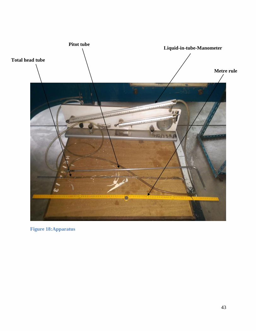
Figure 18:Apparatus
Total head tube
Metre rule
Pitot tube Liquid-in-tube-Manometer

44
6.4 PROCEDURE
The Pitot tube has several holes drilled around the perimeter perpendicular to the direction of
flow and a hole drilled down the center axis aligned parallel to the flow. Static pressure flow is
measured by the holes on the outside, which are connected to one port of a pressure transducer
(liquid-in-tube manometer). The center hole then measures the stagnation pressure, which is
connected to a different port of the pressure transducer.
A pitot tube, total head tube and anemometer measured both the stagnation pressure and static
pressure which were used to calculate the free stream velocity of the flow in the wind tunnel,.
First, the Pitot tube was inserted through holes drilled on the walls of the small test section and
bent at a 90-degree angle to point directly into the flow. This was done for all the holes drilled
vertically on the holes of the small Test Section one and two.
Secondly, the Total head tube was inserted through the holes drilled in Test Section one and two,
and the above procedure repeated for all vertically drilled holes.
Thirdly, the anemometer was inserted through the holes drilled in Test Section one and two, and
the above procedure repeated for all vertically drilled holes.
6.5 REASONS FOR CALIBRATION
Water-in-tube manometers combined with large bore Pitot tubes have low sensitivity to small
static and dynamic pressures and hence pose a difficulty to getting velocities in the wind tunnel
cross-sections. This project therefore needed a measuring system that was more sensitive to
pressure changes hence enabling specific velocity calculations. The measuring system had to
provide a platform for the determination of velocities in a credible manner.
On this note, the total head tube that had a small bore was calibrated to enable pressure
measurement.
In order to calculate velocity from the pressure results from the manometer, the following steps
were taken:-
Velocity calculation from Bernoulli’s principle
√

45
Atmospheric Pressure 24.45inHg=621.03mmHg
Room Temperature 250C
Manometer inclination 0.2
Density of air: A perfect gas is characterized by the perfect gas equation.
From the table of thermodynamic properties of air at room temperature and pressure:
Sample calculation for the data above:
√
T(K) ρ (Kg/m3)
275 1.284
(25+273=298) Ρ
300 1.177
ρair(298) 1.186
Table 3: Thermodynamic table properties.
Source : G.F.C Rogers and Y. Mayhew. Thermodynamic and Transport properties of fluids,5th
Edition 1995.

46
These equations were used to determine the velocity values along the wind tunnel cross-section
in the vertical direction. These values compared to the anemometer and the Pitot tube at
corresponding heights were tabled as shown on table 3.
Height (cm) Pitot Pressure Head (cmH20)
Total Head Pressure Head (cmH20)
Pitot tube velocity (m/s)
Total Head tube velocity (m/s)
Anemometer velocity (m/s)
0 0.4 0.48 3.6 4 4
3 0.5 0.53 4.1 4.2 4.1
6 0.6 0.59 4.5 4.4 4.2
9 0.6 0.56 4.5 4.3 4.3
12 0.6 0.56 4.5 4.3 4.3
15 0.5 0.53 4.1 4.2 4.4
18 0.6 0.56 4.5 4.3 4.4
21 0.6 0.59 4.5 4.4 4.4
24 0.6 0.59 4.5 4.4 4.4
27 0.5 0.56 4.1 4.3 4.3
30 0.5 0.53 4.1 4.2 4.2
33 0.5 0.51 4.1 4.1 4.1
36 0.5 0.51 4.1 4.1 4.1
39 0.5 0.48 4.1 4 4
42 0.5 0.48 4.1 4 3.9
Table 4: Velocity values for different measuring instruments.

47
6.6 VOLUME FLOW RATE COMPUTATIONS
The volume flow rate computations were approached from established methods for square duct
volume discharge measurements namely:-
Method of least squares.
Navier-Stokes equation for square ducts.
6.6.1 Method of least squares.
This involves the use of integration methods where a large area is divided into very small
sections where the properties on that small section are assumed constant.
The large area cross-section of the wind tunnel was divided into small cross-sections of area and
the local velocities measured at this point (i.e. that apply to the small area), an approximate
solution of the volume discharge of a square cross-section was determined by applying the
discharge equation Q=AV.
The Total head water-tube manometer measurements were recorded then tabulated as shown on
table 11-16 in the appendix:-
The velocities were then determined by using the following equation:
√
The velocities were then tabulated as follows in tables 5-10:-

48
Measuring
Points
X1 X2 X3 1 2 3 4 5 6 7 8 9 10 X4 X5 X6
0 3.7 3.9 4 4.2 4.2 4.2 4.1 4.1 4 4.2 4.1 4.1 4.2 4 3.9 3.7
3 3.8 4 4.3 4.4 4.3 4.1 4.2 4.3 4.2 4.2 4.2 4.1 4.3 4.1 3.9 3.8
6 3.9 4.1 4.2 4.5 4.3 4 4.2 4.3 4.4 4.3 4.3 4.2 4.3 4 4 3.9
9 3.8 4 4.1 4.3 4.4 4.1 4.3 4.3 4.3 4.4 4.1 4.2 4.2 3.9 4.1 3.8
12 3.9 3.9 4.2 4.4 4.4 4.2 4.4 4.3 4.3 4.4 4.2 4.2 4.2 4 4.1 3.9
15 4 4.1 4.2 4.3 4.4 4.4 4.4 4.3 4.2 4.4 4.4 4.3 4.3 4.1 4 3.9
18 3.8 3.9 4 4.2 4.3 4.3 4.3 4.4 4.3 4.3 4.2 4.4 4.3 4.2 4.1 4
21 3.8 3.8 4 4.1 4.2 4.3 4.2 4.4 4.4 4.2 4.2 4.4 4.2 4.1 4 3.8
24 4 4.2 4.3 4.4 4.2 4.3 4.2 4.2 4.4 4.2 4.2 4.3 4.2 4 4 3.9
27 4 4.3 4.4 4.5 4.1 4.3 4.2 4.2 4.3 4.1 4.2 4.2 4.3 4.2 4.1 4
30 3.9 4 4.1 4.4 4.3 4.2 4.2 4.1 4.2 4.1 4.2 4.2 4.4 4.3 4.1 3.9
33 3.9 4 4.2 4.4 4.2 4.1 4.1 4.1 4.1 4.1 4.1 4.1 4.3 4.1 3.9 3.9
36 3.9 4 4.1 4.2 4.1 4 4.1 4 4.1 4.1 4 4.1 4.2 4.1 3.8 3.7
39 3.8 3.9 4 4.1 4.1 4 4 4 4 4 4 4 4.1 4 3.9 3.7
42 3.7 3.8 3.9 4 4 4 4 4 4 4 4 4 4 3.9 3.8 3.7
Table 5: Velocities at Test Section One at Speed One.

49
Measuring
Points
1 2 3 4 5 6 7 8 9 10 11 12
0 1 1.3 1.5 1.7 1.8 1.8 1.5 1.2 1.1 1.1 1 0.8
5 1.1 1.6 1.9 2 2.3 2.3 2 1.6 1.3 1.4 1.3 1
10 1.3 1.9 2 2.3 2.5 2.6 2.1 1.9 1.7 1.8 1.6 1.3
15 1.4 2 2.1 2.3 2.6 2.8 2.6 2.3 2.2 2.1 1.9 1.4
20 1.3 1.9 2.3 2.5 2.7 2.8 2.7 2.4 2.4 2.3 2.1 1.5
25 1.4 2 2 2.5 2.8 2.7 2.7 2.6 2.5 2.3 1.7 1.5
30 1.3 1.9 2.2 2.5 2.8 2.7 2.6 2.5 2.6 2.4 1.6 1.4
35 1.5 1.7 2.1 2.3 2.6 2.6 2.6 2.5 2.6 2.3 2 1.3
40 1.5 1.6 1.9 2.2 2.4 2.5 2.5 2.4 2.4 2.1 2 1.3
45 1.3 1.5 1.8 1.7 2.1 2.2 2.3 2.3 2.3 1.9 1.6 1.2
50 1.1 1.5 1.6 1.5 1.8 1.7 2 2.3 1.9 1.7 1.5 1
55 1 1.2 1.3 1.4 1.5 1.2 1.5 2 1.7 1.5 1.5 1
60 0.8 1.1 1.1 1.2 1.1 1.1 1.2 1.8 1.2 1.2 1.3 0.9
65 0.6 0.9 0.6 1 0.8 1 1 1 1 1.1 1 0.8
70 0.5 0.7 0.4 0.8 0.6 0.8 0.9 0.9 0.8 0.7 0.6 0.7
75 0.4 0.5 0.4 0.7 0.5 0.6 0.5 0.7 0.6 0.5 0.5 0.6
Table 6: Velocities at Test Section Two at Speed One.

50
Measurin
g Points
X1 X2 X3 1 2 3 4 5 6 7 8 9 10 X4 X5 X6
0 7.5 7.7 7.9 8 7.9 8.1 8 7.8 7.9 7.9 7.9 7.9 8.1 7.8 7.6 7.4
3 7.6 7.7 7.7 7.9 7.8 8 7.9 7.9 7.9 8.1 7.9 8.1 8.1 7.9 7.7 7.5
6 7.6 7.6 7.9 8 7.7 8 7.9 7.9 8 8.1 8 8.1 8.1 7.8 7.8 7.6
9 7.7 7.7 8 8.1 7.7 7.9 7.9 7.9 8 8.1 8 8.1 8 7.9 7.7 7.6
12 7.8 7.8 7.9 8.1 7.7 7.9 7.9 7.9 8 8.1 7.9 8.1 8 7.8 7.7 7.7
15 7.9 7.9 8 8 7.6 7.9 8.5 8.5 8.5 8.3 7.9 8 8 7.9 7.8 7.8
18 8 8 8 8 7.8 8.1 8.5 8.5 8.5 8.2 8.1 8 8 8 7.9 7.9
21 7.7 7.8 7.8 8.1 7.7 8.1 8.5 8.5 8.5 8.2 8.1 8.2 7.9 7.9 7.7 7.7
24 7.8 7.8 7.9 8.1 7.8 8.2 8.5 8.5 8.5 8.2 8.2 8.2 7.9 7.8 7.6 7.5
27 7.7 7.9 7.9 8 7.8 8.2 8.5 8.5 8.5 8.2 8.2 8.2 7.9 7.7 7.5 7.4
30 7.6 7.7 8.1 8.2 7.9 8.1 8.2 8.1 8.2 8.2 8.3 8.3 8.2 8 7.8 7.6
33 7.6 8 8.2 8.3 8 8 8.2 8.1 8.1 8.2 8.3 8.2 8.1 8 7.9 7.7
36 7.7 8 8.1 8.2 7.9 8 8 8 8 8.1 8.2 8.1 8 7.7 7.6 7.5
39 7.6 7.8 7.8 8.1 8.1 8.1 8.1 8 7.9 8.1 8 8 8 7.6 7.6 7.5
42 7.6 7.7 7.7 8 7.9 7.9 7.8 7.9 7.8 8 7.9 7.9 7.9 7.5 7.5 7.4
Table 7: Velocities at Test Section One at Speed Two.

51
Measuring
Points
1 2 3 4 5 6 7 8 9 10 11 12
0 2.5 2.8 3 3.2 3.3 3.4 3.3 3 2.7 2.6 2.4 2.2
5 2.7 3.3 3.6 3.7 3.7 4.2 3.7 3.6 3.3 3.2 2.6 2.5
10 3 3.5 3.8 4.5 4.6 4.8 4.2 4 3.8 3.5 3.3 2.9
15 3.1 3.7 4.1 4.7 4.9 5.1 4.6 4.5 4 3.8 3.5 2.8
20 3.1 4 4.3 5 5 5.1 5 4.9 4.3 4 3.7 3
25 3.3 4 4.5 5 5.1 5.2 5.1 5 4.5 4.3 3.9 3.2
30 3.4 3.8 4.3 4.9 5 5 5.1 4.9 4.6 4.2 3.8 3.1
35 3 3.8 4.2 4.8 4.8 4.9 4.9 4.7 4.5 4.1 3.5 3.2
40 3.5 3.8 4.1 4.3 4.6 4.7 4.3 4.5 4.5 4.2 3.7 3
45 3 3.4 3.5 3.8 3.9 4.2 3.9 3.8 3.6 3.4 3.2 2.9
50 2.9 3.3 3.1 3.5 3.6 3.6 3.5 3.4 3.3 3.2 2.8 2.7
55 2.7 2.9 2.7 2.8 2.7 2.7 2.9 2.7 2.5 2.4 2.6 2.3
60 1.9 2.2 1.9 2 1.9 2.3 2.1 2.3 2.2 2.1 2 1.8
65 1.8 2.1 1.7 2.1 1.9 1.6 1.9 1.8 2.1 1.7 1.6 1.5
70 1.7 2 1.6 2 1.9 1.6 1.8 1.7 2 1.7 1.5 1.4
75 1.5 1.6 1.6 1.9 1.8 1.6 1.8 1.7 1.9 1.7 1.5 1.4
Table 8: Velocities at Test Section Two at Speed Two.

52
Measuring
Points
X1 X2 X3 1 2 3 4 5 6 7 8 9 10 X4 X5 X6
0 14.5 14.8 14.9 15 15.1 15.1 15.1 15.1 15.1 15 15 15 15 14.8 14.7 14.6
3 14.5 14.6 14.6 14.6 14.9 14.6 15 15 14.6 14.8 14.9 14.9 14.7 14.6 14.6 14.5
6 14.6 14.6 14.8 15 14.9 14.8 15.1 15 14.7 14.9 15 15 15.1 15 14.9 14.7
9 14.7 14.8 14.8 15 15 14.6 15 15 15 15 15 14.9 14.9 14.9 14.8 14.8
12 14.7 14.8 14.8 14.8 15.2 14.7 14.8 15 14.8 15 15.1 14.9 15.1 15 15 14.9
15 14.7 14.8 14.9 14.7 14.6 14.9 15.1 15.1 14.8 15 15.1 14.9 15.1 14.9 14.9 14.8
18 14.8 14.9 15 15 15 15.1 15.1 15.1 14.9 15.2 15.3 15 15.1 15 15 15
21 14.8 15 15 15.1 15.2 15 15 15.1 15.1 15 15.1 14.9 15.1 15 14.9 14.9
24 14.9 15 15.1 15.2 15.1 15.1 15.1 15 15 14.9 15 15 15.3 15.2 15 14.9
27 14.8 14.9 15 15.2 15 15.2 15.2 15 15 14.9 15 15 15.3 15.1 15 15
30 14.8 14.8 14.9 15 15.6 15.4 15.3 15 15 15.2 15.1 15 15.4 15.3 15.2 15.1
33 15 15.2 15.3 15.4 15 15.1 15.3 15.1 15 15 15.3 15.3 15 14.9 14.8 14.7
36 14.7 14.9 15 15.2 15 15.1 15.2 15 14.9 14.9 15.1 15.2 14.9 14.7 14.6 14.5
39 14.6 14.8 14.9 15 14.9 15 15 15 14.8 14.8 14.9 15 14.8 14.6 14.6 14.5
42 14.5 14.7 14.7 14.8 14.9 14.9 14.9 15 14.8 14.9 14.9 14.8 14.8 14.6 14.5 14.5
Table 9: Velocities at Test Section One at Speed Three.

53
Measuring
Points
1 2 3 4 5 6 7 8 9 10 11 12
0 4.3 5.6 6.5 7.5 7.5 7.5 7.5 7.3 7 6 5.3 4.8
5 5.4 6.2 7.4 8.8 9 9.1 8.6 7.9 7.5 6 5.8 5.5
10 5.5 6.4 8.3 9 9.2 9.2 9.3 8.7 7.8 6.5 6.4 6
15 5.6 6.6 8.4 9.2 9.5 9.7 9.5 9.3 8.7 8 7.2 6.7
20 5.8 6.5 8.5 9.5 9.6 9.7 9.5 9.6 8.9 8.4 7.8 7.3
25 5.7 7 8.6 8.7 9 9.5 9.7 9.5 9 8.5 7.9 7.4
30 5.6 7 8.6 8.5 8 9.3 9.4 9.8 9.2 8.8 8.2 7
35 5.6 7 7.5 8.3 8.7 8.6 8.5 9 8.8 8.1 7.6 6.3
40 5.8 6 6 7.8 7.8 7.7 7.6 8.4 8 7.3 6.5 5.5
45 5 6.1 5.7 6.2 7.5 7.4 7.3 7.5 7.2 6.5 5.7 4.8
50 4.6 5 4.5 5.6 6 6 6.1 6.5 6.1 5.6 4.8 4.1
55 4.3 4 3 4.2 5.7 4.9 4.8 4.7 4.8 4.8 3.8 3.6
60 3.4 3.3 2.9 3.5 4.8 3 3.9 4.4 3.6 3.6 2.9 2.7
65 2.2 2.5 2.5 2.5 3.9 2.6 2.8 3 2.9 2.8 2.4 2.1
70 2.1 2.3 2.3 2.4 3 2.4 2.6 2.9 2.5 2.5 2.3 2
75 2 2.2 2.2 2.3 2.5 2.3 2.4 2.5 2.3 2.3 2.1 2
Table 10: Velocities at Test Section Two at Speed Three.

54
The above velocities were used to get the volume flow rate that passed through each of the small
sections as shown in the sample calculations:-
Sample calculation for Test Section 1 at speed 1.
Using the equation:
Sample calculation for Test Section 2 at speed 1.
Using the equation:
0.003125
Percentage Flow Rate Loss at speed 1
Sample calculation for Test Section 1 at speed 2.
Using the equation:
/s

55
Sample calculation for Test Section 2 at speed 2.
Using the equation:
0.003125 /s
Percentage Flow Rate Loss at speed 2
Sample calculation for Test Section 1 at speed 3.
Using the equation:
0.001125 /s
Sample calculation for Test Section 2 at speed 3.
Using the equation:
0.003125
/s
Percentage Flow Rate Loss at speed 3.

56
6.6.2 Navier Stokes equation for square ducts
, where,
Calculation for Test Section 1 at speed 1.
At speed 1:
Pa/m
Then:
-205.18891
Using the equation:
Calculation for Test Section 2 at speed 1
At speed 1:
Pa/m
Then:
Using the equation:
=1.029

57
Percentage Flow Rate Loss at speed 1.
Calculation for Test Section 1 at speed 2.
At speed 2:
Pa/m
Then:
Using the equation:
Calculation for Test Section 2 at speed 2.
At speed 2:
Pa/m
Then:
Using the equation:
=2.054719 /s
Percentage Flow Rate Loss at speed 2.

58
Calculation for Test Section 1 at speed 3.
At speed 3:
Pa/m
Then:
=743.61753
Using the equation:
Calculation for Test Section 2 at speed 3
At speed 3:
Pa/m
Then:
Using the equation:
=
Percentage Flow Rate Loss at speed 3.

59
6.7 DISCUSSION FOR THE EXPERIMENTS
For computation of volume flow rates, two methods were utilized;
Method of least squares- The effect of the boundary layer at the walls of each section was
accounted for by measuring the velocities at the wall.
Navier-Stokes equation for square ducts- At the walls of each section, the no-slip
condition was assumed hence a velocity of zero was adopted at this point for all sections.
The discharge varied from the small test section to the exit section. The method of least squares
gave an average of 11% loss in discharge, while the Navier-Stokes method gave an average of
10.7% loss in discharge.
The Navier-Stokes method offered a theoretical approach to the analysis. Since the method of
least squares accounted for effect of the boundary layer, it was assumed to accurately show the
velocity and flow rate in the wind tunnel.
The above difference in volume flow rate was attributed to:-
Faulty Setting up of Equipment: Inspite of our best efforts to ensure credibility of the results,
accumulated errors might have resulted from the continuous setting up of the equipment causing
discrepancies in the instrument readings that could cause difference in velocity readings hence
difference in flow rate.
Leakages: Inspite of our best efforts to minimize loss, There were leakages on the wind tunnel
seams that could cause reduction in flow rate.

60
6.7.1 OBSERVATIONS
6.7.1.1 TEST SECTION ONE
Test Speed 1
The observed range of velocities was from 3.7 m/s to 4.5 m/s. They were drawn as shown in
graph 1, varying from a blue color, representing the lowest speeds to a dark red color,
representing the highest speeds. The 3D velocity visualization did not show a smooth velocity
profile with peaks at regions that were presumed to be low velocity regions and dips at regions
presumed to be high velocity regions.
The corresponding Isovels for the above 3D graph showed regions of the low velocities at the
boundaries ranging from 3.7 to 3.9 m/s as shown in graph 2. The central regions showed a
variation of wind speeds between 4.2 to 4.5 m/s. The Isovel for test speed one showed areas of
constant velocity but these areas had regions with high and low velocities within them. The
lowest velocities observed were at the corners.
Graph 3 showed the 3D flow rate visualization at this test speed. This graph wass similar to the
velocity visualization in graph 1 except for the range of flow rates which is from to
.
Test Speed 2
The measured speeds ranged from 7.4m/s to 8.6 m/s and were depicted by dark red and blue
colours respectively in graph 4. The 3D velocity visualization showed a velocity profile similar
to the theoretical profile expected. There was a gradual increase in velocity from the boundaries
with the peak velocities achieved at the central regions.
From graph 5, the Isovels enclosed regions of low velocities at the boundaries, represented by
blue colour. The central region contains areas with high velocities with minimal interference
between the flow fields. There was discontinuity observed in the velocity regions near the
boundaries. The lowest velocities observed were at the corners.

61
The 3D visualization of flow rates was as shown in graph 6 and corresponded to graph 3. The
flow rates ranged from to .
Test Speed 3
The experimental speeds ranged from 14.5 m/s to 15.6 m/s as shown by dark red and blue
colours respectively on graph 7. The velocity profile had peaks at regions presumed to be low
velocity regions, and dips in regions of high velocity. The dominant velocity region had
velocities ranging from 15 to 15.1 m/s.
Graph 8 showed regions enclosed by Isovels. The central regions had velocities of 14.8 to 15.6
m/s, while at the regions near the boundaries the velocities ranged from 14.5 to 14.7 m/s. The
lowest velocities observed were at the corners. The areas that showed a gradual rise in velocities
were at the central region.
Graph 9 showed a 3D visualization of flow rates at this test section. This visualization
corresponded to the velocity profile observed in graph 7. The flow rates range from
to .
6.7.1.2 TEST SECTION TWO
Test Speed 1
The velocity profile in graph 10 was smooth with velocities ranging from 0.5 to 2.8 m/s. There
was a gradual rise velocity from the boundaries with peak speeds achieved in the central region.
Graph 11 showed regions with equal velocities (Isovels) smoothly enclosed in the same area.
The lowest velocities occurred in the corners of the cross section. The speeds were distributed
evenly in approximately equal regions having 1.5 m/s to 2.6 m/s. The upper region had quite low
velocities ranging from 0.5 to 1 m/s.
The flow rate visualization in graph 12 corresponded to the velocity profile in graph 10, with the
flow rate ranging from to .

62
Test Speed 2
From graph 13, the speeds ranged from 1m/s to 5 m/s. There was a gradual rise in velocity that
generated a smooth profile. The lowest speeds were attained at the boundaries and peaks
achieved at the central region.
Graph 14 showed the lowest velocities occurred at the corners The Isovels enclosed regions with
equal velocities. The central region had velocities ranging from 3.5 to 5.5 m/s. The top part of
the graph depicted a region of low velocities in the upper region of the cross section, which was
approximately a quarter of the cross section.
The 3D visualization of the flow rates as seen in graph 15 depicted great similarities to the
velocity profile in graph 13. The flow rate ranged from to .
Test Speed 3
From graph 16, there was a gradual rise of velocity from 2 to 10 m/s. The profile generated was
smooth with peak velocities being at a mean of 10 m/s.
Graph 17 shown regions of equal velocities enclosed by Isovels. The highest velocities recorded
were in the central region, which showed bias towards the lower part of the cross section. The
lowest velocities observed were at the upper part of the cross section, covering a quarter of the
cross section.
The flow rates visualization in graph 18 corresponded to the profile in graph 16. The flow rates
ranged from to .

63
6.7.2 GENERAL OBSERVATIONS
Test Section 1
There was no consistency in the velocity profiles generated by the experimental results. The
Isovels showed mixed velocity regions where regions of low velocity had regions within them
that had high velocity and vice versa. The 3D graphs at test speed 1 and 3 showed similar
characteristics while the one at speed 2 broke the trend.
Test Section 2
The velocity profiles generated from the experimental results were smooth in all the test speeds.
The Isovels enclosed regions with the same velocities, with minimal reductions observed. The
upper quarter of the cross section consistently showed a region of low velocity in all the test
velocities. The velocities progressively rose from regions next to the boundaries to the central
regions in the three test velocities. The 3D graphs at all the test speeds had similar
characteristics.
6.7.3 INTERPRETATION
Test Section 1
The regions enclosed by Isovels had areas within them that were at velocities higher or lower
than the speeds in the region. This was attributed to the following factors:
i. Errors in velocity measurement- In ducts, smooth velocity profiles are usually
expected, but the velocity profiles obtained from experimental data portray
unexpected peaks and dips. This was thought to be a result of the following:
Vibrations from the motor caused significant changes in manometric readings due to
the shaking.
The inability of the manometer to respond rapidly to the changing high velocity
pressures across the cross section.
ii. Parallax errors in manometer readings.

64
iii. The current wind tunnel designs call for hexagonal honeycombs and screens as flow
straighteners. Screens are used to reduce turbulence especially when used in a
cascading series. Each screen increases the turbulence reduction through a
combination of decrease in the scale of the turbulence and inducing small-scale
turbulence in the flow. It is recommended that the screens should have a less dense
mesh at the inlet of the screens and a more dense mesh at the outlet. Investigation of
the type of flow straighteners used in the department's wind tunnel was impossible
due to lack of permission to dismantle the tunnel from the concerned authorities.
iv. The wind tunnel used in this project is a circa 1970-wind tunnel, whereas these
guidelines were established after 1984, hence the flow straighteners used in it might
not be sufficient to reduce turbulence.
v. Particle entrainment due to poor maintenance
vi. The wind tunnel used in this project is not frequently serviced, hence increased
turbulence intensity. The fans, the settling chamber, stands, and motor have not gone
through any maintenance procedures.
vii. Flow separation in contraction and diffuser sections due to insufficient
accommodation of changing cross-sectional area.
The low velocities observed at the corners of the cross section was attributed to the reduction of
velocities due to boundary layer effect.

65
Test Section 2
In this section, there was consistency in the velocity flow fields, which were concentric to the
region of highest velocity. The upper quarter of the cross section was found to have low
velocities profiles.
This was attributed to:
The flow settling in the chamber causing flow to settle in the lower regions
The viscous flow due to drag at the upper section of the profile.
The velocity profiles from the 3D visualization graphs were smooth and consistent. The location
of the Isovels with highest wind speed was towards the bottom of the wind tunnel. The velocities
recorded at this Test Section were consistently lower than those in test section one.This was
attributed to:
i. The effect of diffuser section on the wind tunnel speed.
ii. The pressure differential after wind speed reduction in the diffuser.
The above interpretation shown that the test section 1 might not give accurate results when
testing a model in it. This was due to the varying wind speeds found within the cross section.
However, at the regions of very low speeds, the planes affected by boundary layer were avoided.
An approximate wind speed can be chosen in subsequent experiments and the variation factored
in by use of the Isovels given above.
At the large section, model placement could be optimized to take advantage of the lower three
quarter of the cross section. This region has low variation in velocity as shown in the Isovels.
Future models should be designed to take advantage of the Isovels that we showed above for
accurate analysis of data.

66
CHAPTER 7: RECOMMENDATIONS AND CONCLUSION
7.1 RECOMMENDATION
In this thesis, the Isovels and flow rates in test section one and test section two were established
after minimizing losses by sealing possible leakage sections. The volume flow rate between test
section one and test section two were compared to establish the difference. This served to
explore the drawbacks of the wind tunnel at the department of Mechanical and Manufacturing
Engineering, which could be used to correct results from it.
Further improvements can be done by:
1) Redesign of the wind tunnel. The wind tunnel rectangular cross section could be replaced
by a circular or hexagonal cross section that could minimize turbulence and errors and
flow straightening section to reduce turbulence further.
2) Use of small bore Pitot tubes that effectively measure small pressure differentials.
3) Upgrade of the wind tunnel. The wind tunnel can be upgraded by using newer designs
standards especially in the flow straightening section to reduce turbulence further.
4) Students could undertake a study to establish the velocity deficit caused by the fans.
5) To enable more accurate results, total friction and viscous drag coefficients for this tunnel
could be established.
6) The use of multi-point hot anemometers, which facilitate instant establishment of flow
across a section.
7) Measuring supports could be introduced to assist in getting accurate results also make
work easier.

67
7.2 CHALLENGES
The following are challenges we encountered during the project:
Time limitation: The time allocated for the project was limited, since it was done in
combination with other courses through the whole academic year. The scope of the
project was wide and required deep research.
Financial Constraint: The materials used had to be economically viable and substitutes
made for resources that were beyond the range of our set budget. The design had to
involve experts in carpentry which had to be outsourced from another department hence
higher overheads.
Technological Constraint: For measurement of pressure across small distances the Pitot
tube was not sensitive enough, therefore there was need for re-evaluation of the same
pressures using a total head tube.
7.3 CONCLUSION
The objective of this thesis was to calibrate the wind tunnel by measuring the velocities hence
establishing the velocity profiles and flow rates and calibration of associated measuring probes.
It was found that the velocity profiles for test section one were not consistent which was
attributed to turbulence, while that of test section two approached the expected profiles.
It was ascertained that the difference in volumetric flow rates in test section one and two differed
by an approximately 11%. A simple equation to enable the comparison of the flow rates was
used as shown below.
Where - flow rate at test section 1
- Flow rate at test section 2
k- Volume flow constant =0.89
It was found that the boundary layer at the corners of the test section affected the flow and
velocity profiles.

68
REFERENCES
1. Josue Njock Libii (2011).Wind Tunnels in Engineering Education, Wind Tunnels and
Experimental Fluid Research. ISBN 978-953-307-623-2.
2. R.D Mehta and P. Bradshaw, Design Rules for small low speed wind tunnels,
Aeronautical Journal. Royal Aeronautical Society,1979.
3. Bell, J.H and R.D Mehta, Construction Design for Small Low-Speed Wind Tunnels
(NASA Contractor Report) NASA CR-177488 Washington DC: National Acoustics and
Space Administration, (1988).
4. Barlow, Jewel B, William H, Rae and Alan Pope, Low-speed Wind Tunnel Testing, 3rd
Edition, New York, Wiley Inter Science, (1999).
5. Wind Program, History of Wind Energy. US Department of Energy, (September 2011).
6. Prof S.B Kedare, Wind Conversion Systems, Bombay, Indian Institute of Technology,
P.S, (2003).
7. Aerodynamics for students, University of Sydney School of Aerospace, Mechanical and
MechatronicsEngineering,09April2009.http://sites.google.com/site/aerodynamics4student
s
8. John A. Roberson, Clayton T. Crowe, Engineering Fluid Mechanics, Washington State
University, Pullman.(1974)
9. M. Bahrami, Fluid Mechanics (S 09)
10. Colin Mitchell, Measuring the Air Created in Wind Tunnel, Pomona College, April 26,
2013.
11. N. Thaweewat, Wind Tunnel (REPORT), International Maritime Collage, Kasetsart
University, Thailand.
12. http://www.formula1-dictionary.net/wind_tunnel.html

69
APPENDICES
Measuring
Points
X1 X2 X3 1 2 3 4 5 6 7 8 9 10 X4 X5 X6
0 0.11 0.12 0.12 0.13 0.13 0.13 0.12 0.12 0.12 0.13 0.12 0.12 0.13 0.12 0.12 0.11
3 0.11 0.12 0.13 0.13 0.13 0.12 0.13 0.13 0.13 0.13 0.13 0.12 0.13 0.12 0.12 0.11
6 0.12 0.12 0.13 0.14 0.13 0.12 0.13 0.13 0.13 0.13 0.13 0.13 0.13 0.12 0.12 0.12
9 0.11 0.12 0.12 0.13 0.13 0.12 0.13 0.13 0.13 0.13 0.12 0.13 0.13 0.12 0.12 0.11
12 0.12 0.12 0.13 0.13 0.13 0.13 0.13 0.13 0.13 0.13 0.13 0.13 0.13 0.12 0.12 0.12
15 0.12 0.12 0.13 0.13 0.13 0.13 0.13 0.13 0.13 0.13 0.13 0.13 0.13 0.12 0.12 0.12
18 0.11 0.12 0.12 0.13 0.13 0.13 0.13 0.13 0.13 0.13 0.13 0.13 0.13 0.13 0.12 0.12
21 0.11 0.11 0.12 0.12 0.13 0.13 0.13 0.13 0.13 0.13 0.13 0.13 0.13 0.12 0.12 0.11
24 0.12 0.13 0.13 0.13 0.13 0.13 0.13 0.13 0.13 0.13 0.13 0.13 0.13 0.12 0.12 0.12
27 0.12 0.13 0.13 0.14 0.12 0.13 0.13 0.13 0.13 0.12 0.13 0.13 0.13 0.13 0.12 0.12
30 0.12 0.12 0.12 0.13 0.13 0.13 0.13 0.12 0.13 0.12 0.13 0.13 0.13 0.13 0.12 0.12
33 0.12 0.12 0.13 0.13 0.13 0.12 0.12 0.12 0.12 0.12 0.12 0.12 0.13 0.12 0.12 0.12
36 0.12 0.12 0.12 0.13 0.12 0.12 0.12 0.12 0.12 0.12 0.12 0.12 0.13 0.12 0.11 0.11
39 0.11 0.12 0.12 0.12 0.12 0.12 0.12 0.12 0.12 0.12 0.12 0.12 0.12 0.12 0.12 0.11
42 0.11 0.11 0.12 0.12 0.12 0.12 0.12 0.12 0.12 0.12 0.12 0.12 0.12 0.12 0.11 0.11
Table 11: Pressure difference (m) at Test Section one at Speed one.

70
Measuring
Points
1 2 3 4 5 6 7 8 9 10 11 12
0 0.03 0.04 0.05 0.05 0.05 0.05 0.05 0.04 0.03 0.03 0.03 0.02
5 0.03 0.05 0.06 0.06 0.07 0.07 0.06 0.05 0.04 0.04 0.04 0.03
10 0.04 0.06 0.06 0.07 0.08 0.08 0.06 0.06 0.05 0.05 0.05 0.04
15 0.04 0.06 0.06 0.07 0.08 0.08 0.08 0.07 0.07 0.06 0.06 0.04
20 0.04 0.06 0.07 0.08 0.08 0.08 0.08 0.07 0.07 0.07 0.06 0.05
25 0.04 0.06 0.06 0.08 0.08 0.08 0.08 0.08 0.08 0.07 0.05 0.05
30 0.04 0.06 0.07 0.08 0.08 0.08 0.08 0.08 0.08 0.07 0.05 0.04
35 0.05 0.05 0.06 0.07 0.08 0.08 0.08 0.08 0.08 0.07 0.06 0.04
40 0.05 0.05 0.06 0.07 0.07 0.08 0.08 0.07 0.07 0.06 0.06 0.04
45 0.04 0.05 0.05 0.05 0.06 0.07 0.07 0.07 0.07 0.06 0.05 0.04
50 0.03 0.05 0.05 0.05 0.05 0.05 0.06 0.07 0.06 0.05 0.05 0.03
55 0.03 0.04 0.04 0.04 0.05 0.04 0.05 0.06 0.05 0.05 0.05 0.03
60 0.02 0.03 0.03 0.04 0.03 0.03 0.04 0.05 0.04 0.04 0.04 0.03
65 0.02 0.03 0.02 0.03 0.02 0.03 0.03 0.03 0.03 0.03 0.03 0.02
70 0.02 0.02 0.01 0.02 0.02 0.02 0.03 0.03 0.02 0.02 0.02 0.02
75 0.01 0.02 0.01 0.02 0.02 0.02 0.02 0.02 0.02 0.02 0.02 0.02
Table 12: Pressure difference (m) at Test Section two at Speed one.

71
Measuring
Points
X1 X2 X3 1 2 3 4 5 6 7 8 9 10 X4 X5 X6
0 0.23 0.23 0.24 0.24 0.24 0.24 0.24 0.24 0.24 0.24 0.24 0.24 0.24 0.24 0.23 0.22
3 0.23 0.23 0.23 0.24 0.24 0.24 0.24 0.24 0.24 0.24 0.24 0.24 0.24 0.24 0.23 0.23
6 0.23 0.23 0.24 0.24 0.24 0.24 0.24 0.24 0.24 0.24 0.24 0.24 0.24 0.24 0.24 0.23
9 0.23 0.23 0.24 0.25 0.25 0.25 0.26 0.26 0.26 0.25 0.25 0.25 0.25 0.24 0.23 0.23
12 0.24 0.24 0.24 0.25 0.25 0.25 0.26 0.26 0.26 0.25 0.25 0.25 0.25 0.24 0.23 0.23
15 0.24 0.24 0.24 0.25 0.25 0.25 0.26 0.26 0.26 0.25 0.25 0.25 0.25 0.24 0.24 0.24
18 0.24 0.24 0.25 0.25 0.25 0.25 0.25 0.26 0.26 0.25 0.25 0.25 0.25 0.24 0.24 0.24
21 0.23 0.24 0.24 0.25 0.25 0.25 0.26 0.26 0.25 0.25 0.25 0.25 0.25 0.24 0.23 0.23
24 0.24 0.24 0.24 0.25 0.25 0.25 0.26 0.26 0.26 0.25 0.25 0.25 0.25 0.24 0.23 0.23
27 0.23 0.24 0.24 0.25 0.25 0.25 0.26 0.26 0.26 0.25 0.25 0.25 0.25 0.24 0.23 0.22
30 0.23 0.23 0.24 0.25 0.25 0.25 0.25 0.26 0.25 0.25 0.25 0.25 0.25 0.24 0.24 0.23
33 0.23 0.24 0.25 0.25 0.25 0.25 0.25 0.25 0.24 0.25 0.25 0.25 0.24 0.24 0.24 0.23
36 0.23 0.24 0.24 0.25 0.25 0.25 0.25 0.25 0.25 0.24 0.25 0.24 0.24 0.24 0.23 0.23
39 0.23 0.24 0.24 0.24 0.24 0.24 0.24 0.24 0.24 0.24 0.24 0.24 0.24 0.23 0.23 0.23
42 0.23 0.23 0.23 0.24 0.24 0.24 0.24 0.24 0.24 0.24 0.24 0.24 0.24 0.23 0.23 0.22
Table 13: Pressure difference (m) at Test Section one at Speed two.

72
Measuring Points
1 2 3 4 5 6 7 8 9 10 11 12
0 0.08 0.08 0.09 0.10 0.10 0.10 0.10 0.09 0.08 0.08 0.07 0.07
5 0.08 0.10 0.11 0.11 0.11 0.13 0.11 0.11 0.10 0.10 0.08 0.08
10 0.09 0.11 0.11 0.14 0.14 0.15 0.13 0.12 0.11 0.11 0.10 0.09
15 0.09 0.11 0.12 0.14 0.15 0.15 0.14 0.14 0.12 0.11 0.11 0.08
20 0.09 0.12 0.13 0.15 0.15 0.15 0.15 0.15 0.13 0.12 0.11 0.09
25 0.10 0.12 0.14 0.15 0.15 0.16 0.15 0.15 0.14 0.13 0.12 0.10
30 0.10 0.11 0.13 0.15 0.15 0.15 0.15 0.15 0.14 0.13 0.11 0.09
35 0.09 0.11 0.13 0.15 0.15 0.15 0.15 0.14 0.14 0.12 0.11 0.10
40 0.11 0.11 0.12 0.13 0.14 0.14 0.13 0.14 0.14 0.13 0.11 0.09
45 0.09 0.10 0.11 0.11 0.12 0.13 0.12 0.11 0.11 0.10 0.10 0.09
50 0.09 0.10 0.09 0.11 0.11 0.11 0.11 0.10 0.10 0.10 0.08 0.08
55 0.08 0.09 0.08 0.08 0.08 0.08 0.09 0.08 0.08 0.07 0.08 0.07
60 0.06 0.07 0.06 0.06 0.06 0.07 0.06 0.07 0.07 0.06 0.06 0.05
65 0.05 0.06 0.05 0.06 0.06 0.05 0.06 0.05 0.06 0.05 0.05 0.05
70 0.05 0.06 0.05 0.06 0.06 0.05 0.05 0.05 0.06 0.05 0.05 0.04
75 0.05 0.05 0.05 0.06 0.05 0.05 0.05 0.05 0.06 0.05 0.05 0.04
Table 14: Pressure difference (m) at Test Section two at Speed two.

73
Measurin
g Points
X1 X2 X3 1 2 3 4 5 6 7 8 9 10 X4 X5 X6
0 0.44 0.45 0.45 0.45 0.46 0.46 0.46 0.46 0.46 0.45 0.45 0.45 0.45 0.45 0.44 0.44
3 0.44 0.44 0.44 0.44 0.45 0.44 0.45 0.45 0.44 0.45 0.45 0.45 0.44 0.44 0.44 0.44
6 0.44 0.44 0.45 0.45 0.45 0.45 0.46 0.45 0.44 0.45 0.45 0.45 0.46 0.45 0.45 0.44
9 0.44 0.45 0.45 0.45 0.45 0.44 0.45 0.45 0.45 0.45 0.45 0.45 0.45 0.45 0.45 0.45
12 0.44 0.45 0.45 0.45 0.46 0.44 0.45 0.45 0.45 0.45 0.46 0.45 0.46 0.45 0.45 0.45
15 0.44 0.45 0.45 0.44 0.44 0.45 0.46 0.46 0.45 0.45 0.46 0.45 0.46 0.45 0.45 0.45
18 0.45 0.45 0.45 0.45 0.45 0.46 0.46 0.46 0.45 0.46 0.46 0.45 0.46 0.45 0.45 0.45
21 0.45 0.45 0.45 0.46 0.46 0.45 0.45 0.46 0.46 0.45 0.46 0.45 0.46 0.45 0.45 0.45
24 0.45 0.45 0.46 0.46 0.46 0.46 0.46 0.45 0.45 0.45 0.45 0.45 0.46 0.46 0.45 0.45
27 0.45 0.45 0.45 0.46 0.45 0.46 0.46 0.45 0.45 0.45 0.45 0.45 0.46 0.46 0.45 0.45
30 0.45 0.45 0.45 0.45 0.47 0.47 0.46 0.45 0.45 0.46 0.46 0.45 0.47 0.46 0.46 0.46
33 0.45 0.46 0.46 0.47 0.45 0.46 0.46 0.46 0.45 0.45 0.46 0.46 0.45 0.45 0.45 0.44
36 0.44 0.45 0.45 0.46 0.45 0.46 0.46 0.45 0.45 0.45 0.46 0.46 0.45 0.44 0.44 0.44
39 0.44 0.45 0.45 0.45 0.45 0.45 0.45 0.45 0.45 0.45 0.45 0.45 0.45 0.44 0.44 0.44
42 0.44 0.44 0.44 0.45 0.45 0.45 0.45 0.45 0.45 0.45 0.45 0.45 0.45 0.44 0.44 0.44
Table 15: Pressure difference (m) at Test Section one at Speed three.

74
Measuring
Points
1 2 3 4 5 6 7 8 9 10 11 12
0 0.13 0.17 0.20 0.23 0.23 0.23 0.23 0.22 0.21 0.18 0.16 0.15
5 0.16 0.19 0.22 0.27 0.27 0.28 0.26 0.24 0.23 0.18 0.18 0.17
10 0.17 0.19 0.25 0.27 0.28 0.28 0.28 0.26 0.24 0.20 0.19 0.18
15 0.17 0.20 0.25 0.28 0.29 0.29 0.29 0.28 0.26 0.24 0.22 0.20
20 0.18 0.20 0.26 0.29 0.29 0.29 0.29 0.29 0.27 0.25 0.24 0.22
25 0.17 0.21 0.26 0.26 0.27 0.29 0.29 0.29 0.27 0.26 0.24 0.22
30 0.17 0.21 0.26 0.26 0.24 0.28 0.28 0.30 0.28 0.27 0.25 0.21
35 0.17 0.21 0.23 0.25 0.26 0.26 0.26 0.27 0.27 0.24 0.23 0.19
40 0.18 0.18 0.18 0.24 0.24 0.23 0.23 0.25 0.24 0.22 0.20 0.17
45 0.15 0.18 0.17 0.19 0.23 0.22 0.22 0.23 0.22 0.20 0.17 0.15
50 0.14 0.15 0.14 0.17 0.18 0.18 0.18 0.20 0.18 0.17 0.15 0.12
55 0.13 0.12 0.09 0.13 0.17 0.15 0.15 0.14 0.15 0.15 0.11 0.11
60 0.10 0.10 0.09 0.11 0.15 0.09 0.12 0.13 0.11 0.11 0.09 0.08
65 0.07 0.08 0.08 0.08 0.12 0.08 0.08 0.09 0.09 0.08 0.07 0.06
70 0.06 0.07 0.07 0.07 0.09 0.07 0.08 0.09 0.08 0.08 0.07 0.06
75 0.06 0.07 0.07 0.07 0.08 0.07 0.07 0.08 0.07 0.07 0.06 0.06
Table 16: Pressure difference (m) at Test Section two at Speed three.

75
Table 17: Volume Flow Rate (m3/s) at Test Section one at Speed one.
Measuring
Points X1 X2 X3 1 2 3 4 5 6 7 8 9 10 X4 X5 X6
0 0.004163 0.004388 0.0045 0.004725 0.004725 0.004725 0.004613 0.004613 0.0045 0.004725 0.004613 0.004613 0.004725 0.0045 0.004388 0.004163
3 0.004275 0.0045 0.004838 0.00495 0.004838 0.004613 0.004725 0.004838 0.004725 0.004725 0.004725 0.004613 0.004838 0.004613 0.004388 0.004275
6 0.004388 0.004613 0.004725 0.005063 0.004838 0.0045 0.004725 0.004838 0.00495 0.004838 0.004838 0.004725 0.004838 0.0045 0.0045 0.004388
9 0.004275 0.0045 0.004613 0.004838 0.00495 0.004613 0.004838 0.004838 0.004838 0.00495 0.004613 0.004725 0.004725 0.004388 0.004613 0.004275
12 0.004388 0.004388 0.004725 0.00495 0.00495 0.004725 0.00495 0.004838 0.004838 0.00495 0.004725 0.004725 0.004725 0.0045 0.004613 0.004388
15 0.0045 0.004613 0.004725 0.004838 0.00495 0.00495 0.00495 0.004838 0.004725 0.00495 0.00495 0.004838 0.004838 0.004613 0.0045 0.004388
18 0.004275 0.004388 0.0045 0.004725 0.004838 0.004838 0.004838 0.00495 0.004838 0.004838 0.004725 0.00495 0.004838 0.004725 0.004613 0.0045
21 0.004275 0.004275 0.0045 0.004613 0.004725 0.004838 0.004725 0.00495 0.00495 0.004725 0.004725 0.00495 0.004725 0.004613 0.0045 0.004275
24 0.0045 0.004725 0.004838 0.00495 0.004725 0.004838 0.004725 0.004725 0.00495 0.004725 0.004725 0.004838 0.004725 0.0045 0.0045 0.004388
27 0.0045 0.004838 0.00495 0.005063 0.004613 0.004838 0.004725 0.004725 0.004838 0.004613 0.004725 0.004725 0.004838 0.004725 0.004613 0.0045
30 0.004388 0.0045 0.004613 0.00495 0.004838 0.004725 0.004725 0.004613 0.004725 0.004613 0.004725 0.004725 0.00495 0.004838 0.004613 0.004388
33 0.004388 0.0045 0.004725 0.00495 0.004725 0.004613 0.004613 0.004613 0.004613 0.004613 0.004613 0.004613 0.004838 0.004613 0.004388 0.004388
36 0.004388 0.0045 0.004613 0.004725 0.004613 0.0045 0.004613 0.0045 0.004613 0.004613 0.0045 0.004613 0.004725 0.004613 0.004275 0.004163
39 0.004275 0.004388 0.0045 0.004613 0.004613 0.0045 0.0045 0.0045 0.0045 0.0045 0.0045 0.0045 0.004613 0.0045 0.004388 0.004163
42 0.004163 0.004275 0.004388 0.0045 0.0045 0.0045 0.0045 0.0045 0.0045 0.0045 0.0045 0.0045 0.0045 0.004388 0.004275 0.004163
0.065138 0.067388 0.06975 0.07245 0.071438 0.070313 0.070763 0.070875 0.0711 0.070875 0.0702 0.07065 0.071438 0.068625 0.067163 0.0648 1.112963
Σ
Σ

76
Table 18: Volume Flow Rate (m3/s) at Test Section two at Speed one.

77
Table 19: Volume Flow Rate (m3/s) at Test Section one at Speed two.

78
Table 20: Volume Flow Rate (m3/s) at Test Section two at Speed two.

79
Table 21: Volume Flow Rate (m3/s) at Test Section one at Speed three.

80
Table 22: Volume Flow Rate (m3/s) at Test Section two at Speed three.

81
Figure 19:3-D Velocity Visualisation at Test Section 1 at Test Speed 1.
Graph 1

82
Figure 20:3-D Velocity Visualisation at Test Section 1 at Test Speed 1.
Graph 2

83
Figure 21:3-D Velocity Visualisation at Test Section 1 at Test Speed 1.
Graph 3

84
Figure 22:3-D Velocity Visualisation at Test Section 1 at Test Speed 2.
Graph 4

85
Figure 23:3-D Velocity Visualisation at Test Section 1 at Test Speed 2.
Graph 5

86
Figure 24:3-D Velocity Visualisation at Test Section 1 at Test Speed 2.
Graph 6

87
Figure 19:3-D Velocity Visualisation at Test Section 1 at Test Speed 2.
Graph 7

88
Figure 26:3-D Velocity Visualisation at Test Section 1 at Test Speed 2.
Graph 8

89
Figure 27:3-D Flow Visualisation at Test Section 1 at Test Speed 3.
Graph 9

90
Figure 28:3-D Flow Visualisation at Test Section 2 at Test Speed 1.
Graph 10

91
Figure 29:3-D Velocity Visualisation at Test Section 2 at Test Speed 1.
Graph 11

92
Figure 30 :3-D Flow Visualisation at Test Section 1 at Test Speed 2.
Graph 12

93
Figure 31:3-D Velocity Visualisation at Test Section 2 at Test Speed 2.
Graph 13

94
Figure 32 :3-D Velocity Visualisation at Test Section 2 at Test Speed 2.
Graph 14

95
Figure 33:3-D Flow Visualisation at Test Section 2 at Test Speed 2.
Graph 15

96
Figure 34 :3-D Flow Visualisation at Test Section 2 at Test Speed 3.
Graph 16

97
Figure 35:3-D Flow Visualisation at Test Section 2 at Test Speed 3.
Graph 17

98
Figure 20:3-D Velocity Visualisation at Test Section 2 at Test Speed 3.
Graph 18