the university of melbourne - fbe.unimelb.edu.au€¦ · stokey, lucas and prescott for markov...

ISSN 0819-2642 ISBN 0 7340 2555 6

THE UNIVERSITY OF MELBOURNE

DEPARTMENT OF ECONOMICS

RESEARCH PAPER NUMBER 899

FEBRUARY 2004

PARAMETRIC CONTINUITY OF STATIONARY DISTRIBUTIONS

by

Cuong Le Van &

John Stachurski

Department of Economics The University of Melbourne Melbourne Victoria 3010 Australia.

PARAMETRIC CONTINUITY OF STATIONARYDISTRIBUTIONS

CUONG LE VAN AND JOHN STACHURSKI

Abstract. The paper gives conditions under which stationary

distributions of Markov models depend continuously on the param-

eters. It extends a well-known parametric continuity theorem for

compact state space to the unbounded setting of standard econo-

metrics and time series analysis. Applications to several theoretical

and estimation problems are outlined.

1. Introduction

In macroeconomic dynamics, time series econometrics and other related

fields, one frequently considers economies where the sequence of state

variables (Xt)∞t=0 is stationary. Here Xt is a vector of endogenous and

exogenous variables, jointly following a Markov process generated by

some underlying model. By stationary is meant the existence of a

“stationary distribution” µ, such that if Xt has law µ, then so does

Xt+j for all j ∈ N. If such a µ exists, is unique and has some stability

properties, then it naturally becomes the focus of equilibrium analysis.

For example, in these settings a law of large numbers result often holds,

in which case sample moments from the series (Xt)∞t=0 can be identified

with integrals of the relevant functions with respect to the stationary

distribution µ.

Typically, the underlying laws which drive the process (Xt)∞t=0 depend

on a vector of parameters, which may for example be policy instru-

ments, or regression coefficients to be estimated from the data. In

this case the parameters themselves determine the stationary distribu-

tion. The study of how this distribution varies with the parameters is a1

2 CUONG LE VAN AND JOHN STACHURSKI

stochastic analogue of standard comparative dynamics. Our paper in-

vestigates conditions under which the functional relationship between

parameters and stationary distribution is continuous.

The main results extend directly a well-known and useful argument in

Stokey, Lucas and Prescott for Markov processes on a compact state

space (1989, Theorem 12.13), which is apparently due to R. Manuelli.

Although compactness of the state space is indeed convenient where

it can be assumed, for many empirical studies it fails. An elementary

example is the scalar AR(1) models with normal shocks.

Instead of compactness, various uniform stability and monotonicity

conditions are adopted. The conditions are stated in terms of the

transition laws and distributions of the shocks, with a view to simple

verification.

On related literature, another study of parametric continuity of sta-

tionary distributions in the compact case is Santos and Peralta-Alva

(2003). They obtain detailed error bounds when the transition rule is

uniformly contracting on average, as well as addressing the implications

for accuracy of numerical simulations. We do not pursue the compact

state case here.

The remainder of the paper is structured as follows. In Section 2

three examples illustrating the importance of parametric continuity

are given. In Section 3 the general problem is formulated and results

are given. Section 4 concludes with proofs.

2. Examples

2.1. Simulation and Estimation. Parametric continuity of station-

ary distributions is a component of various problems in estimation,

simulation, numerical dynamic programming and economic theory. A

well-known example is the Simulated Moments Estimator of Duffie and

Singleton (1993), which can be described as follows. Let (Xt)Tt=0 be ob-

servable data—a vector of state variables that are taken as generated

PARAMETRIC CONTINUITY OF STATIONARY DISTRIBUTIONS 3

by some dynamic general equilibrium model. Let ϕ be a function on

the state space S which associates to current state Xt real number

ϕ(Xt). For concreteness, suppose the problem is one of asset pricing,

and ϕ(Xt) is the price of a given asset, the value of which depends on

the current state. The transition rule for the model which is assumed

to generate the data has reduced form

(1) Xt+1 = Hα(Xt, ξt), t = 0, 1, . . . ,

where α ∈ W , a parameter space, and (ξt)∞t=0 is a sequence of indepen-

dent shocks.

The true parameter α is not known. However, the econometrician

observes the sequence (Xt)Tt=0, can compute Hβ for given β ∈ W as the

solution to the model, and has access to a sequence of shocks (ξt) with

the same (joint) distribution as (ξt). From these one can simulate for

each β ∈ W a sequence (Xβt )N

t=0 defined recursively by

Xβt+1 = Hβ(Xβ

t , ξt), t = 0, 1, . . .

The simulated moments estimator is the value of β which minimizes

the distance between the moments of the observed price process ϕ(Xt)

and the simulated process ϕ(Xβt ).

In order to prove consistency of the estimator, Duffie and Singleton

require that the map β 7→ Eβ(ϕ) :=∫ϕdµβ is continuous on W ,

where µβ is the stationary distribution corresponding to β. Providing

sufficient conditions for such continuity to hold in standard economet-

ric settings is precisely the problem with which the present paper is

concerned.

2.2. Numerical Dynamic Programming. Another example is the

accuracy of simulated time series from general equilibrium models solved

numerically by dynamic programming. Recently important progress in

measuring the accuracy of numerical solutions for these models has


been made by Santos and Vigo-Aguiar (1998). The relationship be-

tween these bounds and accuracy of simulation is studied in Santos

and Peralta-Alva (2003).

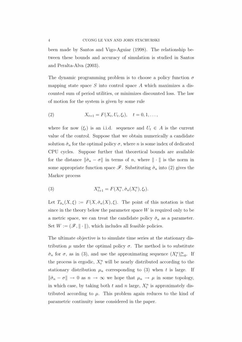
The dynamic programming problem is to choose a policy function σ

mapping state space S into control space A which maximizes a dis-

counted sum of period utilities, or minimizes discounted loss. The law

of motion for the system is given by some rule

(2) Xt+1 = F (Xt, Ut, ξt), t = 0, 1, . . . ,

where for now (ξt) is an i.i.d. sequence and Ut ∈ A is the current

value of the control. Suppose that we obtain numerically a candidate

solution σn for the optimal policy σ, where n is some index of dedicated

CPU cycles. Suppose further that theoretical bounds are available

for the distance ‖σn − σ‖ in terms of n, where ‖ · ‖ is the norm in

some appropriate function space F . Substituting σn into (2) gives the

Markov process

(3) Xnt+1 = F (Xn

t , σn(Xnt ), ξt).

Let Tσn(X, ξ) := F (X, σn(X), ξ). The point of this notation is that

since in the theory below the parameter space W is required only to be

a metric space, we can treat the candidate policy σn as a parameter.

Set W := (F , ‖ · ‖), which includes all feasible policies.

The ultimate objective is to simulate time series at the stationary dis-

tribution µ under the optimal policy σ. The method is to substitute

σn for σ, as in (3), and use the approximating sequence (Xnt )∞t=0. If

the process is ergodic, Xnt will be nearly distributed according to the

stationary distribution µn corresponding to (3) when t is large. If

‖σn − σ‖ → 0 as n → ∞ we hope that µn → µ in some topology,

in which case, by taking both t and n large, Xnt is approximately dis-

tributed according to µ. This problem again reduces to the kind of

parametric continuity issue considered in the paper.


2.3. The Solow-Phelps Stochastic Golden Rule. Next we con-

sider a more specific example, which is of independent interest, and

also helps to illustrate how one might verify the conditions we impose.

The example is the Solow-Phelps stochastic golden rule problem for a

one-sector economy. The framework is a Solow growth model, to which

a random component is added. The problem is to choose a savings rate

which maximizes expected utility of consumption at the steady state.

Surprisingly the existence of a solution to this problem has not been

treated to our knowledge.1

Since the savings rate takes values in compact set [0, 1], determining

existence of a solution reduces in effect to proving continuity of the

map from savings rate to stationary distribution.

In more detail, suppose initially a fixed savings rate s from current

income. At each period t production takes place, deriving from cap-

ital stock kt random output yt = f(kt) ξt; where f : S → S is the

production function, S := (0,∞), and ξt is a productivity shock with

distribution ν on S. The parameter is the savings rate, and we take

the parameter space W to be (0, 1]. Here s = 0 is excluded so as to

eliminate trivialities.

For simplicity, depreciation is taken to be total. Given savings rate s,

next period capital is

(4) kt+1 = s · f(kt) ξt.

The process then repeats, generating Markov chain (kt)∞t=0 starting

from k0 ∈ S given. In order that this process have a stationary distri-

bution, some restrictions on f and ν are necessary:

1Schenk-Hoppe (2002) considers maximization of expected consumption in a very

general stochastic environment. This is a direct generalization of the determinis-

tic problem. However in a stochastic setting maximization of expected utility of

consumption is perhaps the more natural criterion.


Assumption 2.1. The function f is continuously differentiable on S,

increasing, concave, and satisfies f(k) = 0 ⇐⇒ k = 0 and the Inada

conditions limk↓0 f′(k) = ∞, limk↑∞ f ′(k) = 0.

Assumption 2.2. Both E[ξt] and E[1/ξt] are finite. The Lebesgue

measure is absolutely continuous with respect to ν (non-Lebesgue-null

sets have positive ν-measure).

The restrictions on f are presented in the current form because they

are so familiar, but a quick reading of the proofs shows they are much

stronger than what is actually required. The assumptions E[ξt] < ∞and E[1/ξt] < ∞ restrict the right and left-hand tails of the shock

respectively.2 The assumption that ν is positive on sets of positive

Lebesgue measure—which is used to prove uniqueness—is also much

stronger than required, but simplifies the analysis, and holds for many

standard econometric shocks. For example, all lognormal distributions

satisfy the three restrictions in Assumption 2.2.

The golden rule problem is to maximize expected utility of consumption

at the steady state. Let u : [0,∞) → R be a utility function.

Assumption 2.3. The function u is continuous, bounded, strictly in-

creasing and, by adding or subtracting a constant if necessary, satisfies

u(0) = 0.

Suppose that for each savings rate s, (4) has a unique stationary dis-

tribution µs (for a precise definition of stationary distribution see Defi-

nition 3.2 below). Consumption ct is just (1−s)f(kt)ξt. Recalling that

kt and ξt are independent, the distribution of ct in equilibrium is

(5) ϕs(B) := Prob{ct ∈ B} =

∫ ∫1B[(1− s)f(k)z]ν(dz)µs(dk),

2With unbounded shocks some restrictions of this nature are necessary for the

stationary distribution to exist—the first restriction prevents unbounded growth;

the second collapse to the origin.


kt

kt+1 450

snf(kt)

sf(kt)

µsn

d→ µs

-

6

Figure 1. Convergence of stationary distributions.

where 1B[(1− s)f(k)z] = 1 when (1− s)f(k)z ∈ B and zero otherwise.

The golden rule problem is to select the “lottery” ϕs which maximizes

expected utility:

(6) max0≤s≤1

Esu(c), Esu(c) :=

∫u dϕs.

We now have the following result. All definitions are made precise

in Section 3. The proofs are in Section 4. Part 1 of Theorem 2.1 is

illustrated in Figure 1.

Theorem 2.1. Regarding the Solow–Phelps golden rule problem, let

Assumptions 2.1, 2.2 and 2.3 hold. The following statements are true.

1. For each savings rate s, the process (4) has a unique stationary

distribution, which depends continuously on s.

2. Moreover, an interior solution s∗ to the stochastic Phelps golden

rule problem (6) exists, at which the expected utility of long run

equilibrium consumption is maximized.

3. The General Model

In what follows, for measurable space (E,E ) let P(E) denote the prob-

abilistic measures on (E,E ), and bM (S) the finite signed measures.


Functional notation is often used for integration: if h : E → R is E -

measurable and µ ∈ bM (E) then µ(h) :=∫hdµ when the latter is

defined. If E has a topology, the σ-algebra E is always the Borel sets.

Throughout the paper we use the convention that if X is a random

variable taking values in measurable space (E,E ), then L(X) is the

law (distribution) of X, an element of P(E).

Let E have a topology, and let Cb(E) be the continuous bounded func-

tions on E. To each h ∈ Cb(E) there corresponds the linear func-

tional on bM (E) defined by µ 7→ µ(h) ∈ R. The weak topology

w(bM (E), Cb(E)) on bM (E) is the smallest topology which makes all

such functionals continuous. Also, w(P(E), Cb(E)) is the weak topol-

ogy on P(E) (i.e., the relative topology inhereted from bM (E)). For

a collection of probabilities {µn}∞n=1 ∪ {µ} ⊂ P(E), we write µnd→ µ

when the sequence (µn) converges to µ in w(P(E), Cb(E))—that is

when µn(h) → µ(h) in R for every h ∈ Cb(E). We say that (µn) con-

verges to µ in distribution (Stokey, Lucas and Prescott, 1989, Chapter

12).

3.1. The Model. Now let α ∈ W be a parameter. Consider an econ-

omy that evolves according to the rule

(7) Xt+1 = Tα(Xt, ξt), X0 ≡ x0 ∈ S given.

The sequence of shocks (ξt)∞t=0 is assumed to be uncorrelated and identi-

cally distributed.3 Together, the transition rule Tα and the distribution

of the shock—call it ν—determine a Markov chain (Xt)∞t=0. The tim-

ing is that Xt is observed at the start of time t, planning of economic

activity takes place on the basis of this information, and is then imple-

mented through the period. Implementation is perturbed by a shock

ξt, giving rise to Xt+1 at the start of the next period via (7). It is clear

from the timing that Xt and ξt are independent.

3As is well-known, correlations of finite order can be treated in this framework

by redefining state variables and, if necessary, adjusting the dimensions of the state

space.


The random variable Xt evolves in state space S. The state space has

a topology, and B(S) denotes the Borel sets of S. Also, let (Z,Z )

be any measurable space, with the shocks that perturb the economy in

each period taking values in Z, so that Tα : S×Z → S.4 The parameter

space W is any metric space.

3.2. Basic Assumptions. Some basic requirements are now given

which will at least assure the existence and uniqueness of stationary

distributions.

Assumption 3.1. The space S is separable and completely metrizable.

Such spaces are called Polish. For example, in the golden rule problem

the state space is S = (0,∞) with the usual topology. This space is

Polish. In fact every open (indeed, every Gδ) subset of a complete

metric space is completely metrizable by Alexandrov’s Lemma (c.f.,

e.g., Aliprantis and Border, 1999, Theorem 3.22).

Assumption 3.2. For each fixed α ∈ W , x 7→∫h[Tα(x, z)]ν(dz) is

continuous and bounded whenever h : S → R is.

While it may not immediately appear so, this assumption is easy to

verify in applications. For example, it holds when x 7→ Tα(x, z) is con-

tinuous for each fixed α and z, as follows from Dominated Convergence.

The continuity provided by Assumption 3.2 is paired with a compact-

ness requirement below to obtain existence of stationary distributions

via a fixed point argument. To define the compactness requirement,

first we introduce norm-like functions, which play a role somewhat

analogous to Liapunov functions in dynamical systems theory.

Definition 3.1. A continuous function V : S → [0,∞) is called norm-

like if there is an increasing sequence of compact sets (Kj)∞j=1 with

∪∞j=1Kj = S and infx/∈KjV (x) →∞ as j →∞.

4Of course Tα is required to be (B(S)⊗Z ,B(S))-measurable, ∀α ∈ W .


L(Xt) L(Xt+1)

V? ?

Figure 2. A norm-like function on (0,∞).

A norm-like function V gets larger and larger at the “edges” of the

state space, so we can be sure that L(Xt) stays near the “center” of

the space by checking that the expectation of V (Xt) is bounded in t

(Figure 2). The next condition will guarantee precisely this. It means

that there is on average a drift of the state variable towards parts of

the state space on which V is remains small.

Assumption 3.3. For each α ∈ W , there exists a norm-like function

V and constants λ, b ∈ [0,∞) with λ < 1 and

(8)

∫V [Tα(x, z)]ν(dz) ≤ λV (x) + b, ∀x ∈ S.

Finally, the question of parametric continuity of stationary distribu-

tions is most interesting when this distribution is unique (for each pa-

rameterization). Fortunately, uniqueness is far more common in sto-

chastic models than in deterministic ones, as a result of the mixing pro-

vided by noise. In order to generate uniqueness we assume throughout

the paper the following, although any other uniqueness condition will

do.

Assumption 3.4. For each α ∈ W , the process (7) is ψ-irreducible. In

other words, there is a ψ ∈ P(S), possibly depending on the parameter


α, such that ψ(B) > 0 implies

Probx{Xt ∈ B for some t ∈ N} > 0, ∀x ∈ S,

where Probx is the distribution of (Xt)∞t=0 when X0 ≡ x.

Again, this assumption is often easier to verify in practice than it looks.

See the proof for the golden rule example below.

3.3. Stationary Distributions. Conditions for the existence of sta-

tionary distributions for Markov processes on uncountable state space

have been investigated by many authors. In economics, a well known

result is that Feller processes on compact state space have at least one

stationary distribution (Stokey, Lucas and Prescott, 1989, Theorem

12.10). The compactness requirement can be weakened to the condi-

tion that at least one “trajectory” of the process (7) be precompact.

Intuitively, if this is the case then up to an epsilon, probability mass

stays in a compact set at least for one starting point—by Prohorov’s

theorem, see below—and the compact state proof can be generalized

appropriately. The details follow.

The long run equilibrium of the economy (7) is identified—when it

exists—with the stationary distribution µα of the Markov chain (Xt) =

(Xαt ).

Definition 3.2. Distribution µα ∈ P(S) is called stationary for (7) if

(9) µα(B) =

∫S

[∫Z

1B[Tα(x, z)]ν(dz)

]µα(dx), ∀B ∈ B(S).

Here 1B[Tα(x, z)] = 1 if Tα(x, z) ∈ B and zero otherwise, so the inner

integral has the interpretation Prob{Xt+1 ∈ B |Xt = x}. Equation (9)

states that if L(Xt) = µα, then so does L(Xt+1).


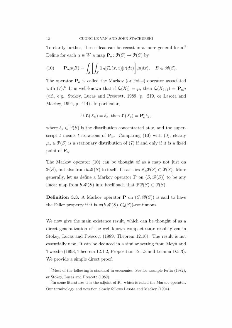
To clarify further, these ideas can be recast in a more general form.5

Define for each α ∈ W a map Pα : P(S) → P(S) by

(10) Pαµ(B) =

∫S

[∫Z

1B[Tα(x, z)]ν(dz)

]µ(dx), B ∈ B(S).

The operator Pα is called the Markov (or Foias) operator associated

with (7).6 It is well-known that if L(Xt) = µ, then L(Xt+1) = Pαµ

(c.f., e.g. Stokey, Lucas and Prescott, 1989, p. 219, or Lasota and

Mackey, 1994, p. 414). In particular,

if L(X0) = δx, then L(Xt) = Ptαδx,

where δx ∈ P(S) is the distribution concentrated at x, and the super-

script t means t iterations of Pα. Comparing (10) with (9), clearly

µα ∈ P(S) is a stationary distribution of (7) if and only if it is a fixed

point of Pα.

The Markov operator (10) can be thought of as a map not just on

P(S), but also from bM (S) to itself. It satisfies PαP(S) ⊂ P(S). More

generally, let us define a Markov operator P on (S,B(S)) to be any

linear map from bM (S) into itself such that PP(S) ⊂ P(S).

Definition 3.3. A Markov operator P on (S,B(S)) is said to have

the Feller property if it is w(bM (S), Cb(S))-continuous.

We now give the main existence result, which can be thought of as a

direct generalization of the well-known compact state result given in

Stokey, Lucas and Prescott (1989, Theorem 12.10). The result is not

essentially new. It can be deduced in a similar setting from Meyn and

Tweedie (1993, Theorem 12.1.2, Proposition 12.1.3 and Lemma D.5.3).

We provide a simple direct proof.

5Most of the following is standard in economics. See for example Futia (1982),

or Stokey, Lucas and Prescott (1989).6In some literatures it is the adjoint of Pα which is called the Markov operator.

Our terminology and notation closely follows Lasota and Mackey (1994).


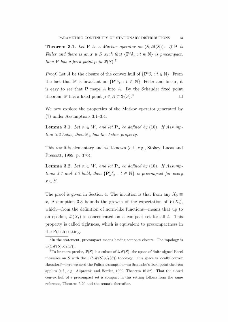
Theorem 3.1. Let P be a Markov operator on (S,B(S)). If P is

Feller and there is an x ∈ S such that {Ptδx : t ∈ N} is precompact,

then P has a fixed point µ in P(S).7

Proof. Let A be the closure of the convex hull of {Ptδx : t ∈ N}. From

the fact that P is invariant on {Ptδx : t ∈ N}, Feller and linear, it

is easy to see that P maps A into A. By the Schauder fixed point

theorem, P has a fixed point µ ∈ A ⊂ P(S).8 �

We now explore the properties of the Markov operator generated by

(7) under Assumptions 3.1–3.4.

Lemma 3.1. Let α ∈ W , and let Pα be defined by (10). If Assump-

tion 3.2 holds, then Pα has the Feller property.

This result is elementary and well-known (c.f., e.g., Stokey, Lucas and

Prescott, 1989, p. 376).

Lemma 3.2. Let α ∈ W , and let Pα be defined by (10). If Assump-

tions 3.1 and 3.3 hold, then {Ptαδx : t ∈ N} is precompact for every

x ∈ S.

The proof is given in Section 4. The intuition is that from any X0 ≡x, Assumption 3.3 bounds the growth of the expectation of V (Xt),

which—from the definition of norm-like functions—means that up to

an epsilon, L(Xt) is concentrated on a compact set for all t. This

property is called tightness, which is equivalent to precompactness in

the Polish setting.

7In the statement, precompact means having compact closure. The topology is

w(bM (S), Cb(S)).8To be more precise, P(S) is a subset of bM (S), the space of finite signed Borel

measures on S with the w(bM (S), Cb(S)) topology. This space is locally convex

Hausdorff—here we need the Polish assumption—so Schauder’s fixed point theorem

applies (c.f., e.g. Aliprantis and Border, 1999, Theorem 16.52). That the closed

convex hull of a precompact set is compact in this setting follows from the same

reference, Theorem 5.20 and the remark thereafter.


We now collect these results and combine them with Assumption 3.4

to obtain existence and uniqueness.

Theorem 3.2. If Assumptions 3.1–3.4 hold, then the Markov chain

(7) has a unique stationary distribution µα for each α ∈ W .

Proof. Existence follows from Theorem 3.1 and Lemmas 3.1 and 3.2.

Uniqueness under Assumption 3.4 is well-known. See, for example,

Meyn and Tweedie (1993, Theorem 10.0.1 and Proposition 10.1.1). �

3.4. Parametric Continuity. We can now progress to the main re-

sults of the paper, concerning parametric continuity of stationary distri-

butions. First, though, in order to have any hope of getting parametric

continuity in the stationary distributions, we at least need continuity

in the primitives:

Assumption 3.5. The transition rule Tα is continuous in α. That is,

α 7→ Tα(x, z) is continuous for each x ∈ S and z ∈ Z.

Two different parametric continuity results will be presented. The

first requires two additional conditions. Specifically, we strengthen

Assumptions 3.2 and 3.3 to hold in a uniform way over the parameters.

In the statement of the theorem, % is any metric compatible with the

topology on S.

Theorem 3.3. Let Assumptions 3.1–3.5 hold, and let {αn}∞n=1∪{α} ⊂W . Suppose that for each compact K ⊂ S, there is a constant M <∞which can be chosen independent of αn to satisfy

(11)

∫%[Tαn(x, z), Tαn(x′, z)]ν(dz) ≤M%(x, x′) whenever x, x′ ∈ K.

Suppose further that V , λ and b in Assumption 3.3 can be chosen in-

dependent of αn. Let µαn and µα in P(S) be the unique stationary

distributions of (7) for each αn and α respectively. In this case, if

αn → α, then µαn

d→ µα.


The proof is in Section 4. The condition (11) requires that the model

(7) satisfy a local Lipschitz condition “on average,” where the Lips-

chitz constant can be chosen independent of the points in the sequence

αn. For an example of how to check this and the other hypotheses of

Theorem 3.3, see the proof of Theorem 2.1 (the golden rule problem)

in Section 4.

The second result (Theorem 3.4, below) depends on various order prop-

erties, which replace the uniform continuity and uniform boundedness

assumptions in Theorem 3.3. In particular, the set of stationary dis-

tributions may form a (stochastic dominance) order interval in P(S).

These order intervals are compact in the topology of weak convergence

for certain spaces S. The compactness of this set can substitute in

some sense for the compactness of the state space assumed in earlier

results.

A number of order concepts are introduced.9 Recall that a relation

≤E on a space E is called an order if it is reflexive, transitive and

antisymmetric. If (X,≤X) and (E,≤E) are two ordered spaces, a map

T : X → E is called increasing if Tx ≤E Tx′ whenever x ≤X x′,

decreasing if Tx′ ≤E Tx whenever x ≤X x′, and monotone if it is

either increasing or decreasing. A subset of (E,≤E) is called increasing

(decreasing) if its indicator function is an increasing (a decreasing)

function (into R with the usual order). Given A ⊂ E, i(A) is the

smallest increasing set containingA, and d(A) is the smallest decreasing

set. If (E,E ) is a measure space with order ≤E, then ibE denotes the

increasing bounded E -measurable real functions on E.

When E has a topology, ≤E is called separating if, whenever x �E y,

there is an increasing continuous bounded h : E → R with h(x) > h(y).

For example, Rn with the usual topology and order is separating.

9For more details we refer to the excellent survey of Torres (1990).


If E is metrizable with separating order ≤E, then ≤E induces on P(E)

the order ≤P(E) of stochastic dominance.10 It is defined by

µ ≤P(E) µ′ iff µ(h) ≤ µ′(h), ∀h ∈ ibE , E the Borel sets.

In what follows let the state space S and the parameter space W be

given orders ≤S and ≤W respectively. We require some restrictions on

the order ≤S and its interaction with the topology of S:

Assumption 3.6. The order ≤S on S is separating. In addition, if K

is a compact subset of S, then i(K) ∩ d(K) is again compact in S.11

For example, Assumption 3.6 holds on the space Rn with the usual

order and topology.

We have the following preliminary result, which extends Hopenhahn

and Prescott (1992, Corollary 3) to a noncompact setting. The proof

uses a result of Huggett (2003) on monotone comparative dynamics,

a convergence result of Meyn and Tweedie (1993), and the fact that

separating orders are closed.

Proposition 3.1. Let Assumptions 3.1—3.6 hold. Suppose further

that for fixed α ∈ W and z ∈ Z, x 7→ Tα(x, z) is increasing, and for

fixed x ∈ S and z ∈ Z, α 7→ Tα(x, z) is increasing. Let α, β ∈ W ,

and let µα and µβ be the corresponding stationary distributions. In this

case, if α ≤W β, then µα ≤P(S) µβ.

In other words, the stationary distribution is (stochastic dominance)-

increasing in the parameter. The second parametric continuity result

is as follows.

10Without some restrictions on the topology and order ≤E , the induced relation

≤P(E) may not be antisymmetric. (See Torres, 1990, Theorem 5.3.)11This last condition is used in Torres (1990, p 33) to generate w(P(S), Cb(S))-

compact ≤P(S)-order intervals in P(S).


Theorem 3.4. Let the hypotheses of Proposition 3.1 hold, and let

{αn}∞n=1 ∪ {α} ⊂ W . Let µαn and µα in P(S) be the unique station-

ary distributions of (7) for each αn and α respectively. In this case, if

αn → α monotonically in W , then µαn

d→ µα.

The conditions (i) x 7→ Tα(x, z) increasing for fixed α ∈ W and z ∈ Z,

and (ii) α 7→ Tα(x, z) increasing for fixed x ∈ S and z ∈ Z hold

for many economic models. For example, the transition rule for the

stochastic optimal growth model is well-known to be increasing in the

state variable (c.f., e.g., Hopenhayn and Prescott, 1992). Also, the

transion rule is increasing in the discount factor (a parameter) for each

value of the state and shock (c.f., e.g., Danthine and Donaldson, 1981).

Corollary 3.1. If, in addition, W ⊂ R, then the conclusion holds even

when the sequence (αn)∞n=1 is not monotone.

Proof. Write µn for µαn and µ for µα. Sinced→ is convergence in a topol-

ogy, it is sufficient to show that every subsequence (µn(k))∞k=1 of µn has

a subsubsequence (µn(k(j)))∞j=1 converging to µ. So pick any (µn(k))

∞k=1.

Since every sequence in R has a monotone subsequence, and since ev-

ery subsequence of (αn)∞n=1 converges to α, there is a subsequence of

(αn(k))∞k=1—call it (αn(k(j)))

∞j=1—which converges monotonically to α.

In which case µn(k(j))d→ µ by Theorem 3.4, completing the proof. �

4. Proofs

4.1. The Golden Rule Problem. First we give the proof of Theo-

rem 2.1 based on the parametric continuity results in Section 3. The

proof is based on Theorem 3.3. (Alternatively, the same results can

be established through Corollary 3.1.) The hypotheses of Theorem 3.3

are now progressively verified.

That Assumption 3.1 holds for S = (0,∞) was verified after the state-

ment of the assumption. Assumption 3.2 is immediate from the Dom-

inated Convergence Theorem and continuity of f : For all s ∈ W :=


(0, 1] and h ∈ Cb(S),∫h[sf(kn)z]ν(dz) →

∫h[sf(k)z]ν(dz) whenever kn → k ∈ S.

Regarding Assumption 3.3, pick any s ∈ W . On S = (0,∞) let V (k) :=

k+k−1. Clearly V is norm-like on S. By Assumption 2.2, we can choose

a real number γ strictly larger than E(1/ξ). By the Inada conditions

and differentiability there is a δ > 0 such that sf(k) ≥ γk on (0, δ),

and then a c > 0 such that sf(k) ≥ c on [δ,∞) by monotonicity, in

which case1

sf(k)≤ 1

γk+

1

cfor all k in (0,∞).

In addition, by the diminishing returns Inada condition, concavity and

the finite mean of the shock, there is an a1 < 1 and b1 <∞ such that

sf(k)Eξ ≤ a1k + b1, ∀k. From these bounds we get∫V [sf(k)z]ν(dz) =

∫sf(k)zν(dz) +

∫1

sf(k)zν(dz)

≤ a1k + b1 +E(1/ξ)

γk+

E(1/ξ)

c.

Setting λ := a1 ∨ [E(1/ξ)/γ] < 1 and b := b1 + [E(1/ξ)/c] gives (8).

Regarding Assumption 3.4, fix s ∈ (0, 1] =: W and let ψ be any proba-

bility on (0,∞) with a density. Now take any B ⊂ (0,∞) with positive

ψ-measure and any k ∈ (0,∞) =: S. It is easy to check that the set

B/sf(k) has positive Lebesgue measure, so that from Assumption 2.2

we have

Probk{kt ∈ B for some t ∈ N} ≥ Probk{k1 ∈ B}

= ν{z : sf(k)z ∈ B} = ν[B/sf(k)] > 0.

Here Probk is the distribution of (kt)∞t=0 when k0 ≡ k.

From Theorem 3.1 we now already know that (kt)∞t=0 has a unique

stationary distribution. For Theorem 3.3 to hold, however, there are

some additional conditions. Let {sn}∞n=1 ∪ {s} ⊂ W . First, pick any

compact K ⊂ S = (0,∞). Since f is continuously differentiable, there


is a number A such that |f(k) − f(k′)| ≤ A|k − k′| for all k, k′ ∈ K.

But then∫|snf(k)z − snf(k′)z|ν(dz) ≤

∫zν(dz)|f(k)− f(k′)|

≤∫zν(dz)A|k − k′|.

Thus M :=∫zν(dz)A verifies the bound in (11) independent of the

value sn.

To finish checking the hypotheses of Theorem 3.3, it remains only to

verify that V , λ and b in Assumption 3.3 can be chosen independent

of sn. Let V (k) = 1/k + k as before. By restricting attention to the

tail of the sequence (sn) if necessary we can assume that r := infn sn >

0, because sn → s ∈ W = (0, 1]. As above, we can choose a real

number γ strictly larger than E(1/ξ). By the Inada conditions and

differentiability there is a δ > 0 such that rf(k) ≥ γk on (0, δ), and

then a c > 0 such that rf(k) ≥ c on [δ,∞) by monotonicity, in which

case

1

snf(k)≤ 1

rf(k)≤ 1

γk+

1

c∀n ∈ N, ∀ k ∈ (0,∞).

In addition, by the diminishing returns Inada condition, concavity and

the finite mean of the shock, there is an a1 < 1 and b1 <∞ such that

snf(k)Eξ ≤ f(k)Eξ ≤ a1k + b1, ∀k. From these bounds we get∫V (snf(k)z)ν(dz) =

∫snf(k)zν(dz) +

∫1

snf(k)zν(dz)

≤ a1k + b1 +E(1/ξ)

γk+

E(1/ξ)

c.

Setting λ := a1 ∨ [E(1/ξ)/γ] < 1 and b := b1 + [E(1/ξ)/c] gives (8).

We have now verified all the hypotheses of Theorem 3.3, and hence

established Part 1 of Theorem 2.1.

Regarding Part 2, we first establish continuity of the objective func-

tion (6). Take any s ∈ W . Let µ(s) be the corresponding stationary


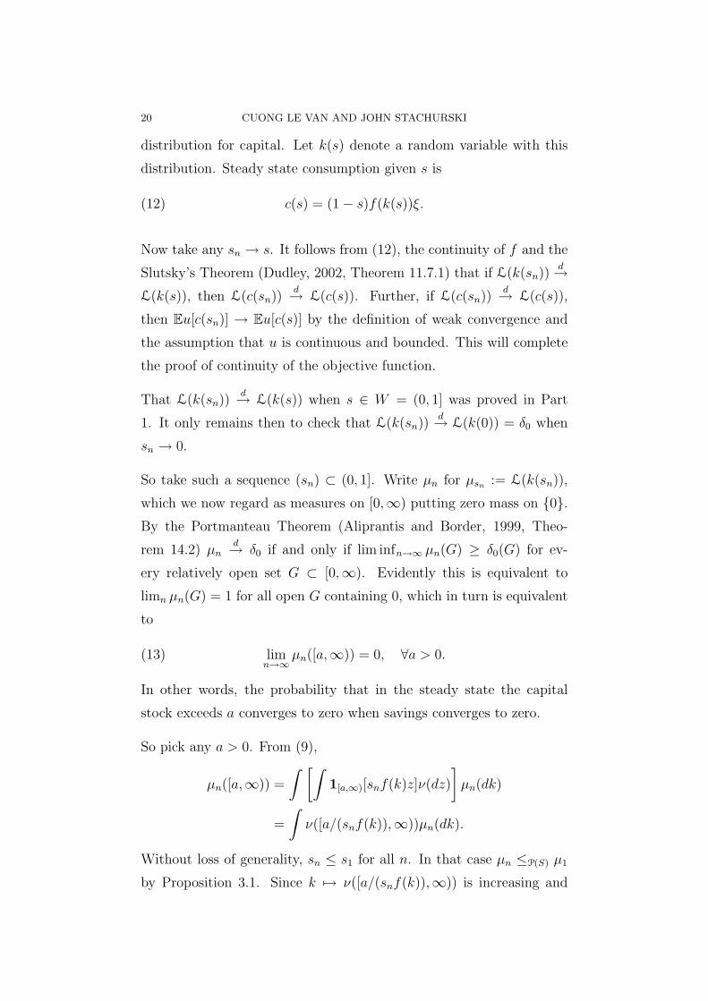
distribution for capital. Let k(s) denote a random variable with this

distribution. Steady state consumption given s is

(12) c(s) = (1− s)f(k(s))ξ.

Now take any sn → s. It follows from (12), the continuity of f and the

Slutsky’s Theorem (Dudley, 2002, Theorem 11.7.1) that if L(k(sn))d→

L(k(s)), then L(c(sn))d→ L(c(s)). Further, if L(c(sn))

d→ L(c(s)),

then Eu[c(sn)] → Eu[c(s)] by the definition of weak convergence and

the assumption that u is continuous and bounded. This will complete

the proof of continuity of the objective function.

That L(k(sn))d→ L(k(s)) when s ∈ W = (0, 1] was proved in Part

1. It only remains then to check that L(k(sn))d→ L(k(0)) = δ0 when

sn → 0.

So take such a sequence (sn) ⊂ (0, 1]. Write µn for µsn := L(k(sn)),

which we now regard as measures on [0,∞) putting zero mass on {0}.By the Portmanteau Theorem (Aliprantis and Border, 1999, Theo-

rem 14.2) µnd→ δ0 if and only if lim infn→∞ µn(G) ≥ δ0(G) for ev-

ery relatively open set G ⊂ [0,∞). Evidently this is equivalent to

limn µn(G) = 1 for all open G containing 0, which in turn is equivalent

to

(13) limn→∞

µn([a,∞)) = 0, ∀a > 0.

In other words, the probability that in the steady state the capital

stock exceeds a converges to zero when savings converges to zero.

So pick any a > 0. From (9),

µn([a,∞)) =

∫ [∫1[a,∞)[snf(k)z]ν(dz)

]µn(dk)

=

∫ν([a/(snf(k)),∞))µn(dk).

Without loss of generality, sn ≤ s1 for all n. In that case µn ≤P(S) µ1

by Proposition 3.1. Since k 7→ ν([a/(snf(k)),∞)) is increasing and


bounded, by the definition of stochastic dominance

(14) µn([a,∞)) ≤∫ν([a/(snf(k)),∞))µ1(dk).

In addition, limn→∞ ν([a/(snf(k)),∞)) = 0 by Dominated Conver-

gence, so applying Dominated Convergence to (14) gives (13) as re-

quired.

We conclude that the objective function (6) is continuous for s ∈ [0, 1],

a compact set. Therefore a solution to the golden rule problem exists.

That it is interior is immediate from (12), since u is strictly positive on

(0,∞) and integrals of strictly positive functions are strictly positive.

(Therefore s = 0 and s = 1 are not solutions, as in both cases the value

of the objective function is zero.)

4.2. Remaining Proofs. We first give some general discussion.

It is known that when S is Polish, P(S) with topology w(P(S), Cb(S))

is itself Polish, completely metrized by the Fortet-Mourier metric de-

scribed below. Let BL(S, %) be the collection of bounded Lipschitz

functions on (S, %). This space is given the norm

(15) ‖h‖BL := supx∈S

|h(x)|+ supx 6=y

|h(x)− h(y)|%(x, y)

.

Now set dFM(µ, ν) := sup |µ(h) − ν(h)|, where the supremum is over

all h ∈ BL(S, %), ‖h‖BL ≤ 1. Then dFM metrizes w(P(S), Cb(S)) (c.f.,

e.g., Dudley 2002, Theorem 11.3.3).

As usual, we say that

Definition 4.1. A collection P0 ⊂ P(S) is tight if, for every ε > 0,

there is a compact set K ⊂ S such that supµ∈P0µ(S \ K) < ε. Also,

P0 ⊂ P(S) is called precompact if it has compact closure.

We will make extensive use of Prohorov’s Theorem (c.f., e.g., Aliprantis

and Border, 1999, Theorem 14.22): For S Polish and P(S) with the

w(P(S), Cb(S)) topology, a subset of P(S) is tight if and only if it is

precompact.


Proof of Lemma 3.2. Fix α ∈ W . By Meyn and Tweedie (1993, Lemma

D.5.3), a set P0 ⊂ P(S) is tight if (and only if) there is a norm-like func-

tion V such that supµ∈P0µ(V ) <∞. This is true for P0 = {Pt

αδx}∞t=1,

because if V , λ and b are as in Assumption 3.3, then

Ptαδx(V ) = PαP

t−1α δx(V )

=

∫S

[∫Z

V [Tα(u, z)]ν(dz)

]Pt−1

α δx(du).

(Substitute Pt−1α δx for µ and V for 1B in (10).) But∫

S

[∫Z

V [Tα(u, z)]ν(dz)

]Pt−1

α δx(du)

≤∫

S

[λV (u) + b]Pt−1α δx(du) = λPt−1

α δx(V ) + b.

Repeating this argument t times gives

(16) Ptαδx(V ) ≤ λtV (x) +

b

1− λ≤ V (x) +

b

1− λ.

∴ supt∈N

Ptαδx(V ) <∞.

Thus {Ptαδx}∞t=1 is tight, and hence precompact by Prohorov’s Theo-

rem. �

In order to prove Theorems 3.3–3.4 and Proposition 3.1 we will make

use of the following lemma.

Lemma 4.1. Fix β ∈ W . Under Assumptions 3.1—3.4, not only does

Pβ have a unique fixed point µβ ∈ P(S), but in addition the averages

of the marginal distributions converge to it in distribution. That is,

(17)1

t

t∑j=1

Pjβδx

d→ µβ, ∀x ∈ S.

Proof. Immediate from Lemma 3.2, Theorem 3.2 and Meyn and Tweedie

(1993, Theorem 12.1.4). �

Proof of Theorem 3.3. For arbitrary β ∈ W , we know by Theorem 3.2

that the process (Xt)∞t=0 = (Xβ

t )∞t=0 has a unique stationary distribu-

tion. In other words, Pβ has a unique fixed point µβ ∈ P(S). Let (αn)


and α be as in the statement of the theorem. In what follows, write µn

for µαn , µ for µα, and analogously for Tαn , Tα and so on.

We first claim that the set of stationary distributions {µn}∞n=1 is pre-

compact in w(P(S), Cb(S)). To see this, note that for every x ∈ S,

(i) Px := {Ptnδx : t, n ∈ N} is a tight subset of P(S); and (ii) so is

Qx := {1t

∑tj=1 Pj

nδx : t, n ∈ N}. The reason for (i) is as follows. By

hypothesis, the function V and constants λ and b on the right hand

side of (16) can be chosen independent of αn (as well as t), so that

supt,n Pjnδx(V ) < ∞. This implies tightness as discussed in the proof

of Lemma 3.2. From (i), (ii) is immediate. By Prohorov’s theorem,

tightness of Qx implies precompactness. Finally, note that {µn}∞n=1 is

in the closure of Qx for some fixed x ∈ S by (17). The claim follows.

As a result, every subsequence of (µn) has a convergent subsubsequence,

written here as (µj). Denote the limit of (µj) by µ0. Suppose we can

show for this arbitrary subsequence that the limit point µ0 is equal

to µ. In this case every subsequence of (µn) has a subsubsequence

converging to µ, and—since convergence in distribution is convergence

in a topology—it must be that the sequence (µn) itself converges to µ,

which is what we wish to prove.

So let (µj) be the above subsubsequence, µjd→ µ0. Pick any h ∈

BL(S, %), ‖h‖BL ≤ 1. Fix ε > 0. We have |Pµ0(h)−µ0(h)| dominated

by

|Pµ0(h)−Pµj(h)|+ |Pµj(h)− µj(h)|+ |µj(h)− µ0(h)|.

(18) ∴ |Pµ0(h)− µ0(h)| ≤ |Pµj(h)− µj(h)|+ ε, j large,

where we have used Lemma 3.1. Now consider the remaining term. We

have

|Pµj(h)− µj(h)| = |Pµj(h)−Pjµj(h)|

≤∫ ∣∣∣∣∫ h(Tj(x, z))ν(dz)−

∫h(T (x, z))ν(dz)

∣∣∣∣µj(dx).


(Substitute h for 1B in (10).) Since {µn} and hence {µj} is precompact

it is tight, and there is a compact K ⊂ S with supj µj(S \ K) < ε.

Define real functions gj and g on K by

gj(x) :=

∫h[Tj(x, z)]ν(dz), g(x) :=

∫h[T (x, z)]ν(dz).

It follows from Assumption 3.5 and Dominated Convergence that gj

converges to g pointwise on K. Also, {gj : j ∈ N} as a collection of

real functions is uniformly bounded by 1 and uniformly equicontinuous,

as, for any x, x′ ∈ K,

|gj(x)− gj(x′)| ≤

∫|h(Tj(x, z))− h(T (x′, z))|ν(dz)

≤∫%[Tj(x, z), Tj(x

′, z)]ν(dz) (∵ ‖h‖BL ≤ 1)

≤M%(x, x′).

From the Arzela-Ascoli Theorem, {gj} is precompact in the supremum

norm topology, and therefore has a uniformly convergent subsequence.

Obviously the limit of this subsequence is g, so that, for some j ∈ N,

|gj(x)− g(x)| ≤ ε for all x ∈ K. But

|Pµj(h)−Pjµj(h)| ≤∫

K

|gj(x)− g(x)|µj(dx)

+

∫S\K

[∫|h(Tj(x, z))− h(T (x′, z))|ν(dz)

]µj(dx) ≤ ε+ 2ε.

Combining this with (18) gives

|Pµ0(h)− µ0(h)| < 4ε, ∀ε > 0.

∴ |Pµ0(h)− µ0(h)| = 0, ∀h ∈ BL(S, %), ‖h‖BL ≤ 1.

∴ sup{|Pµ0(h)− µ0(h)| : ‖h‖BL ≤ 1} = dFM(Pµ0, µ0) = 0.

∴ Pµ0 = µ0 (∵ dFM a metric).

Since P has only one fixed point in P(S), we conclude that µ0 = µ.

This completes the proof. �


Proof of Proposition 3.1. Let α and β be as in the statement of the

proposition. Pick any x ∈ S. Consider the Markov chains (Xαt )∞t=0 and

(Xβt )∞t=0 when Xα

0 = Xβ0 ≡ x. From Huggett (2003, Theorem 2) we

have

(19) L(Xαt ) = Pt

αδx ≤P(S) Ptβδx = L(Xβ

t ), ∀t ∈ N

whenever the following two conditions hold:

(i) x ≤S x′ implies Pγδx ≤P(S) Pγδx′ , all γ ∈ W .

(ii) α ≤W β implies Pαδx ≤P(S) Pβδx, all x ∈ S.

Both of these are easy to verify from the hypotheses of the proposition.

∴1

t

t∑j=1

Pjαδx ≤P(S)

1

t

t∑j=1

Pjβδx ∀t ∈ N0.

Taking limits with respect to t now gives µα ≤P(S) µβ, where we have

used (17) and the fact that ≤P(S) is a w(P(S), Cb(S))-closed order on

P(S) (Assumption 3.6—separating implies closed—and Torres, 1990,

Theorem 6.1). �

Proof of Theorem 3.4. Once again, for each β ∈ W , Pβ has a unique

fixed point and (17) holds. Take (αn) monotone and converging to α ∈W . We can and do assume that the sequence is increasing: αn ↑ α.12

As before we write µn for µαn , µ for µα, and analogously for Tαn , Tα

and so on.

The first important observation is that By Proposition 3.1,

µ1 ≤P(S) µn ≤P(S) µ, ∀n ∈ N.

Moreover, in the present setting and order intervals are compact (As-

sumption 3.6 and Torres ,1990, Theorem 6.6). Indeed, it follows from

Assumption 3.6, and Torres (1990, Proposition 6.7) that µnd→ µ0 for

some µ0 ∈ P(S). If we can show that µ0 = µ then the proof is done.

12Otherwise define another order ≤′ on W by α ≤′ β iff β ≤W α.


From Assumption 3.6 and Torres (1990, Proposition 6.2), the increasing

functions in Cb(S) separate P(S), in the sense that if µ′ and µ′′ are

distinct elements of P(S), then there is an h ∈ ibB(S) ∩ Cb(S) with

µ′(h) 6= µ′′(h). Given that µ is the only fixed point of P, then, it

suffices to show that

(20) Pµ0(h) = µ0(h), ∀h ∈ ibB(S) ∩ Cb(S).

So take h ∈ ibB(S)∩Cb(S) and ε > 0. As in the proof of Theorem 3.3,

|Pµ0(h)− µ0(h)| is dominated by

|Pµ0(h)−Pµn(h)|+ |Pµn(h)− µn(h)|+ |µn(h)− µ0(h)|.

(21) ∴ |Pµ0(h)− µ0(h)| ≤ |Pµn(h)− µn(h)|+ ε, n large,

using Lemma 3.1. Consider the remaining term. We have

|Pµn(h)− µn(h)| = |Pµn(h)−Pnµn(h)|

≤∫ ∣∣∣∣∫ h(Tn(x, z))ν(dz)−

∫h(T (x, z))ν(dz)

∣∣∣∣µn(dx).

(Substitute h for 1B in (10).) Since {µn} is precompact by Prohorov’s

theorem it is tight, so there is a compact K ⊂ S with supn µn(S \K) <

ε. Define real functions gn and g on K by

gn(x) :=

∫h[Tn(x, z)]ν(dz), g(x) :=

∫h[T (x, z)]ν(dz).

It follows from Assumption 3.5 and Dominated Convergence that gn

converges to g pointwise on K. Since h is increasing, the pointwise

convergence is monotone. Since h ∈ Cb(S) and Assumption 3.2 holds,

gn and g are continuous. From Dini’s Lemma, then, gn also converges

uniformly to g on K, so that, for some n ∈ N, |gn(x) − g(x)| ≤ ε for

all x ∈ K. But then

|Pµn(h)−Pnµn(h)| ≤∫

K

|gn(x)− g(x)|µn(dx)

+

∫S\K

[∫|h(Tn(x, z))− h(T (x′, z))|ν(dz)

]µn(dx) ≤ ε+ 2Bε,


where B := supx∈S |h(x)|. Combining this with (21) gives

|Pµ0(h)− µ0(h)| < (2 + 2B)ε.

This verifies (20), which completes the proof. �

References

[1] Aliprantis, C. D. and K. C. Border (1999): Infinite Dimensional Analysis,

Second Edition, Springer-Verlag, New York.

[2] Danthine, J-P. and J. B. Donaldson (1981): Stochastic Properties of Fast vs.

Slow Growth Economies, Econometrica, 49 (4), 1007–1033.

[3] Dudley, R. M. (2002): Real Analysis and Probability, Cambridge Studies in

Advanced Mathematics No. 74, Cambridge University Press.

[4] Duffie, D. and K. J. Singleton (1993): “Simulated Moments Estimation of

Markov Models of Asset Prices,” Econometrica, 61 (4) 929–952.

[5] Futia, C. A. (1982): “Invariant Distributions and the Limiting Behavior of

Markovian Economic Models,” Econometrica, 50, 377–408.

[6] Hopenhayn, H. A. and E. C. Prescott (1992): “Stochastic Monotonicity and

Stationary Distributions for Dynamic Economies,” Econometrica, 60, 1387–

1406.

[7] Huggett, M. (2003): “When are comparative dynamics monotone?” Review of

Economic Dynamics, 6 (1), 1–11.

[8] Lasota, A. and M. C. Mackey (1994): Chaos, Fractals and Noise: Stochastic

Aspects of Dynamics, 2nd edition, Springer-Verlag, New York.

[9] Meyn, S. P. and Tweedie, R. L. (1993): Markov Chains and Stochastic Stabil-

ity, Springer-Verlag: London.

[10] Phelps, E.S. (1961): “The Golden Rule of Accumulation: A Fable for Growth-

men,” American Economic Review, 51, 638–643

[11] Santos, M. S. and A. Peralta-Alva (2003): “Accuracy of Simulations for Sto-

chastic Dynamic Models.” Manuscript.

[12] Santos, M. and Vigo-Aguiar J. T. (1998): “Analysis of a Numerical Dynamic

Programming Algorithm Applied to Economic Models,” Econometrica, 66, 2,

409–426.

[13] Schenk-Hoppe, K. R (2002): “Is There a Golden Rule for the Stochastic Solow

Growth Model?” Macroeconomic Dynamics 6, 457–475.

[14] Stokey, N. L., R. E. Lucas and E. C. Prescott (1989): Recursive Methods in

Economic Dynamics Harvard University Press, Massachusetts.


[15] Torres, R. (1990): “Stochastic Dominance.” DP n. 905, September 1990, Cen-

ter for Mathematical Studies in Economics and Management Science, North-

western University

Center for Operations Research and Econometrics, Universite Catholique

de Louvain, 34 Voie du Roman Pays, B-1348 Louvain-la-Neuve, Belgium

the university of melbourne - fbe.unimelb.edu.au€¦ · stokey, lucas and prescott for markov...

Documents