the university of chicago - pelagicos · the university of chicago the statistics and biology of...

The University of Chicago

The Statistics and Biology of the Species-Area RelationshipAuthor(s): Edward F. Connor and Earl D. McCoyReviewed work(s):Source: The American Naturalist, Vol. 113, No. 6 (Jun., 1979), pp. 791-833Published by: The University of Chicago Press for The American Society of NaturalistsStable URL: http://www.jstor.org/stable/2460305 .Accessed: 19/09/2012 21:23

Your use of the JSTOR archive indicates your acceptance of the Terms & Conditions of Use, available at .http://www.jstor.org/page/info/about/policies/terms.jsp

.JSTOR is a not-for-profit service that helps scholars, researchers, and students discover, use, and build upon a wide range ofcontent in a trusted digital archive. We use information technology and tools to increase productivity and facilitate new formsof scholarship. For more information about JSTOR, please contact [email protected].

.

The University of Chicago Press, The American Society of Naturalists, The University of Chicago arecollaborating with JSTOR to digitize, preserve and extend access to The American Naturalist.

http://www.jstor.org

http://www.jstor.org/action/showPublisher?publisherCode=ucpress

http://www.jstor.org/action/showPublisher?publisherCode=amsocnat

http://www.jstor.org/stable/2460305?origin=JSTOR-pdf

http://www.jstor.org/page/info/about/policies/terms.jsp

Vol. 113, No. 6 The American Naturalist June 1979

THE STATISTICS AND BIOLOGY OF THE SPECIES-AREA RELATIONSHIP

EDWARD F. CONNOR AND EARL D. McCoY*t

Department of Biological Science, Florida State University, Tallahassee, Florida 32306

Regional differences in species number have puzzled naturalists since the early 1800's, and explanations account for a large part of modern ecological research. Two venerable observations form the cornerstone of our knowledge on the subject: The number of species within a taxonomic group tends to increase with decreasing latitude (see Fischer 1960; Pianka 1966); and the number of species within a taxonomic group tends to increase with increasing area (see Preston 1960, 1962; Williams 1964; MacArthur and Wilson 1967; Simberloff 1972). Despite early research on the latter trend (the species-area relationship), ecologists have studied it intensely only in the last 50 yr. The relationship was originally envisioned as an empirical tool and used in three principle ways: (1) to determine optimal sample size and sample number, (2) to determine the minimum area of a "community," and (3) to predict the number of species in areas larger than those sampled. All three uses are discussed by Kilburn (1966).

More recently interest in the species-area relationship has focused on mechanistic explanations, its precise mathematical descriptions, and interpretations of parameters derived from these mathematical descriptions. Williams (1964) and Preston (1960, 1962) have proposed that the exponential and power function models ("exponential model" throughout this paper also refers to the species/log area transformation, and "power function" also refers to the log species/log area transformation) of the species-area relationship result from the way in which individuals are distributed among species. Williams' (1964) exponential model, which emphasizes habitat heterogeneity, was considered important by many plant ecologists but is now largely ignored. Preston's (1960, 1962) power function model was based on the assumption of a dynamic equilibrium of species exchanges between islands in an archipelago. This assumption led to the equation of the power function model with the idea of a dynamic equilibrium as expounded by MacArthur and Wilson (1963, 1967), such that an adequate fit of this model to observed species numbers has been viewed as support of the equilibrium hypothesis (Grant 1970; Diamond 1973; Simpson 1974). The interplay of the equilibrium hypothesis and the power function model of the species-area relationship has led to interpretation of the slope and intercept of the power function model exclusively in the context of the equilibrium hypothesis. In particular, specific values of the slope of the power function are often construed to

* Order of authorship determined by the toss of a coin. t Present address: Department of Biology, University of South Florida, Tampa, Florida 33620.

Am. Nat. 1979. Vol. 113, pp. 791-833. c) 1979 by The University of Chicago. 0003-0147/79/1306-0002$03.26

791

792 THE AMERICAN NATURALIST

indicate the presence or absence of equilibrium (e.g., Preston 1962; Brown 1971; Diamond 1973).

Our concern with the use and interpretation of species-area curves derives from the post facto and ad hoc nature of the inferences and interpretations drawn from them. Not only is the power function model of the species-area relationship construed as evidence of equilibrium, but equilibrium is also considered to imply the power function: It is admittedly easier to collect species numbers than to examine the processes that determine them. Although the power-function model of the species- area relationship may be consistent with the equilibrium hypothesis view of the determination of species numbers, it by no means constitutes disproof of alternative mechanisms (Simberloff 1972, 1976b). In an effort to clarify the relationship between the equilibrium hypothesis and the power function model of the species-area relationship, we pose three questions regarding the basis, use, and interpretation of species-area curves. (1) Does the equilibrium model provide a unique theoretical basis for the species-area relationship? (2) Is the power function model (log/log), derived from equilibrium theory, the best model of the species-area relationship? (3) Can the parameters of the power function or other species-area models be interpreted biologically?

IS THERE A UNIQUE THEORETICAL BASIS FOR THE

SPECIES-AREA RELATIONSHIP?

Two principal hypotheses have been advanced to account for the significant positive correlation often observed between numbers of species and area. The first, termed the "habitat-diversity hypothesis," was developed by Williams (1964) who proposed that as the amount of area sampled is increased new habitats with their associated species are encountered, and thus species number increases with area. The second hypothesis, termed the "area-per se hypothesis," was developed by Preston (1960, 1962) and MacArthur and Wilson (1963, 1967), and is derived as a prediction of the equilibrium theory of island biogeography. This hypothesis deemphasizes the importance of habitat diversity and instead explains species number as a function of immigration and extinction rates (see Simberloff 1972). Immigration rates are assumed to be dependent upon the distance of the area in question from the species source pool, but independent of island size; extinction rates are assumed inversely proportional to population sizes, which in turn are assumed directly proportional to area. Thus, if distance is held constant population sizes in small areas should be relatively small (other things being equal), implying high probabilities of species extinction; while population sizes in large areas should be relatively large, implying low probabilities of species extinction. It follows, then, that at any particular time one should observe more individuals and species in large areas, and therefore a positive correlation between species number and area. Sets of mathematical arguments have been developed, again mainly by Preston (1960, 1962) and Williams (1964), which predict the exact form of the species-area relationship. These mathematical arguments are independent of the hypotheses described above, but have become entwined with them; they are discussed in the following section.

A simple alternative to these two hypotheses is that species number is controlled

SPECIES-AREA RELATIONSHIP 793

by passive sampling from the species pool, larger areas receiving effectively larger samples than smaller ones, and ultimately containing more species. This sampling hypothesis could also generate the observed positive correlation between species number and area, but denies the importance of habitat differences and population processes in generating species numbers. The important distinction between the sampling hypothesis and either the habitat-diversity or area-per se hypotheses is that under this hypothesis the correlation between species number and area is viewed solely as a sampling phenomenon, rather than the result of biological processes such as diversification through specialized habitat utilization or the balancing of species immigrations and extinctions. The idea that the species-area relationship is purely a sampling phenomena should be considered a null hypothesis, and all hypotheses invoking biological processes to explain the species-area relationship should be considered alternatives.

Abele (1974), Harman (1972), and Dexter (1972) have all demonstrated a positive correlation between species number and number of habitats; Abele and Patton (1976) and Simberloff (1976a) have demonstrated the feasibility of the area-per se hypothesis; and Osman (1977) has shown that passive sampling is probably very important in determining the number of species found on different-sized boulders in the subtidal. Thus, each mechanism is probably important in determining the correlation between species number and area in one or another species assemblage, but practically it is difficult to assess their proportional contribution in any particular study. (For an illustration of the problems involved see McCoy and Connor [1976].) Most studies have failed to eliminate alternative hypotheses, although the experiments of Simberloff (1976a) are a step toward this end. Each hypothesis can be tested only by direct experimentation, and not by comparing post facto the consis- tency of empirical observations (species numbers) with hypothesized predictions. To conclude that habitat diversity alone is the cause of the species-area relationship one must not only demonstrate the effects of such diversity on numbers of species, but also the lack of any relationship between extinction probabilities and area. On the other hand, to conclude that area alone can influence the number of species, one must identify a species-area effect in a truly homogeneous habitat. Additional experimental designs are needed to eliminate the remaining alternatives.

Clearly, all three explanations (and perhaps more) should be kept in mind. At the same location some species may occur only on large areas because their particular habitat requirements are only found there (Whitehead and Jones 1969), for some species a critical population size above which extinction becomes unlikely may obtain only on large areas (Mertz 1971), and more random immigrants may be found on large than on small areas. The reasons underlying local diversity patterns can be elucidated only by sound biological examination and experimentation, not by the invocation of currently-accepted dogma.

IS THERE A BEST MODEL OF THE SPECIES-AREA RELATIONSHIP?

It is clear, even from the earliest observations, that species-area curves become asymptotic for large areas. Plant ecologists first attempted to elucidate the exact form of this curvilinear relationship early in the present century (Jaccard 1908, 1912;


Arrhenius 1921, 1923a, 1923b; Gleason 1922, 1925), although Watson implied in 1835 that species-area curves are inherently logarithmic. Arrhenius (1921) postulated that the relationship is a power function:

S = kAZ, (1)

which is often approximated by a double logarithmic transformation:

log S = log k + z log A. (2)

Gleason (1922) noted that Arrhenius' equation gave impossibly high estimates of species number when extrapolated to large areas. He proposed instead that the relationship is exponential:

S = log k + z log A. (3)

In early work, the exponential model received the most attention, especially from plant ecologists (e.g., Pidgeon and Ashby 1940; Evans et al. 1955; Hopkins 1955), and seemed to fit data reasonably well. Dony (1963), however, was an early champion among plant ecologists of the power function model. The exponential model derived theoretical underpinnings from Fisher et al. (1943) and Williams (1943, 1944, 1947), who demonstrated that, if one assumes population sizes to be proportional to area, a log-series relative abundance distribution leads directly to the exponential form of the species-area relationship. Contemporary work by Preston (1948, 1960, 1962), however, derived the log-normal relative abundance distribution, which with similar assumptions leads to the power function form of the species-area relationship. Preston (1962) and Bliss (1965) also showed that the log-series distribution apparently present in many studies was more likely a sampling distribution derived from a truncated underlying log-normal distribution. Preston's work has subsequently led to the near-uniform acceptance of the power function as the best model of the species-area relationship.

It is logical to ascribe the status "best model" to the one fitting the data best. Goodall (1952, p. 217), for instance, states, "A decision between the two proposed forms of the species-area curve cannot be made on a priori grounds, but must rest on observational data." This sound warning has frequently been ignored. Based on theoretical considerations, the power function has been treated as if it were a paradigm (sensu Kuhn 1962), usually escaping comparison with other models, and often has been fitted to species-area data ignoring important underlying assumptions (see Preston 1960, 19.62). Thus, we feel it necessary to examine whether or not there is justification for the assumed universality of the power function.

To do so, we obtained from an extensive and growing literature 100 data sets detailing the numbers of species of various taxa from circumscribed areas (see Appendix; the literature survey was completed in early 1976). For a majority of these studies, the original author(s) fitted some species-area model (usually the power function) to their data. In the remaining instances the analyses are entirely ours. The logspecies/logarea (power function), species/logarea (exponential), logspecies/area, and species/area (untransformed) models were fitted to each data set as the data were reported in the literature. In some cases the data sets were modified by excluding outliers (see McCoy and Connor 1976). The spss package, version 5.18, run on a


CDC 6400 computer at the Florida State University Computing Center was used for all statistical computations (Appendix).

The rationale for fitting the power function to all species-area data without testing the fit of other models appears to be a profound and perhaps unwarranted confidence that the species in question demonstrate a log-normal relative abundance distribution. This confidence hardly seems justified, however, since the conditions which led Preston (1960, 1962) to propose a log-normal relative abundance distribution are often not met: i.e., the areas are "true isolates" (independent and never contiguous), the log-normal distribution is totally "unveiled," and the number of species is large (at least 50-100) to avoid "contagion." Even though these criteria are not satisfied, the power function may show a significant correlation between species number and area because it can closely approximate both the untransformed model and the exponential model, especially when there is a great deal of variance around the regression line. Unfortunately, approximating these models with the power function may mask valuable biological information (May 1975). The inference that a significant fit necessarily implies an underlying log-normal distribution is therefore ill-founded. Clearly, a more reasonable course is to search out the model giving the best statistical fit.

The reasons for transforming the independent and/or dependent variables) in regression analysis (see Sokal and Rohlf 1969, pp. 476) are to transform a curvilinear relationship into a linear one and to normalize the residuals and make them homoscedastic. The procedure usually allows an increase in the proportion of variance explained. Keeping these criteria in mind, the best model was determined by visual inspection of graphical plots of each data set for the untransformed and all transformed models, as suggested by Sokal and Rohlf (1969). The model that adequately linearized the relationship and reduced the deviation of points around the regression line was categorized as the best model (Appendix). If neither the untransformed model nor any of the log-transformations linearized the relationship, no best model was designated. If two or more models linearized the relationship and reduced the scatter of points about the line, the model with the highest r was considered the best model. Often two models fit a data set equally well (r's differing by less than 5 %) and in these instances both models were considered best models.

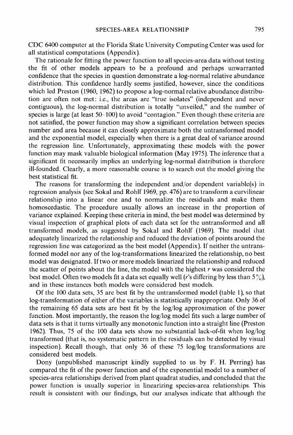
Of the 100 data sets, 35 are best fit by the untransformed model (table 1), so that log-transformation of either of the variables is statistically inappropriate. Only 36 of the remaining 65 data sets are best fit by the log/log approximation of the power function. Most importantly, the reason the log/log model fits such a large number of data sets is that it turns virtually any monotonic function into a straight line (Preston 1962). Thus, 75 of the 100 data sets show no substantial lack-of-fit when log/log transformed (that is, no systematic pattern in the residuals can be detected by visual inspection). Recall though, that only 36 of these 75 log/log transformations are considered best models.

Dony (unpublished manuscript kindly supplied to us by F. H. Perring) has compared the fit of the power function and of the exponential model to a number of species-area relationships derived from plant quadrat studies, and concluded that the power function is usually superior in linearizing species-area relationships. This result is consistent with our findings, but our analyses indicate that although the


TABLE 1

SUMMARY OF THE "BEST MODEL" ANALYSES; (A) FOR ALL STUDIES AND (B) WITH THOSE BEST FIT BY THE UNTRANSFORMED MODEL (35 studies) REMOVED

MODELS

S/A S/LA LS/A LS/LA A

Highest r ............................. .. 50 52 24 53 No "lack-of-fit" .. .......................... 47 38 22 75 Both (Best fit) ................ ........... 35 27 14 43

B Highest . .32 11 45 No "lack-of-fit".... 24 7 44 Both (Best fit) . .19 5 36

NOTE.-Entries indicate the number of times a particular model possessed the highest r, no "lack- of-fit," or both these characteristics. There were studies for which two or more models fit equally well, since we did not discriminate between correlation coefficients that differed by less than 5 %. As a result, the rows do not sum to 100. S/A = untransformed model; S/LA = species/logarea model; LS/A = logspecies/area model; LS/LA = logspecies/logarea model.

power function may often be superior to the exponential model it does not provide a better fit substantially more frequently than does the untransformed model.

We can discern no apparent pattern that seems to predict when the log/log model will be the best fit. As noted previously, studies meeting Preston's two assumptions (i.e., true isolates and large total species number) should be best fit by the log/log model. However, when only such studies are considered, less than half (14 of a total 32) are best fit by the power function exclusively (see fig. 1). From the work of Preston (1960), Williams (1964), and May (1975) we might expect the log/log model to fit studies with relatively large area ranges better, as a consequence of higher total species numbers. However, this pattern is not apparent when relationships among the area ranges of these 32 data sets and their best fit models are examined (fig. 1). Neither number of orders of magnitude of area that a data set covers, nor the particular orders of magnitude that are covered, indicate which model should be the best fit.

The apparent linearity of the relationship between species number and area may be the result of sampling a narrow range of areas. A few researchers (e.g., Archibald 1949; Vestal 1949; Niering 1963; Whitehead and Jones 1969; Abbott 1973; Lassen 1975) have noted that the species-area curves for their data sets possess multiple inflection points when a wide range of area is sampled. This observation is a restatement of the concept of breaks in the species-area relationship noted by Cain (1938). In these instances species-area plots are sigmoidal and are not linearized by the transformations we considered. Thus, in order to depict accurately the distribution of species number with area and select a best model, one must sample a wide range of area (Diamond and Mayr 1976).

If log-normal relative abundance distributions predominate in nature then the power function may have theoretical justification. However, since both the log- normal distribution and the power function are so robust their ability to approxi-


\ __________________ 16 2

) 44 46

17 31 27

0 89 44 44 43

-4 74~~~~~~~~~~~~~~~~~~~~~~~~~~~~~~~~~~~~~~~~~~~~~~~~~~~~~~~~~~~~~~~~~~~4

V \_r_ _ 89 102428

Q)

O ~~ ~ ~~~~32 17 33

37 3

< ~~ ~ ~~~39 43 AL \ ~~44 45

in) ~~ ~ ~~~~~46 50 5 (V 74 75

-0 ~~89 7 0 94 98

C~~~~~~~~~~ 7

55 24

106_107 105_106 104_-105 103_104 102_103 101 _102 100_101 10-1 10? 10-2 lo-,

Orders of Magnitude of Area Covered

FIG. 1.-Area ranges covered by the 32 studies meeting Preston's criteria (i.e., true isolates and large numbers of species). The studies are grouped by their best-fit models in order to show the lack of relationship between area range and best-fit model. Each line represents the area range of a single species-area curve. The numbers placed at the ends of the lines refer to the studies as numbered in the Appendix.

mate the distribution of abundances and species numbers may reflect nothing more than the central limit theorem (May 1975). These properties are a strong practical justification for the use of the power function, yet cloud its biological interpretation.

CAN THE PARAMETERS OF THE POWER FUNCTION BE INTERPRETED

STATISTICALLY AND BIOLOGICALLY?

Prior to 1960, discussion centered on the best-fit model of the species-area relationship and accurate prediction of species number. Many recent analyses, however, have attempted to interpret the slope and intercept parameters of the power function. Gleason (1922, 1925) and Arrhenius (1921, 1923) originally considered the parameters of the species-area relationship to be arbitrary fitted constants. Concomi- tant with the hegemony achieved by Preston's power function model was the development of the idea that the parameters of the power function possessed biological significance. This concept was first manifested by Preston's (1962) prediction of a "canonical" 0.262 value of the slope parameter of the power function caused by the hypothesized log-normal distribution of individuals into species. Sub- sequently, most publications of estimated values of the parameters of the power function have suggested biological interpretations and attempted to compare these parameter values. In disciplines other than ecology the power function has frequently been applied to the description of biological phenomena. It has been used widely in morphological (Huxley 1932; Gould 1966), fisheries (Ricker 1973), physiological (Gunther and Guerra 1955; von Bertalanffy 1957) and other analytical contexts (see


Gould 1966; Zar 1968), in many of which biological interpretations are suggested for its parameters. The parameters of the exponential species-area model, although receiving some attention from plant ecologists, have generally been ignored along with the parameters of the untransformed and logspecies/area models. Before discussing the substance of these interpretations and comparisons, we describe the techniques used to obtain these parameter estimates and detail statistically correct procedures for comparing and drawing inferences from them.

In practice data are seldom fitted to the power function per se, but are usually fitted to its log/log transformation. In both the exponent z is the slope of the line. The power function has an assumed y-intercept (A = 0) of 0, while its log/log transformation has a y-intercept (A = 1) of log k (see eq. [1] and [2]). As pointed out by Zar (1968), fitting data to the log/log transformation yields only approximate estimates of the parameters of the power function, and may in fact produce significantly different estimates of z, especially when r < 1 (which often occurs in species-area analyses). Nevertheless, the log/log transformation is assumed equivalent to, and has been used to estimate k and z values from, the power function in species-area relationships with, we believe, only one exception (Sepkoski and Rex 1974).

The exponential or species/logarea model possesses a slope of z and a y-intercept of log k. The untransformed and the logspecies/area models, which are of the forms

S = zA + k (4) and

log S = zA + k, (5)

respectively, have slopes z and y-intercepts k. Neither the untransformed nor the logspecies/area models are in use in simple species-area analyses (see however, Moore and Hooper 1975; Strong et al. 1977), but have been included in multiple regression analyses of species number (Johnson and Simberloff 1974; Strong et al. 1977). The exponential model, as stated previously, was originally proposed by Gleason (1922) and has commonly been employed in botanical studies.

Estimates of the parameter values (z, k, log k) have always been obtained from model I least-squares regression. In model I regression, only the dependent variable is assumed to be subject to measurement error. However, it is quite common in species-area relationships to encounter a sizable error in the measurement of the independent variable, area. When the assumption of no measurement error in the independent variable is violated, least-squares regression will systematically under- estimate the slope (Ricker 1973). To alleviate this problem two alternatives are available, the "Berksen case" and model II regression. In the Berksen case (Ricker 1973), measurement error is permitted but controlled by the experimenter (e.g., island areas selected a priori; 10 kM2, 100 kmi2, 1,000 km2, etc.). In species-area studies, the measurement error in area is uncontrolled, and therefore model II regression should be used. Ricker (1973), who provides an excellent review of the problem, recommends the reduced-major-axis (geometric mean) regression method, although others (Jolicoeur 1968; Pilbeam and Gould 1974) prefer major-axis regression (the first principal component). We have computed both least-squares and reduced-major-axis parameter estimates for our analyses, although we will discuss only least-squares estimates because similar trends in slopes and intercepts were


obtained using both techniques. Reduced-major-axis parameter values are, however, consistently higher than least-squares values (tables 2 and 3).

Regardless of the particular model, the interpretation and comparison of parameter estimates is constrained by the prerequisites and assumptions of the formal statistical procedures used in their estimation. The slope parameter (z) and intercept parameter (k or log k) may be compared to some hypothesized value (e.g., Preston's canonical 0.262 for z or 1 for log k) through the application of the appropriate t test (Sokal and Rohlf 1969). Comparisons among z values, although slightly more difficult, may also be accomplished by the application of the appropriate t test or by analysis of covariance (Sokal and Rohlf 1969), but additionally require that the range of values of the independent variable (area in this case) overlap considerably between studies (i.e., if islands in archipelago A range in area between, say, 1 and 105 kM2, then the island areas of archipelago B must either be completely included within, or comprise a majority of, this range). The comparison of intercept parameters between regressions is similarly constrained and the appropriate t test is identical to that for the comparison of slopes between regressions, with the values of the intercepts and their standard errors appropriately substituted. However, the slope and intercept of the power function are interdependent parameters, and as a result only intercepts from regressions of equal slopes can be compared (White and Gould 1965). Tests for differences in intercepts are only available for parallel lines, since no sure technique to separate the effects of the correlation between slope and intercept on the intercept from real differences in the intercept is available.

In some models either the slope or the intercept parameters depend upon the measurement units of the independent variable, area. The estimate of the slope is unaffected by the measurement units of area in the power function and exponential models; they need not be in the same units in two regressions for comparison purposes. However, the intercepts, k in the power function and log k in the exponential model, depend upon the units of area measurement. In the untransformed and logspecies/area models, the intercept is independent of and the slope dependent upon the units in which area is measured.

An additional problem in estimating and comparing intercepts arises when small areas have not been included in the regression (Diamond and Mayr 1976). For the untransformed and logspecies/area models this means islands approaching 0 area; and for the power function and exponential models islands at least as small as 1 unit of area. When such points are not included in the regression, estimating and interpreting the intercept values amounts to extrapolating beyond the ends of the regression line, where the confidence intervals flare dramatically (Haas 1975). As pointed out by Sokal and Rohlf (1969, p. 426-427), "... one should be very cautious about extrapolating from a regression equation if one has any doubts about the linearity of the relationship." The inherently asymptotic behavior and possible sigmoidal form of the species-area relationship raise such doubts.

Interpretation of the Slope Parameter

A particularly interesting characteristic common to all models of the species-area relationship is the rate at which species accumulate with increments in area. In linear


TABLE 2

MEANS, STANDARD DEVIATIONS, MINIMUMS, AND MAXIMUMS OF LEAST-SQUARES AND REDUCED-MAJOR-AXIS SLOPE VALUES FOR EACH OF THE FOUR MODELS

SLOPE VALUES

Mean SD Minimum Maximum No.

Untransformed model Least-squares ........ ........... 40.130 281.497 -.000 2,645.093 90 RMA .......................... 62.248 467.443 .000 4,415.848 90

Log/log model Least-squares ........ ........... .310 0.227 -.276 1.132 90 RMA .......................... .468 0.285 .114 1.700 90

Species/logarea model Least-squares ........ ........... 38.831 98.587 -442.640 486.430 90 RMA .......................... 81.014 181.005 2.088 1,361.969 90

Logspecies/area model Least-squares ........ ........... 1.083 4.493 -.000 31.411 90 RMA .......................... 1.715 7.967 0 65.033 90

NOTE.-Ten of the 100 studies are not included in this analysis since the area measurements were in

linear, cubic, or other measurements not readily converted to km2. The studies deleted are listed in the Appendix as numbers 91-100. Values of "-.000" indicate small negative numbers.

TABLE 3

MEANS, STANDARD DEVIATIONS, MINIMUMS, AND MAXIMUMS OF LEAST-SQUARES AND REDUCED-MAJOR-AXIS INTERCEPT VALUES FOR EACH OF THE FOUR MODELS

INTERCEPT VALUES

Mean SD Minimum Maximum No.

Untransformed model Least-squares ......... .......... 69.852 214.990 - 23.672 1,626.268 90 RMA .......................... 50.651 157.737 - 84.548 1,060.492 90

Log/log model Least-squares ........ ........... .704 1.153 -4.402 3.695 90 RMA .......................... .274 1.518 - 8.728 3.652 90

Species/logarea model Least-squares ........ ........... 8.405 446.869 - 733.762 3,887.370 90 RMA .......................... -172.285 655.154 - 5,734.608 375,062 90

Logspecies/area model Least-squares ......... .......... 1.163 .668 -.440 3.142 90

RMA .......................... 1.055 .681 - 1.070 3.121 90

NOTE.-Ten of the 100 studies are not included in this analysis since the area measurements were in linear, cubic, or other measurements not readily converted to km2. The studies deleted are listed in the

Appendix as numbers 91-100.


models this rate of accumulation is represented by a single parameter, the slope of the line, and as a consequence of the assumed linearity of the model is a constant value. Curvilinear models treat the rate of accumulation of species as a constantly changing value (hence the inherent curvilinearity of the model) described by one to a few parameters. Because of the relative ease of manipulation and interpretation, linear models and linear approximations to curvilinear models have naturally been preferred. Of the four linear models we have examined, only the parameters of the log/log approximation to the power function have been the subject of considerable interpretive effort. The following discussion of interpretations of the slope parameter will predominantly concern the log/log model with only passing references to the other models.

The averages and ranges of least-squares and reduced-major-axis estimates of slope values encountered in our set of 100 species-area curves from the four linear models are presented in table 2. In all four models, large positive values indicate high rates of species accumulation with increments in area, whereas small values indicate low species accumulation rates and negative values an absolute impoverishment of large areas relative to small ones. In the log/log model, a slope value of 1.0 indicates that species number and area are "isometric" (sensu Gould 1966). Slope values above 1.0 indicate a relatively greater number of species per unit area in large than in small areas, and slope values between 0.0 and 1.0 indicate a diminishing return in species number per unit area (Abele and Connor 1978).

Preston's canonical 0.262 slope and the regularity of observed z-values. The first statement concerned with the pattern in the value of the slope parameter was Preston's prediction of a canonical 0.262 slope value in the log/log model; many empirically obtained values were consistent with this figure. Although Preston (1962) noted that the logspecies/logarea curve derived from his canonical log-normal relative abundance distribution has a slope of 0.262, errors in sampling and other factors cause variation about this canonical value. Thus, Preston (1962) considered values of about 0.17 to 0.33 to be within the canonical range, while MacArthur and Wilson (1967) accepted values of about 0.20 to 0.35. Preston's "canonical hypothesis" was that the parameter y of the underlying log-normal distribution is 1, which yields his predicted slope value. May (1975), using a set of realistic but noncanonical log-normal relative abundance distributions (y = 0.60-1.70), derived slopes in the range of 0.15 to 0.39. Finally, Schoener's (1976) modification of the equilibrium model leads to slopes between 0 and 0.50. It has become axiomatic that a slope within the circumscribed range noted above (about 0.20 to 0.40) is a singular consequence of deriving a logspecies/logarea relationship from an underlying log- normal relative abundance distribution. However, a few researchers (May 1975, Schoener 1976) have suggested that the result may more likely be a mathematical coincidence. We agree that coincidence is involved, and illustrate here why the slopes of the log/log curves fall regularly between 0.20 and 0.40.

Consider the equation relating the regression coefficient, or slope of the regression line z, to the correlation coefficient r:

z = r(sy/sx), (6)


TABLE 4

CONSTRUCTION OF THE EXPECTED VALUES OF THE REGRESSION COEFFICIENT (Z) WITH THE CONSTRAINTS 0 < r < 1 AND 0 < sls,, < 1 (see eq. [6]).

sy/sx

r .1 .2 .3 .4 .5 .6 .7 .8 .9 1.0

.1 .......... .01 .02 .03 .04 .05 .06 .07 .08 .09 .10

.2 .......... .02 .04 .06 .08 .10 .12 .14 .16 .18 .20

.3 .......... .03 .06 .09 .12 .15 .18 .21 .24 .27 .30

.4 ........... .04 .08 .12 .16 .20 .24 .28 .32 .36 .40

.5 ........... .05 .10 .15 .20 .25 .30 .35 .40 .45 .50

.6 ........... .06 .12 .18 .24 .30 .36 .42 .48 .54 .60

.7 ........... .07 .14 .21 .28 .35 .42 .49 .56 .63 .70

.8 ........... .08 .16 .24 .32 .40 .48 .56 .64 .72 .80

.9 ........... .09 .18 .27 .36 .45 .54 .63 .72 .81 .90 1.0 ........... .10 .20 .30 .40 .50 .60 .70 .80 .90 1.00

where sy and sx are the standard deviations of the dependent and independent variables, respectively (Draper and Smith 1966, p. 35). Allowing that the value of r falls between 0 and 1 (as it must for a positive correlation) and that sy < sx (because of the asymptotic behavior of species number), we construct the relationship shown in table 4 simply by multiplying the marginal values of r and sy /sx to yield slope values (eq. [6]).

Even with these conservative assumptions, 30% of the slopes are expected to fall between 0.20 and 0.40. However, of the 100 species-area curves we examined, 4500 had log/log slope values between 0.20 and 0.40, (see fig. 2). Since the ranges of r and sy/sx of our 100 species-area relationships, and we assume of most analyses, tend to be much smaller, then slope values between 0.20 and 0.40 should be, and are, more frequently observed. The question most germane to this problem is why do r and sy/sx have such narrow ranges?

Values of the correlation coefficient r are usually above 0.50 for logspecies/logarea regressions, most likely because insignificant correlation coefficients are not published, and because both variables are log-transformed. The observed narrow range of sy /sx (usually between 0.20 and 0.60) is a consequence of the asymptotic behavior of species number; once species number becomes asymptotic, area can be increased virtually indefinitely, and concurrently sy/sx and the slope will decline. In other words, since species-area curves are characterized by inherently larger ranges of areas than species numbers, the numerator of the term sy /sx will always be smaller (usually much smaller) than the denominator. Hence, the small fractional values of sy/sx multiplied by r (see eq. [6]) produce lower slopes the larger the area range.

In essence, our contention is that the narrow range of observed slope values (0.20-0.40) is more parsimoniously explained to result from the characteristics of the regression system, and not from underlying log-normal relative-abundance distributions. One might argue that the observation of 45/100 slope values between 0.20 and 0.40 merely confirms May's (1975) observation on the robust nature of the noncanonical log-normal relative abundance distribution and does not really demonstrate


30

expected- D FIG. 2.Cmprso f xece adobserved- lu

0.

o 0.

0 0 5

0.0 0.1 0.2 0.3 0.4 0.5 0.6 0.7 0.8 0.9 1.0

Slope Classes (z FIG. 2.-Comparison of expected and observed log/log slope values. Expected proportions of

slope values for particular classes were generated by summing the entries in table 4 and dividing by 100 for each class. Observed proportions were similarly derived from the data in the Appendix. Slope values exceeding 1 or less than 0 (2 values each) were tabulated within the highest and lowest slope-value classes, respectively.

any mathematical coincidence. We counter this by noting that of the 36 data sets best fit by the log/log model (see table 1), only 15 have slopes between 0.20 and 0.40. This observation means that a slope between 0.20 and 0.40 is often obtained even when fitting the log/log model to data probably lacking an underlying log-normal relative abundance distribution.

Furthermore, in a completely unrelated discipline, slopes between 0.20 and 0.40 also show up consistently. In brain weight-to-body weight allometric regressions, intraspecific plots uniformly show a slope of 0.20 and 0.40 (Pilbeam and Gould 1974 and included references). This functional relationship is maintained by organisms displaying similar body plans over a wide size range. Interspecific plots of animals having an allometric relationship of brain weight to body weight display a higher slope (nearly always 0.66), and those with increased cephalization, an even higher one (greater than 1). Here again, in the intraspecific plots the range of the dependent variable is always much less than that of the independent variable (syl/s. exhibits small fractional values), r's are very high (usually greater than 0.90), and the slope almost always falls in the interval 0.20 to 0.40. In interspecific plots the range of the dependent variable is automatically increased (because of greater variability in size between adults of different species than among adults of the same species), therefore syl/s. and the slope increase also.

The regular occurrence of slope values between 0.20 and 0.40 thus seems to be an expected characteristic of any regression system with a high r value and a small range in the dependent variable relative to that in the independent variable. Although species-area curves derived from an underlying log-normal relative abundance distribution also display a similar narrow range of values, slope values in this range can be expected regardless of the underlying relative-abundance distribution. When interpreting slope values we suggest, to borrow a phrase from Gould (1971), that slopes in the 0.20 to 0.40 range (approximately) be considered as a "criterion of subtraction," or as the null hypothesized range of slope values, perhaps indicating correlation between species number and area without a functional relationship. It may be that only slope values deviating from this range possess biological significance.


0 U5

non-isolates noe isolates far Isolates non-isolates near isolates far isolates MacArthlr & Wilson's (1967) View Schoenerd s (1976) &

Diamond & Mayr's (1976) View

FIG. 3.-Diagrammatic representation of MacArthur and Wilson's (1967), Schoener's (1976), and Diamond and Mayr's (1976) hypotheses concerning the relationship of the slope value of the power function to isolation.

Island versus continental differences in the slope parameter. We have seen that, based on the assumption of an underlying log-normal relative-abundance distribution, Preston (1960, 1962) predicted that the slope value of the log/log model for true isolates should be in the range 0.20-0.40. Deviations in observed slope values from the theoretical value were attributed to increases in habitat diversity (higher values) or to sampling nonisolated areas (lower values). Preston (1960) envisioned sampling from nonisolated areas as sampling from a truncated log-normal relative abundance distribution in which the ratio of species to individuals is much higher than in the complete log-normal distribution characteristic of an isolate. As a result, small areas would be overrich in species and the slope of the species-area curve would be depressed below the canonical value. Preston (1960) made his original observation of these low slope values in species-area curves for the Nearctic (z = 0.12) and Neotro- pical (z = 0.16) avifaunas. MacArthur and Wilson (1967) restated Preston's (1960) idea, proposing that slope values derived from nonisolated areas, either within islands or within continents, should fall in the range 0.12-0.19. They argue that since many transients will be encountered in the nonisolated areas, independent of area, species numbers in small areas will be inflated, depressing the slope of the logspecies/logarea curve (see fig. 3). Although not suggested by MacArthur and Wilson (1967), it is also wise to confine predictions to comparisons within taxa or other groupings of species with similar dispersal abilities.

Preston (1960) and MacArthur and Wilson's (1967) prediction of lower continental than island slope values can be interpreted literally or liberally. Their hypothesis could be considered falsified if the predicted pattern of slope values, in the specified ranges (0.12-0.19 for continents and 0.20-0.40 for islands) does not obtain. Alterna- tively, we could consider their hypothesis at least qualitatively supported if the predicted differences in slopes occur even though they do not segregate into the specified ranges.

Simberloff's (1976a) experimental work has shown that for nonisolated areas within islands species numbers are in fact inflated for small areas, suggesting that the transient hypothesis is sound. However, he made no attempt to relate his results to the slope value of the logspecies/logarea curve, since his sample size was small and the use of serially self-contained sample areas violates the assumption in regression


that each measurement of the independent variable be derived independently. In addition, Goodall (1952), Greig-Smith (1964), and Kobayashi (1974, 1976) believe that slopes derived by combining random samples will be higher than those derived from the continuous expansion of a single sample, an effect independent of the transient hypothesis.

Adequate data to examine the effect of the transient hypothesis on the slope of the species-area curve are unavailable, but Johnson et al.'s (1968) analysis of the floras of the California Channel Islands and mainland southern California bears on this problem. Johnson et al. (1968) report a slope value for the Channel Islands of 0.472 and a slope value of 0.158 for mainland areas. This result appears to fit Preston's and MacArthur and Wilson's prediction at least qualitatively; however, the area ranges of the island (0.02-134 mile2) and mainland (5.9-24,000 mile2) regressions barely overlap, so the slopes cannot be compared properly. When we compare slope values generated from Johnson et al.'s (1968) data, but with similar area ranges (i.e., deleting islands with areas less than 1 mile2 and mainland sites with areas greater than 529 mile2) the island (0.06) and mainland (0.27) slope values differ as per MacArthur and Wilson's and Preston's prediction. However, these values still do not segregate into the predicted ranges. Preston's (1960) original observations of low slope values in the nonisolated Nearctic and Neotropical avifaunas are subject to the same criticism. The area ranges covered by these continental studies are tremendously greater than those of any island archipelago. The behavior of these slope values could result from depression of species numbers in large areas, because of the asymptotic nature of species numbers, rather than the inflation of species numbers caused by more transients in small areas. Brown's (1971) study of the montane mammals of the great basin also appears to support the transient hypothesis and its effect on the slope of the logspecies/logarea curve. However, Brown's mainland (nonisolated) slope value was based on four sample areas, none of which were within the range of area covered by the comparable small isolates, exactly the range critical to a test of the transient hypothesis.

Low slope values have also been obtained for truly insular situations (isolates). Case (1975) reported a slope of 0.166 for the lizards of the California Channel Islands, Baroni-Urbani (1971) a slope of 0.188 for the ants of the Tuscan archipelago, and Harris (1973) a slope of 0.157 for the birds of the Galapagos. This evidence falsifies MacArthur and Wilson's (1967) prediction of isolate slopes falling exclusively in the 0.20-0.40 range (or at least not below 0.20), but remains open to the interpretation that were the slopes for those taxa known for adjacent nonisolated mainland areas, they would be comensurately lower.

The evidence indicates that the postulated effect of transients on slope values from nonisolated areas remains testable when interpreted broadly. Although slope values from some isolated areas fall within the predicted range for nonisolated areas, actual slopes from nonisolated areas could be lower yet. The relatively low correlations (r < .9) observed between species numbers and area in most instances, and their considerable range, could possibly mask this pattern if it exists.

Isolation and the slope parameter.-It has long been known that geographically isolated archipelagos possess depauperate biotas. Hamilton et al. (1963) and later others (Simpson 1974; Power 1972; Johnson and Simberloff 1974; Johnson et al.


1968, etc.) have demonstrated that isolation explains a significant amount of the variation in species number. Utilizing stepwise multiple regression analyses, each of these workers concluded that isolation accounts for the reduced numbers of species after the effect of area has been factored out.

In view of this pattern, MacArthur and Wilson (1967) proposed a parallel phenomenon for the slope of the species-area relationship. Their prediction, based on equilibrium theory, was that the slope of the species-area curve would be higher for distant or isolated archipelagos (fig. 3). This explanation is an extension of the transient hypothesis offered for island versus continent differences in the slope parameter (Preston 1960; MacArthur and Wilson 1967). The idea that isolated archipelagos have fewer transients caused by lower immigration rates has been challenged by Abbott and Grant (1976).

MacArthur and Wilson (1963) were able to muster little evidence to support their prediction; and subsequently Hamilton and Armstrong (1965) observed a decreased slope with isolation, exactly opposite MacArthur and Wilson's prediction (fig. 3). Schoener (1976) provides the best and most complete analysis of this question to date. He plotted the slope values obtained for land and freshwater birds from 23 archipelagos versus isolation and confirmed the result of Hamilton and Armstrong, that the slope decreases with isolation. We performed analyses similar to Schoener's and show an identical trend. For the total birds subset (17 studies, see section on the Latitudinal dependence of the species-area relationship for a detailed explanation concerning how this subset was constructed) Spearman correlation coefficients were computed between the slope parameter and isolation distance. The results show that the log/log slope is significantly negatively correlated with isolation (r = -.6872, P = .004).

Schoener's explanation for this relationship is that the slope of the species-area curve is dependent upon the size of the source pool of species, which in the case of distant archipelagos will be small, therefore lowering the slope. However, Schoener's explanation may not apply to all taxa since distant archipelagos may have smaller source pools without having lower slopes if the intercept also changes with isolation (fig. 4). We can see from this problem that although trends in the slope or intercept with isolation may be observed, we have no means of predicting their form. Even if the pattern observed by Schoener (1976) and Hamilton and Armstrong (1965) was determined to be ubiquitous, it reveals little more than has long been established: Distant archipelagos have depauperate biotas.

Equilibrium theory explanations of variation in slope. Numerous authors have attempted to explain variation in the log/log slope value in terms of the "equilibrium theory" proposed by Preston (1960) and MacArthur and Wilson (1963, 1967). Equilibrium theory considers species number to be the result of a dynamic balance between immigration and extinction of species. Species number may be affected by either process individually (varying immigration or extinction rates) or both simultaneously. An interrelationship between immigration and extinction rates and the parameters of the species-area curve, although never fully explored, has been assumed to exist (Ricklefs and Cox 1972). As previously stated, MacArthur and Wilson (1967) first predicted that high immigration rates would decrease the slope of the species-area relationship. Subsequently Brown (1971), Terborgh (1973), and Strong and Levin (1975) have interpreted empirically derived estimates of the slope


species pool for near isolates

..,-curv for near isolates

W species pool for S ' for isolates (I)

o3 L curve for for isolates

LOG AREA

FIG. 4.-Illustration of how the slope of the species-area curve is potentially independent of the size of the source pool of species. In this example the slopes of the hypothetical species- area curves are equal even though the source pool of the distant archipelago is smaller than that of the near archipelago, because the y-intercept value of the curve for the distant archipelago is changed.

(z) in such a manner. However, Johnson and Simberloff (1974) point out that even within the equilibrium theory context low z values are not uniquely explained by high immigration rates, but likewise by low extinction rates or by a combination of high immigration and low extinction rates. Thus, three alternative hypotheses can be generated from a single theoretical framework (equilibrium theory), whose uncritical acceptance has been criticized by Lynch and Johnson (1974) and Simberloff (1976b).

An additional problem is that of establishing ultimate causality. Strong and Levin (1975), for example, postulate that the relatively low z value for the parasitic fungi of British trees compared to that of the phytophagous insects of British trees is due to high immigration rates for fungi. Their logic derives from the anemochorous dispersal of fungal spores. Even given this dispersal characteristic, the ultimate cause of the low z value for fungi may be due to a depauperate species pool, inasmuch as the high dispersibility of fungal spores would inhibit diversification through allopa- tric speciation. This latter alternative, that of an evolutionary difference in insect and fungal diversification caused by dispersibility, and Strong and Levin's equilibrium theory model must be viewed as competing hypotheses.

As discussed by Simberloff (1976b), equilibrium theory, like the log/log model of the species-area relationship, has been elevated to the status of a paradigm. Moreover, the ascendency of equilibrium theory as the major underlying theoretical framework in biogeography and population ecology has motivated many workers to interpret their results within the framework and to consider successful interpretation prima facie evidence of the veracity of the interpretation. Equilibrium theory and ideas interpreted within its framework must be restated as testable hypotheses, not accepted as proven.


Interpretation of the Intercept Parameter

The intercept parameter (y-intercept value) has been virtually ignored as a quantity deserving biological or statistical explanation, or as a basis for biological inferences. MacArthur and Wilson (1967) consider it solely as a fitted constant relating to local environmental conditions. Unlike the slope parameter, no regularly recurring values have been reported and no "canonical" value hypothesized. MacAr- thur's (1965, 1969) treatment of the latitudinal relationship of the species-area effect and Johnson and Raven's (1970) view that the intercept will decrease with increasing latitude are the only attempts to explain geographic patterns (in this case purely hypothetical) in the intercept parameter.

The averages and ranges of least-squares and reduced-major-axis estimates of intercept values encountered in our set of 100 species-area curves from the four linear models are presented in table 3. As mentioned previously, the untransformed and logspecies-area intercept parameters are not dependent on the measurement units of area, whereas the log/log and species/logarea parameters are. Biologically realistic values of the intercept parameter in the untransformed and logspecies/area models are values of 0.0 and below; positive values of the intercept parameter in these models would indicate the unlikely situation that in a sample of no area there exists some number of species. In practice, parameter values greater than zero are commonly found (see Appendix), and as a result are uninterpretable in these instances. Biologically realistic values of the intercept parameter in the log/log and species/logarea models contain a large range of real numbers. Positive values indicate that some number of species (if 1.0 or greater) will be found or that a probability of finding species (if between 0.0 and 1.0) exists when a sample of one unit of area is examined. Negative or zero values of the intercept parameter in these models indicate that no species will be found in a sample of one unit of area.

Heatwole (1975) suggests that, because of the uninterpretable values often obtained for the y-axis or species-intercept, we abandon attempts to attach biological significance to it and use instead the x-axis or area-intercept. Heatwole considers the x-intercept to be an indication of the "minimal area" necessary to support a breeding population of the particular taxon being studied. Hopkins (1957) previously discussed the term "minimal area" in plant community analyses; however, his usage is completely different from Heatwole's. Currently, Heatwole's suggestion remains an unexplored possibility.

The intercept parameter may, in fact, be affected by local environmental conditions or other factors (MacArthur and Wilson 1967), but concrete demonstration of these relationships and an assessment of their proportional contribution to its variation would be enormously difficult, since the proper analysis must follow the procedures described above. Assembling a large enough subset of intercept values from species-area curves with homogenous slopes that simultaneously vary with respect to the environmental conditions under study would probably be impossible. The same factors that may potentially cause variation in the intercept are likely to have similar effects on the slope parameter, thereby precluding the examination of their relationship to the intercept parameter. Because of these analytical problems, and also the lack of any a priori theoretical framework for its biological significance, the intercept parameter must be considered simply a fitted constant.


The Partitioning of Alpha and Beta Diversities into the Slope and Intercept Parameters

Whittaker (1960) first introduced the concept of alpha, or within habitat, and beta, or between habitat, diversity in 1960 as an attempt to partition diversity into independent components. MacArthur (1965) attempted, in part, to unify conceptual treatments of diversity using the species-area curve as an analytical tool by suggesting that the intercept parameter was a measure of alpha diversity and the slope parameter a measure of beta diversity.

Inasmuch as the concepts of alpha and beta diversity treated these components as independent, the attempt to establish their proportionality to the parameters of the log/log species-area model was doomed from the start. Since the slope and intercept of the power-function are algebraically interdependent parameters (White and Gould 1965, Gould 1966, 1971), when slope changes occur (caused, according to MacArthur, by adding or deleting habitats) it is impossible to compare the newly generated intercept to the pre-slope-change intercept since no statistical procedure exists to separate differences between intercepts caused either by the slope or by real changes in the intercept. Therefore, in MacArthur's system a change in slope precludes identifying a change in intercept.

Beyond the critique on statistical grounds, some empirical observations on the slope parameter are also pertinent. Several workers have prepared species-area curves for "single-species habitat islands"; Strong (1974b) and Strong et al. (1977) for phytophagous insects on host plant islands and Abele (1976) and Abele and Patton (1976) for decapod crustaceans on "coral head islands." Southwood (1960), Janzen (1968), and Strong (1974a) all contend that many phytophagous insects view single plant species as a habitat. Abele and Patton (1976) give convincing evidence that single-species coral heads are a single habitat by demonstrating that all decapod associates are found on a complete size range of coral heads. If the slope from the log/log species-area model is a measure of between-habitat diversity, as suggested by MacArthur, we would expect slope values of zero for these within-habitat studies. Instead, we observe values of z ranging from 0.327 to 0.370 (all significantly different from zero, P < .05). In essence, as we add area of the same type of habitat we add species and therefore generate a "within-habitat slope" (which is consistent with the area-per se hypothesis). Although it is possible that slope values would be higher if habitats were added, it is evident that between-habitat diversity does not account completely for observed slope values.

As shown above, even for simple systems some component of the slope is probably due to within-habitat diversity. For more interesting cases, such as archipelagos of true islands, we have no way of enumerating the numbers of habitats or their respective areas in order to attribute differences in slopes or intercepts to changes in alpha or beta diversities. We therefore consider it logically and practically impossible to apportion alpha and beta diversities to the intercept and slope parameters.

The Latitudinal Dependence of the Species-Area Relationship

MacArthur (1965, 1969) predicted that concomitant with latitudinal gradients in species number (either total or mean species number for equal sized areas) one


should observe latitudinal gradients in either or both of the parameters (slope and intercept) of the power function. This prediction, in tandem with his attempt to apportion within-habitat and between-habitat diversity to the intercept and slope parameters, led him to conclude that an investigation of the latitudinal dependence of the slope and intercept of the species-area relationship would enable one to discriminate between three alternative explanations for the existence of latitudinal diversity gradients. MacArthur reasoned that (1) if only the intercept was inversely correlated with latitude then latitudinal diversity gradients could be attributed to increased within-habitat diversity in the tropics, (2) if only the slope was inversely correlated with latitude then latitudinal diversity gradients were due to increased between-habitat diversity in the tropics, and (3) if both the intercept and slope were inversely correlated with latitude then latitudinal diversity gradients were due to increases in both within-and between-habitat in the tropics. However, as suggested above, within- and between-habitat diversity cannot be apportioned to the intercept and slope parameters for both statistical and biological reasons. A further problem stems from the lack of any technique for comparing intercepts between studies with unequal slopes. Thus, if a relationship exists between the slope and latitude, it precludes detecting any relationship between the intercept and latitude. As a result, MacArthur's third alternative, given contemporary analytical methods in parametric regression, could not be demonstrated even if it were the correct alternative.

Although the theoretical framework suggested by MacArthur for the interpretation of trends in the relationship between the slope or intercept of the log/log species-area model and latitude seems incorrect, the original prediction that a trend will exist is still worthy of examination. The basic question is: Given that we observe latitudinal gradients in total species number and mean number of species per unit area, should we expect to observe similar trends in the parameters (slope and intercept) of an empirically fitted model of the entire distribution of species number with area? To answer this question we again examine our set of 100 species-area curves, contrasting MacArthur's predictions as a set of alternative hypotheses against the null hypothesis that no trends exist. We will consider the relationship between the slope parameter and latitude, the intercept parameter and latitude, and, although not a part of MacArthur's prediction, the linear correlation coefficient and latitude.

Slope and latitude.-In order to examine the relationship between the slope parameter and latitude, we obtained subsets of studies within which valid comparisons of slopes could be made. To compare slopes from two species-area curves, each study must span similar area ranges or at least overlap considerably. To this constraint we added the requirement that comparisons be made only within taxonomic levels (orders, families, etc.). Since lower taxonomic levels are inherently less diverse than higher ones, for the same area range their slopes will automatically be lowered and could therefore generate spurious correlations or mask real correlations between the slope parameter and latitude. For example, slopes of species-area curves for vascular plants should not be compared to slopes of species-area curves for grasses only. The same problems could occur if studies of mixed taxonomic groupings (e.g., mammals, vascular plants, insects, and fish) were compared, since each taxa does not represent a constant proportion of the biota.

Given these two constraints, we determined that out of 100 species-area relation-


TABLE 5

RELATIONSHIP BETWEEN THE SLOPE PARAMETER AND LATITUDE

VALUES OF r

Total Land Land and MODEL Fish Insects Birds Birds FW Birdst

Untransformed ......... - 1.000* -.4000 -.2108 .5000 -.6000 log/log ................ - .4000 0 - .0833 - .4000 .4000 Species/logarea ......... -.4000 0 -.4926* - 1.000* 0 logspecies/area ......... -.8000 -.4000 -.1386 -.5000 0

* Spearman's correlation coefficients between slope values and latitude means for each study in a subgroup (significant correlations, P < .05, are indicated by an asterisk; for a listing of studies comprising each subgroup see Appendix.

t FW = freshwater.

TABLE 6

CORRELATION (Spearman's) OF MEAN AND MAXIMUM SPECIES NUMBER WITH LATITUDE FOR TAXONOMIC SUBGROUPS OF SIMILAR AREA RANGE

Subgroup Mean No. logmean No. of Max No. of logmax No. of

Total birds (17) ......... ...... -.6005* -.5956* -.5294* -.5294* Land birds (5) ......... ....... - 1.000* -.9000* -.9000* -.9000* Land & freshwater birds (4) .... 0 0 0 0 Insects ...................... .8000 .8000 .2000 .2000 Fish (4) ...................... -.6377 -.5218 -.4478 -.4478

NOTE.-The procedures used in constructing the subgroups are described in the text. For a listing of the studies included within each subgroup see Appendix.

* P < .05.

ships including numerous taxa, only five subsets fulfilling these requirements could be constructed; total birds (17 studies), land birds (5 studies), land and freshwater birds (4 studies), fish (4 studies), and insects (5 studies). This paucity of comparable studies illustrates the need for the continued examination and enumeration of species-area relationships.

Nonparametric correlation coefficients (Spearman's) were computed between the slope parameter and latitude for each of the four models of the species-area relationship being considered. The results of these analyses are presented in table 5. Both the mean and maximum number of species in each species-area relationship are significantly negatively correlated with latitude in only two of these subgroups, total birds and land birds (table 6). For land and freshwater birds, insects, and fish neither mean nor maximum number of species is correlated with latitude; in other words, no latitudinal gradient in species diversity is demonstrated by these three groups. This is not to say that in actuality land and freshwater birds, insects, and fish exhibit no latitudinal diversity gradient, only that for these particular species-area curves they do not. Since these three subgroups display no latitudinal diversity gradient, it is unlikely, although possible, that pattern in their slope values could be due to latitude. Thus, we attribute little significance to the correlation between the least-squares


estimate of the slope parameter in the linear model and latitude for the fish subgroup (table 6).

Interestingly enough, for the two groups that display latitudinal gradients in mean and maximum species number, significant correlations between the slope parameter and latitude were not demonstrated for the log/log model but were evident for the exponential (species/logarea) model (table 6). When the species-area curves comprising these two groups are examined, either the species/logarea or the log/log are the best-fit models, indicating that the lack of relationship between the slope of the log/log model and latitude cannot be attributed to these subsets' being anoma- lous groupings, which are relatively poorly fit by the log/log model. For those subsets demonstrating latitudinal gradients in mean and maximum species number, only the slope in the exponential (species/logarea) model was significantly correlated with latitude.

Intercept and latitude.-Since intercepts can only be compared among groups of species-area curves with homogeneous slopes, we first constructed subsets by comparing slopes for all possible pairs of species-area curves for each of the four models in both the total birds and land birds subgroups. For the total birds subgroup this amounted to 136 t values per model and for the land birds subgroup 10 t values for each model.

In each subset of values, no slope differed significantly (P < .05) from any other member of the subset, and no other studies meeting these criteria could be added to the subset. For the 17 total bird studies, one subset of six studies in the untransformed model, three subsets of six in the log/log model, two subsets of five in the species/logarea model, and two subsets of six in the logspecies/area model could be constructed. For those models with multiple subsets, the subsets differed in composition from between one and four studies, but never were completely different. No subset of homogeneous slope values common to each of the four models could be constructed. For the five studies in the land birds subgroup, all slopes were significantly different in the untransformed model, one subset of three studies could be constructed in the log/log model, and one subset each of two studies could be constructed in the species/logarea and logspecies/area models. These subsets of the land birds grouping were considered too small for further analysis.

The relationship between intercept and latitude for the total-birds grouping of homogeneous slopes was investigated using Spearman's correlation coefficient. The results of these analyses are presented in table 7. No relationship between intercept and latitude was identified for either the untransformed, log/log, or species/logarea models. For the species/logarea model, where a relationship between slope and latitude had previously been identified, this analysis was actually superfluous since the existence of a slope trend precludes identifying an intercept trend. The results obtained for the logspecies/area model are equivocal. A significant relationship was identified in only one of the two subsets. Again, more and larger subgroups are needed for a complete analysis.

The linear correlation coefficient, r, and latitude.-Several workers (Preston 1962; Schoener 1976; Dony unpublished manuscript) have indicated that there may be an effect of geographic location on the fit of different models of the species-area relationship. To test this proposition we plotted the correlation coefficient derived


TABLE 7

RELATIONSHIP BETWEEN THE INTERCEPT PARAMETER AND LATITUDE FOR HOMOGENOUS

SUBSETS OF SLOPE VALUES IN THE TOTAL BIRDS SUBGROUP

Subgroup r P No. Source Studies

Untransformed ......... ........... - .2571 .312 6 (3,14,21, 39,64,74) log/log ............................ .0286 .479 6 (14, 15, 59, 74, 81, 89)

-.1429 .394 6 (14, 27, 59, 75, 78, 79) -.1429 .394 6 (14,27, 59, 75, 78, 81)

Species/logarea ......... ........... -.6000 .143 5 (15, 21, 59, 60, 89) -.5000 .196 5 (15, 21, 59, 60, 79)

logspecies/area ..................... - .6000 .105 6 (3, 14, 15, 21, 24, 64) -.7714 .037 6 (14,24, 39, 60, 81, 89)

NOTE.-r = Spearman's correlation coefficient and P = level of significance. Subset composition indicated in parentheses refers to studies numbered in Appendix.

L* * * .0

_ 6 *..* **2

0

-5 4 * .

E 0-.2

-4

-.6

I I0 20 30 40 50 60 70 80

Latitude Midpoint

FIG. 5.-Relationship between the linear correlation coefficient of the log/log species-area model and the latitudinal midpoint of each study (r = - .3183, P < .001, N = 100). The relationship remains significant even when negative correlation values are removed.

from the log/log model of our 100 data sets versus latitude. Figure 5 shows that these correlation coefficients are negatively correlated with latitude (r = -.3183, P < .001); that is, log-area explains more of the variance in log-species at low latitudes that it does at high latitudes. The linear correlation coefficient is also significantly negatively correlated with latitude in each of the other three models. It might be suspected that this correlation is spurious, derived from a possible correlation between latitude and the number of data points contained in each study. However, the number of data points in a study is not correlated with latitude (r = .0459, P = .325).

Although the correlation between r and latitude is highly significant, 92% of the variance in r remains unexplained. This is partially due to the heterogeneity of the set of species-area relationships utilized. For example, habitat islands (eight studies) show no relationship between r and latitude, whereas for distant archipelagos (35


studies) latitude explains 49% of the variance in r. Longitudinal variance in species number also contributes to the large residual variance; for instance, studies performed in the British Isles and the Mediterranean region tend to have r's that are higher than those from other regions at the same latitude.

Biologically, the lower correlation between species number and area at high latitudes may be the result of the relatively small source pool of species (as evidenced by latitudinal gradients in species number) and to each species' having on the average a relatively wider distribution than low latitude species (McCoy and Connor, in prep.). Hence, given the few species available to colonize a particular area and their wide distribution, species number rapidly becomes asymptotic for small areas and fails to increase when large areas are examined. Further, stochastic fluctuations in climate serve to maintain disequilibria in species numbers (Abbot and Grant 1976), resulting in a poor relationship between species number and area. Our analyses have revealed that there is no latitudinal dependence of the parameters of the species-area relationship, contrary to MacArthur's prediction. We do, however, confirm his intuition that there is a latitudinal dependence of the species-area relationship, but that it is manifested by the degree of correlation between species number and area, not the slope and intercept parameters.

SUMMARY AND CONCLUSIONS

We have discussed three basic questions concerning the species-area relationship. We now briefly summarize our conclusions, and discuss their ramifications for the future use of the species-area relationship, both its methods and interpretation.

Is there a unique theoretical basisfor the species-area relationship? Our discussion of the theoretical basis of the species-area relationship was basically inconclusive. The two most frequently proposed hypotheses, habitat diversity and area per se are both possibly correct, yet the result of either mechanism is neither qualitatively nor quantitatively different. One virtually always observes a positive correlation between species number and area, regardless of the mechanism. On the other hand, this result can also be explained as a consequence of isolates passively obtaining samples from some species pool, large isolates receiving effectively larger samples and ultimately containing more species than small isolates. It seems plausible that the habitat- diversity hypothesis could be tested by looking at equal sized areas with various numbers of habitats, assuming that habitats could be defined objectively. The area-per se hypothesis requires that one actually demonstrate decreased extinction rates for larger islands (heretofore taken to be a logical assumption), and the sampling hypothesis requires that we demonstrate a direct proportionality between immigration rates and area. There may be at least a grain of truth in each of these mechanisms. Each of these three, and possibly others, may play a role in producing the observed positive correlation between species number and area.

Is there a best-fit model of the species-area relationship? Our analyses of 100 species-area curves indicates that there is no single best-fit model. The best-fit model for a particular species-area curve can only be determined empirically. Of the four linear models we examined, the power function and the untransformed models provide good fits most frequently. Curvilinear models were not examined, even


though when a wide range of areas is sampled the species-area relationship can become sigmoidal. Comparing species-area curves from curvilinear models is inherently more complicated, and it is uncertain that any additional benefit would be derived. We suggest continued use of the power function and other linear models because of the relative ease which they can be compared, and their past and present wide usage.

Can the parameters of a particular model, specifically the power function, be interpreted?-In general, we have found that published predictions and interpretations concerning both the slope and intercept parameters are not supported by the available evidence. Many other predictions and interpretations are either logically untestable or require additional data for an adequate test. Because of these results, we are skeptical that any biological significance can be attached to these parameters and recommend that they be viewed simply as fitted constants devoid of specific biological meanings.

Species-area relationships: methods. A discussion of the methods used in obtaining parameter estimates and comparing parameter values was presented. The use of either model I or model II regression in biology as a whole has usually been a matter of taste left to the discretion of each worker. However, in species-area analyses the degree of error in the independent variable, area, is great enough to warrant considering application of model II regression methods uniformly. The results of comparisons involving least-squares parameter estimates remain unchanged when using model II estimates. In this respect one has some leeway in choosing model I or model II regression, since model II yields more accurate estimates of the parameters, whereas the results of comparing parameter values are the same regardless of whether model I or model II estimates are employed. Obviously one should use model II when attempting to obtain accurate estimates of the parameters, and either model when comparing parameter values.

Perhaps a more fundamental question is whether regression or correlation should be used in species-area analyses. The particular problem under investigation dictates which method is appropriate. Correlation only allows the assessment of the degree of relationship between species number and area, and regression yields parameter values permitting comparisons of the bivariate distribution of species number with area. If one is interested only in the degree of relatedness between species number and area, correlation is the appropriate method. If one wishes to compare two or more bivariate distributions, then regression is the proper technique.

We recommend that each of these methods be used exclusively for the purposes described above. This is actually no more than recommending that biologists use statistics correctly. We especially encourage the publication of nonsignificant correlation coefficients between species number and area, values that now are probably either eliminated by the review process, by an author's disbelief in his own results, or the thought that they are uninteresting. Such examples are as informative about species-area relationships as are significant positive correlations, if not more so.

Species-area relationships: interpretations.-The interpretation of species-area relationships can be based on three criteria, (1) which model is the best fit, (2) the strength of correlation between species-number and area, and (3) how the parameter values compare to other published values.


Although Williams (1964), Preston (1960), and May (1975) have demonstrated that the log-series and log-normal relative abundance distributions are best fit by the exponential and power functions, respectively, the converse is not true. A species- area relationship best fit by an exponential or power function does not indicate an underlying log-series or log-normal relative abundance distribution. Relative abundance distributions can only be determined empirically; although one can predict, as May (1975) has done, that as a consequence of the statistics of large numbers relative abundance distributions are most likely to be log-normal for large species numbers. It may be premature to conclude that demonstrating that a particular model is the best-fit model is uninteresting, but as yet no significance can be attached to any particular model.

The degree of correlation or relatedness between species number and area could potentially be affected by numerous factors. The observation of an inverse relationship between the linear correlation coefficient and latitude may be due to high latitude species' possessing greater geographical ranges; hence few new species are encountered when one examines large versus small areas. No other pattern in the degree of correlation between species number and area has yet been identified. However, only a limited set of coefficients has been published (only significant correlations). The possibility exists that some pattern has been obscured by this practice.

The species-area relationship has unfortunately been used as a justification for conservation practices in which large areas are preserved in preference to small areas, since large areas are considered to contain more species (Terborgh 1974, 1975; Diamond 1975; Wilson and Willis 1975). Although we agree in principle with the preservation of large areas, the species-area relationship does not provide an unambiguous justification. As discussed by Preston (1962), Simberloff (1972), Sim- berloff and Abele (1976), and Abele and Connor (1978), it is both conceptually and actually possible that a group of small preserves contain more species than a single large preserve of equal total area. The dependence of the linear correlation coefficient of species-area curves on latitude also clouds the broad application of recommenda- tions based on the species-area relationship without reference to geographic location. We agree with Simberloff and Abele (1976) that conservation areas should be designed with specific goals in mind, providing the particular habitat requirements for the species to be preserved.

Ultimately, species-area curves will be most useful in comparing diversities between geographical regions, habitats, or taxa over a range of sample sizes, or between different sized samples. Classical diversity measures compare diversities based on a single sample size, whereas species-area curves permit the comparison of the entire distribution of species number with area. Species-area curves can also be used to "factor out" the effect of area on diversity, so that the effects of other variables on species numbers can be determined. Strong (1974a, 1974b) has done this with phytophagous insect diversities in order to examine the effects of time, and Abele (1976) has done this to examine the effects of environmental stability on coral- inhabiting decapod crustaceans. Simberloff (1974), Raup (1976), and Sepkoski (1976) have employed species-area curves to explain the Permo-Triassic extinctions and Phanerozoic diversity trends in shallow-water marine invertebrates, although Raup


views the effect of area (volume of sedimentary rocks) purely as a sampling phenomenon. It is through these comparisons of species-area curves, and only indirectly so, that the parameters of the power function or any other model have biological significance. In the absence of a priori theoretical bases for predictions concerning parameter values, such values must be considered simple fitted constants devoid of biological meaning.

ACKNOWLEDGMENTS

This manuscript benefitted greatly from the careful reading and critical comments of K. L. Heck, D. R. Strong, D. Simberloff, L. G. Abele, and G. Morrison, as well as the consultation of D. Meeter. We thank R. Ricklefs, F. H. Perring, J. Rey, and L. G. Abele for providing unpublished data for our analysis, P. Liepshutz, T. Berman, J. White, and L. Maddox for typing another tedious manuscript, Arlee Montalvo for preparing the figures, and Mike Auerbach for photographic assistance. This research was supported in part by NSF grant DEB 76-07330 to Daniel Simberloff and NSF grant DEB 76-24415 to Donald R. Strong.

APPENDIX

The following table is a list of each of the 100 species-area curves used in our analyses. We have included the source of each data set, the number of localities used to compute each curve, correlation and regression coefficients from all four models discussed in text, and other data pertinent to particular analyses or to the construction of subgroups for analysis. Data are not reported for studies not utilized in a particular group of analyses. For example, study number 1, Abbott's (1974) analysis of the land plants of sub-Antartctic islands, is not given a taxonomic subgroup classification since a large enough subgroup of studies with similar area ranges could not be constructed for plants.

In studies marked with an asterisk, the author(s) only provided species lists and did not perform species-area analyses. For these studies, we obtained areas and latitudes from various gazetteers and atlases and performed all species-area analyses. Those studies not marked with an asterisk are those where the author(s) performed some type of species-area analysis. We subsequently reanalyzed each of these studies using all four models discussed in text. Two studies were modified by the exclusion of outliers; Diamond's (1972) study of birds of the New Guinea islands and Johnson and Simberloff's (1974) study of plants in the British Isles. In Diamond's study New Guinea data were deleted and in Johnson and Simberloff's data from Britain were deleted.

Only least-squares estimates of regression coefficients are reported, although reduced- major-axis (RMA) estimates may be simply computed as RMA slope = least-squares slope/correlation coefficient, and RMA intercept = mean number of species - (RMA slope x mean area).

Further explanatory notes and keys to abbreviations are provided below. Taxon-Taxonomic grouping as listed by the original author(s). Location-General region or name of archipelago. Habitat classification-Each study was classified as either a near archipelago (NA), distant

archipelago (DA), aquatic study (AQ), habitat island (HI), or quadrat study (QUAD). Best-fit model-The best-fit models given are based on the criteria described in text. Blanks

indicate conflicting results on the criteria used and these studies were deleted from analyses of best models.

Area range-Letter designations indicate area range subgroups in which each study was included (A, 10-2-101 kM2; B, 10- 1_102 kMi2; C, 0-104 kM2; D, l-o104 kM2; E, 0-105 kM2; F,

TABLE lA 00

00

Orders of Taxonomic Habitat Best-Fit Area Magnitude Subgroup

Source Taxont Location Classification Model Range of Area Classification

1. Abbott (1974) ..... Land plants Sub-Antarct. DA None C, E, F, G 5.. islands

2. Abbott (1974) ..... Insects Sub-Antarct. DA LS/LA C, E, F, G 5 Insects islands

3. Abbott (1974) ..... Breeding Sub-Antarct. DA .. C, E, F, G 5 Total birds passerine birds islands

4. Abele (unpublished)* . FW decapods W. Indies AQ S/A, S/LA F, G 4.. 5. Abele (unpublished)* Marine shrimps W. Indies AQ S/LA C 4.. 6. Barbour &>

Brown (1974) ..... FW fish Afr. AQ None F, G 4 Fish (lakes)

7. Barbour & Brown (1974) ..... FW fish USSR AQ None C, B, F, G 6 Fish

(lakes) > 8. Barbour &

Brown (1974) ..... FW fish Am. AQ S/LA C 4 Fish Z (lakes) (low lat.)>

9. Barbour & Brown (1974) ..... FW fish Am. AQ S/A C, E, F, G 5 Fish

(lakes) (high lat.) 10. Barbour &

Brown (1974) ..... FW fish World-wide AQ None F, G 4 ...

(lakes) (low lat.) 11. Barbour &

Brown (1974) ..... FW fish World-wide AQ S/A C, E, F, G 6 (lakes) (high lat.)

12. Beard (1949)* ..... Plants Leeward & DA S/A D, G 2.. windward islands

13. Brown (1971) ..... Mammals Great Basin, HI LS/LA D, G 2 (montane) N. Am.

14. Carrick & Ingham (1970)* .... Breeding Sub-Antarct. DA All D, G 2 Total birds

seabirds islands

15. Simberloff (1970)* .... Birds Canary Is. DA All D, G 1 Total birds 16. Lems (1960)* ........ Vascular plants Canary Is. DA S/A D, G 1 17. Exell (1944)* ........ Angiosperms Gulf of DA S/LA, LS/LA D, G 2 ...

Guinea Is. 18. Case (1975) .......... Lizards Gulf of NA S/LA B 3

Calif. islands 19. Case (1975) .......... Perennial plants Gulf of NA S/LA, LS/LA B 3

Calif. islands 20. Glassman (1965)* .... Palms W. Indies DA S/A C 4 21. Cook (1974) ......... Birds Venezuela HI LS/A, LS/LA 3 Total birds

(tepuis) 22. Culver et al. (1973) ... Aquatic cave W. Va. AQ S/A, LS/A, D, G 1 ...

fauna S/LA 23. Culver et al. (1973) ... Terrestrial W. Va. DA LS/LA D, G 1 ...

cave fauna 24. Diamond (1972) Land & New Guinea NA None C, E, F, G 6 Total birds, land T1

FW birds islands & FW birds 7 25. Amerson (1971) ...... Vascular plants Fr. Frigate DA S/A B 2 ..

Shoals, Hi. r 26. Amerson (1971) ...... Resident Fr. Frigate DA S/A, LS/A B 2 ..>

seabirds Shoals, Hi. M 27. Greenslade (1968) .... Land and Solomon Is. DA S/LA C 3 Total birds, land r

FW birds & FW birds > 28. Gressitt (1970)* ...... Insects Sub-Antarct. DA LS/A D, G 1 Insects

islands 0 29. Gressitt (1965)* ...... Spiders & Sub-Antarct. DA S/A, S/LA D, G 2 ... Z

harvestmen islands C

30. Harrison & Hendrickson (1963)* Microchiroptera Straits of NA S/A, LS/LA ... 3

Malacca Is. 31. Carlquist (1974)* Insects Hi. DA S/LA D, G 2 ... 32. Carlquist (1974)* ..... Angiosperms Hi. DA S/LA, LS/LA D, G 2 ... 33. Johnson et al. (1968) Plants Calif. Channel Is. NA LS/LA ... 2 ...

(islands) 34. Johnson et al. (1968) Plants Calif. Channel Is. NA LS/LA ... 2 ...

(islands & island groups)

35. Johnson et al. (1968) Plants S. Calif. NA LS/LA F, G 3 mainland

(Continued)

00 TABLE 1A (Continued)



36. Johnson & Raven (1973) ........ Vascular plants Galapagos Is. DA LS/LA C 5

37. Johnson & Simberloff (1974) ..... Vascular plants British Isles NA LS/LA C 4

38. Koopman (1958)* .... Bats Lesser Antilles NA S/A D, G 1 39. MacArthur & H

Wilson (1967) ........ Land and Lesser Sunda NA LS/LA - 4 Total birds, land FW birds Is. & FWbirds

40. Niering (1956, 1963)... Vascular plants Kapingamarengi DA LS/LA A 1 4 Atoll to

41. Opler (1974) ......... Microlepidoptera Calif. HI S/A, LS/LA ... 2 (oaks)

42. Power (1972) ........ Breeding & Calif. NA S/LA ... 3 > summer land Channel Is. Z birds z

43. Power (1972) ........ Plants Calif. NA LS/LA 3 D .

Channel Is. 44. Preston (1962) ....... Breeding birds E. Indies DA S/A, LS/LA, H 2 ...

S/LA > 45. Preston (1962) ....... Land Islands in DA LS/LA C 5 ...

vertebrates Lake Mich. H 46. Hamilton &

Armstrong (1965) .... Birds Gulf of Guinea DA S/A, LS/LA D, G 2 Total birds islands

47. Rey (unpublished, references in)* ....... Carabid beetles Low lat. QUAD S/A F, G 5

48. Rey (unpublished references in)* ....... Carabid beetles High lat. QUAD S/A ...3

49. Seidenfaden and Sorensen (1937)* ..... Plants Greenl. QUAD LS/A ... 1

50. Hulten (1960)* ....... Vascular plants Aleutian Is. NA LS/LA C 4 51. Sepkoski&

Rex (1974) .......... FW mussels Eastern USA AQ LS/LA D, G 1

52. Strong (1974a) ....... Insects (trees) G.B. HI LS/LA D, G 2 Insects 53. Strong & Levin (1975). Fungi (trees) G.B. HI S/A, LS/LA D, G 2 54. Strong (1974b) ....... Insects (cacao) World-wide HI S/A C 3 Insects 55. Thornton (1967) ..... Psocids Hi. DA None D, G 1 56. Baroni-Urbani (1971).. Phanerogamic Tuscan NA LS/LA 4

plants archipelago 57. Baroni-Urbani (1971).. Orthoptera Tuscan NA LS/LA 4

archipelago 58. Baroni-Urbani (1971).. Ants Tuscan NA LS/LA 4

archipelago 59. Vuilleumier (1970) .... Land & N. Andes HI S/A D, G 2 Total birds, land

FW birds & FW birds (paramos) C

60. Watson (1964) ....... Breeding land Aegean Is. NA S/LA F, G 4 Total birds birds

61. Wilson (1961) ........ Ants Melanesia DA S/A C, F, G 4 m.. 62. Wilson & D

Taylor (1967) ........ Ants Polynesia DA LS/LA 4 x 63. Heatwole (1975) ...... Reptiles New Guinea NA None ... 4 ...t

Cays > 64. Harris (1973) ........ Breeding Galapagos Is. DA LS/LA, S/LA C 3 Total birds

passerines 65. Abbott (1973)* ....... Breeding Bass Strait NA None C 5 ...

passerines Is. 66. Hope (1973)* ........ Mammals Bass Strait NA C 4 ... 0

Is. 67. Levins &

Heatwole (1963) ...... Reptiles & W. Indies DA S/A C, E, F, G 6 ...

amphibians 68. Hall and

Kelson (1959)* ....... Mammals N. Am. QUAD None H 2 (high lat.)

69. Hall and Kelson (1959)* ....... Mammals N. Am. QUAD S/A H 2

(low lat.) 70. Hall and

Kelson (1959)* ....... Quadrupeds N. Am. QUAD None H 2 (high lat.)

00

(Continued)

00

TABLE IA (Continued)



71. Hall and Kelson (1959)* ....... Quadrupeds N. Am. QUAD S/A, LS/A H 2

(low lat.) 72. Hall and

( l

Kelson (1959)* ....... Bats N. Am. QUAD None H 2 . (high lat.) >

73. Hall and ( Kelson (1959)* ....... Bats N. Am. QUAD S/A H 2

(low lat.) - 74. Terborgh (1973) ...... Land birds W. Indies DA S/LA, LS/LA 3 Total birds, n

land birds D 75. Schoener (1976) ...... Land birds Malaysian NA LS/LA C, E, F, G 6 Total birds,

region land birds Z 76. Lassen (1975) ........ FW snails Den. AQ LS/LA B 4 -..

(oligotrophic) lakes

77. Lassen (1975) ........ FW snails Den. AQ None B 4 . (eutrophic) lakes

78. Schoener (1976) ...... Birds Shetland Is. NA S/LA B 4 Total birds, land birds

79. Simberloff (1970)* .... Birds Orkney Is. NA S/LA, LS/LA 6 Total birds, land birds

80. Strong et al. (1977) ... Insects World-wide HI LS/LA C 6 Insects (sugar cane)

81. Simberloff (1970)* .... Birds G.B. NA C, F, G 2 Total birds, land birds

82. Levins & Heatwole (1963) ...... Orchids W. Indies DA S/A, LS/A C 4

83. Levins & Heatwole (1963) ...... Sedges W. Indies DA S/A, LS/A C 4

84. Levins & Heatwole (1963) ...... Grasses W. Indies DA S/A, LS/A D, G 2

85. Amerson (1975) ...... Breeding seabirds Pearl & Hermes DA S/LA, LS/A A 1 Reef, Hi.

86. Amerson (1975) ...... Vascular plants Pearl & Hermes DA S/A, S/LA A 1 Reef, Hi.

87. Luther (1961) ........ Vascular plants Gulf of Finl. NA A 1 islands

88. Weissman & Rentz (1976) ......... Orthoptera Cal. Channel Is. NA S/A, LS/A 2

89. Ricklefs & Cox (1972) . Land & W. Indies DA S/LA, LS/LA F, G 4 Total birds raptorial birds

90. Malyshev (1969)* .... Plants USSR QUAD S/LA ... ... ... 91. Abele (unpublished, I

from Patton 1974)* Decapods Heron Is., AQ LS/LA ... ... (corals) Aust.

92. Abele (1976) ......... Decapods Uva Is., AQ S/A ... ... ... (corals) Panama

>

93. Abele (1976) ......... Decapods Perlis Is., AQ S/A, S/LA ... ... ... D (corals) Panama

94. Croasdale (1973)* .... Algae (ponds) Ellesmere Island, AQ LS/LA ... 3 ...

Can. t

95. Ellis (1960)* ......... Infauna Baffin Is. AQ LS/LA ... 2 ... 96. Patrick (1967) ....... Diatoms Pa. AQ S/LA ... ... ... 97. Vuilleumier (1973) .... Aquatic Switzerland AQ S/A ... ... ... 0

cave fauna Z1 98. Simberloff (1976a)* ... Arboreal Fla. NA LS/LA ... ... ...

arthropods (mangroves)

99. Cairns & Ruthven (1970) ...... Protozoans Douglas Lake, AQ S/LA, LS/LA

Mich. 100. Connor (unpublished)* Vascular plants SW Fla. DA LS/A, LS/LA ...

(spoil islands)

* Source performed no species-area analyses. t FW = freshwater.

00

0o TABLE 2A

No. of Cases R lin B lin Z lin R log B log Z log R SE1 B SE1 Z SE1 R SE2 B SE2 Z SE2 SD y SD x

1..... 19 .462 37.935 .008 .364 .918 .223 .396 8.693 19.119 .308 1.289 .000 .654 1.065 2...... 19 .142 51.986 .004 .395 .993 .217 .287 14.300 20.771 .290 1.364 .000 .586 1.065 3. 19 .685 .837 .001 .091 .127 .025 .247 .376 .542 .523 .117 .000 .295 1.065 4. 18 .756 5.516 .000 .721 -.014 .248 .750 -8.134 5.080 .659 .662 .000 .344 1.001 5...... 18 .586 22.593 .005 .797 .811 .258 .771 1.930 12.245 .420 1.268 .000 .326 1.008 6. 14 .769 39.780 .003 .700 .430 .354 .688 - 150.457 63.458 .719 1.509 .000 .423 .837 7. 16 .853 17.763 .000 .494 .919 .120 .549 -16.369 13.762 .744 1.220 .000 .363 1.499 =

8...... 12 .487 17.799 .003 .500 1.040 .117 .596 10.622 6.426 .442 1.167 .000 .299 1.283 t 9. . 21 .624 28.835 .001 .487 1.161 .116 .573 .462 14.501 .587 1.375 .000 .340 1.432 > 10 . 29 .799 26.424 .003 .698 .922 .206 .597 -18.387 25.296 .684 1.337 .000 .424 1.441 11 ...... 41 .590 28.600 .000 .459 1.070 .110 .536 -4.033 13.061 .495 1.345 .000 .347 1.456 t 12 ...... 8 .908 121.021 .050 .815 1.754 .159 .829 1.752 56.535 .882 2.090 .000 .078 .397 x

13 ...... 17 .703 3.552 .003 .822 -.463 .429 .808 -7.199 4.870 .685 .494 .000 .290 .556 n 14 ...... 10 .377 15.107 .001 .352 .817 .127 .359 5.923 3.966 .371 1.111 .000 .253 .702 >

15 ...... 8 .654 27.439 .005 .628 1.150 .122 .633 5.813 9.146 .641 1.440 .000 .069 .354 Z 16 .7 .590 336.841 .225 .439 2.030 .238 .511 -605.451 403.663 .500 2.587 .000 .182 .335 Z 17 .4 .976 190.221 .302 .998 1.578 .398 .967 -334.924 321.205 .887 2.265 .000 .376 .944 >

18 ...... 24 .373 4.751 .003 .659 .447 .166 .657 2.907 1.909 .376 .607 .000 .256 1.016 : 19 ........ 24 .524 24.425 .023 .793 1.029 .265 .834 10.675 14.661 .411 1.291 .000 .339 1.016 D 20 .23 .848 3.826 .001 .767 -.478 .379 .626 -21.147 10.907 .676 .462 .000 .541 1.096 21 .13 .152 42.069 .009 .202 1.508 .052 .134 38.377 3.152 .220 1.570 .000 .204 .791 ca 22 ...... 6 .701 4.269 .007 .639 .356 .178 .655 1.430 1.952 .652 .620 .001 .128 .458 -3 23 .7 .780 1.619 .028 .911 -.667 .659 .783 -7.023 6.603 .818 .232 .002 .411 .568 24 .50 .439 50.646 .007 .885 1.932 .232 .764 5.451 25.726 .423 1.611 .000 .299 1.138 25 ........ 10 .907 .223 187.428 .709 1.250 .389 .738 12.898 4.195 .788 .105 15.696 .441 .805 26 ........ 10 .790 .476 121.479 .606 .971 .302 .653 8.790 2.763 .741 .059 13.450 .402 .805 27 .26 .679 35.203 .007 .803 .906 .271 .869 -4.936 20.404 .522 1.460 .000 .322 .953 28 .6 .201 34.198 .002 .121 1.430 .036 .069 32.284 1.461 .266 1.489 .000 .191 .639 29 ........ 9 -.123 7.042 -.000 .043 .512 .029 -.137 10.344 - 1.300 .080 .572 .000 .479 .721 30 .5 .977 3.264 .111 .919 .360 .387 .912 1.807 6.616 .886 .511 .006 .384 .911 31 .7 .585 83.651 .012 .773 -1.694 1.132 .877 -241.465 116.216 .406 1.533 .000 .828 .565 32 ........ 7 .434 63.626 .005 .793 -.018 .584 .822 - 107.748 59.943 .398 1.651 .000 .416 .565 33 .14 .710 93.137 1.080 .898 1.484 .454 .810 36.650 133.149 .703 1.715 .003 .578 1.131 34 .18 .742 87.977 1.101 .856 1.571 .416 .819 33.794 132.763 .693 1.770 .003 .518 1.061

35 ...... 10 .680 1,194.512 .019 .873 2.605 .158 .810 -119.837 486.430 .595 3.050 .000 .213 1.174 36 ..... 29 .616 65.289 .082 .884 1.231 .404 .786 42.858 60.407 .428 1.437 .000 .690 1.510 37 ..... 41 .516 295.965 .238 .629 2.100 .209 .654 79.002 157.841 .486 2.389 .000 .293 .884 38 ..... 7 .863 2.683 .008 .639 -.535 .519 .680 -46.481 21.304 .737 .687 .000 .432 .532 39 ..... 21 .885 91.528 .001 .928 .553 .371 .893 -266.282 104.300 .637 1.877 .000 .398 .996 40 ..... 28 .863 9.188 303.130 .854 1.969 .435 .882 47.821 16.604 .778 .968 7.400 .244 .480 41 ..... 15 .924 2.935 .000 .949 - 1.155 .465 .856 -22.356 7.213 .894 .523 .000 .311 .634 42 ..... 16 .571 10.113 .041 .643 .786 .209 .629 6.974 5.464 .534 .919 .001 .319 .980 43 ..... 16 .746 81.541 .826 .847 1.435 .445 .847 13.510 114.291 .662 1.734 .003 .515 .980 44 ..... 10 .912 155.394 .000 .954 .610 .351 .929 -733.762 200.309 .847 2.185 .000 .253 .688 45 ..... 12 .836 33.612 .066 .926 1.269 .261 .915 26.672 20.823 .567 1.411 .001 .430 1.524 46 ..... 5 .916 19.675 .049 .945 .371 .500 .829 - 61.729 47.977 .803 1.309 .000 .436 .823 47 ..... 12 .989 71.400 .000 .931 .081 .451 .766 -642.185 230.990 .651 1.593 0 .722 1.490 cn 48 ........ 8 .892 14.700 .002 .285 .589 .197 .588 -151.522 72.832 .631 .950 .000 .908 1.315 m

49 ...... 7 -.552 218.296 -.000 -.519 3.685 -.276 -.454 663.698 -93.102 -.616 2.364 -.000 .068 .127 C

50 ..... 40 .724 39.216 .060 .698 .000 .653 .737 -78.767 73.744 .527 1.111 .000 .819 .876 r1 51 ...... 44 .552 7.817 .000 .646 -.405 .348 .597 -19.793 7.757 .533 .851 .000 .251 .466 , 52 ..... 26 .727 14.901 .022 .789 -2.108 1.120 .656 -291.531 112.536 .589 1.118 .000 .668 .471 >

53 ...... 23 .570 10.182 .002 .533 .117 .304 .547 -22.631 11.463 .515 .996 .000 .233 .409 Mn 54 ..... 21 .829 15.269 .026 .610 .498 .370 .716 -24.505 32.335 .642 .970 .000 .591 .975 > 55 ..... 6 .462 37.068 .005 .725 .468 .402 .771 -32.471 27.289 .408 1.499 .000 .274 .494 x

56 ..... 17 .782 208.612 4.608 .899 2.319 .309 .903 368.037 183.877 .545 2.098 .005 .542 1.577 tz 57 ...... 12 .770 11.934 .165 .931 .993 .269 .840 14.815 7.653 .558 .950 .004 .432 1.496 > 58 ..... 20 .640 9.247 .120 .952 1.056 .188 .900 14.855 5.002 .557 .859 .004 .337 1.707 0 59 ...... 15 .798 13.775 .012 .676 .540 .296 .718 - 17.706 16.387 .686 1.124 .000 .296 .676 0 60 ..... 39 .841 12.109 .000 .841 -.171 .351 .900 -25.798 12.013 .561 .978 .000 .424 1.017 z 61 ..... 25 .974 10.160 .000 .777 .197 .242 .616 -33.096 13.847 .718 1.002 .000 .320 1.027 : 62 ..... 36 .331 10.183 .001 .671 .683 .162 .662 3.458 4.227 .340 .941 .000 .249 1.032 t

63 ...... 16 .885 2.583 .041 .707 .480 .140 .716 4.027 1.495 .656 .365 .003 .314 1.584 64 ..... 15 .550 14.382 .003 .853 .870 .157 .874 6.064 5.177 .478 1.128 .000 .182 .989 65 ..... 33 .617 5.506 .021 .803 .315 .390 .811 2.762 6.941 .533 .485 .001 .544 1.120 66 ..... 15 .964 1.968 .001 .767 -.059 .246 .816 1.117 2.774 .814 .233 .000 .421 1.316 67 ..... 46 .913 9.132 .001 .747 .333 .280 .720 -9.649 11.782 .547 .825 .000 .461 1.228 68 ..... 35 .644 -23.672 .000 .650 - 1.438 .593 .482 - 393.892 84.846 .778 1.163 .000 .276 .302 69 ..... 30 .588 148.003 .000 .528 1.899 .060 .528 46.701 22.667 .586 2.170 0 .051 .442 70 ...... 35 .646 - 15.220 .000 .652 - 1.225 .548 .488 - 321.961 72.043 .777 1.183 .000 .254 .302 71 ..... 30 .913 79.298 .000 .843 1.013 .200 .833 - 145.697 50.229 .888 1.912 .000 .105 .442 72 ..... 35 .627 -8.319 .000 .544 -4.402 .925 .449 -62.436 12.924 .707 -.440 .000 .514 .302

00

(Continued) (

00

TABLE 2A (Continued)

No. of Cases R fn Buln Zlfin Rilog B log Zilog R SEI B SE Z SEI R SE2 B SE2 Z SE2 SD y SD x

73 ..... 30 - .765 67.784 - .000 -.722 2.896 - .236 - .720 185.649 - 26.195 - .777 1.838 - .000 .144 .442 74 ..... 19 .777 31.699 .001 .864 .979 .187 .913 -15.501 18.170 .661 1.470 .000 .214 .990 75 ..... 34 .615 29.646 .010 .903 .878 .320 .826 - 1.247 25.504 .507 1.291 .000 .445 1.258 76 ..... 19 .893 4.102 .110 .964 .666 .227 .908 5.723 3.016 .736 .573 .006 .289 1.227 - 77 ..... 68 .612 6.679 1.082 .820 1.074 .146 .826 12.425 2.296 .473 .728 .054 .339 1.903 z 78 ..... 47 .522 6.460 .020 .906 .721 .322 .955 7.370 4.630 .330 .672 .001 .392 1.104 m7 79 ..... 18 .788 11.276 .141 .899 .778 .311 .863 2.726 10.561 .735 1.043 .004 .185 .535 > 80 ..... 75 .422 24.959 .007 .708 .409 .369 .559 -11.456 21.863 .388 1.051 .000 .592 1.135 81 ..... 26 .736 24.766 .000 .777 .900 .243 .865 5.421 15.579 .418 1.230 .000 .464 1.487 82 ..... 12 .868 .973 .004 .788 - .578 .419 .659 -9.176 5.018 .892 .307 .000 .249 .468 83 ..... 12 .962 1.080 .003 .802 -.664 .423 .784 - 7.068 3.943 .938 .221 .000 .247 .468 84 ..... 13 .953 4.252 .005 .799 .202 .255 .739 - 5.161 5.081 .924 .693 .000 .183 .573

>

85 ..... 8 .794 .316 173.544 .811 1.914 .782 .794 20.423 8.781 .800 .130 15.224 .444 .461 86 ..... 8 .705 - .208 170.090 .581 1.603 .661 .658 18.522 8.036 .632 .056 14.204 .524 .461 > 87 ..... 22 .599 21.358 2,645.093 .499 2.551 .482 .598 131.735 39.172 .483 1.202 31.411 .482 .499 -3 88 ..... 8 .896 5.129 .109 .739 .681 .280 .687 .288 10.283 .898 .835 .003 .309 .815 . 89 ..... 30 .666 26.561 .000 .912 .965 .184 .924 - 5.636 14.268 .566 1.386 .000 .209 1.034 W

90 ..... 51 - .198 1,626.268 - .000 - .238 3.695 - .108 - .325 3,887.370 -442.640 - .124 3.142 0 .255 .566 91 ..... 39 .323 6.189 .000 .478 - .061 .237 .436 -4.146 2.999 .344 .759 .000 .149 .301 ~ 92 .....109 .460 6.985 .001 .485 .078 .252 .498 -7.499 4.873 .414 .835 .000 .145 1279 93 ..... 35 .677 7.003 .001 .599 -.316 .356 .644 - 19.386 8.212 .566 .844 .000 .204 .343 94 ..... 15 - .121 41.962 - .001 .341 1.258 .106 .255 22.793 6.066 - .012 1.567 - .000 .210 .678 95 ..... 20 .941 27.763 31.139 .989 1.780 .403 .986 59.663 38.256 .892 1.457 .309 .144 .353 96 ..... 6 .856 11.172 .049 .832 - .107 .667 .960 - 14.048 20.474 .654 .756 .001 .673 .840 97 ..... 48 .561 5.206 .071 .426 .119 .434 .485 - 3.746 8.672 .394 .595 .003 .438 .430 98 ..... 32 .652 55.878 .031 .759 1.279 .221 .774 -9.123 31.520 .623 1.737 .000 .111 .380 99 ..... 10 .599 13.893 .000 .549 .946 .075 .589 7.044 2.770 .554 1.131 .000 .125 .919 100 ..... 6 .803 .137 .002 .891 - 2.486 .957 .792 -156.141 45.242 .894 .824 .000 .214 .199


TABLE 3A

Lat. Lat. Mean No. Max. No. Isolation Mean Midpoint Range Species Species Distance Area

1 ....... 49.00 24.00 47.368 ... ... 1,132.158 2 ....... 49.00 24.00 56.316 300 ... 1,132.158 3 ....... 49.00 24.00 1.474 9 1,000 1,132.158 4 ....... 16.50 10.00 7.944 - 17,033.032 5 ....... 16.50 10.00 26.056 *- * 763.468 6 ....... 7.40 14.80 79.643 245 ... 12,958.000 7 ....... 58.25 32.50 32.500 156 ... 65,834.500 8 ....... 23.10 23.20 20.250 48 * -- 857.833 9 ....... 48.10 11.80 42.762 114 14,962.330 10 ....... 17.60 17.10 49.724 245 ... 6,958.759 11. ....... 58.25 32.50 36.098 156 ... 33,370.878 12 ....... 15.00 6.00 152.000 ... 622.892 13 ....... 38.50 5.00 5.706 ... ... 855.915 14 ....... 57.24 22.47 17.500 27 1,000 2,105.401 15 ....... 28.75 2.50 32.125 40 100 982.625 16 ....... 28.75 2.50 580.143 ... ... 1,082.143 17 ....... 1.88 3.75 443.250 ... * 837.991 18 ....... 27.00 6.00 5.250 ... ... 183.433 19 ....... 27.00 6.00 28.667 ... ... 183.433 20 ....... 21.00 22.00 9.783 ... ... 10,255.970 21. ....... 5.25 2.90 44.308 78 * 240.231 22 ....... 37.50 .10 5.333 ... ... 151.983 23 ....... 37.50 .10 5.286 ... ... 132.714 24 ....... 5.00 10.00 57.180 158 50 7,667.668 25 ....... 23.50 1.00 3.500 . .. .018 26 ....... 23.50 1.00 2.600 ... * - - .018 27. ....... 8.25 6.50 44.500 80 805 1,411.414 28 ....... 49.30 8.60 36.333 53 ... 1,400.833 29 ....... 53.60 2.60 6.444 ... 2,896.758 30 ....... 3.00 2.00 7.200 ... . 35.483 31. ....... 20.55 3.50 112.286 * ... 2,364.289 32 ....... 20.55 3.50 74.714 ... ... 2,364.289 33 ....... 32.70 8.80 209.857 ... ... 108.040 34. ....... 32.70 8.80 181.333 - 84.765 35 ....... 33.05 9.70 1,480.100 * ... 15,177.304 36 ....... 1.00 2.00 87.345 ... ... 270.748 37 ....... 56.20 10.10 361.171 ... 274.027 38 ....... 11.25 2.50 13.714 ... ... 1,311.274 39 ....... 6.00 2.00 139.143 447 40 67,638.696 40 ....... 1.00 .01 15.286 ... ... .020 41 ....... 37.00 4.00 8.667 * ... 38,107.358 42 ....... 30.95 6.10 13.938 ... ... 94.049 43 ....... 30.95 6.10 159.188 ... *- 94.049 44. ....... 9.50 19.00 261.600 ... . 239,566.130 45 ....... 45.50 1.00 47.000 ... 203.373 46 ....... 2.13 4.25 56.600 133 30 757.934 47 ....... 19.00 30.00 203.750 ... ... 659,132.330 48. ....... 53.15 23.70 86.250 ... ... 47,431.747 49. ....... 69.80 19.50 174.429 ... ... 187,175.611 50 ....... 53.00 4.00 71.400 ... ... 540.108

(Continued)


TABLE 3A (Continued)

Lat. Lat. Mean No. Max. No. Isolation Mean Midpoint Range Species Species Distance Area

51. ....... 36.50 19.00 11.477 * - 17,066.903 52 .54.25 8.50 69.269 284 *.. 2,522.808 53 .54.25 8.50 14.870 *.. ... 2,697.435 54. 10.00 20.00 31.381 153 * 624.276 55 .20.55 3.50 42.833 -- *- 1,053.000 56 .42.80 1.25 303.588 ... ... 20.612 57 .42.80 1.25 16.750 ... ... 29.192 58. 42.80 1.25 11.350 *.. . * - 17.520 59. 5.75 11.50 23.667 65 * 842.667 60 .39.45 7.10 17.180 53 1 38,823.218 61 .12.00 24.00 16.720 ... *- 42,238.284 62 .12.00 24.00 10.917 ... 631.990 63 .10.00 3.00 3.438 ... ... 21.084 64 1.00 2.00 15.800 24 933 521.318 65 .40.00 2.00 7.697 ... 102.327 66 .40.00 2.00 4.000 ... 2,022.127 67 .17.75 10.50 13.544 ... *- 5,086.002 68 .55.00 35.00 89.571 ... 431,279.196 69 .22.50 30.00 163.100 ... .. 200,487.544 70. 55.00 35.00 80.057 ... 431,279.196 71. 22.50 30.00 112.233 * ... 200,487.544 72 .55.00 35.00 9.686 ... ... 431,279.196 73 .22.50 30.00 51.133 * ... 200,487.544 74. 17.50 11.00 37.842 79 112 12,218.610 75 3.00 6.00 37.941 141 - 794.917 76 .56.50 3.00 5.842 ... ... 15.822 77 .56.50 3.00 8.074 ... ... 1.289 78 .60.33 .85 7.064 -22 160 30.246 79. 59.13 .75 15.611 29 10 30.818 80 .19.00 38.00 30.867 247 ... 893.107 81. 54.25 8.50 29.846 115 35 12,201.889 82 .14.00 8.00 4.167 - ... 726.487 83 .14.00 8.00 3.417 .. *- 726.487 84 .14.00 8.00 7.846 ... ... 627.421 85 .27.50 1.00 5.375 ... ... .029 86 .27.50 1.00 4.750 ... ... .029 87 .59.75 .50 42.591 .. ... .008 88 .33.45 1.10 17.500 ... ... 113.188 89. 18.25 16.50 29.767 69 112 7,447.033 90 .57.00 40.00 1,527.412 ... 436,158.824 91 .24.00 1.00 7.154 ...

92 9.00 .01 8.798 ...

93 9.00 .01 10.571 ...

94 .81.70 .10 40.400 ... ... 95 .73.00 .10 50.650 ... ... 96. 39.51 .01 22.167 ... ... 97 .46.00 1.00 8.042 ... ... 98. 24.75 .33 68.281 ... ... 99 .45.39 .01 15.500 ... ... 100 .27.00 1.00 28.333 ... ...


10-105 kM2; and G, 10-104 kM2, and 10-105 kM2). Dots indicate studies that could not be grouped into these categories because they covered narrow or peculiar ranges of area.

Orders of magnitude of area-The numbers of orders of magnitude of area covered by each data set. Dots indicate studies comprising less than one order of magnitude of area or studies in which area was measured in units other than square kilometers (i.e., studies 91, 92, and 93 in cm3, study 96 in mm2, etc.).

Taxonomic subgroup classification-Taxonomic subgroups as utilized in our analyses of the latitudinal dependence of the species-area relationship. Categorizations are provided only for those studies used in the analyses.

Number of Cases-Numbers of areas (i.e., islands, quadrats, etc.) used in each study. R lin, B lin, Z lin-Respectively, the correlation coefficient, the intercept, and the slope from

the untransformed model. R log, B log, Z log-Respectively, the correlation coefficient, intercept, and slope from the

log/log model. R SE2, B SEJ,, Z SE -Respectively, the correlation coefficient, intercept, and slope from

the species/log-area model. R SE2, B SE2, Z SE2-Respectively, the correlation coefficient, intercept, and slope of the

log-species/area model. SD y and SD x-The standard deviation of species number (SD y) and area (SD x) for each

species-area curve. Latitudinal midpoint-The sum of the maximum and minimum latitudes of localities

included in a species-area curve divided by 2 (values in ?lat.). Latitudinal range-Total range of latitude (in degrees) covered by each study. Mean number of species-Average number of species included in each species-area

regression. Maximum number of species-Largest number of species on a single locality in each study.

Data are included only for those studies used in analyses of the latitudinal dependence of slope values.

Isolation distance-Distance in kilometers from the nearest hypothesized source area. Data are included only for the "total birds" taxonomic subgroup.

Mean area-Average size of areas included in each species-area regression (kM2).

LITERATURE CITED

Abbott, I. 1973. Birds of Bass Strait. Proc. R. Soc. Victoria 85:197-223. 1974. Numbers of plant, insect, and land bird species on nineteen remote islands in the Southern Hemisphere. Biol. J. Linn. Soc. 6:143-152.

Abbott, I., and P. R. Grant. 1976. Nonequilibrial bird faunas on islands. Am. Nat. 110: 507-528. Abele, L. G. 1974. Species diversity of decapod crustaceans in marine habitats. Ecology 55:156-161.

1976. Comparative species richness in fluctuating and constant environments: coral-associated decapod crustaceans. Science 192: 461-463.

Abele, L. G., and E. F. Connor. 1978. Application of island biogeography theory to refuge design: making the right decision for the wrong reasons. Proc. 1st Conf. Sci. Res. Natl. Parks, U.S. Department of the Interior, National Parks Service (in press).

Abele, L. G., and W. K. Patton. 1976. The size of coral heads and the community biology of associated decapod crustaceans. J. Biogeogr. 3:35-47.

Amerson, A. B. 1971. The natural history of French Frigate Schoals, northwestern Hawaiian Islands. Atoll Res. Bull. 150.

1975. Species richness on the nondisturbed northwestern Hawaiian Islands. Ecology 56:435-444. Archibald, E. E. A. 1949. The specific character of plant communities II. A quantitative approach. J. Ecol.

37:274-288. Arrhenius, 0. 1921. Species and area. J. Ecol. 9:95-99.

1923a. On the relation between species and area-a reply. Ecology 4:90-91. 1923b. Statistical investigations in the constitution of plant associations. Ecology 4:68-73.

Barbour, C. D., and J. H. Brown. 1974. Fish species diversity in lakes. Am. Nat. 108:473-489.


Baroni-Urbani, C. 1971. Studien zur Ameisenfauna Italiens. XI. Die Ameisen des Taskanischen Archipels. Betrachtungen zer Herkunft dur Inselfaunen. Rev. Suisse Zool. 78:1037-1067.

Beard, J. S. 1949. The natural vegetation of the windward and leeward islands. Clarendon, Oxford. Bertalanffy, L. von. 1957. Quantitative laws in metabolism and growth. Q. Rev. Biol. 32:217-231. ,Bliss, C. I. 1965. An analysis of some insect trap records. Pages 385-397 in G. P. Patil, ed. Classical and

contagious discrete distributions. Statistical Publishing Society, Calcutta. Brown, J. H. 1971. Mammals on mountaintops: nonequilibrium insular biogeography. Am. Nat.

105:467-478. Cain, S. A. 1938. The species-area curve. Am. Midl. Nat. 19:573-581. Cairns, J., and J. A. Ruthven. 1970. Artificial microhabitat size and the number of colonizing protozoan

species. Trans. Am. Microsc. Soc. 89:100-109. Carlquist, S. 1974. Island biology. Columbia University Press, New York. Carrick, R., and S. E. Ingham. 1970. Ecology and population dynamics of Antarctic seabirds. Pages

505-525. in M. W. Holdgate, ed. Antarctic ecology. Academic Press, London. Case, T. J. 1975. Species numbers, density compensation, and colonizing ability of lizards on islands in the

Gulf of California. Ecology 56:3-18. Cook, R. E. 1974. Origin of the highland avifauna of southern Venezuela. Syst. Zool. 23: 257-264. Croasdale, H. 1973. Freshwater algae of Ellesmere Island, N.W.T. Natl. Mus. Can. Publ. Bot., no. 3. Culver, D., J. R. Holsinger, and R. Bargody. 1973. Toward a predictive cave biogeography: the Greenbriar

Valley as a case study. Evolution 27:689-695. Dexter, D. 1972. Comparison of the community structure in a Pacific and Atlantic Panamanian sandy

beach. Bull. Mar. Sci. 22: 449-462. Diamond, J. M. 1972. Biogeographic kinetics: estimation of relaxation times for avifaunas of southwest

Pacific islands. Proc. Natl. Acad. Sci. USA 69: 3199-3203. 1973. Distributional ecology of New Guinea birds. Science 179:759-769. 1975. The island dilemma: lessons of modern biogeographic studies for the design of natural reserves. Biol. Conserv. 7:129-146.

Diamond, J. M., and E. Mayr. 1976. Species-area relation for birds of the Solomon Archipelago. Proc. Natl. Acad. Sci. USA 73:262-266.

Dony, J. G. 1963. The expectation of plant records from prescribed areas. Watsonia 5: 377-385. Draper, N., and H. Smith. 1966. Applied regression analysis. Wiley, New York. Ellis, D. V. 1960. Marine infaunal benthos in Arctic North America. Arctic Inst. North Am. Tech. Pap. 5. Evans, F. C., P. J. Clark, and R. H. Brand. 1955. Estimation of the number of species present on a given

area. Ecology 36:342-343. Exell, A. W. 1944. Catalogue of the vascular plants of S. Tome (with Principe and Annobon). British

Museum (Natural History), London. Fischer, A. G. 1960. Latitudinal variations in organic diversity. Evolution 14:64-81. Fisher, R. A., A. S. Corbet, and C. B. Williams. 1943. The relation between the number of species and the

number of individuals in a random sample of an animal population. J. Anim. Ecol. 12:42-58. Glassman, S. F. 1965. Geographic distribution of the New World palms. Principes 8:47-49. Gleason, H. A. 1922. On the relation between species and area. Ecology 3:158-162.

. 1925. Species and area. Ecology 6:66-74. Goodall, D. W. 1952. Quantitative aspect of plant distribution. Biol. Rev. 27:194-245. Gould, S. J. 1966. Allometry and size in ontogeny and phylogeny. Biol. Rev. 41: 587-640.

1971. Geometric similarity in allometric growth: a contribution to the problem of scaling in the evolution of size. Am. Nat. 105:113-136.

Grant, P. R. 1970. Colonization of islands by ecologically dissimilar species of mammals. Can. J. Zool. 48:545-553.

Greenslade, P. J. M. 1968. Island patterns in the Solomon Islands bird fauna. Evolution 22:751-761. Greig-Smith, P. 1964. Quantitative plant ecology. Butterworth's, London. Gressitt, J. L. 1965. Biogeography and ecology of land arthropods of Antarctica. Pages 431-490. in J. van

Mieghem and P. Vanoye, eds. Biogeography and ecology in Antarctica. Junk, The Hague. 1970. Subantarctic entomology and biogeography. Pac. Inst. Monogr. 23:295-374.

Gunther, B., and E. Guerra. 1955. Biological similarities. Acta. Physiol. Lat. Am. 5:169-186. Haas, P. H. 1975. Some comments on use of the species-area curve. Am. Nat. 109: 371-373.


Hall, E. R., and K. R. Kelson. 1959. The mammals of North America. Vols. 1-2. Ronald, New York. Hamilton, T. H., and N. E. Armstrong. 1965. Environmental determination of insular variation in bird

species abundance in the Gulf of Guinea. Nature 207:148-151. Hamilton, T. H., I. Rubinoff, C. H. Barth, and G. L. Bush. 1963. Species abundance: natural regulation of

insular variation. Science 142:1575-1577. Harman, W. N. 1972. Benthic substrates: their effect on fresh-water mollusca. Ecology 53:271-277. Harris, M. P. 1973. The Galapagos avifauna. Condor 75:265-278. Harrison, J. L., and J. R. Hendrickson. 1963. The fauna of the islands of the Straits of Malacca. Pages

543-555 in J. L. Gressitt, ed. Pacific Basin biogeography. Bishop Museum, Honolulu. Heatwole, H. 1975. Biogeography of reptiles on some of the islands and cays of eastern Papua-New

Guinea. Atoll Res. Bull. 180. Hope, J. H. 1973. Mammals of the Bass Strait Islands. Proc. R. Soc. Victoria 85:163-195. Hopkins, B. 1955. The species-area relations of plant communities. J. Ecol. 43:409-426.

1957. The concept of minimal area. J. Ecol. 45: 441-449. Hulten, E. 1960. Flora of the Aleutian Islands. Cramer, Weinheim. Huxley, J. S. 1932. Problems of relative growth. MacVeagh, London. Jaccard, P. 1908. Nouvelles recherches sur la distribution florale. Bull. Soc. Vaudoise Sci. Nat. 44:223.

. 1912. The distribution of the flora in the alpine zone. New Phytol. 11: 37-50. Janzen, D. H. 1968. Host plants as islands in evolutionary and contemporary time. Am. Nat. 102: 592-595. Johnson, M. P., and P. H. Raven. 1970. Natural regulation of plant species diversity. Evol. Biol. 4:127-162.

. 1973. Species number and endemism: the Galapagos Archipelago revisited. Science 179: 893-895. Johnson, M. P., L. G. Mason, and P. H. Raven. 1968. Ecological parameters and plant species diversity.

Am. Nat. 102: 297-306. Johnson, M. P., and D. S. Simberloff. 1974. Environmental determinants of island species numbers in the

British Isles. J. Biogeogr. 1:149-154. Jolicoeur, P. 1968. Interval estimation of the slope of the major axis of a bivariate normal distribution in

the case of a small sample. Biometrics 24:679-682. Kilburn, P. D. 1966. Analysis of the species-area relation. Ecology 47:831-843. Kobayashi, S. 1974. The species-area relation. I. A model for discrete sampling. Res. Popul. Ecol.

15:223-237. 1976. The species-area relation. III. A third model for delimited community. Res. Popul. Ecol. 17:243-254.

Koopman, K. F. 1958. Land bridges and ecology in bat distribution on islands off the northern coast of South America. Evolution 12:429-439.

Kuhn, D. S. 1962. The structure of scientific revolutions. Foundations of the Unity of Science. Vol. II, no. 2. University of Chicago Press, Chicago.

Lassen, H. H. 1975. The diversity of freshwater snails in view of the equilibrium theory of island biogeography. Oecologia 19:1-8.

Lems, C. 1960. Floristic botany of the Canary Islands. Sarracenia 5:1-94. Levins, R., and H. Heatwole. 1963. On the distribution of organisms on islands. Caribb. J. Sci. 3:173-177. Luther, H. 1961. Veranderungen in der gefasspflanzen flora der Meeresfelsen von Tvarminne. Acta Bot.

Fenn. 62. Lynch, J. F., and N. K. Johnson. 1974. Turnover and equilibria in insular avifaunas, with special reference

to the California Channel Islands. Condor 76:370-384. MacArthur, R. 1965. Patterns of species diversity. Biol. Rev. 40:510-533.

. 1969. Patterns of communities in the tropics. Biol. J. Linn. Soc. 1:19-30. MacArthur, R., and E. 0. Wilson. 1963. An equilibrium theory of insular zoogeography. Evolution

17: 373-387. 1967. The theory of island biogeography. Princeton University Press, Princeton, N.J.

McCoy, E. D., and E. F. Connor. 1976. Environmental determinants of island species number in the British Isles: a reconsideration. J. Biogeogr. 3: 381-382.

Malyshev, L. I. 1969. The dependence of the species abundance of a flora on the environmental and historical factors. Acad. Sci. (USSR) Bot. J. 54:f 137-1147.

May, R. M. 1975. Patterns of species abundance and diversity. Pages 81-120 in M. L. Cody and J. M. Diamond, eds. Ecology and evolution of communities, Belknap, Cambridge, Mass.


Mertz, D. B. 1971. The mathematical demography of the California condor population. Am. Nat. 105:437-453.

Moore, N. W., and M. D. Hooper. 1975. On the number of bird species in British woods. Biol. Conserv. 8:239-250.

Niering, W. A. 1956. Bioecology of Kapingamarangi Atoll, Caroline Islands: terrestrial aspects. Atoll Res. Bull. 49.

1963. Terrestrial ecology of Kapingamarangi Atoll, Caroline Islands. Ecol. Monogr. 33:131-160. Opler, P. A. 1974. Oaks as evolutionary islands for leaf-mining insects. Am. Sci. 62:67-73. Osman, R. W. 1977. The establishment and development of a marine epifaunal community. Ecol. Monogr.

47:37-63. Patrick, R. 1967. The effect of invasion rates, species pool, and size of area on the structure of the diatom

community. Proc. Natl. Acad. Sci. USA 58:1335-1342. Patton, W. K. 1974. Community structure among the animals inhabiting the coral Pocillopora damicornis

at Heron Island, Australia. Pages 219-243 in W. B. Vernberg, ed. Symbiosis in the sea. University of South Carolina Press, Columbia.

Pianka, E. 1966. Latitudinal gradients in species diversity: a review of concepts. Am. Nat. 100: 33-46. Pidgeon, I. M., and E. Ashby. 1940. Studies in applied ecology. I. A statistical analysis of regeneration

following protection from grazing. Proc. Linn. Soc. N.S.W. 65:123-143. Pilbeam, D., and S. J. Gould. 1974. Size and scaling in human evolution. Science 186:892-901. Power, D. M. 1972. Numbers of bird species on the California Islands. Evolution 26:451-463. Preston, F. W. 1948. The commonness, and rarity, of species. Ecology 29:254-283.

1960. Time and space and the variation of species. Ecology 41:611-627. 1962. The canonical distribution of commonness and rarity. Ecology 43:185-215, 410-432.

Raup, D. M. 1976. Species diversity in the Phanerozoic: an interpretation. Paleobiology 2:289-297. Ricker, W. E. 1973. Linear regression in fishery research. J. Fish. Res. Board Can. 30:409-434. Ricklefs, R. E., and G. W. Cox. 1972. Taxon cycles in the West Indian avifauna. Am. Nat. 106:195-219. Schoener, T. W. 1976. The species-area relation within archipelagos: models and evidence from island land

birds. Pages 629-642 in H. J. Firth and J. H. Calaby, eds. Proceedings of the 16th International Ornithological Conference. Australian Academy of Science, Canberra.

Siedenfaden, G., and T. Sorensen. 1937. A summary of the vascular plants found in eastern Greenland. Medd. Gronl. 101: 141-215.

Sepkoski, J. J. 1976. Species diversity in the Phanerozoic: species-area effects. Paleobiology 2:298-303. Sepkoski, J. J., and M. A. Rex. 1974. Distribution of freshwater mussels: coastal rivers as biogeographic

islands. Syst. Zool. 23:165-188. Simberloff, D. S. 1970. Taxonomic diversity of island biotas. Evolution 24:23-47.

1972. Models in biogeography. Pages 160-191 in T. J. M. Schopf, ed. Models in paleobiology. Freeman, San Francisco. 1974. Permo-Triassic extinctions: effects of area on biotic equilibrium. J. Geol. 82:267-274. 1976a. Experimental zoogeography of islands: effects of island size. Ecology 57:629-648.

.1976b. Species turnover and equilibrium island biogeography. Science 194:572-578. Simberloff, D. S., and L. G. Abele. 1976. Island biogeography theory and conservation practice. Science

191:285-286. Simpson, B. B. 1974. Glacial migration of plants: island biogeographical evidence. Science 185: 698-700. Sokal, R. R., and F. J. Rohlf. 1969. Biometry. Freeman, San Francisco. Southwood, T. R. E. 1960. The number and species of insects associated with various trees. J. Anim. Ecol.

30:1-8. Strong, D. R. 1974a. Nonasymptotic species richness models and the insects of British trees. Proc. Natl.

Acad. Sci. USA 71:2766-2769. 1974b. Rapid asymptotic species accumulation in phytophagous insect communities: the pests of cacao. Science 185:1064-1066.

Strong, D. R., and D. A. Levin. 1975. Species richness of the parasitic fungi of British trees. Proc. Natl. Acad. Sci. USA 72:2116-2119.

Strong, D. R., E. D. McCoy, and J. R. Rey. 1977. Time and the number of herbivore species: the pests of sugar cane. Ecology 58:167-175.


Terborgh, J. 1973. Chance, habitat and dispersal in the distribution of birds in the West Indies. Evolution 27:338-349.

. 1974. Preservation of natural diversity: the problem of extinction prone species. Bioscience 24:715-722.

. 1975. Faunal equilibria and the design of wildlife preserves. Pages 369-380 in F. B. Golley and E. Medina, eds. Tropical ecological systems, trends in terrestrial and aquatic research. Springer- Verlag, New York.

Thornton, I. W. B. 1967. The measurement of isolation on archipelagos, and its relation to insular faunal size and endemism. Evolution 21:842-849.

Vestal, A. G. 1949. Minimum areas for different vegetations. Their determination from species-area curves. Ill. Biol. Monogr. 20(3).

Vuilleumier, F. 1970. Insular biogeography in continental regions. I. The northern Andes of South America. Am. Nat. 104:373-388. 1973. Insular biogeography in continental regions. II. Cave faunas from Tessin, southern Switzerland. Syst. Zool. 22:64-76.

Watson, G. 1964. Ecology and evolution of passerine birds on the islands of the Aegean Sea. Vols. 1-2 Ph.D. diss., Yale University.

Watson, H. C. 1835. Remarks on the geographical distribution of British plants. n.p., London. Weissman, D. B., and D. E. Rentz. 1976. Zoogeography of the grasshoppers and their relatives

(Orthoptera) on the California Channel Islands. J. Biogeogr. 3:105-114. White, J. F., and S. J. Gould. 1965. Interpretation of the coefficient in the allometric equation. Am. Nat.

99:5-18. Whitehead, D. R., and C. E. Jones. 1969. Small islands and the equilibrium theory of insular biogeography.

Evolution 23:171-179. Whittaker, R. H. 1960. Vegetation of the Siskiyou Mountains, Oregon and California. Ecol. Monogr.

30:279-338. Williams, C. B. 1943. Area and number of species. Nature 152: 264-267.

1944. Some applications of the logarithmic series and the index of diversity to ecological problems. J. Ecol. 32:1-44. 1947. The logarithmic series and its application to biological problems. J. Ecol. 34:253-272. 1964. Patterns in the balance of nature. Academic Press, London.

Wilson, E., and E. 0. Willis. 1975. Applied biogeography. Pages 522-534 in M. L. Cody and J. M. Diamond, eds. Ecology and evolution of communities. Belknap, Cambridge, Mass.

Wilson, E. 0. 1961. The nature of the taxon cycle in the Melanesian ant fauna. Am. Nat. 95:169-193. Wilson, E. O., and R. W. Taylor. 1967. An estimate of the potential evolutionary increase in species density

in the Polynesian ant fauna. Evolution 21:1-10. Zar, J. H. 1968. Calculation and miscalculation of the allometric equation as a model in biological data.

Bioscience 18:1118-1120.

the university of chicago - pelagicos · the university of chicago the statistics and biology of...

Documents