the unemployment subsidy program in colombia:...
TRANSCRIPT
The Unemployment Subsidy Program in Colombia:
An Assessment
Carlos Medina Jairo Núñez Jorge Andrés Tamayo
Department of Research and Chief Economist
IDB-WP-369IDB WORKING PAPER SERIES No.
Inter-American Development Bank
May 2013

The Unemployment Subsidy Program in Colombia:
An Assessment
Carlos Medina* Jairo Núñez**
Jorge Andrés Tamayo*
* Banco de la República ** Fedesarrollo
2013
Inter-American Development Bank

http://www.iadb.org The opinions expressed in this publication are those of the authors and do not necessarily reflect the views of the Inter-American Development Bank, its Board of Directors, or the countries they represent.
The unauthorized commercial use of Bank documents is prohibited and may be punishable under the
Bank's policies and/or applicable laws.
Copyright © Inter-American Development Bank. This working paper may be reproduced for any non-commercial purpose. It may also be reproduced in any academic journal indexed by the American Economic Association's EconLit, with previous consent by the Inter-American Development Bank (IDB), provided that the IDB is credited and that the author(s) receive no income from the publication.
Cataloging-in-Publication data provided by the Inter-American Development Bank Felipe Herrera Library Medina, Carlos. The Unemployment Subsidy Program in Colombia : an assessment / Carlos Medina, Jairo Núñez, Jorge Andrés Tamayo. p. cm. (IDB working paper series ; 369) Includes bibliographical references. 1. Unemployment—Effect of unemployment insurance on—Colombia. 2. Unemployment insurance—Colombia. 3. Income maintenance programs—Colombia. 4. Transfer payments—Colombia. I. Núñez Méndez, Jairo. II. Tamayo, Jorge Andrés. III. Inter-American Development Bank. Research Dept. IV. Title. V. Series.
2013

1
Abstract* This paper assesses the effects of the Colombian Unemployment Subsidy (US), which includes benefits as well as training for some recipients. Using regression discontinuity and matching differences-in-differences estimators, the study finds that participation in the labor market, earnings of beneficiaries, and household income do not increase, and for some populations decrease during the 18 months after leaving the US program. Enrollment in formal health insurance falls. Effects on male heads of household include reductions in their earnings, decreases in their labor participation, and increases in their unemployment rates. The study also finds a small though statistically significant positive effect on beneficiaries’ school attendance, but none on their children’s weight or height at birth. The results are sensitive to the type of training that beneficiaries receive. Overall, the program serves more as a mechanism for smoothing consumption and providing social assistance than for increasing labor market efficiency. JEL classifications: D12, H31, J38 Keywords: Unemployment, Social assistance, Labor markets
* This study benefited greatly from the input, feedback, and discussions provided by Hugo López. We gratefully acknowledge the detailed comments provided by Verónica Alaimo, Robert LaLonde, Jacqueline Mazza, Carmen Pages, and participants at the workshops of the project entitled Protecting Workers against Unemployment in Latin America and the Caribbean, organized by the Inter-American Development Bank. We also thank Carlos Barbosa, Jorge Eliécer Giraldo, Arlen Guarín, and Francisco Lasso for their assistance, the staff of Comfama and Comfenalco for providing data on the beneficiaries, and Martha Ligia Restrepo for her support with the SISBEN data. We are solely responsible for any errors. The opinions expressed here are those of the authors and do not represent those of the Banco de la República or its Board of Directors.

2
1. Introduction In the late 1990s, Colombia experienced the highest unemployment rates in its history. To cope
with the economic crisis, the government implemented several social and economic safety net
programs. Among them was a standard unemployment insurance (UI) program. This initiative,
however, differed substantially from other UI programs in the region.
Unlike UI programs in other countries, Colombia’s Unemployment Subsidy (US)
provides a one-time series of payments to workers displaced from either the formal or the
informal sector. The standard benefit is 1.5 times the monthly minimum wage, paid out in six
equal monthly installments. Payments are made in the form of vouchers to purchase health
insurance, food, or education. Workers choose which type of voucher they wish to receive at the
start of their (covered) unemployment. They are entitled to receive this benefit only once during
their working lives.
The legislation that authorized the US program also provided funding for retraining
beneficiaries. Program data indicate that the vast majority of unemployed formal sector workers
participated simultaneously in retraining. Indeed, this percentage is so high for workers from the
formal sector that any evaluation of US program necessarily examines the joint effects of the US
and workforce development programs, including the effects of the public employment service.
Another unusual feature of Colombia’s UI program is that any unemployed head of
household is eligible to receive US benefits, and the types of benefits included depend on
whether or not applicants have been previously enrolled in a Family Compensation Fund (CCF,
or Caja).1 The Cajas are private social entities formerly created to administer a family subsidy
for low-wage employees with children, and to provide recreation for their members. The
government also allows them to provide health insurance, job training programs, etc. The Cajas
are funded by firms with contributions from the 4 percent payroll tax on all formal sector
workers.2
Although the US program was implemented in 2003, there has been no in-depth
evaluation of its impact. This paper assesses the impact of the US program on several labor 1 Previous enrollment means that the head of household had been enrolled in a Caja for at least one year in the three years before applying for the subsidy. Entry and exit rules are established in Decree 2340 of 2003. 2 Currently the social programs provided by the Cajas include: i) health, ii) nutrition and the marketing of food and family’s basket products, iii) education, iv) housing, v) credit for family firms (microcredit), vi) social recreation, and vii) the marketing of other products.

3
market and socio-economic outcomes. Because the US program targets workers from both the
formal and informal sectors, and because informal workers make up about 50 percent of the
urban labor force, an evaluation of the US program in Colombia necessarily differs from
evaluations of UI programs elsewhere. This evaluation relies on two main sources of
information. One is data of US beneficiaries, provided by the two Family Compensation Funds
(CCF), or Cajas, that operate in the Department of Antioquia: Comfama and Comfenalco. These
institutions operate the US program. Data provided by these Cajas include nearly 70,000
individuals who received US benefits between February 2004 and December 2009. The other
source is the 2002, 2003, and 2009 surveys of the System for the Selection of Beneficiaries of
Social Programs (SISBEN, its acronym in Spanish), for the municipality of Medellin, the capital
of Antioquia.3
This study looks at the effect of the US program by matching the Cajas data with the
SISBEN data. The resulting matched data base provides information on beneficiary and non-
beneficiary individuals at three points in time. Because the rules of the program are
homogeneous across the country, we expect the results for Medellin to be roughly representative
of the effect of the program in Colombia’s biggest cities. To estimate program impacts on key
outcomes, use regression discontinuity and matching differences-in-differences estimators are
used.
Both approaches indicate that during the 18 months after the beneficiaries leave the US
program, participation in the labor market, earnings of beneficiaries and household income do
not increase, and in some cases they actually decrease. Enrollment in formal health insurance
also declines. The effects on male heads of household include a larger reduction in their
earnings, a larger decrease in their labor participation, and a greater increase in their
unemployment rates. We also find small positive, though statistically significant, effects of the
US program on school attendance of beneficiaries. We find no effect of program participation on
children’s weight or height at birth. These results are sensitive to the type of training
beneficiaries also received in the US program. Overall, we find that the program performs better
3 The SISBEN survey is used for the government to rank households according to their quality of life, in order to target social public expending. It classifies people in six socio-economic strata, with stratum 1 being homeless people and the extremely poor and stratum 6 the highest level of affluence.

4
as a mechanism for smoothing consumption and providing social assistance, than as one for
promoting a more efficient labor market.
In the following sections, we present the empirical characteristics of the Colombian labor
market and those of the unemployment program evaluated. We then present the evaluation of the
program, including the program’s targeting, the data used, the outcomes, the identification
strategy, and the results of our estimates. Finally, we discuss the results and conclude.
2. Characteristics of the Colombian Labor Market 2.1 Historical Fluctuations in Colombia’s Unemployment Rate Since the early 1980s, the Colombian urban unemployment rate has experienced two important
peaks: during the mid-1980s and between 1999 and 2000. Figure 1 illustrates the evolution of the
quarterly unemployment rate. This information is available for the seven largest metropolitan
areas since 1984 and for the 13 main metropolitan areas (MAs) since 2001.4 The figure shows
that when both series became available, the unemployment rates in the two series were very
similar. This suggests that both the level and the changes in unemployment are similar among
Colombia’s urban areas. During the late 1990s, the unemployment rate peaked at the height of
the economic crisis, when it nearly doubled from about 9.5 percent in 1996 to more than 18
percent by 1999. For some demographic groups, the unemployment rate exceeded 20 percent.
Figure 1. Evolution of Colombian Urban Unemployment Rate in Seven and 13 MAs
Source: López (2010). Seasonally adjusted series.
4 The seven main metropolitan areas ( MA) are Medellin, Cali, Bogota, Bucaramanga, Barranquilla, Manizales, and Pasto. The 13 main MAs include these seven plus Cucuta, Villavicencio, Pereira, Ibague, Monteria and Cartagena.
7%
9%
11%
13%
15%
17%
19%
21%
1984
1986
1988
1990
1992
1994
1996
1998
2000
2002
2004
2006
2008
2010
7 Metropolitan Areas 13 Metropolitan Areas

5
When the country’s US program began in 2003, the unemployment rate was still high,
between 16 and 17 percent. It decline steadily after that date, reaching a low of nearly 9 percent
by 2008, although it has risen again during the most recent global economic crisis. Medina et al.
(2013) analyze the evolution of the quarterly unemployment rate for Barranquilla, Bogota,
Medellin, and Cali, the four largest cities in Colombia. They show that, since the 1999 economic
crisis, the unemployment rate was reduced by a similar percentage in these four cities. However,
during the recent financial crisis, there was a marked divergence in the performance of the
country’s major cities, with Medellin and Cali experiencing the largest increases in
unemployment rates.
There is a close relationship between the overall unemployment rate and the share of
uneducated workers, whether in the informal sector or unemployed. This relationship suggests
that informality may be the exit strategy, or outcome, for the uneducated unemployed in the
country. Figure 2 shows that, for both males and females, unemployment hits workers under 25
years of age particularly hard.
Figure 2. Colombian Unemployment Rates by Age and Gender in 13 Largest Metropolitan Areas, 2009
0%
5%
10%
15%
20%
25%
30%
35%
15-19 20-24 25-29 30-34 35-39 40-44 45-49 50-54 55-59 60-64 65+
Males Females

6
2.2 The Formal and Informal Sectors in Urban Colombia Because the US program targets both formal and informal workers, it is important to define the
meaning of informality in Colombia and to understand its scope. According to the International
Labor Organization (ILO), the types of workers considered to be informal are: i) private
employees or laborers in businesses or firms of up to 10 workers including their bosses or
partners, ii) unsalaried family workers, iii) unsalaried workers in businesses or firms of other
households, iv) domestic laborers, v) self-employed workers without higher education, and vi)
employers of firms with 10 or fewer workers. Government employees are excluded.5 Starting in
2009, the ILO began to classify as formal workers those who worked in a firm with more than
five (rather than 10) workers.
To measure informality in Colombia based on the ILO’s definition, the following caveats
need to be taken into consideration: i) between 1986 and 2000, the Colombian household survey
only measured informality in the seven largest MAs during the second quarter every two years;
ii) between 2001 and 2006, informality can be measured only during the second quarter,
biennially, for the 13 largest MAs; and iii) between 2007 and 2009, moving averages can be
estimated every three months to obtain monthly measures of informality for the 13 largest MAs.
To estimate more frequent and longitudinally comparable measures of informality, we
propose to include in our alternative definition of “core informality” all self-employed workers
who have not completed higher education (excluding public or private employees and laborers).
Figure 3 presents the ILO’s and our definitions of core informality. The fluctuations in the two
measures are similar, although our measure is about 20 percentage points lower than the ILO’s
(c.f., compare the left and right axis of the figure). Most of this difference is explained by the
different treatment of i) wage earners and ii) the educated self-employed working in firms of
fewer than 10 (or five depending on the years considered) workers in the two measures of
informality.6
Since the analysis below will focus on figures from Medellin, it is important to illustrate
the magnitude of informality in Medellin compared to other Colombian cities. Figure 4 shows
the shares of informal employment in the 13 largest Colombian MAs based on the ILO
5 The Administrative Department of National Statistics (DANE for its acronym in Spanish), adopted the ILO criteria to measure informal employment (ILO, PREALC1 78 project). 6 See also Figure 8.

7
definition. As shown in the figure, the two largest cities, Bogota and Medellin, have the lowest
levels of informality. In Cali and Barranquilla, these rates are 5 and 10 percentage points higher,
respectively, and there are even greater differences between the country’s two largest cities and
its smaller major metropolitan areas. The figure also indicates that the relationship between city
size and informality did not change much during the recent economic crisis.
Figure 3. Informality Based on the ILO’s and the Core Informality Definitions in Colombia’s Seven Largest Metropolitan Areas, 1984-2010
Source: López (2010).
Figure 4. Informality in Colombia’s 13 Largest Metropolitan Areas According to the ILO’s Definition of Informality
Source: Colombian Household Surveys, Dane.
52%
53%
54%
55%
56%
57%
58%
59%
60%
61%
30%
31%
32%
33%
34%
35%
36%
37%
38%
39%
1984
1985
1986
1987
1988
1989
1990
1991
1992
1993
1994
1995
1996
1997
1998
1999
2000
2001
2002
2003
2004
2005
2006
2007
2008
2009
2010
ILO
Cor
e
Core ILO
0,40
0,45
0,50
0,55
0,60
0,65
0,70
13 M
As
Bogo
tá
Med
ellin
Man
izal
es
Pere
ira Cali
Barra
nqui
lla
Carta
gena
Ibag
ué
Buca
ram
anga
Villa
vice
ncio
Past
o
Mon
teria
Cúcu
ta
2007 2010

8
2.3 Formality by Definition and Type of Employment The composition of employment can be analyzed taking into account self-employment and the
characteristics linked to formality. Figure 5 shows the share of workers with a written contract
with health insurance or who work in a job with a retirement or pension plan, by firm size and by
type of worker, in the seven largest MAs. In each category, we know the share that is employed
in either the public or the private sector or self-employed. Self-employed workers are classified
as either educated or uneducated, and as an employer, domestic employee, or unsalaried family
worker.
2.3.1 Having a Written Contract as a Definition of Formality Fewer than 40 percent of workers in Colombia have a written contract, and nearly 17 percent of
employees or laborers working in the private sector do not know whether or not they have a
written contract.7
2.3.2 Access to Health Insurance as a Definition of Formality Colombian employers are required by law to enroll all of their employees in a Health Promoting
Company (EPS for its acronym in Spanish), which gives them access to health insurance through
the social insurance system (Contributive Regime, or CR).8
Nonetheless, some employers do not comply with the law, and their employees are not
insured under the CR. All self-employed workers can enroll in the CR themselves by paying a
monthly fixed amount based on a percentage of the monthly minimum wage. Employed workers
whose employers did not enroll them in the CR can also enroll. Unemployed or inactive
individuals can obtain health insurance through the CR or apply for access to the Subsidized
Regime (SR), a more basic basket of health services provided by the government. Its basket of
services consists of about 55 percent of the basket provided by the CR.9
7 Note that although here we refer to the existence of a written contract, according to Colombia’s Labor Code, whenever there are the following three elements: i) personal activity of the worker, ii) continuous subordination of the worker to an employer, and iii) a wage as retribution to the service, the law presumes that there is a labor contract. 8 The CR covers most of the existing health services, except for aesthetic plastic surgeries and similar procedures. 9 Some employed workers, such domestic workers, apply for the SR and get it, and in some cases once they get the SR, they refuse to be enrolled in the CR by their employers out of fear that if they lost their job they would become uninsured, and anticipating that once unemployed, they might not be able to get access to the SR (See more on this in Camacho et al., 2009).

9
When workers are classified according to their access to health insurance based on their
contributions or those of their employers, that is, those who have access to the CR, we find that
half of all workers are directly enrolled in the CR. However, nearly 17 percent of private
employees are not enrolled in the CR, nor are most self-employed workers.
Figure 5. Shares of Colombian Workers with Written Employment Contracts, Health Insurance, or Retirement Plans, by Firm Size
and Type of Worker in Seven Largest Metropolitan Areas, 2005
Source: Colombian Household Surveys, 2005, second quarter.
0%
10%
20%
30%
40%
With Written Contract Does Not Know Does Not Apply
0%
10%
20%
30%
40%
50%
With Health Insurance Without Health Insurance
0%10%20%30%40%50%60%
Contributes to Retirement Does Not Contribute to Retirement
0%
10%
20%
30%
40%
50%
Contract, Health and Retirement
Health and Retirement
Any None
Public Employee/Laborer Private Employee/LaborerUneducated Self-Employed Educated Self-EmployedEmployer Domestic EmployeeFamilyWker with No Payment Other
0%
10%
20%
30%
40%
1 2-5 6-10 11+Firm Size (Number of Employees)

10
2.3.3 Contributing to Pensions as a Criterion for Formality There are even fewer workers who formally contribute to their retirement compared with the
numbers of workers who are enrolled in the CR. In particular, the shares of private employees
and educated self-employed who do not contribute to their retirement are also larger than the
respective figures for enrollment in the CR. Nearly 60 percent of workers do not contribute to
their retirement. Moreover, more than 45 percent of workers do not have a written employment
contract, are not enrolled in the CR, and are not contributing to their retirement. Only about one
third of all workers have a written employment contract and make contributions both to the CR
and to their pensions.
2.3.4 Firm Size as Criterion for Formality As shown in Figure 5, the distribution of workers by firm size and type of worker reveals that
most uneducated self-employed workers work on their own without (non-family) employees.
Very few uneducated workers are employed even in small firms, defined as those with up to five
employees. The difference between the ILO’s and our core definitions of informality observed in
Figure 3 are due to i) wage earners working in firms of up to five workers and ii) the educated
self-employed. Together, these two groups constitute about 20 percent of Colombia’s work
force.
2.3.5 Enrollment in a Caja as a Criterion for Formality In the Colombian labor market, another type of worker contribution that is closely linked to the
concept of formality is whether a worker contributes to the Family Compensation Funds (Cajas
de Compensación Familiar, see Medina et al., 2013). Understanding which workers are enrolled
in Cajas is relevant for our evaluation of US, because those are the entities that administer the
program. Accordingly, enrollment in the Cajas by beneficiaries of the US program is a key
characteristic to analyze when comparing the program’s impacts on formal and informal
workers.
Figure 6 shows that if formality were defined according to enrollment in a Caja, the
definition of formality would be much more demanding: most individuals enrolled in a Caja are
also enrolled in health insurance and working in firms with at least five workers. If informality

11
were defined by firm size, contributions to the CR and membership in the Caja, the differences
across cities in the informality rates would be even greater than that indicated by Figure 4.
2.3.6 Formality by Metropolitan Area Given that our evaluation examines the impact of the US program on unemployed workers in
Medellin, it is important to document informality in Medellin compared with Colombia’s other
major cities. In summary, the labor market in Medellin is more formal than in other major cities
in Colombia. As can be seen in Figure 6, Medellin’s labor market is more formal than the
average of the six largest MAs, and those in turn more formal than the next six largest MAs.10 In
particular, a larger share of the labor force in Medellin works in firms with more than 10
employees and who are enrolled in health insurance and Cajas, and a much smaller share works
in small firms that do not enroll them in health insurance or Cajas.
Clearly, the extent of informality is related to city size in Colombia. As shown in Figure
4, approximately one-fourth of Medellin’s workers work in small firms or do not contribute to
the CR to a Caja. In contrast, the fraction approached one-half in the countries moderately sized
cities of Villavicencio, Pereira, Cúcuta, Cartagena, Ibagué, and Montería. This fact suggests that
more standard measures of informality, as shown above in Figure 4, may be understating the
differences between the scope of informality in Medellín compared with other cities in
Colombia. As indicated in Figure 6, when informality is defined by firm size, contributions to the
CR (health insurance), and membership in the Caja, the differences across cities in informality
rates are larger than that indicated in Figure 4.
10 The six largest MAs are Bogotá, Cali, Barranquilla, Bucaramanga, Manizales and Pasto. The next six largest MAs are Villavicencio, Pereira, Cúcuta, Cartagena, Ibagué and Montería.
12
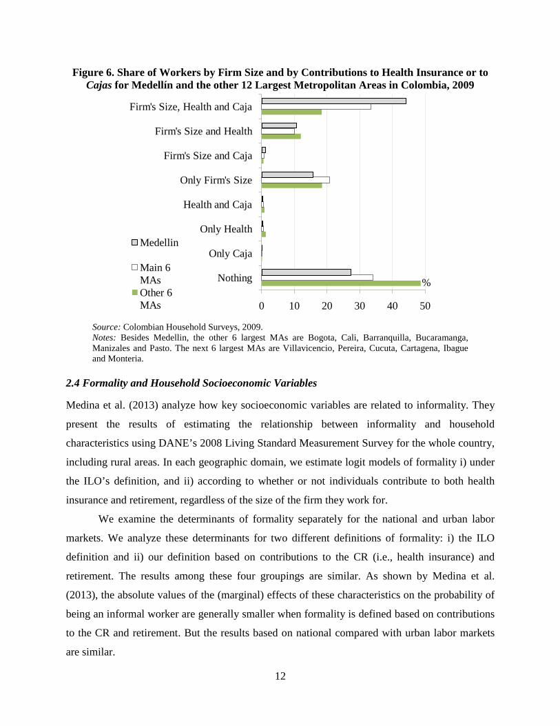
Figure 6. Share of Workers by Firm Size and by Contributions to Health Insurance or to Cajas for Medellín and the other 12 Largest Metropolitan Areas in Colombia, 2009
Source: Colombian Household Surveys, 2009. Notes: Besides Medellin, the other 6 largest MAs are Bogota, Cali, Barranquilla, Bucaramanga, Manizales and Pasto. The next 6 largest MAs are Villavicencio, Pereira, Cucuta, Cartagena, Ibague and Monteria.
2.4 Formality and Household Socioeconomic Variables Medina et al. (2013) analyze how key socioeconomic variables are related to informality. They
present the results of estimating the relationship between informality and household
characteristics using DANE’s 2008 Living Standard Measurement Survey for the whole country,
including rural areas. In each geographic domain, we estimate logit models of formality i) under
the ILO’s definition, and ii) according to whether or not individuals contribute to both health
insurance and retirement, regardless of the size of the firm they work for.
We examine the determinants of formality separately for the national and urban labor
markets. We analyze these determinants for two different definitions of formality: i) the ILO
definition and ii) our definition based on contributions to the CR (i.e., health insurance) and
retirement. The results among these four groupings are similar. As shown by Medina et al.
(2013), the absolute values of the (marginal) effects of these characteristics on the probability of
being an informal worker are generally smaller when formality is defined based on contributions
to the CR and retirement. But the results based on national compared with urban labor markets
are similar.
0 10 20 30 40 50
Nothing
Only Caja
Only Health
Health and Caja
Only Firm's Size
Firm's Size and Caja
Firm's Size and Health
Firm's Size, Health and Caja
%
Medellin
Main 6 MAsOther 6 MAs

13
Because this paper analyzes workers in an urban labor market, we focus on our results for
urban areas. Based on the ILO’s definition of informality (c.f., the results presented in column
vi), males are 16 percent more likely to work in the formal sector, and formality decreases with
age at an increasing rate (informality increases with age at an increasing rate, as Figure 7 shows).
Formality increases monotonically with education. Individuals with primary education are 18
percent more likely to work in the formal sector than those with no education. Workers with
incomplete secondary, complete secondary, incomplete higher, complete higher, and post higher
education are 28, 47, 58, 64 and 65 percent, respectively, more likely to work in the formal
sector than the uneducated.
The estimate of the interaction term between gender and years of education implies that,
other things being equal, males are less likely to work in the formal sector than females with the
same level of education, depending on how much more educated they are. Individuals attending
school are 6.5 percent more likely to work in the formal sector, while those born in urban areas
or who are heads of household (holding gender constant) are 3.9 and 6.3 percent more likely,
respectively, to work in the formal sector. Workers in small towns or rural areas are 5.5 and 14
percent less likely, respectively, to work in the formal sector. Finally, all geographic regions
have higher levels of informality than Bogota, the most informal being the Pacific, Atlantic,
Amazonia, and Orinoquia regions. In urban areas, individuals who receive rents from assets are
4.8 percent less likely to work in the formal sector, and those receiving subsidies are 11 percent
less likely (although this result does not necessarily reflect a causal relationship).
Core informality in Colombia is higher among older workers. As shown in Figure 7, core
informality rates of workers 55 years or older are above 50 percent for females and above 40
percent for males. Since many people frequently move between informal employment and
unemployment, it is worth noting that similarly, the sum of “core” informality + unemployment
rates of workers 55 years old or more is above 60 percent for females and above 50 percent for
males. The shaded areas refer to the population 21-54 years of age, the range for which impact of
US is assessed below.

14
Figure 7. Core Informality and Core Informality Plus the Unemployment Rate, by Age and Gender, Colombia’s 13 Largest Metropolitan Areas, 2009
Core Informality Core Informality + Unemployment.
Source: Colombian Household Surveys, 2009. Notes: The 13 largest MAs are Bogota, Medellin, Cali, Barranquilla, Bucaramanga, Manizales, Pasto, Villavicencio, Pereira, Cucuta, Cartagena, Ibague and Monteria.
In 2009, nearly one-half of Colombia’s workers were either unemployed or worked in the
core informal sector. Given the findings on the relationship been informality and educational
attainment, it is no surprise that unemployment and informality rates vary sharply by household
income. As shown in Figure 8, unemployment and informality rates are 28.3 and 50.4 percent,
respectively, in the poorest quintile of the household income distribution, compared to 5.3 and
19.7 percent, respectively, in the richest quintile. Taken together, these percentages imply that
more than three-quarters of workers in the poorest income quintile are either unemployed or
informal sector workers compared to only one-quarter of their counterparts in the richest income
quintile.
In Colombia, there is an important difference between wage earners and the self-
employed. As shown in Figure 9, most workers in the poorest income quintiles are self-
employed, while wage earners are concentrated mostly among the country’s richest individuals.
There are almost no wage earners who earn at least one minimum wage among individuals in the
first and second quintiles. In contrast, among individuals in the fourth and fifth quintiles, this
fraction is approximately equal to one-half.
0%
20%
40%
60%
80%
15-1
9
20-2
4
25-2
9
30-3
4
35-3
9
40-4
4
45-4
9
50-5
4
55-5
9
60-6
4
65+
Males
Females0%
20%
40%
60%
80%
15-1
9
20-2
4
25-2
9
30-3
4
35-3
9
40-4
4
45-4
9
50-5
4
55-5
9
60-6
4
65+
Males
Females

15
Figure 8. Core Informality and Core Informality plus the Unemployment Rate by Income Quintile, 2009
Source: GEIH Household Survey. Quintile based on per capita household income.
Figure 9. Share of Total Employment by Income Quintile. Wage Earners and Self-Employed, 1stQuarter, 2009.
Source: López (2010)
0%
10%
20%
30%
40%
50%
60%
70%
80%
1 2 3 4 5 TotalIncome Quintile
Unemployment Informality Unemployment+Informality
0%
20%
40%
60%
80%
100%
1 2 3 4 5
Self Employed Wage Earner Wage Earner, 1 Min Wage or More** Wage earners earning 1 minimum wage or more as a share of total workers in the income quintile.
Income Quintile

16
3. Duration of Unemployment Since 1999, Colombia has had one of the highest unemployment rates in the region, with
relatively long durations of unemployment.11 To analyze duration of unemployment, we used
data on workers who were employed in 2009 who, if they had previously been unemployed,
reported the duration of their last unemployment spell.12
Medina et al. (2013) present cumulative hazard functions using the 2009 Colombian
household survey at the national level for different populations according to gender, age,
economic sector, and category of worker, level of education, and geographic area. These
functions allow us to estimate the effects of different characteristics on the probability of leaving
unemployment by a given month.
The data reveal that male workers in Colombia remain unemployed for less time than
females. The largest difference between these groups takes place around the sixth month, when
74 percent of males and only 53 percent of females have found employment. Younger workers
also have shorter unemployment durations than older ones. By the 11th month, 85 percent of
workers under 18 have left unemployment compared to only 60 percent of those 55 to 64 years
of age.
Unemployment duration also varies across economic sectors. Workers in the economic
sectors of electricity, gas, and water have the shortest unemployment duration, while those in the
financial services sector have the longest. Seventy-two percent of workers in the former sector
have left unemployment by the fifth month, versus only 49 percent of those in the financial
sector.
The variation in unemployment duration by type of worker is also large. Employees in
rural areas are the ones with the shortest durations, followed by formal and informal employees
which are very similar, while employees working for the government have the longest
unemployment duration. Unemployment duration is less sensitive to variations in level of
education. The average duration of unemployment in urban areas (13 main MAs and
intermediate cities) is 10.6 months, while in the intermediate cities it is 10.9 months, and in rural
11 See Ball, De Roux, and Hofstetter (2011). 12 The estimates based on in this survey information may have a retrospective bias. It is well documented that survey respondents tend to underreport the incidence of periods of unemployment that occurred more than two year prior to the survey, particularly if these were short spells of unemployment.
17
areas it is 8.6 months.13 During the initial month, 14 and 20 percent of the unemployed
population found a job in the urban and rural areas, respectively. After three months, 44 percent
(54) of the urban (rural) unemployed had found some form of work. Two years later, only 10
percent of individuals were still looking for work in the urban sector and 7 percent in the rural
sector. We also compare unemployment duration in the three main metropolitan areas: Bogota,
Medellin, and Cali. Workers in Medellin spent longer periods of time unemployed than those in
Bogota, who in turn spent slightly longer time unemployed than those from Cali.
3.1 The Unemployment Subsidy Program The US program in Colombia was created in 2002 by Law 789, as a response to the large
unemployment rates that had persisted in the country since the late 1990s (c.f., Figure 1). It was
implemented starting with last quarter of 2003.14 Although this program was initially intended to
be implemented during critical economic downturns, it has operated continuously since its
creation.
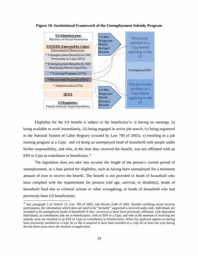
As shown in Figure 10, the US program is administered by the Social Protection Ministry
(MPS), and its funding is carried out through the Fund to Promote Employment and Protection to
the Unemployed (Fondo para el Fomento del Empleo y la Protección al Desempleado—
FONEDE). Three institutions jointly administer the program. The MPS establishes requirements
for i) eligibility, ii) maintenance of the benefits, and iii) the amount and duration of the benefit.
The Cajas operate and disperses payments to US recipients from FONEDE. The Family Subsidy
Superintendence (Superintendencia de Subsidio Familiar—SSF) is responsible for program
supervision and oversight.
FONEDE is funded using revenues from the 4 percent payroll tax and its corresponding
yields.15 Thirty-five percent of FONEDE’s resources are used to pay unemployment benefits.
This benefit is provided only to unemployed heads of household. The grant is an in-kind benefit
equal to one and a half legal minimum (monthly) wages, divided into six equal monthly
payments. This benefit is awarded through contributions to the health system, meal tickets, or
13 The intermediate cities are all those cities smaller than the main 13 MAs but still urban. 14 See also regulatory decrees 827 of April 2003, 2340 of August 2003, 3450 of December 2003, and 586 of March 2004. 15 According to Law 920 of 2004, the non-executed resources during the relevant fiscal term are transferred to the Low-Income Housing Fund (Fondo Obligatorio para el Subsidio Familiar de Vivienda de Interés Social—FOVIS).

18
educational bonds, according the beneficiary’s choice. This benefit does not depend on the
number of people in the household.
Even though the magnitude of the benefit of the US program seems at first small, it
equals nearly 100 (40) percent of the 2005 baseline (before treatment) earnings of informally
employed female (male) beneficiaries, and about 50 (30) percent of the 2005 baseline earnings of
female (male) formally employed beneficiaries. This is a reasonable amount given that, as
Nicholson and Needless (2006) affirm, for most states in the United States, the maximum benefit
is usually between 50 and 70 percent of earnings, with a more typical replacement rate equaling
about 47 percent of prior earnings.
The target population of this benefit is jobless heads of household who were enrolled in a
Caja while they were employed. Accordingly, 30 percent of FONEDE’s resources serve
unemployed heads of household with previous affiliation to a Caja, and 5 percent to those
without previous affiliation to a Caja.
An additional 25 percent of FONEDE’s resources are allocated to training programs for
beneficiaries who previously contributed to a Caja, although the National Learning Service
(SENA) has resources to provide training programs to the unemployed, regardless of whether
they have previously contributed to a Caja.16 The objective of the training program is to increase
the possibility of employment among beneficiaries through better qualification and support of
their job search. The training program is discretionary, and is offered by each Caja according to
its criteria, operational schemes, and management.17
16 Articles 10 and 12, Law 789of 2002. 17 Since the Cajas offer those services for their enrollees, the US guarantees that the former beneficiaries of the Cajas, once unemployed, can keep their services.
19
Figure 10: Institutional Framework of the Unemployment Subsidy Program
Eligibility for the US benefit is subject to the beneficiary’s: i) having no earnings; ii)
being available to work immediately, iii) being engaged in active job search; iv) being registered
in the National System of Labor Registry (created by Law 789 of 2002); v) enrolling in a job
training program at a Caja; and vi) being an unemployed head of household with people under
his/her responsibility, and who, at the time they received the benefit, was not affiliated with an
EPS or Caja as contributor or beneficiary.18
The legislation does not take into account the length of the person’s current period of
unemployment, or a base period for eligibility, such as having been unemployed for a minimum
amount of time to receive the benefit. The benefit is not provided to heads of household who
have complied with the requirements for pension (old age, survival, or disability), heads of
household fired due to criminal actions or other wrongdoing, or heads of household who had
previously been US beneficiaries. 18 See paragraph 5 of Article 13, Law 789 of 2002, and Decree 2340 of 2003. Besides verifying social security participation, the information which does not need to be “formally” supported is received under oath. Individuals are accepted to be unemployed heads of household if they can prove to have been previously affiliated, with dependent individuals, as contributors and not as beneficiaries, with an EPS or a Caja, and who at the moment of receiving the subsidy were not enrolled in an EPS or Caja as contributors or beneficiaries. When the applicant applies as having been previously enrolled in a Caja, he or she is required to have been enrolled in a Caja for at least one year during the last three years since the moment of application.
UI Administrator:Ministry of Social Protection
UI Regulator:Family Subsidy Superintendency
FONEDE (Operated by Cajas)Destination of Resources:
* Administration (5%)
* Unemployment Benefits for HH Previously in Caja (30%)
* Unemployment Benefits for HH Previously Not in Caja (5%)
Previously enrolled in a Caja before
applying to the UI
1/4 Min Wages per Month during 6 Months
Not previously enrolled in a Caja before
applying to the UI
* Training Programs (25%)
* Microcredit Programs (35%)
Unemployed HH
1/4 Min Wages per Month during 6 Months
SENA

20
Among US beneficiaries, reasons for losing the right to benefits include the following:
when the beneficiary becomes employed, has rejected an acceptable job offer according to
his/her academic qualifications, has been drafted into compulsory military service, receives other
type of work remuneration, is incarcerated, has a retirement plan, or dies.
Finally, 35 percent of FONEDE’s resources are used for microcredit programs, and 5
percent for the fund’s administration. The Cajas spend their administrative funds in carrying out
activities related to distribution of subsidies, such as promotion of the US, reception of
applications, verification of compliance with requirements (activity performed through
information crossing of applicants with other Cajas and the social security system, carried out by
the Cajas’ national association representing all the Cajas of the country). Their activities also
include providing the in-kind benefit chosen by US beneficiaries (i.e., food, educational, or
health support) and verifying compliance with the program’s requirements.
3.2 Statistics on the Unemployment Subsidy Program and Workforce Training Nationally, the unemployment rate among heads of household, US’s target population, has
varied around 6 percent in 2003, 2004, and 2009, and about 5.5 percent for the rest of the period
(c.f., Table 1). In Medellin, the unemployment rate has averaged around 7.6 percent. By the
second quarter of 2009, the number of unemployed heads of household at the national level
reached 611,000, and in Medellin it reached 65,000.19 The last row of Table 1 shows the ratio
between the number of US program subsidies allocated and the number of unemployed heads of
household. Between 2004 and 2009, the program covered an average of 16.6 percent of
unemployed heads of household at the national level, and 23.4 percent in Medellin.
The US program is relatively small in size. In 2008, expenditures amounted to
approximately 153,000 million Colombian pesos (COP), or about 0.04 percent of Colombia’s
GDP.20 This percentage is small when compared the United States’ unemployment insurance
program, which according to Nicholson and Needels (2006) was about $34 billion in 2004, or
nearly 0.23 percent of that nation’s GDP.
Program records show that the training benefit has not been fully used. Additionally, it
has had a dropout rate of 20 percent. Nonetheless, most beneficiaries who previously contributed
19 At that time, there were 2.37 million unemployed at the national level, 265,000 of whom resided in Medellin. 20 See Carrasco (2009) for more details. The average exchange rate between 2005 and 2006 was US$2,340.
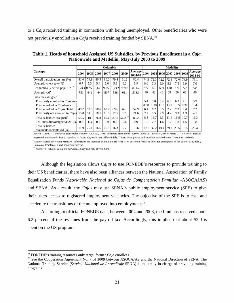
21
to a Caja received training in connection with being unemployed. Other beneficiaries who were
not previously enrolled in a Caja received training funded by SENA.21
Table 1. Heads of household Assigned US Subsidies, by Previous Enrollment in a Caja, Nationwide and Medellín, May-July 2003 to 2009
Although the legislation allows Cajas to use FONEDE’s resources to provide training to
their US beneficiaries, there have also been alliances between the National Association of Family
Equalization Funds (Asociación Nacional de Cajas de Compensación Familiar –ASOCAJAS)
and SENA. As a result, the Cajas may use SENA’s public employment service (SPE) to give
their users access to registered employment vacancies. The objective of the SPE is to ease and
accelerate the transitions of the unemployed into employment.22
According to official FONEDE data, between 2004 and 2008, the fund has received about
6.2 percent of the revenues from the payroll tax. Accordingly, this implies that about $2.0 is
spent on the US program.
21 FONEDE’s training resources only target former Caja enrollees. 22 See the Cooperation Agreement No. 7 of 2009 between ASOCAJAS and the National Direction of SENA. The National Training Service (Servicio Nacional de Aprendizaje-SENA) is the entity in charge of providing training programs.
2004 2005 2006 2007 2008 2009Average 2004-09 2004 2005 2006 2007 2008 2009 Average
2004-09Overall participation rate (%) 81.0 79.9 80.5 80.3 79.4 81.2 80.4 74.5 72.3 72.2 72.8 72.0 74.9 73.1Unemployment rate (%) 6.7 5.3 5.4 5.6 5.8 6.3 5.9 8.0 7.3 8.0 5.9 7.5 8.9 7.6Economically active pop., EAP♦ 8,243 8,259 8,671 9,050 9,242 9,708 8,862 577 579 599 650 670 726 634Unemployed♦ 551 441 464 507 536 611 518.3 46 42 48 38 50 65 48Subsidies assigned♦
Previously enrolled in Comfama 5.4 5.0 5.4 6.0 6.3 7.1 5.9Prev. enrolled in Comfenalco 0.68 1.20 1.10 1.20 1.65 2.32 1.4Prev. enrolled in Cajas Total 49.7 59.5 58.6 63.7 69.6 46.3 57.9 6.1 6.2 6.5 7.2 7.9 9.4 7.2Previously not enrolled in Cajas 15.8 51.3 18.1 16.9 17.5 9.9 21.6 2.7 9.5 2.9 4.2 3.9 1.3 4.1Total subsidies assigned* 65.5 110.8 76.8 80.6 87.1 56.2 ** 86.2 8.8 15.7 9.3 11.4 11.8 10.7 11.3Tot. subsidies assigned/EAP (%) 0.8 1.3 0.9 0.9 0.9 0.6 0.9 1.5 2.7 1.6 1.7 1.8 1.5 1.8Total subsidies assigned/Unemployed (%) 11.9 25.1 16.6 15.9 16.3 9.2 16.6 19.1 37.2 19.4 29.7 23.5 16.5 23.4
Colombia MedellínConcept
Source: DANE – Continuous Households Survey (2003-05), Great Integrated Households Survey (2006-09). Mobile Quarter Series 01 - 08. Note: Resultsexpressed in thousands. Due to rounding in thousands, totals may differ slightly. ♦ EAP, Unemployed and subsidies assigned are in Thousands, and only *Source: Social Protection Ministry (Information on subsidies at the national level is on an annual basis; it does not correspond to the quarter May-July),Comfama, Comfenalco, and household surveys.** Number of subsidies assigned between January and July of year 2009.

22
However, these data also show that through 2008, resources appropriated for these
programs have not been fully spent.23 Total expenditures on US benefits have approached the
legal limit. Of the 35 percent of FONEDE’s resources budgeted annually for US benefits, the
Cajas have spent more than 96.5 percent. In contrast, the microcredit program has spent less than
50 percent of what was intended under the legislation. Since 2005, the Cajas’ microcredit
expenditures have been about 30 percent of FONEDE’s budgeted resources.
Data from the final quarter of 2003 through July 2009 indicate that there have been
495,078 US claimants. Of this total, 72.5 percent were allocated to heads of household with prior
Caja enrollment, and the remaining 27.5 percent to heads of household without prior Caja
enrollment. During this period, female heads of household received a larger proportion of
FONEDE allocations of US benefits than males. Women received about 290,000 (or 58.6
percent) of these allocations compared with 205,000 (or 41.4 percent) for men.
Administrative records show that US beneficiaries chose to receive their benefits almost
entirely in the form of food vouchers. They opted for this modality 97.8 percent of the time. The
other modalities, health and education, were chosen by 1.7 and 0.5 percent of beneficiaries,
respectively.
The program’s administrative records also indicate that the wait time for the unemployed
to receive US benefits varied considerably. Depending on the unemployed state and whether they
had previously been a member of a Caja, these times varied from between two months
(minimum wait time recorded) and 19 months (maximum wait time). On average, people with no
previous enrollment in Cajas had longer wait times, mainly in small states, where it took
beneficiaries 26 months in 2007; 28 months in 2008; and 27 months during the first six months
of 2009. In contrast, applicants with previous enrollment in Cajas showed shorter wait times,
ranging between two and eight months, the lowest being those in the smaller states.24
Most US beneficiaries have been under 45 years of age: 35-44 year olds are 36.9 percent
of beneficiaries, and 25-34 year olds make up 28.3 percent of beneficiaries. In contrast, 45-54
year olds constitute only 21.2 percent of beneficiaries.25 Young adults and youths are
underrepresented among US beneficiaries, even though young people constitute a
23 As was discussed above, FONEDE’s non-executed resources during each fiscal year are transferred to FOVIS. 24Medellin is located in Antioquia, which is classified as a large state. 25 Data from 2005 to June 2009.

23
disproportionate share of the unemployed. This underrepresentation arises by design because
young people are less likely than other unemployed persons i) to be heads of household or ii) to
have previously enrolled in a Caja. Likewise, the oldest unemployed also are underrepresented
among US, because they are often eligible to receive benefits from a retirement plan.
Administrative records for the program show a difference between distributions of
resources according to whether US beneficiaries were previously enrolled in a Caja and their
prior education. For beneficiaries previously enrolled in a Caja, the highest concentration of
resources was seen in people who had finished secondary school, followed by people who only
finished primary school or had no education. For beneficiaries with no previous enrollment,
more than 70 percent of the subsidies were distributed to people with no education, or no more
than primary school.
As is to be expected from the use of prior enrollment in a Caja as an indicator of
formality, these workers were better paid prior to becoming unemployed compared with their
peers who had not been members of a Caja. Among people with previous Caja enrollment and
who received US benefits during the 2003 to 2009 period, the wages of 77 percent of them
ranged from between 1 and 2 minimum wages. In contrast, among people with no prior Caja
enrollment, who received US benefits during the 2003 to 2009 period, 90.8 percent had earned
less than the minimum wage.
Information about resources distributed to applicants with or without previous enrollment
in a Caja, disaggregated by state, indicates that greater provisions to beneficiaries previously
enrolled in a Caja, near to 85 percent, were provided by Cajas from the states of Caldas, Cesar,
Cauca and Casanare. Those who received less than 50 percent were Cajas from Choco, Sucre,
Amazonas, and Arauca. Antioquia, the state where Medellin is located, allocated 77 percent to
beneficiaries with previous enrollment in Cajas (See Medina et al., 2013).26
26 If Cajas executed all their available resources to fund subsidies, the share for those beneficiaries previously enrolled in a Caja would be the share of resources located by FONEDE to beneficiaries previously enrolled to a Caja (30 percent) divided by the total share of resources located to beneficiaries (35 percent), that is, 30/35 ≅ 85.7. However, Cajas usually execute less of one or other type of subsidy, thus explaining the observed variation in the percentages shown in Medina et al. (2013).
24
4. Impact Evaluation 4.1 Establishing Eligibility for the Unemployment Subsidy As explained above, enrollment in a Caja is closely linked to formality. Formal workers are
defined as potential beneficiaries who are unemployed heads of household and who have
contributed to any Caja for at least one year during the previous three years before losing their
jobs. Informal workers are defined as potential beneficiaries who were unemployed heads of
household without earnings and who did not contribute to a Caja for at least one year during the
previous three years.27
According to these definitions, easily observable characteristics like age, education,
marital status, household size, and others are not directly used to target eligibility for the US.
Nonetheless, self-selection generates differences in those characteristics among beneficiary and
non-beneficiary populations.
An additional requirement of the US program is that in order to receive US benefits, the
claimant may not be a current beneficiary or a contributor to an EPS or to a Caja. Policy makers
imposed this restriction to prevent employed workers from applying for and obtaining the US
benefit. Because Colombian law requires employers either i) to enroll their employees in the
Contributive Regime and in a Caja, or ii) to enroll in the CR themselves, this requirement allows
the Cajas to prevent free-riding by employed individuals.
This restriction also seeks to target the US benefit to the most vulnerable part of the
unemployed population. Anyone enrolled in an EPS or Caja who indicated that he or she or a
member of his household could be enrolled.28 This limitation implies that unemployed informal
workers who wanted to claim US benefit, but who had enrolled in the CR on their own, would
have to stop contributing to the CR. In contrast, had they enrolled in the SR rather than in the
CR, this same person could have applied for a US benefit. As shown in Table 2, between 2003
27 Among these informal workers, the program gives priority to artists, sportsmen, and writers. That is, anyone in this group would become beneficiary before other comparable candidates from other professions who applied with the same date (Paragraph 2 of Article 13 of Decree 2340 of 2003). 28Paragraph 5º, Article 13 of Law 789, 2002. As explained by Synergia (2009), this requirement is enforced by some of the most important Cajas.

25
and October 2009, nearly 20 percent of US claimants were either denied or lost their US benefits
because they had been enrolled in an EPS (CR).29
The importance of this no EPS/no CR requirement becomes even more apparent once we
understand how Colombia targets health insurance for the poor through the Subsidized Regime
(SR). Prior to 1993, only workers affiliated with the Colombian Institute of Social Insurance,
ISS, were beneficiaries of privately provided health insurance, while uninsured individuals were
treated by the network of public hospitals. In 1993, Law 100 established two tiers of health
insurance: the Contributive Regime (CR) and the Subsidized Regime (SR). The CR covers
formal workers with a comprehensive set of health services and pays for treatment for nearly all
of the most common illnesses. The SR covers the poorest informal workers with a plan that
encompasses about 55 (initially 50 percent) of the illnesses covered by the CR. Formal workers
and their employers fund workers’ insurance premiums for coverage by the CR. Several public
funds (national transfers, municipalities’ budgets, lottery contributions, etc.) and the Solidarity
Fund, FOSYGA, collect resources to fund the SR.
Table 2. Reasons for Which Unemployed Applicants are Denied or Lose the Right to Receive US Benefits
Source: Ramírez (2009). * Includes beneficiaries contributing their own resources or those of a third party.
A key aspect of the 2003 US reform is its requirement that potential beneficiaries not be
beneficiaries of the CR regime. In addition, this restriction interacts with the existing way that
policy establishes eligibility for the SR. To target people for the SR, officials first interview
about 70 percent of the poorest households. Secondly, using the data gathered from these 29 Ramírez (2009) uses only information on applicants and beneficiaries of Comfama, one of the two Cajas operating in Medellín.
N % N % N % N % N % N % N % N %Enrolled in any Caja 71 48 606 41 1,725 50 1,596 59 1,585 68 732 69 2,256 51 1,289 54Resigned the benefit/becomes employed 7 5 51 3 343 10 382 14 334 14 80 8 289 6 221 9
Beneficiary of EPS* 54 36 821 55 909 26 438 16 297 13 166 16 596 13 486 21Other 16 11 18 1 487 14 289 11 125 5 88 8 1,311 29 371 16Total 148 100 1,496 100 3,464 100 2,705 100 2,341 100 1,066 100 4,452 100 2,366 100Benefits for Previously: 1,472 7,845 10,893 8,355 9,442 10,961 9,330 8,595
Enrrolled in Caja 749 6,690 6,804 7,230 7,804 8,617 7,977 6,781Not Enrrolled in Caja 723 1,155 4,089 1,125 1,638 2,344 1,353 1,814
Rejection Rate (%) 10.1 19.1 31.8 32.4 24.8 9.7 47.7 26.4
Oct 2009 AverageReason 2003 2004 2005 2006 2007 2008

26
interviews, they construct a welfare index. Finally, officials used this index—known as a
“SISBEN score” to classify households into one out of six levels. Only households classified in
the two lowest levels of SISBEN scores were eligible to become beneficiaries of the SR.
Additionally, any household that was a beneficiary of the CR could not become a beneficiary of
the SR.
As observed by Camacho and Conover (2008), there are beneficiaries of the SR at both
sides of the SISBEN cutoff score. This point occurs between levels two and three. But the share
of beneficiaries changes discontinuously at this score. In theory, knowing that enrollment in the
SR changes discontinuously at this threshold does not guarantee that the percentages i) of non-
CR beneficiaries or ii) of US beneficiaries also change discontinuously at this cutoff score.
Nonetheless, because households at SISBEN levels one and two are more likely to benefit from
the SR than those in levels three or above, the expected benefit of being a beneficiary of the CR
should be lower for households to the left the threshold than for those to the right of it.
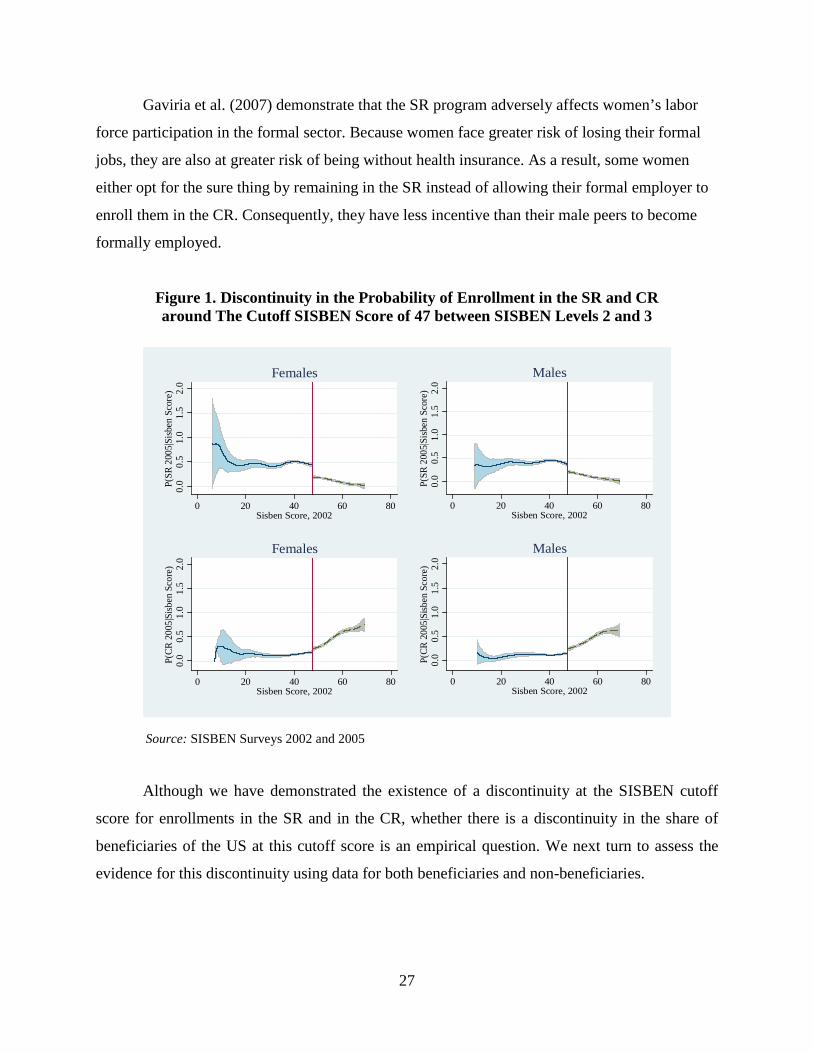
We find evidence of the foregoing relationship in our data. The graphs at the top of
Figure 11 show the 2005 probability of enrollment in the SR as a function of individuals’ 2002
SISBEN score. The graphs at the bottom of the figure show the probability of enrollment in the
CR. The graphs include a vertical line at the “cutoff” score of 47 between SISBEN levels 2 and
3.
As shown by Figure 11, the probability of enrollment in the SR (CR) declines (increases)
discontinuously at the cutoff. Below we illustrate the change in the probability of US enrollment
around the cutoff.
There is anecdotal evidence that some formerly informal workers who became formal
employees have asked their employers not to enroll them in the CR so that they would not lose
their affiliation in the SR, and there is quantitative evidence that the SR decreases formality by
almost 4 percent.30 This type of situation is more likely when the worker’s formal job is less
stable. These workers recognize that if they lose their job, they have to reapply to the SR and
would not be covered for any health insurance until the government enrolls them in the program
again.
30 See Camacho et al. (2009)
27
Gaviria et al. (2007) demonstrate that the SR program adversely affects women’s labor
force participation in the formal sector. Because women face greater risk of losing their formal
jobs, they are also at greater risk of being without health insurance. As a result, some women
either opt for the sure thing by remaining in the SR instead of allowing their formal employer to
enroll them in the CR. Consequently, they have less incentive than their male peers to become
formally employed.
Figure 1. Discontinuity in the Probability of Enrollment in the SR and CR around The Cutoff SISBEN Score of 47 between SISBEN Levels 2 and 3
Source: SISBEN Surveys 2002 and 2005
Although we have demonstrated the existence of a discontinuity at the SISBEN cutoff
score for enrollments in the SR and in the CR, whether there is a discontinuity in the share of
beneficiaries of the US at this cutoff score is an empirical question. We next turn to assess the
evidence for this discontinuity using data for both beneficiaries and non-beneficiaries.
0.0
0.5
1.0
1.5
2.0
P(SR
200
5|Sisb
en S
core
)
0 20 40 60 80Sisben Score, 2002
Females
0.0
0.5
1.0
1.5
2.0
P(SR
200
5|Sisb
en S
core
)
0 20 40 60 80Sisben Score, 2002
Males
0.0
0.5
1.0
1.5
2.0
P(CR
200
5|Si
sben
Sco
re)
0 20 40 60 80Sisben Score, 2002
Females
0.0
0.5
1.0
1.5
2.0
P(CR
200
5|Si
sben
Sco
re)
0 20 40 60 80Sisben Score, 2002
Males

28
4.2 Data Two sources of data were used to evaluate the impact of the US. One was provided by two
Cajas: Comfama and Comfenalco. These are the only Cajas that operate in the state of
Antioquia, a state with a population of nearly 6 million people. The state’s capital is Medellin.
Data provided by Comfama includes 47,600 heads of household who were US beneficiaries.
These Caja participants received US benefits at some point between September 2003 and
December 2009. Data provided by Comfenalco include nearly 23,000 individuals. These Caja
participants received US benefits at some point between February 2004 and December 2008.
The second source of data is successive population censuses from SISBEN surveys of
Medellin for 2002, 2005, and 2009.31 The SISBEN data set is not a panel of households. Rather,
it consists of three cross-sections from a census of roughly the poorest 70 percent of the
population. To create a panel data set, we matched household records across the three years.32
As shown by Medina et al. (2013), although the 2002 SISBEN survey was implemented
around 1994, most individuals were interviewed in 2002. Between 2003 and 2005, the country
updated the methodology used to estimate the SISBEN score, which determines eligibility for
social benefits, and then updated information for all individuals in 2005 and 2009. Our final
sample of beneficiaries consists of 6,004 beneficiaries who were matched to both the 2002 and
2005 SISBEN surveys and 14,364 beneficiaries who were matched to both the 2005 and 2009
SISBEN surveys.33
It is important to highlight that the information contained in the SISBEN survey is used to
calculate the SISBEN score, based on which households are classified in one out of six SISBEN
levels. Individuals belonging to SISBEN levels 1 or 2 become eligible to be enrolled in the
Subsidized Regime, as was explained above, but they are not automatically enrolled.
The survey includes a question on whether individuals are enrolled in the SR or the CR.
We use that question to determine whether these individuals were CR beneficiaries in the
31 The SISBEN data for Medellin are available every three months. Nonetheless, they are only rarely updated by the households (see more below). The data might become valuable if we were to use SISBEN data much closer to the moment that individuals enroll in the program. However, the endogenous updating of information would pose additional challenges to identification. 32 We assign an identification number to each household member to do the match. 33 See Medina et al. (2013) for additional details of the way our final sample was constructed.

29
baseline years, 2002 and 2005 and in the follow-up years, 2005 and 2009.34 By matching the
Cajas data with the SISBEN data, we have information on US beneficiaries and non-
beneficiaries at three points in time.
Figure 12 shows the timeline considered in our exercise. We use 2002 SISBEN survey
for our baseline data, which takes place at t0 in the figure. Individuals enroll into the
unemployment subsidy at T, which we know from data provided by the Cajas. Then we observe
individuals again in the 2005 SISBEN survey, which takes place at t1 in the figure (Period 2002-
2005).35
Figure 12. Timing of the Key Events and Data Used at Each Moment
Similarly, we use 2005 SISBEN survey for baseline data and the 2009 SISBEN survey as follow-
up for those individuals enrolled into the unemployment subsidy at T, between those two dates
(Period 2005-2009) as shown in Figure 13.
Figure 13. Timing of the Key Events and Data used at Each Moment
34 The few observations of the 2005 SISBEN survey not collected in 2005 are of people who asked the municipality of Medellin to update their information. Note that only households whose standard of living deteriorated would be willing to ask for a new interview to update their status and lower their SISBEN score. The same is true for people whose data was not collected in 2002 but between 2003 and 2004. All individuals in the last round were interviewed in a short period of time between late 2009 and early 2010. 35 We use SISBEN survey for Medellin (the second-largest city in Colombia) because the data provided by the Cajas (Comfama and Comfenalco), only cover municipalities of Antioquia. Among the subsidies granted by these two Cajas, a large share of those, were for people who at the moment of the subsidy were living in Medellin.
Baseline(2002 Sisben Survey)
Enrollment into UI.(CCFs and 2002 Sisben
Survey)
:0t T: :1tFollow-up
(2005 Sisben Survey)
Baseline(2005 Sisben Survey)
Enrollment into UI.(CCFs and 2005 Sisben
Survey)
:0t T: :1tFollow-up
(2009 Sisben Survey)

30
To clarify the content of these figures, first note that the subsidy lasts for six months after
enrollment, for which we exclude from the sample those beneficiaries who were matched to the
SISBEN survey less than six months after their enrollment. Second, to limit the possibility of
outcomes being affected by other interventions different from the US, we limit the length of time
between the baseline and enrollment in the US, and we also focus on the impacts of the program
in a limited period of time, namely within 1.5 years after they exit from the US program. Thus,
we exclude from the sample those beneficiaries whose differences in time, between the date of
enrollment and both, the baseline and follow up (plus six months of subsidy) are larger than 24
months. That is, we exclude those for whom,
monthstT 240 >−
monthsTt 241 >−
However, we repeat the exercises that will be presented later, covering only 18 months in order
to assess the robustness of the results.36
Third, there may be differences between the way individuals present themselves as heads
of household to the Cajas and the way they self-classify as such in the SISBEN survey, or their
parenthood status may change between the time they were interviewed for the SISBEN survey
and the time they enrolled in the US. To address this issue, first, we separately estimate the
impacts of the US for men and women. Second, we use as a comparison group people selected
from the whole sample of men (or women) at the baseline years (2002 or 2005), in case
beneficiaries were heads of household at the moment they enrolled in the US, but not necessarily
at the baseline or follow up (2005 or 2009 respectively). Third, alternatively we use as a
comparison group those who were heads of household at the baseline.
4.3 Outcomes Studied The SISBEN survey includes key outcomes of interest for this evaluation; these outcomes are
available for both of the baseline surveys, 2004 and 2007 and both of the follow up surveys,
2007 and 2009. The outcomes that we use are the following:
36 Those exercises are available upon request but are not included in this article.
31
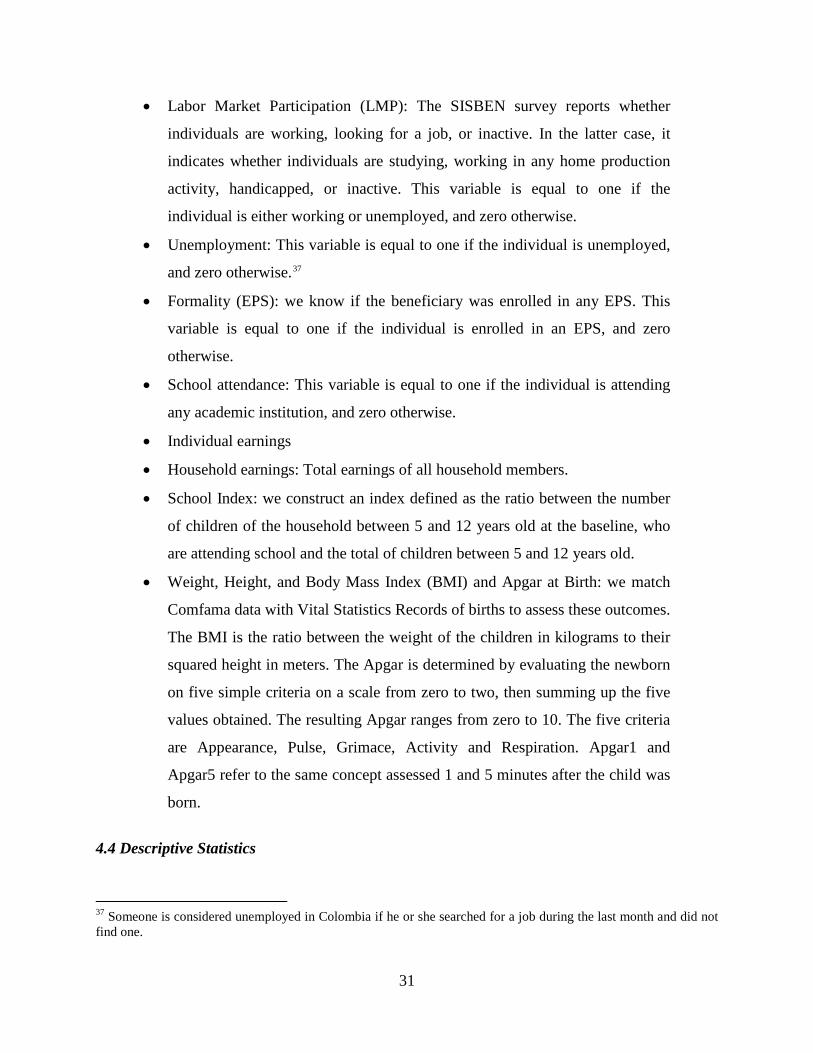
• Labor Market Participation (LMP): The SISBEN survey reports whether
individuals are working, looking for a job, or inactive. In the latter case, it
indicates whether individuals are studying, working in any home production
activity, handicapped, or inactive. This variable is equal to one if the
individual is either working or unemployed, and zero otherwise.
• Unemployment: This variable is equal to one if the individual is unemployed,
and zero otherwise.37
• Formality (EPS): we know if the beneficiary was enrolled in any EPS. This
variable is equal to one if the individual is enrolled in an EPS, and zero
otherwise.
• School attendance: This variable is equal to one if the individual is attending
any academic institution, and zero otherwise.
• Individual earnings
• Household earnings: Total earnings of all household members.
• School Index: we construct an index defined as the ratio between the number
of children of the household between 5 and 12 years old at the baseline, who
are attending school and the total of children between 5 and 12 years old.
• Weight, Height, and Body Mass Index (BMI) and Apgar at Birth: we match
Comfama data with Vital Statistics Records of births to assess these outcomes.
The BMI is the ratio between the weight of the children in kilograms to their
squared height in meters. The Apgar is determined by evaluating the newborn
on five simple criteria on a scale from zero to two, then summing up the five
values obtained. The resulting Apgar ranges from zero to 10. The five criteria
are Appearance, Pulse, Grimace, Activity and Respiration. Apgar1 and
Apgar5 refer to the same concept assessed 1 and 5 minutes after the child was
born.
4.4 Descriptive Statistics
37 Someone is considered unemployed in Colombia if he or she searched for a job during the last month and did not find one.

32
Medina et al. (2013) present descriptive statistics of the variables from the SISBEN survey that
we use in our matching estimations. Some of these variables are school attendance, earnings of
household, earnings of the individual, labor market participation, unemployment, gender of the
head of household, number of children under 6 and 18 years old, household size, and others.
They also include a panel with the descriptive statistics for the complete sample of individuals
who became US beneficiaries between 2002 and 2005, and another panel for non-beneficiaries
during the same period. They include information for females and males, and for formal and
informal workers, by gender, as well as the mean and standard deviation of the outcomes of the
individuals based on the information included in the 2005 SISBEN survey, and their baseline
characteristics from the 2002 SISBEN survey.
According to the baseline information, non-beneficiaries are better off than beneficiaries,
contrary to the finding by Mazza (2000) who found that unemployment insurance beneficiaries
from several countries she analyzed—including Argentina, Barbados, and Brazil—are middle-
income workers rather than poor workers. She reported that unemployment insurance
beneficiaries in these countries had higher rates of school attendance, higher household and
individual earnings, and lower unemployment rates. Additionally, they were more likely to have
secondary education, their households were less likely to be headed by a woman, have fewer
children under 6 and 18, have fewer members, were less likely to own the house they live in, and
were less likely to live in socioeconomic stratum 1 (i.e., the poorest stratum).38
Similar conclusions are arrived at by studying the results of the whole sample for the
period between 2005 and 2009 and from the statistics for individuals who were heads of
household during the baseline years.
4.5 Identification Strategy and Estimation In this section we propose several different ways to identify the effects of the US program on a
variety of outcomes. Each method solves the selection problem in a different way. The
38 Urban areas in Colombia are split into six socioeconomic strata in which the first has the lowest income levels (the poorest). The strata are used by authorities to spatially target social spending like that in the supply of public services (water, electricity), housing, health insurance for the poor, etc. Note that socioeconomic stratification is assigned to the housing units, and it is a method of spatial targeting which is a function of the housing characteristics and its amenities, while the SISBEN levels are assigned to the households, and it is a function of the household and housing characteristics.

33
estimators that we consider are based on i) regression discontinuity designs (RDD), ii) matching
difference-in-differences estimators, and iii) matching cross-sectional estimators.
In what follows we will refer to the impact of the “treatment on the treated” as our
parameter of interest. Treatment status is denoted by the binary variable D, D=1 for treated
individuals, and D=0 for untreated individuals.
The untreated individuals comprise the comparison group. We estimate the effect of D on
an outcome Y, whereY1 denotes the treated outcome and Y0 denotes the untreated outcome. After
we condition on a set of observed variables X, we define the impact of the treatment on the
treated as follows: TT=E(Y1-Y0|D=1,X).
4.6 Regression Discontinuity Design RDD is an appropriate identification strategy whenever assignment to treatment is based on
individuals’ score on a continuous variable, and also when those individuals with a score at or
below a clearly defined cutoff are more likely to become enrolled that those whose scores fall
beyond that cutoff. Since individuals’ characteristics change continuously along the assignment
variable, individual characteristics on both sides of the cutoff are nearly identical. The only
difference (in the limit) between the two groups around the cutoff score is on whether or not it is
likely they enrolled in or received the treatment. This design allows the evaluator to use
individuals close to the cutoff score as if they were drawn from an experimental design.
The targeting of the SR implies that the probability of enrollment to the SR, and to the
CR, changes discontinuously at the cutoff between SISBEN levels 2 and 3. Since the US requires
its applicants not to be enrolled in the CR, in this section we assess whether this requirement is
also implying a discontinuity in the enrollment to the US at the cutoff between SISBEN levels 2
and 3, in order to apply RDD to identify the impact of the US on a subset of outcomes around the
cutoff point.
4.7 Strategy First, let us analyze how this approach allows us to identify the impact of the US for individuals
whose SISBEN score is close to the cutoff score. According to this approach, selection for
treatment depends either deterministically or probabilistically on a continuous variable z, the
SISBEN score, so that either we say that the design is sharp because selection for treatment is

34
determined deterministically as a function of z, and changes discontinuously at the cutoff z0; or
the design is fuzzy because selection for treatment changes probabilistically, and the probability
of treatment changes discontinuously at the cutoff score.
In this context, the outcome Y can be expressed as a function of the treatment D and the
controls X: Yi = α⋅Xi + β⋅Di. Note that β identifies the impact of the US only around the cutoff
score. So this regression is run locally using only treated and untreated individuals whose
SISBEN score is close to the cutoff score.
We now provide empirical evidence that supports the standard assumptions required in an
RDD. According to our rationale, the system used to target the SR regime, coupled with the
eligibility requirements for US claimants, implies that probability of enrollment into US should
change discontinuously at the cutoff between SISBEN levels two and three. This threshold
determines the boundary between the eligible and non-eligible population to the SR. This test
would ensure that assumption (i) above is satisfied.
Figures 14 and 15 show local linear regressions of estimates of the probability of
enrollment in the US conditional on the SISBEN score. For these figures, we use data for
individuals who became beneficiaries between 2002 and 2005 and matched them to their
responses in 2002 (baseline) and 2005 (follow-up) SISBEN surveys. The analysis depicted in the
figures is based on samples restricted to individuals whose outcomes are observed in the 2005
SISBEN survey (t1), two years after the enrollment date in the US (T), that is, as given above,
individuals for whom t1 - T< 24 months.
The figures include results for the sample of formal and informal individuals according to
two alternative definitions of formality. (See Table 3) Administrative data provided by the Cajas
allow us to know whether or not US beneficiaries were previously enrolled in a Caja, or in an
EPS. In contrast, for individuals in the comparison group, the SISBEN survey data do not allow
us to know whether individuals in the baseline were enrolled in a Caja, but only whether they
were enrolled in an EPS. This distinction explains why we consider two groups of formal
individuals: one (A in the table) we denote “EPS” that takes as formal anyone who was enrolled
in an EPS in the 2002 SISBEN survey (baseline), regardless of whether he or she was enrolled in
a Caja. A second group (B in the table) we denote “Caja” that takes as formal in the treatment
group (US beneficiaries) only those who were enrolled in a Caja at the baseline, whereas
formality in the comparison group are those previously enrolled in an EPS.

35
The four graphs at the top of Figure 14 summarize our results for females. The two
graphs at the top assess the discontinuity for the samples of females employed in the formal
sector based on previous enrollment in the EPS (left) or the Caja (right). The two graphs at the
bottom assess the discontinuity of informally employed females based on the same respective
definitions. The four graphs at the bottom include the same information for females, but with the
additional restriction that individuals had enrolled in the US within two years after they were
observed in the 2002 SISBEN survey (t0). Figure 15 contains the same respective information
for males. The vertical lines in all of the figures specify the cutoff values between SISBEN levels
2 and 3.
Table 3. Definitions of Formality according to Previous Enrollment in an EPS or Caja
To obtain estimates of the probability of enrollment in the US from Figure 14, we use the
data for people on the left of the cutoff between SISBEN levels two and three as the treatment
group. We use only people on the right of the same cutoff as a comparison group. For females,
the figures show the existence of discontinuity in the probability of enrollment in the US
between SISBEN levels two and three in all graphs of Figure 14 and that of informally employed
females (based on previous EPS enrollment) for the restricted sample. Figure 15 shows the
existence of discontinuity only in the samples of formally employed males, being somewhat
weaker under the definition of formality based on EPS enrollment.39 The lack of discontinuity
39We also assessed the existence of discontinuity between SISBEN levels 1 and 2 (not shown here) but we found none. A similar exercise was done with individuals who became beneficiaries between 2005 and 2009, and were matched with the 2005 and 2009 SISBEN surveys. The exercise sought to assess whether the discontinuity observed based on data of beneficiaries between 2002 and 2005 was also found for individuals who became beneficiaries between 2005 and 2009. We found no clear discontinuity in the FONEDE enrollment rate around the cutoff between SISBEN levels two and three, most likely due to the changes introduced in 2004 the way the SISBEN score was
A. Formality based on previous enrollment to EPS
(Sisben database)
Both Beneficiaries and Non Beneficiaries of the UI (D=1) are formal if previously
(at the baseline) enrolled to EPS
Beneficiaries of the UI (D =1) are formal if previously (at the baseline) enrolled to Cajas
Non beneficiaries of the UI (D =0) are formal if previously (at the baseline) enrolled to EPS
B. Formality based on previous enrollment to Cajas
(Cajas database)

36
among males in the informal sector might be explained by the low number of beneficiaries
available in our data. As shown in Figure 16, there are many fewer observations of informally
employed males than females. We have nearly 340 and 250 informally employed male
beneficiaries based on our EPS and Caja definitions, respectively, while for informally employed
females we have almost five times as many.
Overall, the results summarized in Figures 14 and 15 indicate that the conditions for a
valid RDD hold better for formal than for informal workers, and better for females than for
males.40
A valid RDD also requires that individuals cannot strategically manipulate their SISBEN
scores to affect their probability of receiving US should they become unemployed. This could be
done by strategic response, cheating in response, corrupting officials, or any other means. Bottia
et al. (2008) provide evidence that the denominated old SISBEN scores, based on the mechanism
that was used from 1993 until 2003, had serious signals of these sorts of limitations. However,
they report that the new SISBEN scores, (the one we use in our estimations), which were
implemented starting in 2004, performed significantly better. Camacho and Conover (2008) also
provide evidence of these limitations with the old SISBEN scores, but contend that in some of
the larger municipalities the system performed well.
To check whether such “gaming” of the SISBEN scores took place on a wide enough
scale to potentially invalidate our RDD, we test whether there is a smooth distribution of
individuals around the cutoff z0. As shown in Figure 16, the distributions of non-beneficiary
households change smoothly around the cutoff between SISBEN levels 2 and 3, signaling that
individuals did not systematically manipulate their SISBEN scores in order to gain access to the
SR, the US, or other subsidies. In contrast, the distribution of US beneficiaries by SISBEN
scores changes much less smoothly at the cutoff score. This difference is consistent with the
anticipated discontinuity in the targeting of unemployment subsidies.41
estimated. Those changes had not yet distorted the way the SR was targeted for individuals observed between 2002 and 2005, as it did for individuals observed between 2005 and 2009. 40When we consider the population that additionally was observed within two years of enrollment, the results are similar. A similar exploration (not included here) was performed on the population of heads of household and we found a higher discontinuity among formally employed males than females, although in the informally employed population there was only discontinuity among females, and among them it was higher based on the Cajas definition. 41 A similar exploration (not included here) was performed on the population of heads of household and we found similar results supporting the requirement of no manipulation of the SISBEN score.

37
Figure 14. The Probability of Enrollment around the Cutoff for Females:
Individuals whose Outcome is Observed within Two Years of Enrollment in the US
Figure 15.The Probability of Enrollment around the Cutoff for Males: Individuals whose Outcome is Observed within Two Years of Enrollment in the US
0.0
0.5
1.0
1.5
P(U
I|Sis
ben
Scor
e)
0 20 40 60 80Sisben Score, 2002
Formal (EPS) Females
0.0
0.2
0.4
0.6
0.8
1.0
P(U
I|Sis
ben
Scor
e)
0 20 40 60 80Sisben Score, 2002
Formal (Caja) Females
0.0
0.2
0.4
0.6
0.8
1.0
P(U
I|Sis
ben
Scor
e)
0 20 40 60 80Sisben Score, 2002
Informal (EPS) Females
0.0
0.2
0.4
0.6
0.8
P(U
I|Sis
ben
Scor
e)
0 20 40 60 80Sisben Score, 2002
Informal (Caja) Females
0.0
0.2
0.4
0.6
0.8
1.0
P(U
I|Sis
ben
Scor
e)
0 20 40 60 80Sisben Score, 2002
Formal (EPS) Males
0.0
0.5
1.0
P(U
I|Sis
ben
Scor
e)
0 20 40 60 80Sisben Score, 2002
Formal (Caja) Males
-0.2
0.0
0.2
0.4
0.6
0.8
P(U
I|Sis
ben
Scor
e)
0 20 40 60 80Sisben Score, 2002
Informal (EPS) Males
-0.2
0.0
0.2
0.4
0.6
P(U
I|Sis
ben
Scor
e)
0 20 40 60 80Sisben Score, 2002
Informal (Caja) Males
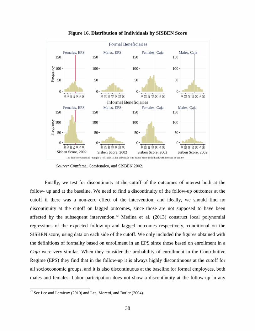
38
Figure 16. Distribution of Individuals by SISBEN Score
Source: Comfama, Comfenalco, and SISBEN 2002.
Finally, we test for discontinuity at the cutoff of the outcomes of interest both at the
follow- up and at the baseline. We need to find a discontinuity of the follow-up outcomes at the
cutoff if there was a non-zero effect of the intervention, and ideally, we should find no
discontinuity at the cutoff on lagged outcomes, since those are not supposed to have been
affected by the subsequent intervention.42 Medina et al. (2013) construct local polynomial
regressions of the expected follow-up and lagged outcomes respectively, conditional on the
SISBEN score, using data on each side of the cutoff. We only included the figures obtained with
the definitions of formality based on enrollment in an EPS since those based on enrollment in a
Caja were very similar. When they consider the probability of enrollment in the Contributive
Regime (EPS) they find that in the follow-up it is always highly discontinuous at the cutoff for
all socioeconomic groups, and it is also discontinuous at the baseline for formal employees, both
males and females. Labor participation does not show a discontinuity at the follow-up in any
42 See Lee and Lemieux (2010) and Lee, Moretti, and Butler (2004).
0
50
100
150Fr
eque
ncy
30 35 40 45 50 55 60
Females, EPS
0
50
100
150
30 35 40 45 50 55 60
Males, EPS
0
50
100
150
30 35 40 45 50 55 60
Females, Caja
0
50
100
150
30 35 40 45 50 55 60
Males, Caja
0
50
100
150
Freq
uenc
y
30 35 40 45 50 55 60
Sisben Score, 2002
Females, EPS
0
50
100
150
30 35 40 45 50 55 60
Sisben Score, 2002
Males, EPS
0
50
100
150
30 35 40 45 50 55 60
Sisben Score, 2002
Females, Caja
0
50
100
150
30 35 40 45 50 55 60
Sisben Score, 2002
Males, Caja
Formal Beneficiaries
Informal Beneficiaries
The data corresponds to "Sample 1" of Table 15, for individuals with Sisben Score in the bandwidth between 30 and 60
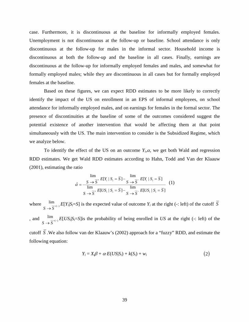
39
case. Furthermore, it is discontinuous at the baseline for informally employed females.
Unemployment is not discontinuous at the follow-up or baseline. School attendance is only
discontinuous at the follow-up for males in the informal sector. Household income is
discontinuous at both the follow-up and the baseline in all cases. Finally, earnings are
discontinuous at the follow-up for informally employed females and males, and somewhat for
formally employed males; while they are discontinuous in all cases but for formally employed
females at the baseline.
Based on these figures, we can expect RDD estimates to be more likely to correctly
identify the impact of the US on enrollment in an EPS of informal employees, on school
attendance for informally employed males, and on earnings for females in the formal sector. The
presence of discontinuities at the baseline of some of the outcomes considered suggest the
potential existence of another intervention that would be affecting them at that point
simultaneously with the US. The main intervention to consider is the Subsidized Regime, which
we analyze below.
To identify the effect of the US on an outcome Yi,α, we get both Wald and regression
RDD estimates. We get Wald RDD estimates according to Hahn, Todd and Van der Klaauw
(2001), estimating the ratio
]|[lim
]|[lim
]|[lim
]|[lim
ˆSSUSE
SSSSUSE
SS
SSYESS
SSYESS
iiii
iiii
=→
−=→
=→
−=→=
−+
−+
α (1)
where )(lim
−+→ SS
E[Yi|Si=S] is the expected value of outcome Yi at the right (-: left) of the cutoff S
, and )(lim
−+→ SS
E[USi|Si=S]is the probability of being enrolled in US at the right (-: left) of the
cutoff S .We also follow van der Klaauw’s (2002) approach for a “fuzzy” RDD, and estimate the
following equation:
Yi = Xiβ + α⋅E(US|Si) + k(Si) + wi
( )2

40
In (2), Yi is again the outcome of interest, Xi is a vector of control variables, USi is a dummy
variable indicating whether individual i was beneficiary of the US, Si is the SISBEN score, and
k(Si) is a polynomial on Si.43
The expected value in (2) is obtained from the following first-stage estimation:
USi = Xiβ + f(Si) + γ⋅1[Si≥ S ] + εi
In (3), f(S) = Σ03ψ0kSk + Σ1
3ψ1k (S- S )k⋅ 1[S≥ S ], where 1[S≥ S ] is an indicator function equal to
one if the term in brackets is true, and zero otherwise. Significance of the γ coefficient
guarantees discontinuity of the probability of enrollment in the US at the cutoff between SISBEN
levels 2 and 3.44 As explained by van der Klaauw (2002), if k(S) and f(S) are correctly specified,
this two-stage procedure leads to consistent estimates of the effect of US, α, on our outcomes.
In addition, provided that X vary smoothly around the cutoff, the TT estimate α̂ would
lead to the same estimate shown in equation (1).
Therefore, if γ≠ 0, the denominator in the foregoing expression is non-zero. This
guarantees an estimable value of α. Finally, it is important to say that the 2002 SISBEN score,
our forcing variable, was estimated that year based on a weighting of variables that led to
discrete values. We follow Lee and Card (2008) to correct for the lack of continuity in that
variable, by estimating equation (2) using robust and clustered (on the individual values of the
SISBEN score) standard errors.45
Notice again that identification also requires that no other factors, different from the
program of interest, cause the discontinuity. As was explained above, enrollment in the
Subsidized Regime also changes discontinuously around the same change in the cutoff
enrollment in the US. If the SR has any impact on the outcomes that are being considered to be
affected by the US, then estimates omitting that effect would be biased, and in that case, it is
important to know the direction of such a bias. Consider a model with two treatments and
assume for the sake of simplicity that individuals are never treated simultaneously for both
43 Specifically, k(S) = Σ1
3βjSj. 44 Note that in this case, some subsamples that were discontinuous in the figures above might not be discontinuous according to equation (1), because this equation is controlling for the polynomial in S and additional variables. 45 See also Lee and Lemieux (2010).
( )3

41
interventions, then our model above would become Yi = Xiβ + αUS⋅E(US|Si) + αSR⋅E(SR|Si) + k(Si)
+ wi. It is straightforward to show that in this case,
α̂ US= [Yi+ - Yi
- -(xSRi+ - xSRi
-) αSR ]/(xUSi+ - xUSi
-) = α̂ - (xSRi+ - xSRi
-) αSR /(xUSi+ - xUSi
-) (4)
where (Yi+ - Yi
-) is equal to the numerator in (1), (xUSi+ - xUSi
-) is its denominator, (xSRi+ - xSRi
-) is
the respective term for the Subsidized Regime, and αSR is the impact of the Subsidized Regime
on Yi. In other words, by using RDD to estimate αUS in the presence of other intervention like the
SR, according to (4) we would be overestimating (underestimating) αUS if αSR is positive
(negative), in a magnitude equal to the second term in the right-hand side of equation (4).
By 2005, in Medellin there were more than 150,000 beneficiaries of the Subsidized
Regime, but only about 7,000 beneficaries of the Unemployment Subsidy. That is, beneficiaries
of the US were nearly 4.5 percent of the beneficiaries of the Subsidized Regime. Since the
number of beneficiaries of the US is small relative to the number of beneficiaries of the SR, we
can drop the beneficiaries of the US from our data and use equation (2) with the rest of the data
to get an unbiased estimate of (Yi+ - Yi
-) and (xSRi+ - xSRi
-) within that population, to estimate the
impact of the SR on our outcomes of interest. We present those results below.
In the following two subsections, we present RDD estimates of the effect of the
unemployment subsidy on a subset of outcomes, focusing on individuals between 20 to 55 years
of age.
5. Results Table 4 presents the effects of the US on our set of outcomes based on the Wald and Regression
RDD estimates defined in equations (1) and (2). There are five panels in the table, one for each
outcome: Labor Force Participation, Unemployment, School Attendance, Household Income,
and Earnings; and eight columns, one for each population considered: four for females and four
for males. For each gender we have two panels for formal employees, one based on their
enrollment at the baseline in an EPS (Contributive Regime) and the other based on their
enrollment in a Caja. The other two panels per gender are for informal employees based on the
same two concepts, EPS and Caja. For each outcome, we obtained Wald estimates using

42
bandwidths of 2, 4, and 8 points of the SISBEN score, and for each bandwidth, we report the
estimated numerator and denominator of equation (1), and its corresponding ratio, which is the
parameter of interest. For the regression estimates, the bandwidths used in the regression were of
20 points without control variables (row A), 20 with control variables (row B) and 30 with
control variables (row C).
The shadow areas of our Wald estimates are those in which we did not find evidence of
discontinuity, that is, where the coefficient of the denominator was not statistically different from
zero. The blank areas in our regression estimates are those in which we did not find evidence of a
discontinuity using the regression estimates of equation (2), that is, when the γ coefficient was
not statistically different from zero.
According to our Wald estimates, no ratio between the numerators and denominator is
statistically different from zero, and thus, there is no effect of the US on the assessed outcomes
for any of the populations.
When we focus on or regression RDD estimates, we omit the results for males in the
informal sector since we did not find the required discontinuity at the cutoff for that group.
Evidence of the discontinuities is presented in the last three rows of the table, where we present,
for each bandwidth considered (A, B or C), the estimated γ coefficients. Row A only includes as
control variables in equations (2) and (3) the polynomials in S, k(S), and f(S), and individuals
within a “bandwidth” of 20 SISBEN points, 10 on each side of the cutoff; row B uses the same
bandwidth, and in addition to the polynomials in S, it also includes a set of control variables
whose descriptive statistics are presented in Medina et al. (2013). Finally, row C also includes
the polynomials in S and the control variables from row B, but in that case it includes individuals
with SISBEN scores in the interval 30 <S< 60. The sample considered consisted of individuals
whose outcome was observed within two years of receiving the US.46
Since in the population studied the subset of beneficiaries at t1 who are enrolled in an EPS
and also belong to SISBEN levels 1 or 2 is negligible, we are unable to use RDD to identify the
effect of the US on EPS enrollment.
Overall, the only regression RDD results included are those in which we found a
discontinuity, with at least 5 percent of significance. We find a significant discontinuity for 46 Similar results were obtained when we considered individuals whose baseline survey also occurred within two years prior to enrollment in the US.

43
females employed in the formal and informal sectors. For males, we only find discontinuity for
formally employed workers. Our estimates consistently imply a negative impact of the US
participation on the earning of beneficiaries and a somewhat weaker negative impact on
household earnings. Although the results show a strong and robust reduction of earnings of
female and male beneficiaries, the magnitude of the estimated coefficients seems too large. The
baseline earnings of female beneficiaries vary between $50,000 and $90,000 Colombian pesos,
while those of male beneficiaries vary between $90,000 and $150,000 Colombian pesos (see
Medina et al., 2013). The negative effect nonetheless can be partly explained by the so-called
earnings dip pointed out by Ashenfelter (1978) and by Heckman and Smith (1999). Specifically,
if individuals experienced a drop in earnings before applying to the program, it would be very
difficult to find a comparison group able to resemble the earnings pattern of the hypothetical
ideal control group. Since individuals in the treated group in this program are required to have
experienced unemployment, their earnings before entering are very likely to have dropped. Thus,
if their baseline earnings are measured relatively before the drop takes place, and the follow-up is
measured when the earnings have not recuperated their former level, then the estimated effect is
very likely to be underestimated if we are not able to simulate a comparison group that would
experience a similar earnings pattern. In the next section we perform a matching differences-in-
differences estimation with a similar sample of individuals we are using here, but also, with a
sample that only considers individuals who were unemployed at the baseline.
We find no effect on labor participation or unemployment. Once we use a larger
bandwidth, as we do in panel C of the Tables, the discontinuity becomes significant in a greater
number of cases. The larger the bandwidth, nonetheless, the more important it is for our
polynomial k(S) and f(S) to be correctly specified.
Finally, the table shows a positive effect on formally employed females’ school
attendance and a positive on formally employed males’ attendance. There is also a positive effect
in the case of informally employed females, although those coefficients are very large.
Altogether, the results reveal some limitations in the power of the regression RDD to
correctly identify the impact of the intervention. We tried several other specifications, most of
them leading to similar results in terms of signs and magnitude of the coefficients. The different
specification included variations in the polynomials in the SISBEN score and its piecewise
components. We also obtained estimations with the outcomes in differences (follow-up minus

44
baseline), and in levels controlling for all the baseline outcomes. None of those led us to obtain
reasonable magnitudes in all household income and earnings coefficients.47 In addition, we used
another definition of formality according to which individuals were classified as formal if they
were employees at the baseline. We only found discontinuity for the population of females
employed in the informal sector, with no effect in any outcome but household income and
earnings, which were again too large.
5.1 Regression RDD Estimates of the Effect of the Subsidized Regime Regarding the possibility that the impact of the Subsidized Regime would be limiting the
possibility for us to obtain unbiased estimates of the effect of the US, we obtained RDD
estimates of the impact of the SR on our set of outcomes (see Medina et al., 2013). The results
are very consistent across samples, bandwidths, the inclusion of control variables, and the
definition of formality. Overall, we find a robust discontinuity at the cutoff of the probability of
being enrolled in the SR. In addition, the magnitudes of most coefficients seem very reasonable
when compared with those found when estimating the effect of the US.
Importantly, there is no positive effect of the SR on household income or earnings, which
means that the negative effects of the US on those variables would not be explained by the effect
of the SR, because the effect of the SR, if any, would overestimate our estimate of the impact of
the US. This implies that there would be reasons other than the concurrence of another
intervention at the cutoff that should be explaining the huge negative US effects we estimated.
Lack of consistency across specifications and in some cases, across definitions of formality, plus
the limitations posed by the discontinuities of the lagged outcomes we found, might be among
the causes of that result.
47 We also obtained estimates for the sample of heads of household (not included here) similar to the ones included in Table 4.

45
Table 4. Wald and Regression RDD Estimates of the Unemployment Subsidy
Coeff. z Coeff. z Coeff. z Coeff. z Coeff. z Coeff. z Coeff. z Coeff. zBandwidth Variable
numer 0.051 1.61 0.045 * 1.66 -0.011 -1.61 -0.012 * -1.84 -0.010 -0.36 -0.010 -0.38 -0.007 -1.09 -0.007 -1.00denom 0.038 ** 2.34 0.056 ** 3.04 0.007 ** 3.98 0.002 1.37 0.042 1.64 0.069 ** 2.35 0.001 0.54 0.003 ** 2.24lwald 1.346 0.11 0.817 1.12 -1.502 -1.17 -5.024 -0.41 -0.225 -0.04 -0.141 -0.12 -10.488 -0.02 -2.526 -0.31numer 0.046 1.25 0.039 1.13 -0.010 -1.12 -0.010 -1.06 0.012 0.34 0.010 0.32 -0.011 -1.32 -0.012 -1.33denom 0.028 * 1.70 0.022 1.02 0.006 ** 2.21 0.001 0.47 0.031 1.05 0.056 1.62 0.000 0.24 0.004 ** 2.53lwald 1.649 0.62 1.764 0.14 -1.686 -0.21 -8.756 -0.25 0.382 0.12 0.174 0.07 -33.094 -0.53 -3.019 -0.57numer 0.026 1.18 0.019 0.86 -0.004 -0.58 -0.004 -0.57 0.001 0.04 0.004 0.20 -0.006 -1.18 -0.006 -0.99denom 0.031 ** 2.72 0.046 ** 3.63 0.004 ** 2.71 0.001 0.97 0.045 ** 2.24 0.070 ** 3.84 0.000 0.38 0.003 ** 3.35lwald 0.846 0.99 0.419 0.74 -0.869 -0.30 -2.427 -0.09 0.021 0.01 0.058 0.17 -15.011 -0.07 -1.912 -0.77
20 A 0.571 1.03 -0.309 -0.24 -0.332 -0.19 0.106 0.44 0.047 0.2520 B -0.482 -0.38 -0.471 -0.28 0.258 0.95 0.126 0.5830 C -0.283 -0.96 -0.180 -1.33 -0.016 -0.01 0.183 0.11 -0.041 -0.28 -0.036 -0.31
numer 0.002 0.20 -0.003 -0.39 0.000 -0.14 0.000 0.00 0.010 0.44 0.018 1.03 -0.008 * -1.65 -0.008 -1.27denom 0.038 ** 2.67 0.056 ** 3.60 0.007 ** 3.89 0.002 1.27 0.042 1.61 0.069 ** 3.16 0.001 0.60 0.003 ** 2.21lwald 0.044 0.17 -0.058 -0.31 -0.060 -0.11 -0.001 0.00 0.242 0.20 0.267 0.86 -13.049 -0.17 -2.932 -0.73numer -0.001 -0.15 -0.006 -0.59 0.001 0.14 0.001 0.29 0.005 0.19 0.010 0.51 -0.002 -0.26 -0.002 -0.25denom 0.028 * 1.67 0.022 1.24 0.006 ** 2.59 0.001 0.54 0.031 1.00 0.056 ** 1.97 0.000 0.23 0.004 ** 2.39lwald -0.053 -0.03 -0.292 -0.05 0.113 0.06 0.963 0.01 0.169 0.02 0.182 0.29 -5.145 -0.21 -0.528 -0.04numer 0.007 1.07 0.003 0.41 0.001 0.48 0.002 0.65 0.001 0.07 0.008 0.51 0.000 -0.11 0.000 -0.05denom 0.031 ** 2.79 0.046 ** 3.63 0.004 ** 2.48 0.001 1.07 0.045 ** 2.30 0.070 ** 4.23 0.000 0.45 0.003 ** 2.57lwald 0.214 0.88 0.056 0.35 0.328 0.33 1.226 0.03 0.031 0.02 0.107 0.47 -1.209 -0.04 -0.091 -0.04
20 A -0.031 -0.19 0.177 0.34 0.196 0.27 -0.088 -0.49 -0.058 -0.4020 B 0.003 0.01 -0.019 -0.03 -0.169 -0.78 -0.142 -0.7930 C -0.087 -0.91 -0.023 -0.50 0.594 1.23 0.872 1.19 -0.014 -0.12 0.017 0.18
numer -0.005 -0.59 -0.007 -0.88 -0.002 -0.61 -0.002 -0.89 0.006 0.68 0.006 0.59 0.002 1.18 0.002 0.93denom 0.038 ** 2.72 0.056 ** 2.85 0.007 ** 4.42 0.002 1.54 0.042 * 1.75 0.069 ** 3.46 0.001 0.54 0.003 * 1.91lwald -0.124 -0.43 -0.127 -0.27 -0.233 -0.48 -0.770 -0.07 0.131 0.22 0.086 0.53 3.827 0.08 0.820 0.08numer -0.004 -0.50 -0.005 -0.60 -0.002 -0.69 -0.002 -0.89 0.003 0.29 0.003 0.27 0.001 0.33 0.001 0.27denom 0.028 * 1.83 0.022 0.94 0.006 ** 2.76 0.001 0.64 0.031 1.09 0.056 ** 2.53 0.000 0.22 0.004 ** 2.08lwald -0.157 -0.15 -0.247 -0.02 -0.415 -0.15 -2.088 -0.13 0.103 0.09 0.058 0.16 2.979 0.16 0.250 0.00numer -0.006 -0.86 -0.008 -1.15 -0.004 * -1.68 -0.004 ** -2.01 0.004 0.48 0.004 0.53 0.002 0.73 0.001 0.66denom 0.031 ** 2.84 0.046 ** 3.25 0.004 ** 3.45 0.001 1.09 0.045 ** 2.28 0.070 ** 4.86 0.000 0.35 0.003 ** 2.47lwald -0.190 -0.36 -0.164 -0.86 -0.882 -0.84 -2.609 -0.16 0.079 0.14 0.060 0.54 3.967 0.20 0.507 0.10
20 A 0.200 1.15 0.837 ** 2.51 1.072 ** 2.32 -0.141 * -1.91 -0.110 * -220 B 0.801 ** 2.34 1.000 ** 2.17 -0.190 ** -2.09 -0.156 ** -230 C 0.094 0.99 0.088 ** 2.01 0.978 ** 3.16 1.400 ** 2.96 -0.117 ** -2.15 -0.097 ** -2
RegressionEstimates
RegressionEstimates
School Attendance
WaldEstimates
2
4
8
RegressionEstimates
Unemployment
WaldEstimates
2
4
8
(vii) EPS (viii) Caja
Labor Force Participation
WaldEstimates
2
4
8
(i) EPS (ii) Caja (iii) EPS (iv) Caja (v) EPS (vi) Caja
Females MalesFormal Informal Formal Informal

46
Table 4. Wald and Regression RDD estimates of the Unemployment Subsidy (Continuation)
Coeff. p z Coeff. p z Coeff. p z Coeff. p z Coeff. p z Coeff. p z Coeff. p z Coeff. p z
numer -2884 -0.18 -3322 -0.21 -14047 ** -3.09 -13867 ** -4.04 20836 1.06 16598 1.01 -9612 ## -2.09 -9812 ** -2.13denom 0.038 ** 2.96 0.056 ** 2.74 0.007 ** 3.49 0.002 * 1.70 0.042 * 1.90 0.069 ** 3.12 0.001 ## 0.52 0.003 * 1.92lwald -75454 -0.11 -59822 -0.16 -1940903 -1.12 -5990592 -0.61 490359 0.06 241144 0.78 -15000000 ## -0.01 -3419492 -0.91numer 11634 0.54 16495 0.80 -7670 -1.33 -7736 -1.56 24893 1.06 22946 1.35 2355 ## 0.37 1939 0.29denom 0.028 ** 2.11 0.022 0.99 0.006 ** 2.53 0.001 0.68 0.031 0.99 0.056 ** 2.22 0.000 ## 0.20 0.004 * 1.95lwald 418689 0.01 749210 0.04 -1335728 -0.15 -6743727 -0.65 813690 0.10 408495 0.31 7058207 ## 0.15 507587 0.07numer -4315 -0.34 -1841 -0.16 1663 0.41 1571 0.50 -4488 -0.26 -8523 -0.57 6511 ## 1.57 6183 1.54denom 0.031 ** 3.09 0.046 ** 2.95 0.004 ** 2.70 0.001 1.13 0.045 ** 3.19 0.070 ** 4.50 0.000 ## 0.41 0.003 ** 2.30lwald -140608 -0.26 -39979 -0.14 393444 0.21 1062414 0.20 -99451 -0.23 -121043 -0.52 17000000 ## 0.29 2104759 0.30
20 A -921667 ** -3.31 -476353 -0.87 -601611 -0.80 -110160 -0.84 -147548 -120 B -925932 * -1.86 -1215877 * -1.81 -12031 -0.08 -83193 -0.6830 C -281212 ** -2 -159239 ** -2.53 -621705 -1.39 -893254 -1.31 -83372 -0.98 -100583 -2
numer 8305 1.04 5634 0.84 -4743 * -1.94 -4880 ** -2.55 -12743 -0.94 -17288 -1.40 -4423 ## -1.59 -4558 -1.25denom 0.038 ** 2.75 0.056 ** 3.25 0.007 ** 4.05 0.002 * 1.72 0.042 * 1.76 0.069 ** 2.93 0.001 ## 0.58 0.003 ** 2.08lwald 217306 0.10 101453 0.53 -655390 -1.24 -2108061 -0.05 -299884 -0.28 -251167 -0.59 -6908176 ## -0.36 -1588358 -0.30numer 14847 * 1.65 12066 1.40 -2744 -0.83 -2832 -1.08 -3488 -0.20 -6985 -0.44 -3992 ## -1.14 -4103 -0.84denom 0.028 * 1.67 0.022 1.07 0.006 ** 2.73 0.001 0.74 0.031 1.16 0.056 ** 2.00 0.000 ## 0.22 0.004 ** 2.13lwald 534356 0.22 548074 0.17 -477781 -0.35 -2468545 -0.34 -114008 -0.06 -124347 -0.16 -12000000 ## -0.55 -1074003 -0.15numer -461 -0.08 -2377 -0.39 -2447 -1.16 -2524 -1.63 -11388 -1.02 -14821 * -1.67 -3166 ## -1.27 -3215 -1.16denom 0.031 ** 2.54 0.046 ** 3.68 0.004 ** 3.02 0.001 1.23 0.045 ** 2.29 0.070 ** 4.14 0.000 ## 0.38 0.003 ** 2.72lwald -15024 -0.05 -51629 -0.33 -579127 -0.92 -1707110 -0.36 -252335 -0.22 -210481 -0.95 -8256146 ## -0.38 -1094375 -0.64
20 A -125002 -0.71 -697681 ** -2.04 -941398 ** -1.99 -697681 ** -2.04 -941398 ** -220 B -686736 ** -2.03 -888819 * -1.95 -96313 -0.76 -124977 -130 C -203125 ** -2 -130312 ** -2.96 -534156 * -1.75 -772516 * -1.66 -152577 ** -2.20 -141594 ** -3
A 1[S<Ŝ], γ 0.030 ** 2.34 0.004 ** 3.30 0.003 ** 3.78 0.068 ** 4.30 0.084 ** 5B 1[S<Ŝ], γ 0.004 ** 3.22 0.003 ** 3.77 0.055 ** 3.77 0.067 ** 4C 1[S<Ŝ], γ 0.045 ** 5 0.094 ** 9.32 0.004 ** 3.77 0.003 ** 3.99 0.084 ** 6.70 0.108 ** 8
RegressionEstimates
1st Stage
RegressionEstimates
A. Only Polynomial term in S, Bandwidth: 20 (38 < S < 57); B. Polynomial term in S and Control Variables, Bandwidth: 20 (38 < S < 57); C. Polynomial term in S and Control Variables, Bandwidth: 30 (30 < S < 60)The average exchange rate between 2005 and 2006 was $2,340/USD.
RegressionEstimates
Earnings
WaldEstimates
2
4
8
(vii) EPS (viii) Caja
Household Income
WaldEstimates
2
4
8
(i) EPS (ii) Caja (iii) EPS (iv) Caja (v) EPS (vi) Caja
Females MalesFormal Informal Formal Informal

47
5.2 RDD: Synthesis We obtained both Wald and Regression RDD estimates of the impact of the US on a battery of
outcomes. We also present evidence that supports the identifying assumptions underlying RDD.
According to our Wald estimates, the US program had no significant effect on any of the
outcomes considered, while our regression RDD estimates do point to a negative effect on
earnings and household income, and a positive effect on school attendance of females. There
were nonetheless some facts that prevent us from considering the regression RDD estimates
robust enough.
We now proceed to complement these results with matching estimates, which as we will
see, will lead us to estimates of much more reasonable magnitudes, in particular, on variables
like household income and earnings.
5.3 Matching Estimators
Since the RDD strategy only allows us to identify program impacts near the cutoff S , it can be
useful to complement those estimates with additional ones that could give us mean impacts for a
broader population of US participants. We now obtain them by using the matching method.
This method assumes that selection into the program is based on the observed variables in
the data set. The crux of this approach is that treatments and controls with the same observed
characteristics are assumed to be allocated randomly between program and non-program status.
Even though the sample of beneficiaries seems very different to that of non-beneficiaries, that
should not pose significant limits to applying the matching estimators, since there is a large set of
people in the comparison group from which to get the matches for each beneficiary in the
treatment group. Medina et al. (2013) include descriptive statistics of the variables on which the
matching was performed between beneficiaries and non-beneficiaries of the US (treated and
comparison group). Prior to matching, the mean differences between these groups’
characteristics are in most cases statistically significant. After matching, these mean differences
are negligible and never statistically significant. Similar results follow for the other subsamples.
We obtain matching differences-in-differences and cross-section estimates for all
outcomes of interest, except for those outcomes for which we only have information at the
follow-up survey, such as unemployment duration, or “enrolled in an EPS.” For these variables
we can only obtain cross-section estimates.
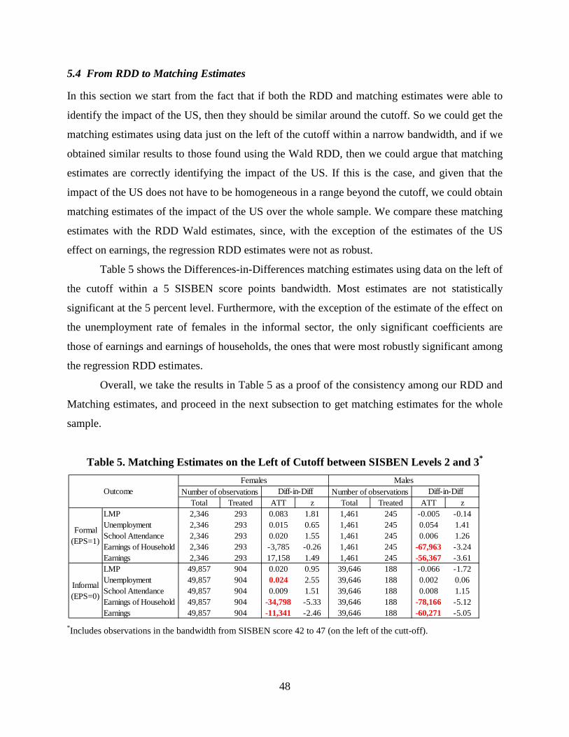
48
5.4 From RDD to Matching Estimates In this section we start from the fact that if both the RDD and matching estimates were able to
identify the impact of the US, then they should be similar around the cutoff. So we could get the
matching estimates using data just on the left of the cutoff within a narrow bandwidth, and if we
obtained similar results to those found using the Wald RDD, then we could argue that matching
estimates are correctly identifying the impact of the US. If this is the case, and given that the
impact of the US does not have to be homogeneous in a range beyond the cutoff, we could obtain
matching estimates of the impact of the US over the whole sample. We compare these matching
estimates with the RDD Wald estimates, since, with the exception of the estimates of the US
effect on earnings, the regression RDD estimates were not as robust.
Table 5 shows the Differences-in-Differences matching estimates using data on the left of
the cutoff within a 5 SISBEN score points bandwidth. Most estimates are not statistically
significant at the 5 percent level. Furthermore, with the exception of the estimate of the effect on
the unemployment rate of females in the informal sector, the only significant coefficients are
those of earnings and earnings of households, the ones that were most robustly significant among
the regression RDD estimates.
Overall, we take the results in Table 5 as a proof of the consistency among our RDD and
Matching estimates, and proceed in the next subsection to get matching estimates for the whole
sample.
Table 5. Matching Estimates on the Left of Cutoff between SISBEN Levels 2 and 3*
*Includes observations in the bandwidth from SISBEN score 42 to 47 (on the left of the cutt-off).
Total Treated ATT z Total Treated ATT zLMP 2,346 293 0.083 1.81 1,461 245 -0.005 -0.14Unemployment 2,346 293 0.015 0.65 1,461 245 0.054 1.41School Attendance 2,346 293 0.020 1.55 1,461 245 0.006 1.26Earnings of Household 2,346 293 -3,785 -0.26 1,461 245 -67,963 -3.24Earnings 2,346 293 17,158 1.49 1,461 245 -56,367 -3.61LMP 49,857 904 0.020 0.95 39,646 188 -0.066 -1.72Unemployment 49,857 904 0.024 2.55 39,646 188 0.002 0.06School Attendance 49,857 904 0.009 1.51 39,646 188 0.008 1.15Earnings of Household 49,857 904 -34,798 -5.33 39,646 188 -78,166 -5.12Earnings 49,857 904 -11,341 -2.46 39,646 188 -60,271 -5.05
Informal(EPS=0)
OutcomeFemales
Diff-in-DiffNumber of observations Number of observationsMales
Diff-in-Diff
Formal(EPS=1)

49
5.5 Matching Estimates Results are disaggregated by gender, formality status, and for the periods between 2002 and 2005
and between 2005 and 2009. For all of these cases we estimate the effect on the seven outcomes
mentioned above. We could not present RDD estimates for the 2005 to 2009 period due to lack
of sufficient evidence of a discontinuity in enrollment.
5.6 Labor Market Outcomes Table 6 presents all of our matching estimators. The columns are divided by gender, and within
each gender we include columns for formal and informal workers between 21 and 54 years of
age, according to enrollment in an EPS or a Caja. The rows include the estimated coefficients for
each time period considered, namely, 2002 to 2005 and 2005 to 2009. Within each period we
include results for all workers, and also for workers who were heads of household at the baseline.
Within each population we include both cross-section and differences-in-differences estimates of
the impact of the US on labor market participation, unemployment, enrollment in an EPS,
earnings of the household, and earnings of the worker.48 The table also presents estimates
obtained when beneficiaries are split according to the type of training courses they took while in
the US program, namely those related to industrial affairs, management and services, technology
and software, and other courses.
Here we describe our DID estimates obtained for the period between 2005 and 2009, the
period in which the sample included the largest number of US beneficiaries. For women in the
formal sector, US participation led to a slight decline in labor force participation when formality
is measured by previous enrollment in a Caja (0.0 to 3.7 percent), and a larger one when
measured by previous enrollment in an EPS (7.8 to 8.5 percent), had no effect on unemployment,
and caused a fall in both individual and household earnings.
DID-matching estimates are much smaller and more reasonable than those found with
RDD. Among women in the formal sector, the estimated impacts of the US are very large
relative to the treatment group baseline earnings reported in Medina et al. (2013), accounting for
a reduction of earnings between 18 and 49 percent ($21,993 and $82,387, respectively). The
magnitude of the impact is partly explained by the beneficiaries’ low earnings at baseline. In 48 See Medina et al. (2013) for a summary of the variables employed in the estimations presented in this section, for the period between 2002 and 2005, and between 2005 and 2009.

50
fact, the magnitude of these impacts is small when compared with the monthly minimum wage,
with respect to which the effect is between 4 and 17 percent.
Among women in the informal sector, US participation had no effect on labor force
participation and led to a slight increase in unemployment. In addition, both individual and
household earnings fell, but this earnings decline was smaller than the earnings declines
experienced by women in the formal sector. In this case, the decline in earnings is between 22
and 27 percent of baseline earnings ($26,687 and $25,583), but only 5 percent of the monthly
minimum wage.
Our DID estimates indicate that the impact of the US on labor market outcomes also
varied by participation in training. For women in the formal sector, labor force participation fell
regardless of the type of training they took while they were US beneficiaries. This estimated
decline was larger than the estimated declines found when females were not split by the type of
training courses they took.
Unemployment fell for formal sector females who took courses in industrial affairs and
other topics, while it remained unchanged for those who took courses in management and
services and in technology and software. Both individual and household earnings fell, although
by a smaller amount for formal sector females who took courses in technology and software.
Among informal sector females, the US program did not appear to affect labor force
participation, and there was a slight increase in unemployment (1.2 percent). Although
unemployment duration increased and individual earnings fell for these women, for females who
took courses in technology and software topics, household earnings fell, whereas they remained
unchanged for women in the informal sector who took courses in management and services.
Among males from the formal sector, we found that US participation causes labor force
participation to fall by more than it fell for informally employed females (between 5.7 and 9.9
percent). Unemployment increases for the subsample of male heads of household (4.3 to 5.5
percent), while it remains unchanged for the entire sample of males. Both individual and
household earnings fall. Informally employed males also reduce their labor force participation,
but by half as much as for formally employed males. Their unemployment rates are unaffected,
although their unemployment duration increases. Finally, and as is true for females, the decrease
in earnings is larger among formal compared to males in the informal sector. This decline in
earnings of males in the formal sector is between 34 and 61 percent of their baseline earnings

51
($74,985 and $138,733) and between 15 and 28 percent of the monthly minimum wage. Among
males in the informal sector, the decline is between 18 and 22 percent of their baseline earnings
($40,287 and $46,030) and between 8 and 9 percent of the minimum wage.
Labor force participation of males in the formal sector falls regardless of the types of
training they took, although the reduction is smaller for those who took courses in technology
and software. Unemployment of males in the formal sector is not affected by the types of
training courses they took. Individual earnings fall regardless of the type of training they took,
but household earnings fall for all types of training, except for management and services courses.
The results included in the table for informally employed males are not robust due to the small
size of the sample of beneficiaries.
5.7 Human Capital and Nutrition Outcomes An important function of unemployment insurance is that it helps individuals and their families
to “smooth” their consumption, particularly their human capital investment, when they are
unemployed and their earnings are low. Our data contain no information on household
consumption, but they include several other related variables, such as participants’ school
attendance, the school attendance rate of all household members 6 to 18 years old, weight,
height, body mass index (BMI), and the Apgar score of the female beneficiaries’ children at
birth.49 These variables are all imperfect indicators of smoothing consumption, since the US may
prevent household members from dropping out of school, and it may help pregnant women to
maintain minimum nutrition standards. BMI may take many months to influence. However,
looking at these variables collectively may provide indirect evidence on whether the US program
is achieving its key objective: to smooth human capital investment and nutrition of Colombia’s
poorest (urban) families when they become unemployed.
School attendance among females employed in the formal and informal sectors increases
with the US for the whole sample of females, although on a small scale (1.0 percent). The school
49 The BMI is the ratio of the children’s weight to the square of their height, expressed in kilograms per square meter. The Apgar score is only available in the 2006 and 2007 surveys, and it is determined by evaluating the newborn on five simple criteria on a scale from zero to two, then summing up the five values obtained. The resulting Apgar ranges from zero to 10. The five criteria are appearance, pulse, grimace, activity, and respiration. Apgar1 and Apgar5 refer to the same concept assessed after 1 and 5 minutes after the child’s birth. We defined each Apgar as 1 if the score was 7 or more, and zero otherwise. See descriptive statistics in Medina et al. (2013), where beneficiaries’ socioeconomic variables suggest they are worse off than non-beneficiaries.

52
index is not affected by the US except for informally employed females, where it is negative.
The US has no effect on these outcomes for female heads of household. Although the results
based on the 2005 to 2009 data imply negative effects of the US on weight and height at birth,
after controlling for the education of the mother and the father (available only for 2006 and
2007), no effect of the US is found on weight, height, or BMI at birth of beneficiaries’ children.
The US has a positive effect on school attendance of formally and informally employed
males of around 2.0 percent, but it has no effect on heads of household. On the contrary, it has a
negative effect on the school index, especially of informal workers. These results suggest that
individuals who were not heads of household at the baseline in 2005, who are presumably
relatively younger and with smaller family sizes than those who were already heads of household
by then, face liquidity constraints that prevent them from attending school. In addition, the fact
that such a small economic benefit makes a difference that allows them to attend school is an
indication of their precarious economic condition. This result is consistent with that found for
Indonesia by Chetty and Looney (2006), and with evidence showing the effects of US benefits
on smoothing consumption by Gruber (1997, 1998), Browning and Crossley (2001), and
Bloemen and Stancanelli (2005).
5.8 Matching DiD Estimators using only the Unemployed at Baseline Although we consider our matching estimates are reasonable, it is not easy for the method to
correctly resemble all the characteristics and facts of the treated population with the universe of
individuals in the comparison group. Specifically, in theory, we know that at baseline, all treated
individuals are supposed to suffer a shock that would lead them to apply for the US, while it is
not possible to know who among the comparison group will suffer a comparable shock, and
information used to match people from both groups seems limited to predict the likelihood of
such events.
To assess whether not having information for the comparison group about whether people
in that group suffered a shock in the analyzed period, we obtain matching differences-in-
differences estimates for the sample of all individuals who were unemployed at the baseline, and
for the sample of all individuals in the treatment group (regardless of their employment status at
the baseline) and the subset of individuals in the comparison group who were unemployed at the
baseline. By including individuals in the comparison group who were unemployed at the

53
baseline, we ensure that at least at that moment they suffered an employment shock; thus, we
would expect that those estimates would not underestimate the impacts, but rather, they might
actually provide an upper bound of them.
When we compare the estimates obtained for females in Table 6 with the results obtained
for the subsample of individuals who were unemployed at the baseline (Medina et al., 2013), we
find that the effect on household income becomes non-significant for the sample of individuals
who were unemployed at the baseline. A similar result is found for formally employed females,
although the effect of the US on informally employed females becomes more negative. In the
sample of formally employed females, other estimates become much larger, as is the case for the
impact on labor participation and unemployment, particularly when we consider the sample of all
formally employed females. The sample of unemployed female heads of household at the
baseline becomes too small.
When the results obtained for males in Table 6 are compared with those obtained for the
subsample of individuals who were unemployed at the baseline (Medina et al., 2013), only the
effects on earnings become of similar magnitude and significance, while all other estimates
become non-significant, presumably because of the smaller number of available observations.
In short, when we use the sample of unemployed individuals at the baseline, the effects of
the US on household income and earnings become much less negative, or in the worst case, of
similar magnitude as those obtained when we used all individuals available at the baseline. For
females, we found larger effects on labor participation and unemployment, while those become
negligible for males.

54
Table 6. Matching Estimators: Whole Sample and Heads of Household.
Training Sample Method Coeff. z Coeff. z Coeff. z Coeff. z Coeff. z Coeff. z Coeff. z Coeff. z
All CS -0.063 ** -3.08 -0.074 ** -4.91 0.014 1.16 0.022 ** 2.28 -0.096 ** -5.73 -0.094 ** -6.25 -0.070 ** -4.09 -0.067 ** -3.25DiD 0.004 0.21 0.001 0.07 0.007 0.66 -0.009 -0.65 -0.080 ** -4.53 -0.081 ** -5.16 -0.064 ** -3.46 -0.056 ** -2.48
HH DiD -0.018 -0.72 -0.044 ** -2.21 -0.011 -0.88 -0.017 -1.07 -0.087 ** -4.70 -0.086 ** -5.07 -0.085 ** -4.72 -0.076 ** -3.51All CS -0.005 -0.46 -0.016 * -1.88 0.029 ** 3.43 -0.102 ** -9.87 -0.086 ** -9.43 -0.011 -0.72
DiD -0.085 ** -6.56 -0.003 -0.34 -0.010 -1.02 -0.078 ** -6.83 -0.057 ** -5.77 -0.045 ** -2.55HH DiD -0.018 -0.72 -0.044 ** -2.21 -0.011 -0.88 -0.017 -1.07 -0.087 ** -4.7 -0.086 ** -5.07
Not Defined All CS -0.128 ** -6.98 -0.049 ** -3.67 -0.043 ** -2.50 -0.127 ** -6.12 -0.115 ** -6.12 -0.116 ** -2.71Industrial All CS -0.125 ** -5.90 -0.023 -1.54 0.001 0.07 -0.110 ** -4.37 -0.095 ** -4.28 -0.092 * -1.89Manag & Serv All CS -0.152 ** -6.13 -0.089 ** -4.50 -0.055 * -1.72 -0.109 ** -3.29 -0.101 ** -3.21 -0.247 ** -2.53Tech & Soft All CS -0.116 ** -3.67 -0.038 -1.45 -0.031 -0.76 -0.053 -1.55 -0.067 ** -2.15 -0.269 ** -3.42
All CS 0.030 ** 3.35 0.023 ** 3.89 0.011 ** 2.12 0.002 0.57 0.102 ** 6.62 0.109 ** 7.94 0.052 ** 3.44 0.034 * 1.92DiD -0.037 ** -2.8 0.001 0.07 0.002 0.32 0.011 1.35 -0.009 -0.42 0.007 0.36 0.040 ** 1.99 0.022 0.95
HH DiD -0.032 * -1.76 -0.036 ** -2.75 0.001 0.14 0.002 0.22 0.040 * 1.90 0.050 ** 2.57 0.024 1.19 0.007 0.28All CS 0.049 ** 9.95 0.035 ** 10.65 0.006 ** 1.99 0.088 ** 10.1 0.080 ** 10.6 -0.003 -0.21
DiD -0.009 -1.44 -0.013 ** -2.97 0.012 ** 2.48 0.008 0.76 0.001 0.14 0.024 1.344HH DiD -0.032 * -1.76 -0.036 ** -2.75 0.001 0.14 0.002 0.22 0.040 * 1.9 0.050 ** 2.57
Not Defined All CS -0.023 ** -2.52 -0.021 ** -3.29 0.003 0.29 0.045 ** 2.50 0.024 1.48 -0.038 -0.97Industrial All CS -0.047 ** -4.53 -0.021 ** -3.13 0.025 ** 2.85 0.001 0.02 -0.013 -0.61 -0.047 -0.92Manag & Serv All CS -0.009 -0.72 -0.017 * -1.68 -0.011 -0.62 0.008 0.24 0.013 0.43 0.024 0.26Tech & Soft All CS -0.022 -1.32 -0.008 -0.59 0.000 0.00 0.034 1.31 0.000 0.01 -0.063 -0.83
All CS -0.001 -0.14 -0.004 -0.98 0.0004 0.14 -0.006 -1.59 0.002 0.41 0.004 0.89 -0.001 -0.29 0.002 0.27DiD 0.017 * 1.8 0.010 * 1.66 0.004 1.24 -0.001 -0.29 0.009 1.22 0.008 1.24 0.001 0.19 0.002 0.26
HH DiD 0.010 0.88 0.002 0.23 0.000 -0.05 -0.013 ** -2.21 -0.002 -0.32 0.000 -0.07 -0.007 -1.34 -0.005 -0.94All CS 0.006 1.53 0.007 ** 2.8 0.009 ** 3.9 0.007 * 1.83 0.008 ** 2.23 0.010 * 1.85
DiD 0.011 ** 2.11 0.009 ** 2.54 0.016 ** 4.92 0.019 ** 3.25 0.018 ** 3.51 0.022 ** 2.84HH DiD 0.010 0.88 0.002 0.23 0.000 -0.05 -0.013 ** -2.21 -0.002 -0.32 0.000 -0.07
Not Defined All CS -0.030 ** -2.05 -0.003 -0.33 0.008 1.58 -0.028 ** -2.53 -0.023 ** -2.29 -0.006 -0.38Industrial All CS -0.004 -0.32 0.004 0.49 0.006 1.02 -0.014 -1.23 -0.011 -1.03 -0.013 -0.70Manag & Serv All CS -0.060 ** -2.83 -0.033 ** -2.36 -0.003 -0.28 -0.039 * -1.73 -0.036 * -1.73 0.002 0.22Tech & Soft All CS 0.034 ** 2.44 0.016 1.27 0.008 0.41 0.006 0.35 0.000 -0.02 -0.019 -0.78
All DiD -0.023 -1.18 0.040 ** 2.092 -0.009 -0.7 -0.018 * -1.69 -0.022 -1.07 -0.010 -0.53 0.057 ** 2.879 0.054 ** 2.342DiD -0.002 -0.16 -0.004 -0.47 -0.032 ** -3.81 -0.024 -1.41 -0.036 ** -2.48 -0.081 ** -4.41
2002/20052005/2009
2005/2009
School Attendance
2002/2005
School Index
Unemployment
2002/2005
2005/2009
(vii) EPS (viii) Caja
Labor Force Participation
2002/2005
2005/2009
(i) EPS (ii) Caja (iii) EPS (iv) Caja (v) EPS (vi) Caja
Females MalesFormal Informal Formal Informal

55
Table 6. Matching Estimators: Whole Sample and Heads of Household (continued)
Training Sample Method Coeff. z Coeff. z Coeff. z Coeff. z Coeff. z Coeff. z Coeff. z Coeff. z
All CS -208,205 ** -15.5 -200,129 ** -21.58 -52,723 ** -11 -56,871 ** -8.6 -196,595 ** -15.7 -207,495 ** -18.5 -99,195 ** -8.84 -92,555 ** -6.97DiD -105,400 ** -7.71 -85,675 ** -9.27 -51,178 ** -10 -61,295 ** -9.26 -61,949 ** -4.65 -80,661 ** -6.77 -96,742 ** -8.4 -82,920 ** -6.11
HH DiD -117,407 ** -6.99 -102,923 ** -8.14 -52,829 ** -7.79 -51,085 ** -5.82 -84,388 ** -6.07 -97,245 ** -7.57 -88,627 ** -7.13 -81,873 ** -5.56All CS -209,186 ** -16.6 -227,448 ** -25.17 -72,429 ** -9.2 -218,600 ** -14.8 -213,199 ** -16.4 -32,922 * -1.69
DiD -84,500 ** -6.3 -39,097 ** -4.06 -52,857 ** -6.51 -77,508 ** -4.98 -63,511 ** -4.66 -32,248 -1.62HH DiD -117,407 ** -6.99 -102,923 ** -8.14 -52,829 ** -7.79 -51,085 ** -5.82 -84,388 ** -6.07 -97,245 ** -7.57
Not Defined All CS -154,316 ** -4.97 -92,293 ** -4.20 -52,975 ** -2.57 -122,242 ** -4.43 -124,135 ** -4.91 -72,673 -1.52Industrial All CS -158,236 ** -4.87 -104,826 ** -4.61 -65,700 ** -3.15 -154,725 ** -4.15 -145,452 ** -4.38 -106,318 -1.53Manag & Serv All CS -123,890 ** -2.90 -95,141 ** -2.92 -58,040 -1.52 -36,927 -0.76 -54,428 -1.21 -96,433 -1.16Tech & Soft All CS -51,636 -0.89 -63,950 -1.47 -90,205 * -1.90 -91,498 * -1.80 -101,060 ** -2.16 -214,227 ** -2.17
All CS -79,716 ** -11.6 -77,521 ** -16.91 -9,526 ** -4.1 -12,448 ** -4 -127,043 ** -17.0 -133,058 ** -19.5 -64,550 ** -10.1 -59,403 ** -7.88DiD -27,941 ** -4.05 -21,935 ** -4.99 -13,180 ** -5.5 -22,535 ** -6.98 -66,733 ** -8.37 -74,157 ** -10.2 -67,835 ** -10.3 -56,364 ** -7.48
HH DiD -46,046 ** -5.39 -37,346 ** -6.43 -17,942 ** -5.57 -23,203 ** -5.56 -93,222 ** -10.9 -96,239 ** -12.1 -65,073 ** -9.06 -59,822 ** -7.23All CS -75,714 ** -12.4 -76,941 ** -18.93 -11,796 ** -3.6 -140,100 ** -16.1 -135,904 ** -18.2 -16,009 -1.55
DiD -57,966 ** -8.92 -21,993 ** -5.16 -26,687 ** -7.64 -84,487 ** -9.08 -74,985 ** -9.44 -46,030 ** -4.32HH DiD -46,046 ** -5.39 -37,346 ** -6.43 -17,942 ** -5.57 -23,203 ** -5.56 -93,222 ** -10.9 -96,239 ** -12.1
Not Defined All CS -103,696 ** -6.74 -64,651 ** -6.56 -29,596 ** -3.25 -171,521 ** -9.55 -166,012 ** -10.2 -53,748 ** -1.98Industrial All CS -116,665 ** -6.81 -68,265 ** -6.47 -22,812 ** -2.45 -186,888 ** -7.48 -169,984 ** -7.76 -35,976 -1.04Manag & Serv All CS -123,082 ** -5.98 -93,439 ** -6.63 -45,528 ** -2.90 -135,328 ** -4.56 -135,509 ** -4.92 -119,806 ** -2.37Tech & Soft All CS -94,714 ** -3.65 -68,283 ** -3.69 -17,861 -0.76 -139,878 ** -4.13 -129,367 ** -4.24 -69,173 -1.17
All CS -0.532 ** -31.3 -0.537 ** -44.83 -0.090 ** -12.0 -0.096 ** -19 -0.506 ** -27.2 -0.521 ** -31 -0.097 ** -7.54 -0.101 ** -7.24DiD 0.000 0 0.000 0 0.000 0 0.000 0.00 0.000 0.0 0.000 0 0.000 0 0.000 0
HH DiD 0.000 0 0.000 0 0.000 0.00 0.000 0.00 0.000 0.0 0.000 0 0.000 0 0.000 0All CS -0.473 ** -45.7 -0.507 ** -70.0 -0.124 ** -19.1 -0.414 ** -31.9 -0.432 ** -38.1 -0.072 ** -4.25
DiD 0.000 0 0.000 0.00 0.000 0.00 0.000 0.0 0.000 0 0.000 0HH DiD 0.000 0 0.000 0.00 0.000 0.00 0.000 0.0 0.000 0 0.000 0
All CS -92.4 ** -2.24 0.029 0.08 -0.365 ** -2.6HH DiD -13.8 -0.32 -0.058 -0.22 -0.042 -0.32
(viii) Caja
2006-2009***
2006-2007***
Weight at Birth Height at Birth BMI at Birth (Kg/m2)
Informal Formal Informal(i) EPS (ii) Caja (iii) EPS (iv) Caja (v) EPS (vi) Caja (vii) EPS
2005/2009
Source: Authors calculations using 2002, 2005 and 2009 Sisben Surveys, and Comfama and Comfenalco information for beneficiaries. * Variables in the propensity score include information at the baseline of whether the individual attendedschool, his education, the gender of HH head, his main economic activity, his earnings, number of children under 6, number of children under 18, HH size, house ownership, socioeconomic stratum, length of pregnancy, type of birth, age ofmother, number of children born alive, number of pregnancies, age of father. ** In addition to the previous variables, it includes the education of the mother and that of the father. *** In the period 2006-2007 we control for the education of themother and the father, which were only available for these years. All: Everyone at the baseline; HH: Only people who were household heads at the baseline. Average exchange rate between 2005 and 2006 was $2,340/USD.
Females MalesFormal
2002/2005
2005/2009
Earnings
2002/2005
2005/2009
EPS (Health Insurance)
2002/2005
Earnings of Household

56
6. Discussion and Conclusions The establishment and implementation of safety net programs for the unemployed such as the
Colombian Unemployment Subsidy program and job training represent huge advances in serving
Colombia’s vulnerable population. This paper assesses the effects of this program on labor
market and household consumption outcomes.
We obtain both regression discontinuity and matching differences-in-differences (DID)
estimates and find that, overall, formal and informal beneficiaries of both genders experience a
reduction in future individual earnings as well as future household earnings. Based on matched
estimates for the whole sample, individual earnings of formally employed females fall between 4
and 17 percent of the minimum wage, and for the informal only 5 percent of the minimum wage.
Individual earnings of males in the formal sector fall between 18 and 22 percent of the minimum
wage, and for males in the informal sector, they fall between 8 and 9 percent of the minimum
wage. The reduction in the individual earnings of US beneficiaries is a much larger share of their
baseline earnings, since those are less than half the minimum wage. Those effects on earnings
are likely to be a lower bound for formally employed females, for whom we found no effect of
the US once we consider only the sample of unemployed females in the formal sector at the
baseline. In no case did we find a positive effect of the US on household income or earnings.
The nil to slightly negative effects of the US on earnings is consistent with a model like
the one presented by Akin and Platt (2011), in which the benefits of unemployment insurance
increase the worker’s reservation wage, but as the subsidy received draws closer to its expiration
date, the worker’s reservation wage falls, making him more desperate for a job. In their model,
an increase in the benefit decreases wages since that encourages workers to delay their
acceptance of jobs, moving them closer to the expiration date and allowing firms to offer much
lower wages. This result is also consistent with Hansen and Imrohoroglu (1992), who emphasize
the moral hazard effect of the subsidy on the unemployed whose job search is not required or
monitored, encouraging them to remain unemployed longer.50
50 See also Fishe (1982), Feldstein and Poterba (1984), and Shimer and Werning (2006), among others. Job searching is particularly discouraged in Colombian’s US program, since payments are constant rather than decreasing in time, making the individual’s job choices inefficient (Baily, 1978, Fleming, 1987, Shavell and Weiss, 1979, Fredriksson and Holmlund, 2001).

57
In the case of Colombia, a US beneficiary lives on the benefit and works less (lowering
his earnings) once he becomes a beneficiary; some do not even search for a job. Others search
for employment but reject offers because they have a higher reservation wage due to the benefit,
and do not have to accept any specific offer because receipt of the benefit is guaranteed. Finally,
as the expiration date of the benefit approaches, the beneficiary rushes to get a job, but because
of the much lower reservation wage, he is willing to accept a lower wage than the wage he
received before becoming a US beneficiary.
In addition, although in Akin and Platt’s model (2011) increases in the length of the
benefit increase wages, that effect is much lower than the effect caused by increases in the
amount of the subsidy, leading to a net reduction in earnings. Their model is particularly
applicable to the Colombian case, since the US program is well targeted to poor, low-skilled
individuals who are more likely to rely on unemployment benefits than on their accumulated
assets (if any) and who are more likely to experience unemployment spells between jobs. As
Medina et al. (2013) have shown, most beneficiaries in both Cajas keep their subsidies until very
close to their expiration dates, that is, they receive the benefits for nearly six months, the
maximum length. In Colombia, an unemployment subsidy does not require individuals to search
for or be eligible for jobs. Some individuals, those with the lowest earnings (and thus with a
relatively much higher replacement rate), may even opt to quit their jobs in order to benefit from
the US (see Hansen and Imrohoroglu, 1992). In addition, according to our matching estimates,
enrollment in the CR also falls.
These result suggests that one of the objectives of a standard unemployment insurance
program, namely, allowing beneficiaries to make efficient job choices while job searching, is not
achieved, since these CR results point to their obtaining more precarious or informal jobs than
the ones obtained by non-beneficiaries. Furthermore, the reduction in earnings is greater in the
case of formal workers, both for males and females, although less so for females.
Our DiD matching estimates also imply that for males, the US does not increase labor
market participation; it either reduces it or does not affect it depending on whether we consider
the whole sample of males or only those unemployed at the baseline. The concurrence of lower
earnings and lower labor market participation is consistent with poorer labor opportunities
discouraging workers and, consequently, leading to a decline in labor force participation. A
similar mechanism to that described above that could lead beneficiaries to end up with lower

58
wages might also lead them to accept lower quality jobs, reinforcing the perverse effects on
formality caused by the subsidized regime reported by Camacho and Conover (2009). Male
heads of household in particular experience no increase in earnings, and possibly a reduction, no
increase in their labor force participation (and possibly some reduction), and higher
unemployment rates.
We find that formally employed female beneficiaries’ school attendance increases and,
simultaneously, their unemployment rates either fall or remain unchanged. This may be because
the US allows them to overcome liquidity constraints that would have prevented them from
attending school and to shift some of their labor supply that would have ended up in
unemployment, into a higher demand for education. We also find that the US does not affect
infants’ weight or height at birth. The increase in school attendance provides evidence in favor of
the US achieving some of its other objectives, namely, enabling the unemployed to smooth
consumption. The mechanism identified here would be similar to, although different from the
one pointed out by Chetty (2008), since in Chetty’s model either the subsidy or severance
payments allow liquidity-constrained unemployed individuals to wait longer for a job, while here
the subsidy would prompt individuals not only to wait longer (in particular in the case of male
heads of household whose unemployment increases) but also to move out from the labor force
and enroll in the education system.
The overall negative effects on labor market outcomes point to potential deficiencies in
program design. The fact that the program benefits unemployed workers from both the formal
and informal sectors rather than just those from the formal sector poses several challenges and
distortions to what a standard unemployment insurance should look like in terms of its financing,
monitoring of eligibility criteria, prioritization of assistance versus labor-market efficiency, and
targeting.
First, only formal employees are contributing to the US program, although informal
workers also benefit from it, and there are serious limitations to the possibility and ability to
demand that informal workers contribute to it and comply with standard requirements imposed
on beneficiaries of these types of programs.
Second, the program does not prevent workers who voluntarily quit their jobs or are fired
for cause from benefiting from the US. Although it theoretically requires, it does not enforce
“continuing eligibility standards” such as those listed by Nicholson and Needless (2006),

59
including availability for work and active job search.51 There are cases in which an active job
search is required even if it might affect the beneficiaries’ performance under self-employment.
Given the large size of the informal sector in Colombia, self-employment might affect the US
program for both formal and informal beneficiaries by discouraging them from actively seeking
a job, and as Mazza (2000) finds, by providing perverse incentives to increase the size of the
informal sector. Alvarez-Parra and Sánchez (2009) and Bardey and Jaramillo (2011) refer to
labor market opportunities in the informal sector as a hidden labor market, and to participation in
such a market as a factor that increases the cost of the search effort.
By not strictly enforcing the eligibility standards, the US program ends up being more of
a social subsidy aimed to assist households in hard times than as a standard unemployment
insurance scheme. Another characteristic designed to ensure that the US gives a higher priority
to the assistance component of the program than to the component that seeks to promote a more
efficient labor market is the additional requirement, aimed at targeting the most vulnerable
section of the unemployed population, that applicants cannot be enrolled in either a Caja or the
contributive regime when they enroll in the US. Furthermore, that targeting mechanism, aimed at
benefiting the most vulnerable, not only leaves labor market issues as a secondary goal behind
social assistance, but also provides social assistance based on unemployment status to people
with more means, compared to potential beneficiaries identified through more conventional
mechanisms, such as their SISBEN score.
Third, the condition that individuals can benefit from the US only once, in part because of
difficulty of preventing informal workers from free-riding, eliminates a key component of the
standard unemployment insurance programs, namely coverage against job loss for individuals
who would not otherwise accept risky job offers. Since risk-averse beneficiaries know that they
will no longer be eligible for the US, they will now be more willing to reject the more risky job
offers, even though under availability of the US it would be optimal for them to accept some
(Acemoglu and Shimer, 1999, 2000; Hopenhayn and Nicolini, 1997, etc.).
The promotion of job training among beneficiaries is nonetheless evidence that, when the
US program was created, policy makers not only thought in terms of a safety net but also of
performance of beneficiaries in the labor market. Actually, we found that beneficiaries who 51 Although Decree 2340 of 2003 requires applicants to be available to work, and it also requires beneficiaries to prove they are looking for a job, these conditions are not actually strictly enforced.

60
enrolled in job-training programs achieved better outcomes. Nonetheless, the high dropout rate
from the training programs suggests the need to redistribute beneficiaries among courses or to
make attendance compulsory for those who choose to receive it.
No evaluation of the quality of courses, cost of attendance per beneficiary, or dropout
status is available. There is no assessment of the effects of implementing the US programs on the
operation of other actions to promote entrepreneurship or on the national job training system
promoted by the SENA. The integration of this program with existing labor intermediation
schemes does not go far in implementing labor insertion programs provided by Cajas, and there
is no evidence of results of the recent alliance between Asocajas and SENA, so that Cajas that
want to work with SENA may have access to the Public Employment Service. There is also a
need for more linkages between training programs, labor insertion programs, and labor
intermediation services.
The US program has the potential to promote a more efficient labor market, but to do so it
would need to modify its design, adopting some of the requirements of more standard
unemployment insurance programs.
Another issue is that the US program shows an imbalance against the unemployed with
no previous enrollment in Cajas, as well as a restriction on the job training benefit, which is only
available to the unemployed previously enrolled in a Caja. Access to unemployment benefits by
unemployed people with no prior enrollment seems restricted when compared to the provisions
assigned to those with previous enrollment in Cajas. In addition, wait times to obtain
unemployment benefits are longer for the unemployed with no previous Cajas enrollment.
Still, beneficiaries not previously enrolled in a Caja not only benefit from the program
without having had to contribute to it, but are also benefiting from the contributions of those
previously enrolled, mostly from the formal sector, who have been contributing to the US
program. In addition, beneficiaries from the informal sector pose several challenges to the US
program for which standard unemployment insurance programs are not designed. For example, if
they wanted to contribute to the US program, their earnings would be very difficult to observe to
determine the level of their contribution. They have incentives to keep working in the informal
sector. Becoming discouraged from active job search in the formal sector, their unemployment
status is difficult to verify. Thus, if beneficiaries could receive the benefit again, it would be
difficult for the regulator to prevent them from free riding.

61
The program might be split into one with more standard requirements targeted to formal
employees, and another designed to assist the most vulnerable, targeted with instruments such as
the SISBEN score. Both programs could be permanent, with the amounts of their resources in
inverse proportion to economic conditions.
In this regard, Reyes (2005) proposes a scheme that could be considered for formal
employees. The target workers of his proposal are: i) heads of household (males: 18-59, females:
18-54) and their spouses; and ii) formal employees (those with a work contract). His program is
designed to benefit workers once a year or, at most, six months per year, provided they were
working the previous year and had contributed to the fund for one year; or at least for six months
if there was a commitment of the government to cover any shortage. Finally, with a replacement
rate of 50 percent, the study finds that to fund the program, eligible workers would have to
contribute 2.5 percent of their wages. If the program were targeted to all wage earners, regardless
of whether or not they are heads of household, each eligible worker would have to contribute
nearly twice as much, since the other wage earners are much harder hit by unemployment.
Reyes’s proposal, which is endorsed by López and Núñez (2007), also includes decreasing
contributions with employment duration, and replacement rates decreasing with unemployment
duration.
If an unemployment insurance program like the one proposed by Reyes (2005) and López
and Núñez (2007) were implemented, the current program, as Reyes suggests, could be
exclusively targeted to the most vulnerable population. Its target mechanism could be based on
the SISBEN score.
More recently, Tenjo (2010) reviewed previous proposals of unemployment insurance
programs for Colombia and proposed replacing the current system with one funded by both
individual accounts (nurtured with about 50 percent of individual severance payments) and a
solidarity fund (mostly funded with one out of the four points received by the Cajas), targeted to
the unemployed who had accumulated enough savings to fund six months at a 50 percent
replacement rate.52
Other programs suited for a labor market with a large share of informal sector workers
may be considered to complement the US program, such as those designed to promote self- 52 Studies reviewed by Tenjo include those of Reyes (2005), Hernández (2007), Jaramillo (2009), and Serrano (2009).

62
employment. As Kosanovich et al. (2001) find, there are successful programs to assist US
applicants to become self-employed, which allow them to receive unemployment benefits with
the requirement that they devote themselves to self-employment in lieu of the standard
unemployment insurance job search requirement. In the future, it might be worthwhile to assess
the suitability of those approaches in Colombia.
Finally, although we have pointed out several caveats of the program that prevents it from
attaining better outcomes in the labor market, the positive effects with respect to lessening
beneficiaries’ liquidity constraints may actually outweigh those deficiencies, since the positive
effects on smoothing consumption could be affecting not only the individuals, but also their
human capital accumulation through improved education and health, which can potentially have
permanent and lasting effects on productivity (Low, Meghir, and Pistaferri, 2010).

63
References Acemoglu, D. and R. Shimer. 1999. “Efficient Unemployment Insurance.” Journal of Political
Economy 107(5): 893-928.
----. 2000. “Productivity Gains from Unemployment Insurance.” European Economic Review
44(7): 1195-1224.
Administrative Department of National Planning (Departamento Administrativo Nacional de
Planeación. 2002. Conpes Document 3144. Bogotá, Colombia.
Administrative Department of National Statistics (Departamento Administrativo Nacional de
Estadística). 2009. Press Release. September. Bogotá, Colombia.
Akin, S. N. and B. Platt. 2011. “Running out of Time: Limited Unemployment Benefits and
Reservation Wages.” Review of Economic Dynamics 15(2):149-170.
Alvarez-Parra, F. and J. M. Sánchez. 2009. “Unemployment Insurance with a Hidden Labor
Market.” Journal of Monetary Economics 56: 954-967.
Ashenfelter, O. C. 1978. “Estimating the Effect of Training Programs on Earnings.” The Review
of Economics and Statistics 60(1): 47-57.
Attanasio, O., A. Kugler, and C. Meghir. 2011. “Subsidizing Vocational Training for
Disadvantaged Youth in Colombia: Evidence from a Randomized Trial.” American
Economic Journal: Applied Economics 3: 188-220.
Baily, M. N. 1978. “Some Aspects of Optimal Unemployment Insurance.” Journal of Public
Economics 10: 379-402.
Ball, L., N. De Roux, and M. Hofstetter. 2011. “Unemployment in Latin America and the
Caribbean” IMF Working Paper 11/252. Washington, DC, United States: International
Monetary Fund.
Bardey, D. and F. Jaramillo. 2011. “Unemployment Insurance/Severance Payments and
Informality in Developing Countries.” Documento de Trabajo No. 009015, Facultad de
Economía, Universidad del Rosario. Argentina.
Bloemen, H. and E. Stancanelli. 2005. “Financial Wealth, Consumption Smoothing and Income
Shocks Arising from Job Loss.” Economica 72(3): 431-452.
Bottia, M., L. Cardona, and C. Medina. 2008. “Bondades y Limitaciones de la Focalización con
Proxy Means Tests: El Caso del SISBEN en Colombia.” Borradores de Economía No.
539. Bogota, Colombia: Banco Central de la República.

64
Browning, M. and T. Crossley. 2001. “Unemployment Insurance Benefit Levels and
Consumption Changes.” Journal of Public Economics 80: 1-2.
Camacho, A., E. Conover, and A. Hoyos. 2009. “Effects of Colombia's Social Protection System
on Workers’ Choice between Formal and Informal Employment.” Documento CEDE
6003. Bogota, Colombia: Universidad de los Andes-CEDE.
Camacho, A. and E. Conover. 2008. “Effects of Subsidized Health Insurance on Newborn Health
in Colombia.” Documento CEDE 14. Bogota, Colombia: Universidad de los Andes-
CEDE.
Carrasco, E. A. 2009. “Evaluación Ejecutiva de la Política del Fondo para el Fomento del
Empleo y Protección al Desempleado (FONEDE) Descripción del Programa.” (Second
Report)
Chetty, R. 2008. “Moral Hazard vs. Liquidity and Optimal Unemployment Insurance.” NBER
Working Paper 13967. Cambridge, United States: National Bureau of Economic
Research.
Chetty, R. and A. Looney. 2006. “Income Risk and the Benefits of Social Insurance: Evidence
from Indonesia and the United States.” NBER Working Paper 11708. Cambridge, United
States: National Bureau of Economic Research.
Estacio, A., N. Millán, M. Olivera, M. Parra, and M. Santa María. 2009. “Evaluación de Impacto
de Dos Programas de Formación del SENA: Formación de Técnicos y Tecnólogos y
Formación Especializada del Recurso Humano Vinculado a las Empresas.” Bogota,
Colombia: Fedesarrollo.
Feldstein, M., and J. Poterba. 1984. “Unemployment Insurance and Reservation Wages.” Journal
of Public Economics 23(1-2): 141-167.
Fishe, R.P.H. 1982. “Unemployment Insurance and the Reservation Wage of the Unemployed.”
The Review of Economics and Statistics 64(1): 12-17.
Fleming, J.S. 1978. “Aspects of Optimal Unemployment Insurance: Search, Leisure, Savings and
Capital Market Imperfections.” Journal of Public Economics 10: 403-25.
Fredriksson, P. and B. Holmlund. 2001. “Optimal Unemployment Insurance in Search
Equilibrium.” Journal of Labor Economics 19(2): 370-99.
Gaviria, A., C. Medina, and C. Mejía. 2007. “Assessing Health Reform in Colombia: from
Theory to Practice.” Economia (LACEA) 7(1): 29-72.

65
Gaviria, A. and J. Núñez. 2003. “Evaluating the Impact of SENA on Earnings and Employment.”
Departamento Nacional de Planeación. Mimeographed document.
Gruber, J. 1997. “The Consumption Smoothing Benefits of Unemployment Insurance.”
American Economic Review 87: 192-205.
Gruber, J. 1998. “Unemployment Insurance, Consumption Smoothing, and Private Insurance:
Evidence from the PSID and CEX.” Research in Employment Policy 1: 3-31.
Hahn, J., P. Todd, and W. Van der Klaauw. 2001. “Identification and Estimation of Treatment
Effects with a Regression Discontinuity Design.” Econometrica 69(1): 201-209.
Hansen, G. D. and A. Imrohoroğlu. 1992. “The Role of Unemployment Insurance in an
Economy with Liquidity Constraints and Moral Hazard.” Journal of Political Economy
100(1): 118-142.
Heckman, J. J., H. Ichimura, and P. Todd. 1998. “Matching as an Econometric Evaluation
Estimator.” Review of Economic Studies 65(2): 261-294.
Heckman, J. J. and J. A. Smith. 1999. “The Pre-programme Earnings Dip and the Determinants
of Participation in a Social Programme. Implications for Simple Programme Evaluation
Strategies.” Economic Journal 109(457): 313-348.
Hernández, G. 2007. “Diseño del Seguro de Desempleo.” Ministerio de la Protección Social.
Consulting Contract No. 2071780.
Hopenhayn, H. A. and J. P. Nicolini. 1997. “Optimal Unemployment Insurance.” Journal of
Political Economy 105(2): 412-443.
Jaramillo, C. 2008. “Informes de Consultorías sobre Incentivos a la Promoción de Empleo y
Asignación de Roles en la Promoción de Empleo” Ministerio de la Protección Social,
Consulting Contract No. 2082915.
Kosanovich, W. T., H. Fleck, B. Yost, W. Armon, and S. Siliezar. 2001. “Comprehensive
Assessment of Self-Employment Assistance Programs.” Final Report.
Lee, D. and D. Card. 2008. “Regression Discontinuity Inference with Specification Error.”
Journal of Econometrics 142: 655-674.
Lee, D. and T. Lemieux. 2010. “Regression Discontinuity Designs in Economics.” Journal of
Economic Literature 48: 281-355.
Lee, D., E. Moretti, and M. Butler. 2004. “Do Voters Affect or Elect Policies? Evidence from the
U. S. House.” Quarterly Journal of Economics 119(3): 807-859.

66
López, H. and J. Núñez. 2007. “Pobreza y Desigualdad en Colombia.” Misión para la Reducción
de la Pobreza y la Desigualdad en Colombia, DNP.
López, H. 2010. “El Mercado Laboral Colombiano: Tendencias de Largo Plazo y Sugerencias de
Política” Borradores de Economía 606. Bogota, Colombia: Banco de la República.
Low, H., C. Meghir, and L. Pistaferri. 2010. “Wage Risk and Employment Risk over the Life
Cycle.” American Economic Review 100: 1432-1467.
Mazza, J. 2000. “Unemployment Insurance: Case Studies and Lessons for Latin America and the
Caribbean.” Research Department Working Paper 411. Washington, DC, United States:
Inter-American Development Bank.
Medina, C. and J. Núñez. 2005. “The Impact of Public and Private Job Training in Colombia.”
Research Network Working Paper R-484. Washington, DC, United States: Inter-
American Development Bank.
Medina, C., J. Núñez, and J.A. Tamayo. 2013. “The Unemployment Subsidy Program in
Colombia: An Assessment.” Borradores de Economía 750, Bogota, Colombia: Banco de
la República.
Ministry of Social Protection. 2009. Newsletter No. 4, Bogotá, Colombia.
Nicholson, W. and K. Needels. 2006. “Unemployment Insurance: Strengthening the Relationship
between Theory and Policy.” Journal of Economic Perspectives 20(3): 47-70.
Ramírez, G. 2009. “Subsidio al Desempleo.” Mimeographed document.
Reyes, A. 2005. “Viabilidad de un Seguro de Desempleo para Colombia: Algunas Reflexiones y
Cálculos Preliminares.” Final Report. Misión para el Diseño de una Estrategia para la
Reducción de la Pobreza y la Desigualdad, Bogotá Colombia.
Sarmiento, A. et al. 2007. “Evaluación del Impacto del SENA en el Capital Social.” Bogota.
Colombia: United Nations Development Programme.
Serrano, C. 2009. “Borrador de Proyecto de Ley para la ‘Creación de un Sistema de Protección
al Desempleado y de Apoyo a la Consecución de Empleo y al Emprendimiento
(PRODEM).” Bogota, Colombia: Ministry of Social Protection.
Shavell, S. and L. Weiss. 1979. “The Optimal Payment of Unemployment Insurance Benefits
over Time.” Journal of Political Economy 87(6): 1347-62.

67
Shimer, Robert and Werning, Ivan 2006. “Reservation Wages and Unemployment Insurance”
NBER Working Paper 12618. Cambridge, United States: National Bureau of Economic
Research.
Synergia Consultoría y Gestión S.A. 2009. “Investigación Básica sobre Operación del Fonede:
Informe de Evaluación Básica sobre las Cajas de Compensación de Cafam, Compensar y
Comcaja.” Bogota, Colombia: Superintendencia de Subsidio Familiar.
Tenjo, J. 2010. “Estudio de Conveniencia y Oportunidad sobre el Montaje de un Sistema de
Protección al Cesante” Mimeographed document. AECOM International, Inc.
Van der Klaauw, W. 2002. “Estimating the Effect of Financial Aid Offers on College
Enrollment: A Regression-Discontinuity Approach.” International Economic Review
43(4): 1249-1287.