Finance and Economics Discussion SeriesDivisions of Research & Statistics and Monetary Affairs

Federal Reserve Board, Washington, D.C.

The Transmission of Monetary Policy through Bank Lending:The Floating Rate Channel

Ippolito, F., A. K. Ozdagli, and A. Perez-Orive.

2017-026

Please cite this paper as:Ippolito, F., A. K. Ozdagli, and A. Perez-Orive. (2017). “The Transmission of MonetaryPolicy through Bank Lending: The Floating Rate Channel,” Finance and Economics Dis-cussion Series 2017-026. Washington: Board of Governors of the Federal Reserve System,https://doi.org/10.17016/FEDS.2017.026.

NOTE: Staff working papers in the Finance and Economics Discussion Series (FEDS) are preliminarymaterials circulated to stimulate discussion and critical comment. The analysis and conclusions set forthare those of the authors and do not indicate concurrence by other members of the research staff or theBoard of Governors. References in publications to the Finance and Economics Discussion Series (other thanacknowledgement) should be cleared with the author(s) to protect the tentative character of these papers.

The Transmission of Monetary Policy through Bank Lending:The Floating Rate Channel*

Filippo Ippolito Ali K. Ozdagli† Ander Perez-OriveUniversitat Pompeu Fabra, Federal Reserve Bank of Boston Federal Reserve Board

Barcelona GSE & CEPR

September 2016

Abstract

We examine both theoretically and empirically a mechanism through which outstandingbank loans affect the firm balance sheet channel of monetary policy transmission. Unlikeother debt, most bank loans have floating rates mechanically tied to monetary policy rates.Hence, monetary policy-induced changes to floating rates affect the liquidity, balance sheetstrength, and investment of financially constrained firms that use bank debt. We showthat firms– especially financially constrained firms– with more unhedged bank debt displaya stronger sensitivity of their stock price, cash holdings, sales, inventory, and fixed capitalinvestment to monetary policy. This effect disappears when policy rates are at the zero lowerbound, which further supports the floating rate mechanism and reveals a new limitationof unconventional monetary policy. We argue that the floating rate channel can have asignificant macroeconomic effect due to the large size of the aggregate stock of unhedgedfloating-rate business debt, an effect that is at least as important as the bank lending channelthat operates through new loans.

Keywords: monetary policy transmission, firm balance sheet channel, bank debt, floating inter-est rates, financial constraints, hedging

JEL classification: G21, G32, E52

* Earlier versions of the paper have been distributed with the title "Is Bank Debt Special for theTransmission of Monetary Policy? Evidence from the Stock Market." We thank Stefan Pitschner, MiguelKarlo De Jesus, and Yifan Yu for excellent research assistance. We are grateful to Adrien Auclert, JulianeBegenau, John Duca, Michael Faulkender, Jeff Fuhrer, Simon Gilchrist, Refet Gurkaynak, Satadru Hore,Victoria Ivashina, Sebnem Kalemli-Ozcan, Anil Kashyap, Anna Kovner, Alex Levkov, Juan Pablo Nicolini,Dino Palazzo, Daniel Paravisini, Joe Peek, Marcello Pericoli, Jose Luis Peydró, Matt Pritsker, Manju Puri,Christina Romer, David Romer, Kristle Romero Cortes, Steve Sharpe, Nancy Stokey, Geoff Tootell, ScottWalker, Christina Wang, Michael Weber, Paul Willen, and audiences at the Boston Fed, Boston College, theUniversity of Illinois, Federal Reserve Board, Oxford University, Cass Business School, Queen Mary, UPF,the Bank of Spain, the Atlanta Fed, the 2013 NASM of the Econometric Society, the 2013 Meeting of theSociety of Economic Dynamics, the 2013 NBER Summer Institute in Corporate Finance, the 2013 NBERSummer Institute in Monetary Economics, the 2013 Gerzensee ESSFM, the Barcelona GSE "II Asset Pricesand the Business Cycle Workshop," the 16th Annual DNB Research Conference, the 24th UNC Annual CFEAMeeting, the 2015 NY Fed-NYU Stern Conference on Financial Intermediation, the 2015 FIRS conference,the Federal Reserve Board conference on “Monetary Policy Implementation and Transmission in the Post-Crisis Period,”and the 2016 AEA meetings for helpful comments. All remaining errors are our own. AnderPerez acknowledges financial support from the Ministry of Economics of Spain grant ECO2012-32434, andfrom the Bank of Spain Programme of Excellence in Monetary, Financial, and Banking Economics. Theviews expressed in this paper are the authors’and do not necessarily reflect those of the Federal ReserveBank of Boston, the Federal Reserve System, or the Federal Open Market Committee (FOMC).

† Corresponding author. ali.ozdagli@bos.frb.org, 600 Atlantic Ave, Boston MA 02210.

1 IntroductionThe firm balance sheet channel is one of the main mechanisms through which monetary

policy is thought to interact with credit market imperfections to influence firms’investment,

hiring, and output, and it operates by affecting firms’balance sheet strength and ability to

access new external finance (Bernanke and Gertler (1995), Mishkin (1995)). In this paper

we examine, both theoretically and empirically, a mechanism in which outstanding bank

loans are an important component of the firm balance sheet channel, motivated by two

observations typically overlooked in the monetary economics literature: Monetary policy

drives the reference rate underlying floating-rate loan arrangements (Figure 1), and the

vast majority of corporate loans from banks feature floating interest rates (Figure 2). Does

monetary policy have a strong effect on firms’liquidity positions and their ability to finance

future projects by causing changes in the debt service burden of existing floating-rate bank

loans? We answer this question through the lens of both stock prices and balance sheet

variables by theoretically analyzing a firm that can borrow at floating and fixed rates, and

by empirically studying firm-level information on the usage of bank debt and floating-rate

debt and a new database of firms’hedging activity.

[FIGURES 1 & 2 ABOUT HERE]

We introduce a theoretical framework that considers a firm’s choice of debt structure,

investment, and dividends. To be able to address our main questions, it is crucial that

our analysis features long-term debt, an interest rate exposure decision through a floating

vs. fixed rate debt choice, and financing constraints. We start with a stylized two-period

model that has the advantage of offering an analytical solution, while still providing the

key insights of our thesis. While the optimal investment of a financially unconstrained firm

is insensitive to internal funds, the amount of internal funds matters for the investment

of a constrained firm. In the presence of floating-rate debt, policy rate changes affect the

firm’s interest expense on existing debt and therefore internal funds. This differential effect

on investment between constrained and unconstrained firms translates into a corresponding

differential stock market reaction to an unexpected change in monetary policy.

We integrate these ideas into a more general dynamic model that also takes into account

important issues such as monetary policy persistence, rationally anticipated monetary policy

shocks, effects of costly distress, and the quantitative strength and duration of the effects of

our mechanism. First, the dynamic model provides a quantitative assessment of the floating

rate channel which is broadly consistent with the economic significance that we obtain in our

empirical regressions. Second, the dynamic model suggests that the results from the stylized

1

simple model are robust to considering persistent and rationally anticipated monetary policy

shocks. Third, the model has predictions about the effects that changes in interest rates have

on the expected likelihood and cost of financial distress and shows that this link amplifies

movements in stock prices. Finally, the theoretical framework makes it clear that a very

general notion of financial constraints is suffi cient to generate our results. In particular,

it suffi ces that financially constrained firms display some sensitivity of their investment to

internal funds and that they are more productive on the margin than unconstrained firms.1

Our empirical findings provide support to the predictions of the model. We first document

that corporations borrow from banks mostly at a floating rate, whereas they mostly issue

other forms of debt at a fixed rate.2 Using market-based monetary policy surprise measures

as in Kuttner (2001) and Gürkaynak, Sack, and Swanson (2005), we find that while a typical

firm’s stock price decreases about 4 to 5 percent in response to a 100 basis point (bp)

surprise increase in the federal funds rate, the stock price of a firm that has one standard

deviation more bank debt relative to assets decreases about 1.6 percent more. Crucially, all

of the additional stock price decline due to the use of bank debt comes from the sample of

unhedged firms, consistent with the floating rate channel, as seen in Figure 3. Our results

are robust to controlling for the determinants of bank debt usage and hedging and to using

instrumental variables analysis to deal with any possible endogeneity of the bank debt usage

and hedging decisions.3

[FIGURE 3 ABOUT HERE]

In the absence of financial frictions, our evidence could be interpreted as a simple cash

transfer between a firm’s shareholders and its creditors, with no real effects. In the presence

1Although our focus is on the effects through existing loans, this channel may be conceptually similarto one operating through new loans. In this alternative case, the movements in internal funds would becaused by the issuance of new debt or refinancing of existing debt at new interest rates. In principle, bothmechanisms are not mutually exclusive and might, in fact, reinforce each other. We discuss in detail in theliterature review (Section 1) the differences between both mechanisms.

2As Figure 2 illustrates, 76 percent of the debt of firms that borrow solely from banks has a floatingrate, compared with 9 percent of debt for those firms that have only nonbank debt. This result is in linewith Faulkender (2005), who finds that about 90 percent of syndicated bank loans to chemical corporationsare issued at a floating rate, and with Vickery (2008), who finds that about 70 percent of C&I loans fromcommercial banks have a floating rate in the Federal Reserve’s Survey of Terms of Business Lending.

3To deal with the possibility that omitted variables drive both the choice of bank debt usage or hedgingand the responsiveness to monetary policy, we control for all the firm characteristics that have been shownto influence debt structure: firm size, leverage, profitability, growth opportunities (market-to-book ratio),risk (CAPM Beta, cash-flow volatility, demand sensitivity to interest rates), cash holdings, and financialconstraint measures. In addition, we instrument for bank debt usage, following Faulkender and Petersen(2006) and Santos and Winton (2008), using proxies for firm visibility and firm uniqueness, both of whichdrive the ability to issue public debt (and thus the dependence on bank debt) and can be argued to beorthogonal to our dependent variable.

2

of financing frictions, however, the additional interest expense may affect the firm’s liquidity

position, leverage, and overall balance sheet strength, which in turn could affect the firm’s

ability to finance profitable investment opportunities, as our theory predicts. We find that

financial constraints increase the policy rate sensitivity of stock prices of unhedged bank debt

users significantly. However, financial constraints do not change this sensitivity for hedged

bank debt users, a finding that suggests an amplification of the floating rate channel through

the effect of financing constraints.

Next, we provide further evidence consistent with our theoretical mechanism by using

data on real and financial decisions of firms. First, we show that the interest coverage

ratio of a firm responds significantly more strongly to monetary policy as the share of bank

loans over total assets increases, but only for firms that do not hedge against interest rate

risk. The effect is sizable and persists for up to six quarters. This finding suggests that

the exposure to interest rate fluctuations through unhedged bank debt exposes firms to

significant liquidity shocks. We confirm this argument by showing that the cash holdings

of financially constrained firms that use bank debt and do not hedge are very sensitive to

monetary policy while those of financially unconstrained or hedged bank debt users are not.

This finding suggests that a monetary policy tightening might hurt firms exposed to the

floating rate channel by draining internal liquid resources of firms with limited access to

external finance. Consistent with this implication, we show that there is a strong positive

relationship between bank debt usage and the sensitivity of inventory investment, fixed

investment, and sales to monetary policy changes for financially constrained firms that do not

hedge, but that these effects are significantly smaller or absent when firms hedge interest rate

risk or do not face significant financial constraints. The effects are quantitatively large: Six

quarters after a 100bp monetary policy tightening, financial constraints are associated with

additional decreases in inventories and fixed investment of 22.1% and 15.8%, respectively, for

a hypothetical firm fully financed by bank debt and unhedged, but these additional decreases

are reduced to less than half when firms are hedged. Taken together, our evidence suggests

that the effect of the floating rate channel extends beyond a simple reallocation of cash flows

between lenders and shareholders and has significant real implications for the affected firms.

The potential macroeconomic relevance of our monetary policy transmission mechanism

is supported by the large amount of debt that is exposed to interest rate risk. We estimate

that in the United States the lower bound for the debt exposed to interest rate risk is between

$3.2 and $4.1 trillion of the $12.5 trillion of total debt of nonfinancial businesses as of year-

end 2015, and represents roughly 20% of annual GDP ($18.0 tn in 2015).4 We also provide

4Note that this is a lower bound estimate of the amount of debt exposed to interest rate risk, becausewe are basing our estimates on the fraction of debt that is tied to LIBOR, which is the most common butnot the only base rate for floating rate arrangements. An example of a common alternative base rate is the

3

some measure of the macroeconomic importance of our proposed mechanism by comparing

it to the traditional bank lending channel and show that the floating rate channel is at least

as important as the traditional bank lending channel.

Finally, as additional evidence regarding the importance of the floating rate channel, we

study the recent zero-lower-bound environment. During this period, the reference rates of

floating rate loans were bound from below at zero and therefore any effect of bank debt usage

should work through channels other than the floating rate channel. We show that bank debt

and hedging have had no effect on the monetary policy sensitivity of stock prices during the

unconventional policy period. Combined with the importance of the floating rate channel

during periods of conventional monetary policy, this finding suggests that the absence of

the floating rate channel might have limited the effi cacy of unconventional monetary policy

during the recent period. This result could shed light on the uncertainty regarding the costs

and benefits of unconventional policy, a topic that has gained increased attention recently

(e.g., Evans, Fisher, Gourio, and Krane (2015)) as the Federal Reserve contemplates further

rate hikes following the recent target rate liftoff.

Related LiteratureThe literature on the credit channel of monetary policy has put forward two main channels

to explain why financing constraints of firms might amplify the effects of monetary policy

(Bernanke and Gertler (1995)). The first channel, the firm balance sheet channel, captures

direct and indirect effects of monetary policy on firms’ balance sheet strength and ease

of access to external finance. Gertler and Gilchrist (1994) find that inventory investment,

sales, and short-term debt of an aggregate of small firms are more responsive to changes in

monetary policy than those of an aggregate of large firms. Ashcraft and Campello (2007)

and Ciccarelli, Maddaloni, and Peydró (2014) control for the possibility that these results

might be driven by a contraction of bank lending supply, and both find evidence of a strong

firm balance sheet channel. None of these papers specifies the precise mechanisms through

which the firm balance sheet channel operates, however, which is an important contribution

of our paper. We show that a quantitatively significant firm balance sheet channel operates

through the effect of monetary policy on firms’debt service burden when they use bank debt

as a source of finance and retain exposure to interest rate risk by not hedging.

Although our focus is on the effects through existing loans, this channel may be concep-

tually similar to one operating through new loans. In this alternative case, the movements

in internal funds would be caused by the issuance of new debt or refinancing of existing

debt at new interest rates. In principle, both mechanisms are not mutually exclusive and

might, in fact, reinforce each other. There are however some important differences between

prime rate (displayed in Figure 1), which is also closely tied to policy rates.

4

both mechanisms that we should highlight. First, we find that short-term debt does not

significantly increase the sensitivity of firms’stock prices to monetary policy, in contrast to

bank debt. This suggests that a channel operating through the refinancing of maturing debt

might not be as strong as our mechanism. Second, there are important amplifying mech-

anisms in our channel which would be absent in a channel operating through new loans.

For example, the literature has long recognized that long-term debt can create important

agency costs, such as underinvestment and risk-shifting (Myers (1977), Bodie and Taggart

(1978), and Himmelberg and Morgan (1995)), which means that a monetary policy tighten-

ing might worsen these agency costs, particularly through an increased debt service burden

under long-term floating rate bank debt. As another example, the effect of floating rate bank

debt on the interest coverage ratio is more likely to lead to covenant violations, which have

important implications for firms’capital expenditures, as shown in Nini, Sufi, and Smith

(2012). Finally, while the pass-through of policy rates to floating interest rates of long-term

debt is complete and occurs at frequent resetting dates, the pass-through to short-term bank

financing rates has been shown to be slow (De Bondt, Mojon, and Valla (2005), Illes and

Lombardi (2013)).

The second channel, the bank lending channel, has focused on why bank lending to firms

might be special for the transmission of monetary policy to the real economy (Bernanke

and Blinder (1988), Bernanke and Gertler (1995), Stein (1998), Van den Heuvel (2002), and

Bolton and Freixas (2006)). All of these theories focus on how the supply of new bank credit

might be affected by monetary policy due to the presence of bank financing frictions.5 Our

proposed mechanism focuses instead on the transmission through loans outstanding at the

time of monetary policy actions. Also, our mechanism is unrelated to how much banks suffer

from financing constraints, so it could be active through all banks at all times, unlike existing

mechanisms, whose potency may be restricted to a subset of banks during periods of credit

market distress.

Our proposed mechanism is closely related to the burgeoning literature that introduces

a similar transmission channel for households. Analogous to our mechanism, this literature

suggests that monetary policy has real implications by influencing households’cost of ser-

vicing their floating rate debt and, as a result, their disposable income and consumption

(Calza, Monacelli, and Stracca (2013), Di Maggio, Kermani, and Ramcharan (2014)).

The extensive literature on the relationship between firm fundamentals and debt struc-

ture helps us control for determinants of bank debt usage with suffi cient accuracy, thereby

5Consistent with a role for bank financial health, the contraction in the supply of lending following atightening of monetary policy has been found to be stronger in small, less liquid, and more leveraged banks(Kashyap and Stein (2000), Kishan and Opiela (2000), and Jimenez, Ongena, Peydró, and Saurina (2012)),and in banks that are not affi liated with multibank holding companies (Ashcraft (2006)).

5

alleviating concerns regarding omitted variables. Most of the theoretical literature argues

that banks have an advantage in the resolution of information asymmetries and renegotiation

of debt contracts compared to holders of public debt because banks have better monitoring

ability and do not suffer from coordination problem of dispersed bondholders.6 Hence, firms

with a high degree of information asymmetry should rely more on bank debt. In contrast, the

models in Diamond (1991) and Rajan (1992) suggest that this prediction holds for high and

medium credit quality firms, whereas for low-quality firms the costs of bank monitoring may

outweigh the benefits that would make public debt —e.g., junk bonds—more preferable. This

nonlinear relationship between credit quality and bank debt usage helps alleviate the con-

cern that our results may be driven by financial constraints. Consistent with this argument,

we confirm that our results are not driven by credit quality proxies used in the empirical

literature on debt structure (Denis and Mihov (2003) and Lin, Ma, Malatesta, and Xuan

(2013)), such as firm size, profitability, and market-to-book ratio (growth opportunities), as

well as by other measures that capture the financial situation of a firm, such as leverage,

cash holdings, and risk (CAPM beta and cash flow volatility), or by debt maturity.7

There is also a good understanding of the determinants of hedging, which allows us to

control for them and to use some of the arguably exogenous determinants as instruments.

Existing theory predicts that hedging activities are positively related to the severity of fi-

nancing constraints (Stulz (1984), Froot, Scharfstein, and Stein (1993)). Although some

recent evidence, and our own data, cast doubt on the sign of this relationship (Stulz (1996),

Rampini, Sufi, and Viswanathan (2014)), it is clear that financial constraints can be an

important driver of hedging, and we control for them using various measures. Still, several

determinants of hedging do not have a direct relationship with the responsiveness of stock

returns to monetary policy, which enables us to use them as instruments. In particular,

we follow the instrumental variables approach in Campello, Lin, Ma, and Zou (2011), who

focus on institutional features of the U.S. tax system. The kinks or discontinuities of the

tax schedule create a convexity of tax rates, which enables firms to reduce their expected

tax liabilities by hedging in order to minimize income volatility (Smith and Stulz (1985),

Graham and Smith (1999), and Petersen and Thiagarajan (2000)).

One important question is why most bank lending arrangements involve a floating rate

instead of a fixed rate despite the fact that many firms hedge the interest rate risk associated

with these loans. One answer could arise from the trade-off between firms’needs and banks’6See Diamond (1984), Fama (1985), Holmstrom and Tirole (1997), Boot and Thakor (2009), Rajan (1992),

Bolton and Scharfstein (1996), Bolton and Freixas (2000).7In addition, we instrument for bank debt usage, following Faulkender and Petersen (2006) and Santos

and Winton (2008), using proxies for firm visibility and firm uniqueness, both of which drive the ability toissue public debt and can be argued to be orthogonal to our dependent variable.

6

cost of capital. A firm that wants to borrow at a fixed rate may have limited access to

other fixed-rate sources of financing, such as bonds, whereas the bank might prefer to lend

at floating rates, in which case hedging bridges the gap between the desire of the bank and

the firm. As discussed by Vickery (2008), there are at least two reasons why banks might

prefer to lend at floating rates. First, rising interest rates can cause deposit outflows from the

banks, and it is costly for banks to replace these outflows with other sources of financing.

Lending at a floating rate would provide a partial hedge against these outflows. Second,

floating rate business loans can be used to hedge the maturity mismatch between deposits

and long-term mortgage loans. Another piece of evidence that banks are likely willing to

lend corporations only at floating rate comes from the fact that even for firms that have

access to both bonds and bank debt, most of the bonds are fixed rate whereas most of their

bank debt is floating rate. If the floating vs. fixed rate choice for bank debt were driven by

firm characteristics, the firms would likely choose similar rate arrangements for their bonds

and bank loans, which does not seem to be the case.

Finally, this paper is related to a recent literature that uses the relationship between

stock prices and monetary policy to shed light on questions that are otherwise diffi cult to

answer. For example, the relationship between stock prices and monetary policy surprises

is used by Gorodnichenko and Weber (2014) to identify the cost of price stickiness; by

English, Van den Heuvel, and Zakrajsek (2014) to study the effect of monetary policy on

bank profitability through maturity transformation; and by Chodorow-Reich (2014) to study

the effect of unconventional monetary policy on financial institutions.

The rest of the paper is organized as follows. In Section 2 we introduce and analyze

our theoretical results. In Section 3 we describe our data. Our empirical results on stock

returns and on balance sheet variables are discussed in Sections 4 and 5, respectively, and in

Section 6 we analyze the macroeconomic relevance of our proposed channel. Finally, Section

7 concludes.

2 Theoretical Framework

2.1 Simple ModelThis section aims to provide a simple setting with a closed form solution that motivates

the floating rate channel we study in our empirical analysis. Therefore, we make some

simplifying assumptions that are relaxed in our dynamic setting in Section 2.2. In particular,

firms do not issue equity, there is no costly distress, and firms are identical except for their

debt structure and financial constraints.

We consider a two-period (three-date) economy with dates t = {0, 1, 2}. Firms invest a

7

fixed amount K0 at time t = 0, which produces a return f (K0) in t = 1, and a variable

amount K1 in t = 1, which produces a return f (K1) in t = 2. For simplicity, we assume that

K0 is financed exclusively with long-term debt, which can be floating rate debt (bank loans),

L0, or fixed-rate debt (bonds or hedged bank loans), B0. Let l = L0/K0 be the fraction of

floating rate debt, so that

K0 = L0 +B0 = lK0 + (1− l)K0. (1)

Floating rate debt requires the payment of interest r1L0 at time t = 1, and of interest

and principal (1 + r2)L0 in t = 2. Fixed rate debt requires the payment of a fixed coupon

rcB0 at time t = 1, and of the fixed coupon and principal (1 + rc)B0 in t = 2.

We model monetary policy in the simplest way possible to provide a clear exposition of

our mechanism. The rate r1 suffers an unexpected change after choices are made in t = 0,

and we identify this shock as a monetary policy action. We assume that r2 is unaffected by

monetary policy.8

A firm’s internal funds at the end of the first period (in t = 1) is

N1 = f (K0)− rcB0 − r1L0. (2)

The firm can borrow b1 in t = 1, subject to an exogenous borrowing constraint

b1 ≤ b, (3)

where b1 is one-period debt that requires a repayment of (1 + r2) b1 in t = 2. The firm invests

again in t = 1 an amount

K1 = N1 + b1 − d1, (4)

where d1 are dividends paid in t = 1. A timeline of events is described in Figure 4.

[FIGURE 4 ABOUT HERE]

The firm maximizes the present value of dividends in t = 0. Dividends, dt, are paid in

8This is essentially a comparative statics exercise, informally referred to as an "MIT shock" by, for ex-ample, Guerrieri and Uhlig (Handbook of Macroeconomics, forthcoming) and commonly used in the macro-economics literature (see (Gertler and Kiyotaki (2010), Eggertson and Krugman (2012), or Guerrieri andLorenzoni (2016)). Moreover, while monetary policy affects r1 directly, it could have persistent effects andcause changes in r2 as well. We consider interest rate persistence and rationally anticipated interest rateshocks in the dynamic model of Section 2.2.

8

t = 1 and t = 2, and given by

d1 = N1 + b1 −K1, and (5)

d2 = f (K1)−RcB0 −R2L0 −R2b1 = f (K1)−Rc (1− l)K0 −R2lK0 −R2b1, (6)

where R1 = 1 + r1, R2 = 1 + r2, and Rc = 1 + rc represent the gross interest rates.

A firm that is financially constrained in t = 1 (b = b) will optimally set d1 = 0 and invest

K1 = N1 + b. (7)

An unconstrained firm instead invests according to the neoclassical investment rule,

f ′ (K1) = 1 + r2. (8)

We are interested in how the firm value and investment react to changes in r1 once the

long-term financing choices are made. The following proposition is central to our empirical

analysis:

Proposition 1 Floating rate debt usage increases the monetary policy sensitivity of stockprices and investment of financially constrained firms. In particular,

(i) floating rate debt usage increases the policy rate sensitivity of stock prices for all firms,

but the effect is stronger for financially constrained firms and

(ii) floating rate debt usage increases the policy rate sensitivity of investment (K1) of fi-

nancially constrained firms, while it does not affect the sensitivity of investment of financially

unconstrained firms.

Appendix A provides a formal proof of this proposition, and here we offer an intuitive

explanation. The investment of financially constrained firms in t = 1, given by equation

(7), depends on the firm’s internal funds N1 at that point (equation (2)), which in turn are

influenced by the interest expense incurred (rcB0 + r1L0). An increase in interest rate r1leads to a reduction in the firm’s internal funds at the end of t = 1 if the firm uses any

floating rate debt, which in turn leads to lower investment, K1, in the following period. It

is clear from equation (2) that this effect is stronger for firms with more floating rate debt

L0. Financially unconstrained firms, however, invest in t = 1 an amount given by (8), which

equates the marginal product of capital to the interest rate in the second period, r2. For

their investment, therefore, their internal funds in t = 1 and the amount of floating rate debt

L0 are irrelevant.9

9If monetary policy has persistent effects, the investment of the unconstrained firm can react to monetary

9

The amount of floating rate debt can affect the firm’s stock market valuation through

two channels. First, an increase in interest rates increases the interest payments on floating

rate debt at the expense of dividends paid to shareholders, which affects all firms irrespec-

tive of their financial constraints. Second, as discussed previously, financially constrained

firms suffer, in addition, a reduction in their second-period investment K1 as a result of the

increased interest expense and reduced internal funds, which further hurts future dividends

and current stock valuation.10

Summing up, this simple model shows how the floating rate channel affects both the

investment and the stock value of financially constrained firms more than those of uncon-

strained firms.

2.2 Dynamic ModelThe simple model introduced in Section 2.1 formalizes the essential intuition of our

mechanism and delivers closed-form expressions. We now integrate those ideas into a more

general dynamic model that also takes into account important issues such as monetary policy

persistence, effects of costly distress, and the quantitative strength and duration of the effects

of our mechanism. To be able to address these issues, we build on Gomes, Jermann, and

Schmid (2016) and introduce a partial equilibrium dynamic model of firm investment and

financing decisions that features long-term debt, an interest rate exposure decision through

issuance of floating or fixed rate debt, and financing constraints, in an environment with

uncertainty arising from interest rate (monetary policy) shocks and operating cost shocks.11

The model considers both financially constrained and financially unconstrained firms, and

we use the model’s stationary distribution of firms to run standard regressions capturing the

effect of monetary policy on stock returns and investment.

2.2.1 Financially Constrained FirmsTechnologyCapital kt invested in period t − 1 produces output in period t and depreciates fully in

one period. Each firm produces according to the function

yt = Akαt , (9)

policy through changes in R2 as well. This classic interest rate channel, however, does not depend on howmuch floating rate debt the firm has and therefore is not relevant to our floating rate channel.10The dynamic model in Section 2.2 describes how effects on the expected likelihood and cost of financial

distress constitute another channel through which changes in interest rates interact with the presence offloating rate debt and financial constraints to explain movements in stock prices.11Gomes, Jermann, and Schmid (2016) consider the implications of nominal debt in a model with inflation

dynamics. Our paper abstracts from these issues, as they are not part of our mechanism, and considers aneconomy where debt repayments are determined in real terms.

10

where A is a constant productivity parameter. Firm-level profits are also subject to additive

idiosyncratic shocks, zt, so that operating profits are equal to

πt = yt − zt. (10)

We assume that zt is i.i.d. across firms and time, and takes values over the interval [0, z],

with∫ z

0

φ (z) dz =

∫ z

0

dΦ (z). We think of these as direct negative shocks to firms’operating

income and not necessarily output. They summarize the overall firm-specific component

of their business risk. They are not proportional to the size of the firm, suggesting some

element of fixed costs and allowing for the possibility of negative profits.

FinancingFirms fund themselves by issuing both equity and multi-period debt, which can be floating

or fixed rate. Let bt denote the stock of outstanding debt at the beginning of period t. To

capture the fact that outstanding debt is of finite maturity, we assume, as in Gomes, Jermann,

and Schmid (2016), that in every period t a fraction λ of the principal is paid back. The

remaining (1− λ) fraction remains outstanding and cannot be repaid early, so as a result

the debt has an expected life of 1/λ. In addition to principal amortization, the firm is also

required to pay a periodic coupon ct per unit of outstanding debt. The coupon depends on

the amount of floating rate debt:

ct = θtrt + (1− θt) (r + ψ) , (11)

where θt is the share of debt that is floating rate, which pays an interest rate rt set by

monetary policy. The fixed interest rate r + ψ payable to the remaining 1 − θt fraction ofdebt is equal to the unconditional average of the floating interest rate plus a fixed amount

ψ > 0 that captures the cost of hedging. The law of motion for floating rate debt is given by

θt+1bt+1 = θt (1− λ) bt + θNEWt+1 (bt+1 − (1− λ) bt) , (12)

where for simplicity we assume that all new debt, bt+1 − (1− λ) bt, has to be either fixed or

floating rate, so that θNEWt+1 ∈ {0, 1}. Debt is assumed to be safe, so the coupon paid, ct,does not feature a risk spread. We assume that firms are subject to a borrowing constraint:

bt ≤ b. (13)

To be able to discuss the firm’s equity issuance, we first define nt to be the internal funds

11

of the firm at the beginning of the period, given by

nt = πt − (ct + λ) bt. (14)

When internal funds, nt, are positive, the firm pays dividends equal to dt = ρnt, where ρ is

a reduced-form way of capturing firms’dividend policy.12 When nt is negative, however, the

firm is considered to be in violation of a net worth financial covenant imposed by creditors

and has to issue equity (dt < 0). Instances of nt < 0 thus capture periods of financial

distress. When nt < 0, debtholders force the firm to issue equity to finance the negative

internal funds. Following Gomes (2001), equity issues carry a proportional issuance cost η,

so that the dividend net of equity issuance costs is given by

dt =(1 + η1{nt<0}

)ρnt, (15)

where η > 0 and 1{nt<0} is an indicator function of strictly negative internal funds.13 We

interpret η in our context as a comprehensive parameter that captures different costs of

financial distress. They can be considered as reallocation of part of the firm’s surplus from

shareholders to lenders upon violation of such a covenant due to a transfer of control rights to

creditors, as flotation costs of issuing equity, or as other costs of financial distress.14 Because

we only allow for covenant violations as "technical defaults," bondholders are always paid

in full, which allows us to avoid the calculation of the price of risky debt. This simplifying

assumption allows us to impose a cost on firms with low internal funds, and builds on similar

notions of financial distress introduced in Asquith et al (1994) or Strebulaev (2007).15 Other

more explicit ways of modelling debt default would have similar implications for our purposes.

Our model choice assumes that firms are unable to issue equity in circumstances other

than instances of negative internal funds, and, even then, only in an amount needed to cover

those negative internal resources. The empirical motivation for this choice is that there are

12In the absence of this passive dividend payout rule, financially constrained firms in our model would notpay any dividends, but this would be in stark contrast with the data. Our payout rule captures a reducedform version of agency frictions and information asymmetry that encourage dividend payments in the realworld (Lintner (1956), Fama and French (2001), Floyd, Li and Skinner (2015)).13Gomes (2001) also estimates a fixed cost component in equity floation costs, which we ignore for clarity

of exposition as it is unlikely to have any significant qualitative effects on our results.14The recent surge in literature on covenant violations shows that these events have important implications

for firm’s financing and investment behaviors and that they happen much more frequently than bankruptcies(Chava and Roberts (2008), Nini, Smith and Sufi(2012), and Acharya, Almeida, Ippolito, and Perez (2014)).One of the most important effects highlighted by this literature is the firms’need to deleverage following acovenant violation, through, amongst other means, equity issuances, as in our model.15In Strebulaev (2007), for example, the managers of firms whose financial condition deteriorates suffi -

ciently must take corrective action in the form of costly fire sales of assets.

12

very few secondary issues of equity in the data.16 On a more conceptual basis, adding a

realistically calibrated endogenous equity choice would be unlikely to alter our results, and

would come at the cost of a loss of tractability.

OptimizationFirms maximize the present value of dividends dt paid to shareholders. The dynamic

programming problem for a firm consists of a choice of dividends dt, next period capital

kt+1, debt bt+1, and the share of new debt which is floating rate θNEWt+1 , taking as given the

two exogenous shocks: idiosyncratic productivity shock zt and interest rate rt, the latter of

which follows a Markov process.17

We claim, and check in our numerical simulations, that financially constrained firms are

permanently credit constrained so that (13) is binding, bt+1 = b, and, as a result, the amount

of capital, kt+1, follows the law of motion18

kt+1 = (1− ρ)nt + λb. (16)

Finally, dividends are given by rule (15). The only choice that is not a corner solution is the

share of new debt which is floating rate, θNEWt+1 , which is our main focus.

The value of the firm to its shareholders, denoted Vc, is the present value of the dividend

distributions:

Vc (kt, bt, θt, zt, rt) = maxθNEWt+1

{dt + Et

1

1 + rt+1

∫ z

0

Vc (kt+1,bt+1, θt+1, zt+1, rt+1) dΦ (z)

}(17)

where the conditional expectation Et is taken over the distribution of shocks to rt+1.19

2.2.2 Financially Unconstrained FirmsFinancially unconstrained firms are identical to constrained firms except in their ability

to access external finance. In particular, unconstrained firms can also fund themselves by

issuing both equity and multi-period debt, and they face no restriction in the amount of debt

16According to SDC Platinum data (Calomiris and Tsoutsoura, 2010), nonfinancial non-utility firms haveabout 100 seasoned equity offerings per year, which implies that only about 2% of firms issue equity in agiven year.17Note that the assumption on the process for rt means that agents do not learn about the interest rate

on bt+1 until date t+ 1.18We ensure that the largest possible operating cost shock z is low enough so that kt+1 is always positive.19We ensure the nonnegativity of V , without loss of generality, by assuming that there is a positive

probability of a very valuable growth option that materializes in the future and has a fixed value orthogonalto the current state of the firm. A nonnegative V implies that equity holders will never want to defaultvoluntarily on their credit obligations.

13

finance they can obtain and no costs of issuing equity. The associated value of the firm is

Vu (kt,bt, θt, zt, rt) = maxdt,kt+1,bt+1,θ

NEWt+1

{dt + Et

1

1 + rt+1

∫ z

0

Vu (kt+1,bt+1, θt+1, zt+1, rt+1) dΦ (z)

},

(18)

where for simplicity we assume that dt = nt.20

The Modigliani-Miller Theorem applies, and firms’investment decisions are independent

of their financing arrangements. Their investment choice satisfies

1 + Et (rt+1) = f ′ (kt+1) . (19)

2.2.3 Simulation Strategy and Regression SpecificationWe are interested in understanding how the exposure to floating interest rate debt affects

the reaction of firms’stock price and investment differently depending on their degree of

financial constraints. To do so, we run regressions on the simulated model economy by

generating a random path of the interest rate, rt, for 75 quarters, common to all firms, and

one random path of the operating cost shock for each of the 1, 000 firms we simulate.21 A

period (t to t + 1) is to be identified with one quarter, and includes typically two Federal

Open Market Committee (FOMC) cycles that determine interest rates in the United States.

To test our hypotheses, we run the following specification for stock returns, where sub-

script i refers to each firm:

rSi,t = α0 + α1st + α2θi,t + α3stθi,t + α41(constra ined)i,t + α51(constra ined)i,tst

+α61(constra ined)i,tθi,t + α71(constra ined)i,tstθi,t

+γ1controlsi,t + γ21(constra ined)i,tcontrolsi,t + γ3stcontrolsi,t

+γ4(constra ined)i,tstcontrolsi,t + εt, (20)

where rSi,t is the stock return of firm i over quarter t, and st = rt−Et−1 [rt] is the rate surprise.

The indicator function 1(constra ined)t takes a value of 1 if the firm is financially constrained,

as described in Section 2.2.1, and a value of 0 if the firm is unconstrained, as described in

Section 2.2.2. Our theory predicts that in regression (20) α3 and α7 should be negative,

i.e., contractionary rate surprises should reduce the market value of the firm and more so

20Note that there is no optimal distribution of dividend payments of financially unconstrained firms acrosstime, as long as they can invest funds at the same interest rate as shareholders.21We discard the first 30 periods of the simulation to avoid the influence of initial conditions. We introduce

500 financially constrained firms and 500 unconstrained firms, consistent with our empirical analysis in thefollowing sections that uses the median of our financial constraints proxies as the cut-off point to separatefinancially constrained and unconstrained firms. This is also close to the fraction of firms reported by Hadlockand Pierce (2010) as not financially constrained (10%) and likely not financially constrained (50%).

14

for financially constrained firms.22 The vector controlsi,t includes firm leverage btktand firm

size nt. The definitions of all the variables used are standard in the investment and capital

structure literatures, and are described in detail in Appendix B.

The corresponding equation for investment is

ii,tki,t−1

= β0 + β1∆rt + β2θi,t + β3∆rtθi,t + β41(constra ined)t + β51(constra ined)t∆rt

+β61(constra ined)tθt + β71(constra ined)t∆rtθi,t + γ1Qi,t + εt, (21)

where we add Tobin’s Q (Qi,t) as a determinant of investment and include it as a control

variable. We use interest rate changes ∆rt in our investment regression but interest rate

surprise changes st in our stock price regression, given that stock prices are forward looking,

an approach we also employ for our empirical analysis. Finally, we also study whether

changes in interest rates affect the interest rate coverage ratio and the likelihood and costs

of financial distress. The definitions of these variables can also be found in Appendix B.

2.2.4 CalibrationIn order to assess the quantitative properties of the model we calibrate it at a quarterly

frequency. Some model parameters are set to obtain a reasonable match between the model

simulated data moments and their real data counterparts, while others are set to common

values in the literature. Table I summarizes our baseline parameter choices. Overall, most

of our parameter choices are relatively conservative, to avoid concerns that any of the results

might be driven by an overstatement of some of the factors that drive the floating rate

channel.

[TABLE I ABOUT HERE]

We first specify the production technology. We normalize the firm’s productivity pa-

rameter A to 1, and, in line with most of the literature, set the capital share α to 0.4.23

The idiosyncratic operating cost shock is an i.i.d. process that can take values zi,t ∈22In our empirical regressions using real data in Sections 4 and 5 we scale bank debt over total assets, as

we think it is a better proxy for a firm’s bank debt usage in comparison other sources of financing, includingdebt and equity, but also provide robustness checks at the end of Appendix F using bank debt over totaldebt. In our simulated model, total assets feature much more variation than bank debt does, which makesmost of the variation in bank debt usage come from variation in total assets. For this reason, we scalebank debt by total debt in the model simulated benchmark regressions. Alternatively, one could introduce acapital adjustment cost to subdue the movements in total assets. This would complicate the model withoutadditional insights. Having said this, we provide robustness checks in Table A15 in Appendix B using bankdebt over total assets in our simulated model regressions. All our results go through, although statisticaland economic significances are slightly weaker.23Corrado, Hulten and Sichel (2009) estimate the income shares of labor and capital in the U.S. over the

period 1993-2005 to be 60% and 40%, respectively. We normalize labor to one.

15

{0, 0.09, 0.18, 0.27, 0.36} with equal probability. This stochastic process delivers a proba-bility of negative internal funds nt of 7.8%, which is in line with the empirical estimate of

the quarterly likelihood of a covenant violation. Nini, Smith and Sufi (2012) estimate that

on average 6.9% of firms are in violation of a financial covenant in any given quarter in the

Compustat sample between 1997 and 2008.

Debt maturity, which is driven by the repayment rate λ, has a significant influence on

the strength of our channel. Debt in our model comprises both bank loans and bonds, both

of which are relevant from a macroeconomic perspective. The Federal Reserve’s Flow of

Funds states that of the $7.5 trillion of outstanding nonfinancial corporate business debt

in the United States, around $5 trillion are corporate bonds and $2.5 trillion are corporate

loans.24 Estimates for bank loan maturities are in the order of 4-5 years.25 Estimates for

average corporate bond maturities are significantly larger, ranging from 11 to 13 years.26

We choose λ = 0.035, which delivers an average maturity in our simulations of 7.1 years,

below the weighted average empirical estimate using the data above of around 9 years. This

is a conservative calibration given that our results would be stronger with larger average

maturity due to a longer lasting effect of monetary policy shocks through existing floating

rate debt.

We select a cost of hedging ψ of 0.5%, which is in line with the average swap spread for

maturities between 5 and 30 years estimated by Jermann (2016) in the period 1998-2008.27

The borrowing constraint parameter b is set to be in line with firms’average market

leverage, calculated as total debt over total debt plus the market value of equity. Colla,

Ippolito, and Li (2013) find that average market leverage for Compustat leveraged firms is

0.25, the same value we obtain.28

The payout ratio ρ for firms with positive earnings is set to be in line with the average

payout ratio of U.S. corporations. Floyd, Li and Skinner (2015) estimate that the payout

ratio, calculated as dividends plus share repurchases over income before extraordinary items

24These calculations ignore noncorporate business debt, for which maturity data is very scarce. We discussthe aggregate importance of noncorporate debt in Section 6.1.25Hollander and Verriest (2016) estimate an average maturity of 5 years for syndicated bank loans in the

US between 2005 and 2008, and Gomes, Jermann and Schmid (2016) calibrate debt maturity on the basisof the observed maturity of commercial and industrial loans to be 5 years. Paligorova and Santos (2014)calculate an average maturity at origination of 4 years for corporate bank loans between 1990 and 2010.26Gilchrist and Zakrajsek (2012) find that the maturity at origination for public corporate bonds was on

average 13 years, between 1971 and 2010. Kwan and Carleton (2011) find that privately placed bonds havea shorter maturity of around 11 years on average, in a sample between 1985 and 1994.27The U.S. dollar swap spread is the difference between the fixed rate paid on an interest rate swap and

the yield on a U.S. Treasury security of equivalent maturity. Jermann (2016) highlights that this spread hasbeen around 0% following 2008, a feature he associates with limits to arbitrage.28A more comprehensive measure that includes private firms is calculated by Gomes, Jermann and Schmid

(2016) using Flow of Funds data, who obtain average corporate debt ratios (scaled by assets at current cost)slightly above 50% between 2005 and 2009.

16

for all nonfinancial US firms in Compustat, to be on average 73% over 2000-2012. Our payout

is on average equal to 46% of profits.29 A large dividend payout worsens firms’financial

constraints by keeping their internal funds low. To dispel concerns that our financially

constrained firms are excessively constrained, we keep the payout ratio significantly lower

than what we observe in the data.

[TABLE I ABOUT HERE]

Our measure of the cost of issuing equity, η, is meant to broadly capture costs of financial

distress for shareholders. In our model, it is associated with financial covenant violations.

Nini, Smith and Sufi (2012) study violations of financial debt covenants, and show that they

are associated with a decrease in market to book ratios of around 15% on average, and a

loss of net worth of around 13% of total assets. Covenant violations often lead managers

to deleverage by issuing equity (Nini, Smith and Sufi (2012)), which is reflected in our

model, and our parametrization also builds on literature estimates of flotation costs. Gomes

(2001) estimates that flotation costs are equal to around 3% of the issue amount plus a fixed

component. Other studies show that underwriting fees range between 3% and 8% of the

issue amount and that an information asymmetry effect causes a decrease in stock value of

more than 2% on average (Lee and Masulis (2009)). We set η conservatively so that the

average equity issuance costs incurred in a period in which nt < 0 are in the order of 6% of

total assets, in line with the estimates described above. Our results are stronger with larger

η , and hence this is a conservative estimate.30

Finally, we describe the stochastic process for the interest rate rt, which is driven by

monetary policy. We estimate that the Federal Funds Target Rate has a quarterly autocor-

relation of 0.96, a mean of 0.04, and a normalized standard deviation of 48.9%, using data

from 1994 to 2008. In our simulations, rt follows a Markov process in which the interest

rate can take values in rt ∈ {1%, 2%, 3%, 4%, 5%}, with transition probabilities that delivera quarterly autocorrelation of 0.95, and a mean and standard deviation of 0.03 and 43.8%,

respectively. We choose a smaller mean due to smaller interest rates during our sample

period in our empirical analysis.

29Note that our dividend rule establishes that the firm pays out ρ = 0.9 of internal funds, and that internalfunds are equal to profits minus principal debt repayments that period. This is why the payout ratio basedon profits is significantly lower than the value of ρ.30Note that there is no bankruptcy in our model, so our costs of covenant violation events are also meant

to capture bankruptcy costs. Estimates for the costs of bankruptcy as a share of total assets are in the rangeof 20% (Altman (1984), Bris, Welch and Zhu (2006)), to 36% (Alderson and Betker (1995)).

17

2.2.5 Results and DiscussionIs the increase in the responsiveness of V and kt+1 to monetary policy when a firm

increases its usage of floating rate debt stronger for financially constrained firms? If so, what

is the mechanism behind this effect?

[TABLE II ABOUT HERE]

Our results for stock returns are displayed in Panel A of Table II. An increase in the

share of floating-rate debt as a share of total debt increases the responsiveness to monetary

policy of the stock returns for both constrained and unconstrained firms. In the case of

unconstrained firms, the effect occurs because a tightening of monetary policy in the presence

of floating rate debt increases the share of cash flows allocated to bondholders, at the expense

of shareholders. That channel is also present for constrained firms, but, in addition, they

suffer two other consequences. First, a monetary policy tightening when a firm is exposed

to interest rate variations through floating rate debt increases interest expense, decreases

cash flows, and increases the likelihood of suffering bankruptcy costs (which in our model

correspond to having a negative liquidity position that needs to be covered by issuing costly

equity). Second, a financially constrained firm that suffers an increase in its interest expense

through its floating rate debt will suffer a loss in its net worth and its investment capacity will

decrease, suffering from lower future profits and dividends. The economic magnitudes are

large. While increasing floating-rate debt usage from 0% to 100% of total debt is associated

with an additional effect of a 1 bp surprise tightening of monetary policy on stock returns

of unconstrained firms of around 21 to 23 bp, the same increase in floating-rate debt usage

increases the responsiveness of financially constrained firms by around 28 (21.58+7.25) bp,

leading to a roughly one-third larger additional effect that is strongly statistically significant.

For reference, an unconstrained firm with no floating-rate debt suffers around a 20 bp stock

return fall on average following a 1 bp policy rate increase.31 We also repeat the simulated

regression exercise using a lower distress cost in column 3, which we will discuss in more

detail at the end.

Our results for investment are displayed in Panel B of Table II. An increase in the share

of floating-rate debt as a share of total debt increases the responsiveness to monetary policy

of the investment of constrained firms but has no consistent effect for unconstrained firms.

In the case of unconstrained firms, investment depends only on the interest rate, as the

Modigliani-Miller conditions apply to these firms and their capital structure is irrelevant for

investment decisions. Constrained firms’investment, however, is determined by their liquid

31Notice that the coeffi cient on Surpriset in column 2, which displays the regression with controls, doesnot have a meaningful interpretation because we interact all controls with surprise.

18

resources, which in turn are affected by their interest expenses. A monetary policy tightening

when a firm is exposed to interest rate variations decreases cash flows and decreases the

resources available for investment. For financially constrained firms, increasing floating-

rate debt usage from 0% to 100% of total debt is associated with an additional decrease

in investment caused by a 1 bp tightening of monetary policy of around 0.1 to 0.2 bp at a

four-quarter horizon, and 0.4 bp at a six-quarter horizon.

[TABLE III ABOUT HERE]

Table III studies how changes in interest rates interact with the presence of floating rate

debt and financial constraints to affect the interest rate coverage ratio and the likelihood

of financial distress. Increasing floating-rate debt usage from 0% to 100% of total debt is

associated with an increase in the likelihood of an episode of financial distress caused by a

1 percentage point tightening of monetary policy of around 2.4 percentage points (column

(1)), and with an increase in costs of financial distress caused by a 1 percentage point

tightening of monetary policy of around 1.6% of the market value of assets (column (2)).

The importance of the relationship between interest rates, floating rate debt, and financial

constraints suggests that this link may amplify the relationship between floating rate debt

usage and policy sensitivity of stock prices. We find evidence consistent with this conjecture.

In particular, when we run a simulation in which we decrease equity issuace costs by 33%, and

rerun our stock return regressions (column (3) of Panel A of Table II), we find that increasing

floating-rate debt usage from 0% to 100% of total debt is associated with an additional effect

of a 1 bp surprise tightening of monetary policy on stock returns of constrained firms of

around 20 bp (15.99+3.54). This effect is lower than the 28 bp effect in column 1 that uses

our benchmark distress costs. Further evidence consistent with the specific mechanism we

suggest in our floating rate channel is displayed in column (3) of Table III, which shows that

the presence of floating rate debt has a strong influence on the sensitivity of the interest rate

coverage ratio to monetary policy shocks.

3 Data Description and Summary StatisticsOur theoretical results imply that the presence of floating rate debt has significant influ-

ence on the transmission of monetary policy to firm stock prices and balance sheet variables,

especially for financially constrained firms. Since a majority of bank debt is floating rate

and most of the nonbank debt is fixed rate, our results suggest that bank debt may play a

special role in monetary policy transmission due to its floating rate nature. Testing these

implications in the data requires not only information on firms’investment, liquidity posi-

19

tion, and stock prices, which are readily available from sources that have been widely used

before, but also information on how much bank debt and floating rate debt a firm uses and

on firms’hedging behavior. We address this challenge by using a new dataset on debt struc-

ture (Capital IQ) and by creating a new dataset on the hedging behavior of publicly listed

companies. This section describes these efforts in detail.

3.1 Firm-level DataThe sample for our main analysis consists of U.S. firms covered by CRSP, Compustat,

and Capital IQ (CIQ), excluding utilities (SIC codes 4900—4949) and financials (SIC codes

6000—6999). While CRSP and Compustat are well known and widely used, the CIQ database

is relatively new. CIQ compiles detailed information on capital and debt structure from the

footnotes of 10-K Securities and Exchange Commission (SEC) filings. In particular, from

CIQ we obtain data on the amount of bank debt firms have in their liabilities. Our main

measure of bank debt usage, BankDebt/At, is defined as total bank debt, which we calculate

as drawn credit lines (CL) plus term loans (TL), divided by the total value of book assets

(Compustat item AT). For robustness, we also employ two additional measures of bank debt

usage: CL plus TL divided by total debt, and TL plus CL plus undrawn credit lines, divided

by the total value of book assets. We focus annual CIQ files because they are more densely

populated.

We focus on the period from 2004 to 2008 because of the lack of wide coverage of bank

debt data in CIQ before 2003 and because the federal funds target rate hit the zero lower

bound in 2008, after which the quantitative easing program of the Federal Reserve replaced

the federal funds target rate as the main monetary policy tool.32 In an extension in Section

6.3, in which we study the quantitative easing period separately, we extend our sample to

also cover 2008 to 2011. We remove observations with negative revenues, missing information

on total assets, or a value of total assets under $10 million.

For our stock price analysis, we also discard penny stocks, defined as those with a price of

less than $5, as in Amihud (2002). Moreover, we follow the convention in the literature (De

Bondt and Thaler (1990), Kashyap, Lamont, and Stein (1994) or Polk and Sapienza (2009))

and focus on firms whose fiscal year ends in December so that balance sheet information

about different firms is available to investors at the same time. Various degrees of staleness

of balance sheet information across different firms might affect our results, especially because

some firm characteristics might be seasonal, not only over the calendar year, but also over

the fiscal year.33 Our main results remain similar when we include all firms. We use two-day

32Because data availability limits our sample, in Appendix C we make sure that the reaction of stockprices to monetary policy shocks in our sample is similar to the effect of monetary policy on stock pricesbefore 2003 and in the CRSP universe.33For example, Oyer (1998) finds that in addition to varying with the calendar business cycle, manufac-

20

stock returns for each firm on each of the FOMC meeting dates.

For our analysis of balance sheet variables, we use quarterly data.34 After the above

filters, the sample for our analysis of stock returns contains 9,746 firm-year observations

comprising 2,368 unique firms, and the sample for our analysis of balance sheet variables

contains 45,694 firm-quarter observations comprising 3,146 unique firms. Exact variable de-

finitions are given in Table A1 in the Appendix. Following common practice in the empirical

finance literature, all variables are winsorized at the 1 percent level in both tails of the

distribution to prevent extreme values from overinfluencing our regressions.35 Throughout

the analysis, we use demeaned firm-level variables in regressions with interaction terms to

facilitate the interpretation of the coeffi cient estimates of the policy action as the reaction

of the average firm.Table IV provides key statistics for the balance sheet variables we employ in our study.

Across the entire sample (column 1), bank debt represents on average 7.22 percent of the

book value of assets and 37.51 percent of total debt. For the subset of firms with some

bank debt (columns 3 and 4), the above ratios rise to 10.33 percent and 58.89 percent for

nonhedgers and 15.52 percent and 50.35 percent for hedgers. In both samples, approximately

half of bank borrowing is in the form of drawn credit lines and the other half in the form of

term loans.

[TABLE IV ABOUT HERE]

A comparison between leveraged firms without bank debt (column 2) and leveraged firms

with bank debt (columns 3 and 4) reveals that firms with bank debt do not seem to display

characteristics that suggest that they are clearly more sensitive to monetary policy, compared

to leveraged firms without bank debt (i.e., those that use other sources of debt). They

have similar size, age, and likelihood of being rated. Nevertheless, within bank debt users,

the unhedged ones (column 4) have slightly lower size, age, and probability of being rated

compared to leveraged firms without bank debt, although they have similar profitability and

riskiness, as captured by lower average CAPM beta and cash flow volatility. We will discuss

the differences between hedgers and nonhedgers in more detail in the next subsection where

we discuss the interest rate hedging data.

turing firms’sales are higher at the end of the fiscal year.34As a result, we have four observations per year, which is half as much as the event study with stock prices

allows because there is usually more than one FOMC announcement per quarter. Imposing a December fiscalyear-end would reduce the number of observations even further. Moreover, the availability of balance sheetinformation to investors is not as important for real variables as it is for stock prices, because the informationis internally available to managers. Therefore, we also include firms whose fiscal year ends in March, June,September, or December, so that our variables match the measure of monetary policy that we use for thatanalysis, which is a quarterly aggregate of monetary policy changes.35See, for example, Fama and French (1992) and Sufi (2009).

21

We also obtain information on the percentage of firms’debt that is floating or fixed rate

from CIQ. Unlike the bank debt variable, which is measured with precision (Colla, Ippolito

and Li (2013)), the floating rate debt variable is measured with some error and we only use

it as an approximation. It is manually collected by CIQ from the footnotes in 10-K filings,

which could lead to errors that are hard to detect systematically. Indeed, the sum of floating

plus fixed rate debt often does not add up to total debt. The 5th percentile of the ratio of

floating plus fixed rate debt to total debt is 0.83, and the 95th percentile is 1.04.

This caveat notwithstanding, our floating rate debt measure is useful to illustrate a key

distinction of bank vs. non-bank debt. A comparison between columns 2 with columns 3 and

4 also reveals that bank debt is more likely to feature floating interest rates than non-bank

debt. Floating rate debt represents 12.75 percent of the value of the assets of bank debt

users, compared with 1.59 percent for the firms with only non-bank debt. Figure 2 explores

in more detail the relation between bank debt and floating rate debt. On the horizontal axis,

firm-year observations are grouped into percentile bins of bank debt as a percentage of total

debt. On the vertical axis, we report floating rate debt as a percentage of total debt. The

figure shows a striking correlation between bank debt and floating rate debt. For those firms

for which the entire stock of debt consists of bank debt, about 76 percent of it is floating rate.

For those firms whose debt is entirely from non-bank sources, however, only around 9 percent

of debt is floating rate. These figures are consistent with Faulkender (2005), according to

which 89.9 percent of bank loans are issued with a floating rate, compared to only 7% of

floating rate bonds. Aslan and Kumar (2012) report that all of the syndicated bank loans

in their comprehensive sample drawn from the Loan Pricing Corporation’s (LPC) Dealscan

database from 1996 through 2007 have floating interest rates.

Given that the CIQ bank debt variable is measured with precision and that the evidence

above suggests that a vast majority of bank debt features floating interest rates, while most

non-bank debt is issued with fixed rates, we focus in our analysis on bank debt as a proxy

for the amount of floating rate debt in firms’balance sheet. For robustness, we also make

sure that our results are similar when we use CIQ’s floating rate debt measure.

3.2 Interest Rate Hedging DataWe collect data on interest rate hedging activities of U.S. firms using a text-search al-

gorithm that scans 10-K corporate filings with the SEC. Disclosure of derivative hedging

is mandatory under the 1998 Financial Reporting Release (FRR) No. 48 of the SEC and

the 2001 SFAS No. 133. We do a detailed search of multiple phrases consistent with the

use of interest rate derivatives (such as "hedge against interest rate," "hedge interest rate,"

"interest rate swap"), and then, for those filings for which we have a preliminary reading

consistent with interest rate hedging, we check for false positives by controlling for negations,

22

such as "not use any interest-rate swaps," "not use interest-rate swaps," "not currently use

any interest-rate swaps," "not hedge interest rate," "not use derivative financial instruments

as a hedge against interest rate," "termination of interest rate swap," "fixed to floating inter-

est rate swap," or "do not currently use interest rate swap." Appendix D provides examples

of the types of discussions on hedging activities that we find in the 10-K files.

Table IV reports the summary statistics for our hedging dummy. Overall, about 35

percent of firm-years in our sample feature the usage of floating to fixed rate hedging. For

bank debt users (columns 3 and 4) this number is closer to 50 percent whereas for leveraged

firms without bank debt (column 2) this number is only 26 percent. In other words, firms

that use bank debt are about twice as likely to hedge than those that only use other types

of debt. The binary nature of our hedging variable has two implications for our analysis.

First, the difference between bank debt users and other firms is likely an understatement of

the relative effect of hedging. Faulkender’s (2005) finding that floating-to-fixed rate hedging

affects only 0.5% of the bonds suggests that the net effect of hedging for firms without

bank debt is negligible. This is a reason that makes bank debt a more suitable variable

for the study of the floating rate channel compared to CIQ’s floating rate debt measure (in

addition to the measurement error mentioned before): in our regressions with floating rate

debt (instead of bank debt), two hedgers with the same amount of floating rate debt will

be treated the same even if one of them has mostly bank debt and the other has mostly

non-bank debt although the effect of hedging on the latter group is negligible. This leads to

a noisier estimation of the floating rate channel when using floating rate debt. Second, since

not necessarily all bank debt will be hedged at once, our hedging dummy overvalues the

protective effect of hedging and hence the associated coeffi cient of interest (Hedging*(Bank

Debt /At)) is likely underestimated. Therefore, our results should be considered a lower

bound for the effect of hedging and the floating rate channel. We also report statistics about

(Hedging*(Bank Debt /At)) and (Hedging*(Floating Rate Debt /At)) in Table IV as the

coeffi cient of this variable is of primary interest to us in the following sections.

It is instructive to compare three groups of firms—leveraged without bank debt (column

2 of Table IV), bank debt hedgers (column 3), and bank debt non-hedgers (column 4). Bank

debt hedgers are significantly more leveraged, more profitable, older, less risky, as measured

by cash flow volatility and CAPM beta, and less financially constrained than the other

two groups, although their size, on average, is not significantly different. Their decision to

hedge might be precisely because they have large amounts of bank debt, and they might

hold less cash because interest rate hedging reduces the precautionary demand for liquidity.

They also have significantly lower growth opportunities (lower inventory, sales and PPE,

and low market-to-book), but are already very profitable with their assets already in place.

23

The leveraged firms without bank debt have on average higher market-to-book asset ratios

relative to bank debt users, and also significantly more cash holdings.

Finally, it is possible that firms’hedging choice is associated with bank characteristics.

For example, certain banks are more likely to force their borrowers to hedge their interest

rate risk. In order to deal with this concern, we calculate the exposure of a large subset of

our firms to their different lenders using LPC Dealscan, which reports the lending allocations

for banks in a syndicate. We construct several firm-year variables that capture the weighted

average of a series of characteristics of the banks a firm is borrowing from. We obtain the

bank balance sheet data from the quarterly FFIEC Call Reports, which all regulated U.S.

commercial banks are required to file. The results are reported in Table IV. We find that

the banks lending to firms that hedge are very similar to those lending to firms that do

not hedge, when studying bank characteristics such as size, capital ratio, deposit ratio, or

liquidity ratio.

3.3 Monetary Policy DataBecause the equity market will already have responded to anticipated policy actions,

we follow the approach of Kuttner (2001) and Bernanke and Kuttner (2005) to dissect

the monetary policy actions into the unexpected (surprise) component and the anticipated

(expected) component on an FOMC meeting or an announced change in the federal funds

target rate. The identification of the surprise element in the target rate change relies on the

price of the current month 30-day federal funds futures contracts, a price that encompasses

market expectations of the effective federal funds rate. We follow this method because federal

funds futures outperform target rate forecasts based on other financial market instruments or

based on alternative methods, such as sophisticated time series specifications and monetary

policy rules.36 Another advantage of looking at one-day changes in near-dated federal funds

futures is that federal funds futures do not exhibit predictable time-varying risk premia (and

forecast errors) over daily frequencies.37 We obtain the data for the decomposition of the

federal funds target rate changes from Kenneth Kuttner’s webpage, which provides data

covering up to June 2008 because "since late 2008 the funds rate has been very close to zero,

and the FOMC no longer reports a point target for the rate."38 Appendix E summarizes the

process which generates this decomposition.

36See Evans (1998) and Gürkaynak, Sack and Swanson (2005) for details.37See, for example, Piazzesi and Swanson (2008).38http://econ.williams.edu/faculty-pages/research/

24

4 The Floating Rate Channel: Evidence from Stock

PricesOur evidence in support of the floating rate channel is based on stock prices and balance

sheet data. Both types of data have advantages and disadvantages, and studying both

provides a more robust test of our proposed channel. Stock prices, to the extent that they

effi ciently reflect firms’underlying fundamentals, can provide a more precise identification of

a specific transmission mechanism because they react rapidly to policy changes and can be

measured immediately after the policy shock occurs, compared to balance sheet variables,

such as fixed investment or inventory investment, which might react slowly due to adjustment

costs and are measured a long time after the shock has occurred. Their slow reaction might

prevent the identification of the full policy impact if the effects occur with a significant

lag. And because they are not available immediately, other shocks and mechanisms might

come into play, making identification diffi cult. Additionally, stock prices provide a welfare-

relevant measure of the effects, by capturing their present value. Moreover, understanding

how and why stock prices react to monetary policy has been an important question since, at

least, Tobin (1969) and Modigliani (1971) due to its important implications for consumption

and investment. For these reasons, we follow Gorodnichenko and Weber (2014), English,

Van den Heuvel, and Zakrajsek (2014) and Chodorow-Reich (2014), who also study stock

prices to shed light on the transmission of monetary policy. Balance sheet variables, on the

other hand, allow us to test more specific implications of our proposed transmission channel,

enabling us to more convincingly distinguish our mechanism from alternative ones.

We start by focusing on stock prices, and proceed in three steps. We first show that bank

debt usage makes firms significantly more responsive to monetary policy, and then show that

this additional responsiveness is concentrated in the firms that do not hedge their interest

risk, and especially so in the financially constrained ones.

4.1 The Effect of Bank Debt UsageAs our first step, we analyze whether a firm i’s stock price change Reti,t over the day

t in which a monetary policy shock Surpriset occurs and the day after depends on the

importance of bank debt as a source of financing, (BankDebt/At)i,t−1.39 For this purpose,

we use the following regression,

39We measure returns over a 2-day window for two reasons. First, as Figure 3 shows, it takes more than aday for the full effect of bank debt usage to be incorporated in stock prices. Moreover, the FOMC blackoutperiod, during which Federal Reserve employees are not allowed to comment on current monetary policy,ends on the day following the FOMC announcement, potentially making the inference based on a wider thantwo-day event window not as reliable.

25

Reti,t = β0 + β1Surpriset + β2 (BankDebt/At)i,t−1

+β3Surpriset ∗ (BankDebt/At)i,t−1

+γControlsi,t−1 + λSurpriset ∗ Controlsi,t−1 + εi,t, (22)

where Controlsi,t−1 is a vector of firm characteristics. In this regression, Reti,t and Surprisetrefer to stock returns and monetary policy surprise on the day of the FOMC announcement at

date t. Since (BankDebt/At)i,t−1 is available yearly and since we want (BankDebt/At)i,t−1and Controlsi,t−1 to be available to investors simultaneously, we use the last fiscal year-

end data available before the date of the monetary policy event in order to capture the

information available to investors at the time of the monetary policy announcement, in line

with most of the cross-sectional asset pricing literature dating back at least to Fama and

French (1992). With a slight abuse of notation, in the case of firm characteristics, t−1 refers

to the most recent fiscal year-end prior to the federal funds rate target announcement date,

meaning that we use December accounting variables for all the FOMC meeting dates and

the corresponding stock returns in the following year. In the case of Surpriset and Reti,t,

t refers to the monetary policy announcement date, of which there are eight scheduled ones

in any given year.40

Our firm-level controls include book leverage, firm size, the market-to-book ratio, prof-

itability, and interest rate sensitivity, all of which are described in Table A1 in detail.41 We

control for book leverage because bank debt users are more likely to be highly leveraged, and

as such might be more sensitive to monetary policy. We control for firm size and market-

to-book ratios because these variables are well-known risk factors for asset prices since the

seminal paper of Fama and French (1992), and they can also affect the reaction of stock

prices to policy surprises because they are related to financial constraints and investment

opportunities.42 Profitability is included because, as shown in Fama and French (1995),

the market-to-book ratio is associated with persistent differences in profitability and firms

with bank debt tend to be more profitable, as shown in Table IV. In addition, Ehrmann

and Fratzscher (2004) report strong evidence that firms with low profitability are more re-

sponsive to monetary policy when profitability is measured as cash flow divided by income.

Finally, we control for the interest rate sensitivity of operating profits because it might influ-

40There are also a couple of unscheduled meetings during this time period. Following Bernanke andKuttner (2005), we use influence statistics to eliminate meetings that constitute outliers, as described inAppendix C.41We do not control for market leverage because, as shown in Ozdagli (2012), the value of market leverage

can be pinned down using book leverage and the market-to-book ratio, leading to collinearity.42We also add CAPM betas, calculated as in Fama and French (1992), as an additional control in some

specifications. See Appendix F for details.

26

ence the propensity to borrow from banks. This would generate a correlation between bank

debt usage and the reaction of stock prices to monetary policy even if there were no causal

relationship between these variables.43

The results of this regression under various alternative specifications are presented in

Table A4 and discussed in detail in Appendix F. The main takeaway is that bank debt usage

increases the responsiveness of firms’stock prices to monetary policy significantly. Focusing

on column 1, we observe that a one standard deviation (0.114) increase in our bank debt

usage measure causes the stock price to increase 1.6 (= −14 ∗ 0.114) percentage points more

in response to a 1 percentage point surprise decrease in the federal funds rate. To put this

effect in perspective, the same surprise decrease in the federal funds rate causes the stock

price of the firm with the average amount of bank debt over assets (7.22%) to increase

about 4.97 percent on average. This result is very robust, and survives various specifications

that control for potential omitted variables. In particular, we eliminate the possibility that

the additional responsiveness occurs because firms that use bank debt are potentially more

highly leveraged, more severely financially constrained, or more reliant on short-term debt, by

controlling for the relevant firm characteristics. We also use firm and industry characteristics

that predict access to public debt markets as instruments and show that our results remain

similar. We also replace bank debt usage, (BankDebt/At), with (BankDebt/Debt) , to deal

with the possibility that using book leverage as a separate control variable is not enough to

argue that the effect of bank debt goes beyond the effect of other types of debt. Overall,

we conclude that bank debt usage is important for the responsiveness of a firm to monetary

policy and this importance cannot be attributed to other firm characteristics.

4.2 The Floating Rate Channel of Bank DebtThe results obtained in Section 4.1 suggest that bank debt is special for the transmission

of monetary policy to stock prices. In this section, we present evidence that suggests that a

significant part of the effect is driven by the floating rate nature of bank debt, a transmission

mechanism that we introduced in our theoretical motivation in Section 2 and call the floating

rate channel.

The floating rate nature of most bank debt suggests that monetary policy actions should

be reflected mechanically in the interest expense associated with existing bank loans because

43Our particular concern is that firms that use bank debt are special in that they are on average riskierand more interest rate sensitive, which would suggest that we may overestimate the direct impact of bankdebt. While controlling for the interest rate sensitivity of operating profits of firms, as we do later, shouldaddress these concerns, we look deeper into the relationship between a firm’s riskiness and its bank financingbehavior in Table A2. Contrary to our concerns, columns 1 and 2 show that bank debt usage is weaklynegatively associated with cash flow volatility (a statistically insignificant relationship) and that there is nostatistically significant relationship with the interest rate sensitivity of operating profits.

27

these actions induce changes in the reference rates used in the floating rate agreements.44

Following this logic, our empirical strategy provides evidence for the floating rate channel by

exploiting the variation across firms in their floating-to-fixed interest rate hedging of their

bank debt or floating rate debt. If the floating rate channel is quantitatively relevant, we

should observe that the effect of bank debt usage on the sensitivity of stock prices to monetary

policy should diminish significantly for firms that engage in floating-to-fixed interest rate

hedging.

We restrict our sample to those firms that have variable rate debt outstanding in excess

of 1% of total assets, to isolate those firms that might have an incentive to engage in interest

rate risk hedging as insurance against fluctuations in the interest payments of the existing

debt, rather than as a speculative investment opportunity. We divide this sample into those

firms that hedge interest rate risk and those that do not, and we test the prediction that

firms that use bank debt or floating rate debt and that hedge against interest rate risk should

be, all else equal, less responsive to monetary policy shocks than those that do not hedge,

by running specification (22) separately on each subsample.

The results of our main tests, provided in panel A of Table V, are consistent with our

predictions.45 In columns 1 and 2, we test whether hedging affects the impact of bank

debt usage on the sensitivity to monetary policy. We find that while for the subsample of

hedgers bank debt usage does not affect the sensitivity of stock prices to monetary policy,

those that do not hedge are significantly more responsive to surprise changes in the federal

funds rate. In particular, column 1 shows that the effect of bank debt usage becomes about

twice as significant for the subsample of non-hedgers in comparison to our results for the full

sample in Section 4.1, whereas the effect for the subsample of hedgers in column 2 becomes

both economically and statistically insignificant.46 Columns 3 and 4 show that this result is

robust to the inclusion of a full set of firm level controls, both interacted with surprise and

uninteracted, the introduction of firm fixed effects, and clustering errors at the date-industry

level. Finally, we interact all regressors in regression (22) with the hedging dummy in order

44The period starting in the fall of 2008 in which the Federal Funds Target Rate reached the zero lowerbound was one in which the floating rate channel of monetary policy was unlikely to be operative. Figure 2clearly shows that both the LIBOR rate and the prime rate have been very stable during this period. Wepursue this question in Section 6.3 and show that the floating rate channel was mute during this time period.45In these regressions, we are using the control variables in our main specification from column 3 of Table

A4, which are the ones commonly used in the asset pricing literature, and include interest rate sensitivityfor completeness.46This does not necessarily mean that for non-hedgers bank debt does not play any role for the trans-

mission of monetary policy. It could be the case that multiple transmission channels exist that operate inopposite directions and cancel each other out on average for this particular group of firms. An example ofa transmission mechanism that would make bank debt using firms less responsive to monetary policy is onein which bank-firm relationships enable firms to benefit from some degree of insurance against changes incredit availability (Puri, Rocholl and Steffen (2013)).

28

to assess statistical significance of the difference between hedgers and non-hedgers using the

following regression

Rett = β0 + β1Surpriset + β2Surpriset ∗ (BankDebt/At)t−1

+ β3Surpriset ∗ (BankDebt/At)t−1 ∗Hedget+ λSurpriset ∗ Controlst−1 ∗Hedget+Uninteracted terms and second order interactions+ εt, (23)

in which we drop the reference to the firm-level subindex i for ease of exposition. We find

that the difference between hedgers (Hedget = 1) and non-hedgers (Hedget = 0), captured

by β3, is statistically significant.

Since we argue that the floating rate channel works via floating rate nature of bank debt,

we test the robustness of our results by directly looking at floating rate debt. Accordingly,

we repeat our exercise by replacing bank debt with floating rate debt in columns 5-8, and

obtain similar qualitative results: usage of floating rate debt increases the responsiveness of

stock prices to monetary policy only for those firms that do not hedge interest rate risk. We

also note that the results are slightly weaker than the ones obtained with bank debt usage.

As discussed in Section 3.2, this relative weakness is expected because non-bank floating rate

debt is less likely to be hedged (Faulkender (2005)) and our hedging variable is a dummy

variable that captures whether the firm hedges any of its floating rate debt rather than the

total amount of floating rate debt that has been hedged. In our regressions, two hedgers

with the same amount of floating rate debt will be treated the same even if one of them has

mostly bank debt and the other has mostly non-bank debt. In addition, there is a moderate

degree of mismeasurement in our floating rate variable. Both factors lead to a potential

underestimation of the floating rate channel when using floating rate debt.

[TABLE V ABOUT HERE]

Finally, panel B of Table V presents the coeffi cients of Surpriset∗Controlst−1 for differentgroups. None of these coeffi cients differ between hedgers and non-hedgers as much as the

coeffi cients of Surpriset ∗ (BankDebt/At)t−1 or Surpriset ∗ (FloatingRateDebt/At)t−1 do.

This is also confirmed by the large p-value of the test that the differences of coeffi cients for

these variables between hedgers and non-hedgers - i.e., λ in equation (23) - are jointly zero.

This result confirms that the floating rate nature of bank debt is the important channel to

focus on.

As an additional robustness check, we note that our sample period included a large

number of rate increases, in 20 out of 43 meetings. This may create the concern that our

29

results are specific to rate increases, which would put the external validity of our results

into question. Therefore, we repeat the exercise in Table V after discarding those FOMC

statements with positive rate changes from the sample. Our results, presented in Table A5,

remain very similar quantitatively, alleviating concerns regarding external validity.

As a placebo experiment, we use the same specification but replace the dependent variable

with the last two-day returns before the FOMC. Because of the blackout period leading to

an FOMC announcement and the resulting few number, if any, of FOMC related news prior

to an announcement, this would be a suitable pseudo-control sample where we expect no

significant difference in policy sensitivity caused by bank debt usage. This expectation is

confirmed in Table A6, according to which the coeffi cient of Surpriset ∗ (BankDebt/At)t−1is indistinguishable between hedgers and nonhedgers and, if anything, it goes in the opposite

direction for Surpriset ∗ (FloatingRateDebt/At)t−1.

4.3 Instrumental Variables RegressionIn this section, we address the concern that the previous regression estimates might be

biased due to the potential endogeneity of firms’hedging decisions. Endogeneity concerns

have to do mostly with omitted variables bias, rather than reverse causality, as it is unlikely

that stock returns today can affect past hedging decisions. In principle, omitted variables bias

in our context could be either positive or negative. First, firms whose operating earnings are

more interest rate sensitive (because the demand for their goods or services is more interest

rate sensitive, for example) might be more reluctant to expose themselves to interest rate

risk through floating rate liabilities, and decide to hedge more. Through this effect, the

coeffi cient of Surpriset ∗ (BankDebt/At)t−1 should be more negative for hedgers, leading to

an underestimation of the differences between hedgers and non-hedgers. Second, it might

be that, because hedging is costly, firms facing greater financial constraints are less likely

to hedge, as suggested by Rampini, Sufi, and Viswanathan (2014). If financial constraints

directly increase the policy sensitivity of stock prices and financially constrained firms are

less likely to hedge, we could be overestimating the difference between hedgers and non-

hedgers. To reduce endogeneity bias concerns we introduce in this section an instrumental

variables approach.47

Campello, Lin, Ma, and Zou (2011) show that the kinks and discontinuities stemming

from institutional features of the U.S. tax system can address the endogeneity in interest rate

hedging decisions, and use this idea to study the consequences of interest rate hedging for

47We deal with these concerns also by including proxies for the main potential omitted variables, suchas financial constraints and interest rate sensitivity of operating profits. For example, Table V includesinterest rate sensitivity as a control. In addition, Appendix G discusses the relationship between hedgingand financial constraints in more detail and shows that our results are also obtained in a regression in whichhedging and financial constraints are included together.

30

loan spreads. The kinks or discontinuities of the tax schedule, especially at the zero income

level due to loss offset provisions, create a convexity of tax rates as a function of taxable

income. As as result, firms can reduce their expected tax liabilities by minimizing income

volatility.48 Because interest rate exposure increases income volatility, the convexity of tax

rates provides firms with incentives to hedge against interest rate fluctuations (relevance

condition). At the same time, tax convexity is unlikely to have a direct first-order effect on

the sensitivity of stock prices to monetary policy shocks (exclusion restriction). The same

instrument has been used in other papers, such as Chen and King (2014), to study the effect

of hedging on the cost of public debt. We elaborate below on the reasons why our instrument

is likely to satisfy the exclusion restriction.

Our hedging variable is instrumented by (tax) Convexity, derived from the following

formula as in Graham and Smith (1999), and Campello, Lin, Ma, and Zou (2011),

Convexity = 4.88 + 0.019× V ol − 5.50× Corr−1.28×DITC + 3.29× DNOL+ 7.15× DSmallNeg

+1.60× DSmallPos− 4.77× DNOL× DSmallNeg

−1.93× DNOL× DSmallPos (24)

where V ol is the volatility of taxable income, Corr is the first-order serial correlation of

taxable income, DITC is a dummy for the existence of investment tax credits, DNOL is

a dummy for net operating losses, and DSmallNeg (DSmallPos) is a dummy for small

negative (positive) taxable income less than $500,000. We calculate the volatility of taxable

income and the serial correlation of taxable income on a rolling basis, using historical annual

data up to the year of interest, starting in 1989. The Convexity measure comes from

the regression in Graham and Smith (1999) where the dependent variable is the expected

percentage tax savings from a five percent reduction in the volatility of taxable income and

thereby provides a measure for the incentive of a firm to reduce income volatility, for example,

through hedging.

Campello et. al. (2011) argue that this tax convexity measure satisfies the relevance

and exclusion restrictions for the effect of interest rate hedging on loan spreads. We believe

that their arguments also suggest that the tax convexity is an adequate instrument in our

setting. As described in Campello et. al. (2011), the tax convexity formula uses data around

a zero-income tax kink and instrument identification in that region comes from the nonlinear

48See discussions in Smith and Stulz (1985), Graham and Smith (1999), and Petersen and Thiagarajan(2000).

31

form of the income taxation function, rather than the income level itself. For example, a

small negative or small positive taxable income indicates the proximity of the firm to the

zero income tax kink, which would make it more beneficial for the firm to reduce the income

volatility to minimize taxes, whereas the proximity to this kink is unlikely to have a direct

effect on stock price sensitivity to the monetary policy beyond its effect on hedging incentives.

Similarly, the existence of net operating loss, DNOL, increases the incentives to hedge

(DeAngelo and Masulis, 1990) but these effects are smaller for those firms with small positive

and small negative taxable income, DNOL × DSmallNeg and DNOL × DSmallPos,

because a hedging firm tightens its distribution of profits, reducing the expected benefit

provided by its carryforwards. Moreover, a more negative serial autocorrelation would make

the firm more likely to switch between profits and losses, giving higher incentive to hedge.

It is unlikely that these variables have a direct effect on stock price sensitivity to monetary

policy. Finally, our addition of profitability as an additional control should address any

remaining concerns that tax convexity might be correlated with policy sensitivity of stock

prices through profitability.49

Nevertheless, as in Campello et. al. (2011), we repeat the instrumental variable approach

excluding cash flow volatility to be on the conservative side, and we show that our results

are not affected. We also use a variant of this approach with the lagged hedging dummy as

an instrument, which would be a suitable instrument to the extent that it is not forward

looking.50 We follow a simple linear instrumental variable regression as advocated by Angrist

and Pischke (2009, Ch. 4) and use Z, Surprise ∗ Z, and Surprise ∗ (BankDebt/At) ∗Z as instruments where Z is the lagged hedging dummy, the convexity variable, and the

components of the latter.

[TABLE VI ABOUT HERE]

Panel A of Table VI presents our results for bank debt usage. In column 1, we present the

standard fixed effects regression where we interact our bank debt usage with hedging for the

subsample of observations that have values for lagged hedging dummy and column 3 does the

same thing with Convexity. Both of these results are comparable to Table V quantitatively,

and also imply that hedgers’reaction to monetary policy barely increases with greater bank

debt usage. Column 2 shows that the results remain very similar when we use lagged hedging

dummy and its interaction with Surprise and Surprise ∗ (BankDebt/At) as an instrument

49Theoretically, profitability could bias our results in either direction. As Graham and Rogers (2002) putit: "Profitability might be inversely related to hedging if less profitable firms have a higher probability ofencountering distress. Conversely, the option value of equity might encourage unprofitable firms to hedgeless than their nondistressed counterparts."50We thank an anonymous referee for this suggestion.

32

for hedging, the difference across columns is very small both in terms of magnitude and

statistical significance, as indicated by large Hausman p-value from Hausman test (0.934).51

Column 4 of Panel A repeats the same exercise using the variables underlying the con-

vexity measure, except V ol, and column 5 also includes V ol as the instrumental variable.

Column 6, on the other hand, uses the actual Convexity measure from formula (24). The

results in columns 4, 5, and 6 are very similar to each other although we lose statistical signif-

icance in column 6, not surprisingly because our sample is different from Graham and Smith

(1999) where formula (24) comes from. While the instrumental variable results seem quanti-

tatively different from standard fixed effect regressions, the Hausman test cannot reject the

hypothesis that they are the same, suggesting that the endogeneity of hedging is not a big

concern. The final column repeats the instrumental variable regression using both lagged

hedging dummy and Convexity, with results very similar from the standard regressions.

Moreover, the qualitative result from all these regressions is the same because the sum of the

coeffi cients of Surpriset ∗ (BankDebt/At)t−1 and Surpriset ∗ (BankDebt/At)t−1 ∗ Hedgetadd up to a number statistically insignificantly different from zero, implying that bank debt

usage does not significantly affect the sensitivity of stock prices to monetary policy shocks

for hedgers.

Panel B of Table VI repeats the same exercise for floating rate debt usage and the results

are very similar to those from Panel A. Therefore, we conclude that our results are, at least

qualitatively, robust to the potential endogeneity of the interest rate risk hedging decision.

4.4 The Floating Rate Channel for Constrained vs. Unconstrained

FirmsIn the absence of financial frictions, our evidence on the floating rate channel would

be interpreted as a simple transfer of cash between a firm’s shareholders and its creditors

because monetary policy affects the benchmark rates underlying floating rate liabilities. In

this case, the effect of bank debt usage on stock prices would simply represent the expected

present value of this transfer over the lifetime of the loan. In the presence of financing

frictions, however, the impact could be amplified through the effect of variations in the

interest expense on the firm’s liquidity position and overall balance sheet strength, which in

turn could affect the firm’s ability to finance profitable investment opportunities.52

51For the first stage regression results, we refer the reader to Table A7. The coeffi cients of instrumentsgo in the expected direction, i.e. past hedging predicts future hedging, and higher convexity and values ofvariables that predict higher convexity are associated with higher hedging activity. The autocorrelation ofcash flows turns out to be more significant in the case of floating rate debt. A high R2 and F -statistic alsolend support to the relevance condition.52Other frictions might also result in real implications of the interaction of monetary policy actions and

floating rate debt. For example, an existing debt overhang problem (Myers 1977) might be worsened by anincrease in the claims of banks following a monetary policy tightening. Or an asset substitution problem

33

To explore this, we analyze the stock price reaction of hedgers vs. non-hedgers within

groups of firms with different degrees of financial constraints. We explore whether hedging

affects the policy sensitivity of stock prices of financially constrained bank debt users more

than it does those of less financially constrained bank debt users, which would be consistent

with the amplification of the floating rate channel through the effect of financing constraints.

Therefore, we run our original regression (22) separately for hedgers and non-hedgers that

face different degrees of constraints, measured by age and the Hadlock and Pierce (2010)

(HP) index.

[TABLE VII ABOUT HERE]

The first two rows of Table VII give the coeffi cients of interest from these regressions.

We predict that our floating channel is mute among the hedgers regardless of the degree of

financial constraints which is confirmed by the coeffi cient of Surprise ∗ (BankDebt/At) in

columns 3, 4, 7, and 8 in Table VII as these coeffi cients are statistically and economically

insignificant. Moreover, our amplification mechanism through financial frictions predicts

that financially constrained non-hedgers should react the strongest. This is confirmed by

columns 1, 2, 5, and 6 in Table VII as the coeffi cient of Surprise∗(BankDebt/At) is larger inmagnitude among the more constrained (young and high-HP) non-hedgers in comparison to

less constrained non-hedgers. In other words, financing constraints only matter significantly

for the effect of bank debt usage on the responsiveness to monetary policy when firms are

exposed to interest rate risk because they do not hedge.

For completeness, Table A8 repeats this exercise with the Whited-Wu constraint index

and presents very similar results. The results do not go through with the Kaplan-Zingales

index, which is consistent with the fact that the poor performance of the KZ index is the

reason that Hadlock and Pierce developed their HP index.53 Table A9 also compares firms

with different liquidity positions, using the current ratio and the coverage ratio, and shows

that nonhedgers with poor liquidity are the ones with highest policy rate sensitivity, con-

(Jensen and Meckling (1976)) might arise as the same increase in interest rates might increase the convexityof shareholders’ claims and enhance a distortion towards risky investment. In addition, we refer in thispaper to the real economic outcomes directly caused by firms’decisions, but we should note that even in theabsence of changes in firms’decisions the cash-flow reallocation caused by the floating rate channel can havemacroeconomic effects to the extent that debtholders and equityholders have different consumption-savingsbehavior because of differences in demographic characteristics or risk aversion. These additional effects areoutside the scope of our paper.53We prefer the HP measure among other candidates, such as Kaplan and Zingales (KZ, 1997) and Whited

and Wu (WW, 2006), because Hadlock and Pierce (2010) show that the KZ and WW indices have very littlepower to predict financial constraints and any power they have comes from firm size and age, the twovariables they use to create their composite HP index.

34

sistent with our other results.54 Since the coverage ratio is directly related with a firm’s

interest expense, we study this variable in more detail in Section 5.1.

This evidence suggests that the effect of our new floating rate channel goes beyond a

simple reallocation of cash flows between lenders and shareholders following monetary policy

events, possibly reflecting a financial amplification mechanism that works through a firm’s

interest expense on existing floating rate debt and its liquidity position. If so, our floating

rate channel might bear implications for the financing and production choices of the firms

as well. We explore this next in Section 5.2.

5 The Floating Rate Channel: Evidence from Balance

Sheet Variables

5.1 Impact on Firms’Liquidity PositionIn this section, we explore the mechanism through which our floating rate mechanism

affects firms’balance sheet strength. We conjecture that monetary policy can have a strong

impact on the liquidity positions of firms exposed to interest rate risk because their cash

flows will be affected by changes in their interest expense. We focus on the behavior of the

interest rate coverage ratio and cash holdings of firms following monetary policy events. We

present here a summary of our results, and refer the reader to Appendix H for a detailed

description of the tests.

The interest rate coverage ratio, defined as the ratio of a firm’s interest expense to the

sum of interest expense plus cash flow, is a proxy for firm financial distress often used in

the empirical literature on firm financial constraints (Whited (1992), Gertler and Gilchrist

(1994), and Campello and Chen (2010), for example).55 A high coverage ratio indicates

that the firm may face diffi culties trying to meet interest rate payments with current cash

flows and may need to access external finance, make use of retained earnings, or decrease

investment and hiring to avoid default. The main channel through which our floating rate

mechanism operates is by affecting this coverage ratio.

We test whether a higher bank debt usage as a share of total assets increases the respon-

54We also consider cash-to-assets ratio as an additional measure of liqudity. For the study of financialconstraints, however, this measure is likely to suffer from endogeneity because financially constrained firmstend to hoard cash (Opler et. al., 1999; Bates, Kahle, Stulz, 2009). Consistent with this we see that bankdebt usage has the strongest effect for nonhedgers with high cash holdings. Note that this does not invalidatethe results in the next section which uses the ’change’in cash which is a suitable measure to capture thechange in liqudity position of a given firm.55Part of the literature (see eg. Fazzari, Hubbard and Petersen (2000) or Gertler and Gilchrist (1994))

measures the interest coverage ratio as cash flow over interest expense, instead of as interest expense overcash flow as we (and others, such as Whited (1992)) do. We find that our choice is more natural in ourcontext, as it allows us to discuss increases in interest expense in terms of increases in our coverage ratio.

35

siveness of firms’interest rate coverage ratios following monetary policy actions, due to the

higher likelihood of this debt being floating rate.56 Our mechanism predicts that bank debt

usage increases the sensitivity of the coverage ratio for non-hedgers, but does not affect the

sensitivity of hedged bank debt users.

[TABLE VIII ABOUT HERE]

The results are displayed in Table VIII. Consistent with our prediction, the estimate of

the coeffi cient on (Sum)Changet ∗ BankDebt/Att−1 for the hedged sample is statisticallyinsignificant at all horizons, while for the unhedged sample it is always positive after the

second quarter following the monetary policy shock, and statistically significant at horizons

of 3 and 5 quarters. The difference between the estimates across subsamples is large and

statistically significant at horizons of 5 and 6 quarters. In terms of economic magnitude, a

100bp tightening of monetary policy is associated with an increase in the coverage ratio of

0.09 (0.12) for an unhedged firm fully financed with bank debt, relative to a hedged firm

fully financed with bank debt, at a horizon of 5 (6) quarters. This effect on coverage ratio is

important not only because suffi ciently large increases in the coverage ratio following a mon-

etary policy tightening might force firms to access additional financing to meet interest rate

payments and fund their investment and hiring plans but it might also increase the likelihood

of a covenant violation, which has important implications for firms’capital expenditures, as

shown in Nini, Sufi, and Smith (2012).

In the presence of financing constraints, firms might need to tap into retained earnings in-

stead. To test this prediction, we compute the change in cash holdings, and evaluate whether

the impact of bank debt usage on the sensitivity of cash holdings to monetary policy is signif-

icantly stronger for financially constrained firms than for unconstrained firms in the sample

of unhedged firms, and whether this difference is absent or is at least significantly smaller

in the sample of hedged firms. We classify firms as financially constrained (unconstrained)

if their value of the Hadlock and Pierce (2010) (HP) index is above (below) the median,

and report the difference between the estimates across constrained and unconstrained firms,

within each of the subsamples of hedgers and non-hedgers, and also report the statistical

significance of the difference.

[TABLE IX ABOUT HERE]

56Monetary policy actions are calculated as cumulative quarterly change in the interest rate, as in Ashcraftand Campello (2007) and Jiménez, Ongena, Peydró, and Saurina (2012, 2014), instead of the cumulativesurprise component because cash flow and the interest rate expense on existing debt is not forward-lookingthe way stock prices are.

36

Our results are displayed in Table IX, in which coeffi cient estimates for β3 for the four

subsamples of firms (hedgers/non-hedgers, constrained/unconstrained) and the estimates for

the difference between groups, the coeffi cient on Changet (BankDebt/At)t−1Constrainedt,

are shown for horizons of four and six quarters.57 Being financially constrained only matters,

in a statistically significant way, for the response of cash holdings of bank debt users to

monetary policy when firms do not hedge their interest rate risk. More specifically, after

four quarters following a 1 percentage point increase in the federal funds rate, a constrained

firm fully financed with bank debt experiences on average a 4.2 percent stronger drop in its

cash holdings relative total assets than an unconstrained firm if both firms are unhedged.

This difference increases to 9.5 percent at a horizon of 6 quarters. Constraints, however, do

not affect the responsiveness of cash holdings to monetary policy of bank debt users if they

are hedged, at any horizon.

Taken together, the evidence in this section highlights the nature of our floating rate

mechanism as a source of economically significant liquidity shocks for firms.

5.2 Real ImplicationsIn this section, we test whether the stronger effect of the floating rate channel for finan-

cially constrained firms identified using stock prices, the interest rate coverage ratio, and

cash holdings, is associated with significant real outcomes in the affected firms. We focus on

the implications for firms’inventory investment, fixed investment, and sales.

The nature of our floating rate mechanism as a liquidity event means it is particularly

likely to manifest itself in the behavior of inventory investment, one of the most liquid

components of firms’balance sheets. We follow Kashyap, Lamont and Stein (1994) and

adopt their empirical specification for our inventory investment regressions, which we report

in Table X.

[TABLE X ABOUT HERE]

There is a statistically strong negative relationship between bank debt usage and the

sensitivity of inventory investment to monetary policy changes for firms in the unhedged-

constrained category. The economic magnitude of the relationship is large for this subgroup:

after 6 quarters following a 1 percentage point increase in the Federal funds rate, increasing

bank debt usage from 0% to 100% of total assets is associated with a decrease in inventories

of on average 21.2%. Bank debt usage instead does not affect the sensitivity of inventory

investment to monetary policy in a statistically significant way if firms are financially un-

57The difference between groups is obtained by interacting all variables, including fixed effects, with thefinancial constraint dummy.

37

constrained or if they are not exposed to interest rate risk in their bank debt because they

hedge.

Previous empirical studies have shown that the inventory investment of financially con-

strained firms is more sensitive to monetary policy than that of large and rated firms (Gertler

and Gilchrist (1994), Kashyap, Lamont and Stein (1994)). Our evidence shows that financial

constraints only increase firms’sensitivity to monetary policy if these firms are exposed to

interest rate risk through their bank debt, suggesting that our floating rate mechanism is a

potentially important driver of this result. This result might be particularly relevant from

a macroeconomic perspective given that inventories constitute the most volatile component

of GDP (Blinder and Maccini (1991), Davis and Kahn (2008)).

We next study the behavior of sales, which we interpret, in line with existing literature,

as a proxy for firm-level output (Gertler and Gilchrist (1994), Bond, Elston, Mairesse, and

Mulkay (2003)). The results are displayed in Table XI, and are in line with our previous

evidence. Being financially constrained has twice the impact on the sensitivity of sales

to monetary policy of unhedged bank debt users than on the sensitivity of hedged bank

debt users. Increasing bank debt usage from 0% to 100% of assets is associated with an

additional decrease in sales after four (six) quarters of 19.1% (17.8%) following a 100bp

monetary policy tightening when the firm is financially constrained and unhedged, relative

to when it is unconstrained and unhedged. For hedged firms, this same difference is only

7.9% (9.7%).

[TABLE XI ABOUT HERE]

Finally, we explore the behavior of fixed investment. A large body of empirical research

documents the diffi culty of finding a relationship between fixed investment and interest rates

(Caballero (1999), Sharpe and Suarez (2014)), suggesting that the impact of monetary policy

on fixed investment, to the extent that it is significant, might occur mostly through indirect

channels such as the one discussed in this paper. To test this prediction, we expand our

baseline empirical specification to include the main factors that have been identified in the

empirical literature to matter for firm investment (Eberly, Rebelo and Vincent (2012)), which

are Tobin’s Q, cash flow, and lagged investment.

The results are displayed in Table XII. Consistent with our mechanism, financial con-

straints have a significant effect on the impact of bank debt usage on monetary policy sensi-

tivity of fixed investment only for the subsample of firms that do not hedge against interest

rate risk. The economic magnitude of the relationship is large for this subgroup: after 6

quarters following a 1 percentage point increase in the Federal funds rate, a hypothetical

financially constrained firm that is fully financed with bank debt suffers a change in total cap-

38

ital which is on average 15.8 percentage points lower than the one a financially unconstrained

bank debt user experiences. Financial constraints however do not significantly influence the

responsiveness of fixed investment to monetary policy for the subsample of firms that are not

exposed to interest rate risk. The effects after four quarters are not statistically significant,

which might not be surprising given that investment in tangible capital is more likely to

suffer from adjustment costs compared to inventory investment, and this might delay any

possible effects.58

[TABLE XII ABOUT HERE]

Taken together, the evidence discussed in this section suggests that the effect of the

floating rate channel goes beyond a simple reallocation of cash flows between lenders and

shareholders and has real implications for the affected firms. The impact of our channel on

employment, which we have not analyzed due to the absence of reliable quarterly data on

number of workers in our databases, might be significant as well, depending on the costs of

adjusting the workforce along both the intensive and extensive margins. Finally, our strong

results on the sensitivity of cash holdings in Section 5.1 suggest other latent and subtle

mechanisms that are harder to test for: firms may choose to build large cash buffers instead

of investing in anticipation of future increases in the rates on their floating rate debt and

these ex-ante effects on investment and employment could be large.

It is important to point out two potential caveats of the analysis in this section. First,

while the identification of our proposed effects can be argued to be strong in our stock return

regressions, endogeneity biases are more likely to remain in our regressions dealing with

balance sheet variables because of the substantial lag between the monetary policy event

date and the date in which the effects are measured (4 or 6 quarters later). Second, our

estimation might also be affected by the fact that there are several FOMC announcements

in the 4 or 6 quarters after our FOMC announcement of interest, which makes it harder to

establish causality. As such, our results on real variables are suggestive.

58The coeffi cient α3 on the interacted term Changet (BankDebt/At)t−1 is positive for most subsamplesand horizons, and in Table A10 we find that it is also often positive when using a surprise measure of monetarypolicy. This means that bank debt usage makes fixed investment relatively less sensitive to monetary policyon average, at horizons of between 4 and 6 quarters, for some subsamples. One possible explanation forthis finding is that banks protect their borrowers from a tightening in credit conditions in the context of thelending relationships that they form with their clients. See Rajan and Zingales (1998) and Ehrmann, et al.(2001) for a discussion of the role of lending relationships in alleviating the impact of contractionary monetarypolicy actions on bank borrowers. In the context of the recent crisis, several papers provide evidence thatone channel through which banks protect their relationship borrowers in times of credit market distressis through precommitted credit (Ivashina and Scharfstein (2010), and Campello, Giambona, Graham, andHarvey (2011)). This credit insurance role is compatible with our floating rate channel, and both channelsmight be operating in parallel.

39

6 How Important is the Floating Rate Channel?

6.1 The Aggregate Business Exposure to the Floating Rate Chan-

nelThe macroeconomic relevance of our monetary policy transmission mechanism depends

on the aggregate amount of business debt that is exposed to interest rate risk. The Flow of

Funds states that there were roughly $12.5 trillion of outstanding nonfinancial business debt

in the United States at the end of 2015. Of this amount, around $5 trillion are corporate

bonds, a majority of which are issued with fixed interest rates.59 Of the remaining $7

trillion, 2.5 trillion correspond to corporate loans, of which around 75% are estimated to

be referenced to LIBOR.60 Noncorporate business loans account for $4.5 trillion, and Duffi e

and Stein (2015) estimate that 30-50% of them are tied to LIBOR. Note that this is a lower

bound estimate of the amount of debt exposed to interest rate risk, because we are basing

our estimates on the fraction of debt that is tied to LIBOR, which is the most common but

not the only base rate for floating rate arrangements. An example of a common alternative

base rate is the prime rate (displayed in Figure 3), which is also closely tied to policy rates.

The effective exposure to interest rates also depends on firms’usage of interest rate swaps,

but the data suggests that hedging does not substantially alter the aggregate exposures. In

our own sample, less than 50% of bank debt users use some amount of hedging. Bretscher,

Schmid, and Vedolin (2016) estimate the precise amounts of debt being hedged in a hand-

collected sample and find that the percentage of floating rate debt swapped to a fixed rate

is under 10% for large public firms. Small and medium-sized firms outside these samples,

which are not publicly listed and hold a large share of bank debt, make little use of hedging

derivatives (Vickery (2008)).

Putting this information together, we arrive at an estimate of between $3.2 and $4.1

trillion of outstanding debt exposed to a floating interest rate, or between 26 and 33% of

the total.61 This means that aggregate U.S. business nonfinancial debt exposed to LIBOR

59In our own sample, we find that for those firms whose debt is entirely from non-bank sources only around9 percent of debt is floating rate. These figures are consistent with Faulkender (2005), according to whom7% of bonds are issued with a floating rate. Ogden, Palomino, Sinha, and Yook (2016) put this figure ataround 2% in recent years.60See Duffi e and Stein (2015). Our own estimates based on our sample of public firms suggest that about

76 percent of bank loans are floating rate. As discussed in Section 3.1, Faulkender (2005) and Aslan andKumar (2012) estimate even higher percentages in particular subsets of corporate loans. Overall, these valuesunderestimate slightly the total share of loans referenced to rates that are linked to the fed funds rate, suchas those loans directly referenced to the fed funds rate or prime rate.61This figure is consistent with other estimates. Chernenko and Faulkender (2011) report that floating

rate debt represents 32.7% of total debt of the corporate sector during the 1993—2003 period. The percent oftotal debt of all firms (in other words, the value-weighted average) in our sample, made up of all Compustat

40

fluctuations was equivalent to roughly 20% of GDP ($18.0 trn) in 2015, which lends sup-

port to the notion that our mechanism has the potential to have significant macroeconomic

relevance.

6.2 Comparison with the Bank Lending ChannelIs the floating rate channel quantitatively relevant from a macroeconomic perspective?

One possible answer comes from studying how large we would expect the effect to be for the

overall economy if all firms had borrowed at a fixed rate or had access to hedging. However,

because our empirical analysis focuses on local effects it is hard to argue that this analysis

provides the true overall effect, given the potential general equilibrium effects underlying

this counterfactual.

Instead, we compare the effect of the floating rate channel with that of the bank lending

channel, as studies on the latter typically focus on local effects as well. In Appendix I we

introduce an analysis based on results from the existing literature and find that a firm that

usually borrows $100 from financial intermediaries will experience a long-run cumulative $0.3

external financing shortfall, as an upper bound, if the federal funds rate increases by one

percentage point (Oliner and Rudebusch (1996), Holod and Peek (2007)). We also calculate

that the same rate hike would cause, through the floating rate channel, a cash shortfall of

between $0.32 (minimum over a one year period) to $0.88 (maximum over a two year period)

on a $100 loan.

Overall, these calculations suggest that the aggregate financing shortfall caused by the

floating rate channel of monetary policy is likely to be at least as large as the shortfall caused

by the bank lending channel. For both channels, the total actual effect of this shortfall will

be determined by similar amplification mechanisms, such as the borrowers’financial health.

The floating rate channel will also have one additional subtle, but potentially important,

amplification mechanism: it causes an internal cash shortfall, whereas the bank lending

channel causes an external cash shortfall. The external cash shortfall (loss of access) due

to the bank lending channel forces the firm to forgo investment projects without affecting

its equity position. However, the internal cash shortfall due to the floating rate channel will

always reduce the firm’s equity and liquidity position and hence potentially have stronger

effects on the balance sheet health of the firm.

6.3 Evidence from the Unconventional Policy PeriodAs an alternative approach to the importance of the floating rate channel, we apply our

benchmark regression to a period during which we do not expect the floating rate channel

to be operative, so that any remaining effect can be attributed to other banking channels.

firms excluding utilities and financials, that is bank debt (floating-rate debt) is 31.6% (25.4%) in 2008.

41

Since late 2008, when the federal funds target rate hit the zero lower bound, the Federal

Reserve has focused on alternative policy measures in order to stimulate the U.S. economy.

These measures, typically referred to as quantitative easing or unconventional monetary

policy tools, have involved large scale purchases of assets with long maturities. As seen in

Figure 1, these purchases did not affect the short-term benchmark interest rates underlying

the floating rate bank debt arrangements, as these rates are already at their lowest possible

level. If the floating rate channel is important we would expect bank debt usage to have

a much less prominent role during the unconventional monetary policy period. Therefore,

testing the effect of bank debt usage in the unconventional monetary policy period is useful

to gauge the importance of the floating rate channel.

The main challenge for this approach stems from finding a measure of the overall stance

of unconventional monetary policy in general, and the surprise component of the Federal

Reserve’s actions in particular. While one could use the Federal Reserve’s balance sheet as

a proxy, many of the Fed’s actions were announced in advance and hence this would not

provide a suitable measure of the monetary policy surprises in the unconventional period.

Instead, we followWright (2012) and use the high-frequency price changes in longer-maturity

Treasury futures on a very tight event window around FOMC announcements during the

unconventional period to capture the unanticipated changes in the stance of monetary pol-

icy, as these tight windows do not include any other macroeconomic news. We prefer this

identification strategy for unconventional monetary policy surprises over alternative strate-

gies, such as vector-auto-regressions, because the monetary policy surprises identified in this

fashion are less model-dependent and the regression results are easier to interpret and to

compare to our event study results from the previous sections.62

Wright (2012) uses intraday data on two-, five-, ten-, and thirty-year Treasury bond

futures trading in the Chicago Mercantile Exchange and identifies a particular set of FOMC

announcement dates. The monetary policy surprises on those dates are computed as the first

principal component of yield changes from 15 minutes before each of these announcements

to 1 hour and 45 minutes afterwards. The announcement dates range from November 25,

2008 to September 21, 2011 and the associated monetary policy surprises calculated this

way are presented in Table 5 of Wright (2012). These surprises are scaled so that one unit

of the shock leads to a 12bp increase in the ten-year Treasury according to Wright (2012),

and this is roughly equivalent to the effect of a 100bp increase in the fed funds target on the

ten-year Treasury yield during the conventional period. While the scale is the same as the

62Other event studies that focus on the effects of unconventional monetary policy are either more descrip-tive in nature and do not provide a measure of the monetary policy surprise (e.g. Gagnon et al. (2010) andKrishnamurthy and Vissing-Jorgenson (2011)), or base the surprise on a subset of the assets employed byWright (2012) (e.g. Chodorow-Reich (2014)).

42

shocks presented in Table 5 of Wright (2012), the sign is inverted so that a positive surprise

in the following regressions should be interpreted as a contractionary shock, consistent withthe other regressions in our paper.

Table XIII repeats our benchmark regression given in equation (22) by substituting the

conventional monetary policy surprise with the unconventional monetary surprise after ap-

plying the same filters to firms as in our previous analysis. The first column shows that the

effect of an unconventional monetary policy surprise that increases the ten-year Treasury

yield by 12bp, decreases the stock price of a firm by about 35bp on average. This number is

close to the number (55bp) reported in Wright (2012) for the intraday returns of the S&P

500 futures. Any difference stems from our use of panel data regressions with a more com-

prehensive sample and our use of two-day returns, following the strategy we have employed

in the previous sections.

[TABLE XIII ABOUT HERE]

More interestingly, the second column shows that the effect of bank debt usage on the

transmission of monetary policy to stock prices not only diminishes but also goes in the

opposite direction of what we observe in the conventional period. In terms of economic

magnitude, a one standard deviation (0.13) increase in bank debt usage leads to about

a 6bp lower reaction, in comparison to a 35bp reaction of the average firm’s stock. One

explanation for this pattern might be that bank-firm relationships enable firms to benefit

from some degree of insurance provided by their lenders against changes in credit availability.

The increased importance of this insurance during the recent financial crisis, combined with

the absence of the floating rate channel in the unconventional monetary policy period, can

lead to the positive coeffi cient observed in column 2. Another explanation, which is easier

to test, is that we simply need to control for additional variables. Indeed, the third column

shows that after including our original control variables, we find that bank debt usage has

an economically and statistically insignificant effect on the responsiveness of stock prices to

monetary policy shocks. Either interpretation of our results is consistent with the reduced

effect of bank debt usage in the unconventional policy period due to the absence of the floating

rate channel, a channel that previous sections have proven to be particularly important

during the conventional monetary policy period.

As a final test, we look at the effect of hedging on the responsiveness of stock prices to

monetary policy shocks. If the difference between hedgers and non-hedgers we presented

earlier in Table V truly reflects the importance of the floating rate channel for the effect of

bank debt usage on the transmission of monetary policy, we should find that hedging should

not influence the effect of bank debt usage during the unconventional monetary policy period.

43

Therefore, the last two columns look at the effect of bank debt usage for hedgers and non-

hedgers separately like we did for the conventional period in Table V. We find that the

difference between hedgers and non-hedgers actually goes in the opposite direction of what

we observe in Table V, with bank debt usage increasing the responsiveness of hedgers and

decreasing the responsiveness of non-hedgers. Nevertheless, the effect of bank debt usage is

statistically insignificant for both hedgers and non-hedgers. This result is further in line with

our argument that the floating rate channel is important for the effect of bank debt usage

on the transmission of monetary policy, and that this important channel is mute during the

unconventional monetary policy period.

Finally, we would like to discuss the generalizability of our analysis of unconventional

policy. Although there does not seem to be any evidence of asymmetric effects for rate

increases and decreases in the conventional policy period, as discussed in Section 4.2, our

findings about unconventional monetary policy might be limited to instances when the Fed-

eral Reserve is loosening. However, unconventional policy may play a more significant role

once the Federal Reserve starts tightening using unconventional policy tools. Since this has

not happened so far, it would be diffi cult for us to make a claim about this.

7 ConclusionAccording to the firm balance sheet channel of monetary policy, a tightening in monetary

policy increases the debt-service burden of borrowers and reduces the value of their collateral

and internal funds, thereby increasing the external finance premium of financially constrained

firms. Our results confirm that bank lending plays an important role in this transmission

mechanism. We use firms’hedging activity to provide evidence that an important portion of

this transmission is driven by the mechanical relationship between monetary policy and the

reference rates for the floating rate arrangements underlying most bank loans to businesses.

This channel, which we call the floating rate channel, is distinct from earlier channels studied

in the empirical literature in that it works through existing debt rather than new debt.

Our results also contribute to the debate about the effi cacy of large scale asset purchases

(LSAP) as an alternative tool of monetary policy. This debate has identified several channels

through which LSAPmay affect prices of different financial assets.63 Financial intermediation

does not play a significant role in any of the most relevant channels, which is perhaps not

63Krishnamurthy and Vissing-Jorgensen (2012) show that quantitative easing might operate through chan-nels related to signaling, demand for long-term safe assets, inflation, mortgage-backed securities (MBS)prepayment, or corporate bond default risk. See also Gagnon et al. (2011), Joyce et al. (2011), Krishna-murthy and Vissing-Jorgensen (2011), Vayanos and Vila (2009), Hamilton and Wu (2011), Christensen andRudebusch (2012), Swanson (2011), Li and Wei (2013), and D’Amico and King (2013).

44

surprising since aggregate bank loan growth relative to total deposits has been low.64 Our

results reveal another reason why LSAP might have a limited impact through bank lending.

We find that the floating rate channel is not operative in the unconventional monetary policy

period, and hence that bank debt usage plays a much less important role in the transmission

of monetary policy during this period, consistent with the fact that the zero lower bound

significantly limited the ability of the Federal Reserve to affect the short-term benchmark

rates underlying floating rate bank debt.

It is important to point out some potential caveats of our study. First, as with any other

microeconomic analysis of the importance of financial frictions, general equilibrium forces

could affect the macroeconomic importance of our channel. Large, financially unconstrained

firms could be benefiting from the downsizing of distressed or financially constrained firms

following a monetary policy tightening, and taking up part of their lost market share, through

general equilibrium effects mediating through prices of goods and services or wages, for

example. Our local estimates would miss these total effects of comparing our current economy

to a hypothetical one in which no firm faced our floating rate channel effect. Second, there

might be other factors at play that interact with our floating rate channel. For example, an

increase in inflation and inflation expectations induced by looser monetary policy can reduce

the real debt burden, as discussed in Jermann, Gomes, and Schmid (2016). This effect would

be stronger for fixed rate liabilities than for floating rate liabilities, which would counteract

the direct cash flow effect of the floating rate channel and suggest that our estimates are a

lower bound.

We hope that our results stimulate further research in this direction to provide a better

understanding of how conventional and unconventional monetary policies differ in terms of

their transmission to the real economy.

64http://www.forbes.com/sites/francescoppola/2014/01/21/banks-dont-lend-out-reserves/

45

References[1] Acharya, V., H. Almeida, F. Ippolito and A. Pérez-Orive (2014). “Bank Lines of Credit as Contingent

Liquidity: A Study of Covenant Violations and their Implications”. ECB Working Paper No. 1702.

[2] Alderson, Michael J., and Brian L. Betker. "Liquidation costs and capital structure." Journal ofFinancial Economics 39.1 (1995): 45-69.

[3] Altman, Edward I. "A further empirical investigation of the bankruptcy cost question." The Journalof Finance 39.4 (1984): 1067-1089.

[4] Altman, E. I., Gande, A., & Saunders, A. (2010). Bank debt versus bond debt: Evidence from sec-ondary market prices. Journal of Money, Credit and Banking, 42(4), 755-767.

[5] Amihud, Y. (2002). "Illiquidity and stock returns: cross-section and time-series effects", Journal ofFinancial Markets 5, pp. 31-56

[6] Angrist, J. D., & Pischke, J. S. (2008). "Mostly harmless econometrics: An empiricist’s companion".Princeton University Press.

[7] Ashcraft, A. B. (2006). New Evidence on the Lending Channel. Journal of Money, Credit and Banking,38(3), 751-775.

[8] Ashcraft, A. B., & Campello, M. (2007). Firm balance sheets and monetary policy transmission.Journal of Monetary Economics, 54(6), 1515-1528.

[9] Aslan, Hadiye, and Praveen Kumar. "Strategic ownership structure and the cost of debt." Review ofFinancial Studies 25.7 (2012): 2257-2299.

[10] Asquith, Paul, Robert Gertner, and David Scharfstein, 1994, Anatomy of financial distress: An exam-ination of junk bond issuers, Quarterly Journal of Economics 109, 625—658.

[11] Bates, T. W., K. M. Kahle, and R. M. Stulz. 2009. Why Do U.S. Firms Hold So Much More CashThan They Used To? Journal of Finance, 1985-2021.

[12] Bernanke, Ben S., and Alan S. Blinder (1988), “Credit, Money, and Aggregate Demand," AmericanEconomic Review, 78, 435—439.

[13] Bernanke, Ben S., and Mark Gertler (1995), “Inside the Black Box: The Credit Channel of MonetaryPolicy Transmission," Journal of Economic Perspectives, 9, 27—48.

[14] Bernanke, Ben S., and Kenneth N. Kuttner (2005), “What Explains the Stock Market’s Reaction toFederal Reserve Policy?," Journal of Finance, 60, 1221—1257.

[15] Blinder, A. S., & Maccini, L. J. (1991). Taking stock: a critical assessment of recent research oninventories. The Journal of Economic Perspectives, 73-96.

[16] Bodie, Z., & Taggart, R. A. (1978). Future investment opportunities and the value of the call provisionon a bond. The Journal of Finance, 33(4), 1187-1200.

[17] Bolton, P., and D. S. Scharfstein. (1996). "Optimal Debt Structure and The Number of Creditors."Journal of Political Economy, pp. 1—25.

[18] Bolton, P., and X. Freixas. (2000). “Equity, Bonds, and Bank Debt: Capital Structure and FinancialMarket Equilibrium under Asymmetric Information." Journal of Political Economy, 108(2), PP. 324—351.

[19] Bolton, Patrick, and Xavier Freixas (2006), “Corporate Finance and the Monetary Transmission Mech-anism," Review of Financial Studies, 19, 829—870.

46

[20] Bond, S., Elston, J. A., Mairesse, J., & Mulkay, B. (2003). Financial factors and investment in Belgium,France, Germany, and the United Kingdom: A comparison using company panel data. Review ofEconomics and Statistics, 85(1), 153-165.

[21] Boot, A. W., and A. V. Thakor. (2010). “The Accelerating Integration of Banks and Markets and ItsImplications for Regulation." The Oxford Handbook of Banking, pp. 58—90.

[22] Bretscher, Lorenzo, Lukas Schmid, and Andrea Vedolin. "Interest Rate Uncertainty, Hedging, andReal Activity." Hedging, and Real Activity (January 17, 2016) (2016).

[23] Bris, Arturo, Ivo Welch, and Ning Zhu. "The costs of bankruptcy: Chapter 7 liquidation versus Chapter11 reorganization." The Journal of Finance 61.3 (2006): 1253-1303.

[24] Caballero, R. J. (1999). Aggregate investment. Handbook of macroeconomics, 1, 813-862.

[25] Calza, A., Monacelli, T., & Stracca, L. (2013). Housing finance and monetary policy. Journal of theEuropean Economic Association, 11(s1), 101-122.

[26] Calomiris, Charles W., and Margarita Tsoutsoura. Underwriting Costs of Seasoned Equity Offerings:Cross-Sectional Determinants and Technological Change, 1980—2008. Columbia University WorkingPaper, 2010.

[27] Campello, M., & Chen, L. (2010). Are financial constraints priced? Evidence from firm fundamentalsand stock returns. Journal of Money, Credit and Banking, 42(6), 1185-1198.

[28] Campello, M., Lin, C., Ma, Y., & Zou, H. (2011). The real and financial implications of corporatehedging. The Journal of Finance, 66(5), 1615-1647.

[29] Campello, M., Giambona, E., Graham, J. R., & Harvey, C. R. (2011). Liquidity management andcorporate investment during a financial crisis. Review of Financial Studies, 24(6), 1944-1979.

[30] Chava, Sudheer, and Amiyatosh Purnanandam. "Determinants of the floating-to-fixed rate debt struc-ture of firms." Journal of Financial Economics 85.3 (2007): 755-786.

[31] Chava, Sudheer, and Michael R. Roberts. "How does financing impact investment? The role of debtcovenants." The Journal of Finance 63.5 (2008): 2085-2121.

[32] Chen, Jun, and Tao-Hsien Dolly King. "Corporate hedging and the cost of debt." Journal of CorporateFinance 29 (2014): 221-245.

[33] Chernenko, Sergey, and Michael Faulkender (2011), “The Two Sides of Derivatives Usage: Hedging andSpeculating with Interest Rate Swaps," Journal of Financial and Quantitative Analysis, 46, 1727—1754

[34] Chodorow-Reich, Gabriel. 2014. “Effects of Unconventional Monetary Policy on Financial Institutions.”Brookings Papers on Economic Activity (Spring): 155-204

[35] Christensen, J. H., & Rudebusch, G. D. (2012). The Response of Interest Rates to US and UK Quan-titative Easing*. The Economic Journal, 122(564), F385-F414.

[36] Ciccarelli, Matteo, Angela Maddaloni, and Jose-Luis Peydro. "Trusting the bankers: A new look atthe credit channel of monetary policy." Review of Economic Dynamics 18.4 (2015): 979-1002.

[37] Colla, Paolo, Filippo Ippolito, and Kai Li. "Debt specialization." The Journal of Finance 68.5 (2013):2117-2141.

[38] Corrado, Carol, Charles Hulten, and Daniel Sichel. "Intangible capital and US economic growth."Review of income and wealth 55.3 (2009): 661-685.

47

[39] D’Amico, S., & King, T. B.. Flow and stock effects of large-scale treasury purchases: Evidence on theimportance of local supply. Journal of Financial Economics, 108(2), 425-448.

[40] Daniel, Kent D., and Sheridan Titman (1997), “Evidence on the Characteristics of Cross SectionalVariation in Stock Returns," The Journal of Finance 52, 1—33.

[41] Davis, S. J., & Kahn, J. A. (2008). "Interpreting the Great Moderation: Changes in the Volatility ofEconomic Activity at the Macro and Micro Levels." Journal of Economic Perspectives, 22(4), 155-80.

[42] De Bondt, G., Mojon, B., & Valla, N. (2005). "Term structure and the sluggishness of retail bankinterest rates in euro area countries". ECB Working Paper 451

[43] De Bondt, W. F., & Thaler, R. H. (1990). Do security analysts overreact?. The American EconomicReview, 52-57.

[44] Denis, D. J., and V. T. Mihov. 2003. “The Choice Among Bank Debt, Non-Bank Private Debt, andPublic Debt: Evidence from New Corporate Borrowings." Journal of Financial Economics, 70(1), pp.3—28.

[45] Di Maggio, M., Kermani, A., & Ramcharan, R. (2014). Monetary Policy Pass-Through: HouseholdConsumption and Voluntary Deleveraging. Columbia Business School Research Paper, (14-24).

[46] Diamond, D. W. (1984). “Financial Intermediation and Delegated Monitoring." Review of EconomicStudies, 51(3), pp. 393—414.

[47] Diamond, D. W. (1991). “Monitoring and Reputation: The Choice between Bank Loans and DirectlyPlaced Debt." Journal of Political Economy, pp. 689—721.

[48] Duffi e, Darrell, and Jeremy C. Stein. "Reforming LIBOR and other financial market benchmarks."The Journal of Economic Perspectives 29.2 (2015): 191-212.

[49] Eberly, J., Rebelo, S., & Vincent, N. (2012). What explains the lagged-investment effect?. Journal ofMonetary Economics, 59(4), 370-380.

[50] Eggertsson, Gauti B., and Paul Krugman. "Debt, deleveraging, and the liquidity trap: A Fisher-Minsky-Koo approach." The Quarterly Journal of Economics 127.3 (2012): 1469-1513.

[51] Ehrmann, Michael, and Marcel Fratzscher (2004), "Taking Stock: Monetary Policy Transmission toEquity Markets," Journal of Money, Credit, and Banking, 36: 719—737.

[52] Ehrmann, M., L. Gambacorta, J. Martinez-Pagés, P. Sevestre, and A. Worms, 2001, "Financial Systemsand the Role of Banks in Monetary Policy Transmission in the Euro Area", ECB Working paper 105,Dec 2001

[53] English, William B., Skander J. Van den Heuvel, and Egon Zakrajsek (2014). "Interest Rate Risk andBank Equity Valuations," Working Paper Series 14-05. Wharton Financial Institutions Center.

[54] Evans, Charles L. (1998), “Real-Time Taylor Rules and the Federal Funds Futures Market," EconomicPerspectives, 22, 44—55.

[55] Evans, Charles, et al. "Risk management for monetary policy near the zero lower bound." BrookingsPapers on Economic Activity 2015.1 (2016): 141-219.

[56] Fama, E. F. (1985). “What’s Different about Banks?" Journal of Monetary Economics, 15(1), 29—39.

[57] Fama, Eugene F., and Kenneth R. French (1992), “The Cross-Section of Expected Stock Returns."Journal of Finance, 47, 427—465.

48

[58] – – – (1995), “Size and Book-to-Market Factors in Earnings and Returns," Journal of Finance, 50,131—155.

[59] – – – (2001). "Disappearing dividends: changing firm characteristics or lower propensity to pay?."Journal of Financial economics 60.1 (2001): 3-43.

[60] Faulkender, Michael (2005), “Hedging or Market Timing? Selecting the Interest Rate Exposure ofCorporate Debt," Journal of Finance, 60, 931—962.

[61] Faulkender, M., & Petersen, M. A. (2006). Does the source of capital affect capital structure?. Reviewof Financial Studies, 19(1), 45-79.

[62] Fazzari, Steven M., R. Glenn Hubbard, and Bruce C. Petersen. "Investment-cash flow sensitivities areuseful: A comment on Kaplan and Zingales." Quarterly journal of Economics (2000): 695-705.

[63] Ferson, Wayne E., and Campbell R. Harvey (1999), “Conditioning Variables and the Cross Section ofStock Returns," Journal of Finance, 54, 1325—1360.

[64] Floyd, Eric, Nan Li, and Douglas J. Skinner. "Payout policy through the financial crisis: The growthof repurchases and the resilience of dividends." Journal of Financial Economics 118.2 (2015): 299-316.

[65] Froot, Kenneth A., David S. Scharfstein, and Jeremy C. Stein (1993), “Risk Management: Coordinat-ing Corporate Investments and Financing Policies." Journal of Finance, 5, 1629—1658.

[66] Gagnon, J., Raskin, M., Remache, J. and Sack, B. (2010).‘Large-scale asset purchases by the FederalReserve: did they work?’, Federal Reserve Bank of New York Staff Report No. 441.

[67] Gagnon, Joseph, Matthew Raskin, Julie Remache, and Brian Sack. (2011). “The Financial MarketEffects of the Federal Reserve’s Large-Scale Asset Purchases.”International Journal of Central Banking7, pp. 3—43.

[68] Gertler, Mark, and Simon Gilchrist (1994),“Monetary Policy, Business Cycles, and the Behavior ofSmall Manufacturing Firms," Quarterly Journal of Economics, 109: 309—340.

[69] Gertler, Mark, and Nobuhiro Kiyotaki. "Financial intermediation and credit policy in business cycleanalysis." Handbook of monetary economics 3.3 (2010): 547-599.

[70] Gilchrist, Simon, and Egon Zakrajšek. "Credit spreads and business cycle fluctuations." The AmericanEconomic Review 102.4 (2012): 1692-1720.

[71] Gomes, Joao F. "Financing investment." American Economic Review (2001): 1263-1285.

[72] Gomes, Joao, Urban Jermann, and Lukas Schmid. "Sticky Leverage." (2016) Working Paper.

[73] Gorodnichenko, Y., &Weber, M (2014). "Are Sticky Prices Costly? Evidence From The Stock Market."working paper.

[74] Graham, John R., and Daniel A. Rogers (2002), “Do Firms Hedge in Response to Tax Incentives?,"Journal of Finance, 57, 815—839.

[75] Graham, John R., and Clifford W. Smith, (1999), Tax incentives to hedge, Journal of Finance 54,2241—2262.

[76] Guerrieri, Veronica, and Guido Lorenzoni, (2016). Credit crises, precautionary savings, and the liq-uidity trap. Working Paper.

[77] Gurkaynak, Refet S., Brian Sack, and Eric T. Swanson (2005), “Do Actions Speak Louder than Words?The Response of Asset Prices to Monetary Policy Actions and Statements," International Journal ofCentral Banking, 1, 55—93.

49

[78] Hadlock, Charles J., and Joshua R. Pierce (2010), “New Evidence on Measuring Financial Constraints:Moving Beyond the KZ Index," Review of Financial Studies, 23, 1909 —1940.

[79] Hamilton, James, and Jing Cynthia Wu. (2011). “The Effectiveness of Alternative Monetary PolicyTools in a Zero Lower Bound Environment.”Journal of Money, Credit, and Banking 44, pp. 3—46.

[80] Himmelberg, C. P., & Morgan, D. P. (1995, June). Is bank lending special?. In CONFERENCESERIES-FEDERAL RESERVE BANK OF BOSTON (Vol. 39, pp. 15-36).

[81] Hollander, Stephan, and Arnt Verriest. "Bridging the gap: the design of bank loan contracts anddistance." Journal of Financial Economics 119.2 (2016): 399-419.

[82] Holmstrom, B., and J. Tirole. (1997). “Financial Intermediation, Loanable Funds, and The RealSector." Quarterly Journal of Economics, 112(3), pp. 663—691.

[83] Holod, D., & Peek, J. (2007). Asymmetric information and liquidity constraints: a new test. Journalof Banking & Finance, 31(8), 2425-2451.

[84] Illes, A., & Lombardi, M. J. (2013). Interest rate pass-through since the financial crisis. BIS QuarterlyReview, September.

[85] Inklaar, R., & Wang, J. C. (2013). Real output of bank services: what counts is what banks do, notwhat they own. Economica, 80(317), 96-117.

[86] Ivashina, V. (2009). Asymmetric information effects on loan spreads. Journal of Financial Economics,92(2), 300-319.

[87] Ivashina, V., & Scharfstein, D. (2010). Bank lending during the financial crisis of 2008. Journal ofFinancial Economics, 97(3), 319-338.

[88] Jensen, M.C. and W.H. Meckling (1976). "Theory of the firm: Managerial behavior, agency costs andownership structure." Journal of Financial Economics, 3, pp. 305—360

[89] Jermann, Urban J. "Negative Swap Spreads and Limited Arbitrage." Available at SSRN (2016).

[90] Jiménez, Gabriel, Steven Ongena, Jose-Luis Peydró, and Jesus Saurina (2012), “Credit Supply andMonetary Policy: Identifying the Bank Balance-Sheet Channel with Loan Applications," AmericanEconomic Review, 102, 2301—2326.

[91] Jiménez, G., Ongena, S., Peydró, J. L., & Saurina, J. (2014). Hazardous Times for Monetary Policy:What Do Twenty-Three Million Bank Loans Say About the Effects of Monetary Policy on CreditRisk-Taking?. Econometrica, 82(2), 463-505.

[92] Joyce, Michael, Ana Lasaosa, Ibrahim Stevens, and Matthew Tong. 2011. “The Financial MarketImpact of Quantitative Easing.”International Journal of Central Banking 7(3), pp. 113—161.

[93] Kaplan, S. N., & Zingales, L. (1997). Do investment-cash flow sensitivities provide useful measures offinancing constraints?. The Quarterly Journal of Economics, 169-215.

[94] Kashyap, Anil K., Owen A. Lamont, and Jeremy C. Stein Credit Conditions and the Cyclical Behaviorof Inventories The Quarterly Journal of Economics (1994) 109 (3): 565-592

[95] Kashyap, Anil K. , and Jeremy C. Stein, “What Do a Million Observations on Banks Say About theTransmission of Monetary Policy?," American Economic Review, 90 (2000), 407—428.

[96] Kishan, Ruby P., and Timothy P. Opiela, “Bank Size, Bank Capital, and the Bank Lending Channel,"Journal of Money, Credit and Banking, 32 (2000), 121-141.

50

[97] Krishnamurthy, Arvind, and Annette Vissing-Jorgensen. 2011. “The Effects of Quantitative Easing onInterest Rates.”Brookings Papers on Economic Activity, Fall, pp. 215—265.

[98] Krishnamurthy, Arvind, and Annette Vissing-Jorgensen. 2012. “The Aggregate Demand for TreasuryDebt.”Journal of Political Economy 120(2), pp. 233—267.

[99] Kuttner, Kenneth N., “Monetary Policy Surprises and Interest Rates: Evidence from the Fed FundsFutures Market," Journal of Monetary Economics, 47 (2001), 523—544.

[100] Kwan, Simon H., and Willard T. Carleton. "Financial contracting and the choice between privateplacement and publicly offered bonds." Journal of Money, Credit and Banking 42.5 (2010): 907-929.

[101] Lee, Gemma, and Ronald W. Masulis. "Seasoned equity offerings: Quality of accounting informationand expected flotation costs." Journal of Financial Economics 92.3 (2009): 443-469.

[102] Li, Canlin, and Min Wei. 2013. “Term Structure Modeling with Supply Factors and the FederalReserve’s Large-Scale Asset Purchase Programs.” International Journal of Central Banking 9(1), pp.3—39.

[103] Lin, Chen, Yue Ma, Paul Malatesta, and Yuhai Xuan. 2012. "Corporate Ownership Structure andBank Loan Syndicate Structure." Journal of Financial Economics, 104(1), pp. 1—22.

[104] Lintner, J. (1956). “Distribution of Incomes of Corporations Among Dividends, Retained Earnings,and Taxes." American Economic Review, 46(2), pp. 97—113.

[105] Mian, Shehzad L., “Evidence on Corporate Hedging Policy," Journal of Financial and QuantitativeAnalysis, 31 (1996), 419-439.

[106] Mishkin, F. S. (1995). " Symposium on the Monetary Transmission Mechanism. The Journal of Eco-nomic Perspectives, 3-10.

[107] Modigliani, F. (1971). "Monetary policy and consumption". Consumer spending and monetary policy:the linkages, 9-84.

[108] Myers, S. C. (1977). Determinants of corporate borrowing. Journal of Financial Economics, 5(2),147-175.

[109] Nance, Deana R., Clifford W. Smith, and Charles W. Smithson, “On the Determinants of CorporateHedging," Journal of Finance 48 (1993), 267—284.

[110] Nichols, D. C., Wahlen, J. M., & Wieland, M. M. (2009). "Publicly traded versus privately held:implications for conditional conservatism in bank accounting. Review of accounting studies, 14(1),88-122.

[111] Nini, G., Smith, D. C., & Sufi, A. (2012). Creditor control rights, corporate governance, and firmvalue. Review of Financial Studies, 25(6), 1713-1761.

[112] Ogden, Rick, et al. Corporate Bond Issuers’Swap Exposure to Rising Interest Rates. No. 2016-05-26-1.Board of Governors of the Federal Reserve System (US), 2016.

[113] Oliner, S. D., & Rudebusch, G. D. (1996). Monetary policy and credit conditions: evidence from thecomposition of external finance: comment. The American Economic Review, 300-309.

[114] Opler, T., L. Pinkowtiz, R. Stulz, and R. Williamson. 1999. The Determinants and Implications ofCorporate Cash Holdings. Journal of Financial Economics 52 (1): 3—46.

[115] Oyer, P. (1998). Fiscal year ends and nonlinear incentive contracts: The effect on business seasonality.Quarterly Journal of Economics, 149-185.

51

[116] Ozdagli, Ali K., 2012, Financial leverage, corporate investment, and stock returns. Review of FinancialStudies 25:1033—69

[117] Paligorova, Teodora, and Joao AC Santos. "Rollover risk and the maturity transformation function ofbanks." Available at SSRN 2403418 (2014).

[118] Peek, Joe & Eric S. Rosengren, 2013. "The role of banks in the transmission of monetary policy,"Public Policy Discussion Paper 13-5, Federal Reserve Bank of Boston.

[119] Petersen, Mitchell A., and S. Ramu Thiagarajan, 2000, Risk measurement and hedging: With andwithout derivatives, Financial Management 29, 5—30.

[120] Piazzesi, Monika, and Eric T. Swanson, “Futures Prices as Risk-Adjusted Forecasts of MonetaryPolicy," Journal of Monetary Economics, 55 (2008), 677—691.

[121] Polk, C., & Sapienza, P. (2009). The stock market and corporate investment: A test of catering theory.Review of Financial Studies, 22(1), 187-217.

[122] Puri, M., Rocholl, J., & Steffen, S. (2013). "What kinds of bank-client relationships matter in reducingloan defaults and why?." working paper

[123] Rajan, R. G. (1992). “Insiders and Outsiders: The Choice between Informed and Arm’s-Length Debt."Journal of Finance, 47(4), pp. 1367—1400.

[124] Rajan, R. G., & Zingales, L. (1998). Which capitalism? Lessons form the east Asian crisis. Journal ofApplied Corporate Finance, 11(3), 40-48.

[125] Rampini, A. A., Sufi, A., & Viswanathan, S. (2014). Dynamic risk management. Journal of FinancialEconomics, 111(2), 271-296.

[126] Rigobon, Roberto, and Brian Sack, “The Effects of War Risk on US Financial Markets," Journal ofBanking and Finance, 29 (2005), 1769—1789.

[127] Santos, J. A., & Winton, A. (2008). Bank loans, bonds, and information monopolies across the businesscycle. The Journal of Finance, 63(3), 1315-1359.

[128] Sharpe, Steve A. and Gustavo A. Suarez. "The insensitivity of investment to interest rates: Evidencefrom a survey of CFOs". Finance and Economics Discussion Series 2014-02

[129] Smith, Clifford W., and René M. Stulz, “The Determinants of Firms’Hedging Policies," Journal ofFinancial and Quantitative Analysis, 28 (1985), 391—405.

[130] Stein, Jeremy, “An Adverse-Selection Model of Bank Asset and Liability Management with Implica-tions for the Transmission of Monetary Policy," RAND Journal of Economics, 29 (1998), 466-486.

[131] Strebulaev, Ilya A. "Do tests of capital structure theory mean what they say?." The Journal of Finance62.4 (2007): 1747-1787.

[132] Stulz, René M., “Optimal Hedging Policies," Journal of Financial and Quantitative Analysis, 19 (1984),127—140.

[133] – – – , “Rethinking Risk Management," Journal of Applied Corporate Finance, 9 (1996), 8—25.

[134] Sufi, Amir,“Bank Lines of Credit in Corporate Finance: An Empirical Analysis," Review of FinancialStudies, 22 (2009), 1057—1088.

[135] Swanson, Eric. 2011. “Let’s Twist Again: A High-Frequency Event-Study Analysis of Operation Twistand Its Implications for QE2.”Brookings Papers on Economic Activity, Spring, pp. 151—188.

52

[136] Tobin, J. (1969). A general equilibrium approach to monetary theory. Journal of Money, Credit andBanking, 1(1), 15-29.

[137] Van den Heuvel, Skander J., “Does Bank Capital Matter for Monetary Transmission?," EconomicPolicy Review, Federal Reserve Bank of New York, Issue May (2002), 259—265.

[138] Vayanos, Dimitri, and Jean-Luc Vila. 2009. “A Preferred-Habitat Model of the Term Structure ofInterest Rates.”NBER Working Paper 15487.

[139] Vickery, J. (2008). How and why do small firms manage interest rate risk?. Journal of FinancialEconomics, 87(2), 446-470.

[140] Whited, T. M. (1992). Debt, liquidity constraints, and corporate investment: Evidence from paneldata. The Journal of Finance, 47(4), 1425-1460.

[141] Whited, T. M., & Wu, G. (2006). Financial constraints risk. Review of Financial Studies, 19(2), 531-559.

[142] Wright, J. H. (2012), What does Monetary Policy do to Long-term Interest Rates at the Zero LowerBound?. The Economic Journal, 122: F447—F466

53

APPENDIX

A - Sensitivity of Stock Returns and Investment to Monetary Policy in theSimple Model

We are interested in how the reaction of the market value of equity and of investment

to monetary policy,∂ lnV0∂ lnR1

and∂ lnK1

∂ lnR1respectively, change with the share of floating rate

debt, l, and the role financial constraints play.65 A firm’s t = 0 value is given by the present

discounted value of dividends,

V0 =d1R1

+d2

R1R2, (25)

and this expression can be further simplified because the firm will optimally set d1 = 0,

because investors in financially constrained firms will value funds inside the firm more than

they do outside the firm. Investors of unconstrained firms are indifferent between receiving a

positive dividend d1 > 0 in t = 1, or having the firm save that amount at rate r2 and paying

it out in t = 2, so we can also assume for them that d1 = 0 too. To isolate our mechanism

of interest, we assume we are in the steady state, in which

r2 = rc = r1. (26)

The value of the firm is thus

V0 =f (K1)−Rc (1− l)K0 −R2lK0 −R2b1

R1R2, (27)

and after applying (26) and simplifying we get

V0 =f (K1)−R2 (K0 + b1)

R1R2, (28)

subject to equations (2)—(4). The reaction to a monetary policy shock of an unconstrained

firm in t = 1 (i.e. for whom constraint (3) is not binding) is given by

∂ lnV0∂ lnR1

= −1− lK0

V0, (29)

where we have applied the envelope theorem. The first term captures the stronger discounting

of future profits, and the second term captures the effect of an increase in the cash flow claims

65Note that d lnR1 ∼= dr1.

1

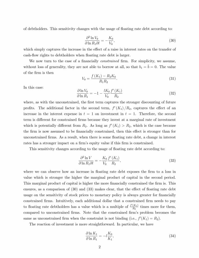
of debtholders. This sensitivity changes with the usage of floating rate debt according to:

∂2 lnV0∂ lnR1∂l

= −K0

V0, (30)

which simply captures the increase in the effect of a raise in interest rates on the transfer of

cash-flow rights to debtholders when floating rate debt is larger.

We now turn to the case of a financially constrained firm. For simplicity, we assume,

without loss of generality, they are not able to borrow at all, so that b1 = b = 0. The value

of the firm is then

V0 =f (K1)−R2K0

R1R2. (31)

In this case:∂ lnV0∂ lnR1

= −1− lK0

V0

f ′ (K1)

R2(32)

where, as with the unconstrained, the first term captures the stronger discounting of future

profits. The additional factor in the second term, f ′ (K1) /R2, captures the effect of an

increase in the interest expense in t = 1 on investment in t = 1. Therefore, the second

term is different for constrained firms because they invest at a marginal rate of investment

which is potentially different from R2. As long as f ′ (K1) > R2, which is the case because

the firm is now assumed to be financially constrained, then this effect is stronger than for

unconstrained firms. As a result, when there is some floating rate debt, a change in interest

rates has a stronger impact on a firm’s equity value if this firm is constrained.

This sensitivity changes according to the usage of floating rate debt according to:

∂2 lnV

∂ lnR1∂l= −K0

V0

f ′ (K1)

R2, (33)

where we can observe how an increase in floating rate debt exposes the firm to a loss in

value which is stronger the higher the marginal product of capital in the second period.

This marginal product of capital is higher the more financially constrained the firm is. This

ensures, as a comparison of (30) and (33) makes clear, that the effect of floating rate debt

usage on the sensitivity of stock prices to monetary policy is always greater for financially

constrained firms. Intuitively, each additional dollar that a constrained firm needs to pay

to floating rate debtholders has a value which is a multiple of f ′(K1)R2

times more for them,

compared to unconstrained firms. Note that the constrained firm’s problem becomes the

same as unconstrained firm when the constraint is not binding (i.e., f ′(K1) = R2).

The reaction of investment is more straightforward. In particular, we have

∂ lnK1

∂ lnR1= −lK0

K1

, (34)

2

if the firm is financially constrained, and

∂ lnK1

∂ lnR1= 0, (35)

if the firm is financially unconstrained. Equation (34) follows immediately from the fact that

for the constrained firm

K1 = N1 + b = f (K0)− rc (1− l)K0 − r1lK0 + b, (36)

and equation (35) follows from the fact that the investment of the unconstrained firm is

determined by the neoclassical investment rule f ′ (K2) = R2.

For r2 = rc = r1, we have that for a financially constrained firm

∂ lnK1

∂ lnR1∂l= −K0

K1

, (37)

while for an unconstrained firm this derivative is 0. Therefore, the effect of monetary policy

on investment is stronger for firms with high floating rate debt, l , especially if they are

financially constrained, i.e. have low K1.

B - Simulated Regressions of the Dynamic Model

B.1. Definition of VariablesThe definitions of the variables used in the dynamic model of Section 2.2 are standard

in the investment and capital structure literatures, and are given in Table A14.

[TABLE A14 ABOUT HERE]

B.2. Robustness of ResultsTable A15 displays regression results using simulated data from our dynamic model in

Section 2.2 in which we use floating rate debt over total assets as our proxy for exposure to

floating rate debt, as opposed to floating rate debt over total debt as in our main analysis.

All our results go through, although statistical and economic significance is slightly weaker.

[TABLE A15 ABOUT HERE]

C - Subsample Robustness of the Effect of Monetary Policy on Stock Prices

We start with the reaction of the aggregate CRSP value-weighted index between February

3

1994 and June 2008. Following Rigobon and Sack (2005), we focus on this period for two

reasons. First, starting in February 1994, the FOMC’s policy of announcing target rate

changes at pre-scheduled dates virtually eliminated the timing ambiguity associated with

rate changes prior to this date. Second, after June 2008, the Federal Reserve switched

from announcing a specific target rate to announcing a range for the target rate. Table A3

offers a comparison between the responses of equity prices to federal funds rate changes in

different samples, after discarding outliers as in Bernanke and Kuttner (2005). Columns 1

and 2 show that on the day of an FOMC announcement, a 100bp surprise increase in the

federal funds rate decreases stock prices by around 300bp when we look either at the value-

weighted returns or the individual returns of the entire CRSP universe between 1994 and

2008. This result is comparable to the numbers reported in Bernanke and Kuttner (2005).

Columns 3 and 4 show that the reaction of equity prices to surprise changes in monetary

policy is stronger in the sample of 2003—2008 than in previous years. However, the sign

and significance of the coeffi cient of surprise is the same for both samples. A comparison of

columns 4 and 5 reveals that firms in the sample for which we have bank debt usage data

have a reaction to monetary policy shocks very similar to that of the overall CRSP universe

during the 2003—2008 period.

[TABLE A3 ABOUT HERE]

D- Examples from 10-K files on hedging activities

The following two paragraphs are examples of the type of discussion on hedging activities

that we find in the 10-K files. In fiscal year 2008, BioFuel Energy Corp reports as follows:

We are subject to interest rate risk in connection with our bank facility.

Under the facility, our bank borrowings bear interest at a floating rate based,

at our option, on LIBOR or an alternate base rate. (...). In September 2007,

the Operating Company, through its subsidiaries, entered into an interest rate

swap for a two-year period. The contract is for $60.0 million principal with a

fixed interest rate of 4.65%, payable by the Operating Company and the variable

interest rate, the one-month LIBOR, payable by the third party.

Similarly, in fiscal year 2006 Netsmart Technologies reports:

In October 2005, we entered into a revolving credit and term loan agreement

with the Bank of America (...). This financing provides us with a five-year term

loan of $2.5 million. The term loan bears interest at LIBOR plus 2.25%. We

4

have entered into an interest rate swap agreement with the Bank for the amount

outstanding under the term loan whereby we converted our variable rate on the

term loan to a fixed rate of 7.1% in order to reduce the interest rate risk associated

with these borrowings.

E- Monetary Policy Surprise Calculation Procedure

Following Bernanke and Kuttner’s analysis, we define an event as either an FOMC meet-

ing or an announced change in the funds target rate. Kuttner (2001) and Bernanke and

Kuttner (2005) obtain the corresponding surprise change in the target rate by first calcu-

lating the change in the rate implied by the corresponding futures contract, given by 100

minus the futures contract price, and then scaling this result by a factor associated with

the number of days of the month in which the event occurred because the payoff of the

contract is determined by the average realized federal funds effective rate during the month.

Accordingly, the unexpected target rate change, for an event taking place on day d of month

m, is given by

∆iu =D

D − d(f 0m,d − f 0m,d−1),

where f 0m,d − f 0m,d−1 is the change in the current-month implied futures rate, and D is the

number of days in the month. To suppress the end-of-month noise in the federal funds rate,

the unscaled change in the implied futures rate is used as the measure of target rate surprise

when the event occurs on the last three days of a month. If the event happens on the first

day of a month, f 1m−1,D is used instead of f0m,d−1. The expected federal funds rate change is

defined as the difference between the actual change minus the surprise:

∆ie = ∆i−∆iu,

where ∆i is the actual federal funds rate change. The data for the decomposition of the

federal funds target rate changes can be obtained from Kenneth Kuttner’s webpage.66

F - The Effect of Bank Debt Usage on Monetary Policy Sensitivity of StockPrices

Table A4 presents the results of regression (22) using alternative specifications that be-

come more restrictive across columns. The first column of Table A4 contains the result from

a basic random-effects panel regression with no controls and suggests that a one standard

deviation (0.114) increase in our bank debt usage measure causes the stock price to increase

66http://econ.williams.edu/people/knk1/research

5

1.6 (= −14 ∗ 0.114) percentage points more in response to a 1 percentage point surprise de-

crease in the federal funds rate. To put this effect in perspective, the same surprise decrease

in the federal funds rate causes the stock price of the firm with the average amount of bank

debt over assets (7.22%) to increase about 4.97 percent on average.

[TABLE A4 ABOUT HERE]

Columns 2a-2c provide the same regression with different adjustments for well-known

risk factors in asset pricing. Column 2a repeats the same regression as column 1 with

the excess market return as an additional control variable and shows that the coeffi cient

of Surprise ∗ (BankDebt/At) remains very similar. Column 2b repeats the regression in

column 1 after replacing the dependent variable with the stock return in excess of that

predicted by the Capital Asset Pricing Model (CAPM), which corrects for the correlation

of individual stock returns with the aggregate market return. The coeffi cient of interest

(−10.5) is within one standard deviation of the coeffi cient in column 1 (−14.1). However,

the coeffi cient of Surprise changes significantly and actually turns positive. This does not

mean that a positive (contractionary) rate surprise causes an increase in the stock price of

the average firm. We observe this pattern because part of the market return on the FOMC

date can be attributed to monetary policy so the CAPM correction of returns prevents us

from measuring the full effect of monetary policy. The same pattern can also be observed

when we do the risk adjustment with the Fama-French three-factor model instead of CAPM,

as shown in column 2c. To circumvent this problem, we continue with the unadjusted returns

as in column 1 and use the CAPM beta as a control variable for the correlation of individual

returns with the market return in other regressions of Table A4. For the same reason, instead

of correcting returns using the Fama-French 3-factor model we use the firm characteristics

underlying the 3-factor model (size, market-to-book, CAPM beta) as control variables.67

Another advantage of this approach stems from the observation that firm characteristics

subsume the effect of the Fama-French risk factors in explaining stock returns, as discussed

in Daniel and Titman (1997) and Ferson and Harvey (1999).

In order to address potential identification issues, such as non-spherical disturbances

and omitted variables, we progressively add controls, industry fixed effects, both interacted

and uninteracted, standard errors clustered at the event-industry level, and firm fixed effects.

Non-sphericality would primarily affect the standard errors of our estimates rather than their

67For size, we use book value of assets, rather than market value of equity for two reasons. First, themarket equity size premium has declined significantly in the last three decades. Second, since Gertler andGilchrist (1994), balance sheet (rather than market) size has been widely used as a proxy of firms’financialconstraints, which is considered an important factor behind the transmission of monetary policy and thereforemore suitable for our purpose.

6

consistency, which is the main reason why we use clustered errors. However, omitted variables

can influence our inference by affecting both the standard errors and the consistency of our

estimates. Therefore, controls and firm-level fixed effects specifications aim at distinguishing

between bank debt being special, or bank debt users being special, for reasons that are not

captured in our basic regression in column 1 of Table A4. We also include an instrumental

variable analysis.

More specifically, column 3 introduces firm controls and year fixed effects and shows that

the coeffi cient in column 1 remains effectively unchanged. This is also robust to alternative

specifications, as shown in columns 4 to 8. In column 4, industry fixed-effects enter the

regression both interacted with surprise and uninteracted, with industries classified according

to Fama-French 48 sectors available from Kenneth French’s website, and errors are clustered

at the event-industry level to address possible time-and-cross-section heteroskedasticity in

the errors. Column 5 extends the definition of bank debt to include undrawn credit lines.

Another concern stems from the possibility that bank debt usage is caused by cash flow

risk, financial constraints or the interest rate sensitivity of firms’demand and our results

reflect the importance of these factors rather than bank debt usage, so in column 6 we

introduce measures that control for these factors. We follow Faulkender (2005) and measure

the interest rate sensitivity of firms’operating profits as the correlation between quarterly

firm earnings before interest, tax, depreciation and amortization (EBITDA) and three-month

average LIBOR rates. We introduce cash flow volatility and CAPM beta as controls for

firm risk, and cash holdings as a measure of the ability of the firm to withstand liquidity

shocks associated with monetary policy. Finally, to capture financing constraints, we follow

Hadlock and Pierce (2010), who show that firm size and age are very useful predictors of

the severity of financial constraints, and introduce a measure based solely on these two firm

characteristics.68 We call this measure of financial constraints the HP index. To further deal

with this concern, Column 7 replaces industry fixed effects with firm fixed effects to capture

unobserved time invariant omitted firm characteristics. Overall the coeffi cient of bank debt

usage barely changes, which adds robustness to the evidence that bank debt usage makes

firms more responsive to monetary policy shocks.

Column 8 includes an instrumental variable regression with fixed effects to deal further

with the potential endogeneity problem of bank debt usage. Following Faulkender and

68We use Hadlock and Pierce’s estimates for 2000-2004 from Table 6 in their paper because this periodis closer to our sample. The HP index is calculated as (-0.548*Size) + (0.025*Size^2) —(0.031*Age), wheresize is the log of inflation adjusted (to 2004) book assets, and age is the number of years for which thefirm has stock returns in CRSP to ensure that we have few missing observations. An alternative measurecan be derived using the IPO date, but this leads to multiple missing observations, though the results arequalitatively similar. In calculating this index, size is replaced with log($4.5 billion) and age with thirty-sevenyears if the actual values exceed these thresholds.

7

Petersen (2006) and Santos and Winton (2008) we instrument for bank debt usage using

proxies for firm visibility and firm uniqueness. These authors use these proxies to instrument

for firm access to corporate bond markets and argue that firms that are highly visible and less

unique are more likely to be rated. As proxies for visibility, they introduce firms’membership

of the S&P 500 index or of the New York Stock Exchange (NYSE). As a proxy for uniqueness,

they use a measure of the number of firms in their same industry other than itself that

have credit ratings. We instead use them as instruments for bank debt usage following

the argument that firms that do not have access to bond markets are likely to be stronger

users of bank debt. Our last instrument relies on the observation that banking regulation

limits the amount of unsecured loans a bank can issue (Ivashina (2009)). Consistent with

this observation, Altman, Gande, and Saunders (2010) find that about 70 percent of the

bank loans to corporations are secured, in contrast to 3 percent of bonds. Therefore, we

would expect that the collateral of a firm is an important determinant of how much the

firm can borrow from a bank, and hence use tangibility as an additional instrument.69 We

find that while we lose statistical significance, the coeffi cients of the regression are effectively

unchanged and the Hausman test cannot reject the hypothesis that they are the same,

suggesting that endogeneity is not a big concern.

Finally, column 9 provides the same specification as in column 7 but replaces bank

debt with floating rate debt. While the statistical significance of floating rate debt drops

somewhat, as expected due to the points mentioned in the data section, it is similar in size

to the coeffi cient of bank debt in column 7 and still statistically significant.

A possible concern in Table A4 is that bank debt may be proxying for the use of short-

term debt. This concern finds support in the descriptive statistics reported in Table IV which

shows that bank debt users have a higher percentage of short-term debt than nonbank-debt

users (3.71 percent versus 1.09 percent, calculated as a share of total assets) and that the

Pearson pair-wise correlation between these two variables is 0.27. For example, to the extent

that changes in monetary policy affect primarily the short end of the yield curve, one can

expect firms with a shorter average maturity of debt to be more sensitive to increases in

interest rates.

To test this hypothesis, we rewrite the specification provided in equation (22) in terms

of short-term debt divided by the book value of assets, STDebt/At. Formally, the complete

69Because we are interested in how bank debt usage affects firms’sensitivity to monetary policy shocksand because this term in our regression is non-linear, given by Surpriset ∗ (BankDebt/At)i,t−1, we cannotuse the traditional instrumental variable approach where the first stage estimates of (BankDebt/At)i,t−1 areused to replace our endogenous variable in the second stage, which is dubbed "the forbidden regression" inthe literature. Therefore, we use an alternative approach suggested in Angrist and Pischke (2009, Ch. 4)where we use Surpriset ∗ (Instrument)i,t−1 as an instrument for Surpriset ∗ (BankDebt/At)i,t−1 .

8

regression specification is:

Rett = β0 + β1Surpriset + β2 (BankDebt/At)t−1 + β3 (STDebt/At)t−1

+β4Surpriset ∗ (BankDebt/At)t−1 + β5Surpriset ∗ (STDebt/At)t−1

+γControlst−1 + λSurpriset ∗ Controlst−1 + εt. (38)

Table A11 provides the empirical results of this test. Columns 1 and 2 show the results

of a version of regression (38) in which the terms containing (BankDebt/At)t−1 are removed.

We observe that the amount of short-term debt in a firm’s balance sheet is not significantly

associated with the strength of the sensitivity to surprises in the federal funds rate. The

coeffi cient in column 1 (−10.30) is not only statistically insignificant but also economically

very small: one standard deviation in short-term debt usage leads to only a (10.30 ∗ 0.05 =)

0.5 percentage point increase in the sensitivity to monetary policy of stock prices, a far lower

figure than the 1.6 percentage points for bank debt usage. Introducing additional controls in

column 2 makes this effect even smaller. Columns 3 and 4 provide a complete specification of

(38), including bank debt, both interacted and not interacted with Surprise. The coeffi cient

β5 remains insignificant, while the coeffi cient β4 retains the sign, size, and significance of the

specifications reported in Table A4. We conclude that the higher sensitivity of bank debt

users to federal funds rate surprises is not due to their higher exposure to short-term debt.

Finally, one potential concern is that our bank debt usage variable, BankDebt/At, might

be correlated with other leverage variables and our results reflect the importance of debt

in general rather than bank debt in particular. One way we address this concern is by

adding book leverage directly in Table A4. As another way to address the same issue, we

normalize total bank debt with total debt to create an alternative measure of bank debt

usage, BankDebt/Debt. We use this new measure to replace our original measure and

repeat the regressions in Table A4. The new results, presented in Table A12 in the appendix

confirm our results from Table A4. In particular, we find that a one standard deviation in

BankDebt/Debt (0.40) leads to approximately a (0.40 ∗ 3 =) 1.2 percentage point increase

in the responsiveness of stock prices to monetary policy surprises, which is in the ballpark

of our previous result (1.6 percentage points) using BankDebt/At.70 Hence, we continue to

use BankDebt/At in the following analysis.

G - Effect of Hedging: Controlling for Financial Frictions

70As before, the floating rate debt coeffi cient is somewhat smaller due to mismeasurement. A similar issuealso appears when we include undrawn credit lines in column 4 because there are some firms in our samplethat have very little debt but very large undrawn credit lines.

9

One concern in our previous regressions is that the estimates might be biased due to

an omitted variable bias associated with the relationship between financial constraints and

firms’hedging behavior. Some theories predict that hedging activities are positively related

to the severity of financing constraints. If external finance is costly, firms may find it optimal

to hedge against low cash flow realizations to avoid having to forgo positive net-present-value

(NPV) projects (Froot, Scharfstein, and Stein (1993)) or to avoid nonlinear costs of financial

distress (Stulz (1984)).71 The empirical evidence, however, does not provide support for this

prediction, and has documented that firms that are more likely to face financial constraints,

such as small firms, are less likely to manage risk (Stulz (1996)).72 Motivated by these

findings, Rampini, Sufi, and Viswanathan (2014) introduce and test a theory that suggests

there is a trade-off between hedging and financing, because both activities compete for the

same collateral. In equilibrium, firms that are more financially constrained hedge less. The

important role of financing constraints in firms’willingness and ability to hedge suggests that

one should control for financial constraints and how these constraints interact with both the

ability to raise debt and to hedge.73

To deal with this concern, we study how much of the effect of hedging survives after

controlling for financial frictions, which we measure using firm age and the HP index. In

particular, we estimate an expanded version of regression (23)

71Other motivations for the use of hedging have to do with corporate governance and managerial incentives(Chava and Purnanandam (2007)), and with market timing (Faulkender (2005)). More generally, the valuecreation of hedging has been examined by Nance, Smith, and Smithson (1993), Mian (1996) and Grahamand Rogers (2002).72Columns 5 and 6 of Table A2 show that this is the case also in our sample. Larger, rated, more profitable

and less financially constrained (low HP index) firms are more likely to hedge than their smaller, unrated,less profitable or more financially constrained counterparts.73One important question is why most bank lending arrangements involve a floating rate instead of a fixed

rate despite the fact that many firms hedge the interest rate risk associated with these loans. One answercould arise from the trade-off between firms’needs and banks’cost of capital. A firm that wants to borrowat a fixed rate may have limited access to other fixed-rate sources of financing, such as bonds, whereas thebank might prefer to lend at floating rates, in which case hedging bridges the gap between the desire of thebank and the firm. As discussed by Vickery (2008), there are at least two reasons why banks might preferto lend at floating rates. First, rising interest rates can cause deposit outflows from the banks and it iscostly for banks to replace these outflows with other sources of financing. Lending at a floating rate wouldprovide a partial hedge against these outflows. Second, floating rate business loans can be used to hedge thematurity mismatch between deposits and long-term mortgage loans.

10

Rett = β0 + β1Surpriset + β2Surpriset ∗ (BankDebt/Att−1)

+ β3Surpriset ∗ (BankDebt/At)t−1 ∗Hedget+ β4Surpriset ∗ (BankDebt/At)t−1 ∗ FinFrictionst−1+ λ1Surpriset ∗ Controlst−1 ∗Hedget+ λ2Surpriset ∗ Controlst−1 ∗ FinFrictionst−1+Uninteracted terms and Second Order Interactions+ εt (39)

and check if β3, the coeffi cient of Surpriset ∗ (BankDebt/At)t−1 ∗Hedget, remains similar towhat we have calculated before in Table V and whether it still eliminates the full effect of the

Surpriset ∗ (BankDebt/At)t−1, i.e., β3 + β2 = 0. Columns 1 and 2 of Table A13 show that

the estimates of β3 have a magnitude very similar to the one we have calculated in Table V

for the coeffi cient on the triple interaction term Surpriset ∗ (BankDebt/At)t−1 ∗Hedget andthat it nullifies the effect of Surpriset ∗ (BankDebt/Att−1) . Similar evidence is obtained in

columns 3 and 4 when we use floating rate debt instead of bank debt. These results suggest

that the floating rate channel is a unique and distinct channel that works separately from

possible effects of financial frictions.

H - Description of Tests based on Balance Sheet Variables

In this Appendix, we describe in detail the empirical tests discussed in Section 5.

Interest Coverage Ratio TestsWe compute the interest coverage ratio at the quarterly level as the sum of interest

expenses (Compustat item, XINTQ) and cash flow divided by interest expenses, where cash

flow is equal to earnings before extraordinary items (IBQ) plus depreciation (DPQ). We test

whether a higher bank debt usage as a share of total assets increases the responsiveness

of firms’interest rate coverage ratios following monetary policy actions, due to the higher

likelihood of this debt being floating rate. We use the following empirical specification:

∆CoverageRatiot−1,t+x = β0 + β1Changet

+β2 (BankDebt/At)t−1 + β3Changet (BankDebt/At)t−1

+γControlst−1 + λChanget (Controlst−1) + εt, (40)

where Changet is the cumulative quarterly change in the interest rate, as in Ashcraft and

Campello (2007) and Jiménez, Ongena, Peydró, and Saurina (2012, 2014), instead of the

11

cumulative surprise component because cash flow and the interest rate expense on existing

debt is not forward-looking the way stock prices are.74 Our firm-level controls include book

leverage, firm size, market-to-book ratio, profitability, interest rate sensitivity, and short-

term debt. We include firm and year-quarter fixed effects, and we cluster errors at the

industry-quarter level.75

The dependent variable (∆CoverageRatiot−1,t+x) is calculated as the change between

the coverage ratio in the quarter before the monetary policy shock and x ∈ {1, 2, 3, 4, 5, 6}quarters ahead. The timing of effects of the floating rate channel is influenced by the fre-

quency with which interest rates of floating rate bank loans are reset to adjust to movements

in the reference rate. Because this frequency can range from 1 day to 1 year (Inklaar and

Wang (2013)), the effects might occur with a lag of several quarters, although a majority

of commercial and industrial (C&I) loans have a resetting frequency of one month or less,

according to the Federal Reserve’s Survey of Terms of Business Lending.

As in Sections 4.2 and 4.4, we restrict our sample to include firms that have outstanding

variable rate debt equivalent to at least 1% of total assets to eliminate firms that may be using

interest-rate derivatives for speculative purposes, and we run specification (40) separately

for subsamples of hedgers and non-hedgers.

Cash Holdings TestsWe compute the change in cash holdings as the difference between total cash and short-

term investments at the end of quarter t + x (where x ∈ {1, 2, 3, 4, 5, 6}) and at the end ofquarter t−1, scaled by total assets at the end of the quarter t−1. Changes in cash holdings are

expressed in basis points, and we use the same regression specification as (40). Firm controls

are taken from the empirical literature that focuses on corporate cash accumulation (Bates,

Kahle and Stulz (2009)), and include firm size, leverage, market-to-book ratio, and cash flow

risk. We test whether the impact of bank debt usage on the sensitivity of cash holdings

to monetary policy (coeffi cient β3) is significantly stronger for financially constrained firms

than for unconstrained firms in the sample of unhedged firms, and whether this difference

is absent or is at least significantly smaller in the sample of hedged firms. We classify firms

as financially constrained (unconstrained) if their value of the Hadlock and Pierce (2010)

(HP) index is above (below) the median, and report the difference between the estimates

of β3 across constrained and unconstrained firms, within each of the subsamples of hedgers

74This argument also holds for other balance sheet variables in this section, as they are more likely torespond to the anticipated component of monetary policy changes as well because adjustment costs preventthem from reacting rapidly to changes in expectations about future policy rates, particularly when the changein the expectation happens shortly before the FOMC announcement. Still, our results in this section remainqualitatively similar when we use the sum of the monetary policy surprises on the FOMC announcementsdates in a given year, as in Gorodnichenko and Weber (2014).75Year-quarter fixed effects also control for possible seasonality occurring at the quarterly frequency.

12

and non-hedgers, and also report the statistical significance of the difference.76 Results are

analyzed for horizons of four and six quarters.

Inventory Investment TestsWe follow Kashyap, Lamont and Stein (1994) and adopt their empirical specification

for our inventory investment regressions, which we augment to introduce monetary policy

changes, bank debt usage, and our firm level controls:

ln

(Inventoriest+xInventoriest−1

)= β0 + β1Changet

+β2 (BankDebt/At)t−1 + β3Changet (BankDebt/At)t−1

+γControlst−1 + λChangetControlst−1

+ ln

(Salest,t+x

Salest−x−1,t−1

)+ ln(

Inventoriest−1Salest−1

) + εt. (41)

Our firm-level controls include, as before, book leverage, firm size, market-to-book ratio,

profitability, interest rate sensitivity, and short-term debt. We add, following Kashyap,

Lamont and Stein (1994), the cash to total assets ratio at the end of quarter t−1, separately

and interacted with change, and also the difference between the log of total sales during

quarters t to t+ x and the log of total sales during quarters t− x− 1 to t− 1, and the log of

the inventory to sales ratio at the end of quarter t − 1. We express our dependent variable

in basis points. We include firm and year-quarter fixed effects, and we cluster errors at the

industry-quarter level. Results are analyzed for horizons of four and six quarters.

Sales TestsWe interpret sales, in line with existing literature, as a proxy for firm-level output (Gertler

and Gilchrist (1994), Bond, Elston, Mairesse, and Mulkay (2003)). We employ empirical

specification (40) and use the difference between the log of total sales during quarters t to

t+ x and the log of total sales during quarters t− x− 1 to t− 1 as our dependent variable.

As before, we introduce year-quarter fixed effects, which also control for possible seasonality

occurring at the quarterly frequency.

Fixed Investment TestsTo test our prediction on fixed investment, we expand our baseline empirical specification

(40) to include the main factors that have been identified in the empirical literature to matter

for firm investment (Eberly, Rebelo and Vincent (2012)). These are Tobin’s Q, proxied by

76As explained in Section 4.4, we choose the HP measure because Hadlock and Pierce (2010) show thatother indices have very little power to predict financial constraints, and any power they have comes fromfirm size and age, the two variables they use to create their composite HP index.

13

the market-to-book ratio, cash flow, and lagged investment. We run the following regression:

ln

(Kt+x

Kt−1

)= α0 + α1Changet + α2 (BankDebt/At)t−1 + α3Changet (BankDebt/At)t−1

+λ (FirmControls)t−1 + γChanget (FirmControls)t−1

+α4Qt + α5

(CFtKt

)+ α6

(It−1Kt−1

)+ εt, (42)

where our dependent variable is computed as the difference between the log of total fixed

capital (measured as property, plant and equipment) x quarters ahead, and the log of capital

one quarter before the monetary policy event. We express our dependent variable in basis

points. Our firm-level controls also include book leverage, firm size, profitability, interest rate

sensitivity, and short-term debt, all interacted with Changet and also introduced separately.

We include firm and year-quarter fixed effects, and we cluster errors at the industry-quarter

level.

I - Bank Lending Channel vs Floating Rate Channel

According to the estimations in Holod and Peek (2007), a one percentage point permanent

rate hike would be associated with a 0.01 (for publicly-held banks) to 0.1 percentage point

(for privately-held banks) decrease in C&I loans as a fraction of total bank assets over a four

quarter period. Moreover, C&I loans are about 10 percent of total assets for both public

and private banks, and public banks hold about 80 percent of total assets (Nichols, Wahlen,

and Wieland (2009)). Therefore, the weighted average effect is a 0.3 percent decrease in

C&I loans over a four quarter period ((0.01/0.1)*0.8+(0.1/0.1)*0.2=0.3). This result is

also in line with Oliner and Rudebusch (1996): over eight quarters they find a 0.6 percent

decrease in C&I loans to small firms who hold half the bank loans whereas no loan decline

is observed for large firms, implying a 0.3 percent decrease for total loans. Moreover, since

this effect is the same as the effect from Holod and Peek (2007) over the first year, we can

conclude that this is the long-run effect of a permanent increase in the federal funds rate.

Overall, this suggests that a firm that usually borrows $100 from the bank will experience

a cumulative $0.3 shortfall if the federal funds rate increases by one percentage point. This

effect includes any amplification mechanism that works through bank balance sheets. Of

course, this effect might be an upper bound for the true supply effect because part of the

effect can be attributed to the potential decline in loan demand due to reduced demand

for goods and services associated with the tightening of monetary policy. Moreover, Oliner

and Rudebusch (1996) find that loans to large firms actually increase after a tightening,

suggesting a reallocation of credit from small firms to large firms that further alleviates the

14

effects of the bank lending channel.

How does this compare to the floating rate channel? A one percentage point rate hike

would increase the interest expense by $1 on a $100 loan. However, some loans are fixed rate

and some floating rate loans are hedged, which we will take into account. Since the papers

about the bank lending channel in the previous paragraph focus on C&I loans, we will do

the same here. As shown in Vickery (2008), about 70 percent of total bank loans in the

Federal Reserve’s survey of business lending is made at a floating rate which is close to what

Figure 2 suggests (about 75 percent) in our sample. If we continue with the same assumption

that half of C&I loans are made to small businesses this would imply that about 65 percent

of C&I loans to small businesses are at a floating rate (0.65*0.5+0.75*0.5=0.7). Moreover,

we find that firms that do not use hedging derivatives hold about 30 percent of the loans

in our sample, where almost all firms are large according to the definition of the Quarterly

Financial Report for Manufacturing, Mining, and Trade Corporations (QFR) used by Oliner

and Rudebusch (1996), which has a cutoffof $25 million in total assets to qualify firms as large

in 2014. Small and medium sized firms usually make little use of hedging derivatives (Vickery

(2008)). Therefore, as an initial approximation, we assume that no small firm hedges. As

a second approximation, we will assume that small firms have the same hedging behavior

as the firms with less than 25 million dollars in assets in our sample (37 percent in terms

of total loan size) which is an upper bound for hedging derivative usage because these firms

are on the upper tail of the size distribution. Using these numbers, we calculate the total

percentage of C&I loans that are floating rate and unhedged as a number between 0.32 and

0.44 (0.65*(1-0.37)*0.5+0.75*0.3*0.5=0.32 and 0.65*1*0.5+0.75*0.3*0.5=0.44). Therefore,

the average cash shortfall after the one percentage point rate hike would be between $0.32

and $0.44 on a $100 loan over four quarters, or $0.64 to 0.88 over two years, assuming the

effect on the interest expense persists over this time horizon, which seems to be the case

according to unreported regressions in which we study the effect of bank debt usage and

hedging on the response of the interest expense of firms to monetary policy.77

77One implicit assumption is that the rate on the C&I loans is reset frequently. According to the Surveyof Terms of Business Lending of November 2006, 27 percent of the C&I loans are subject to repricing at anytime, 28 percent of the loans have daily repricing, and 23 percent of the loans have a repricing period of 2-30days.

15

 

TABLES AND FIGURES

 

Figure 1

The relation between the Federal Funds Target Rate and Floating-Rate Debt Reference Rates This figure displays the relation between two of the most common reference rates used in floating rate loans, the 3-Month London Interbank Offered Rate (LIBOR) and the Bank Prime Loan Rate, and the Federal Funds Target Rate, from January 1986 until January 2015. The data is from the Federal Reserve Bank of St. Louis FRED Economic Data.

Figure 2 The relation between bank debt and floating-rate debt

This figure displays the relation between bank debt and floating-rate debt as a percentage of a firm’s total debt. Firms are grouped in the horizontal axis according to bank debt as a percentage of total debt. The vertical axis shows the corresponding percentages of floating-rate debt as a percentage of total debt.

 

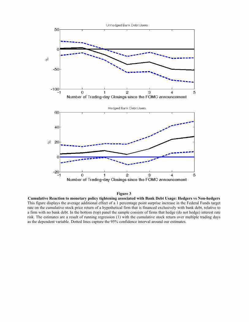
Figure 3

Cumulative Reaction to monetary policy tightening associated with Bank Debt Usage: Hedgers vs Non-hedgers This figure displays the average additional effect of a 1 percentage point surprise increase in the Federal Funds target rate on the cumulative stock price return of a hypothetical firm that is financed exclusively with bank debt, relative to a firm with no bank debt. In the bottom (top) panel the sample consists of firms that hedge (do not hedge) interest rate risk. The estimates are a result of running regression (1) with the cumulative stock return over multiple trading days as the dependent variable. Dotted lines capture the 95% confidence interval around our estimates.

 

 

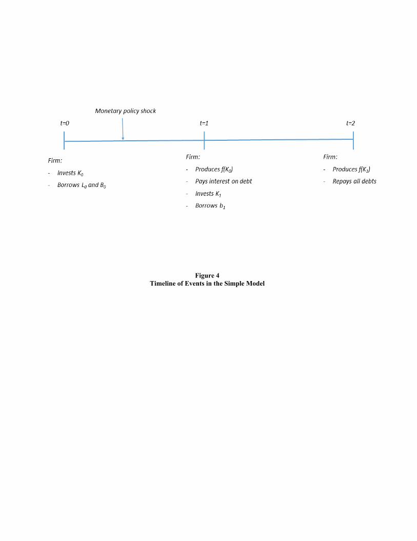
Figure 4

Timeline of Events in the Simple Model

 

 

Table I Dynamic Model Calibration – Parameter Value Choices

 

 

Table II The Effect of Monetary Policy – Simulated Data

Panel A of this table examines how monetary policy affects firms’ stock returns and how this effect varies with floating rate debt usage and financing constraints. Not displayed in this table are some of the lower order combinations of the triple interaction variable (Constrained*Surprise *Floating Rate/ Total Debt), the constant term, and controls. Column 3 displays a regression in which the costs of distress are 33% lower than in the benchmark calibration. Panel B of this table examines how monetary policy affects firms’ investment and how this effect varies with floating rate debt usage and financing constraints. Not displayed in this table are some of the lower order combinations of the triple interaction variable (Constrained*Change *Floating Rate/ Total Debt), the constant term, and Tobin’s Q. Surprise, Change, Stock Return and Net Investment/K are expressed in basis points. The definitions of all the variables used are described in detail in Appendix B. Parentheses contain t-statistics. The asterisks denote *** for p<0.01, ** for p<0.05, * for p<0.1.

Panel A. Effect on Stock Returns Dep variable: Stock Returnt (1) (2) (3) Surprise -19.55*** -15.08*** -15.04*** (-54.41) (-46.17) (-76.62) Surprise *Floating Rate/ Total Debt -21.58*** -23.12*** -15.99*** (-37.14) (-44.21) (-43.17) Constrained*Surprise *Floating Rate/ Total Debt -7.25*** -4.23*** -3.54***

(-6.83) (-4.43) (-5.22) Controls NO YES NO Distress Costs Benchmark Benchmark Low R-squared 0.19 0.24 0.24 Observations 38,000 38,000 38,000

Panel B. Effect on Investment Dep variable: Net Investmentt, t+x/Kt-1 4 Quarters Ahead 6 Quarters Ahead (1) (2) (3) (4) Change -0.19*** -0.47*** -0.46*** -0.64***

(-6.30) (-14.72) (-15.02) (-20.07) Change *Floating Rate/ Total Debt 0.02 -0.24*** 0.19*** 0.02

(0.47) (-4.71) (3.87) (0.34) Constrained*Change *Floating Rate/ Total Debt

-0.12 -0.22** -0.42*** -0.49***

(-1.40) (-2.46) (-4.71) (-5.42) Controls NO YES NO YES R-squared 0.01 0.04 0.01 0.03 Observations 38,000 38,000 38,000 38,000

 

 

Table III The Effect of Monetary Policy on Financial Distress – Simulated Data

This table examines how monetary policy affects firms’ financial distress likelihood (column (1)), costs of financial distress (column (2)), and the interest rate coverage ratio (column (3)), and how these effects vary with floating rate debt usage and financing constraints. Not displayed in this table are some of the lower order combinations of the triple interaction variable (Constrained*Surprise *Floating Rate/ Total Debt), the constant term, and controls. All dependent variables and Change are expressed in basis points. The definitions of all the variables used are described in detail in Appendix B. Parentheses contain t-statistics. The asterisks denote *** for p<0.01, ** for p<0.05, * for p<0.1.

Dep variable: Covenant Violation

Likelihood

Costs of Financial Distress

Interest Rate Coverage Ratio

(1) (2) (3) Change 1.48*** 0.08 0.18 (5.18) (1.55) (0.72) Change *Floating Rate/ Total Debt 0.21 0.64*** 13.36*** (0.674) (6.39) (29.79) Constrained*Change *Floating Rate/ Total Debt 2.38*** 1.56*** 2.62***

(2.58) (8.48) (3.19) R-squared 0.19 0.24 0.16 Observations 38,000 38,000 38,000

 

 

Table IV Descriptive Statistics

This table provides summary statistics for the entire sample and for different subsamples. The entire sample consists of U.S. firms covered by Capital IQ, CRSP, and Compustat from 2003 to 2008 with December fiscal year-end, excluding utilities (SIC codes 4900-4949) and financials (SIC codes 6000-6999). We remove firm-year observations with negative revenues, missing information on total assets, or a value of total assets under 10 million. We also discard penny stocks, defined as those with a price of less than $5. After the above filters, the sample contains 9,746 firm-year observations comprising 2,368 unique firms. Complete variable definitions are given in the appendix. All variables are winsorized at the 1% level in both tails of the distribution, and total assets are expressed in terms of year-2000 dollars. See Table A1 for variable definitions.

(1) (2) (3) (4)

Entire Sample

Leveraged Firms w/out Bank Debt

Leveraged Firms with Bank Debt Hedgers Nonhedgers

Mean SD Mean SD Mean SD Mean SD Term Loans/At 3.95% 9.02% 0.00% 0.00% 8.93% 12.70% 5.09% 8.88%

Drawn Credit Lines/At 3.09% 6.55% 0.00% 0.00% 6.12% 8.51% 5.06% 7.36% Bank Debt /At 7.22% 11.66% 0.00% 0.00% 15.52% 14.33% 10.33% 11.01% Bank Debt / Total Debt 37.51% 40.07% 0.00% 0.00% 50.35% 36.26% 58.89% 37.97% Floating-Rate Debt/At 9.77% 13.44% 1.59% 5.86% 15.37% 15.77% 10.04% 11.73%

Float-Rate Debt / Tot. Debt 38.31% 40.47% 8.95% 24.65% 47.04% 38.14% 50.62% 41.26% Undrawn Credit Line/At 9.85% 10.56% 8.19% 9.89% 12.99% 9.61% 11.11% 10.95% (Bank Debt + Und CL)/At 17.14% 16.64% 8.19% 9.89% 28.51% 16.89% 21.43% 15.36% Short-Term Debt /At 2.55% 5.15% 1.85% 4.25% 3.65% 6.13% 3.71% 5.76%

Profitability 4.94% 15.73% 4.35% 16.46% 8.91% 7.24% 4.31% 16.40% Size (Total Assets, Million $) 4,274.32 23990 5,404.67 20,292.93 5,071.905 23,784.68 4,677.73 32,800.7 Book Leverage 28.15% 29.58% 26.87% 29.38% 45.19% 27.21% 31.07% 27.71%

Earnings-Interest Rate Sensitivity -13.23% 35.46% -11.82% 36.96% -15.63% 33.43% -12.98% 34.44% Rated Dummy 32.98% 47.02% 36.23% 48.08% 57% 49.52% 28.76% 45.27% Market-to-Book Assets 1.98 1.57 2.13 1.61 1.42 0.92 1.79 1.38 Cash/At 22.35% 24.26% 27.19% 23.31% 7.44% 9.83% 17.44% 22.07%

CAPM Beta (Monthly) 1.32 1.20 1.37 1.23 1.11 0.93 1.35 1.24 Cash Flow Volatility 1.11% 0.49% 1.14% 0.44% 0.95% 0.42% 1.10% 0.48% Hadlock-Pierce Fin. Con. Measure -2.85 0.59 -2.89 0.61 -3.12 0.49 -2.82 0.57 Age 16.78 17.01 18.08 18.95 20.20 19.31 16.63 15.72

Hedging Dummy 34.80% 47.63% 26.46% 44.12% 100.00% 0.00% 0.00% 0.00% Hedging*(Bank Debt /At) 4.22% 10.18% 0.00% 0.00% 15.52% 14.33% 0.00% 0.00% Hedging*( Floating-Rate Debt/At) 5.75% 12.11% 0.71% 3.94% 15.37% 15.77% 0.00% 0.00%

Firm’s lenders’ characteristics: Bank Size (ln(assets)) 19.80 1.92 19.65 2.05 Tier 1 Capital Ratio 8.39% 0.65% 8.46% 0.82% Deposit Ratio 51.03% 7.84% 53.90% 9.55%

Liquidity Ratio 22.47% 4.17% 21.32% 5.50%

Observations (annual) 9,746 9,746 2,509 2,509 2,463 2,463 2,647 2.647

Quarterly data Interest Rate Coverage Ratio 0.14 0.19 0.12 0.18 0.22 0.20 0.14 0.18 Inventory (quarterly growth %) 2.02% 21.70% 2.37% 23.10% 1.71% 17.96% 1.73% 19.03% Sales (quarterly growth %) 2.16% 21.1% 2.40% 21.19% 1.51% 17.48% 2.04% 21.67% Prop. Pla. & Equip. (q. growth %) 2.13% 5.42% 2.15% 5.50% 1.80% 5.12% 2.05% 5.09%

Observations (quarterly) 45,694 45,694 11,932 11,932 10,117 10,117 11,645 11,645

 

 

Table V

The Role of Bank Debt Usage and Interest Rate Risk Exposure in the Transmission of Monetary Policy This table examines how firms’ bank and floating rate debt usage impacts the effect of monetary policy on stock prices, and how this impact varies with firms’ hedging activity. Hedgers are defined on a yearly basis as those firms that report having swapped their interest rate from floating to fixed in their 10-K annual reports. Only firms with floating rate debt constituting more than 1% of total assets are included. Bank Debt/At is defined as bank debt (term loans plus drawn revolving credit) over the book value of assets (At). FloatingRateDebt /At is defined as floating rate debt over the book value of assets (At). All regressions also include an unreported constant term, as well as ln(assets), book leverage, profitability, market-to-book, interest rate sensitivity, and their interaction with surprise. All firm characteristics are lagged by one year and winsorized at 1%. Parentheses contain t-statistics. The asterisks denote *** for p<0.01, ** for p<0.05, * for p<0.1. (1) (2) (3) (4) (5) (6) (7) (8)

Panel A - Main Variables ALL Non-

Hedgers Hedgers Non-

Hedgers Hedgers ALL Non-

Hedgers Hedgers Non-

Hedgers Hedgers

Surprise -6.04** -4.10*** -8.62*** -5.08* -6.83** -6.20*** -4.59*** -8.22*** -5.76** -6.34** (-2.54) (-4.07) (-9.05) (-1.91) (-2.35) (-2.63) (-4.76) (-8.96) (-2.20) (-2.16)

BankDebt/At 1.28** 0.35 0.26 0.13 1.94*** (2.38) (0.86) (1.14) (0.13) (3.12)

FloatingRateDebt /At 1.03** 0.25 0.21 0.77 1.19** (2.06) (0.65) (0.96) (0.84) (2.14)

Surprise *(BankDebt/At) -13.50* -25.18*** 1.41 -38.02*** 3.45 (-1.76) (-3.04) (0.26) (-3.09) (0.38)

Surprise *(FloatingRateDebt /At) -14.70* -20.81*** -2.72 -30.79** -3.71 (-1.92) (-2.60) (-0.53) (-2.36) (-0.40)

Surprise*(BankDebt/At)*Hedging 26.71*** 41.46*** (2.85)

(2.71)

Surprise*(FloatingRateDebt /At)*Hedging 17.78* 27.07* (1.90) (1.74)

(continues on the next page)

 

 

(ctd from previous page) (1) (2) (3) (4) (5) (6) (7) (8)

Panel B - Surprise*Other variables ALL Non-

Hedgers Hedgers Non-

Hedgers Hedgers ALL Non-

Hedgers Hedgers Non-

Hedgers Hedgers

Surprise *log(Assets) -1.32** -1.95*** -0.55 -1.30** -1.62** -0.77 (-2.34) (-2.69) (-0.77) (-2.35) (-2.21) (-1.11) Surprise *Book Leverage -0.32 5.85 -6.20 0.64 5.73 -4.14 (-0.09) (1.18) (-1.36) (0.18) (1.13) (-0.91) Surprise *Market-to-Book 0.81 -0.22 2.18 0.85 -0.12 2.19 (0.80) (-0.17) (1.60) (0.83) (-0.10) (1.61) Surprise *Profitability -18.28 -16.22 -22.98 -18.04 -16.65 -23.07 (-1.63) (-1.34) (-1.06) (-1.62) (-1.39) (-1.06) Surprise *Int. Rate Sensitivity -7.63 -9.21 -5.61 -7.76 -9.77* -5.84 (-1.50) (-1.58) (-0.89) (-1.54) (-1.69) (-0.92)

Test for the coefficients of

Surprise*(Other variables)*Hedging

are jointly zero (p-value) 0.19 0.39

Firm Controls YES NO NO YES YES YES NO NO YES YES

Firm FE YES NO NO YES YES YES NO NO YES YES

Surprise*Firm Controls YES NO NO YES YES YES NO NO YES YES

Cluster (Fed event*IndustryFF48) YES NO NO YES YES YES NO NO YES YES

Observations 24,123 11,796 12,335 11,788 12,335 24,123 11,796 12,335 11,788 12,335

 

 

Table VI The Role of Interest Rate Risk Exposure in the Transmission of Monetary Policy: Instrumental Variables Analysis

All variables are as defined in Table IV. Column (1) is the fixed effects regression for the sample of firms that have data on lagged hedging dummy and column (3) is the fixed effects regression for the sample of firms that have data on tax convexity, our instrument for hedging from Graham and Smith (1999) and Campello, Lin, Ma, Zou (2011). Column (2) uses lagged hedging dummy as instrument for hedging. Column (4) uses the variables underlying the convexity measure, excluding Vol, whereas column (5) uses all variables as instruments. Column (6) uses the tax convexity measure directly, as given in the text. Column (7) uses both the lagged hedging dummy and the tax convexity measure. Only firms with floating rate debt constituting more than 1% of total assets are included. A constant, non-interacted terms, and the policy surprise interacted with firm size, book leverage, profitability and the market-to-book ratio are included but not reported. All firm characteristics are lagged by one year and winsorized at 1%. Parentheses contain t-statistics. The asterisks denote *** for p<0.01, ** for p<0.05, * for p<0.1. The coefficient of Surprise in columns (4) to (6) are not negative because the linear first stage regression does not restrict hedging between zero and one.

Panel A: Bank Debt (1) (2) (3) (4) (5) (6) (7)

OLS IV OLS IV1 IV2 IV3 IV L.hedging L.hedging Convexity Convexity Convexity Convexity Both

Surprise -5.13*** -3.99*** -5.78*** 1.83 1.21 64.25 -5.40*** (-4.62) (-3.19) (-3.33) (0.25) (0.21) (1.07) (-2.60) Surprise*(BankDebt/At) -38.17*** -30.19** -49.43*** -102.30** -121.91*** -153.31 -46.47*** (-3.90) (-2.47) (-3.73) (-2.33) (-2.95) (-0.33) (-2.66) Surprise*(BankDebt/At)*Hedging 43.50*** 34.95** 59.00*** 173.15*** 183.41*** 501.27 59.60**

(3.54) (2.13) (3.53) (2.65) (3.02) (0.82) (2.56)

Hausman test (p-value) 0.934 0.786 0.925 0.998 1.000

Firm FE YES YES YES YES YES YES YES

Firm Controls YES YES YES YES YES YES YES

Surprise*Firm Controls YES YES YES YES YES YES YES

Observations 23,413 23,413 12,009 12,009 12,009 12,009 11,665 Panel B: Floating Rate Debt

(1) (2) (3) (4) (5) (6) (7) OLS IV OLS IV1 IV2 IV3 IV

L.hedging L.hedging Convexity Convexity Convexity Convexity Both Surprise -5.82*** -4.47*** -6.74*** 2.13 0.88 41.97 -6.17*** (-5.38) (-3.66) (-3.93) (0.31) (0.15) (0.87) (-3.02) Surprise*(FloatingRateDebt/At) -28.79*** -25.17** -25.45* -74.93* -88.14** -243.60 -30.58* (-2.96) (-2.06) (-1.95) (-1.74) (-2.22) (-1.55) (-1.83) Surprise*(FloatingRateDebt/At)*Hedging 26.36** 24.32 22.45 136.09** 128.79** 422.53 33.77

(2.18) (1.50) (1.37) (2.03) (2.16) (0.78) (1.52)

Hausman test (p-value) 0.882 0.812 0.984 0.956 0.999

Firm FE YES YES YES YES YES YES YES

Firm Controls YES YES YES YES YES YES YES

Surprise*Firm Controls YES YES YES YES YES YES YES

Observations 23,413 23,413 12,009 12,009 12,009 12,009 11,665

 

 

Table VII Interest Rate Risk Exposure and the Transmission of Monetary Policy: The Role of Financing Constraints

Hedgers are defined on a yearly basis as those firms that report having hedged their interest rate risk from floating to fixed, in their 10-K annual reports. Financial constraints are proxied by the firm’s age and the Hadlock and Pierce (2010) measure given by HP = -0.548*Size+0.025*Size2-0.031*Age. Firm size is defined to be the log of assets (inflation-adjusted to 2004). Age is defined as the current year minus the first year that the firm has a non-missing stock price in CRSP. Firm size and age are at the 1% tails on the low end, and at the $4.5 billion and 37- year points on the high end. The financial constraint measure takes the value of 1 if the firm’s age is below the median or if the firm’s HP statistic is above the median in a given year. Only firms with floating rate debt constituting more than 1% of total assets are included. Bank Debt/At is defined as bank debt (term loans plus drawn revolving credit) over the book value of assets (At). All regressions also include an unreported constant term, as well as ln(assets), book leverage, profitability, market-to-book value, both interacted with surprise and un-interacted. All firm and lender characteristics are lagged by one year and winsorized at 1%. Parentheses contain t-statistics. The asterisks denote p values: *** for p<0.01, ** for p<0.05, and * for p<0.1. (1) (2) (3) (4) (5) (6) (7) (8) Non-

Hedgers Non-

Hedgers Hedgers Hedgers Non-

Hedgers Non-

Hedgers Hedgers Hedgers

VARIABLES OLD YOUNG OLD YOUNG LOW HP HIGH HP LOW HP HIGH HP Surprise -6.23*** -3.05 -6.33** -7.03*** -1.18 -6.31** -5.90** -9.46*** (-3.73) (-1.48) (-2.52) (-2.74) (-0.52) (-2.40) (-2.29) (-3.05) Surprise*(BankDebt/At) -20.30 -56.73*** 3.81 3.20 -29.19** -46.11*** 4.05 7.01 (-1.49) (-3.49) (0.37) (0.29) (-1.96) (-3.06) (0.46) (0.51) Surprise*(BankDebt/At)*Constrained -36.43* -0.61 -16.92 2.96 (-1.74) (-0.04) (-0.79) (0.19) Firm FE YES YES YES YES YES YES YES YES Firm Controls YES YES YES YES YES YES YES YES Surprise*Firm Controls YES YES YES YES YES YES YES YES Observations 6,713 5,075 7,303 5,032 5,785 6,003 8,561 3,774 R-squared 0.01 0.01 0.01 0.02 0.01 0.01 0.02 0.02 Number of gvkey 432 409 407 337 354 486 469 288

 

 

Table VIII

The Effect of Monetary Policy on the Interest Coverage Ratio This table examines how monetary policy affects firms’ interest coverage ratio and how this effect varies with bank debt usage and interest rate risk hedging. The quarterly coverage ratio is equal to interest expenses (XINTQ) divided by the sum of interest expenses and cash flow. Cash flow is equal to earnings before extraordinary items (IBQ) plus depreciation (DPQ). The dependent variable is computed as the difference between the coverage ratio x quarters after the monetary policy shock and the coverage ratio during the quarter before the monetary policy shock, where x={4,6}. Change is the sum of all changes in the federal funds rate that occur during a quarter. Hedgers are defined as those firms that report having hedged their interest rate risk from floating to fixed in their 10K annual reports. Only firms with floating rate debt constituting more than 1% of total assets are included. Bank Debt/At is defined as bank debt (term loans plus drawn revolving credit) over the book value of assets (At). All regressions also include an unreported constant term. Unreported controls include ln(assets), book leverage, market-to-book, profitability and interest rate sensitivity of operating income. All firm controls are lagged by one quarter and winsorized at 1%. Parentheses contain t-statistics. The asterisks denote *** for p<0.01, ** for p<0.05, * for p<0.1.

Dep variable: CoverageRatiot+x - CoverageRatiot-1 (1) (2) (3) (4) (5) (6)

x=1 quarter ahead

x=2 quarters ahead 

x=3 quarters ahead 

x=4 quarters ahead 

x=5 quarters ahead 

x=6 quarters ahead 

Non-hedgers (Sum) Change* BankDebt/At -0.11 3.56 6.04* 4.69 8.72** 7.88 (-0.04) (1.00) (1.71) (1.46) (2.28) (1.14) Hedgers -3.05 -0.18 1.82 -1.06 -0.33 -3.89 (Sum) Change* BankDebt/At (-0.71) (-0.08) (0.54) (-0.29) (-0.15) (-1.15)

Hedger*(Sum) Change* BankDebt/At -2.93 -3.74 -4.21 -5.74 -9.05** -11.77** (-0.72) (-0.87) (-0.76) (-1.01) (-1.98) (-2.08) Firm Controls YES YES YES YES YES YES Firm FE YES YES YES YES YES YES Change*Firm Controls YES YES YES YES YES YES Year-quarter dummies YES YES YES YES YES YES Industry-Quarter Clustering YES YES YES YES YES YES Observations (non-hedgers regressions) 7,669 7,511 7,332 7,193 7,076 6,963 Observations (hedgers regressions) 7,445 7,351 7,238 7,134 7,036 6,941

 

 

Table IX The Effect of Monetary Policy on Cash Holdings

This table examines how monetary policy affects firm cash holdings and how this effect varies with bank debt usage and interest rate risk hedging. Cash holdings are calculated as cash and short-term investments divided by total assets. Change in Cash Holdingst-1,t+x is computed as the difference (in basis points) between the cash holdings x quarters ahead, and cash holdings at the end of the quarter before the monetary policy change occurs, scaled by total assets at the end of the quarter before the monetary policy change occurs. Change is the sum of all changes in the federal funds rate that occur during a quarter. Hedgers are defined as those firms that report having hedged their interest rate risk from floating to fixed in their 10K annual reports. Only firms with floating rate debt constituting more than 1% of total assets are included. Bank Debt/At is defined as bank debt (term loans plus drawn revolving credit) over the book value of assets (At). All regressions also include an unreported constant term. Unreported controls include ln(assets), book leverage, market-to-book, profitability and interest rate sensitivity of operating income. All firm controls are lagged by one quarter and winsorized at 1%. Parentheses contain t-statistics. The asterisks denote *** for p<0.01, ** for p<0.05, * for p<0.1.

Dependent variable (in basis points): 10,000*((Casht+x- Casht-1)/Assetst-1) x=4 quarters ahead x=6 quarters ahead Non-hedgers Hedgers Non-hedgers Hedgers Constrained

(high HP) Unconstrained

(low HP) Constrained

(high HP) Unconstrained

(low HP) Constrained

(high HP) Unconstrained

(low HP) Constrained

(high HP) Unconstrained

(low HP) BankDebt/At 700.68 140.01 152.40 221.87 420.47 496.87 358.07* 241.59 (1.56) (0.38) (0.82) (1.39) (0.81) (1.36) (1.74) (1.48) (Sum) Change *BankDebt/At -3.22 0.99 -0.53 -0.20 -7.06** 2.39 -1.00 1.00

(-1.43) (0.86) (-0.67) (-0.22) (-2.37) (1.54) (-0.57) (1.06)

(Sum) Change* BankDebt/At*Constrained

-4.21* -0.33 -9.45*** -1.99 (-1.74) (-0.33) (-3.15) (-1.08)

Firm Controls YES YES YES YES YES YES YES YES Firm FE YES YES YES YES YES YES YES YES Change*Firm Controls YES YES YES YES YES YES YES YES Year-quarter dummies YES YES YES YES YES YES YES YES Industry-Quarter Clustering YES YES YES YES YES YES YES YES Observations 3,812 3,764 2,032 5,204 3,663 3,667 1,934 5,075

 

 

Table X The Effect of Monetary Policy on Inventory Investment

This table examines how monetary policy affects firm inventory investment and how this effect varies with bank debt usage and interest rate risk hedging. Inventories are calculated as Total Inventories (INVTQ), and Change in Inventoriest-1,t+x is computed as the difference (in basis points) between the log of inventories x quarters ahead and the log of inventories at the end of the quarter before the monetary policy change occurs. Change is the sum of all changes in the federal funds rate that occur during a quarter. Hedgers are defined as those firms that report having hedged their interest rate risk from floating to fixed in their 10K annual reports. Only firms with floating rate debt constituting more than 1% of total assets are included. Bank Debt/At is defined as bank debt (term loans plus drawn revolving credit) over the book value of assets (At). All regressions also include an unreported constant term. Controls include the inventory to sales ratio, the change in cumulative sales over the x quarters following the monetary policy change and the x quarters before, and cash holdings over assets, and also (unreported): ln(assets), book leverage, market-to-book, profitability and interest rate sensitivity of operating income. All firm controls are lagged by one quarter and winsorized at 1%. Parentheses contain t-statistics. The asterisks denote *** for p<0.01, ** for p<0.05, * for p<0.1. Dependent variable (in basis points): 10,000*(ln(Inventoryt+x) - ln(Inventoryt-1)) x=4 quarters ahead x=6 quarters ahead Non-hedgers Hedgers Non-hedgers Hedgers Constrained

(high HP) Unconstrained

(low HP) Constrained

(high HP) Unconstrained

(low HP) Constrained

(high HP) Unconstrained

(low HP) Constrained

(high HP) Unconstrained

(low HP) BankDebt/At -55.43 -1,082.20 672.17 1,547.13 1,204.72 -2,817.44 -473.70 1,068.42 (-0.03) (-0.69) (0.61) (1.40) (0.60) (-1.60) (-0.38) (0.84) (Sum) Change *BankDebt/At

-16.81** 7.59 7.78 -6.06 -21.20*** 0.99 5.31 -2.44 (-2.05) (0.57) (1.64) (-1.62) (-2.83) (0.09) (1.07) (-0.49)

(Sum) Change* BankDebt/At*Constrained

-24.39** 13.83** -22.18* 7.74 (-2.21) (2.35) (-1.72) (1.39)

ln(Inventoryt-1/ Salest-1) -3,144.56*** -3,824.72*** -4,857.47*** -602.85 -3,626.21*** -4,301.13*** -6,462.38*** -1,388.76 (-9.75) (-7.95) (-7.24) (-0.80) (-10.78) (-7.70) (-9.68) (-1.53) ln(Salest-1,t+x) 0.51*** 0.52*** 0.65*** 0.65*** 0.54*** 0.60*** 0.87*** 0.82*** (10.04) (9.41) (5.45) (7.34) (11.63) (12.14) (10.30) (15.00) Casht-1/Att-1 6,150.26*** 6,864.56*** 18,180.29*** 7,091.18*** 6,494.47*** 7,590.74*** 15,304.41*** 7,736.34*** (4.48) (5.51) (6.06) (3.92) (4.78) (5.36) (4.85) (3.79) Firm Controls YES YES YES YES YES YES YES YES Firm FE YES YES YES YES YES YES YES YES Change*Firm Controls YES YES YES YES YES YES YES YES Year-quarter dummies YES YES YES YES YES YES YES YES Industry-Quarter Clustering YES YES YES YES YES YES YES YES Observations 2,964 3,171 1,448 4,243 2,863 3,082 1,371 4,130

 

 

Table XI The Effect of Monetary Policy on Sales

This table examines how monetary policy affects firm sales and how this effect varies with bank debt usage and interest rate risk hedging. Change in Salest-x-1,t+x is calculated as the difference between the ln of the accumulated quarterly sales over x quarters starting in the quarter (t) in which the monetary policy action occurs, and the ln of the accumulated quarterly sales in the x quarters preceding the monetary policy action. Change is the sum of all changes in the federal funds rate that occur during a quarter. Hedgers are defined as those firms that report having hedged their interest rate risk from floating to fixed in their 10K annual reports. Only firms with floating rate debt constituting more than 1% of total assets are included. Bank Debt/At is defined as bank debt (term loans plus drawn revolving credit) over the book value of assets (At). All regressions also include an unreported constant term. Unreported controls include ln(assets), book leverage, market-to-book, profitability and interest rate sensitivity of operating income. All firm controls are lagged by one quarter and winsorized at 1%. Parentheses contain t-statistics. The asterisks denote *** for p<0.01, ** for p<0.05, * for p<0.1. Dependent variable (in basis points): 10,000*(ln(Salest, t+x) - ln(Salest-x-1, t-1)) x=4 quarters ahead x=6 quarters ahead Non-hedgers Hedgers Non-hedgers Hedgers Constrained

(high HP) Unconstrained

(low HP) Constrained

(high HP) Unconstrained

(low HP) Constrained

(high HP) Unconstrained

(low HP) Constrained

(high HP) Unconstrained

(low HP)

BankDebt/At -2,353.22*** -1,066.41 319.36 -395.46 -2,671.31*** -392.00 938.17** -516.16

(-2.86) (-1.32) (0.77) (-0.77) (-2.95) (-0.43) (2.03) (-0.95)

(Sum) Change *BankDebt/At

-6.43 12.71* -5.12** 4.83** -6.29 16.89** -5.51*** 6.31** (-1.59) (1.79) (-2.47) (2.14) (-1.60) (2.23) (-2.87) (2.39)

(Sum) Change* BankDebt/At*Constrained

-19.13*** -9.95*** -23.18*** -11.82*** (-3.71) (-3.27) (-3.59) (-3.84)

Firm Controls YES YES YES YES YES YES YES YES Firm FE YES YES YES YES YES YES YES YES Change*Firm Controls YES YES YES YES YES YES YES YES Year-quarter dummies YES YES YES YES YES YES YES YES Industry-Quarter Clustering

YES YES YES YES YES YES YES YES

Observations 3,813 3,770 2,037 5,207 3,664 3,671 1,940 5,078

 

 

Table XII The Effect of Monetary Policy on Fixed Investment

This table examines how monetary policy affects firm fixed investment and how this effect varies with bank debt usage and interest rate risk hedging. Inventories are calculated as Total Inventories (INVTQ), and Fixed Investment t-1,t+x is computed as the difference (in basis points) between the log of property, plant and equipment (PPEGTQ) x quarters ahead and the log of PPEGTQ at the end of the quarter before the monetary policy change occurs. Change is the sum of all changes in the federal funds rate that occur during a quarter. Hedgers are defined as those firms that report having hedged their interest rate risk from floating to fixed in their 10K annual reports. Only firms with floating rate debt constituting more than 1% of total assets are included. Bank Debt/At is defined as bank debt (term loans plus drawn revolving credit) over the book value of assets (At). All regressions also include an unreported constant term. Controls include the lagged investment to capital ratio, the lagged cash holdings to capital ratio, and the market to book ratio, and also (unreported): ln(assets), book leverage, market-to-book, profitability and interest rate sensitivity of operating income. All firm controls are lagged by one quarter and winsorized at 1%. Parentheses contain t-statistics. The asterisks denote *** for p<0.01, ** for p<0.05, * for p<0.1. Dependent variable (in basis points): 10,000*(ln(PPEt+x) - ln(PPEt-1)) x=4 quarters ahead x=6 quarters ahead Non-hedgers Hedgers Non-hedgers Hedgers Constrained

(high HP) Unconstrained

(low HP) Constrained

(high HP) Unconstrained

(low HP) Constrained

(high HP) Unconstrained

(low HP) Constrained

(high HP) Unconstrained

(low HP)

BankDebt/At -2,007.41 -1,002.06 1,031.09 -119.24 -717.06 -483.32 831.46 -245.13

(-1.20) (-1.02) (1.27) (-0.29) (-0.34) (-0.49) (0.97) (-0.56)

(Sum) Change *BankDebt/At

4.14 9.65* 3.27* -1.15 -1.39 14.44*** 1.52 1.30 (0.51) (1.67) (1.74) (-0.58) (-0.20) (2.84) (0.74) (0.62)

(Sum) Change* BankDebt/At*Constrained

-5.50 4.41 -15.82** 0.21 (-0.79) (1.59) (-2.03) (0.07)

Market-to-Book 281.38** 476.11*** -88.34 773.48*** 330.31* 481.26*** -26.30 866.56*** (2.21) (5.23) (-0.54) (7.14) (1.93) (5.27) (-0.13) (7.30)

CashFlow/Capital 5,652.95** 3,212.44 6,407.42** 2,888.91** 11,226.57*** 5,846.00*** 3,430.26 5,405.10***

(2.09) (1.19) (2.21) (2.34) (2.93) (2.91) (1.33) (3.26)

Lagged Investment/Capital

16,219.03***

13,070.66*** 9,663.72*** 12,616.35*** 17,210.22*** 13,567.38*** 9,220.25*** 12,262.66***

(5.45) (8.12) (4.60) (9.04) (5.06) (8.17) (4.53) (6.72) Firm Controls YES YES YES YES YES YES YES YES Firm FE YES YES YES YES YES YES YES YES Change*Firm Controls YES YES YES YES YES YES YES YES Year-quarter dummies YES YES YES YES YES YES YES YES Industry-Quarter Clustering

YES YES YES YES YES YES YES YES

Observations 3,813 3,770 2,037 5,207 3,664 3,671 1,940 5,078

 

 

Table XIII Bank Debt Specialness in the Unconventional Period

All regressions include firm fixed effects. Hedgers are defined on a yearly basis as those firms that report having hedged their interest rate risk from floating to fixed in their 10-K annual reports. Calculation of other variables is presented in Tables III. Parentheses contain t-statistics. The asterisks denote *** for p<0.01, ** for p<0.05, * for p<0.1.

(1) (2) (3) (4) (5) VARIABLES ALL ALL ALL Hedgers Non-Hedgers Surprise -0.33*** -0.35*** -0.31*** -0.24*** -0.24*** (-11.67) (-12.19) (-10.63) (-3.36) (-5.42) Surprise*(BankDebt/At) 0.43** 0.00 -0.23 0.15 (1.98) (0.00) (-0.61) (0.28) Surprise*LnAssets -0.11*** -0.12*** -0.08*** (-5.27) (-3.46) (-2.89) Surprise*Book Leverage 0.24* 0.65*** 0.14 (1.92) (3.03) (0.74) Surprise*Profitability -0.15 -0.87 -0.05 (-0.69) (-1.40) (-0.18) Surprise*M/B -0.12*** -0.19*** -0.09*** (-5.05) (-2.89) (-2.97) Observations 38,097 36,736 36,568 10,918 15,256 R-squared 0.00 0.00 0.01 0.02 0.01 Number of gvkey 1,903 1,792 1,779 679 1,030

 

 

APPENDIX

 

 

Table A1 Description of Firm Level Variables

Item codes are from Compustat. CIQ items come from Capital IQ. All data used in regressions is deflated to year 2000 dollars.

Variable

Construction

Bank Debt/At 1 [Drawn Credit Lines (CIQ) + Term Loans (CIQ)] / Assets (AT)

Bank Debt/At 2 [Drawn Credit Lines (CIQ) + Term Loans (CIQ) + Undrawn Credit Lines (CIQ)]/ Assets (AT)

Book Leverage (Total Debt (DLC+DLTT)) / (Total Debt + Book Value of Equity)

Book Value of Equity Common/Ordinary Equity – Total (CEQ)

Cash/At

Cash Flow

Cash and Short-Term Investments (CHE)/Total Assets (AT)

Quarterly level measure: earnings before extraordinary items (IBQ) + depreciation (DPQ).

Cash Flow Volatility Standard Deviation of Operating Income Before Depreciation (OIBDP) over Previous 12 Quarters Scaled by Total Assets (AT)

CAPM Beta Monthly CAPM Beta using last 60 months.

Floating Interest Rate Debt Debt with floating interest rate (CIQ)

Hadlock-Pierce (HP) measure HP = -0.548*Size+0.025*Size2-0.031*Age. Size is log of assets (inflation adjusted to 2004). Age is the current year minus the first year that the firm has a non-missing stock price in CRSP. Size (Age) is winsorized at 1% on the low end, and at the $4.5 billion (37 years) on the high end.

Hedging Dummy A dummy variable that takes the value 1 if a firms reports floating-to-fixed interest-rate hedging activities in its 10-K

Interest Rate Coverage Ratio Quarterly level measure: interest expenses (XINTQ) / (interest expenses (XINTQ) + cash flow)

Int. Rate Sensitivity of Earnings Correlation between quarterly firm EBITDA and three-month average LIBOR rates

Inventory Investment Quarterly level measure: logarithm of Inventories (INVTQ) in quarter ‘t’ - logarithm of Inventories in quarter ‘t-1’ (Inventory is deflated to base year 2000)

Investment in Capital Quarterly level measure: logarithm of Property, Plant and Equipment (PPEGTQ) in quarter ‘t’ - logarithm of Property, Plant and Equipment in quarter ‘t-1’ (Property, Plant and Equipment is deflated to base year 2000)

Market-to-Book Assets [Market Value of Equity + Total Debt + Preferred Stock Liquidating Value (PSTKL)] / Total Assets (AT)

Market Value of Equity Stock Price (PRCC_F) × Common Shares Used to Calculate EPS (CSHO)

Profitability Operating Income before Depreciation (OIBDP) / Total Assets (AT)

Rated A dummy variable that takes the value of one if the firm has a long term credit rating from S&P, and zero otherwise

Sales Growth Logarithm of total sales (SALEQ) during quarters ‘t’ to ‘t+s’ – logarithm of total sales during quarters “t-s-1” to “t-1” (sales are deflated to base year 2000)

Short-Term Debt Debt in current liabilities (DLC) and is equal to the total amount of short-term notes and the current portion of long-term debt that is due in one year.

Size (At) Logarithm of Book Value of Total Assets (AT) , deflated to base year 2000

Tangibility (Inventories (INVT) + Net Plant, Property, Equipment (PPENT))/Total Assets (AT)

Total Debt Long-Term Debt (DLTT) + Debt in Current Liabilities (DLC)

 

 

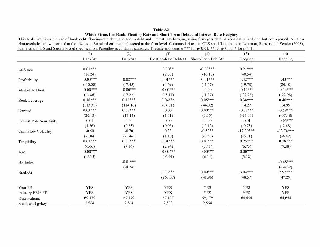
Table A2 Which Firms Use Bank, Floating-Rate and Short-Term Debt, and Interest Rate Hedging

This table examines the use of bank debt, floating-rate debt, short-term debt and interest rate hedging, using firm-year data. A constant is included but not reported. All firm characteristics are winsorized at the 1% level. Standard errors are clustered at the firm level. Columns 1-4 use an OLS specification, as in Lemmon, Roberts and Zender (2008), while columns 5 and 6 use a Probit specification. Parentheses contain t-statistics. The asterisks denote *** for p<0.01, ** for p<0.05, * for p<0.1.

(1) (2) (3) (4) (5) (6) Bank/At Bank/At Floating-Rate Debt/At Short-Term Debt/At Hedging Hedging

LnAssets 0.01*** 0.00** -0.00*** 0.21***

(16.24) (2.55) (-10.13) (40.54)

Profitability -0.03*** -0.02*** 0.01*** -0.01*** 1.42*** 1.43*** (-10.08) (-7.45) (4.69) (-4.67) (19.78) (20.10)

Market to Book -0.00*** -0.00*** -0.00*** -0.00 -0.14*** -0.14*** (-3.86) (-7.22) (-3.11) (-1.27) (-22.25) (-22.98)

Book Leverage 0.18*** 0.18*** 0.04*** 0.05*** 0.38*** 0.40*** (113.33) (114.16) (34.31) (44.82) (14.27) (14.99)

Unrated 0.03*** 0.03*** 0.00 0.00*** -0.37*** -0.58*** (20.13) (17.13) (1.31) (3.35) (-21.33) (-37.48)

Interest Rate Sensitivity 0.01 0.00 0.00 -0.00 -0.01 -0.05*** (1.56) (0.83) (0.05) (-0.12) (-0.73) (-2.68)

Cash Flow Volatility -0.50 -0.70 0.33 -0.52** -12.79*** -13.74*** (-1.04) (-1.46) (1.10) (-2.33) (-6.31) (-6.82)

Tangibility 0.03*** 0.03*** 0.01*** 0.01*** 0.25*** 0.28*** (6.66) (7.16) (2.94) (3.71) (6.73) (7.58)

Age -0.00*** -0.00*** 0.00*** 0.00*** (-5.35) (-6.44) (6.14) (3.18)

HP Index -0.01*** -0.48*** (-4.78) (-34.32)

Bank/At 0.76*** 0.09*** 3.04*** 2.92*** (268.07) (41.96) (48.57) (47.29)

Year FE YES YES YES YES YES YES Industry FF48 FE YES YES YES YES YES YES

Observations 69,179 69,179 67,127 69,179 64,654 64,654

Number of gvkey 2,564 2,564 2,503 2,564

 

 

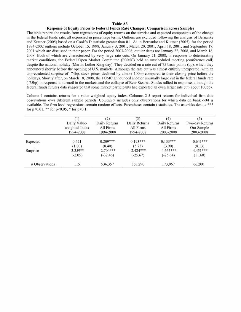
Table A3

Response of Equity Prices to Federal Funds Rate Changes: Comparison across Samples The table reports the results from regressions of equity returns on the surprise and expected components of the change in the federal funds rate, all expressed in percentage terms. Outliers are excluded following the analysis of Bernanke and Kuttner (2005) based on a Cook’s D statistic greater than 0.1. As in Bernanke and Kuttner (2005), for the period 1994-2002 outliers include October 15, 1998, January 3, 2001, March 20, 2001, April 18, 2001, and September 17, 2001 which are discussed in their paper. For the period 2003-2008, outlier dates are January 22, 2008, and March 18, 2008. Both of which are characterized by very large rate cuts. On January 21, 2008, in response to deteriorating market conditions, the Federal Open Market Committee (FOMC) held an unscheduled meeting (conference call) despite the national holiday (Martin Luther King day). They decided on a rate cut of 75 basis points (bp), which they announced shortly before the opening of U.S. markets. Although the rate cut was almost entirely unexpected, with an unprecedented surprise of -74bp, stock prices declined by almost 100bp compared to their closing price before the holidays. Shortly after, on March 18, 2008, the FOMC announced another unusually large cut in the federal funds rate (-75bp) in response to turmoil in the markets and the collapse of Bear Stearns. Stocks rallied in response, although the federal funds futures data suggested that some market participants had expected an even larger rate cut (about 100bp).

Column 1 contains returns for a value-weighted equity index. Columns 2-5 report returns for individual firm-date observations over different sample periods. Column 5 includes only observations for which data on bank debt is available. The firm level regressions contain random effects. Parentheses contain t-statistics. The asterisks denote *** for p<0.01, ** for p<0.05, * for p<0.1.

(1) (2) (3) (4) (5) Daily Value-

weighted Index 1994-2008

Daily Returns All Firms 1994-2008

Daily Returns All Firms 1994-2002

Daily Returns All Firms 2003-2008

Two-day Returns Our Sample 2003-2008

Expected 0.421 0.209*** 0.193*** 0.133*** -0.641*** (1.00) (8.40) (5.73) (3.90) (8.13) Surprise -3.359** -2.704*** -2.424*** -4.665*** -4.451*** (-2.05) (-32.46) (-25.67) (-25.64) (11.60)

# Observations 115 536,357 363,290 173,067 66,200

 

 

Table A4 The Role of Bank Debt Usage and Interest Rate Risk Exposure in the Transmission of Monetary Policy

This table examines how the reaction of firm equity prices to surprise changes in the federal funds rate varies with their level of bank dependence. The sample consists of U.S. firms covered by Capital IQ, CRSP and Compustat from 2003 to 2008, excluding utilities (SIC 4900-4949) and financials (SIC 6000-6999). We focus on firms with December fiscal year end to avoid asynchronous balance sheet items and use 2-day returns in order to allow the effect of bank-debt to be fully incorporated in stock prices. We remove firm-year observations with negative revenues, missing information on total assets, or a value of total assets under 10 million. We also discard penny stocks, defined as those with a price of less than $5. The sample comprises 43 monetary policy events from 2003 to 2008. Firm characteristics are demeaned and are lagged by one year and winsorized at the 1% level. The regression specification is as in equation (1). Unreported terms include a constant and non-interacted coefficients. In specification (6) we add undrawn credit lines to bank debt and normalize the resulting ratio to have the same standard deviation as the original BankDebt/At. Standard errors are clustered at the date level in specifications (1)-(2) and two-way clustered at the date and industry levels in specifications (4)-(7). Industries are Fama-French 48 industries. Square brackets around the estimates of the coefficient of surprise in columns (4)-(7) are introduced to indicate that, due to the interaction of surprise with industry fixed effects, these estimates cannot be interpreted as the estimate applicable to the average firm. Parentheses contain t-statistics. The asterisks denote *** for p<0.01, ** for p<0.05, * for p<0.1. Hadlock and Pierce (2010) measure given by HP = -0.548*Size+0.025*Size2-0.031*Age.

(1) (2a) (2b) (2c) (3) (4) (5) (6) (7) (8) (9)

No Controls

Mkt. Return Control

CAPM Control

Fama-FrenchControl

Other Controls

Industry FE & Event-Industry

Clustering

Inc. Undrawn Credit Lines

Other Controls

Firm Fixed Effects

Instrumental Variable

Floating Rate Debt

Surprise -4.97*** 2.93*** 1.28*** -0.09 -8.02*** [-7.44] [-8.07] [-9.83] -8.04*** -8.07*** -8.81***

(-13.03) (8.22) (3.66) (-0.25) (-17.72) (-0.83) (-0.90) (-1.10) (-3.33) (-17.12) (-3.63)

Surprise*(BankDebt/At) -14.10*** -12.31*** -10.52*** -8.09*** -16.34*** -16.77*** -14.62*** -15.22*** -16.37*** -14.50 -13.79**

(-4.35) (-4.15) (-3.54) (-2.63) (-4.17) (-3.82) (-3.10) (-3.30) (-2.69) (-0.58) (-2.48)

Surprise*LnAssets -0.95*** -1.12*** -1.06*** -0.07 -0.94*** -1.00** -1.01**

(-3.67) (-4.19) (-3.99) (-0.15) (-2.64) (-2.06) (-2.53)

Surprise*Book Leverage 3.28** 3.83* 2.59 4.24** 3.15 2.44 4.49*

(1.96) (1.85) (1.32) (1.98) (1.28) (0.40) (1.71)

Surprise*Profitability -16.10*** -11.49** -11.08** -8.16 -15.36** -15.68*** -16.54

(-6.10) (-2.19) (-2.13) (-1.33) (-2.08) (-4.06) (-1.45)

Surprise*M/B -0.02 -0.41 -0.41 -0.71 0.01 0.10 0.43

(-0.08) (-0.77) (-0.78) (-1.31) (0.01) (0.25) (0.42)

Surprise*Int Rate Sensitivity -7.05**

(-2.24)

Surprise*Cash-Flow Volatility -77.57

(-0.55)

Surprise*Beta 1.47**

(2.16)

Surprise*Cash Holdings 3.37

(0.96)

Surprise*HP 4.22***

(3.42)

Firm FE NO NO NO NO NO NO NO NO YES YES YES

FF48 Industry FE NO NO NO NO NO YES YES YES NO NO NO

Year FE NO NO NO NO YES YES YES YES YES YES YES

Surprise*FF48 Industry FE NO NO NO NO NO YES YES YES NO NO NO

Cluster (Fed event*IndustryFF48) NO NO NO NO NO YES YES YES YES NO YES

Observations 64,682 64,682 64,557 64,549 64,428 62,871 62,746 55,506 64,428 63,626 41,710

 

 

Table A5 The Role of Bank Debt Usage and Interest Rate Risk Exposure in the Transmission of Monetary Policy: Excluding Positive Rate Changes

This table repeats Table II after discarding those FOMC announcements with positive rate changes. Hedgers are defined on a yearly basis as those firms that report having hedged their interest rate risk from floating to fixed in their 10-K annual reports. Only firms with floating rate debt constituting more than 1% of total assets are included. Bank Debt/At is defined as bank debt (term loans plus drawn revolving credit) over the book value of assets (At). FloatingRateDebt /At is defined as floating rate debt over the book value of assets (At). All regressions also include an unreported constant term, as well as ln(assets), book leverage, profitability, market-to-book, interest rate sensitivity, and their interaction with surprise. All firm characteristics are lagged by one year and winsorized at 1%. Parentheses contain t-statistics. The asterisks denote *** for p<0.01, ** for p<0.05, * for p<0.1. (1) (2) (3) (4) (5) (6) (7) (8)

Main Variables Non-

Hedgers Hedgers Non-

Hedgers Hedgers Non-

Hedgers Hedgers Non-

Hedgers Hedgers

Surprise -3.44*** -7.84*** -4.42 -5.96* -3.94*** -7.41*** -5.14* -5.41* (-3.28) (-7.71) (-1.62) (-1.94) (-3.92) (-7.56) (-1.91) (-1.74)

Surprise *(BankDebt/At) -25.20*** 0.59 -38.68*** 1.96 (-2.91) (0.10) (-3.13) (0.20)

Surprise *(FloatingRateDebt /At) -20.64** -3.98 -29.97** -6.35

(-2.47) (-0.73) (-2.26) (-0.64) 25.61**

(2.48) 40.64***

(2.75) 16.32* (1.66)

23.62 (1.43)

Surprise *log(Assets) -2.02*** -0.70 -1.65** -0.98 (-2.82) (-0.97) (-2.26) (-1.37) Surprise *Book Leverage 6.43 -6.13 6.02 -3.62 (1.29) (-1.32) (1.16) (-0.78) Surprise *Market-to-Book -0.25 2.34* -0.16 2.35* (-0.19) (1.66) (-0.12) (1.67) Surprise *Profitability -13.14 -24.14 -13.79 -24.12 (-1.07) (-1.07) (-1.13) (-1.06) Surprise *Int. Rate Sensitivity -9.80* -5.33 -10.38* -5.57 (-1.67) (-0.80) (-1.79) (-0.84)

Firm Controls NO NO YES YES NO NO YES YES

Firm FE NO NO YES YES NO NO YES YES

Surprise*Firm Controls NO NO YES YES NO NO YES YES

Cluster (Fed event*IndustryFF48) NO NO YES YES NO NO YES YES

Observations 7,067 7,585 7,067 7,585 7,067 7,585 7,067 7,585

 

 

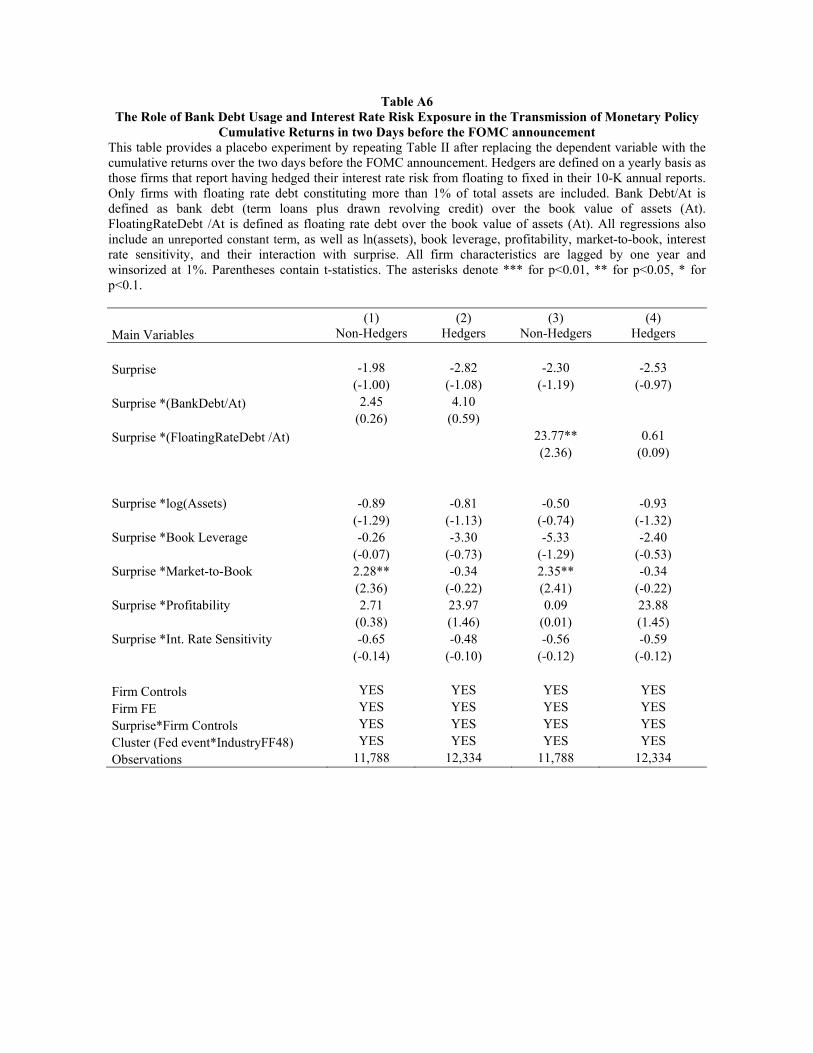
Table A6 The Role of Bank Debt Usage and Interest Rate Risk Exposure in the Transmission of Monetary Policy

Cumulative Returns in two Days before the FOMC announcement This table provides a placebo experiment by repeating Table II after replacing the dependent variable with the cumulative returns over the two days before the FOMC announcement. Hedgers are defined on a yearly basis as those firms that report having hedged their interest rate risk from floating to fixed in their 10-K annual reports. Only firms with floating rate debt constituting more than 1% of total assets are included. Bank Debt/At is defined as bank debt (term loans plus drawn revolving credit) over the book value of assets (At). FloatingRateDebt /At is defined as floating rate debt over the book value of assets (At). All regressions also include an unreported constant term, as well as ln(assets), book leverage, profitability, market-to-book, interest rate sensitivity, and their interaction with surprise. All firm characteristics are lagged by one year and winsorized at 1%. Parentheses contain t-statistics. The asterisks denote *** for p<0.01, ** for p<0.05, * for p<0.1. (1) (2) (3) (4) Main Variables Non-Hedgers Hedgers Non-Hedgers Hedgers

Surprise -1.98 -2.82 -2.30 -2.53 (-1.00) (-1.08) (-1.19) (-0.97)

Surprise *(BankDebt/At) 2.45 4.10 (0.26) (0.59)

Surprise *(FloatingRateDebt /At) 23.77** 0.61

(2.36) (0.09) Surprise *log(Assets) -0.89 -0.81 -0.50 -0.93 (-1.29) (-1.13) (-0.74) (-1.32) Surprise *Book Leverage -0.26 -3.30 -5.33 -2.40 (-0.07) (-0.73) (-1.29) (-0.53) Surprise *Market-to-Book 2.28** -0.34 2.35** -0.34 (2.36) (-0.22) (2.41) (-0.22) Surprise *Profitability 2.71 23.97 0.09 23.88 (0.38) (1.46) (0.01) (1.45) Surprise *Int. Rate Sensitivity -0.65 -0.48 -0.56 -0.59 (-0.14) (-0.10) (-0.12) (-0.12)

Firm Controls YES YES YES YES

Firm FE YES YES YES YES

Surprise*Firm Controls YES YES YES YES

Cluster (Fed event*IndustryFF48) YES YES YES YES

Observations 11,788 12,334 11,788 12,334

 

 

Table A7 The Role of Interest Rate Risk Exposure in the Transmission of Monetary Policy:

First Stage Regressions of Instrumental Variables Analysis Following Graham and Smith (1999) and Campello, Lin, Ma, Zou (2011), Vol is the volatility of taxable income, Corr is the serial correlation of taxable income, DITC is a dummy for investment tax credits, DNOL is a dummy for net operating losses, and DSmallNeg (DSmallPos) is a dummy for small negative (positive) taxable income. We calculate the volatility of taxable income and the serial correlation of taxable income on a rolling basis, using historical annual data up to the year of interest, starting in 1989. Column (1) uses lagged hedging dummy as instrument for hedging. Column (2) uses the variables underlying the convexity measure, excluding Vol, whereas column (3) uses all variables. Column (4) uses the tax convexity measure, Convexity, directly, as given in the text. Column (5) uses both the lagged hedging dummy and the tax convexity measure. Only firms with floating rate debt constituting more than 1% of total assets are included. A constant, non-interacted terms, and the policy surprise interacted with firm size, book leverage, profitability and the market-to-book ratio are included but not reported for brevity. All firm characteristics are lagged by one year and winsorized at 1%. Parentheses contain t-statistics. The asterisks denote *** for p<0.01, ** for p<0.05, * for p<0.1.

Panel A: Bank Debt

(1) (2) (3) (4) (5) IV IV1 IV2 IV3 IV VARIABLES Surprise*(BankDebt/At)*

L.hedging Convexity Convexity Convexity Both

L.hedgingdummy 0.69*** 0.67*** (116.06) (73.74) Corr -0.01 -0.00 (-0.71) (-0.31) DITC -0.23*** -0.23*** (-12.08) (-11.74) DSmallNeg -0.87 -0.74 (-0.42) (-0.36) DNOL 0.16*** 0.16*** (11.48) (11.58) DNOL*DSmallNeg 2.17 1.77 (0.67) (0.55) DSmallPos 1.41 1.59 (0.03) (0.04) DNOL*DSmallPos -2.00 -2.28 (-0.05) (-0.05) Vol -0.00 (-0.40) Convexity 0.02*** -0.00 (9.75) (-1.62) Observations 23,413 12,009 12,009 12,009 11,665 R-squared 0.86 0.75 0.75 0.74 0.87 Firm FE YES YES YES YES YES Firm Controls YES YES YES YES YES Surprise*Firm Controls YES YES YES YES YES F-stat 6012 441.5 385.0 1390 2024

 

 

Panel B: Floating Rate Debt

(1) (2) (3) (4) (5) IV IV1 IV2 IV3 IV VARIABLES Surprise*(FloatingRateDebt/At)*

L.hedging Convexity Convexity Convexity Both

L.hedgingdummy 0.70*** 0.68*** (120.40) (77.82) Corr -0.18*** -0.17*** (-12.35) (-11.99) DITC -0.16*** -0.15*** (-8.30) (-7.88) DSmallNeg 3.25 2.00 (0.49) (0.30) DNOL 0.15*** 0.15*** (10.89) (10.86) DNOL*DSmallNeg -2.78 -1.62 (-0.44) (-0.25) DSmallPos 8.68 8.31 (0.04) (0.04) DNOL*DSmallPos -9.37 -9.20 (-0.05) (-0.05) Vol 0.00 (0.57) Convexity 0.04*** 0.01*** (20.86) (8.36) Observations 23,413 12,009 12,009 12,009 11,665 R-squared 0.87 0.77 0.77 0.76 0.88 Firm FE YES YES YES YES YES Firm Controls YES YES YES YES YES Surprise*Firm Controls YES YES YES YES YES F-stat 6564 477.1 415.8 1553 2346

 

 

Table A8 Interest Rate Risk Exposure and the Transmission of Monetary Policy: The Role of Financing Constraints

Whited-Wu and Kaplan_Zingales Measures Hedgers are defined on a yearly basis as those firms that report having hedged their interest rate risk from floating to fixed in their 10-K annual reports. Financial constraints are proxied with Whited-Wu (WW) quarterly measure as reported in Whited and Wu (2006) and Kaplan-Zingales (KZ) measure, as reported in Lamont, Polk, Saa-Requejo (2001). Accordingly, KZ = –1.001909[(IB+DP)/lagged PPENT] + 0.2826389[ (AT + PRCC_F×CSHO - CEQ - TXDB)/AT] + 3.139193[(DLTT + DLC)/(DLTT + DLC + SEQ)] – 39.3678[(DVC + DVP)/lagged PPENT] – 1.314759[CHE/lagged PPENT] and WW = –0.091 [(IB + DP)/AT] – 0.062[indicator set to one if DVC + DVP is positive, and zero otherwise] + 0.021[DLTT/AT] – 0.044[log(AT)] + 0.102[average SIC 3-digit industry sales growth each year] – 0.035[sales growth]. All capitalized mnemonics refer to Compustat data items. The financial constraint measure takes value 1 if the corresponding measure is above the median in a given year. Only firms with floating rate debt constituting more than 1% of total assets are included. Bank Debt/At is defined as bank debt (term loans plus drawn revolving credit) over the book value of assets (At). All regressions also include an unreported constant term, as well as ln(assets), book leverage, profitability, market-to-book, interacted with surprise and uninteracted. All firm and lender characteristics are lagged by one year and winsorized at 1%. Parentheses contain t-statistics. The asterisks denote *** for p<0.01, ** for p<0.05, * for p<0.1.

(1) (2) (3) (4) (5) (6) (7) (8) LOW WW HIGH WW LOW WW HIGH WW LOW KZ HIGH KZ LOW KZ HIGH KZ VARIABLES NONHEDGER NONHEDGER HEDGER HEDGER NONHEDGER NONHEDGER HEDGER HEDGER Surprise -2.59 -6.66** -6.11** -11.56*** -6.86*** -3.51** -3.24 -7.86*** (-1.08) (-2.54) (-2.31) (-3.40) (-3.24) (-2.04) (-0.89) (-3.68) Surprise*BankDebt/At -18.82 -51.93*** 0.59 6.95 -45.70* -45.79*** -26.92* 7.91 (-1.24) (-3.36) (0.07) (0.47) (-1.84) (-3.76) (-1.72) (0.91)

Surpr.*(BankDebt/At)* Constrained

-33.11 (1.50)

6.36 (0.39)

-0.0834 (0.00)

34.83* (1.84)

Firm FE YES YES YES YES YES YES YES YES Firm Controls YES YES YES YES YES YES YES YES Surprise*Firm Controls YES YES YES YES YES YES YES YES Observations 5,291 5,996 7,893 3,795 3,879 6,909 2,703 8,436 R-squared 0.01 0.01 0.02 0.01 0.01 0.01 0.02 0.02 Number of gvkey 363 489 450 285 344 510 189 516

 

 

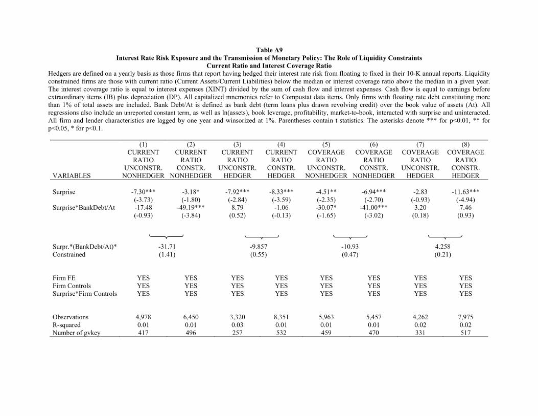
Table A9 Interest Rate Risk Exposure and the Transmission of Monetary Policy: The Role of Liquidity Constraints

Current Ratio and Interest Coverage Ratio Hedgers are defined on a yearly basis as those firms that report having hedged their interest rate risk from floating to fixed in their 10-K annual reports. Liquidity constrained firms are those with current ratio (Current Assets/Current Liabilities) below the median or interest coverage ratio above the median in a given year. The interest coverage ratio is equal to interest expenses (XINT) divided by the sum of cash flow and interest expenses. Cash flow is equal to earnings before extraordinary items (IB) plus depreciation (DP). All capitalized mnemonics refer to Compustat data items. Only firms with floating rate debt constituting more than 1% of total assets are included. Bank Debt/At is defined as bank debt (term loans plus drawn revolving credit) over the book value of assets (At). All regressions also include an unreported constant term, as well as ln(assets), book leverage, profitability, market-to-book, interacted with surprise and uninteracted. All firm and lender characteristics are lagged by one year and winsorized at 1%. Parentheses contain t-statistics. The asterisks denote *** for p<0.01, ** for p<0.05, * for p<0.1.

(1) (2) (3) (4) (5) (6) (7) (8) CURRENT

RATIO UNCONSTR.

CURRENT RATIO

CONSTR.

CURRENT RATIO

UNCONSTR.

CURRENT RATIO

CONSTR.

COVERAGE RATIO

UNCONSTR.

COVERAGE RATIO

CONSTR.

COVERAGE RATIO

UNCONSTR.

COVERAGE RATIO

CONSTR. VARIABLES NONHEDGER NONHEDGER HEDGER HEDGER NONHEDGER NONHEDGER HEDGER HEDGER Surprise -7.30*** -3.18* -7.92*** -8.33*** -4.51** -6.94*** -2.83 -11.63*** (-3.73) (-1.80) (-2.84) (-3.59) (-2.35) (-2.70) (-0.93) (-4.94) Surprise*BankDebt/At -17.48 -49.19*** 8.79 -1.06 -30.07* -41.00*** 3.20 7.46 (-0.93) (-3.84) (0.52) (-0.13) (-1.65) (-3.02) (0.18) (0.93)

Surpr.*(BankDebt/At)* Constrained

-31.71 (1.41)

-9.857 (0.55)

-10.93 (0.47)

4.258 (0.21)

Firm FE YES YES YES YES YES YES YES YES Firm Controls YES YES YES YES YES YES YES YES Surprise*Firm Controls YES YES YES YES YES YES YES YES Observations 4,978 6,450 3,320 8,351 5,963 5,457 4,262 7,975 R-squared 0.01 0.01 0.03 0.01 0.01 0.01 0.02 0.02 Number of gvkey 417 496 257 532 459 470 331 517

 

 

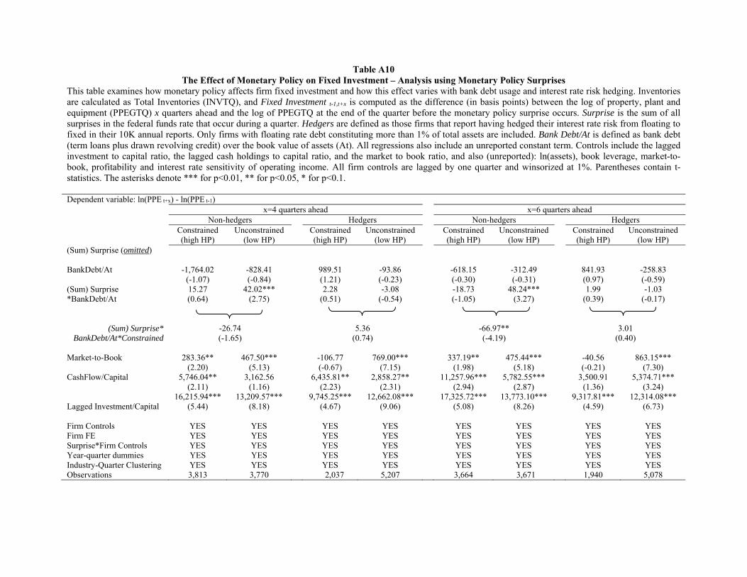
Table A10 The Effect of Monetary Policy on Fixed Investment – Analysis using Monetary Policy Surprises

This table examines how monetary policy affects firm fixed investment and how this effect varies with bank debt usage and interest rate risk hedging. Inventories are calculated as Total Inventories (INVTQ), and Fixed Investment t-1,t+x is computed as the difference (in basis points) between the log of property, plant and equipment (PPEGTQ) x quarters ahead and the log of PPEGTQ at the end of the quarter before the monetary policy surprise occurs. Surprise is the sum of all surprises in the federal funds rate that occur during a quarter. Hedgers are defined as those firms that report having hedged their interest rate risk from floating to fixed in their 10K annual reports. Only firms with floating rate debt constituting more than 1% of total assets are included. Bank Debt/At is defined as bank debt (term loans plus drawn revolving credit) over the book value of assets (At). All regressions also include an unreported constant term. Controls include the lagged investment to capital ratio, the lagged cash holdings to capital ratio, and the market to book ratio, and also (unreported): ln(assets), book leverage, market-to-book, profitability and interest rate sensitivity of operating income. All firm controls are lagged by one quarter and winsorized at 1%. Parentheses contain t-statistics. The asterisks denote *** for p<0.01, ** for p<0.05, * for p<0.1. Dependent variable: ln(PPE t+x) - ln(PPE t-1) x=4 quarters ahead x=6 quarters ahead Non-hedgers Hedgers Non-hedgers Hedgers Constrained

(high HP) Unconstrained

(low HP) Constrained

(high HP) Unconstrained

(low HP) Constrained

(high HP) Unconstrained

(low HP) Constrained

(high HP) Unconstrained

(low HP) (Sum) Surprise (omitted) BankDebt/At -1,764.02 -828.41 989.51 -93.86 -618.15 -312.49 841.93 -258.83 (-1.07) (-0.84) (1.21) (-0.23) (-0.30) (-0.31) (0.97) (-0.59) (Sum) Surprise *BankDebt/At

15.27 42.02*** 2.28 -3.08 -18.73 48.24*** 1.99 -1.03 (0.64) (2.75) (0.51) (-0.54) (-1.05) (3.27) (0.39) (-0.17)

(Sum) Surprise* BankDebt/At*Constrained

-26.74 5.36 -66.97** 3.01 (-1.65) (0.74) (-4.19) (0.40)

Market-to-Book 283.36** 467.50*** -106.77 769.00*** 337.19** 475.44*** -40.56 863.15*** (2.20) (5.13) (-0.67) (7.15) (1.98) (5.18) (-0.21) (7.30) CashFlow/Capital 5,746.04** 3,162.56 6,435.81** 2,858.27** 11,257.96*** 5,782.55*** 3,500.91 5,374.71*** (2.11) (1.16) (2.23) (2.31) (2.94) (2.87) (1.36) (3.24)

Lagged Investment/Capital 16,215.94*** 13,209.57*** 9,745.25*** 12,662.08*** 17,325.72*** 13,773.10*** 9,317.81*** 12,314.08***

(5.44) (8.18) (4.67) (9.06) (5.08) (8.26) (4.59) (6.73) Firm Controls YES YES YES YES YES YES YES YES Firm FE YES YES YES YES YES YES YES YES Surprise*Firm Controls YES YES YES YES YES YES YES YES Year-quarter dummies YES YES YES YES YES YES YES YES Industry-Quarter Clustering YES YES YES YES YES YES YES YES Observations 3,813 3,770 2,037 5,207 3,664 3,671 1,940 5,078

 

 

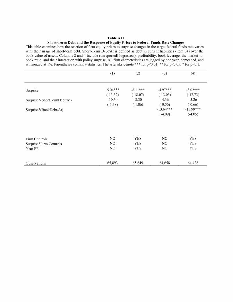
Table A11 Short-Term Debt and the Response of Equity Prices to Federal Funds Rate Changes

This table examines how the reaction of firm equity prices to surprise changes in the target federal funds rate varies with their usage of short-term debt. Short-Term Debt/At is defined as debt in current liabilities (item 34) over the book value of assets. Columns 2 and 4 include (unreported) log(assets), profitability, book leverage, the market-to-book ratio, and their interaction with policy surprise. All firm characteristics are lagged by one year, demeaned, and winsorized at 1%. Parentheses contain t-statistics. The asterisks denote *** for p<0.01, ** for p<0.05, * for p<0.1.

(1) (2) (3) (4)

Surprise -5.04*** -8.11*** -4.97*** -8.02*** (-13.32) (-18.07) (-13.03) (-17.73)

Surprise*(ShortTermDebt/At) -10.30 -8.30 -4.36 -5.26 (-1.38) (-1.06) (-0.56) (-0.66)

Surprise*(BankDebt/At) -13.64*** -15.99*** (-4.09) (-4.05)

Firm Controls NO YES NO YES

Surprise*Firm Controls NO YES NO YES

Year FE NO YES NO YES

Observations 65,893 65,649 64,658 64,428

 

 

Table A12 Is Bank Debt Special for the Transmission of Monetary Policy? Normalizing Bank Debt with Total Debt

This table examines how the reaction of firm equity prices to changes in the federal funds rate varies with their level of bank dependence. The sample consists of U.S. firms covered by Capital IQ, CRSP and Compustat from 2003 to 2008, excluding utilities (SIC 4900-4949) and financials (SIC 6000-6999). We focus on firms with December fiscal year end to avoid asynchronous balance sheet items and use 2-day returns in order to allow the effect of bank-debt to be fully incorporated in stock prices. We remove firm-year observations with negative revenues, missing information on total assets, or a value of total assets under 10 million. We also discard penny stocks, defined as those with a price of less than $5. The sample comprises 43 monetary policy events from 2003 to 2008. Firm characteristics are demeaned and are lagged by one year and winsorized at the 1% level. The regression specification is as in equation (1). Unreported terms include a constant and non-interacted coefficients. In specification (5) we add undrawn credit lines to bank debt and normalize the resulting ratio to have the same standard deviation as the original BankDebt/At. Standard errors are clustered at the date level in specifications (1)-(2) and two-way clustered at the date and industry levels in specifications (4)-(7). Industries are Fama-French 48 industries. Parentheses contain t-statistics. The asterisks denote *** for p<0.01, ** for p<0.05, * for p<0.1.

(1) (2) (3) (4) (5) (6) (7) (8)

No Controls

With Controls Event-indust. Clustering

Including Credit Lines

Other Controls

Firm Fixed Effects

Instrumental Variable

Floating Rate Debt

Surprise -5.60*** -8.20*** [-8.27] [-8.58] [-10.51] -8.19*** -8.22*** -8.57***

(-13.65) (-16.33) (-0.92) (-0.96) (-1.17) (-3.51) (-14.32) (-3.51)

Surprise*(BankDebt/Debt) -2.18** -3.04*** -3.06*** -1.61 -3.14*** -2.85** -3.20 -1.53

(-2.12) (-2.73) (-2.87) (-1.58) (-2.75) (-2.18) (-0.35) (-0.95)

Surprise*LnAssets -0.77*** -1.05*** -0.79*** -0.15 -0.73* -0.79 -0.85**

(-2.76) (-3.74) (-2.83) (-0.32) (-1.90) (-0.86) (-2.16)

Surprise*Book Leverage 0.38 0.52 -0.05 0.80 0.30 0.52 1.32

(0.25) (0.28) (-0.02) (0.40) (0.13) (0.32) (0.50)

Surprise*Profitability -21.36*** -14.62** -15.21** -12.29 -21.73** -22.41*** -17.99

(-6.93) (-2.26) (-2.35) (-1.53) (-2.40) (-4.53) (-1.58)

Surprise*M/B 0.40 -0.16 -0.02 -0.23 0.45 0.40 0.55

(1.20) (-0.25) (-0.04) (-0.33) (0.57) (0.75) (0.55)

Surprise*Int Rate Sensitivity -7.42**

(-2.44)

Surprise*Cash-Flow Volatility -91.93

(-0.62)

Surprise*Beta 1.83**

(2.44)

Surprise*Cash Holdings 1.19

(0.32)

Surprise*HP 3.94***

(3.13)

Firm FE NO NO NO NO NO YES YES YES

FF48 Industry FE NO NO YES YES YES NO NO NO

Year FE NO YES YES YES YES YES YES YES

Interacted FF48 Industry FE NO NO YES YES YES NO NO NO

Cluster (Fed event*IndustryFF48) NO NO YES YES YES YES NO YES

Observations 53,054 53,028 51,963 51,963 45,972 53,028 52,398 41,665

 

 

Table A13 Bank Debt Specialness and Firm Financing Constraints

This table examines how the effect of monetary policy on firm stock prices varies with their exposure to bank debt and their level of financial constraints. Financial constraints are proxied with the firm’s age and the Hadlock and Pierce (2010) measure given by HP = -0.548*Size+0.025*Size2-0.031*Age. Firm size is defined to be the log of assets (inflation adjusted to 2004). Age is defined as the current year minus the first year that the firm has a non-missing stock price in CRSP. Firm size and age are at the 1% tails on the low end, and at the $4.5 billion and thirty-seven year points on the high end. The financial constraint measure takes value 1 if the firm’s age is below the median or firm’s HP statistic is above the median in a given year. Only firms with floating rate debt constituting more than 1% of total assets are included. A constant, non-interacted terms, and the policy surprise interacted with firm size book leverage, profitability and the market-to-book ratio are included but not reported. All firm characteristics are lagged by one year and winsorized at the 1% level. Industries are defined according to the Fama French 48 sector grouping. Parentheses contain t-statistics. The asterisks denote *** for p<0.01, ** for p<0.05, * for p<0.1. (1) (2) (3) (4) VARIABLES AGE HP AGE HP Surprise -4.92*** -2.31 -5.47*** -2.80 (-3.25) (-1.18) (-3.69) (-1.47) Surprise*Financial Constraint Measure 0.67 -3.85 0.56 -4.28* (0.36) (-1.57) (0.31) (-1.79) Surprise*Hedging -1.95 -0.83 -1.29 (-0.95) (-0.42) (-0.63) Surprise*(BankDebt/At) -28.00** -29.20** (-2.50) (-2.46) Surprise*(BankDebt/At)*Financial Constraint Measure -16.79 -12.50 (-1.43) (-1.04) Surprise*(BankDebt/At)*Hedging 41.25*** 40.41*** (3.36) (3.27) Surprise*(FloatingRateDebt /At) -19.31* -25.18** (-1.73) (-2.21) Surprise*(FloatingRateDebt /At)*Financial Constraint Measure -17.02 -5.33 (-1.48) (-0.45) Surprise*(FloatingRateDebt /At)*Hedging 24.55** 26.06** (2.04) (2.16) Firm FE YES YES YES YES Firm Controls YES YES YES YES Surprise*Firm Controls YES YES YES YES Observations 24,123 24,123 24,123 24,123 R-squared 0.01 0.01 0.01 0.01 Number of gvkey 1,283 1,283 1,283 1,283

 

 

Table A14 – Dynamic Model Simulated Regressions: Variable Definitions

 

 

Table A15 The Effect of Monetary Policy using Simulated Data – Robustness using Bank Debt over Assets

This table displays regression results using simulated data from our dynamic model in Section 2.2 in which we use floating rate debt over total assets as our proxy for exposure to floating rate debt. It provides robustness for all the results on Tables II and II. Δrate refers to Surprise in stock return regressions, and Change in all other regressions. The definitions of all the variables used are described in detail in Appendix B. Parentheses contain t-statistics. The asterisks denote *** for p<0.01, ** for p<0.05, * for p<0.1.

Dep variable: Stock Returns

Stock Returns

Investment/K (4Q Ahead)

Investment/K (6Q Ahead)

Covenant Violation

Likelihood

Costs of Financial Distress

Interest Rate Coverage

Ratio (1) (2) (3) (4) (5) (6) (7) Δrate -14.52*** -11.60*** -1.81*** -0.99*** -0.21 -0.53*** -1.24*** (-49.05) (-54.70) (-48.09) (-25.52) (-0.88) (-9.38) (-4.53) Δrate *(BankDebt/At) -1.46*** -1.38*** -0.09*** -0.06*** 0.02 0.09*** 0.79*** (-60.03) (-79.83) (-31.87) (-21.18) (1.01) (19.58) (35.15) Constrained* Δrate *(BankDebt/At) -0.25*** -0.22*** -0.02** -0.01 -0.02 0.21*** 0.52***

(-3.95) (-4.93) (-2.32) (-0.35) (-0.40) (17.76) (8.99) Controls YES YES YES YES YES YES YES R-squared 0.72 0.24 0.19 0.07 0.56 0.55 0.48 Observations 38,000 38,000 38,000 38,000 38,000 38,000 38,000