at SciVerse ScienceDirect

Journal of Environmental Radioactivity 112 (2012) 155e159

Contents lists available

Journal of Environmental Radioactivity

journal homepage: www.elsevier .com/locate/ jenvrad

The total release of xenon-133 from the Fukushima Dai-ichi nuclear powerplant accident

Andreas Stohl a,*, Petra Seibert b, Gerhard Wotawa c

aNILU (Norwegian Institute for Air Research), Instituttveien 18, 2027 Kjeller, Norwayb Institute of Meteorology, University of Natural Resources and Life Sciences, Peter-Jordan-Str. 82, 1190 Vienna, AustriacCentral Institute for Meteorology and Geodynamics, Hohe Warte 38, 1190 Vienna, Austria

a r t i c l e i n f o

Article history:Received 12 April 2012Received in revised form25 May 2012Accepted 4 June 2012Available online 7 July 2012

Keywords:Nuclear accidentFukushimaXenon-133

* Corresponding author.E-mail addresses: Andreas.Stohl@nilu.no, ast@nilu

boku.ac.at (P. Seibert), gerhard.wotawa@zamg.ac.at (G

0265-931X/$ e see front matter � 2012 Elsevier Ltd.http://dx.doi.org/10.1016/j.jenvrad.2012.06.001

a b s t r a c t

The accident at the Fukushima Dai-ichi nuclear power plant (FD-NPP) on 11 March 2011 released largeamounts of radioactivity into the atmosphere. We determine the total emission of the noble gas xenon-133 (133Xe) using global atmospheric concentration measurements. For estimating the emissions, weused three different methods: (i) using a purely observation-based multi-box model, (ii) comparisons ofdispersion model results driven with GFS meteorological data with the observation data, and (iii) suchcomparisons with the dispersion model driven by ECMWF data. From these three methods, we haveobtained total 133Xe releases from FD-NPP of (i) 16.7 � 1.9 EBq, (ii) 14.2 � 0.8 EBq, and (iii) 19.0 � 3.4 EBq,respectively. These values are substantially larger than the entire 133Xe inventory of FD-NPP of about12.2 EBq derived from calculations of nuclear fuel burn-up. Complete release of the entire 133Xeinventory of FD-NPP and additional release of 133Xe due to the decay of iodine-133 (133I), which can addanother 2 EBq to the 133Xe FD-NPP inventory, is required to explain the atmospheric observations. Two ofour three methods indicate even higher emissions, but this may not be a robust finding given thedifferences between our estimates.

� 2012 Elsevier Ltd. All rights reserved.

1. Introduction

On 11 March 2011, an extraordinary magnitude 9.0 earthquakeoccurred about 130 km off the Pacific coast of Japan’s main islandHonshu, followed by a large tsunami (USGS, 2011). One of theconsequences was a station blackout at the Fukushima Dai-ichinuclear power plant (FD-NPP), which developed into a disasterleaving four of the six FD-NPP units heavily damaged. The resultwas a massive discharge of radionuclides. In the atmosphere, theradionuclides were transported throughout the Northern Hemi-sphere (Stohl et al., 2012) and could be detected at many stations(e.g. Bowyer et al., 2011).

The total amount of radioactivity released into the atmosphereis still uncertain. It can be estimated based on calculations of theradionuclide content of the nuclear reactors combined with acci-dent simulations, or using ambient atmospheric monitoring datatogether with some sort of inverse modelling. Japanese authorities

.no (A. Stohl), petra.seibert@. Wotawa).

All rights reserved.

used both approaches and provided estimates for many radionu-clides (NERH, 2011).

Of all the radionuclide emissions, the radioactive noble gasreleases can be quantified most accurately, since it is almost certainthat the entire noble gas inventory of the heavily damaged reactorunits 1e3 was set free into the atmosphere. For other radionuclides,only a small but highly uncertain fraction of the inventory wasreleased into the environment. Complete noble gas release was alsoassumed by the Japanese authorities (NERH, 2011) who estimateda release of 12.2 EBq of 133Xe, the most important radioactive noblegas with a half-life of 5.25 d. The inventory estimates of Bowyeret al. (2011) of 12 EBq 133Xe and Stohl et al. (2012) of 12.4 EBq133Xe are nearly identical. While the excellent agreement mayindicate that the inventory is known with high accuracy, the esti-mates are all based on similar methods, so the true uncertainty ofthe 133Xe inventory may be higher. Nevertheless, the 133Xe inven-tory should be known to within a few percent at most. However,using measured atmospheric concentrations at many stations inthe Northern Hemisphere (NH) together with inverse modelling,Stohl et al. (2011) obtained a much higher release of 16.7(13.4e20.0) EBq 133Xe. In a revision of their discussion paper, moreaccurate decay corrections for the measurement data resulted ina reduced estimate of 15.3 (12.2e18.3) EBq 133Xe (Stohl et al., 2012),

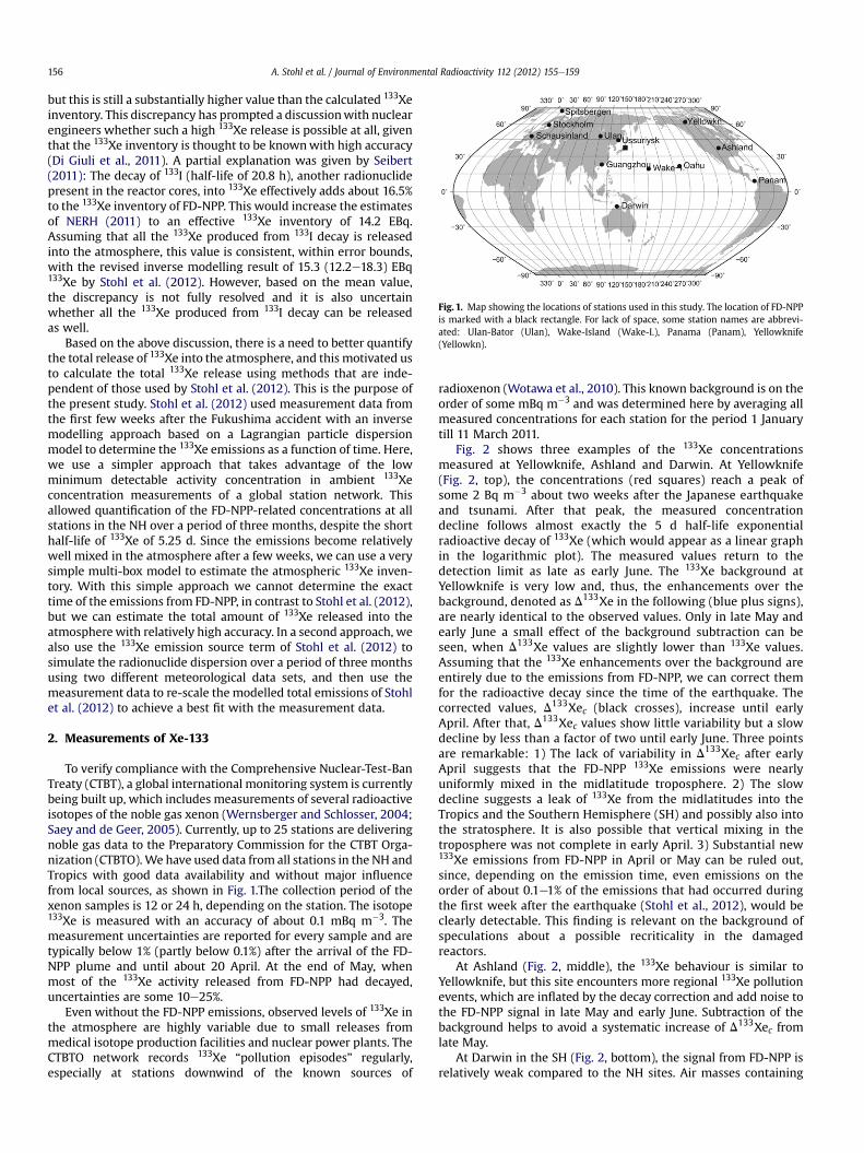
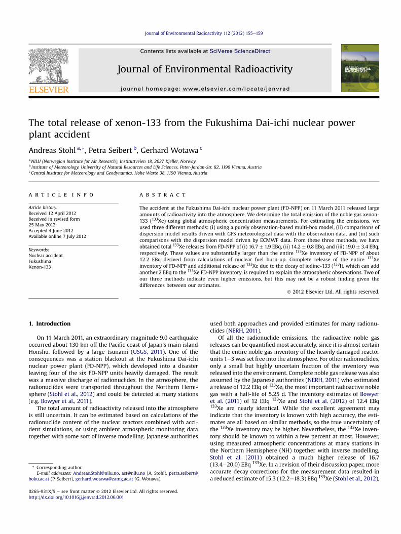
Fig. 1. Map showing the locations of stations used in this study. The location of FD-NPPis marked with a black rectangle. For lack of space, some station names are abbrevi-ated: Ulan-Bator (Ulan), Wake-Island (Wake-I.), Panama (Panam), Yellowknife(Yellowkn).

A. Stohl et al. / Journal of Environmental Radioactivity 112 (2012) 155e159156

but this is still a substantially higher value than the calculated 133Xeinventory. This discrepancy has prompted a discussionwith nuclearengineers whether such a high 133Xe release is possible at all, giventhat the 133Xe inventory is thought to be knownwith high accuracy(Di Giuli et al., 2011). A partial explanation was given by Seibert(2011): The decay of 133I (half-life of 20.8 h), another radionuclidepresent in the reactor cores, into 133Xe effectively adds about 16.5%to the 133Xe inventory of FD-NPP. This would increase the estimatesof NERH (2011) to an effective 133Xe inventory of 14.2 EBq.Assuming that all the 133Xe produced from 133I decay is releasedinto the atmosphere, this value is consistent, within error bounds,with the revised inverse modelling result of 15.3 (12.2e18.3) EBq133Xe by Stohl et al. (2012). However, based on the mean value,the discrepancy is not fully resolved and it is also uncertainwhether all the 133Xe produced from 133I decay can be releasedas well.

Based on the above discussion, there is a need to better quantifythe total release of 133Xe into the atmosphere, and this motivated usto calculate the total 133Xe release using methods that are inde-pendent of those used by Stohl et al. (2012). This is the purpose ofthe present study. Stohl et al. (2012) used measurement data fromthe first few weeks after the Fukushima accident with an inversemodelling approach based on a Lagrangian particle dispersionmodel to determine the 133Xe emissions as a function of time. Here,we use a simpler approach that takes advantage of the lowminimum detectable activity concentration in ambient 133Xeconcentration measurements of a global station network. Thisallowed quantification of the FD-NPP-related concentrations at allstations in the NH over a period of three months, despite the shorthalf-life of 133Xe of 5.25 d. Since the emissions become relativelywell mixed in the atmosphere after a few weeks, we can use a verysimple multi-box model to estimate the atmospheric 133Xe inven-tory. With this simple approach we cannot determine the exacttime of the emissions from FD-NPP, in contrast to Stohl et al. (2012),but we can estimate the total amount of 133Xe released into theatmosphere with relatively high accuracy. In a second approach, wealso use the 133Xe emission source term of Stohl et al. (2012) tosimulate the radionuclide dispersion over a period of three monthsusing two different meteorological data sets, and then use themeasurement data to re-scale the modelled total emissions of Stohlet al. (2012) to achieve a best fit with the measurement data.

2. Measurements of Xe-133

To verify compliance with the Comprehensive Nuclear-Test-BanTreaty (CTBT), a global international monitoring system is currentlybeing built up, which includes measurements of several radioactiveisotopes of the noble gas xenon (Wernsberger and Schlosser, 2004;Saey and de Geer, 2005). Currently, up to 25 stations are deliveringnoble gas data to the Preparatory Commission for the CTBT Orga-nization (CTBTO).We have used data from all stations in the NH andTropics with good data availability and without major influencefrom local sources, as shown in Fig. 1.The collection period of thexenon samples is 12 or 24 h, depending on the station. The isotope133Xe is measured with an accuracy of about 0.1 mBq m�3. Themeasurement uncertainties are reported for every sample and aretypically below 1% (partly below 0.1%) after the arrival of the FD-NPP plume and until about 20 April. At the end of May, whenmost of the 133Xe activity released from FD-NPP had decayed,uncertainties are some 10e25%.

Even without the FD-NPP emissions, observed levels of 133Xe inthe atmosphere are highly variable due to small releases frommedical isotope production facilities and nuclear power plants. TheCTBTO network records 133Xe “pollution episodes” regularly,especially at stations downwind of the known sources of

radioxenon (Wotawa et al., 2010). This known background is on theorder of some mBq m�3 and was determined here by averaging allmeasured concentrations for each station for the period 1 Januarytill 11 March 2011.

Fig. 2 shows three examples of the 133Xe concentrationsmeasured at Yellowknife, Ashland and Darwin. At Yellowknife(Fig. 2, top), the concentrations (red squares) reach a peak ofsome 2 Bq m�3 about two weeks after the Japanese earthquakeand tsunami. After that peak, the measured concentrationdecline follows almost exactly the 5 d half-life exponentialradioactive decay of 133Xe (which would appear as a linear graphin the logarithmic plot). The measured values return to thedetection limit as late as early June. The 133Xe background atYellowknife is very low and, thus, the enhancements over thebackground, denoted as D133Xe in the following (blue plus signs),are nearly identical to the observed values. Only in late May andearly June a small effect of the background subtraction can beseen, when D133Xe values are slightly lower than 133Xe values.Assuming that the 133Xe enhancements over the background areentirely due to the emissions from FD-NPP, we can correct themfor the radioactive decay since the time of the earthquake. Thecorrected values, D133Xec (black crosses), increase until earlyApril. After that, D133Xec values show little variability but a slowdecline by less than a factor of two until early June. Three pointsare remarkable: 1) The lack of variability in D133Xec after earlyApril suggests that the FD-NPP 133Xe emissions were nearlyuniformly mixed in the midlatitude troposphere. 2) The slowdecline suggests a leak of 133Xe from the midlatitudes into theTropics and the Southern Hemisphere (SH) and possibly also intothe stratosphere. It is also possible that vertical mixing in thetroposphere was not complete in early April. 3) Substantial new133Xe emissions from FD-NPP in April or May can be ruled out,since, depending on the emission time, even emissions on theorder of about 0.1e1% of the emissions that had occurred duringthe first week after the earthquake (Stohl et al., 2012), would beclearly detectable. This finding is relevant on the background ofspeculations about a possible recriticality in the damagedreactors.

At Ashland (Fig. 2, middle), the 133Xe behaviour is similar toYellowknife, but this site encounters more regional 133Xe pollutionevents, which are inflated by the decay correction and add noise tothe FD-NPP signal in late May and early June. Subtraction of thebackground helps to avoid a systematic increase of D133Xec fromlate May.

At Darwin in the SH (Fig. 2, bottom), the signal from FD-NPP isrelatively weak compared to the NH sites. Air masses containing

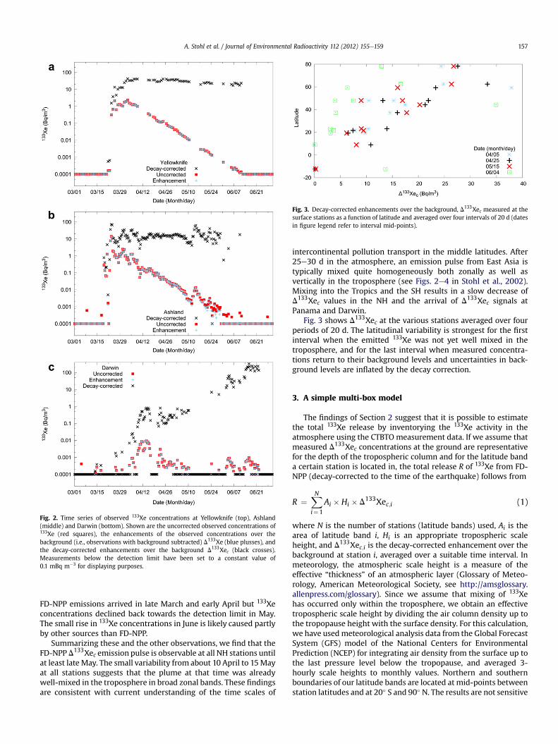
Fig. 3. Decay-corrected enhancements over the background, D133Xec measured at thesurface stations as a function of latitude and averaged over four intervals of 20 d (datesin figure legend refer to interval mid-points).

Fig. 2. Time series of observed 133Xe concentrations at Yellowknife (top), Ashland(middle) and Darwin (bottom). Shown are the uncorrected observed concentrations of133Xe (red squares), the enhancements of the observed concentrations over thebackground (i.e., observations with background subtracted) D133Xe (blue plusses), andthe decay-corrected enhancements over the background D133Xec (black crosses).Measurements below the detection limit have been set to a constant value of0.1 mBq m�3 for displaying purposes.

A. Stohl et al. / Journal of Environmental Radioactivity 112 (2012) 155e159 157

FD-NPP emissions arrived in late March and early April but 133Xeconcentrations declined back towards the detection limit in May.The small rise in 133Xe concentrations in June is likely caused partlyby other sources than FD-NPP.

Summarizing these and the other observations, we find that theFD-NPPD133Xec emission pulse is observable at all NH stations untilat least late May. The small variability from about 10 April to 15Mayat all stations suggests that the plume at that time was alreadywell-mixed in the troposphere in broad zonal bands. These findingsare consistent with current understanding of the time scales of

intercontinental pollution transport in the middle latitudes. After25e30 d in the atmosphere, an emission pulse from East Asia istypically mixed quite homogeneously both zonally as well asvertically in the troposphere (see Figs. 2e4 in Stohl et al., 2002).Mixing into the Tropics and the SH results in a slow decrease ofD133Xec values in the NH and the arrival of D133Xec signals atPanama and Darwin.

Fig. 3 shows D133Xec at the various stations averaged over fourperiods of 20 d. The latitudinal variability is strongest for the firstinterval when the emitted 133Xe was not yet well mixed in thetroposphere, and for the last interval when measured concentra-tions return to their background levels and uncertainties in back-ground levels are inflated by the decay correction.

3. A simple multi-box model

The findings of Section 2 suggest that it is possible to estimatethe total 133Xe release by inventorying the 133Xe activity in theatmosphere using the CTBTO measurement data. If we assume thatmeasured D133Xec concentrations at the ground are representativefor the depth of the tropospheric column and for the latitude banda certain station is located in, the total release R of 133Xe from FD-NPP (decay-corrected to the time of the earthquake) follows from

R ¼XN

i¼1

Ai � Hi � D133Xec;i (1)

where N is the number of stations (latitude bands) used, Ai is thearea of latitude band i, Hi is an appropriate tropospheric scaleheight, and D133Xec;i is the decay-corrected enhancement over thebackground at station i, averaged over a suitable time interval. Inmeteorology, the atmospheric scale height is a measure of theeffective “thickness” of an atmospheric layer (Glossary of Meteo-rology, American Meteorological Society, see http://amsglossary.allenpress.com/glossary). Since we assume that mixing of 133Xehas occurred only within the troposphere, we obtain an effectivetropospheric scale height by dividing the air column density up tothe tropopause height with the surface density. For this calculation,we have usedmeteorological analysis data from the Global ForecastSystem (GFS) model of the National Centers for EnvironmentalPrediction (NCEP) for integrating air density from the surface up tothe last pressure level below the tropopause, and averaged 3-hourly scale heights to monthly values. Northern and southernboundaries of our latitude bands are located at mid-points betweenstation latitudes and at 20� S and 90� N. The results are not sensitive

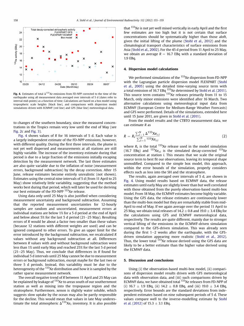
Fig. 4. Estimates of total D133Xe emissions from FD-NPP corrected to the time of theearthquake using all measurement data averaged over intervals of 5 d (dates refer tointerval mid-points) as a function of time. Calculations are based on a box model usingtropospheric scale heights (black line), and comparisons with dispersion modelsimulations driven with ECMWF (red line) and GFS (blue line) meteorological data.

A. Stohl et al. / Journal of Environmental Radioactivity 112 (2012) 155e159158

to changes of the southern boundary, since the measured concen-trations in the Tropics remain very low until the end of May (seeFig. 2c and Fig. 3).

Fig. 4 shows values of R for 16 intervals of 5 d. Each value isa largely independent estimate of the FD-NPP emissions, however,with different quality. During the first three intervals, the plume isnot yet well dispersed and measurements at all stations are stillhighly variable. The increase of the inventory estimate during thatperiod is due to a large fraction of the emissions initially escapingdetection by the measurement network. The last three estimatesare also quite variable due to the inflation of noise (measurementerrors, background subtraction) by the decay correction. After 15June, release estimates become entirely unrealistic (not shown).Estimates using the central nine intervals of 5 d (from 11 April to 25May) show relatively little variability, suggesting that the methodworks best during that period, which will later be used for derivingour best estimate of the FD-NPP 133Xe release.

Using data only until 25 May is also justified when consideringmeasurement uncertainty and background subtraction. Assumingthat the reported measurement uncertainties for 12-hourlysamples are random and uncorrelated, measurement errors atindividual stations are below 1% for a 5 d period at the end of Apriland below about 5% for the last 5 d period (21e25 May). Resultingerrors of R would be about a factor two smaller than these values(because 12 stations with different weights are used) and can beignored compared to other errors. To give an upper limit for theerror introduced by the background subtraction, we recalculated Rvalues without any background subtraction at all. Differencesbetween R values with and without background subtraction wereless than 1% until early May and reached 25% for the last 5 d period(21e25 May). Thus, we conclude that differences in R found forindividual 5 d intervals until 25May cannot be due tomeasurementerrors or background subtraction, except maybe for the last two orthree 5 d periods. Instead, this variability must be due to theheterogeneity of the 133Xe distribution and how it is sampled by therather sparse measurement network.

The overall negative trend of R between 11 April and 25May canbe explained by leakage of 133Xe to areas south of our southernmoststation as well as mixing into the tropopause region and thestratosphere. Furthermore, xenon is slightly water soluble, whichsuggests slow uptake by the ocean may also be partly responsiblefor the decline. This would mean that values in late May underes-timate the total atmospheric D133Xec inventory. It is also possible

that 133Xe is not yet well mixed vertically in early April and the firstfew estimates are too high but it is not certain that surfaceconcentrations should be systematically higher than those aloft,given the initial lifting of the plume (Stohl et al., 2012) and theclimatological transport characteristics of surface emissions fromAsia (Stohl et al., 2002). For the 45 d period from 11 April to 25 May,we obtain an average R ¼ 16.7 EBq with a standard deviation of1.9 EBq.

4. Dispersion model calculations

We performed simulations of the 133Xe dispersion from FD-NPPwith the Lagrangian particle dispersion model FLEXPART (Stohlet al., 2005) using the detailed time-varying source term witha total emission of 16.7 EBq 133Xe determined by Stohl et al. (2011).This source term contains 133Xe releases primarily from 11 to 15March, only minor emissions were identified after 16 March. Twoalternative calculations using meteorological input data fromECMWF (European Centre for Medium-Range Weather Forecasts)and GFS were performed. Details of the simulations, extended hereuntil 15 June 2011, are given in Stohl et al. (2011).

From the model results and the CTBTO measurement data, wecan estimate R as

R ¼ Rs

PNi¼1 D

133Xec;iPNi¼1

133Xes;i(2)

where Rs is the total 133Xe release used in the model simulation(16.7 EBq) and 133Xes,i is the simulated decay-corrected 133Xeconcentration at station i. This means that we scale the originalsource term to best fit our observations, leaving its temporal shapeunmodified. Compared to the simple box model, this approach,within the error bounds of the simulation, properly considerseffects such as loss into the SH and the stratosphere.

The results, again averaged over intervals of 5 d, are shown inFig. 4. Using model results based on ECMWF data, the releaseestimates until earlyMay are slightly lower than but well correlatedwith those obtained from the purely observation-based multi-boxmodel. From 18May, the ECMWF estimates become highly variable.Using the GFS data, the release estimates are continuously lowerthan themulti-boxmodel but they are remarkably stable frommid-April to end of May. If we again average over the period 11 April to25 May, we obtain total releases of 14.2� 0.8 and 19.0� 3.4 EBq forthe calculations using GFS and ECMWF meteorological data,respectively. The results are quite different, mainly due to strongervertical lifting of the emissions in the ECMWF-driven simulationcompared to the GFS-driven simulation. This was already seenduring the first 1e2 weeks after the earthquake, with the GFS-driven simulation appearing more realistic (Stohl et al., 2012).Thus, the lower total 133Xe release derived using the GFS data arelikely to be a better estimate than the higher value derived usingthe ECMWF data.

5. Discussion and conclusions

Using (i) the observation-based multi-box model, (ii) compari-sons of dispersion model results driven with GFS meteorologicaldata with observation data, and (iii) such comparisons driven byECMWF data, we have obtained total 133Xe releases from FD-NPP of(i) 16.7 � 1.9 EBq, (ii) 14.2 � 0.8 EBq, and (iii) 19.0 � 3.4 EBq,respectively. Error bounds are the standard deviations from inde-pendent estimates based on nine subsequent periods of 5 d. Thesevalues compare well to the inverse-modelling estimate by Stohlet al. (2012) of 15.3 � 3.1 EBq.

A. Stohl et al. / Journal of Environmental Radioactivity 112 (2012) 155e159 159

It is interesting that both the inverse modelling of Stohl et al.(2012) and the simple method of this paper leads to lower emis-sion estimates when the GFS meteorological data are used thanwith ECMWF data. Given the fact that in Stohl et al. (2012) the GFS-based results were in better agreement with observations, thelower estimate may be somewhat more credible. The simple boxmodel leads to a medium value. We can take this as an indicationthat all threemethods are reasonable, however, due to the differentinherent sources of error of each method, which can be quantifiedonly in parts, some caution is needed in the interpretation.

The conclusions drawn in Stohl et al. (2012), that the whole133Xe inventory of Fukushima Daiichi units 1e3 was released, andthat in addition the whole 133Xe that is produced from the decay of133I was released as well, is confirmed. The tendency towardsrelease estimates which are even higher warrants further investi-gations into different directions, e.g. the uncertainties of the burn-up based calculated inventories, the possibility of releases fromother sources, and in-depth studies of uncertainties related toradioxenon measurements and to atmospheric transport model-ling, or, respectively, the meteorological assumptions behind thesimple box model.

Acknowledgements

Wewould like to acknowledge thework of CTBTO in building upand maintaining its global radio-xenon measurement network.ECMWF and met. no granted access to ECMWF analysis data. Thework was supported by the Norwegian Research Council in theframework of the SOGG-EA project.

References

Bowyer, T.W., Biegalski, S.R., Cooper, M., Eslinger, P.W., Haas, D., et al., 2011. Elevatedradioxenon detected remotely following the Fukushima nuclear accident.J. Environ. Radioact. 102, 681e687.

Di Giuli, M., Grasso, G., Mattioli, D., Padoani, F., Pergreffi, R., Rocchi, F., 2011. Inter-active comment on “Xenon-133 and caesium-137 releases into the atmospherefrom the Fukushima Dai-ichi nuclear power plant: determination of the sourceterm, atmospheric dispersion, and deposition” by A. Stohl et al. Atmos. Chem.Phys. Discuss. 11, C13192eC13201.

NERH (Nuclear Emergency Response Headquarters, Government of Japan), 2011.Report of the Japanese Government to the IAEA Ministerial Conference onNuclear Safety. e The Accident at TEPCO’s Fukushima Nuclear Power Stations.http://www.iaea.org/newscenter/focus/fukushima/japan-report/ (Last retrieved07.10.11.).

Saey, P.R.J., de Geer, L.-E., 2005. Notes on radioxenon measurements for CTBTverification purposes. Appl. Radiat. Isot. 63, 765e773.

Seibert, P., 2011. Interactive comment on “Xenon-133 and caesium-137 releases intothe atmosphere from the Fukushima Dai-ichi nuclear power plant: determi-nation of the source term, atmospheric dispersion, and deposition” by A. Stohlet al. Atmos. Chem. Phys. Discuss. 11, C13599eC13600.

Stohl, A., Eckhardt, S., Forster, C., James, P., Spichtinger, N., 2002. On the pathwaysand timescales of intercontinental air pollution transport. J. Geophys. Res. 107,4684,. doi:10.1029/2001JD001396.

Stohl, A., Forster, C., Frank, A., Seibert, P., Wotawa, G., 2005. Technical note: theLagrangian particle dispersion model FLEXPART version 6.2. Atmos. Chem. Phys.5, 2461e2474.

Stohl, A., Seibert, P., Wotawa, G., Arnold, D., Burkhart, J.F., Eckhardt, S., Tapia, C.,Vargas, A., Yasunari, T.J., 2011. Xenon-133 and caesium-137 releases into theatmosphere from the Fukushima Dai-ichi nuclear power plant: determinationof the source term, atmospheric dispersion, and deposition. Atmos. Chem. Phys.Discuss. 11, 28319e28394.

Stohl, A., Seibert, P., Wotawa, G., Arnold, D., Burkhart, J.F., Eckhardt, S., Tapia, C.,Vargas, A., Yasunari, T.J., 2012. Xenon-133 and caesium-137 releases into theatmosphere from the Fukushima Dai-ichi nuclear power plant: determinationof the source term, atmospheric dispersion, and deposition. Atmos. Chem. Phys.12, 2313e2343.

USGS (United States Geological Service), 2011. List of significant earthquakes.Magnitude 9.0 e Near The East Coast Of Honshu, Japan, 2011 March 11 05:46:23UTC. http://earthquake.usgs.gov/earthquakes/eqinthenews/2011/usc0001xgp/(Retrieved 30.07.11).

Wernsberger, B., Schlosser, C., 2004. Noble gas monitoring within the internationalmonitoring system of the comprehensive Nuclear Test-Ban Treaty. Radiat. Phys.Chem. 71, 775e779.

Wotawa, G., Becker, A., Kalinowski, M., Saey, P., Tuma, M., Zähringer, M., 2010.Computation and analysis of the global distribution of the radioxenon isotope133133 based on emissions from nuclear power plants and radioisotopeproduction facilities and its relevance for the verification of the Nuclear-Test-Ban treaty. Pure Appl. Geophys. 167, 541e557.