the theory of functional forms of the consumer demand
TRANSCRIPT
The Theory of Functional Forms of the Consumer Demand Systemand its Application
BY
Ikuyasu Usui
Submitted to the graduate degree program in Economicsand the Graduate Faculty of the University of Kansas
in partial ful�llment of the requirements for the degree ofDoctor of Philosophy.
Chairperson: William A. Barnett
Committee members� �
Shigeru Iwata
�
Paul Comolli
�
Jianbo Zhang
�
Yaozhong Hu
Date defended:
The Dissertation Committee for Ikuyasu Usui certi�esthat this is the approved version of the following dissertation:
The Theory of Functional Forms of the Consumer Demand Systemand its Application
Committee:
Chairperson: William A. Barnett
Committee members� �
Shigeru Iwata
�
Paul Comolli
�
Jianbo Zhang
�
Yaozhong Hu
Date approved:
ii

Dedication
This dissertation is dedicated to my mother, Fumiko Usui, who passed awayduring my graduate study.
iii

Acknowledgements
I am grateful to the members of my dissertation committee: Prof. Iwata,Prof. Comolli, Prof. Hu, and Prof. Zhang who replaced Prof. Ju who was orig-inally part of the committee, but took an appointment at another university,for their valuable comments and suggestions. I am most thankful to a com-mittee chairperson, Prof. Barnett for his patience with my progress of thisdissertation.
My father Tetsumi Usui and my mother Fumiko Usui undoubtedly deserveto be acknowledged. Without their constant nurturing and educational sup-port, I would not be where I am.
I also would like to thank the many people I have encountered during mytime in Lawrence, Kansas. Lawrence will be remembered as my secondhometown.
iv
Abstract
This dissertation studies the consumer demand system by focusing onits functional form. The theoretical part investigates the regularity prop-erty of the �exible consumer demand system characterized by its normalizedquadratic functional form. The regularity conditions of monotonicity andcurvature are two of the axioms of the consumer demand theory. Whileother axioms are maintained by construction, these two conditions are onlyattained in the limited price-income space. We display the regular regionsof the model using estimated parameter values from true underlying prefer-ences. The model is estimated using di¤erent methods of imposing curva-ture: global imposition, local imposition, and no imposition. We �nd thatthe model often violates the monotonicity condition regardless of the way thecurvature is imposed. We �nd a case where local and global curvature impo-sitions achieve a global regularity within a very large space without causingany biases in estimating the true preference when the unconstrained modelproduces a non-regular region re�ected by the violation of curvature. Wealso �nd a case where the globally concave model makes substitute goodsmore substitute and complement goods more complement.
In the empirical part, functional forms of the consumer demand systemwhich are �exible in the total expenditure are used to estimate the cost ofa child using Japanese household expenditure data. The consumer demandsystem which can describe complicated shapes of Engel curves is necessary tomodel household behaviors which can vary substantially in expenditure levelas well as in demographic characteristics. We estimate the equivalence scalesfor types of households which di¤er in the number of children. In doing so,we employ the identi�able expenditure-dependent equivalence scales ratherthan the constant-equivalence scales usually used in the household welfareliterature. A large number of observations with zero expenditures on somegoods are addressed by using the Amemiya-Tobit type estimation method tocorrect potential biases in parameter estimation. The results show that theJapanese household equivalence scales are decreasing in total expenditure aswell as increasing in number of children. This suggests the intuitive policydesign that the child-support bene�ts, if any, should depend on householdincome to preserve equality in welfare level. The results also suggest that thenew child-support program proposed by the current Japanese governmentmay need to be reevaluated since it does not consider limiting income levelin distributing these bene�ts.
v
Table of Contents
1 Introduction . . . . . . . . . . . . . . . . . . . . . . . . . . . . . . . . . . . . . . . . . . . . . . . . . . . . . . 1
2 Review of the Relevant Theory of the Consumer Demand System 10
2.1 Neoclassical Demand Theory . . . . . . . . . . . . . . . . . . . . . . . . . . . . . . . . 10
2.1.1 Marshallian Demands . . . . . . . . . . . . . . . . . . . . . . . . . . . . . . . . . . .112.1.2 Indirect Utility . . . . . . . . . . . . . . . . . . . . . . . . . . . . . . . . . . . . . . . . . 132.1.3 Hicksian Demands . . . . . . . . . . . . . . . . . . . . . . . . . . . . . . . . . . . . . . 162.1.4 Elasticity Relations . . . . . . . . . . . . . . . . . . . . . . . . . . . . . . . . . . . . . 182.1.5 Curvature . . . . . . . . . . . . . . . . . . . . . . . . . . . . . . . . . . . . . . . . . . . . . . 28
2.2 Demand System Speci�cation . . . . . . . . . . . . . . . . . . . . . . . . . . . . . . . 32
2.2.1 Models with Separable Preferences . . . . . . . . . . . . . . . . . . . . . . 33
2.2.1.1 Explicit and Implicit Additive Utility Models . . . . . . . 352.2.1.2 Weakly Separable (WS) Branch Utility Model . . . . . . . 38
2.2.2 Locally Flexible Functional Forms . . . . . . . . . . . . . . . . . . . . . . 402.2.3 Engel Curves and the Rank of Demand Systems . . . . . . . . 442.2.4 Exact Aggregation . . . . . . . . . . . . . . . . . . . . . . . . . . . . . . . . . . . . . . 482.2.5 The Rank of Demand Systems. . . . . . . . . . . . . . . . . . . . . . . . . . .49
2.2.5.1 Demand Systems Proportional to Expenditure . . . . . . 512.2.5.2 Demand Systems Linear in Expenditure . . . . . . . . . . . . .522.2.5.3 Demand Systems Linear in the Logarithm of Expendi-
ture . . . . . . . . . . . . . . . . . . . . . . . . . . . . . . . . . . . . . . . . . . . . . . . . 542.2.5.4 Demand Systems Quadratic in Expenditure . . . . . . . . . 552.2.5.5 Demand Systems Quadratic in the Logarithm of Expen-
diture . . . . . . . . . . . . . . . . . . . . . . . . . . . . . . . . . . . . . . . . . . . . . . 622.2.5.6 Demand Systems Linear in Trigonometric Functions of
Expenditure . . . . . . . . . . . . . . . . . . . . . . . . . . . . . . . . . . . . . . . . . 632.2.5.7 Fractional Demand Systems . . . . . . . . . . . . . . . . . . . . . . . . .662.2.5.8 De�ated Income Demand Systems . . . . . . . . . . . . . . . . . . . 67
3 The Theoretical Regularity Properties of the Normalized QuadraticConsumer Demand Model . . . . . . . . . . . . . . . . . . . . . . . . . . . . . . . . . . . . . . . .71
3.1 Introduction . . . . . . . . . . . . . . . . . . . . . . . . . . . . . . . . . . . . . . . . . . . . . . . . . 71
3.2 The Model Description . . . . . . . . . . . . . . . . . . . . . . . . . . . . . . . . . . . . . . 77
vi
3.3 Experimental Design . . . . . . . . . . . . . . . . . . . . . . . . . . . . . . . . . . . . . . . . 81
3.3.1 Data Generation . . . . . . . . . . . . . . . . . . . . . . . . . . . . . . . . . . . . . . . . 813.3.2 Estimation . . . . . . . . . . . . . . . . . . . . . . . . . . . . . . . . . . . . . . . . . . . . . . 843.3.3 Regular Region . . . . . . . . . . . . . . . . . . . . . . . . . . . . . . . . . . . . . . . . . . 87
3.4 Results and Discussion . . . . . . . . . . . . . . . . . . . . . . . . . . . . . . . . . . . . . . 89
3.5 Conclusion . . . . . . . . . . . . . . . . . . . . . . . . . . . . . . . . . . . . . . . . . . . . . . . . . . 94
4 Estimation of Expediture-Dependent Equivalence Scales and the Costof a Child Using Japanese Household Expenditure Data . . . . . . . . . 102
4.1 Introduction . . . . . . . . . . . . . . . . . . . . . . . . . . . . . . . . . . . . . . . . . . . . . . . . 102
4.2 Discussion on Low Fertility Rate, Relevant Public Policies andEmpirical Equivalent Scales in Japan . . . . . . . . . . . . . . . . . . . . . . . 111
4.3 Demographically Modi�ed Demand System . . . . . . . . . . . . . . . . . 114
4.4 Equivalence Scales . . . . . . . . . . . . . . . . . . . . . . . . . . . . . . . . . . . . . . . . . . 120
4.4.1 Generalized Relative Equivalence-Scale Exactness . . . . . . 1234.4.2 Generalized Absolute Equivalence-Scale Exactness . . . . . 128
4.5 Empirical Procedures . . . . . . . . . . . . . . . . . . . . . . . . . . . . . . . . . . . . . . . 131
4.5.1 Data . . . . . . . . . . . . . . . . . . . . . . . . . . . . . . . . . . . . . . . . . . . . . . . . . . . 1314.5.2 Parametric Demand System Speci�cations . . . . . . . . . . . . . . 1414.5.3 Estimation . . . . . . . . . . . . . . . . . . . . . . . . . . . . . . . . . . . . . . . . . . . . . 1524.5.4 The Two-Step Estimation Procedure . . . . . . . . . . . . . . . . . . . 156
4.6 Results . . . . . . . . . . . . . . . . . . . . . . . . . . . . . . . . . . . . . . . . . . . . . . . . . . . . . 160
4.7 Conclusion . . . . . . . . . . . . . . . . . . . . . . . . . . . . . . . . . . . . . . . . . . . . . . . . . 165
5 Conclusion . . . . . . . . . . . . . . . . . . . . . . . . . . . . . . . . . . . . . . . . . . . . . . . . . . . . . .168
6 References . . . . . . . . . . . . . . . . . . . . . . . . . . . . . . . . . . . . . . . . . . . . . . . . . . . . . . . 177
vii
Chapter 1
Introduction
The �eld of consumer demand models stands out in applied economics for
its ability to usefully incorporate economic theory into empirical practice. It
is an area where empirical investigation bene�ts from theoretical insight and
where theoretical concepts are observed and substantiated by the discipline
of empirical relevance and policy design. Earlier development of neoclassical
consumer demand theory focused on the restrictions on demand functions
implied by the optimizing consumer behavior under the budget constraint.
Standard axioms of consumer preference lead to demand systems having the
properties of homogeneity, monotonicity, adding-up, symmetry, and quasi-
concavity. These restrictions give practical guidance to construct a parsi-
monious (parametric) statistical consumer demand model. Imposing theo-
retical restrictions through explicit side constraints on the parameters can
permit the testing of theories using easily implementable statistical testing
procedures. Furthermore, having chosen a parameterization one can seek to
improve the precision of one�s estimators by imposing theoretically accept-
able restrictions on the parameters.
Earlier empirical work was based on estimated behavioral models ob-
tained using aggregate data. It was limited to the extent that it imposed
the conditions required to be able to infer individual behavior from aggregate
data. Important contributions by Muellbauer (1975, 1976), by Jorgenson,
Lau and Stoker (1980) and by Jorgenson (1990), building upon the pioneer-
ing work of Gorman (1953, 1961) established exact conditions under which
1
it is possible to make such inferences from aggregate data.1 These are re-
strictive and the increasing availability of accurate microdata in recent years
allows a much more general analysis of preferences and constraints, opening
up a large new set of empirically-motivated issues.2
One approach to the translation of the restrictions implied by the the-
ory into empirical application is to derive the demand equations literally by
specifying a direct utility function and solving the constrained maximiza-
tion problem. While this approach, called the primal approach, leads to
demand systems which satisfy the above axioms of consumer preference by
construction, the need to derive analytical solutions to the set of �rst order
conditions restricts its application to utility functions in the limited space of
neoclassical consumer demand functions, such as the origin-translated CES
form of the Klein-Rubin type utility function. Even though the implicit util-
ity model is found to be relatively �exible, it is not possible to obtain the
closed form solution to the constrained optimization problem and thus the
estimable demand equations. The estimation cannot be carried out without
appealing to unconventional methods.3
Another methodology is the di¤erentiable demand system approach which
has produced the models such as the Rotterdam model and the Constant
Slutsky Elasticity (CSE) model. This approach attempts to impose theoret-
ical restrictions on log-di¤erential approximations to the demand equations.
1A series of papers in Barnett and Serletis (2004) illustrates how the theory of monetaryaggregation is structured based on the micro-founded aggregation theory.
2The UK Family Expenditure Survey is often used in household demand studies. Thisdissertation uses the Japanese household expenditure survey panel data which will beexamined in chapter 4.
3See chapter 2.1.1.1.
2
The most popular approach is to exploit the theory of duality among
direct utility functions, indirect utility functions, the expenditure functions,
and the integrability conditions on these functions which make them equiv-
alent representations of the underlying preferences.4 Duality theory allows
systems of demand equations to be derived from these dual representations
by simple di¤erentiation according to Roy�s identity or Shephard�s lemma.
This approach was popularized by Diewert (1974, 1982), and led to the use
of �exible functional forms such as the generalized Leontief (GL) of Diewert
(1971), the translog (TL) of Christensen, Jorgenson and Lau (1975) and the
almost ideal demand system (AIDS) of Deaton and Muellbauer (1980).
Flexible functional forms are de�ned by Diewert (1971) as a class of func-
tions that have enough free parameters to provide a local second-order ap-
proximation to any twice continuously di¤erentiable function. The "up to"
second-order approximation property is su¢ cient to generate preferences or
technologies represented by any usual kind of elasticity relations at a point.
Based on this de�nition, the constant elasticity of substitution (CES) form
of utility function has a unit income elasticity and constant elasticities of
substitutions, and therefore it does not belong to this class. Diewert also
de�ned the "parsimonious" �exible functional form as having no more para-
metric freedom than needed to satisfy the above de�nition. The "parsi-
moniety" is desirable since the number of parameters to be estimated as the
number of consumption goods are added in the system increases quadrat-
ically, whereas the number of e¤ective observations increase only linearly.5
4See Hurwicz and Uzawa (1971) on the integrabiliy theory.5The recent advancement of the personal computer lessens the problem to some extent.
3
Given the large number of available models of �exible functional form, the
selection of which �exible functional forms to use for a particular empirical
application can be determined merely by the individual researcher�s taste or
by some criteria of goodness of �t after experimenting with several models.
But the pre-selection can be done by looking at the regularity properties of
the model.6
While such �exible functional forms lead to demand equations which
can attain arbitrary elasticities at a point in price-expenditure space, such
systems generally satisfy globally only homogeneity, symmetry, and adding-
up, and often violate monotonicity and, in particular, curvature restrictions,
usually referred to as regularity conditions, either within the sample or at
points close to the sample. Regularity conditions: monotonicity and con-
cavity/convexity are two of the axioms of consumer preferences, but are
often ignored in papers of characterization theorems of consumer demand
models (Gorman 1981, Lewbel 1987a).7 The regularity conditions are often
ignored because it is impossible to satisfy the local �exibility property of
6Other criteria may include Engel curve shapes, exact aggregability, price aggregability,and rank conditions. Discussions on Engel curve and exact aggregability will be in chapter2. See Lewbel (1986) for price aggregability.
7 In this dissertation, we refer to a full condition of theoretically legitimate consumerdemand functions as the integrability condition and refer to both monotonicity and cur-vature conditions as the regularity condition. Lewbel (2001) distinguishes the regularityconditions from the integrabiltiy conditions by stating that a set of demand functions isde�ned to be "integrable" if it satis�es adding-up, homogeneity, and Slutsky symmetryand that a set of demand functions is de�ned to be "rational" if it is integrable and alsosatis�es negative semi-de�niteness of Slutsky substitution matrix. Some authors refer toa full set of consumer demand axioms as a regularity condition. It is convenient to referto both conditions of monotonicity and curvature separately from a complete set of ax-ioms of demand functions since conditions of homogeneity, symmetry, and adding-up inempirical models are almost always satis�ed by construction. Therefore, the violation ofthe integrability condition is exclusively blamed upon the violations of monotonicity andcurvature properties.
4

�exible functional form and regularity conditions in the entire price-income
space simultaneously given the limited number of degrees of freedom.8 The
practical implementation of imposing the regularity conditions in the entire
price-income space is possible, provided that imposition of adding-up, ho-
mogeneity, and Slutsky symmetry are maintained by construction, but not
without sacri�cing the �exibility property. Therefore, the satisfaction of reg-
ularity conditions is partly dependent upon a speci�c empirical application.
One can hope that they will be attained by luck, at least at all data points,
and a "better" model will be the one which has a wider domain of regularity.
In this spirit, Caves and Christensen (1980) devised the procedure to
visualize the regular regions of parsimonious �exible functional forms for
the translog and the generalized Leontief (GL) models. Their method only
applies to "parsimonious" models (with a minimum number of parameters
neccesary to be locally �exible). Since their procedure requires a unique
set of parameters to be solved for, corresponding to a particular preference
setting, enough parameter restrictions are necessary to solve the system of
simultaneous equations. Their results show that particular models cover
particular regular regions in price-income space, depending on the prefer-
ence settings. Barnett, Lee and Wolfe (1985, 1987) and Barnett and Lee
(1985) extended their work to newly-developed �exible functional forms.
They found that the variants of min�ex Laurent �exible functional models
that can have extra free parameters while maintaining their parsimonious
property cover wider regular regions than any other available �exible func-
8 In this dissertation, "global" implies an entire space and "local" implies at one point,but some authors consider that the �exible functional forms are globally regular if theysatisfy the regularity condition within a convex hull of the data points.
5
tional forms.9
In chapter 3, we investigate the regularity property of a newer model: the
normalized quadratic model (NQ) developed by Diewert and Wales (1987).
This model is particularly interesting to subject to the regularity assess-
ment since there exist methods to impose a global curvature condition and
to impose a local curvature condition (Ryan and Wales, 1998b), whose char-
acteristics are not shared by other popular �exible functional models. Un-
fortunately, the global imposition of curvature destroys the �exibility, but
the severity is unknown and may be moderate. On the other hand, it is
known that the global imposition of curvature on translog reduces to Cobb-
Douglas, the consequence of which invalidates the justi�cation of using the
model. Part of our discussion is focused on the monotonicity condition
which is more often neglected than the curvature condition, as pointed out
by Barnett (2002). Our displays of the regular regions di¤erentiate the
regular regions from non-regular regions, and the non-regular regions are
further di¤erentiated into three di¤erent parts: violations of monotonicity,
violations of concavity, and violations of both of them simultaneously This
improved visualization method reveals the full regularity property of NQ
functional form. Discussions of the more detailed issues that motivated our
study are relegated to the introduction of chapter 3.
Chapter 4 serves as an illustration of how the theory of consumer demand
behavior is used to conduct welfare analysis of household units. Households
with di¤erent demographic characteristics are classi�ed by the number of
9Speci�cally, the regular region expands as the real income levels grow. This classof �exible functional forms is de�ned as "e¤ectively regular" �exible functional forms byCooper and McLaren (1996).
6

additional household members, in addition to the husband and wife, and
the procedure to incorporate the demographic characteristics into the indi-
vidual consumer demand systems to create the household demand systems
is introduced (Lewbel, 1985). The particular models used in this chapter
are the quadratic AIDS model (QUAIDS) of Banks, Blundell and Lewbel
(1997) and the translated QUAIDS of Lewbel (2003). These models are
characterized as being more �exible in terms of total expenditure varia-
tion. The expenditure levels of household data varies substantially, and it is
expected that the consumption behaviors of rich households (usually with
high expenditure levels) and poor households (usually with low expenditure
levels) can di¤er. Unfortunately, local �exible functional forms only can-
not capture the higher degree of total expenditure variation, and a more
appropriate model is necessary unless the analysis is only applied to a sub-
population of a group of households of similar income levels. The �exibility
property in terms of expenditure level is summarized as the shape of En-
gel curve of demand functions. The shape of Engel curve in most of the
parametric consumer demand models is described as a linear combination
of linearly independent functions of total expenditures. The space spanned
by the functions of income is de�ned as the "rank" of the demand functions
(Gorman 1981, Lewbel 1987a, 1989b, 1991). Its de�nition and implications
are presented in chapter 2 as background theory. Frankly, demand func-
tions with higher rank can account for more variation in total expenditure.
The QUAIDS is rank three, the translated QUAIDS is rank four, and the
NQ model of expenditure function is rank two. On the other hand, models
based on the Laurent series and two globally �exible functional forms: the
7
Fourier �exible functional form of Gallant (1981) and the Asymptotically
Ideal Model of Barnett and Jonas (1983) and Barnett and Yue (1988) have
complicated nonlinear Engel curves and cannot be de�ned in terms of the
rank of the demand functions.
Using these tools, chapter 4 estimates the cost of a child using Japanese
household expenditure data. The current Japanese public policies and on-
going discussions on the Japanese child-subsidy program and low fertility
rate, the issues motivating our study, are discussed in the early part of the
chapter. The concept of equivalence scales is introduced as a measure of the
welfare of di¤erent household types. We use the demographically modi�ed
consumer demand models by the expenditure-dependent equivalence scales
developed by Donaldson and Pendakur (2004) in order to capture the ef-
fect of additional family members on welfare di¤erences between rich and
poor households. The presence of a number of zero-expenditure observa-
tions on some goods called for the use of Tobit-type estimation procedure
to correct the bias in the parameter estimation. The results of parameter
estimation produced equivalence scales that are increasing (decreasing) in
total expenditure. It indicates that poor households require more compen-
sation than rich households to keep the same level of utility when more
household members are added. This welfare e¤ect on Japanese households
has straightforward implications for public policy design. The recommended
policy implementation based on the current discussion on the child-subsidy
programs is stated.
The next chapter describes most of the relevant theoretical results on
consumer demand literature to make the materials in chapters 3 and 4 more
8
comprehensible. We have tried to make it rather self-contained, but in case
we have missed certain details, we have tried to provide the references to
consult as much as possible. In writing much of the material in chapter 2,
we have referenced the recent excellent survey papers on consumer demand
systems by Barnett and Serletis (2008, 2009). Other excellent sources of
consumer demand system literature include: Deaton and Muellbauer (1980),
Blundell (1988), Lewbel (1997), Pollak and Wales (1992), Deaton (1986).
Deaton (1997) extensively illustrates practical procedures on how to conduct
household behavior analysis. The �nal chapter concludes with a summary
of our contributions and ideas for possible directions for future research.
9
Chapter 2
This chapter presents relevant theories of consumer demand models to fa-
cilitate understanding of the subsequent materials. The �rst part illustrates
the basic theory of consumer optimization behavior subject to the budget
constraint and the properties of the resulting demand functions and dis-
cusses the duality theory. The second part describes the various consumer
demand models and characterizes them in terms of the "rank" of consumer
demand systems. In fact, this chapter spells out all of the consumer demand
systems used in chapters 3 and 4.
We try to keep our notational convention consistent throughout this dis-
sertation. The scalar variables are written in lower-case and un-emphasized
letters. The vectors and matrices are written in boldface. Speci�cally, the
vectors are written in bold symbolic and the matrices are in block-looking
boldface. Any deviation from this convention should be obvious in its con-
text; when it comes to a con�ict with our notational convention, we follow
the traditional notation in the literature.
2.1 Neoclassical Demand Theory
Neoclassical demand theory can begin with assuming the existence of a
utility function of individual, U(q) where q is a n� 1 nonnegative vector of
consuming goods (sometimes called items or commodities). The individual�s
consumption decision reduces to the standard utility maximization problem:
maxU(q) subject to p0q = x, (1)
10
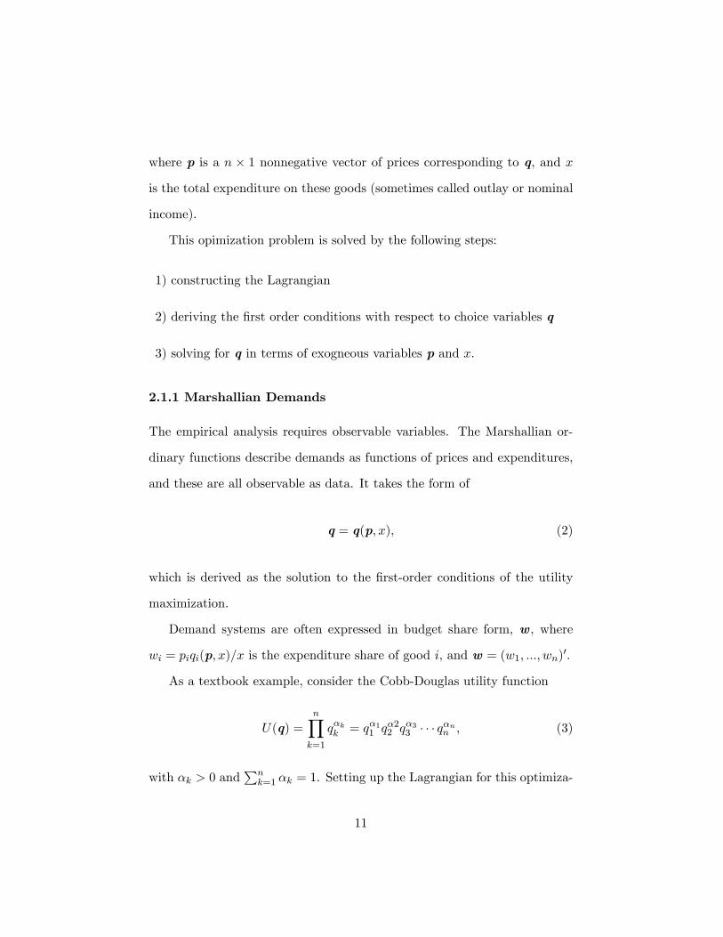
where p is a n � 1 nonnegative vector of prices corresponding to q, and x
is the total expenditure on these goods (sometimes called outlay or nominal
income).
This opimization problem is solved by the following steps:
1) constructing the Lagrangian
2) deriving the �rst order conditions with respect to choice variables q
3) solving for q in terms of exogneous variables p and x.
2.1.1 Marshallian Demands
The empirical analysis requires observable variables. The Marshallian or-
dinary functions describe demands as functions of prices and expenditures,
and these are all observable as data. It takes the form of
q = q(p; x), (2)
which is derived as the solution to the �rst-order conditions of the utility
maximization.
Demand systems are often expressed in budget share form, w, where
wi = piqi(p; x)=x is the expenditure share of good i, and w = (w1; :::; wn)0.
As a textbook example, consider the Cobb-Douglas utility function
U(q) =
nYk=1
q�kk = q�11 q�22 q�33 � � � q�nn , (3)
with �k > 0 andPnk=1 �k = 1. Setting up the Lagrangian for this optimiza-
11
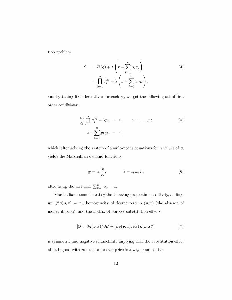
tion problem
L = U(q) + �
x�
nXk=1
pkqk
!(4)
=nYk=1
q�kk + �
x�
nXk=1
pkqk
!;
and by taking �rst derivatives for each qi, we get the following set of �rst
order conditions:
�iqi
nQk=1
q�kk � �pi = 0, i = 1; :::; n; (5)
x�nXk=1
pkqk = 0,
which, after solving the system of simultaneous equations for n values of q,
yields the Marshallian demand functions
qi = �ix
pi, i = 1; :::; n, (6)
after using the fact thatPnk=1 �k = 1.
Marshallian demands satisfy the following properties: positivity, adding-
up (p0q(p; x) = x), homogeneity of degree zero in (p; x) (the absence of
money illusion), and the matrix of Slutsky substitution e¤ects
�S = @q(p; x)=@p0 + (@q(p; x)=@x) q(p; x)0
�(7)
is symmetric and negative semide�nite implying that the substitution e¤ect
of each good with respect to its own price is always nonpositive.
12
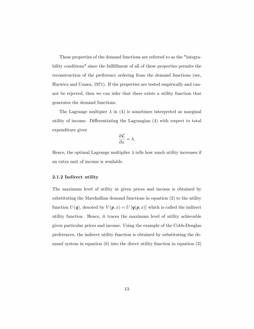
These properties of the demand functions are referred to as the "integra-
bility conditions" since the full�llment of all of these properties permits the
reconstruction of the preference ordering from the demand functions (see,
Hurwicz and Uzawa, 1971). If the properties are tested empirically and can-
not be rejected, then we can infer that there exists a utility function that
generates the demand functions.
The Lagrange multipier � in (4) is sometimes interpreted as marginal
utility of income. Di¤erentiating the Lagrangian (4) with respect to total
expenditure gives@L@x
= �:
Hence, the optimal Lagrange multiplier � tells how much utility increases if
an extra unit of income is available.
2.1.2 Indirect utility
The maximum level of utility at given prices and income is obtained by
substituting the Marshallian demand functions in equation (2) to the utility
function U(q), denoted by V (p; x) = U [q(p; x)] which is called the indirect
utility function. Hence, it traces the maximum level of utility achievable
given particular prices and income. Using the example of the Cobb-Douglas
preferences, the indirect utility function is obtained by substituting the de-
mand system in equation (6) into the direct utility function in equation (3)
13
to get
V (p; x) =nYk=1
q�kk
=nYk=1
�kPnj=1 �j
x
pk
!�k
= xnYk=1
��kpk
��k, (8)
again usingPnk=1 �k = 1.
The direct utility function and the indirect utility function are equivalent
representations of the underlying preference pre-ordering. In fact, there is
a duality relationship between the direct utility function and the indirect
utility function, in the sense that maximization of U(q) with respect to q
given (p; x) �xed, and the minimization of V (p; x) with respect to (p; x),
given q �xed, leads to the same demand functions.
Being able to represent preferences by the indirect utility function has
its advantages. As a statistical convenience, the indirect utility function has
prices as exogenous in explaining consumer behavior.10 Moreover, using V ,
we can easily derive the demand system by straightforward di¤erentiation,
without having to solve a system of simultaneous equations, as would be the
case with the direct utility function�s �rst-order conditions. In particular,
Roy�s identity,
q(p; x) = �@V (p; x)=@p@V (p; x)=@x
, (9)
allows us to derive the demand system, provided that there is an interior
10 Inverse demand systems assume that the prices are endogenous and depend on demandgoods as exogenous variables.
14
solution and that p > 0 and x > 0. Alternatively, the logarithmic form of
Roy�s identity,
w(p; x) =�@ lnV (p; x)=@ lnp@ lnV (p; x)=@ lnx
, (10)
or Diewert�s (1974, p.126) modi�ed version of Roy�s identity,
wi(�) =�irV (�)� 0rV (�) (11)
or
wi(p; x) = �@V (p; x) =@ ln pi@V (p; x) =@ lnx
;
can be used to derive the budget share equations, where � = [�1; :::; �n]0 is a
vector of expenditure normalized prices, with ith element being �i = pi=x,
and rV (�) = @V (�)=@�. The indirect utility function is continuous in
(p; x) and has the following properties: homogeneity of degree zero in (p; x),
decreasing in p and increasing in x, strictly quasiconvex in p, and it satis�es
Roy�s identity in equation (9). The equation (11) tells that the budget shares
(or quantities demanded) will never become negative if V is merely non-
decreasing in � while they could be still positive, for example, if @V=@�i < 0
for all i = 1; :::; n. Therefore, positivity of the quantity variables does not
imply the monotonicity of indirect utility function.
In the terminology of Caves and Christensen (1980), indirect utility func-
tion is regular at a given (p; x), at which it satis�es quasiconcavity and
monotonicity, provided that other axioms of consumer demand functions
are satis�ed. Similarly, the "regular region" is the set of prices and income
at which an indirect utility function satis�es the regularity conditions.
15
2.1.3 Hicksian demands
The utility maximization problem is dual to the problem of minimizing the
cost or expenditure necessary to attain a �xed level of utility u, given market
prices p:11
E(u;p) = minqp0q subject to U(q) � u. (12)
Given Cobb-Douglas preferences, the Lagrangian for this minimization
problem is
L =nXk=1
pkqk + �
u�
nYk=1
q�kk
!,
with the following set of �rst order conditions:
pi � ��iqi
nYk=1
q�kk = 0, i = 1; :::; n;
u�nYk=1
q�kk = 0,
which, solving the system of n+1 simultaneous equations for q and �, yields
the expenditure minimizing demands
qci (u;p) = u�ipi
nYk=1
�pk�k
��k, i = 1; :::; n. (13)
The expenditure minimizing demands are also known as Hicksian or com-
pensated demands. They tell us how q is a¤ected by prices with u held
11We use the term "expenditure" function for consumer demand context and "cost"function for producer input demand context and use notations E and C respectively tomaintain the consistent use of terminology.
16
constant. Finally, substituting the Hicksian demands into the expenditure
function in (12) yields
E(u;p) =
nXk=1
pkqck
=
nXj=1
pj
"u�jpj
nYk=1
�pk�k
��k#
= u
nYk=1
�pk�k
��k; (14)
usingPnk=1 �k = 1.
In general, assuming that the expenditure function is di¤erentiable with
respect to p, Shephard�s (1953) lemma,
qc(u;p) =@E(u;p)
@p, (15)
can be applied to obtain the expenditure minimizing demands qc(u;p). Al-
ternatively, the logarithmic form of Shephard�s lemma obtains the budget
share equations,
wc(u;p) =@ lnE(u;p)
@ lnp. (16)
For example, applying Shephard�s lemma (15) to the expenditure function
in equation (14), it is easy to see that Hicksian demands in equation (13)
are obtained.
Hicksian demands are positive valued and have the following properties:
homogeneity of degree zero in p, and the Slutsky matrix, [@qc(u;p)=@p0], is
symmetric and negative semide�nite.
17
Finally, the expenditure function, E(u;p) = p0qc(u;p), has the following
properties: continuous in (u;p), homogeneous of degree one in p, increasing
in p and u, concave in p, and satis�es Shephard�s lemma in equation (15).
2.1.4 Elasticity Relations
A demand system provides a complete characterization of consumer pref-
erences and can be used to estimate the income elasticities, the own-and
cross-price elasticities, as well as the elasticities of substitution. These elas-
ticities are particularly useful in judging the validity of the parameter es-
timates which are sometimes di¢ cult to interpret due to the complexity of
the demand system speci�cations, unlike regressions of linear speci�cations
where each coe¢ cient (parameter) often has a particular interpretation.
The elasticity measures can be calculated from the Marshallian demand
functions, q = q(p; x). In particular, the income elasticity of demand for
i = 1; ::; n, is calculated as
�ix(p; x) =@qi(p; x)
@x
x
qi(p; x)=@ ln qi(p; x)
@ lnx. (17)
If �ix(p; x) > 0, the ith good is classi�ed as normal at (p; x), and if �ix(p; x) <
0, it is classi�ed as inferior. Another dividing line in classifying goods ac-
cording to their income elasticities is the number one. If �ix(p; x) > 1; the
ith good is classi�ed as a necessity. For example, with Cobb-Douglas prefer-
ences represented by direct utility function of (3) and with constant elasticity
of substitution (CES) preferences also used in chapter 3, �ix(p; x) = 1 (for
all i) since Marshallian demands in this case are linear in income. One of
18
the properties of income elasticity is derived by di¤erentiating the budget
constraint with respect to x :
nXk=1
wk�kx = 1.
For i; j = 1; :::; n, the uncompensated (Cournot) price elasticities, �ij(p; x),
can be calculated as
�ij(p; x) =@qi(p; x)
@pj
pjqi(p; x)
=@ ln qi(p; x)
@ ln pj. (18)
If �ij(p; x) > 0, the goods are gross substitutes meaning that when qj be-
comes more expensive, the consumer increases consumption of good qi and
decreases consumption of good qj .12 If �ij(p; x) < 0, they are gross comple-
ments meaning that when qj becomes more expensive, the consumer reduces
the consumption of qj and also of qi. If �ij(p; x) = 0, they are independent.
Di¤erentiating the budget constraint with respect to pi yields one of the
identity properties relating the uncompensated price elasticities and budget
shares of all goods,
wi +nXk=1
wk�ki = 0:
With Cobb-Douglas preferences represented by the direct utility function of
(3), using the Marshallian demands in equation (6), the own-price elasticities
are �ii = ��i (x=piqi), and the cross-price elasticities are �ij = 0, since the
demands for the ith good depends only on the ith price.
12Two goods are said to be net substitutes if the notion is applied to compensated(Hicksian) demands.
19
The de�nitions given above are in gross terms, because they ignore the
income e¤ect, that is, the change in demand of good qi due to the change
in purchasing power resulting from the change in the price of good qj . The
Slutsky equation, however, decomposes the total e¤ect of a price change
on demand into a substitution e¤ect and an income e¤ect. In particular,
di¤erentiating the second identity in
qi(p; x) = qi (p; E(u;p)) = qci (u;p);
with respect to pj using the chain rule, noting that x = E, and rearranging,
we acquire the Slutsky equation,
@qi(p; x)
@pj=@qci (u;p)
@pj� qj(p; x)
@qi(p; x)
@x; (19)
for all (p; x), u = V (p; x), and i; j = 1; :::; n.13 The derivative @qi(p; x)=@pj
is the total e¤ect of a price change on demand, while the �rst term, @qci (u;p)=@pj
is the substitution e¤ect of a compensated price change on demand, and
�qj(p; x)@qi(p; x)=@x in the second term is the income e¤ect, resulting
from a change in price. Hicks (1936) suggested using the sign of the cross-
substitution e¤ect to classify goods as substitutes, whenever @qci (u;p)=@pj
is positive. In fact, according to Hicks (1936), @qci (u;p)=@pj > 0 indi-
cates substitutability, @qci (u;p)=@pj < 0 indicates complementarity, and
@qci (u;p)=@pj = 0 indicates independence.
One important property of the Slutsky equation is that the cross-substitution
e¤ects are symmetric expressed as @qci (u;p)=@pj = @qcj(u;p)=@pi. This sym-
13This derivation of Slutsky decomposition was due to Cook (1972).
20
metry restriction may also be written in elasticity terms.14 It is easy to verify
that the Slutsky substitution matrix can be rewritten in terms of elasticities
as
wi�ij + wiwj�ix = wj�ji + wiwj�jx;
and therefore the symmetry restriction may be written as
�ix +�ijwj
= �jx +�jiwi. (20)
The notion of elasticity of substitution was developed mainly in the pro-
ducer context to study the evolution of relative factor shares in a growing
economy. A logarithmic derivative of a quantity ratio with respect to a mar-
ginal rate of technical substitution is an intuitive measure of curvature of an
isoquant and provides information about the comparative statics of factor
shares. Out of two generalizations for more than two inputs suggested by
Allen and Hicks (1934), only one is currently used. That notion became
known as the Allen-Uzawa elasticity of substitution after Uzawa (1962) pro-
vided a more general formulation in the dual in terms of derivatives of the
cost function. He expressed the elasticity of substitution between goods i
and j as
�AUij =EEijEiEj
,
14Other useful results include:
@wi@ ln pj
= wi�ij + wi�ij ;
@wi@ lnx
= wi�ix � wi;
where �ij = 1 when i = j, or �ij = 0 otherwise.
21
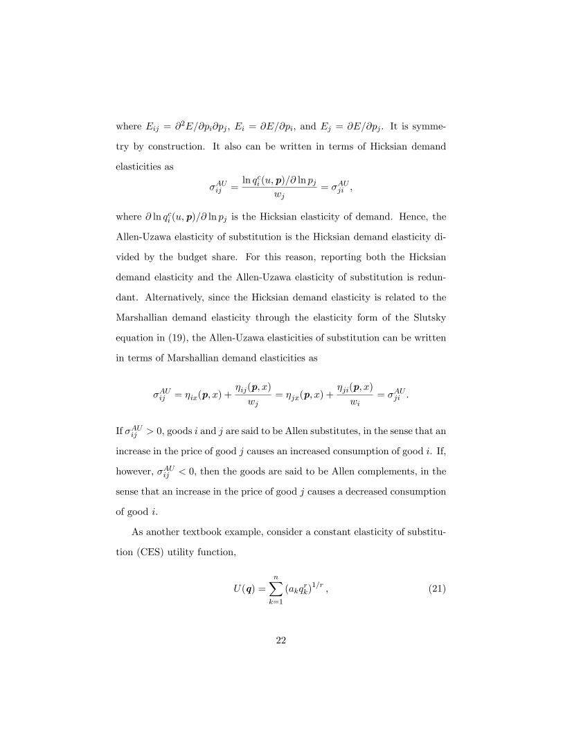
where Eij = @2E=@pi@pj , Ei = @E=@pi, and Ej = @E=@pj . It is symme-
try by construction. It also can be written in terms of Hicksian demand
elasticities as
�AUij =ln qci (u;p)=@ ln pj
wj= �AUji ;
where @ ln qci (u;p)=@ ln pj is the Hicksian elasticity of demand. Hence, the
Allen-Uzawa elasticity of substitution is the Hicksian demand elasticity di-
vided by the budget share. For this reason, reporting both the Hicksian
demand elasticity and the Allen-Uzawa elasticity of substitution is redun-
dant. Alternatively, since the Hicksian demand elasticity is related to the
Marshallian demand elasticity through the elasticity form of the Slutsky
equation in (19), the Allen-Uzawa elasticities of substitution can be written
in terms of Marshallian demand elasticities as
�AUij = �ix(p; x) +�ij(p; x)
wj= �jx(p; x) +
�ji(p; x)
wi= �AUji .
If �AUij > 0, goods i and j are said to be Allen substitutes, in the sense that an
increase in the price of good j causes an increased consumption of good i. If,
however, �AUij < 0, then the goods are said to be Allen complements, in the
sense that an increase in the price of good j causes a decreased consumption
of good i.
As another textbook example, consider a constant elasticity of substitu-
tion (CES) utility function,
U(q) =nXk=1
(akqrk)1=r , (21)
22
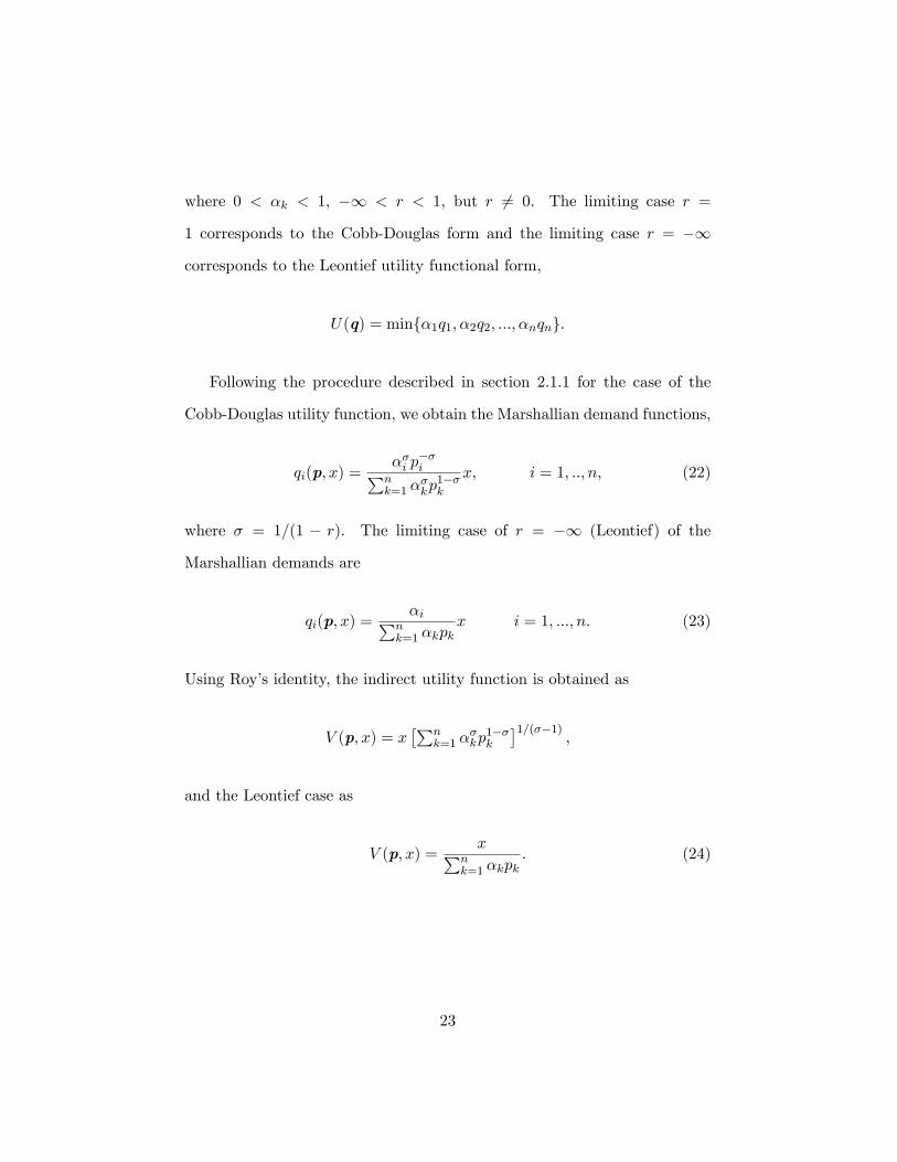
where 0 < �k < 1, �1 < r < 1, but r 6= 0. The limiting case r =
1 corresponds to the Cobb-Douglas form and the limiting case r = �1
corresponds to the Leontief utility functional form,
U(q) = minf�1q1; �2q2; :::; �nqng.
Following the procedure described in section 2.1.1 for the case of the
Cobb-Douglas utility function, we obtain the Marshallian demand functions,
qi(p; x) =��i p
��iPn
k=1 ��kp1��k
x, i = 1; ::; n; (22)
where � = 1=(1 � r). The limiting case of r = �1 (Leontief) of the
Marshallian demands are
qi(p; x) =�iPn
k=1 �kpkx i = 1; :::; n. (23)
Using Roy�s identity, the indirect utility function is obtained as
V (p; x) = x�Pn
k=1 ��kp1��k
�1=(��1),
and the Leontief case as
V (p; x) =xPn
k=1 �kpk. (24)
23
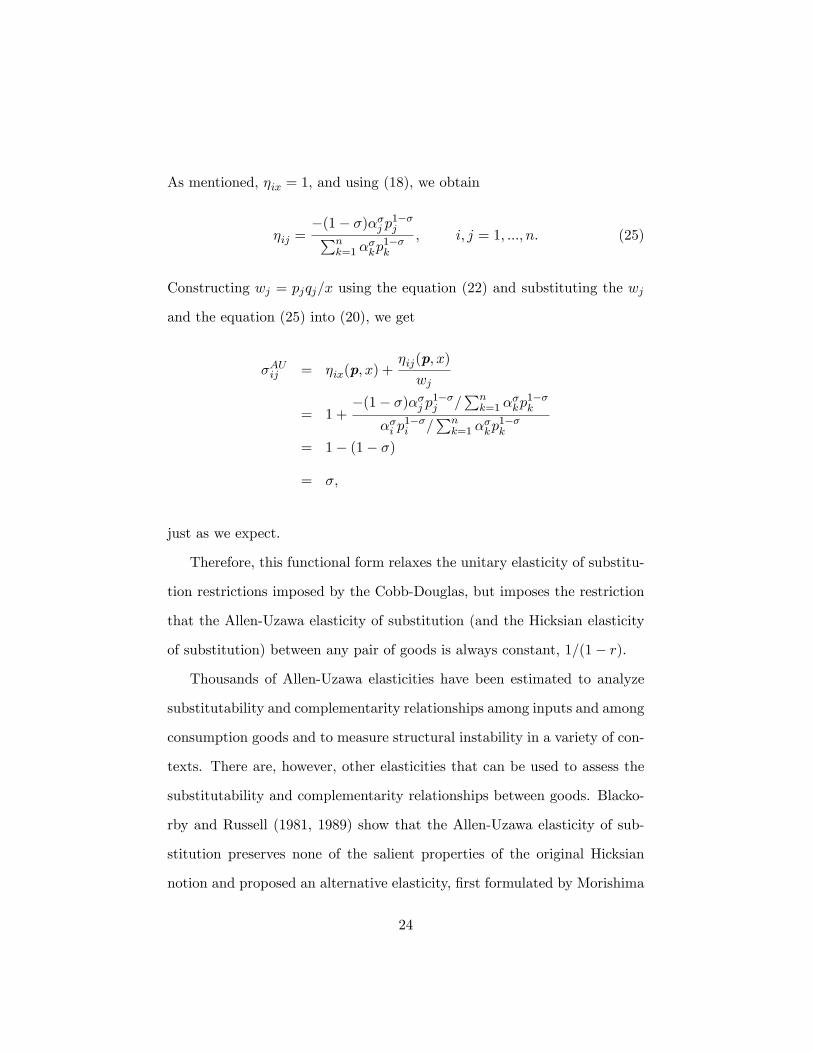
As mentioned, �ix = 1, and using (18), we obtain
�ij =�(1� �)��j p1��jPn
k=1 ��kp1��k
; i; j = 1; :::; n. (25)
Constructing wj = pjqj=x using the equation (22) and substituting the wj
and the equation (25) into (20), we get
�AUij = �ix(p; x) +�ij(p; x)
wj
= 1 +�(1� �)��j p1��j =
Pnk=1 �
�kp1��k
��i p1��i =
Pnk=1 �
�kp1��k
= 1� (1� �)
= �,
just as we expect.
Therefore, this functional form relaxes the unitary elasticity of substitu-
tion restrictions imposed by the Cobb-Douglas, but imposes the restriction
that the Allen-Uzawa elasticity of substitution (and the Hicksian elasticity
of substitution) between any pair of goods is always constant, 1=(1� r).
Thousands of Allen-Uzawa elasticities have been estimated to analyze
substitutability and complementarity relationships among inputs and among
consumption goods and to measure structural instability in a variety of con-
texts. There are, however, other elasticities that can be used to assess the
substitutability and complementarity relationships between goods. Blacko-
rby and Russell (1981, 1989) show that the Allen-Uzawa elasticity of sub-
stitution preserves none of the salient properties of the original Hicksian
notion and proposed an alternative elasticity, �rst formulated by Morishima
24
(1967). The Morishima elasticity of substitution is shown to be the natural
generalization of the original notion of Hicks when there are more than two
inputs (goods). They suggest that the Morishima elasticity of substitution is
the natural generalization of the original Hicksian concept. The Morishima
elasticity of substitution is gradually making its way into the empirical stud-
ies on substitutability and complementarity. Davis and Gauger (1996) show
how three di¤erent elasticity measures reach di¤erent conclusions on substi-
tutability/complementarity relationships in monetary assets.
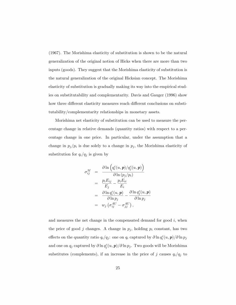
Morishima net elasticity of substitution can be used to measure the per-
centage change in relative demands (quantity ratios) with respect to a per-
centage change in one price. In particular, under the assumption that a
change in pj=pi is due solely to a change in pj , the Morishima elasticity of
substitution for qi=qj is given by
�Mij =@ ln
�qci (u;p)=q
cj(u;p)
�@ ln (pj=pi)
=piEijEj
� piEiiEi
=@ ln qci (u;p)
@ ln pj�@ ln qcj(u;p)
@ ln pj
= wj��AUij � �AUjj
�,
and measures the net change in the compensated demand for good i, when
the price of good j changes. A change in pj , holding pi constant, has two
e¤ects on the quantity ratio qi=qj : one on qi captured by @ ln qci (u;p)=@ ln pj
and one on qj captured by @ ln qcj(u;p)=@ ln pj . Two goods will be Morishima
substitutes (complements), if an increase in the price of j causes qi=qj to
25
decrease (increase). Comparing the Allen-Uzawa and Morishima elastici-
ties of substitution, we see that if two goods are Allen-Uzawa substitutes,
�AUij > 0, they must also be Morishima substitutes, �Mij > 0. However, two
goods may be Allen-Uzawa complements, �AUij < 0, but Morishima sub-
stitutes if����AUjj ��� > ����AUij ���. It suggestes that the Allen-Uzawa elasticity of
substitution matrix is symmetric, �AUij = �AUji , but the Morishima elastic-
ity of substitution matrix is not. The Morishima elasticity of substitution
matrix is symmetric only when the aggregator function is a member of the
constant elasticity of substitution family.
The Morishima elasticity of substitution is a "two-good one-price" elas-
ticity of substitution, unlike the Allen-Uzawa elasticity of substitution, which
is a "one-good one-price" elasticity of substitution. They di¤er in that the
former measures elasticities of ratios of variables rather than those of vari-
ables themselves. Another "two-good one-price" elasticity of substitution
that can be used to assess the substitutability/complementarity relationship
between goods is the Mundlak elasticity of substitution (Mundlak, 1968),
�MUij =
@ ln (qi(p; x)=qj(p; x))
@ ln (pi=pj)
= �ij(p; x)� �jj(p; x)
= �Mij + wj��jx(p; x) + �ix(p; x)
�.
The Mundlak elasticity of substitution, like the Marshallian demand elas-
ticity, is a measure of gross substitution (with income held constant). Two
goods will be Mundlak substitutes (complements) if an increase in the price
of j causes qi=qj to decrease (increase).
26
Another kind of elasticity of substitution which is "two-good two-price"
elasticity of substitution is Shadow elasticity of substitution (McFadden,
1963). It is de�ned as the negative of the elasticity of the demand ratio
qi(p; x)=qj(p; x) with respect to a change in the price ratio pi=pj holding
utility level, all other prices, and total expenditure constant. It takes the
form,
�Sij = �@ ln (qi (p; x) =qj (p; x))@ ln (pi=pj)
�����u;E and pk;k 6=i;j, constant
=�Eii=E2i + 2 (Eij=EiEj)� Ejj=E2j
1=piEi + 1=pjEj; (26)
=wj�
Mij + wj�
Mji
wi + wj; (27)
for i; j = 1; :::; n: The Shadow elasticity of substitution measures the curva-
ture of a level surface of the expenditure function in a particular direction
� such that �iqi + �jqj = 0, and �k = 0 for k 6= i; j in two-dimensional
subspace of the price space spanned by the ith and jth basis vectors. It
follows that �Sij = 0 for all i; j = 1; :::; n; i 6= j directly from the concavity of
the expenditure function.
The further generalization of Shadow elasticity of substitution was for-
mulated by Frenger (1978, 1985a, 1985b), who de�ned the directional shadow
elasticity of substitution. This elasticity measures the curvature of the level
surface of the expenditure function at a point p for an arbitrary price change
� which leaves total expenditure and utility constant. One de�nition based
27
on this idea is given by
�Dij (�) = �Pni=1
Pnj=1Eij�i�jPn
i=1 qi�i (�i=pi); � 2 T (p) ; � 6= 0.
For each p this elasticity is a function de�ned on the tangent plane T (p) =n�j�0q = 0
oto the level surface of the expenditure function at p. The
domain of �Dij (�) is all of T (p) except for the point � = 0, and �Dij (�) is
a homogeneous function of degree zero in �. It is shown that �Dij (�) = 0
for every � 2 T (p), and that it reduces to �Sij when �iqi + �jqj = 0 and
�k 6= 0; k 6= i; j:
2.1.5 Curvature
Often time, we would like to check if the functional form of demand models
has a correct curvature property. The condition can be translated to the
de�niteness of the Slutsky substitution matrix or the Allen-Uzawa elasticity
of substitution matrix. Since the de�nition of the de�niteness of matrix
is not applicable in practice, the popular method to check the de�niteness
is to apply the Cholesky factorization and check the signs of the resulting
Cholesky values. For example, the Hermitian (symmetric with real entries)
matrix is negative semi-de�nite if the all Cholesky values are nonpositive.
Lau (1978b, p. 427) shows that every positive semi-de�nite matrix A
has the following representation (Cholesky factorization):
A = LDL0; (28)
28
where L is a unit lower triangular matrix with all diagonal entries unity and
D is a diagonal matrix with all the main diagonal entries nonnegative. The
diagonal entries in D are called Cholesky values.
Because rank of the Slutsky matrix and the Allen-Uzawa elasticity ma-
trix is n�1 due to the homogeneity condition, the condition is applied to the
(n� 1) by (n� 1) matrix resulting from removing jth row and jth column
from the original substitution matrix.15 Noting that the matrix D can be
always written as D1=2D1=2 because of the non-negative diagonal entries,
the equation (28) can be written as,
A = LDL0 = LD1=2D1=2L0=�LD1=2
��LD1=2
�0= BB0; (29)
where B is some lower triangular matrix (See also Theorem 9 in Diewert
and Wales, 1987).
Alternatively, the eigenvalues of Slutsky matrix can be used to check its
negative semi-de�niteness: the eigenvalues of negative semi-de�nite matrix
are all nonpositive. The representation in (29) is more convenient than (28)
if one wants to impose the semi-de�niteness on the matrix A. It simply
requires the speci�cation of lower triangular matrix B, which is easier than
specifying L and D in (28).
In the case of three goods, given the Allen-Uzawa substitution matrix
�AU , after deleting any one row and the corresponding column, say third,
15See Moschini�s (1997) Lemma that S is negative semi-de�nite matrix if and only if eSwhose jth row and jth column are removed from S is negative semi-de�nite matrix.
29
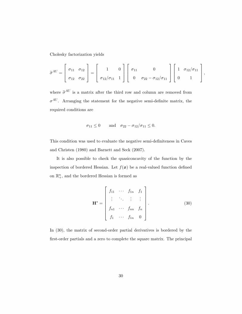
Cholesky factorization yields
e�AU =264 �11 �12
�12 �22
375 =264 1 0
�12=�11 1
375264 �11 0
0 �22 � �12=�11
375264 1 �12=�11
0 1
375 ,where e�AU is a matrix after the third row and column are removed from
�AU . Arranging the statement for the negative semi-de�nite matrix, the
required conditions are
�11 � 0 and �22 � �12=�11 � 0.
This condition was used to evaluate the negative semi-de�niteness in Caves
and Christen (1980) and Barnett and Seck (2007).
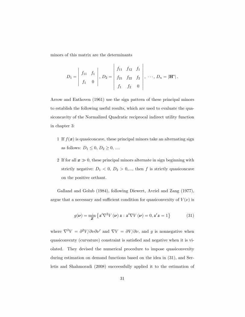
It is also possible to check the quasiconcavity of the function by the
inspection of bordered Hessian. Let f(x) be a real-valued function de�ned
on Rn+, and the bordered Hessian is formed as
H� =
266666664
f11 � � � f1n f1...
. . ....
...
fn1 � � � fnn fn
f1 � � � f1n 0
377777775. (30)
In (30), the matrix of second-order partial derivatives is bordered by the
�rst-order partials and a zero to complete the square matrix. The principal
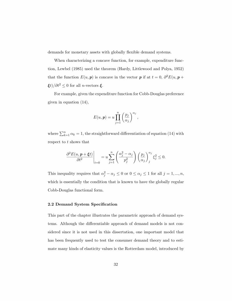
30
minors of this matrix are the determinants
D1 =
�������f11 f1
f1 0
������� , D2 =����������f11 f12 f1
f21 f22 f2
f1 f2 0
����������, � � � , Dn = jH�j .
Arrow and Enthoven (1961) use the sign pattern of these principal minors
to establish the following useful results, which are used to evaluate the qua-
siconcavity of the Normalized Quadratic reciprocal indirect utility function
in chapter 3:
1 If f(x) is quasiconcave, these principal minors take an alternating sign
as follows: D1 � 0, D2 � 0, ....
2 If for all x� 0, these principal minors alternate in sign beginning with
strictly negative: D1 < 0, D2 > 0,..., then f is strictly quasiconcave
on the positive orthant.
Galland and Golub (1984), following Diewert, Avriel and Zang (1977),
argue that a necessary and su¢ cient condition for quasiconvexity of V (�) is
g(�) = minZ
�z0r2V (�) z : z0rV (�) = 0;z0z = 1
(31)
where r2V = @2V=@�@� 0 and rV = @V=@�, and g is nonnegative when
quasiconvexty (curvature) constraint is satis�ed and negative when it is vi-
olated. They devised the numerical procedure to impose quasiconvexity
during estimation on demand functions based on the idea in (31), and Ser-
letis and Shahmoradi (2008) succeessfully applied it to the estimation of
31
demands for monetary assets with globally �exible demand systems.
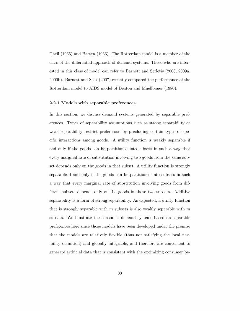
When characterizing a concave function, for example, expenditure func-
tion, Lewbel (1985) used the theorem (Hardy, Littlewood and Polya, 1952)
that the function E(u;p) is concave in the vector p if at t = 0, @2E(u;p+
�t)=@t2 � 0 for all n-vectors �.
For example, given the expenditure function for Cobb-Douglas preference
given in equation (14),
E(u;p) = unYj=1
�pj�j
��j,
wherePnk=1 �k = 1, the straightforward di¤erentiation of equation (14) with
respect to t shows that
@2E(u;p+ �t)
@t2
�����t=0
= unXj=1
�2j � �jp2j
!�pj�j
��jj
�2j � 0.
This inequality requires that �2j � �j � 0 or 0 � �j � 1 for all j = 1; :::; n,
which is essentially the condition that is known to have the globally regular
Cobb-Douglas functional form.
2.2 Demand System Speci�cation
This part of the chapter illustrates the parametric approach of demand sys-
tems. Although the di¤erentiable approach of demand models is not con-
sidered since it is not used in this dissertation, one important model that
has been frequently used to test the consumer demand theory and to esti-
mate many kinds of elasticity values is the Rotterdam model, introduced by
32
Theil (1965) and Barten (1966). The Rotterdam model is a member of the
class of the di¤erential approach of demand systems. Those who are inter-
ested in this class of model can refer to Barnett and Serletis (2008, 2009a,
2000b). Barnett and Seck (2007) recently compared the performance of the
Rotterdam model to AIDS model of Deaton and Muellbauer (1980).
2.2.1 Models with separable preferences
In this section, we discuss demand systems generated by separable pref-
erences. Types of separability assumptions such as strong separability or
weak separability restrict preferences by precluding certain types of spe-
ci�c interactions among goods. A utility function is weakly separable if
and only if the goods can be partitioned into subsets in such a way that
every marginal rate of substitution involving two goods from the same sub-
set depends only on the goods in that subset. A utility function is strongly
separable if and only if the goods can be partitioned into subsets in such
a way that every marginal rate of substitution involving goods from dif-
ferent subsets depends only on the goods in those two subsets. Additive
separability is a form of strong separability. As expected, a utility function
that is strongly separable with m subsets is also weakly separable with m
subsets. We illustrate the consumer demand systems based on separable
preferences here since those models have been developed under the premise
that the models are relatively �exible (thus not satisfying the local �ex-
ibility de�nition) and globally integrable, and therefore are convenient to
generate arti�cial data that is consistent with the optimizing consumer be-
33
haviors.16 Since this dissertation is not concerned with any of the issues
on separability, we give only a brief note on the literature before illustrat-
ing the several models with separable preference. Leontief (1947a, 1947b)
investigated the underlying mathematical structure of separability in the
producer context and Sono (1945) in the consumer context. Debreu (1960)
provided an important characterization of additivity. The notions of weak
and strong separability were developed in Strotz (1957, 1959) and Gorman
(1959). Goldman and Uzawa (1964) developed a characterization of separa-
bility in terms of the partial derivatives of the demand functions. Gorman
(1968) provides a de�nitive discussion of separability concepts. One may
enjoy reading the subsequent exchange between Vind (1971a, 1971b) and
Gorman (1971a, 1971b). Blackorby, Primont and Russel (1978) provide a
thorough discussion and rigorous analysis of separability. There is a large
amount of literature on the empirical examination of separable preference
structures. Most of the nonparametric tests that have been developed are
based on Varian (1982, 1983, 1985). Works on tests for weak separability in
the producer model include Berndt and Christensen (1973, 1974), Berndt
and Wood (1975), Denny and Fuss (1977), Woodland (1987), Blackorby,
Schworm and Fisher (1986), Diewert and Wales (1995). In the consumer
context, works on tests of separability include Jorgenson and Lau (1975).
Large numbers of studies are interested in the separability of the monetary
aggregates from other aggregate variables.17 Monte Carlo studies that assess
16Blackorby, Primont and Russell (1977, 1978) showed that if we start with any �exiblefunctional form, then under the hypothesis of weak separability, the resulting functionwould be necessarily in�exible.17See Fisher and Fleissig (1997), Fleissig and Swo¤ord (1996), Fleissig and Whitney
(2003), Jones and Stracca (2006), Swo¤ord and Whitney (1987, 1988, 1994).
34
the performance of the various available tests of separability include Barnett
and Choi (1983), Elger, Jones and Binner (2006). O (2008) investigates the
performances of several non-parametric tests including the newly developed
de Peretti�s (2005) test.
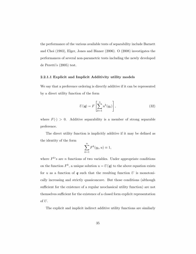
2.2.1.1 Explicit and Implicit Additivity utility models
We say that a preference ordering is directly additive if it can be represented
by a direct utility function of the form
U(q) = F
"nXk=1
uk(qk)
#, (32)
where F (�) > 0. Additive separability is a member of strong separable
preference.
The direct utility function is implicitly additive if it may be de�ned as
the identity of the formnXk=1
F k(qk; u) � 1;
where F k�s are n functions of two variables. Under appropriate conditions
on the function F k, a unique solution u = U(q) to the above equation exists
for u as a function of q such that the resulting function U is monotoni-
cally increasing and strictly quasiconcave. But those conditions (although
su¢ cient for the existence of a regular neoclassical utility function) are not
themselves su¢ cient for the existence of a closed form explicit representation
of U .
The explicit and implicit indirect additive utility functions are similarly
35
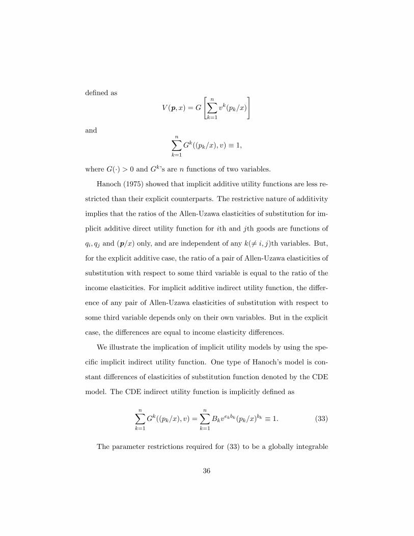
de�ned as
V (p; x) = G
"nXk=1
vk(pk=x)
#
andnXk=1
Gk((pk=x); v) � 1;
where G(�) > 0 and Gk�s are n functions of two variables.
Hanoch (1975) showed that implicit additive utility functions are less re-
stricted than their explicit counterparts. The restrictive nature of additivity
implies that the ratios of the Allen-Uzawa elasticities of substitution for im-
plicit additive direct utility function for ith and jth goods are functions of
qi; qj and (p=x) only, and are independent of any k(6= i; j)th variables. But,
for the explicit additive case, the ratio of a pair of Allen-Uzawa elasticities of
substitution with respect to some third variable is equal to the ratio of the
income elasticities. For implicit additive indirect utility function, the di¤er-
ence of any pair of Allen-Uzawa elasticities of substitution with respect to
some third variable depends only on their own variables. But in the explicit
case, the di¤erences are equal to income elasticity di¤erences.
We illustrate the implication of implicit utility models by using the spe-
ci�c implicit indirect utility function. One type of Hanoch�s model is con-
stant di¤erences of elasticities of substitution function denoted by the CDE
model. The CDE indirect utility function is implicitly de�ned as
nXk=1
Gk((pk=x); v) =
nXk=1
Bkvekbk(pk=x)
bk � 1: (33)
The parameter restrictions required for (33) to be a globally integrable
36
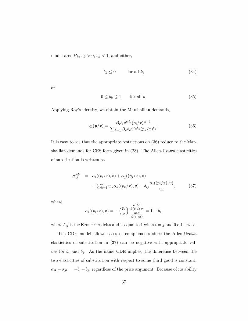
model are: Bk, ek > 0, bk < 1, and either,
bk � 0 for all k; (34)
or
0 � bk � 1 for all k. (35)
Applying Roy�s identity, we obtain the Marshallian demands,
qi(p=x) =Bibiv
eibi(pi=x)bi�1Pn
k=1Bkbkvekbk(pk=x)bk
: (36)
It is easy to see that the appropriate restrictions on (36) reduce to the Mar-
shallian demands for CES form given in (23). The Allen-Uzawa elasticities
of substitution is written as
�AUij = �i((pi=x); v) + �j((pj=x); v)
�Pnk=1wk�k((pk=x); v)� �ij
�i((pi=x); v)
wi; (37)
where
�i((pi=x); v) = ��pix
� @2Gi
@(pi=x)2
@Gi
@(pi=x)
= 1� bi,
where �ij is the Kronecker delta and is equal to 1 when i = j and 0 otherwise.
The CDE model allows cases of complements since the Allen-Uzawa
elasticities of substitution in (37) can be negative with appropriate val-
ues for bi and bj . As the name CDE implies, the di¤erence between the
two elasticities of substitution with respect to some third good is constant,
�ik��jk = �bi+ bj , regardless of the price argument. Because of its ability
37
to be globally regular and to represent complementary relationship of goods,
the linear homogeneous CDE when ei = e for all i, is used to generate the
arti�cial demand data that is consistent with rational consumer behavior in
Jensen (1997) and Barnett and Usui (2007) as well as in chapter 3.
Despite the fact that greater theoretical �exibility per free parameter is
sometimes possible by specifying and restricting implicit utility functions
rather than explicit utility functions, the attempt to use the model in prac-
tice faces an immediate obstacle. After observing that the construction of
a unique and estimable structural model from an underlying implicit util-
ity function is troublesome since it does not have an explicit closed form
solution for the implied reduced form of the demand system, one notices
that the conventional maximum likelihood estimation with additive error
structure cannot be used. Barnett, Kopecky and Sato (1981) managed to
estimate the direct implicit addilog model (DIA). See Barnett (1981, chapter
9) for detailed discussion of their highly promising, but not yet successfully
implemented approach.
2.2.1.2 WS-Branch Utility Demand System
The Barnett�s (1977) nonhomothetic WS-branch utility tree is the general-
ization to blockwise strong separability of the S-branch utility tree (Brown
and Heien, 1972). In view of (32), the block utility function uk�s are of the
generalized CES form and the aggregator utility function F is CES. The
WS-branch model is the only blockwise weakly separable utility function
and can be shown to be a �exible form when there are no more than two
goods in each block and a total of no more than two blocks. It is homo-
38
thetic in supernumerary quantities, but not homothetic in the elementary
quantities. Hence, a homothetic utility function can be converted into a
nonhomothetic utility function by translating the quantities into supernu-
merary quantities. In this model, the individual aggregator (or category)
functions within the tree are in the form of the generalized quadratic mean
of order �, as in the macro-utility function de�ned over those aggregates.
Therefore, this functional form can represent a wide range of preferences
when the number of goods in the system is no more than four. Barnett and
Choi (1989), Barnett and Seck (2007) and O (2008) used the WS-branch
tree to generate the arti�cial data for their Monte Carlo studies.
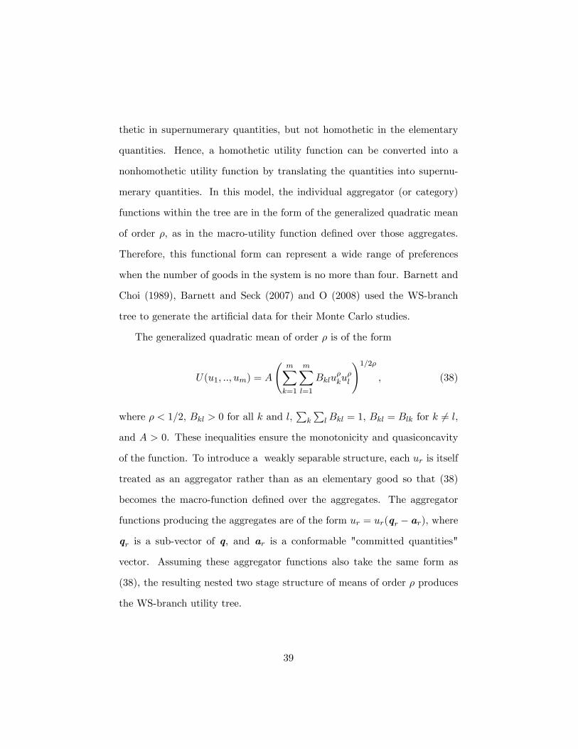
The generalized quadratic mean of order � is of the form
U(u1; ::; um) = A
mXk=1
mXl=1
Bklu�ku�l
!1=2�, (38)
where � < 1=2, Bkl > 0 for all k and l,Pk
PlBkl = 1, Bkl = Blk for k 6= l,
and A > 0. These inequalities ensure the monotonicity and quasiconcavity
of the function. To introduce a weakly separable structure, each ur is itself
treated as an aggregator rather than as an elementary good so that (38)
becomes the macro-function de�ned over the aggregates. The aggregator
functions producing the aggregates are of the form ur = ur(qr � ar), where
qr is a sub-vector of q, and ar is a conformable "committed quantities"
vector. Assuming these aggregator functions also take the same form as
(38), the resulting nested two stage structure of means of order � produces
the WS-branch utility tree.
39
2.2.2 Locally Flexible Functional Forms
A locally �exible functional form is a second-order approximation to an
arbitrary function. In the demand system literature there are two di¤er-
ent de�nitions of second-order approximations, one by Diewert (1971) and
another by Lau (1974). Barnett (1983b) has identi�ed the relationship of
each of those de�nitions to existing de�nitions in the mathematics of lo-
cal approximation orders and has shown that a second-order Taylor series
approximation is su¢ cient but not necessary for both Diewert�s and Lau�s
de�nitions of second-order approximation.
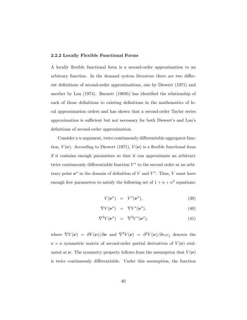
Consider a n-argument, twice continuously di¤erentiable aggregator func-
tion, V (�). According to Diewert (1971), V (�) is a �exible functional form
if it contains enough parameters so that it can approximate an arbitrary
twice continuously di¤erentiable function V � to the second order at an arbi-
trary point �� in the domain of de�nition of V and V �. Thus, V must have
enough free parameters to satisfy the following set of 1 + n+ n2 equations:
V (��) = V �(��), (39)
rV (��) = rV �(��), (40)
r2V (��) = r2V �(��), (41)
where rV (�) = @V (�)=@� and r2V (�) = @2V (�)=@�i�j denotes the
n � n symmetric matrix of second-order partial derivatives of V (�) eval-
uated at �. The symmetry property follows from the assumption that V (�)
is twice continuously di¤erentiable. Under this assumption, the function
40
does not have to satisfy all n2 equations in (41) independently since the
symmetry of second derivatives (sometimes known as Young�s theorem)
implies that @2V (��)=@�i@�j = @2V (��)=@�j@�i and @2V (�)=@�i@�j =
@2V (�)=@�j@�i for all i and j. Thus the matrices of second order par-
tial derivatives r2V (��) = r2V �(��) are both symmetric matrices. Hence,
there are only n(n + 1)=2 independent equations to be satis�ed in the re-
strictions (41), so that a general locally �exible functional form must have
at least 1 + n+ n(n+ 1)=2 free parameters.
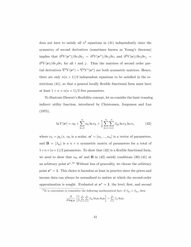
To illustrate Diewert�s �exibility concept, let us consider the basic translog
indirect utility function, introduced by Christensen, Jorgenson and Lau
(1975),
lnV (�) = �0 +nXk=1
�k ln �k +1
2
nXk=1
nXl=1
�kl ln �k ln �l; (42)
where �k = pk=x, �0 is a scalar, �0 = [�1; :::; �n] is a vector of parameters,
and B = [�kl] is a n � n symmetric matrix of parameters for a total of
1+n+(n+1)=2 parameters. To show that (42) is a �exible functional form,
we need to show that �0, �0 and B in (42) satisfy conditions (39)-(41) at
an arbitrary point ��.18 Without loss of generality, we choose the arbitrary
point �� = 1. This choice is harmless at least in practice since the prices and
income data can always be normalized to unities at which the second-order
approximation is sought. Evaluated at �� = 1, the level, �rst, and second
18 It is convenient to remember the following mathematical fact: if �kl = �lk, then
@
@ log pi
�1
2
nPk=1
nPl=1
�kl ln pk ln pl
�=
nPl=1
�il ln pl:
41
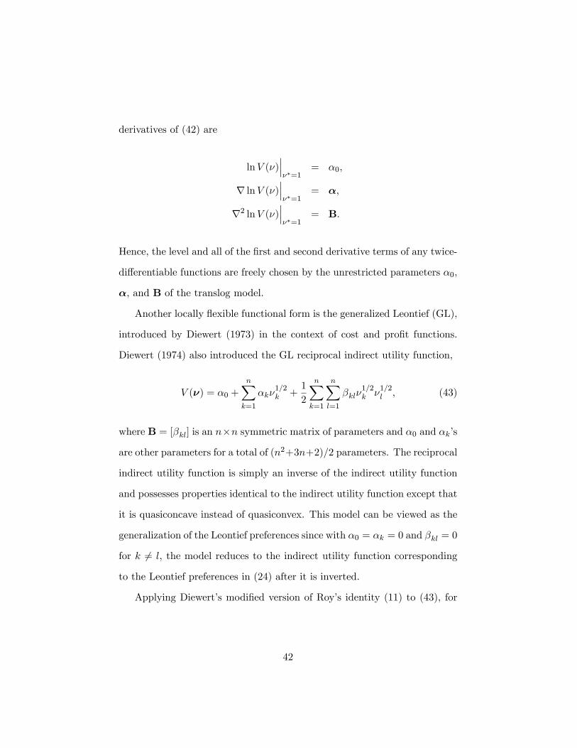
derivatives of (42) are
lnV (�)�����=1
= �0;
r lnV (�)�����=1
= �;
r2 lnV (�)�����=1
= B.
Hence, the level and all of the �rst and second derivative terms of any twice-
di¤erentiable functions are freely chosen by the unrestricted parameters �0,
�, and B of the translog model.
Another locally �exible functional form is the generalized Leontief (GL),
introduced by Diewert (1973) in the context of cost and pro�t functions.
Diewert (1974) also introduced the GL reciprocal indirect utility function,
V (�) = �0 +
nXk=1
�k�1=2k +
1
2
nXk=1
nXl=1
�kl�1=2k �
1=2l , (43)
where B = [�kl] is an n�n symmetric matrix of parameters and �0 and �k�s
are other parameters for a total of (n2+3n+2)=2 parameters. The reciprocal
indirect utility function is simply an inverse of the indirect utility function
and possesses properties identical to the indirect utility function except that
it is quasiconcave instead of quasiconvex. This model can be viewed as the
generalization of the Leontief preferences since with �0 = �k = 0 and �kl = 0
for k 6= l, the model reduces to the indirect utility function corresponding
to the Leontief preferences in (24) after it is inverted.
Applying Diewert�s modi�ed version of Roy�s identity (11) to (43), for
42
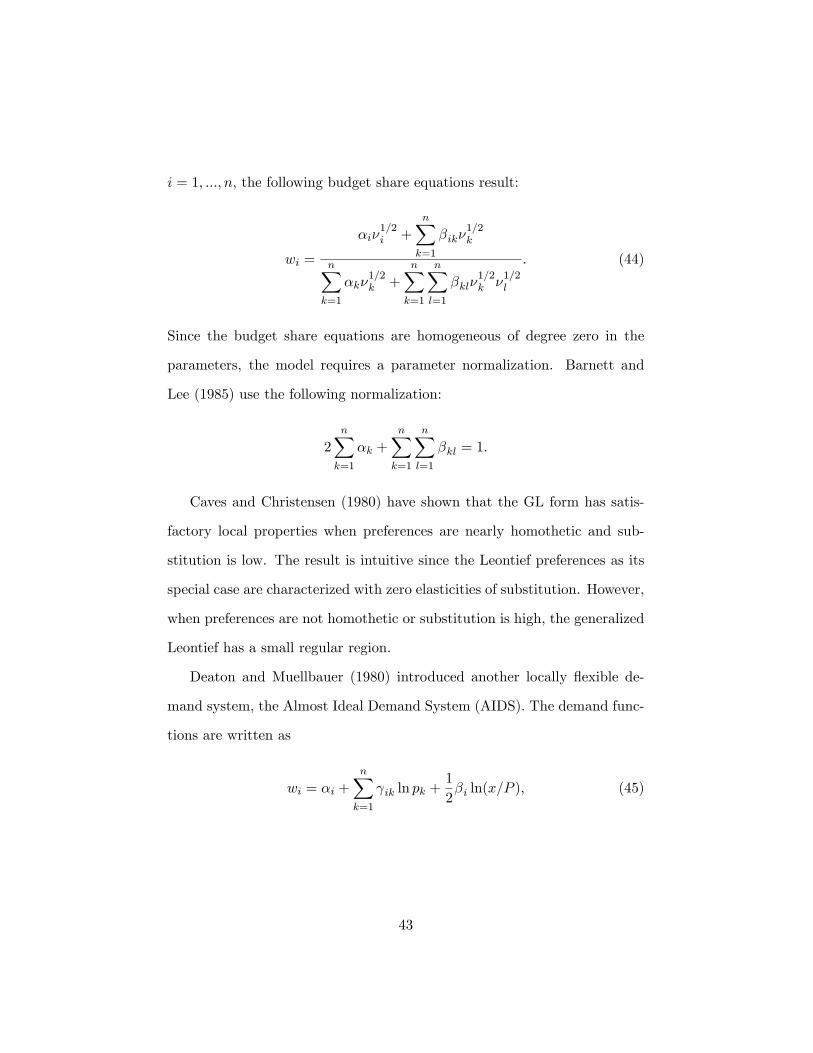
i = 1; :::; n, the following budget share equations result:
wi =
�i�1=2i +
nXk=1
�ik�1=2k
nXk=1
�k�1=2k +
nXk=1
nXl=1
�kl�1=2k �
1=2l
. (44)
Since the budget share equations are homogeneous of degree zero in the
parameters, the model requires a parameter normalization. Barnett and
Lee (1985) use the following normalization:
2nXk=1
�k +nXk=1
nXl=1
�kl = 1.
Caves and Christensen (1980) have shown that the GL form has satis-
factory local properties when preferences are nearly homothetic and sub-
stitution is low. The result is intuitive since the Leontief preferences as its
special case are characterized with zero elasticities of substitution. However,
when preferences are not homothetic or substitution is high, the generalized
Leontief has a small regular region.
Deaton and Muellbauer (1980) introduced another locally �exible de-
mand system, the Almost Ideal Demand System (AIDS). The demand func-
tions are written as
wi = �i +
nXk=1
ik ln pk +1
2�i ln(x=P ), (45)
43
for i = 1; :::; n; where the price de�ator of the logarithm of income is
lnP = �0 +nXk=1
�k ln pk +1
2
nXk=1
nXl=1
kl ln pk ln pl.
For more details regarding the AIDS, see Deaton and Muellbauer (1980),
Barnett and Serletis (2008), and Barnett and Seck (2008).
2.2.3 Engel Curves and the Rank of Demand Systems
Applied demand analysis uses two types of data: time series and cross sec-
tional data. Time series data o¤er substantial variation in relative prices
and less variation in income, whereas cross-sectional data o¤er limited vari-
ation in relative prices and substantial variation in income levels. In time
series data, prices and income vary simultaneously, whereas, in household
budget data prices are almost constant. Household budget data give rise to
the Engel curves (income expansion paths), which are functions describing
how a consumer�s purchase of goods vary as the consumer�s income varies.
Engel curves are Marshallian demand functions, with prices of all goods
held constant. Like Marshallian demand functions, Engel curves may also
depend on demographic or other non-income consumer characteristics (such
as, for example, age and household composition), which we have chosen to
ignore in this section.
Engel curves can be used to calculate the income elasticity of a good and
hence whether a good is an inferior, normal, or luxury good, depending on
whether income elasticity is less than zero, between zero and one, or greater
than one, respectively. They are also used for equivalence scale calculations
44
(welfare comparisons across households) and for determining properties of
demand systems, such as aggregability and rank. For many commodities,
standard empirical demand systems do not provide an accurate picture of
observed behavior across income groups.
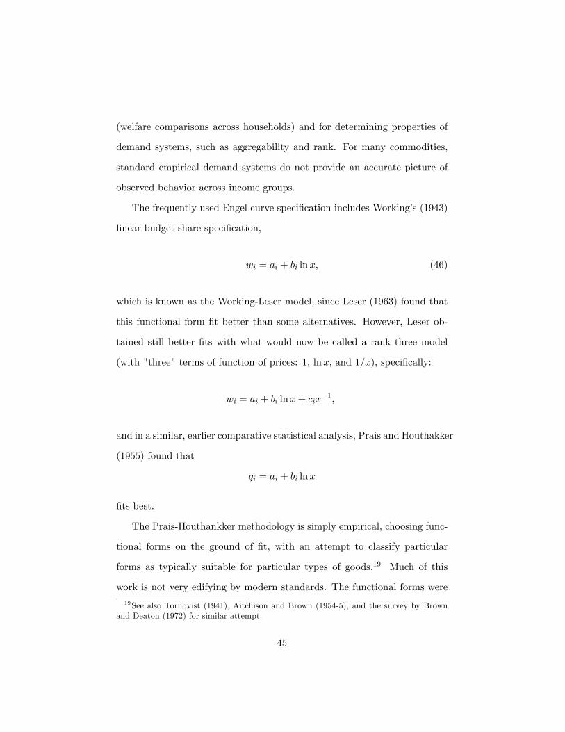
The frequently used Engel curve speci�cation includes Working�s (1943)
linear budget share speci�cation,
wi = ai + bi lnx, (46)
which is known as the Working-Leser model, since Leser (1963) found that
this functional form �t better than some alternatives. However, Leser ob-
tained still better �ts with what would now be called a rank three model
(with "three" terms of function of prices: 1, lnx, and 1=x), speci�cally:
wi = ai + bi lnx+ cix�1,
and in a similar, earlier comparative statistical analysis, Prais and Houthakker
(1955) found that
qi = ai + bi lnx
�ts best.
The Prais-Houthankker methodology is simply empirical, choosing func-
tional forms on the ground of �t, with an attempt to classify particular
forms as typically suitable for particular types of goods.19 Much of this
work is not very edifying by modern standards. The functional forms were
19See also Tornqvist (1941), Aitchison and Brown (1954-5), and the survey by Brownand Deaton (1972) for similar attempt.
45
rarely chosen with any theoretical model in mind. Indeed, all but one of
Prais and Houthakker�s Engel curves are incapable of satisfying the adding-
up requirement, while on the econometric side, satisfactory methods for
comparing di¤erent (non-nested) functional forms were not well-developed.
Even the apparently straightforward comparison between a double-log and
a linear speci�cation led to considerable di¢ culties; see the simple statis-
tic proposed by Sargan (1964) and the theoretically more satisfactory (but
extremely complicated) solution in Aneuryn-Evans and Deaton (1980).
However, these empirical results give a motivation to construct a plau-
sible functional form of demand functions that also satis�es the axioms of
consumer demand behavior. Using (16) in which the budget shares are the
logarithmic derivatives of the expenditure function, the Engel curve of the
form in equation (46) corresponds to the di¤erential equations of the form
@ lnE(u;p)
@ ln pi= �i(p) + �i(p) lnE(u;p), (47)
which gives a solution of the general form
lnE(u;p) = u ln b(p) + (1� u) ln a(p), (48)
where �i(p) = (ai ln b�bi ln a)=(ln b�ln a) and �i(p) = bi=(ln b�ln a) for ai =
@ ln a=@ ln pi and bi = @ ln b=@ ln pi. The form in (48) gives the expenditure
function as a utility-weighted geometric mean of the linear homogeneous
functions a(p) and b(p) representing the expenditure functions of the very
poor (u = 0) and the very rich (u = 1), respectively. Such preferences have
46
been called the PIGLOG (price independent generalized logarithmic) class
by Muellbauer (1975), (1976a), (1976b). A full system of demand equations
within the class of Working-Leser form can be generated by a suitable choice
of the functions a(p) and b(p). Functional forms of the log translog (See
Pollak and Wales, 1992) and the AIDS model in (45) are members of the
PIGLOG class with particular choices of the two homogeneous functions.
For example, if
ln a(p) = a0 +nXk=1
�k ln pk +1
2
nXk=1
nXl=1
kl ln pk ln pl,
and
ln b(p) = ln a(p) + �0
nYk=1
p�kk ,
we obtain the AIDS model of Deaton and Muellbauer (1980) in (45).
The log translog (log TL) indirect utility function is given by
V (p; x) = �nXk=1
�k ln (pk=x)�1
2
nXk=1
nXl=1
�kl ln (pk=x) ln (pl=x) , (49)
for all k; l = 1; :::; n, where
�kl = �lk,nXk=1
nXl=1
�kl = 0,nXk=1
�k = 1,
47
The corresponding share equations are given by
wi(p; x) =
�i +
nXk=1
�ik ln pk � lnxnXk=1
�ik
1 +
nXk=1
nXl=1
�kl ln pk ln pl
(50)
for i = 1; :::; n. Since the log TL share equations in (50) are linear in the
logarithm of expenditure, the log TL belongs to the PIGLOG class.
2.2.4 Exact Aggregation
We begin our discussion of the rank of demand systems with the de�nition
of exactly aggregable demand systems. A demand system is "exactly ag-
gregable" if demands can be summed across consumers to yield closed form
expressions for aggregate demand. Exactly aggregable demand systems are
demand systems that are linear in functions of income, as follows:
wi(p; x) =RXr=1
cir(p)'r(x); (51)
where cir(p)�s are the coe¢ cients on 'r(x), which is a scalar valued function
independent of p, and R is a positive integer. Gorman (1981), extending
earlier results by Muellbauer (1975, 1976a), proved in the context of exactly
aggregable demand systems that integrability forces the matrix of Engel
curve coe¢ cients to have rank three or less. The rank of a matrix is de�ned
as the maximum number of linearly independent columns. Other related
exact aggregation theorems can be found in Banks, Blundell and Lewbel
(1997).
48
2.2.5 The Rank of Demand Systems
Lewbel (1991) extended Gorman�s rank idea to all demand systems, not
just exactly aggregable demand systems by de�ning the rank of a demand
system to be the dimension of the space spanned by its Engel curves, holding
demographic or other non-income consumer characteristics �xed. He showed
that demands that are not exactly aggregable can have rank higher than
three and still be consistent with utility maximization.
Formally, the rank of any given demand system is the smallest value of
R such that each wi can be written as
wi(p; x) =RXr=1
�ir(p)fr(p; x); (52)
for some R � n, where for each r = 1; :::; R, �ir is a function of prices and
fr is a scalar valued function of prices and income. That is, the rank of the
system is the number of linearly independent vectors of price functions. All
demand systems have rank R � n, where n is the number of goods. Clearly,
demands that are not exactly aggregable can have rank greater than three
(i.e., R > 3). Equation (52) is a generalization of the concept of rank. That
generalization, de�ned by Gorman (1981), only applies to exactly aggregable
demands. Notice that 'r in equation (51) is not a function of p.
Hence, any demand system has rank R, if there exist R goods such that
the Engel curve of any good equals a weighted average of the Engel curves
of those R goods. The rank of an integrable demand system determines
the number of price functions on which the indirect utility function and the
cost or expenditure function depend. Lewbel calls the form in (52) Gorman
49
Engel curves.
We can see the implication that higher order terms in theoretically plau-
sible polynomial demand systems must satisfy severe restrictions by consid-
ering the implications of the Slutsky symmetry conditions for third degree
polynomial demand systems:
wi = ci0 (p) + ci1(p) lnx+ ci2(p) ln2 x+ ci3 (p) ln
3 x.
It is straightforward to calculate the Slutsky terms corresponding to this
demand system as@wi@ ln pj
+ wj@wi@ lnx
,
in share term for i; j = 1; :::; n.20 These Slutsky terms are polynomials
of degree �ve in lnx and, because symmetry holds as an identity in the
price-income space, symmetry must hold for the coe¢ cients of like powers
of lnx. To illustrate our point, it su¢ ces to calculate only that portion of
the Slutsky term of degree four in lnx. Note that the �fth polynomial term
in lnx is given by 3ci3cj3, so symmetry of this term imposes no restrictions
on the coe¢ cients of the demand system. The term of degree of four is given
by
2ci2cj3 + 3ci3cj2;
or equivalently,
(2ci2cj3 + 2ci3cj2) + ci3cj2.
20 @qi@pj
+ qj@qi@x
= (x=pipj)�
@wi@ ln pj
+ wj@wi@ ln x
+ wiwj � �ijwi�where �ij = 1 when i = j
and 0 otherwise.
50
Because the term in brackets is symmetric, symmetry of this equation im-
pliesci3ci2
=cj3cj2.
Hence, the ratio of the coe¢ cient of the cubic terms to the coe¢ cients of
the quadratic terms will be constant across equations since this condition is
applied to any pair of equations. Hausman, Newly and Powell (1995) test
whether or not a rank four speci�cation gives any additional information by
estimating,
wi = �0 + �1 lnx+ �2 ln2 x+ �3 ln
3 x+ "i.
If the demand system is rank three, the ratio �2=�3 (Gorman statistics)
should be constant for any equations. They in fact �nd this ratio is almost
perfectly constant despite considerable variation in the estimates of �2�s and
the �3�s.
2.2.5.1 Demand Systems Proportional to Expenditure
Homothetic demand systems, with Engel curves being rays from the origin,
have rank one. Rank one demand systems, such as the Cobb-Douglas, CES,
and homothetic translog, exhibit expenditure proportionality (so that the
budget share of every good is independent of total expenditure). This con-
tradicts Engel�s law, according to which the budget share of food is smaller
for rich than for poor households.
Rank one demand systems can be written as
qi(p; x) = bi(p)x
51
and are homothetic. For example, the demand system of the Cobb-Douglas
utility function (3) is given by (6), that of the CES utility function (21) is
qi(p; x) =p1=( �1)iPn
k=1 p =( �1)k
x,
and that of the homothetic translog can be reduced from log TL in equation
(50) after imposing the additional restrictionPnk=1 �ik = 0 for all i.
Clearly, expenditure proportionality implies marginal budget shares that
are constant and in fact equal to the average budget shares. Because of
this, the assumption of expenditure proportionality has little relevance in
empirical demand analysis.
2.2.5.2 Demand Systems Linear in Expenditure
A demand system that is linear in expenditure is of the form
qi(p; x) = ci(p) + bi(p)x.
If ci(p) = 0 (for all i) then demands are homothetic. Gorman (1961) showed
that any demand system is consistent with utility maximization and linear
in expenditure must be of the form
qi(p; x) = fi(p)�gi(p)
g(p)f(p) +
gi(p)
g(p)x
= fi(p) +gi(p)
g(p)[x� f(p)] , (53)
52
where g(p) and f(p) are functions homogeneous of degree one, and gi(p)
and fi(p) denote the partial derivative of g(p) and f(p) with respect to the
ith price. Such demand systems are generated by an indirect utility function
of the "Gorman polar form,"
V (p; x) =x� f(p)g(p)
. (54)
To see this, apply Roy�s identity (9) to (54) to get (53).
An example of a demand system linear in expenditure is the "linear
expenditure system,"
qi(p; x) = bi �aipi
nXk=1
pkbk +aipix,
generated by the (Stone-Geary) utility function,
U(q) =nXk=1
ak ln(qk � bk), ai > 0, qi � bi > 0,nXk=1
ak = 1
which is homothetic relative to the point b = [b1;:::; bn] as origin, or equiv-
alently by an indirect utility function of the Gorman polar form, (54) with
f(p) =Pnk=1 pkbk and g(p) =
Qnk=1 p
akk , with
Pnk=1 ak = 1, so that fi(p) =
bi and gi(p)=g(p) = ai=pi.
Demand systems linear in expenditure are rank two and have linear En-
gel curves, but not necessarily through the origin. Linearity in expenditure
implies marginal budget shares that are independent of the level of expen-
diture, suggesting that poor and rich households spend the same fraction of
an extra dollar on each good. This hypothesis, as well as the hypothesis of
53
expenditure proportionality, are too restrictive for the analysis of household
budget data.
2.2.5.3 Demand Systems Linear in the Logarithm of Expenditure
Muellbauer (1975) has studied "two-term" demand systems of the general
form
qi(p; x) = ci(p)x+ bi(p)f(x), (55)
for any function f(x). Homothetic demand is obtained, if f(x) = 0. He
shows that if f(x) 6= 0, then f(x) must be either equal to xk with k 6= 1
(the price independent generalized linearity (PIGL) class) or equal to x lnx
(the price independent generalized logarithmic (PIGLOG) class).
Hence, the PIGLOG class of demand systems is linear in the logarithm
of total expenditure and has the form
qi(p; x) = ci(p)x+ bi(p)x lnx,
with expenditure entering linearly and as a logarithmic function of x. Muell-
bauer (1975b) has shown that theoretically plausible demand systems of the
PIGLOG form must be written as
qi(p; x) =gi(p)
g(p)x� Gi(p)
G(p)[lnx� ln g(p)]x, (56)
where G(p) is homogeneous of degree zero, G(p) = G(�p), and g(�p) is
homogeneous of degree one, g(�p) = �g(p). The indirect utility function
54
associated with (56) is
V (p; x) = G(p) [lnx� ln g(p)] . (57)
To see this, apply Roy�s identity (9) to (57) to get (56).
Examples of PIGLOG demand systems are the log-translog (log TL), a
special case of the basic translog, and the AIDS model. It is to be noted,
however, that PIGLOG speci�cations have a rank two, and thus have limited
�exibility in modeling the curvature of Engel curves.
2.2.5.4 Demand Systems Quadratic in Expenditure
Lewbel (1987a) has studied "three-term" demand systems of the following
form:
qi(p; x) = ci(p) + bi(p)x+ ai(p)f(x). (58)
Equation (58) is a special case of Gorman�s (1981) equation (51), with r
ranging from 1 to 3 and '1(x) = 1, '2(x) = x, and '3(x) = f(x). Gor-
man�s (1981) main result, that the matrix of Engel curve coe¢ cients can-
not have rank higher than three, is true in this case, since that matrix,
[c(p) b(p) a(p)], only has three columns. Lewbel (1987a) showed that in
equation (58), f(x) must be either 0, xk, x lnx, or lnx, and that the only
f(x) that yields full rank-three demand systems is x2. Hence, one way to
relax the assumption that demand systems are linear in expenditure is to
specify demand systems that are quadratic in expenditure, as follows:
qi(p; x) = ci(p) + bi(p)x+ ai(p)x2. (59)
55
Ryan and Wales (1999), following Howe, Pollak and Wales (1979) and
van Daal and Merkies (1989), argue that for a quadratic demand system to
be theoretically plausible, the demand functions must be of the form
qi(p; x) =1
g(p)2
�ri(p)�
gi(p)
g(p)r(p)
�[x� f(p)]2
+gi(p)
g(p)[x� f(p)] + fi(p)
+�
�r(p)
g(p)
��ri(p)�
gi(p)
g(p)r(p)
�, (60)
where there are no restrictions on the function � (�), functions f(p), g(p),
and r(p) are restricted to be homogeneous of degree one in prices, and fi(p),
gi(p), and ri(p) are the �rst partial derivatives of f(p), g(p), and r(p) with
respect to pi. The demand function (60) can be simpli�ed by assuming
� (�) = 0 and de�ning r(p) to be the product of g(p) and a function h(p),
that is homogeneous of degree zero in prices, so that the coe¢ cient of the
quadratic term in (60) becomes hi(p)=g(p). In that case (60) reduces to
qi(p; x) =hi(p)
g(p)[x� f(p)]2 + gi(p)
g(p)[x� f(p)] + fi(p), (61)
and its corresponding indirect utility function is
V (p; x) = � g(p)
x� f(p) � h(p). (62)
To see this, apply Roy�s identity (9) to (62) to get (61).
Equation (62) is the general form of the indirect utility function that
can generate quadratic Engel curves (that is, rank-three demand systems).
56
The di¤erence between the Gorman polar form indirect utility function (54)
and the more general indirect utility function (62) is that the latter adds
a term, h(p), that is homogeneous of degree zero in prices, to the Gorman
polar form indirect utility function (54).
The �rst functional form proposed along these lines is the quadratic
AIDS of Bank, Blundell and Lewbel (1997) (known as QUAIDS), which we
will use for the empirical study in chapter 4. The QUAIDS is an extension of
simple AIDS, having expenditure shares linear in log income and in another
smooth function of income. See Banks, Blundell and Lewbel (1997) for more
details.
Following Banks, Blundell and Lewbel (1997), Ryan and Wales (1999)
modi�ed the translog, GL, and NQ demand systems and introduced three
new demand systems called the translog-quadratic expenditure system, the
GL-quadratic expenditure system, and the NQ-quadratic expenditure sys-
tem.
To demonstrate, we consider the NQ expenditure function (NQEF), in-
troduced by Diewert and Wales (1988b, 1993):
E(u;p) = a0p+
�b0p+
1
2
p0Bp
�0p
�u, (63)
where the parameters of the model consist of a0 = [a1; :::; an], b0 = [b1; :::; bn],
and the elements of the n�n symmetric B = [Bkl] matrix. The nonnegative
vector of predetermined parameters �0 = [�1; :::; �n] is assumed to satisfy
�0p� = 1, �i � 0 for i = 1; :::; n, (64)
57
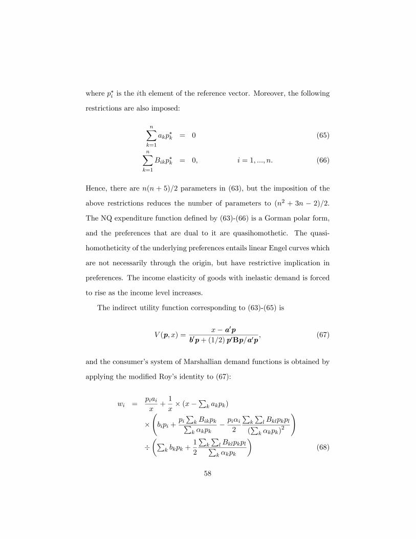
where p�i is the ith element of the reference vector. Moreover, the following
restrictions are also imposed:
nXk=1
akp�k = 0 (65)
nXk=1
Bikp�k = 0, i = 1; :::; n. (66)
Hence, there are n(n + 5)=2 parameters in (63), but the imposition of the
above restrictions reduces the number of parameters to (n2 + 3n � 2)=2.
The NQ expenditure function de�ned by (63)-(66) is a Gorman polar form,
and the preferences that are dual to it are quasihomothetic. The quasi-
homotheticity of the underlying preferences entails linear Engel curves which
are not necessarily through the origin, but have restrictive implication in
preferences. The income elasticity of goods with inelastic demand is forced
to rise as the income level increases.
The indirect utility function corresponding to (63)-(65) is
V (p; x) =x� a0p
b0p+ (1=2)p0Bp=a0p; (67)
and the consumer�s system of Marshallian demand functions is obtained by
applying the modi�ed Roy�s identity to (67):
wi =piaix+1
x� (x�
Pk akpk)
� bipi +
piPk BikpkPk �kpk
� pi�i2
Pk
PlBklpkpl
(Pk �kpk)
2
!
��P
k bkpk +1
2
Pk
PlBklpkplPk �kpk
�(68)
58
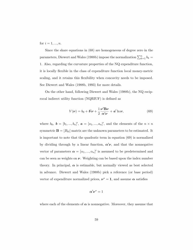
for i = 1; :::; n.
Since the share equations in (68) are homogeneous of degree zero in the
parameters, Diewert andWales (1988b) impose the normalizationPnk=1 bk =
1. Also, regarding the curvature properties of the NQ expenditure function,
it is locally �exible in the class of expenditure function local money-metric
scaling, and it retains this �exibility when concavity needs to be imposed.
See Diewert and Wales (1988b, 1993) for more details.
On the other hand, following Diewert and Wales (1988b), the NQ recip-
rocal indirect utility function (NQRIUF) is de�ned as
V (�) = b0 + b0� +
1
2
� 0B�
�0�+ a0 ln�, (69)
where b0, b = [b1; :::; bn]0, a = [a1; :::; an]
0, and the elements of the n � n
symmetricB = [Bkl]matrix are the unknown parameters to be estimated. It
is important to note that the quadratic term in equation (69) is normalized
by dividing through by a linear function, �0�, and that the nonnegative
vector of parameters � = [�1; :::; �n]0 is assumed to be predetermined and
can be seen as weights on �. Weighting can be based upon the index number
theory. In principal, � is estimable, but normally viewed as best selected
in advance. Diewert and Wales (1988b) pick a reference (or base period)
vector of expenditure normalized prices, �� = 1, and assume � satis�es
�0�� = 1
where each of the elements of � is nonnegative. Moreover, they assume that
59
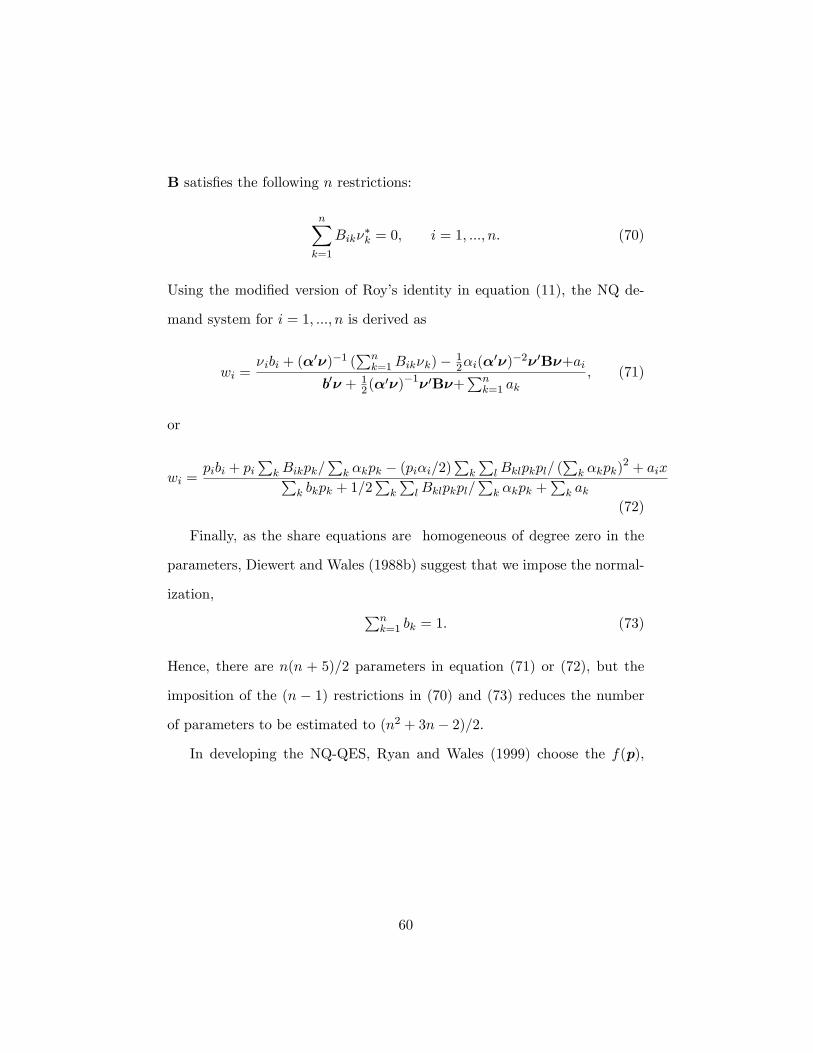
B satis�es the following n restrictions:
nXk=1
Bik��k = 0, i = 1; :::; n. (70)
Using the modi�ed version of Roy�s identity in equation (11), the NQ de-
mand system for i = 1; :::; n is derived as
wi =�ibi + (�
0�)�1 (Pnk=1Bik�k)� 1
2�i(�0�)�2� 0B�+ai
b0� + 12(�
0�)�1� 0B�+Pnk=1 ak
, (71)
or
wi =pibi + pi
Pk Bikpk=
Pk �kpk � (pi�i=2)
Pk
PlBklpkpl= (
Pk �kpk)
2 + aixPk bkpk + 1=2
Pk
PlBklpkpl=
Pk �kpk +
Pk ak
(72)
Finally, as the share equations are homogeneous of degree zero in the
parameters, Diewert and Wales (1988b) suggest that we impose the normal-
ization, Pnk=1 bk = 1: (73)
Hence, there are n(n + 5)=2 parameters in equation (71) or (72), but the
imposition of the (n � 1) restrictions in (70) and (73) reduces the number
of parameters to be estimated to (n2 + 3n� 2)=2.
In developing the NQ-QES, Ryan and Wales (1999) choose the f(p),
60
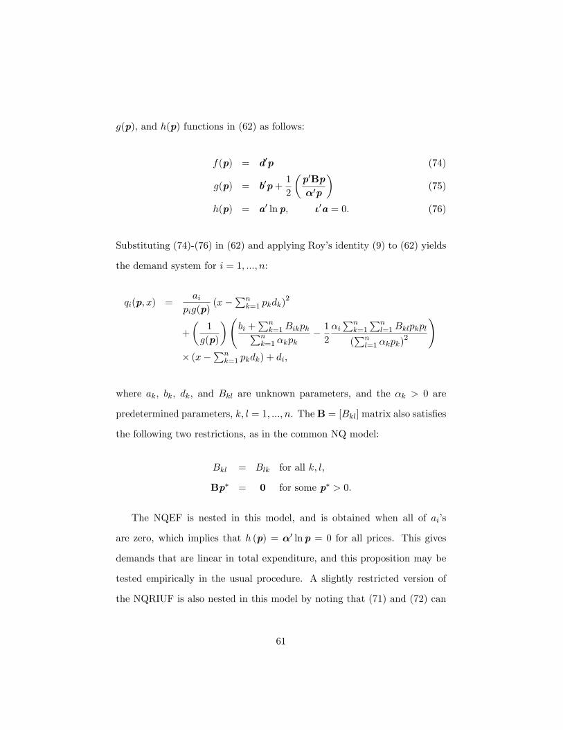
g(p), and h(p) functions in (62) as follows:
f(p) = d0p (74)
g(p) = b0p+1
2
�p0Bp
�0p
�(75)
h(p) = a0 lnp, �0a = 0. (76)
Substituting (74)-(76) in (62) and applying Roy�s identity (9) to (62) yields
the demand system for i = 1; :::; n:
qi(p; x) =ai
pig(p)(x�
Pnk=1 pkdk)
2
+
�1
g(p)
� bi +
Pnk=1BikpkPn
k=1 �kpk� 12
�iPnk=1
Pnl=1Bklpkpl
(Pnl=1 �kpk)
2
!� (x�
Pnk=1 pkdk) + di,
where ak, bk, dk, and Bkl are unknown parameters, and the �k > 0 are
predetermined parameters, k; l = 1; :::; n. TheB = [Bkl]matrix also satis�es
the following two restrictions, as in the common NQ model:
Bkl = Blk for all k; l,
Bp� = 0 for some p� > 0.
The NQEF is nested in this model, and is obtained when all of ai�s
are zero, which implies that h (p) = �0 lnp = 0 for all prices. This gives
demands that are linear in total expenditure, and this proposition may be
tested empirically in the usual procedure. A slightly restricted version of
the NQRIUF is also nested in this model by noting that (71) and (72) can
61
be rewritten using (74) to (76) as
qi (p; x) =higx2 +
gigx.
Equation (61) becomes this form when f(p) = 0.
The development of the GL-QES and TL-QES follows a similar pattern.
See Ryan and Wales (1999) for more details.
The QUAIDS, translog-quadratic expenditure system, GL-quadratic ex-
penditure system, and NQ-quadratic expenditure system are locally �exible
in the Diewert sense and also are rank-three demand systems, thereby allow-
ing more �exibility in modeling income distribution than the AIDS, translog,
GL, and NQ models.
2.2.5.5 Demand Systems Quadratic in the Logarithm of Expendi-
ture
The indirect utility function of the models that are quadratic in the loga-
rithm of expenditure is
lnV (p; x) =
"�lnx� ln a(p)
b(p)
��1+ c(p)
#�1(77)
where a; b are homogeneous of degree zero in p, and c is homogeneous of
degree one. This class of demand systems is predominantly known by the
quadratic AIDS of Bank, Blundell and Lewbel (1997) with speci�cations of
a, b, and c:
c (p) =
nXk=1
ck ln pk wherenXk=1
ck = 0
62
ln a(p) = �0 +nXk=1
�k ln pk +1
2
nXk=1
nXl=1
kl ln pk ln pl
ln b(p) =nXk=1
�k ln pk.
By Roy�s identity, the budget shares of the QUAIDS for i = 1; :::; n are given
by
wi = �i +nXk=1
ik ln pk + �i ln [x=a(p)] +cib(p)
(ln [x=a(p)])2 . (78)
The QUAIDS model has the income �exibility with rank three. The AIDS
model is nested within it as a special case when c(p) = 0.
2.2.5.6 Demand System Linear in Trigonometric Functions of Ex-
penditure
Gorman (1981) �rst conjectured that utility-derived trigonometric demand
systems would exist, without giving any examples of them. Lewbel (1988)
proved the existence of the trigonometric class of demand systems, and char-
acterized its general form alone with the underlying indirect utility function.
This class of models has the maximum rank of an exactly aggregable demand
system and o¤ers the attractive features mentioned in the previous section.
It is important to note that the Fourier �exible demand systems do not
belong to the trigonometric class in terms of forms of Engel curves.
The trigonometric demand systems are derived from the indirect utility
63
function of the form:
V (p; x) = b(p) +c(p) cos f� log [a(p)=x]g1 + sin f� log [a(p)=x]g � 6= 0,
where a(p) is homogeneous of degree one, b(p) and c(p) are homogeneous
of degree zero in p, and � is a non-zero parameter whose size should be
reasonable enough to prevent many oscillations over the range of the data.
For i = 1; :::; n the straightforward application of Roy�s identity yields
qi =
�aia� bi�c
�x+
�bi�ccos(� ln a)� ci
�csin (� ln a)
�x sin (� lnx)
��bi�csin(� ln a) +
ci�ccos (� ln a)
�x cos (� lnx) ;
and in share form,
wi =piaia� pi�cfbi + bi sin (� ln [a=x]) + ci cos (� ln [a=x])g . (79)
To derive the estimable trigonometric demand functions, Matsuda (2006)
provides the speci�cation of these price functions such that:
a(p) =
nYk=1
p�kk ; (80)
b(p) =
nXk=1
�k ln pk; (81)
c(p) =nXk=1
�k +nXk=1
nXl=1
kl ln pk ln pl, (82)
withPnk=1 �k = 1,
Pnk=1 �k = 1,
Pnk=1 kl = 0 for k = 1; :::; n to ful�l
64
adding-up and homogeneity. Slutsky symmetry is guaranteed by kl = lk
for k; l = 1; :::; n.
The share equations in (79) is rewritten using (80) to (82) as21
wi = �i ��i + fi(p) sin (� log x) + gi(p) cos(� lnx)
�c(p); (83)
where fi(p) and gi(p) are functions speci�ed as
fi(p) = 2
nXl=1
il ln pk
!sin [� ln a(p)]� �i cos [� ln a(p)] , i = 1; :::n;
gi(p) = 2
nXl=1
il ln pk
!cos [� ln a(p)] + �i sin [� ln a(p)] , i = 1; :::n.
Matsuda (2006) called the new model represented by (83) the TDS,
which stands for the trigonometric demand system. Linearity in trigonomet-
ric functions of share equations (83) allows for the aggregation of consumers
without involving linear Engel curves. Rank of the TDS is three, whereas
that of the AIDS is two. Although a �exible rank-three demand system, the
TDS has n� 1 fewer free parameters than known rank-three models such as
the QUAIDS.
2.2.5.7 Fractional demand systems
Lewbel (1987b) has studied demand systems of the "fractional" form
21The following results from the angel di¤erence fourmulas were used to derive theequation (83):
sin f� log [a(p)=x]g = sin f� log [a(p)=x]g sin f� log [a(p)=x]g�sin f� log [a(p)=x]g sin f� log [a(p)=x]g ;
cos f� log [a(p)=x]g = cos f� log [a(p)=x]g cos f� log [a(p)=x]g+cos f� log [a(p)=x]g cos f� log [a(p)=x]g :
65
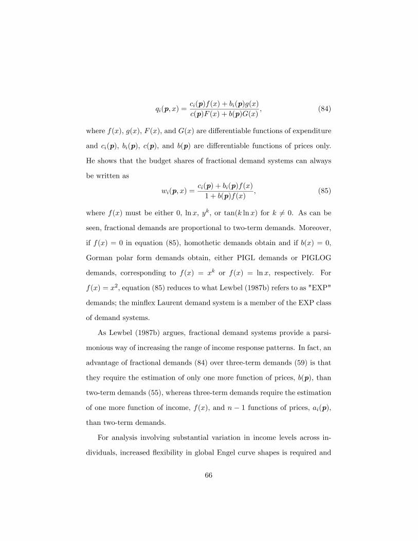
qi(p; x) =ci(p)f(x) + bi(p)g(x)
c(p)F (x) + b(p)G(x), (84)
where f(x), g(x), F (x), and G(x) are di¤erentiable functions of expenditure
and ci(p), bi(p), c(p), and b(p) are di¤erentiable functions of prices only.
He shows that the budget shares of fractional demand systems can always
be written as
wi(p; x) =ci(p) + bi(p)f(x)
1 + b(p)f(x), (85)
where f(x) must be either 0, lnx, yk, or tan(k lnx) for k 6= 0. As can be
seen, fractional demands are proportional to two-term demands. Moreover,
if f(x) = 0 in equation (85), homothetic demands obtain and if b(x) = 0,
Gorman polar form demands obtain, either PIGL demands or PIGLOG
demands, corresponding to f(x) = xk or f(x) = lnx, respectively. For
f(x) = x2; equation (85) reduces to what Lewbel (1987b) refers to as "EXP"
demands; the min�ex Laurent demand system is a member of the EXP class
of demand systems.
As Lewbel (1987b) argues, fractional demand systems provide a parsi-
monious way of increasing the range of income response patterns. In fact, an
advantage of fractional demands (84) over three-term demands (59) is that
they require the estimation of only one more function of prices, b(p), than
two-term demands (55), whereas three-term demands require the estimation
of one more function of income, f(x), and n � 1 functions of prices, ai(p),
than two-term demands.
For analysis involving substantial variation in income levels across in-
dividuals, increased �exibility in global Engel curve shapes is required and
66
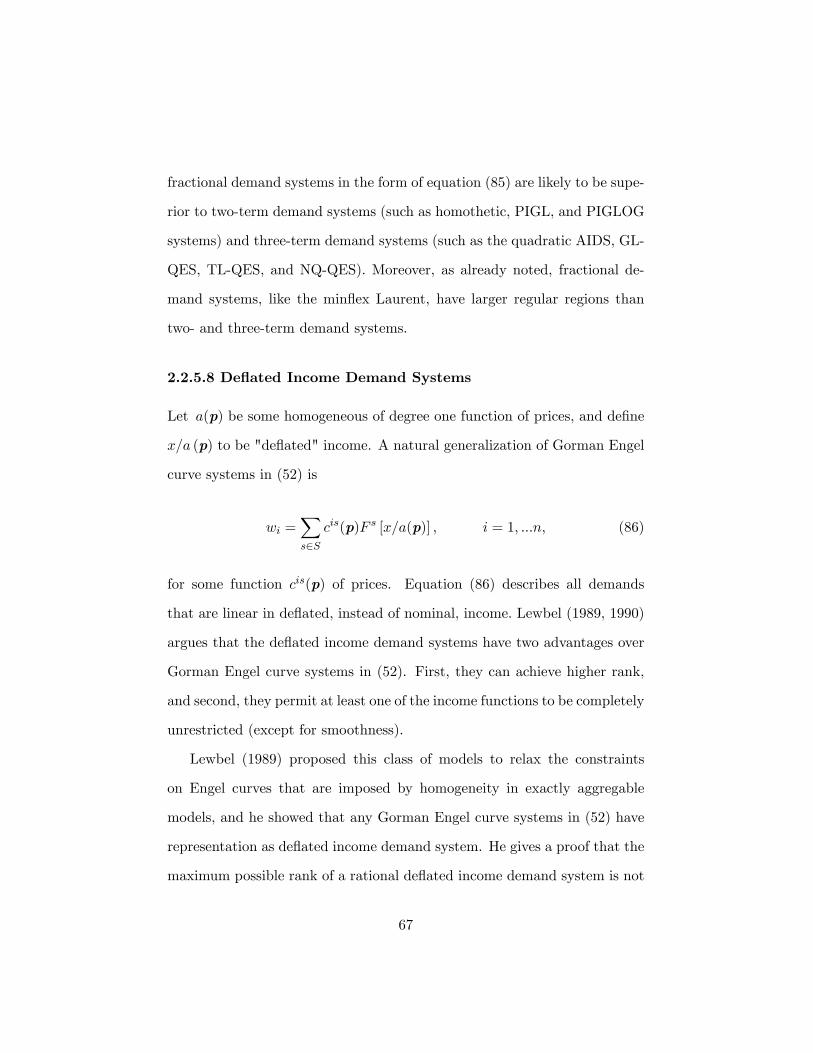
fractional demand systems in the form of equation (85) are likely to be supe-
rior to two-term demand systems (such as homothetic, PIGL, and PIGLOG
systems) and three-term demand systems (such as the quadratic AIDS, GL-
QES, TL-QES, and NQ-QES). Moreover, as already noted, fractional de-
mand systems, like the min�ex Laurent, have larger regular regions than
two- and three-term demand systems.
2.2.5.8 De�ated Income Demand Systems
Let a(p) be some homogeneous of degree one function of prices, and de�ne
x=a (p) to be "de�ated" income. A natural generalization of Gorman Engel
curve systems in (52) is
wi =Xs2S
cis(p)F s [x=a(p)] ; i = 1; :::n; (86)
for some function cis(p) of prices. Equation (86) describes all demands
that are linear in de�ated, instead of nominal, income. Lewbel (1989, 1990)
argues that the de�ated income demand systems have two advantages over
Gorman Engel curve systems in (52). First, they can achieve higher rank,
and second, they permit at least one of the income functions to be completely
unrestricted (except for smoothness).
Lewbel (1989) proposed this class of models to relax the constraints
on Engel curves that are imposed by homogeneity in exactly aggregable
models, and he showed that any Gorman Engel curve systems in (52) have
representation as de�ated income demand system. He gives a proof that the
maximum possible rank of a rational de�ated income demand system is not
67

three, but four.
Lewbel (2003) considered a nearly log polynomial rational rank four
demand system,
V (p; x) =
"�ln [x� d(p)]� a(p)
b(p)
��1+ c(p)
#�1; (87)
where a, b, c and d are functions of prices. Homogeneity requires that c and
d be homogenous of degree zero and that b and a be homogeneous of degree
one in p. Application of Roy�s identity to this indirect utility function yields
demands of the form
w =A4(p)
x+
�1� d(p)
x
� 3Xr=1
Ar(p) (ln [x� d(p)])r�1 ; (88)
where
A1(p) =@a(p)
@ lnp� @b(p)
@ lnp
a(p)
b(p)+@c(p)
@ lnp
a(p)2
b(p);
A2(p) =@b(p)
@ lnp
1
b(p)� 2@c(p)
@ lnp
a(p)
b(p);
A3(p) =@c(p)
@ lnp
1
b(p);
A4(p) =@d(p)
@ lnp.
This is a de�ated income demand system and its rank is four, provided that
no one of the functions a, b, c, or d can be written as a function of the other
three.
If d(p) = 0 for all p, then A4(p) also equals zero, and equation (88)
reduces to the quadratic logarithmic model, which is equation (78). More-
68
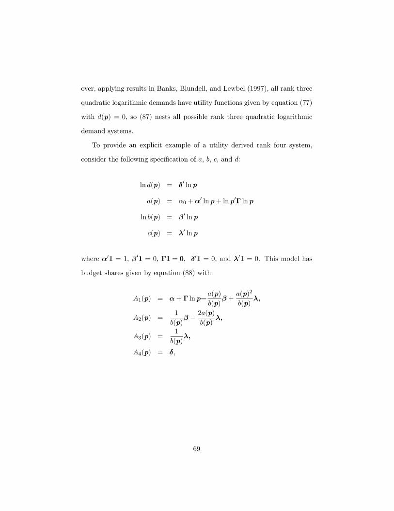
over, applying results in Banks, Blundell, and Lewbel (1997), all rank three
quadratic logarithmic demands have utility functions given by equation (77)
with d(p) = 0, so (87) nests all possible rank three quadratic logarithmic
demand systems.
To provide an explicit example of a utility derived rank four system,
consider the following speci�cation of a, b, c, and d:
ln d(p) = �0 lnp
a(p) = �0 +�0 lnp+ lnp0� lnp
ln b(p) = �0 lnp
c(p) = �0 lnp
where �01 = 1, �01 = 0, �1 = 0, �01 = 0, and �01 = 0. This model has
budget shares given by equation (88) with
A1(p) = �+ � lnp�a(p)
b(p)� +
a(p)2
b(p)�;
A2(p) =1
b(p)� � 2a(p)
b(p)�;
A3(p) =1
b(p)�;
A4(p) = �,
69
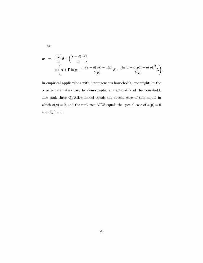
or
w =d(p)
x� +
�x� d(p)
x
�� �+ � lnp+
ln (x� d(p))� a(p)b(p)
� +(ln (x� d(p))� a(p))2
b(p)�
!:
In empirical applications with heterogeneous households, one might let the
� or � parameters vary by demographic characteristics of the household.
The rank three QUAIDS model equals the special case of this model in
which a(p) = 0, and the rank two AIDS equals the special case of a(p) = 0
and d(p) = 0.
70
Chapter 3
The Theoretical Regularity Properties of the Normalized Quadratic
Consumer Demand Model
3.1 Introduction
Uzawa (1962) proved that the constant elasticity of substitution (CES)
model cannot attain arbitrary elasticities with more than two goods. As
a result, the development of locally �exible functional forms evolved as a
new approach to modeling speci�cations of tastes and technology. Flexible
functional forms were de�ned by Diewert (1971) to be the class of functions
that have enough free parameters to provide a local second-order approxima-
tion to any twice continuously di¤erentiable function. If a �exible functional
form has no more parametric freedom than needed to satisfy that de�nition,
then the �exible functional form is called "parsimonious." Barnett (1983)
proved that a functional form satis�es Diewert�s de�nition if and only if it
can attain any arbitrary elasticities at any one predetermined point in price-
income space. Most of the available �exible functional forms are based on
quadratic forms derived from second-order series expansions. The translog
model of Christensen, Jorgenson and Lau (1971) and the AIDS model of
Deaton and Muellbauer (1980) use Taylor series expansions in logarithms;
the generalized Leontief model of Diewert (1971) uses a Taylor series ex-
pansion in square roots; and the Laurent models of Barnett (1983) use the
Laurent series expansion.
As these �exible functional form models became available, applied re-
71
searchers tended to overlook the maintained regularity conditions required
by the theory. Regularity requires satisfaction of both curvature and monotonic-
ity conditions. Simultaneous imposition of both of these conditions on a
parsimonious �exible functional form destroys the model�s local �exibility
property. For instance, Lau (1978) showed that imposition of global regu-
larity reduces the translog model to Cobb-Douglas, which is not a �exible
functional form anymore and has no estimable elasticities. When regularity
is not imposed, most of the estimated �exible functional forms in empirical
applications exhibit frequent violations of regularity conditions at many data
points.22 Since that fact became evident, information about violations of
regularity conditions in empirical applications have become hard to �nd.23
An exception to the common neglect of regularity conditions was Diewert
and Wales�(1987, 1988b) work on the Normalized Quadratic model. That
model permits imposition of curvature globally, while remaining �exible.
Since violations of curvature have more often been reported than violations
of monotonicity, the imposition of curvature alone seems to merit consider-
ation. In subsequent papers of Diewert and Wales (1993, 1995) and others,
imposition of curvature globally, without imposition of monotonicity, has be-
come a common practice with the Normalized Quadratic functional form.24
But once curvature is imposed without the imposition of monotonicity,
the earlier observation may no longer apply. When global curvature is im-
22See, e.g., Manser (1974) and Humphrey and Moroney (1975).23A noteworthy exception is Moroney and Trapani (1981), who con�rmed the earlier
�ndings of frequent violations of maintained regularity conditions.24Quah (2000) studies the monotonicity of individual and market demand with the aid
of the indirect utility function and identi�es su¢ cient conditions on an agent�s indirectutility function to guarantee that the demand function is monotonic.
72
posed, the loss of model-�t may induce spurious improvements in �t through
violations of monotonicity. This problem could be especially common with
quadratic models, which can have bliss points. It is possible that violations
of monotonicity could be induced by imposition of curvature.
With this model, it has become common not to check for monotonic-
ity after imposing global curvature. Diewert and Wales (1995) and Ryan
and Wales (1998) have expected that monotonicity will be satis�ed as a re-
sult of the non-negativity of the dependent variables. But non-negativity of
observed dependent variables does not assure non-negativity of �tted depen-
dent variables. In Kohli (1993) and Diewert and Fox (1999), the curvature
condition is treated as the sole regularity condition. But without satis-
faction of both curvature and monotonicity, the second-order condition for
optimizing behavior fails, duality theory fails, and inferences resulting from
derived estimating equations become invalid.25 Hence the common practice
of equating regularity solely with curvature is not justi�ed.
Barnett (2002) and Barnett and Pasupathy (2003) con�rmed the poten-
tial problem and found further troublesome consequences when they checked
regularity violations in their own previously published estimation of tech-
nology in the �nancial sector in Barnett, Kirova and Pasupathy (1995). Ini-
tially, they imposed curvature globally, but monotonicity only at a central
data point with the Normalized Quadratic production model. In addition
to violations of monotonicity, they encountered induced curvature reversals
of composite functions, along with nonunique isoquants and complex valued
25The damage done to the inference has been pointed out by Basmann, Molina andSlottje (1983); Basmann, Diamond, Frentrup and White (1985); Basmann, Fawson andShumway (1990); and Basmann, Hayes and Slottje (1994).
73

solutions. Even if curvature is imposed on both inner (category) production
functions and weakly separable outer functions, the composite technology
still can violate curvature if monotonicity is violated. The evidence sug-
gested the need for a thorough investigation of the global regularity property
of the Normalized Quadratic model. We undertake that task in this chapter.
A well-established approach to exploring regularity properties of a neo-
classical function is to set the parameters of the model to produce vari-
ous plausible elasticities and then plot the regular regions within which the
model satis�es monotonicity and curvature. We do so by setting the para-
meters at various levels to produce elasticities that span the plausible range
and then plot the regular region of the model when curvature is imposed
while monotonicity is not imposed. The intent is to explore the common
practice with the Normalized Quadratic model. Such experiments have
been conducted with the translog and the generalized Leontief by Caves
and Christensen (1980) and with newer models by Barnett, Lee and Wolfe
(1985, 1987) and Barnett and Lee (1985).26
In our experiment, we obtain the parameter values of the Normalized
Quadratic model by estimation of those parameters with data produced by
another model at various settings of the elasticities. Jensen (1997) devised
the experimental design, which closely follows that of Caves and Christensen,
but Jensen applied the approach to estimate the coe¢ cients of the Asymp-
totically Ideal Model (AIM) of Barnett and Jonas (1983).27 We adopt a
26Other relevant papers include Wales (1977); Blackorby, Primont and Russell (1977);Guilkey and Lovell (1980); White (1980a); Guilkey, Lovell and Sickles (1983); Barnett andChoi (1989).27The AIM is a seminonparametric model produced from a class of globally �exible
series expansions. See also Barnett, Geweke and Wolfe (1991a, 1991b). Gallant�s Fourier
74
similar experimental design in which (1) arti�cial data is generated, (2) the
Normalized Quadratic model then is estimated with that data, and (3) its
regular regions are displayed.
The �exible functional form that we investigate is the Normalized Quadratic
reciprocal indirect utility function (Diewert and Wales, 1988b; Ryan and
Wales, 1998). Globally correct curvature can be imposed on the model by
imposing negative semi-de�niteness on a particular coe¢ cient matrix and
non-negativity on a particular coe¢ cient vector, but at the cost of losing
�exibility. It has been argued that global curvature imposition forces the
Slutsky matrix to be "too negative semi-de�nite." In that sense, the method
imposes too much concavity, and thereby damages the �exibility. Since con-
cavity is required by economic theory, the model�s inability to impose full
concavity without loss of �exibility is a serious defect of the model. If, in-
stead of the indirect utility function, the Normalized Quadratic functional
form is used to model the expenditure function, global concavity can be
imposed without loss of �exibility. But the underlying preferences then are
quasihomothetic and therefore produce linear Engel curves. Because of that
serious restriction on tastes, we exclude that model from our experiment.
Ryan and Wales (1998) suggested a procedure for imposing negative
semi-de�niteness on the Slutsky matrix, as is necessary and su¢ cient for
the curvature requirement of economic theory. But to avoid the loss of
�exibility, Ryan and Wales apply the condition only at a single point of
approximation.28 With their data, they successfully found a data point
�exible functional form (1981) is also globally �exible.28Moschini (1996) independently developed the identical procedure to impose local cur-
vature on the semi�exible AIDS model. See Diewert and Wales (1988a) for the de�nition
75
such that imposition of curvature at that point results in full regularity
(both curvature and monotonicity) at every sample point. They also applied
the procedure to the linear translog and the AIDS demand systems.29 By
imposing correct curvature at a point, the intent with this procedure is to
attain, without imposition, the curvature and monotonicity conditions at all
data points. We explore the regular regions of the models with these two
methods of curvature imposition. The objective is to determine the extent
to which imposition of global, local, or no curvature results in regularity
violations. Imposing curvature locally may induce violations of curvature
at other points as well as violations of monotonicity at the point or other
points.
We �nd monotonicity violations to be common. With these models, the
violations exist widely within the region of the data, even when neither global
curvature nor local curvature is imposed. We believe that this problem is
common with many non-globally-regular �exible functional forms, and is not
a problem speci�c to the Normalized Quadratic model. For example, one of
the graphs for the AIM cost function in Jensen (1997), without regularity
imposition, looks similar to the one of the graphs we produced.
Imposing curvature globally corrected the monotonicity violations glob-
ally in a case with one pair of complementary goods. But that imposition
produced some overestimation of cross elasticities of substitutions in ab-
solute values. A pair of complementary goods became more complementary
of the semi�exibility.29Moreover, Ryan and Wales (2000) showed the e¤ectiveness of the procedure when
estimating the translog and the generalized Leontief cost functions with the data utilizedby Berndt and Khaled (1979).
76
and a pair of substitute goods became stronger substitutes. Diewert and
Wales (1993) similarly found that some method of imposing regularity can
produce upper bounds on certain elasticities for the AIM and translog mod-
els.30
This chapter is organized as follows: Section 3.2 presents the models
using the two methods of curvature imposition. Section 3.3 illustrates our
experimental design, by which the arti�cial data is simulated, the model
is estimated, and the regular region is displayed. Section 3.4 provides our
results and discussion. Section 3.5 presents our conclusions.
3.2 The Model Description
Central to the imposition of curvature is a quadratic term of the form � 0B�,
where � is a vector of the variables, and B is a symmetric matrix containing
unknown parameters. With the Normalized Quadratic model, the quadratic
term is normalized by a linear function of the form �0�, where � is a non-
negative predetermined vector, and replaced with the normalized quadratic
term � 0B�=�0�. According to Diewert and Wales (1987), the normalized
quadratic term is globally concave if the matrix B is negative semi-de�nite.
In addition, the appropriate parameter restriction on �0� makes the term
homogeneous of degree zero. Imposition of the constraint ensures concavity
of the normalized quadratic term. As a result, imposition of global curvature
starts with imposition of negative semi-de�niteness on the matrix B. We
30See also Terrell (1995). But it should be observed that more sophisticated methodsof imposing regularity on AIM do not create that problem. In fact, it is provable thatimposition of global regularity on seminonparametric models, such as AIM, cannot reducethe span, if imposition is by the most general methods.
77
reparameterize the matrixB by replacing it by the inverse of the product of a
lower triangular matrix,K, multiplied by its transpose, yieldingB = �KK0.
Diewert and Wales (1987, 1988a, 1988b) have frequently used this technique
developed by Wiley, Schmidt, and Bramble (1973) and generalized by Lau
(1978) in producing models with correct curvature.
The Normalized Quadratic reciprocal indirect utility function of Diewert
and Wales (1988b) and Ryan and Wales (1998) is de�ned as
V (�) = b0� +1
2
�� 0B�
�0�
�+ a0 ln (�) , (89)
where b is a vector containing unknown parameters, and � is a vector of
prices, p, normalized by a scalar of total expenditure x, so that � � p=x.31
A �xed reference point �� is chosen, such that the matrix B satis�es
B�� = 0, (90)
and the predetermined vector � satis�es
�0�� = 1. (91)
Using Diewert�s (1974) modi�cation of Roy�s Identity, the system of share
equations is derived as
w(�) =
bVb+ bV B��0� �
12bV h �0B�
(�0v)2
i�+ a
� 0b+ 12
��0B��0�
�+ �0a
; (92)
31Diewert and Wales (1988b) include a level parameter b0 additively in (89). But it isnonidenti�able and not estimable since it vanishes during the derivation of the estimatingequations.
78
where w = w(�) is a vector of budget shares, � is a unit vector with one in
each entry, and bV is a n� n diagonal matrix with normalized prices on the
main diagonal and zeros on the o¤-diagonal. Homogeneity of degree zero
in all parameters of the share equations (92) requires use of an identifying
normalization. The normalization usually used is
b0�� = 1. (93)
The functional form (89) subject to restrictions (90), (91), and (93) will be
globally concave over the positive orthant if the matrix B is negative semi-
de�nite and all elements of the parameter vector a are non-negative. Global
concavity can be imposed during the estimation by setting B = �KK0 with
K lower triangular, while setting ai = c2i for each i, where c is a vector of the
same dimension as a.32 We then estimate the elements of K and c instead
of those of B and a. As mentioned above, this procedure for imposing global
concavity damages �exibility.
Imposition of curvature locally is at the point of approximation. Without
loss of generality, we choose v� = 1 to be that point. For ease of estimation
we impose the following additional restriction:
a0�� = 0. (94)
With the additional restriction given in (94), the Slutsky matrix at the point
32The nonnegativity of ai�s can be also imposed by setting ai = exp (ci).
79
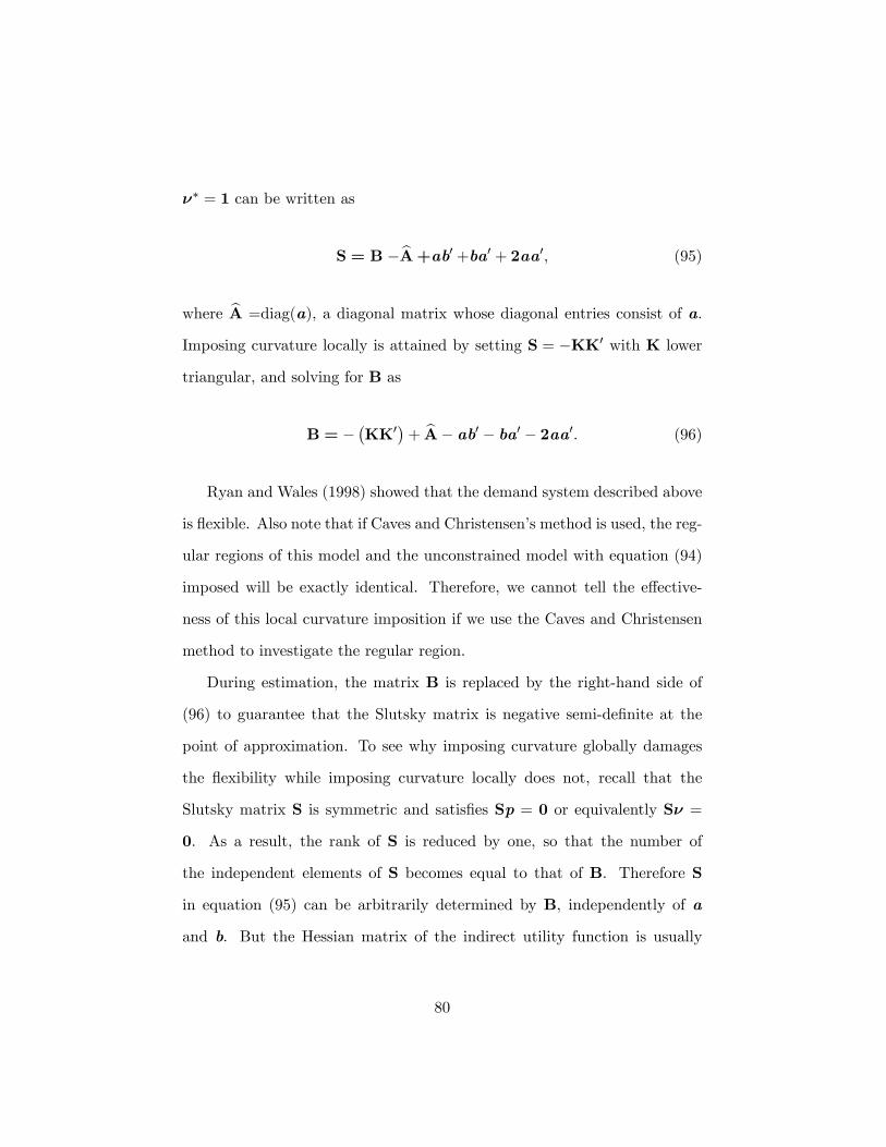
�� = 1 can be written as
S = B �bA+ab0 +ba0 + 2aa0; (95)
where bA =diag(a), a diagonal matrix whose diagonal entries consist of a.
Imposing curvature locally is attained by setting S = �KK0 with K lower
triangular, and solving for B as
B = ��KK0�+ bA� ab0 � ba0 � 2aa0. (96)
Ryan and Wales (1998) showed that the demand system described above
is �exible. Also note that if Caves and Christensen�s method is used, the reg-
ular regions of this model and the unconstrained model with equation (94)
imposed will be exactly identical. Therefore, we cannot tell the e¤ective-
ness of this local curvature imposition if we use the Caves and Christensen
method to investigate the regular region.
During estimation, the matrix B is replaced by the right-hand side of
(96) to guarantee that the Slutsky matrix is negative semi-de�nite at the
point of approximation. To see why imposing curvature globally damages
the �exibility while imposing curvature locally does not, recall that the
Slutsky matrix S is symmetric and satis�es Sp = 0 or equivalently S� =
0. As a result, the rank of S is reduced by one, so that the number of
the independent elements of S becomes equal to that of B. Therefore S
in equation (95) can be arbitrarily determined by B, independently of a
and b. But the Hessian matrix of the indirect utility function is usually
80

full rank unless linear homogeneity is imposed or attained empirically. In
Diewert andWales�(1988b) approach to prove the local �exibility, the second
partial derivatives at the point of approximation depend on both B and
a. However, imposition of non-negativity on a to attain global curvature
reduces the number of independent parameters and limits the span of B
and a. As a result, imposing curvature globally on this model damages
�exibility. Regarding local curvature imposition, the condition that the
Slutsky matrix be negative semi-de�nite is both necessary and su¢ cient for
correct curvature at the point of approximation.
3.3 Experimental Design
Our Monte Carlo experiment is conducted with a model of three demand
goods to permit di¤erent pairwise complementarities and substitutabilities.
The design of the experiment is described below.
3.3.1 Data Generation
The data set employed in the actual estimation process includes data for nor-
malized prices and budget shares, de�ned as � � p=x and w � bVq where qis a vector of demand quantities and bV is as de�ned previously. The data for
demand quantities are produced from the demand functions induced by two
globally regular utility functions: the CES functional form and the linearly-
homogeneous Constant-Di¤erences of Elasticities-of-Substitution (CDE) func-
tional form.33
33See Hanoch (1975), Jensen (1997), or section 2.2.1.1 for details of this model.
81
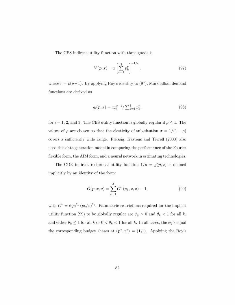
The CES indirect utility function with three goods is
V (p; x) = x
�3Pk=1
prk
��1=r; (97)
where r = �(��1). By applying Roy�s identity to (97), Marshallian demand
functions are derived as
qi(p; x) = xpr�1i =P3k=1 p
rk; (98)
for i = 1, 2, and 3. The CES utility function is globally regular if � � 1. The
values of � are chosen so that the elasticity of substitution � = 1=(1 � �)
covers a su¢ ciently wide range. Fleissig, Kastens and Terrell (2000) also
used this data generation model in comparing the performance of the Fourier
�exible form, the AIM form, and a neural network in estimating technologies.
The CDE indirect reciprocal utility function 1=u = g(p; x) is de�ned
implicitly by an identity of the form:
G(p; x; u) =3Xk=1
Gk (pk; x; u) � 1, (99)
with Gk = �ku�k (pk=x)
�k . Parametric restrictions required for the implicit
utility function (99) to be globally regular are �k > 0 and �k < 1 for all k,
and either �k � 1 for all k or 0 < �k < 1 for all k. In all cases, the �k�s equal
the corresponding budget shares at (p�; x�) = (1;1). Applying the Roy�s
82
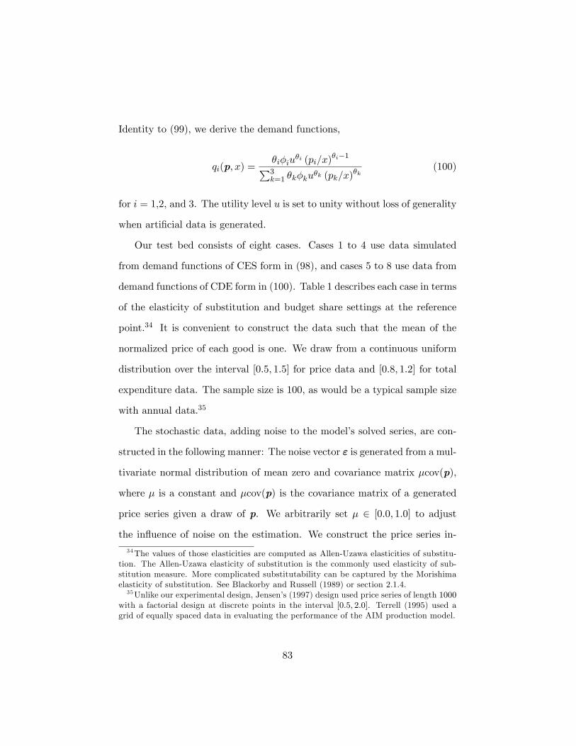
Identity to (99), we derive the demand functions,
qi(p; x) =�i�iu
�i (pi=x)�i�1P3
k=1 �k�ku�k (pk=x)
�k(100)
for i = 1,2, and 3. The utility level u is set to unity without loss of generality
when arti�cial data is generated.
Our test bed consists of eight cases. Cases 1 to 4 use data simulated
from demand functions of CES form in (98), and cases 5 to 8 use data from
demand functions of CDE form in (100). Table 1 describes each case in terms
of the elasticity of substitution and budget share settings at the reference
point.34 It is convenient to construct the data such that the mean of the
normalized price of each good is one. We draw from a continuous uniform
distribution over the interval [0:5; 1:5] for price data and [0:8; 1:2] for total
expenditure data. The sample size is 100, as would be a typical sample size
with annual data.35
The stochastic data, adding noise to the model�s solved series, are con-
structed in the following manner: The noise vector " is generated from a mul-
tivariate normal distribution of mean zero and covariance matrix �cov(p),
where � is a constant and �cov(p) is the covariance matrix of a generated
price series given a draw of p. We arbitrarily set � 2 [0:0; 1:0] to adjust
the in�uence of noise on the estimation. We construct the price series in-
34The values of those elasticities are computed as Allen-Uzawa elasticities of substitu-tion. The Allen-Uzawa elasticity of substitution is the commonly used elasticity of sub-stitution measure. More complicated substitutability can be captured by the Morishimaelasticity of substitution. See Blackorby and Russell (1989) or section 2.1.4.35Unlike our experimental design, Jensen�s (1997) design used price series of length 1000
with a factorial design at discrete points in the interval [0:5; 2:0]. Terrell (1995) used agrid of equally spaced data in evaluating the performance of the AIM production model.
83
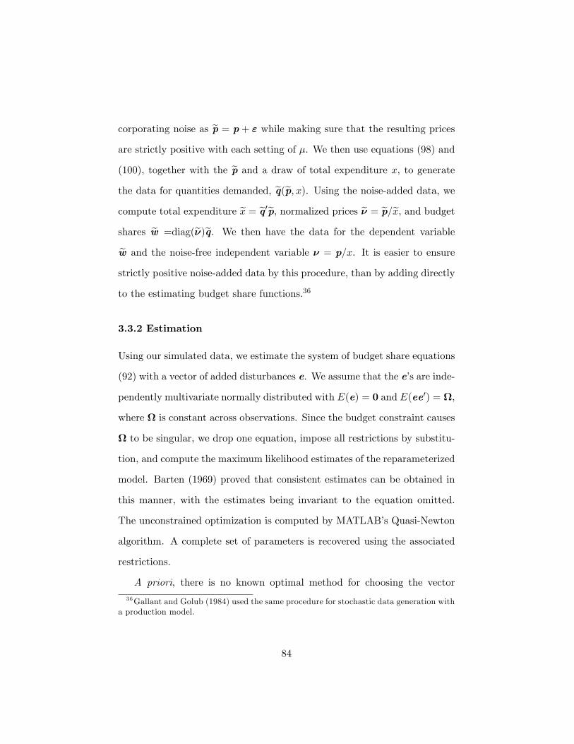
corporating noise as ep = p + " while making sure that the resulting pricesare strictly positive with each setting of �. We then use equations (98) and
(100), together with the ep and a draw of total expenditure x, to generatethe data for quantities demanded, eq(ep; x). Using the noise-added data, wecompute total expenditure ex = eq0ep, normalized prices e� = ep=ex, and budgetshares ew =diag(e�)eq. We then have the data for the dependent variableew and the noise-free independent variable � = p=x. It is easier to ensure
strictly positive noise-added data by this procedure, than by adding directly
to the estimating budget share functions.36
3.3.2 Estimation
Using our simulated data, we estimate the system of budget share equations
(92) with a vector of added disturbances e. We assume that the e�s are inde-
pendently multivariate normally distributed with E(e) = 0 and E(ee0) = ,
where is constant across observations. Since the budget constraint causes
to be singular, we drop one equation, impose all restrictions by substitu-
tion, and compute the maximum likelihood estimates of the reparameterized
model. Barten (1969) proved that consistent estimates can be obtained in
this manner, with the estimates being invariant to the equation omitted.
The unconstrained optimization is computed by MATLAB�s Quasi-Newton
algorithm. A complete set of parameters is recovered using the associated
restrictions.
A priori, there is no known optimal method for choosing the vector
36Gallant and Golub (1984) used the same procedure for stochastic data generation witha production model.
84
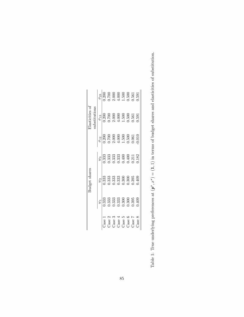
Budgetshares
Elasticitiesof
substitutions
w1
w2
w3
�12
�13
�23
Case1
0.333
0.333
0.333
0.200
0.200
0.200
Case2
0.333
0.333
0.333
0.700
0.700
0.700
Case3
0.333
0.333
0.333
2.000
2.000
2.000
Case4
0.333
0.333
0.333
4.000
4.000
4.000
Case5
0.300
0.300
0.400
1.500
1.500
1.500
Case6
0.300
0.300
0.400
0.500
0.500
0.500
Case7
0.395
0.395
0.211
0.061
0.561
0.561
Case8
0.409
0.409
0.182
-0.010
0.591
0.591
Table1:Trueunderlyingpreferencesat(p� ;x� )=(1;1)intermsofbudgetsharesandelasticitiesofsubstitution.
85
�, so we choose all elements of the vector to be equal. Some authors have
experimented with alternative settings, such as setting� as weights to form a
Laspeyres-like price index, but with no clear gain over our choice. Hence, all
elements of the vector � are set at 1=3 as a result of equation (91) with �� =
1.37 The number of Monte Carlo repetitions is 1000 for each case. We use
boxplots to summarize the distribution of the estimated elasticities across
the 1000 replicates. We follow the standard procedure for drawing boxplots.
The box has lines at the lower quartile, median, and upper quartile values.
The "whisker" is a line going through each end of the box, above and below
the box. The length of the whisker above and below the box equals 1:5�
(the upper quartile value � the lower quartile value). Estimates above or
below the whisker are considered outliers. Since we �nd these distributions
of estimates to be asymmetric, standard errors alone cannot capture what
is displayed in the boxplots. The average values of each parameter across
replications are used to produce the regular regions of the models.
To begin our iterations, we start as follows: We compute the gradient
vector and the Hessian matrix of the data-generating function at the point
(p�; x�) = (1;1). We set that vector and that Hessian of the Normalized
Quadratic model to be the same as those of the data generating model
at that point. We then solve for corresponding parameter values of the
Normalized Quadratic model and use the solution as the starting values for
the optimization procedure. Those starting parameter values produce a local
second order approximation of the Normalized Quadratic to the generating
function. Our starting values facilitate convergence to the global maximum
37See Kohli (1993) and Diewert and Wales (1992).
86
of the likelihood function, since the global maximum is likely to be near the
starting point.
3.3.3 Regular Region
Following Jensen (1997), we plot two-dimensional sections of the regular re-
gion in the Cartesian plane. The x-axis represents the natural logarithm of
(p2=p1), and the y-axis the natural logarithm of (p3=p1). Each axis ranges
between ln(0:2=5:0) � �3:2189 and ln(5:0=0:2) � 3:2189. The sample range
is de�ned as the convex hull of possible prices within the above intervals of
relative values and is displayed in our �gures as a rectangle in the center of
the graph. Accordingly, each of the four sides of the rectangle range from
ln(0:5=1:5) � �1:0986 to ln(1:5=0:5) � 1:0986 since our data is generated
from the interval of [0:5; 1:5]. The entire section is divided into 150 � 150
grid points at which the monotonicity and curvature conditions are evalu-
ated. Each plot can be viewed as a display of a two-dimensional hyperplane
through the three-dimensional space having dimensions ln(p2=p1), ln(p3=p1),
and ln(x). We section the regular region perpendicular to the ln(x) axis at
the reference point of x = 1:0. It is desirable to plot several hyperplanes
at di¤erent settings of x, as done by Barnett, Lee and Wolfe (1985, 1987)
to investigate the full three-dimensional properties of the model�s regular
region. But, since regularity is usually satis�ed at the reference point and
violations increase as data points move away from the reference point, the
emergence of regularity violations on the single hyperplane with x �xed at
the reference setting is su¢ cient to illustrate de�ciencies of the Normalized
Quadratic Model.
87
The monotonicity condition is evaluated using the gradient vector of the
estimated equation in (89), rV (�). The model is required by theory to
be strictly increasing in �. For each grid point at which the gradient is
evaluated, the monotonicity condition is satis�ed, if rV > 0.
Our approach to evaluation of the curvature condition di¤ers from that
used in most studies. In those other studies, the curvature condition is
judged to be satis�ed if the Allen elasticity of substitution matrix or the
Slutsky substitution matrix is negative semi-de�nite.38 The problem is that
satisfaction of the monotonicity condition is required for those matrix con-
ditions to be necessary and su¢ cient for satisfaction of the curvature condi-
tion. Hence, we do not use substitution matrices to evaluate the curvature
condition. We directly evaluate the quasiconcavity of the equation (89) us-
ing the method proposed by Arrow and Enthoven (1961). Quasiconcavity
is checked by con�rming alternating signs of the principal minors of the
bordered Hessian matrix, which contains the second partial derivatives bor-
dered by �rst derivatives.39 This approach is general, regardless of whether
there are any monotonicity violations.
Each grid is �lled with di¤erent gradations of black and white, designat-
ing the evaluation results for the regularity conditions. The completely black
grid designates violations of both curvature and monotonicity; the very dark
grey grid designates violation of only curvature; and the very light grey grid
speci�es violation of only monotonicity. The completely white regions are
38For example, Serletis and Shahmoradi (2005) computed the Cholesky values of theSlutsky substitution matrix to evaluate its negative semi-de�niteness. A matrix is negativesemi-de�nite, if its Cholesky factors are non-positive (Lau, 1978).39The procedure is described in detail in section 2.1.5.
88
fully regular. There are 8 cases with 3 models each, resulting in 24 plots of
regular regions.
3.4 Results and Discussion
We con�rm convergence to a global maximum of the likelihood function by
comparing the estimated elasticity values with the true ones. If the discrep-
ancy is large, we discard that run and rerun the program. We do not seek to
explain the cases of large discrepancies, other than to conclude that under
such circumstances, an unresolved problem exists. Based on this criterion,
we encounter substantial di¢ culty in the estimation of the model with local
curvature imposed. When data are generated with elasticities of substitu-
tion greater than unity (cases 3, 4 and 5), the estimates converge to values
far from the true ones. But when we try the somewhat lower elasticities
of �12 = �13 = �23 = 1:10 or 1:20, convergence to reasonable estimates
is more successful although some replications still often yield unreasonable
estimates.
The boxplots of case 4 in �gure 1 describe the distributions of 1000 esti-
mates of the elasticities of substitution by the models with no curvature im-
posed (left), local curvature imposed (middle), and global curvature imposed
(right).40 The estimates of the elasticities from the local curvature imposed
model not only have larger variations (described as longer whiskers) than
those from the no curvature imposed and global curvature imposed models,
but also include a number of severe outliers especially in the positive direc-
40All data used for boxplots are generated with � = 0:20 for the noise adjustmentconstant.
89
tion. Even when estimates of cross elasticities are reasonable, estimates of
the own elasticities were often found to be far from the true values. In fact,
the unconstrained and global-curvature-imposed models both require very
high values of a (around 400; 000�s to 600; 000�s for all elements) to attain
maximization of the likelihood function. We suspect that constraint (94)
is too restrictive. For the local-curvature-imposed model to approximate
a symmetric function, as in cases 3 and 4, the optimal values of a should
all be zeros while satisfying the restriction (94). However, any statistical
tests would reject the hypothesis that the restriction is valid. Moreover, as
Diewert and Wales (1988b) observed, equation (94) often renders global con-
cavity to be impossible. The only way to achieve globally correct curvature
with (94) is to set a = 0, since global concavity requires non-negativity of
all elements of a. In addition, since B is a function of a as well as of b and
K, any poor estimate of a will produce poor estimation of B which contains
a set of parameters that explain the model�s curvature property. With all
such problems and nonlinearity embedded in the likelihood function, the
optimization algorithm can search for wrong local maxima. We tried a few
global optimization techniques, but without success.41 When the point esti-
mates of elasticities are themselves poor, we view regularity violations to be
a "higher order problem" of lesser concern. For reference purposes, we plot
in �gure 2 the regular region of the local curvature imposed model (top)
along with that of the global curvature imposed model (bottom). However,
41The genetic algorithm and the pattern search method were tried. But the lack ofconvergence of the former and the very slow convergence of the latter is a substantialcomputational burden for any study that requires a large number of repeated simulations.Dorsey and Mayer (1995) provide an empirical evaluation in econometric applications ofthe performance of genetic algorithms versus other global optimization techniques.
90
the validity of conclusions drawn from that �gure is questionable.
A display of the regular region of the model with global curvature im-
posed (bottom) in �gure 2, the regularity violations occupy a large part of
the area. Within the very light grey areas of the plots, the regularity vio-
lations are attributed entirely to monotonicity violations. Severe regularity
violations resulted from using data produced with high elasticities of sub-
stitution, and therefore, the most severe violations occurred in case 4. The
plot of case 3 displays similar shape of regularity violation regions to case
4, but with a somewhat wider regular region. In case 4, we obtained an
almost identical �gure with the unconstrained model. Regularity violations
indued by the monotonicity violations may indeed be common with many
nonglobally regular �exible functional forms and should not be viewed as
exclusive to the Normalized Quadratic model.
In case 4, the model substantially underestimates true elasticities. The
boxplot (right) in �gure 1 shows that the median of the 1000 sample es-
timates is near 3:0, while the true elasticity is 4:0. This �nding is similar
to those of Guilkey, Lovell and Sickles (1983) and Barnett and Lee (1985),
which showed that the generalized Leontief model performs poorly when
approximating the function with high elasticities of substitution. We �nd
that the Normalized Quadratic model performs poorly both in estimating
elasticities and in maintaining regularity conditions when the data used was
produced with high elasticities of substitution.
For cases 1, 2, and 6, all models perform very well with no regularity
violations. The Normalized Quadratic model performs well when the data is
characterized by low elasticities of substitution (below unity) and pairwise
91
elasticities are relatively close to each other. The plot with case 5 is omitted
since the result is similar to case 4.42
With case 7, the plot on the top in �gure 3 displays a very dark grey
cloud on the top-right part of the plot, designating curvature violations for
the unconstrained model. In this case, imposing curvature locally as well as
globally eliminates all of the curvature violations within the region of the
data, as shown by the entirely white region in the bottom plot. Figure 4
describes the distributions of estimates in case 7. For all three models, the
median estimates are satisfactorily close to true elasticities. With global
curvature imposed, elasticity estimates are severely downward-biased when
the true elasticities are high, and upward-biased when the true elasticities
are low as outliers. This suggests that all pairwise elasticities become close
to each other. As should be expected by the outliers, the cause is not easy to
determine, and we do not impute much importance to results with outliers.
These problems do not arise when we impose curvature locally in case 7 in
which the local curvature imposition succeeds in producing global regularity
within the region of our data.
Figure 5 displays plots for case 8 of the regular regions for the uncon-
strained model (top) and the local-curvature constrained model (bottom).
The top of the upper plot has a wide, thick cloud of curvature violations.
That region intersects a small monotonicity-violation area on the right side.
42With case 5 there are regularity violations inside the sample range as in case 4, butto a milder extent, as in case 3, since both case 3 and 5 use data with lower elasticities ofsubstitutions than case 4. The plot of case 5 is slightly shifted from the center as a resultof the fact that the simulated budget shares at the center point are slightly asymmetric.The plot is very similar to the case I of Jensen (1997). Our case 5 and his case I use thesame data-generating setting.
92
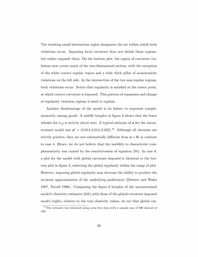
The resulting small intersection region designates the set within which both
violations occur. Imposing local curvature does not shrink those regions,
but rather expands them. On the bottom plot, the region of curvature vio-
lations now covers much of the two-dimensional section, with the exception
of the white convex regular region and a wide thick pillar of monotonicity
violations on the left side. In the intersection of the two non-regular regions,
both violations occur. Notice that regularity is satis�ed at the center point,
at which correct curvature is imposed. This pattern of expansion and change
of regularity violation regions is hard to explain.
Another disadvantage of the model is its failure to represent comple-
mentarity among goods. A middle boxplot in �gure 6 shows that the lower
whisker for �12 is strictly above zero. A typical estimate of a for the uncon-
strained model was a0 = (0:014; 0:014; 0:262).43 Although all elements are
strictly positive, they are not substantially di¤erent from a = 0, in contrast
to case 4. Hence, we do not believe that the inability to characterize com-
plementarity was caused by the restrictiveness of equation (94). In case 8,
a plot for the model with global curvature imposed is identical to the bot-
tom plot in �gure 3, achieving the global regularity within the range of plot.
However, imposing global regularity may decrease the ability to produce the
accurate approximation of the underlying preferences (Diewert and Wales
1987, Terrell 1996). Comparing the �gure 6 boxplot of the unconstrained
model�s elasticity estimates (left) with those of the global-curvature imposed
model (right), relative to the true elasticity values, we see that global cur-
43The estimate was obtained using noise-free data with a sample size of 500 instead of100.
93

vature imposed model overestimates the elasticity of substitution, �12, for
complementarity and the elasticities of substitution, �13 and �23 for substi-
tutes. A possible cause is the imposition of negative semi-de�niteness on
the Hessian matrix. As in �gure 4 the outlier estimates cause the pairwise
elasticities of substitution estimates to become closer to each other.
3.5 Conclusion
We conducted a Monte Carlo study of the global regularity properties of
the Normalized Quadratic model. We particularly investigated monotonic-
ity violations as well as the performance of methods of locally and globally
imposing curvature. We found that monotonicity violations are especially
likely to occur when elasticities of substitution are greater than unity. We
also found that imposing curvature locally produces di¢ culty in the estima-
tion, smaller regular regions, and the poor elasticity estimates in many of
the cases considered in this chapter.
When imposing curvature globally, our results were better. Although
violations of monotonicity remain common in some of our cases, those viola-
tions do not appear to be induced solely by the global curvature imposition,
but rather by the nature of the Normalized Quadratic model itself. However,
imposition of global curvature does induce a problem with complementary
goods by biasing the estimates towards over complementarity and substitute
goods towards over substitutability.
With the Normalized Quadratic model, we �nd that both curvature and
monotonicity must be checked with the estimated model, as has previously
been shown to be the case with many other �exible functional forms. Im-
94

position of curvature alone does not assure regularity, and imposing local
curvature alone can have very adverse consequences.
95
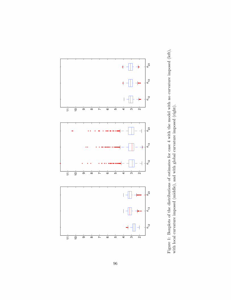
Figure1:Boxplotsofthedistributionsofestimatesforcase4withthemodelwithnocurvatureimposed(left),
withlocalcurvatureimposed(middle),andwithglobalcurvatureimposed(right).
96

log(p2/p1)
log(
p 3/p1)
log(p2/p1)
log(
p 3/p1)
Figure 2: Section through regular regions of the model at x = 1:0 with localcurvature imposed (top) and with global curvature imposed (bottom) forcase 4.
97
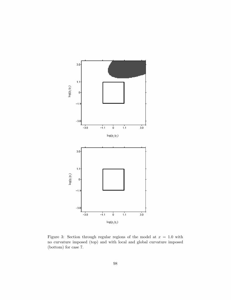
log(p2/p1)
log(
p 3/p1)
log(p2/p1)
log(
p 3/p1)
Figure 3: Section through regular regions of the model at x = 1:0 withno curvature imposed (top) and with local and global curvature imposed(bottom) for case 7.
98
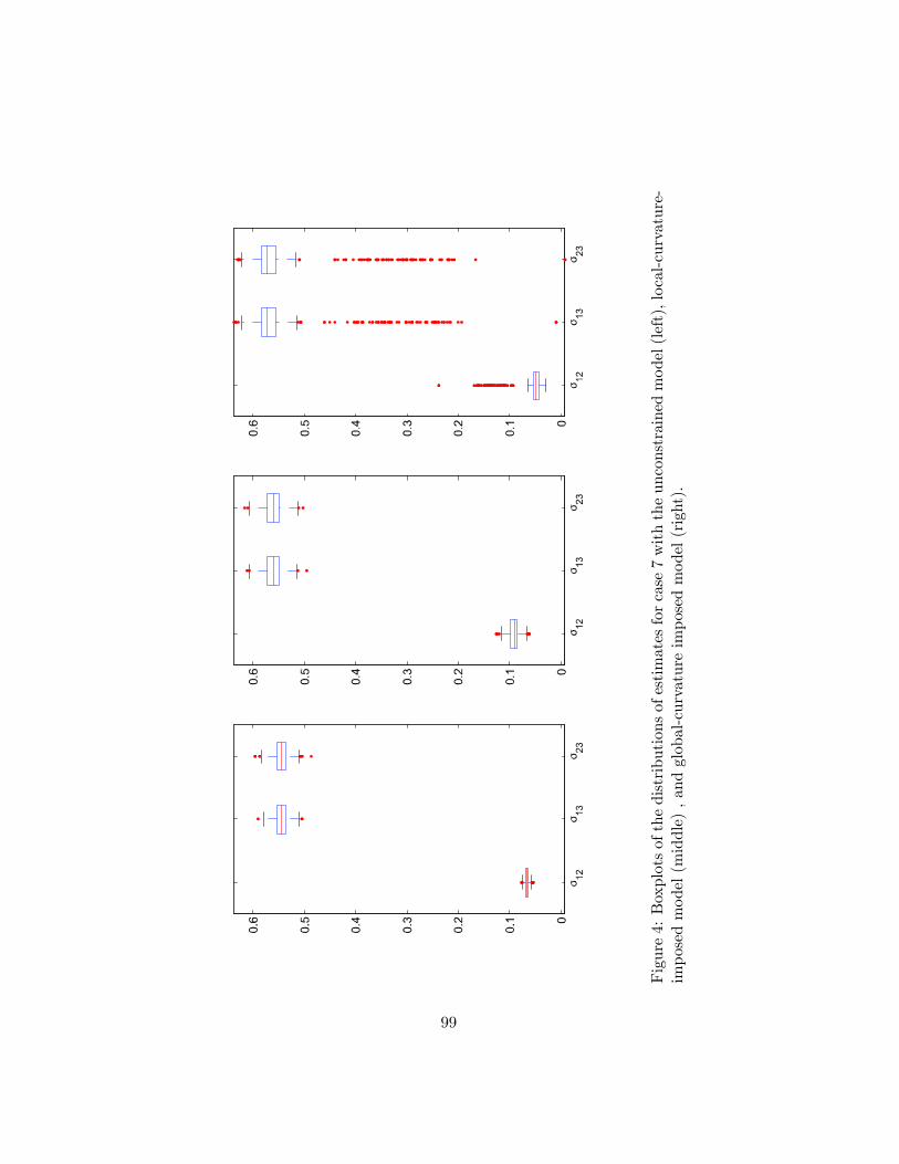
Figure4:Boxplotsofthedistributionsofestimatesforcase7withtheunconstrainedmodel(left),local-curvature-
imposedmodel(middle),andglobal-curvatureimposedmodel(right).
99
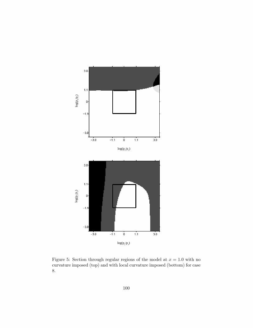
log(p2/p1)
log(
p 3/p1)
log(p2/p1)
log(
p 3/p1)
Figure 5: Section through regular regions of the model at x = 1:0 with nocurvature imposed (top) and with local curvature imposed (bottom) for case8.
100
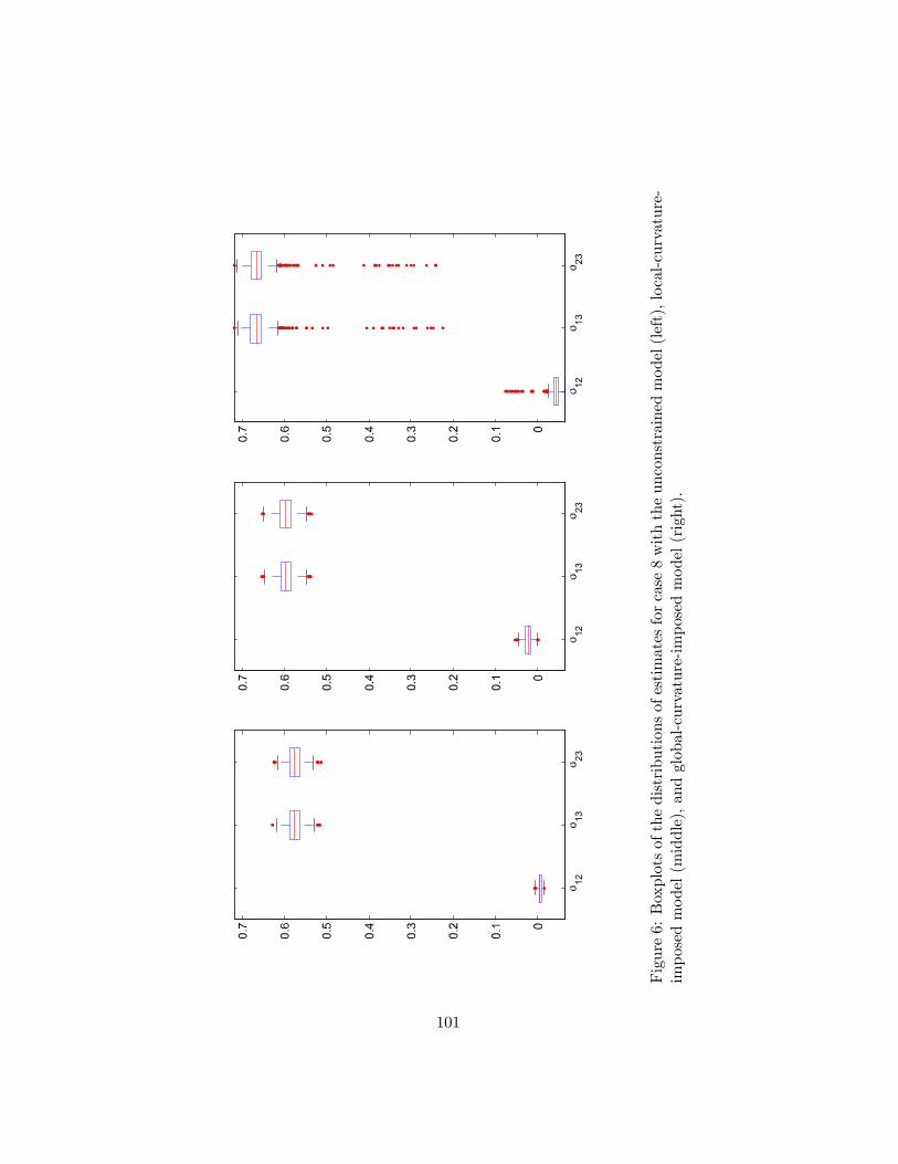
Figure6:Boxplotsofthedistributionsofestimatesforcase8withtheunconstrainedmodel(left),local-curvature-
imposedmodel(middle),andglobal-curvature-imposedmodel(right).
101
Chapter 4
Estimation of Expenditure-Dependent Equivalence Scales and the
Cost of a Child Using Japanese Household Expenditure Data
4.1 Introduction
This empirical section demonstrates the use of rank three and rank four
consumer demand models which can characterize more complicated Engel
curve shapes, and it investigates household consumption behaviors using
household expenditure survey data, especially for attempts to estimate the
cost of a child using Japanese household expenditure data. An Engel curve
is the function describing how consumer�s expenditures on some goods or
services relate to her total expenditure while keeping prices �xed. The rank
of a demand system can be de�ned as the dimension of the space spanned
by its Engel curves. A famous result by Gorman (1981) tells that exactly
aggregable demand systems have at most rank three or less. Lewbel (1991)
extended Gorman�s result and de�nes the rank M of any demand system
to be the maximum dimension of the function space spanned by the Engel
curves of the demand system.
We employ a rank three demand system of QUAIDS (Bank, Blundell
and Lewbel, 1997) and a rank four demand system of translated QUAIDS
(Lewbel 2003; Donaldson and Pendakur 2006) in this chapter for empirical
parametric speci�cations of demand models. Given the large set of house-
hold expenditure data within which observations of total expenditure vary
substantially, higher rank demand systems are necessary tools to account for
102
the observed expenditure patterns at di¤erent income levels than the lower
rank, say, rank two demand systems such as models of the PIGLOG type
which are linear in logarithm of total expenditure.44 For analyses involving
only a modest range of income levels, such richness in global Engel curve
shapes may be unnecessary, just as local �exibility (in Diewert�s sense) may
adequately capture a full range of price e¤ects when prices do not change
much over a sample. However, income levels usually vary widely across
households, and analysis of welfare or cost-of-living involves comparisons
of demands between these income levels. So, in studies involving cross-
sectional data, cost-of-living analyses, or welfare comparisons, richness in
Engel curve shapes across a wide range of income level is required. The re-
sults of nonparametric kernel regressions of Engel curves for UK households
(Bank, Blundell and Lewbel, 1997) showed that the linear relationship is
not su¢ cient to characterize the shape of the Engel curves on some goods
which exhibit nonlinear shapes of Engel curves. The nonparametric rank
test (Gill and Lewbel 1992; Gragg and Donald, 1997) also suggested that a
rank three relationship is required, as would be the case in the second-order
polynomial. Blundell, Chen and Kristensen (2007) found that some goods
have Engel curves that are close to linear or quadratic, while others are more
S-shaped.
There are a number of studies which concern the rank of demand sys-
tems, and a number of tests of rank have been conducted either paramet-
rically, semiparametrically or nonparametrically (Grodal and Hildenbrand
44The AIDS model, which has rank two, performed poorly in the Monte Carlo study ofBarnett and Seck (2007) using several linear approximation methods.
103
1992; Hildenbrand 1994; Kneip 1994; Lewbel 1991; Donald 1997; Hausman,
Newey and Powell 1995; and Lyssiotou, Pashardes and Stengos 1999). Nicol
(2001) �nds that conditional demands for some demographic groups are
rank three, which implies that unconditional demands for those groups are
likely to be rank four. Lyssiotou, Pashardes and Stengos (2008) suggest the
possibility of higher rank than three.45
Therefore, contemporary studies on household demand behaviors are
expected to adopt at least rank three demand systems if no (nonparametric)
rank test is carried out or no knowledge about the shape of its Engel curves
is available a priori. The rank three parametric demand system used almost
exclusively is the quadratic AIDS model. It nests a classic AIDS model,
and hence, provides a simple way to test against the speci�cation of the
additional quadratic term. The linearization method for QUAIDS, as for
AIDS, is also made available by Matsuda (2006) to help ease the complicated
nonlinear estimation.
Lewbel (1991) showed that a class of de�ated income demand systems
which has Engel functions as being a function of "de�ated" income which is
the total expenditure divided by some homogeneous of degree one function
of prices, can have rank up to four. In fact, the classic AIDS and QUAIDS
are members of this class, as can be seen by their form.46 Lewbel (2003)
and Donaldson and Pendakur (2006) speci�ed the four price functions of
a rank four de�ated income demand system and estimated the household
demands using the UK Family expenditure survey and the Canadian Family
45See Lewbel (2002).46See section 2.2.5.8.
104
Expenditure Surveys, respectively. The model replaces x in QUAIDS with
x�d(p), where d(p) is a "translation" function and is homogeneous of degree
one in prices to maintain the homogeneity of the original QUAIDS. This
method of introducing translation or overhead term into demand systems
is well known (see Samuelson, 1948; and Gorman, 1976), and typically has
the e¤ect of increasing the rank of the demand system. The system is called
"translated" QUAIDS by Donaldson and Pendakur (2006). The rank four
model allows one to test for the speci�cation of rank three.
Having speci�ed the model of demand functions, one needs to consider
how to incorporate the demographic characteristics into the individual con-
sumer demand model to represent di¤erent types of households. Lewbel
(1985) provided a general approach to do this by modifying the expenditure
function through two modifying functions. This method leads to the rep-
resentation that the welfare level (or utility) of the households with some
characteristics is equal to the utility level of a reference household with in-
come and prices adjusted through these modifying functions. We show that
the particular speci�cations of the demographic modi�cation give rise to
the equivalent-expenditure functions which are used to conduct the welfare
analysis. The equivalent-expenditure function depends on prices and house-
hold characteristics, and is that expenditure which, if enjoyed by a reference
household facing the same prices, would result in a utility level equal to
that of each household member. The equivalence scales are the ratio of
expenditure to equivalent expenditure (relative) or the di¤erence between
expenditure and equivalent expenditure (absolute).
We limit our attention to the identi�able equivalent-expenditure func-
105
tions (and equivalence scales) by demand data alone. Equivalent-expenditure
functions and equivalence scales are identi�able by demand data if there is
a one-to-one correspondence between the preference ordering and the ob-
served demands which it generates.47 This identi�cation requires either
strong, untestable assumptions regarding preferences or unusual types of
data. Our identi�cation focuses on imposing as little restriction as possible
on the household preference structure.
Lewbel (1989) and Blackorby and Donaldson (1993) consider the case
where the equivalence scale function is independent of utility, which they call
"independence of base" (IB) and "equivalence-scale exactness (ESE), respec-
tively.48 The ESE property assumes that household expenditure functions
across families with di¤erent demographic compositions are proportional
with respect to reference expenditure, hence equivalence scales are, a priori,
independent of reference income. Blackorby and Donaldson (1993) showed
that the exact equivalence scales are identi�ed by observed demand data
if the preference of the reference household is not PIGLOG (not log-linear
in utility). This is an unfortunate result because PIGLOG speci�cation
includes the popular AIDS model of Deaton and Muellbauer and exactly
aggregable translog of Jorgenson, Lau and Stoker (1982). Despite the identi-
�ability and convenience of econometric approaches, exact equivalence scales
may not hold in practice, due to the restrictive form of household prefer-
ences that they impose, as can be found in the later section. Tests of the
47For a detailed explanation of the identi�ablility of equivalence scales, see Pollak andWales (1979), Blundell and Lewbel (1991), Lewbel and Pendakur (2006). A more technicalpresentation is given by Blackorby and Donaldson (1991, 1993), Lewbel (1989d).48We use the term of Blackorby and Donaldson in this dissertation.
106
exactness of equivalence scales have produced mixed results.49
Exact equivalence scales have a critical disadvantage for policy purposes
as well as for economic interpretation. Conni¤e (1992) argues that equiva-
lence scales are not constant as regards income and that the current prac-
tice of assuming the exactness of equivalence scales should be reconsidered.
Koulovatianos, Schröder and Schmidt (2005) �nds strong evidence from re-
search surveys conducted in Germany and France that equivalence scales are
signi�cantly decreasing in reference income, and strongly encourage the use
of parametric or semi-parametric demand systems that can produce equiv-
alence scales which are decreasing in reference income. Yet scales used in
comparative and policy-related welfare studies have almost always used the
exactness property of equivalence scales. The exact equivalence scales sug-
gest that a rich household with a child has higher equivalent expenditures
than a poor household with a child since exact equivalent expenditures are
proportional to the reference income of that particular household without a
child. No researcher or policy-maker seriously suggests that within a par-
ticular society higher income groups should be deliberately granted greater
monetary compensation for having children (through child allowances, or
whatever) than lower income groups. In the formulation of policy in the
areas of welfare bene�ts and tax allowances, the assumption of exact equiv-
alence scales could have serious and unacceptable implications.
49See Blundell and Lewbel, 1991, Dickens, Fry and Pashardes 1993, Pashardes 1995,Blundell, Duncan and Pendakur 1998, Gozalo 1997, Pendakur 1999, Koulovatianos,Schroder and Schmidt 2005. Semi- or non-parametric speci�cation of demand systemstends to satisfy the equivalence-scale exactness, suggesting that the validity of the ESEcondition may be attributed to the parametric speci�cations of the demand system. Alsonote that it is possible to statistically reject ESE, but if the the demand restrictions impliedby ESE are not rejected, it remains impossible to infer that ESE actually holds.
107
An approach to relax the exact equivalence scales is suggested by Don-
aldson and Pendakur (2004). In particular, they introduce a property named
"Generalized Relative Equivalence Scale Exactness "(GRESE) which implies
a linear relationship between the log of equivalence scales and the log of ref-
erence incomes. Therefore, if the slope of this linear relationship is negative
with a positive intercept term, then the equivalence scales are consistent
with the recommendation of Koulovatianos, Schröder and Schmidt (2005).
They show that if GRESE is a maintained hypothesis and the reference
expenditure function is not PIGLOG, the equivalent-expenditure function
can be identi�ed from demand behavior. Since GRESE nests ESE, the es-
timation of demand systems allows for an easy speci�cation test for a more
appropriate equivalence scale structure.
Donaldson and Pendakur (2006) also relax the exact "absolute" scales
and name the property "Generalized Absolute Equivalence Scale Exactness
(GAESE) which implies a linear relationship between the equivalence scales
and the reference incomes. GAESE allows for formulation of the equivalent-
expenditure functions with a �xed component and a variable component
that is proportional to the reference income.
We use the Japanese Panel Survey on Consumers (JPSC) conducted and
administered by the Institute for the Research on Household Economics for
household expenditures and characteristics data. Estimation of child cost in
Japan itself is an interesting subject in the context of the super-low fertility
rate of Japan. In addition, discussion of a child subsidy program became one
of the biggest political hooking points during the recent general elections,
which took place in the summer of 2009. Despite the evidence documented
108
by Koulovatianos, Schröder and Schmidt (2005), it may not be evident that
the equivalence scales are decreasing in the income given seemingly gener-
ous existing child-suppot welfare programs because the universally available
medical insurance in Japan may lesson the out-of-pocket cost of additional
children compared to the U.S., where a large number of households do not
have any medical insurance (Phipps and Garner, 1994). The discussion on
the low fertility trend in Japan and the ongoing discussion of child-support
programs is placed in the next section.
We have encountered the existence of a mass of zero-expenditure ob-
servations for some of the goods in our data set. With the presence of a
large pile of budge share observations at zero, the usual estimation proce-
dure of appending a normal error vector to the demand system to solve the
nonlinear simultaneous system of equations becomes di¢ cult to apply. It
makes the distribution of error terms hardly look normal, and the resulting
parameter estimates become biased. There are several methods to deal with
the zero expenditure issue, depending on what kind of underlying causes
are expected to be generating zero expenditures. We assume that the un-
derlying cause is the infrequent purchase of goods (IFP). 50 Although the
commodities are actually consumed, purchases may not be recorded because
the purchase interval is longer than the survey period. We believe that this
is an appropriate assumption in wealthy countries like Japan, as opposed to
developing countries where many households do not purchase certain goods
because they are too expensive. We adopted the Amemiya-Tobit approach,
speci�cally, a variant of Heckman�s (1979) sample selection model in which
50See Deaton and Irish (1982).
109

the consumer decides to purchase a good based on some exogenous vari-
ables other than prices and income, and then allocates her budget to decide
how much to purchase. We estimated the model using a two-step proce-
dure proposed by Shonkwiler and Yen (1999) that consists of the �rst step
of the Probit estimations of each equation, which determines the purchase
decision, and the second step of estimating the augmented demand system,
based on the parameter estimates obtained from the �rst step.
We �nd that the GRESE speci�cation with the QUAIDS preferences
of the households is statistically preferred to any of the more restricted
speci�cations and that the equivalence scales are negatively correlated with
the total expenditure levels. The results are appealing since the equivalence
scales are identi�ed by rejecting AIDS speci�cation which is PIGLOG, and
hence, there is no ambiguity with the result in that sense. Moreover, the
implication is that the equivalence scales increase (decrease) as the total
expenditures decrease (increase), which is consistent with the �ndings of
Koulovatianos, Schröder and Schmidt (2005) and Conni¤e (1992). It gives
the straightforward policy design implication that poor households should be
more compensated than rich households when they have additional children
if a child-support policy is pursued by the Japanese government at all.
This chapter is organized as follows: Section 2 presents the current dis-
cussion on the low birthrate trend in Japan and the public policies that
are designed to tackle this issue. Section 3 shows how to construct the de-
mographically modi�ed expenditure function using Lewbel�s (1985) proce-
dure. Section 4 shows the de�nition of equivalence scales and ESE property,
and it presents two types of characterizations of Donaldson and Pendakur�s
110
equivalent-expenditure function. Section 5 describes our empirical paramet-
ric model speci�cation including the construction of our datasets. Section
6 describes the estimation procedure with emphasis on how to deal with a
piled-up of expenditure observations at zero in the data. Section 7 presents
the results, and the conclusion follows.
4.2 Discussion on Low Fertility Rate, Relevant Public Policies, andEmpirical Equivalent Scales in Japan
Japan has been recording very low fertility rates over the years, 1.27 as of
2009.51 Although South Korea now has the lowest fertility rate, 1.22, the
low fertility rate is more problematic for Japan in view of the fact that Japan
is the "oldest"country meaning that the median age of the whole population
is the highest among all countries (44.4 years old). The dependency ratio,
an age-population ratio of those typically not in the labor force (the depen-
dent part) and those typically in the labor force (the productive part) has
increased to 22.7 in 2009 whereas it was 4.9 in 1950. Therefore, this pro-
longed low birthrate level creates an unbalanced demographic composition
between productive and dependent populations. This trend may result in
a greater burden per person regarding social security and have a negative
e¤ect on Japan�s long-term economic performance.
There are several government programs that have existed and have been
expanded in response to the declining trend of birthrate. The child subsidy
program (Jidouteate) is de�nitely one of the most important of the policies
designed to help families with child-rearing expense. Japanese households
51See Date and Shimizutani (2007) for the up-to-date survey paper on the cause of thedeclining fertility rate of Japan written in English.
111
currently (as of 2009) receive 5,000 or 10,000 yen per child with the cuto¤
amount dependent upon household income level and the age of the children.
Beginning in 1993, the amount of allowance which applied to children under
three years of age was 5,000 yen each for a �rst and second child, and 10,000
yen for each additional child. In 2000, the age cuto¤ increased to 6 years
of age (or before attending elementary school age), and the amount for all
children under 3 years of age increased to 10,000 yen in 2007, even for a �rst
or second child. After April 2006, the cuto¤ income level for national health
insurance holders, for instance, starts at 4,600,000 yen and increases by
380,000 yen each as the number of dependent household members increases.
In October 2006, to o¤set medical expenses incurred from childbirth, the
one-time government allowance paid to families with newborn children was
increased from 300,000 yen to 350,000 yen, and to 420,000 yen in October
2009. Tanaka and Kouno (2009) found that an increase of 100,000 yen in the
one-time government childbirth allowance raises the fertility rate by 0.017.
A tax credit for dependent family members also helps decrease the cost of
raising children. An income tax credit of 380,000 and a residential tax credit
of 330,000 yen per dependant are given as of 2009. The dramatic increase
in the amount of child support allowance proposed as a new child subsidy
program by DPJ (Minshuto) was one of the biggest issues debated during the
general election campaign in Japan prior to the the election held on August
30, 2009. The party currently holding the cabinet o¢ ce is advocating the
allowance amount of 26,000 yen per child younger than 15 year of age (or
junior highschoolers) without an income threshold. The issue of no income
threshold has been controversial in the current policy debate.
112
Despite the seemingly generous monetary compensation o¤ered by the
government welfare program to compensate for child-birth and child-rearing
expenses, when couples are asked the reason why their planned number of
children is lower than their preferred number of children, the majority re-
ports that cost is the major issue. According to the latest Thirteenth Basic
Survey on Birth Trend, 65.9% of couples report that "child-rearing and edu-
cation costs are too high."52 Therefore, it is of particular interest to see how
the obtained equivalence scales are compared to scales found in other studies
using di¤erent data sets and to see if the result of the Basic Survey on Birth
Trend is consistent with the scales obtained from the estimation results.
The papers that actually calculated the equivalence scales include Nagase
(2001), Suruga (1993, 1995), and Suruga and Nishimoto (2001). They all
used Engel or Rothbarth methods which impose very restricted assumptions
on preferences and equivalence scales.53 Oyama (2006) used psychometric
data in the form of an Income Evaluation Question to estimate the equiva-
lence scales.54 She found that the cost of a child aged 0-18 years is between
1:386 and 1:475; between 1:280 and 1:454 for a child aged 0-6; between 1:277
to 1:407 for the age range 7-13 years; and between 2:090 to 4:329 for the
age range 14-18. Recently, Hasegawa, Ueda and Mori (2008) undertook es-
timation of equivalence scales with the system of Working-Lesser equations
52The source for this information is the National Institute of Population and SocialSecurity Research, Dai 12 kai shussei doukou kihon chousa [Thirteen Basic Survey onBirth Trends] (www.ipss.go.jp).53The Rothbarth method using the consumption pattern of adult goods requires sep-
arability assumption between the parents�and the children�s consumption. See Gronau(1988) and Nelson (1992).54See Van Praag and Warnaar (2003) Van Praag and Kapteyn (1973), and Van Praag
and Van der Sar, (1989).
113
using the same data source as ours. They produced an equivalence scale of
1:3695.
Other studies related to this topic include Matsuura (2007), who �nds
that the marginal utility of having children is higher for males in the con-
text of the hypothesis that education cost is a major cause of reluctance to
have more children. Aoki and Konishi (2009a, 2009b) show that improved
quality of consumption has a negative impact on the birthrate in relation to
female labor supply. Abe (2005) studied the e¤ects of child-related bene�ts
and found that these bene�ts contribute little to the reduction of poverty
in households with children. Yamaguchi (2005a, 2005b, 2006) provides a
sociological view of how the society overall can help raise the fertility rate.
4.3 Demographically Modi�ed Demand System
Lewbel (1985) proposed a uni�ed approach to incorporate demographic ef-
fects into any demand systems. His method generalizes the existing ap-
proaches of demographic translating, demographic scaling (Barten scale),
and the modi�ed Prais-Houthakker procedure (Pollak andWales 1981, 1992).
It o¤ers a large class of possible modi�cations that have both the universal
applicability of demographic scaling and translating, and the �exibility to
allow demographic variables to interact with price and expenditure terms in
the demand system in an almost unlimited variety of ways.
Lewbel�s procedure modi�es the expenditure function by �rst replacing
each price by a function that depends on all prices and demographic variables
and then subjecting the resulting expenditure function to a further trans-
formation that depends on all price and demographic variables. He gives
114
theorems to guarantee the integrability of the modi�ed system, regardless of
to what initial system these two transformations are applied. Using his the-
orems, we can derive characteristics of the GRESE equivalent-expenditure
function identical to the ones derived by construction in Donaldson and
Pendakur (2004).
We show how the modi�ed demand system may be written directly as
a function of the original system, so the e¤ect of modifying functions on
the demand equations may be directly assessed, without consideration of
the cost or utility functions involved. Donaldson and Pendakur (2004) show
how the demand function for the child good is restricted under ESE prop-
erty by writing the modi�ed demand function as a function of the reference
household demand function.
Let E� be a legitimate expenditure function, p be an n-vector of prices,
and z be any vector of demographic variables. Lewbel (1985) considers a
new expenditure function by the general transformation given by
E(u;p;z) = f [E� (u;h [p;z]) ;p;z] . (101)
The properties of two modifying functions f , and h determine the types of
transformation.
Considering the case where p = h, and f is a positive log-a¢ ne trans-
formation, the new expenditure function (101) is written as
lnE(u;p;z) = K(p;z) lnE�(u;p) + lnG(p;z), (102)
115
where K(p;z) > 0 and G(p;z) > 0.
The integrability of the new expenditure function in (102) requires E to
be homogeneous of degree one and concave. Symmetry and monotonicity
are already satis�ed by construction.
Assuming that E is di¤erentiable in p, we get by di¤erentiation of (102)
with respect to pj ,
@ lnE(u;p;z)
@pj=
@K(p;z)
@pjlnE�(u;p)
+K(p;z)@ lnE�(u;p)
@pj+@ lnG(p;z)
@pj. (103)
Multiplying both sides of (103) by pj and summing over j to n gives
nXj=1
@ lnE
@pjpj = lnE
�nXj=1
@K(p;z)
@pjpj+K(p;z)
nXj=1
@ lnE�
@pjpj+
nXj=1
@ lnG(p;z)
@pjpj ,
and then
1 = lnE�nXj=1
@K(p;z)
@pjpj +K(p;z) +
nXj=1
@ lnG(p;z)
@pjpj , (104)
after applying Euler�s theorem to the linear homogeneous expenditure func-
tion E�.55
55 If a function g is homogeneous of degree �,Pj
@g(!)
@!j!j = �g(!);
which implies
Pj
@g(!)
@!j
!jg(!)
=P
j
@ ln g(!)
@ ln!j!j = �.
116
The left-hand side of equation (104) is constant while the right-hand
side is unbounded above in u through E�(u;p) which is assumed to be
an increasing function of u. It implies thatPj pj@K(p;z)=@pj = 0, and
therefore K is homogeneous of degree zero, and
K(p;z) = 1�nXj=1
@ lnG(p;z)
@pjpj = 1�
nXj=1
@ lnG(p;z)
@ ln pj. (105)
This means that K is functionally dependent on G: there is unique K for
every G. The functional relationship between K and G in equation (105)
is also derived in Donaldson and Pendakur (2004), and one can prove that
this condition is su¢ cient for E to be homogeneous of degree one in p.
Let xe = E�(u;p), x = E(u;p;z), and V �(p; xe) be the correspond-
ing indirect utility function of total expenditure xe and prices p; and let
V (p; x;z) be the corresponding indirect utility function of total expenditure
x and prices p. Lewbel�s (1985) theorem 4 says
V (p; x;z) = V �(p; xe). (106)
This representation implies that the utility level of a household with char-
acteristics z is equal to that of the reference household with adjusted total
expenditure xe, and it gives a basis for the construction of the estimable de-
mand functions by specifying the demand functions of the type of reference
117
households. The representation in (106) can be further written as
V (p; lnx; z) = V ��p;lnx� lnG(p;z)
K(p;z)
�= V �
�p; lnx� (K � 1) lnx� lnG
K
�.
Therefore, expf[(K � 1) lnx� lnG] =Kg can be viewed as scaling down the
expenditure of the original indirect utility function to preserve the equality
of utility V and V �, and in fact, expf[(K � 1) lnx� lnG] =Kg is taken as
an expenditure-dependent equivalence scale in a later section. It increases
(decreases) in lnx if K > 1 (K < 1) .
We give a sketch of proof to derive the representation (106) . The indirect
utility function V is the inverse of E, so x = E [V (p; x;z);p;z]. Using
equation (101) as the de�nition of E, after specifying h = p, the equation
for x becomes
x = f [E�(V [p; x;z];p);p;z] . (107)
De�ning the function X as the inverse of f on its �rst argument such that:
xe = X(x;p;z);
which is well-de�ned since f is monotonic in its �rst argument as being a
positive log-a¢ ne transformation, then
V �(p; xe) = V � [p; X(x;p;z)] :
118
Substituting equation (107) into this equation yields
V �(p; xe) = V � [p; X(x;p;z)]
= V � [p; X(f [E�(V [p; x;z];p);p;z] ;p;z)]
= V � [p; E�(V [p; x;z];p);z)] after cancelling out f of X
= V [p; x;z]. after canceling out E� of V �
Lewbel used the theorem described in section 2.1.5 to derive the conditions
under which the new expenditure function is concave in p given a legitimate
expenditure function E�. According to theorem 3 of Lewbel (1985), the new
expenditure function in (102) is concave in p if the following conditions are
satis�ed:
K(K � 1)GE�(K�2)�2j � 0, (108)
for j = 1; :::; n; and1
n
�@f(E�;p;z)
@pi@pj�i�j
�� 0, (109)
for arbitrary n-vector �.56 While the condition in (109) turns out to be
untractable after calculating the second derivative, the condition in (108)
implies K � 1. Therefore, global concavity of the modi�ed expenditure
function implicitly assumes that the corresponding equivalence scales are de-
creasing functions of total expenditure. Although the household expenditure
function does not technically have to be concave, the characteristics result-
ing from this particular transformation (which is actually GRESE) implies
the still restrictive nature of GRESE imposed on the household preferences.
56See the complete theorem in Lewbel (1985) for the details.
119
A similar exercise can be done with the transformation associated with
GAESE with:
E(u;p;z) = R(p;z)E�(u;p) +A(p;z).
The next section presents the technical de�nition of equivalence scales
and shows that GRESE and GAESE are generalizations of ESE from the
viewpoint that they are equivalence scales.
4.4 Equivalence scales
To de�ne equivalent-expenditure functions and equivalence scales, a refer-
ence household type is needed and, although other choices are possible, we
use a childless married couple as the reference and denote its characteristics
as zr. An relative equivalence scale SR is de�ned by
v = V (p; x;z) = V (p; x=sR;zr) = V r(p; x=sR), (110)
where V r = V (�; �;zr) and sR is a value of the scale. Remembering the
representation in (106), equivalence-expenditure xe can be written as the
ratio of household expenditure to the scale, x=sR. Let xe = X(p; x;z) (=
Er (V r(p; xe);zr)), where Er(u;p) = E(u;p;zr) and V r(p; x) = V (p; x;zr).
Consequently, an equivalence scale is the ratio of household expenditure to
equivalence expenditure and we can write
sR = SR(p; x;z) =x
X(p; x;z).
120
Because X is homogeneous of degree one in (p; x), SR is homogeneous of
degree of zero in (p; x). In addition, SR(p; x;zr) = 1 for all (p; x), which
is intuitively consistent. The equation (110) can be solved for sR using the
expenditure function to obtain
sR =E(u;p;z)
Er(u;p).
In general, equivalence scales depend on expenditure, but those that do
not depend on expenditure are called exact. A scale is exact such that:
SR(p; x;z) = SR(p;z);
if and only if the expenditure function is multiplicatively decomposable
(Blackorby and Donaldson, 1991, 1993; Lewbel, 1991), with the condition
E(u;p;z) = SR(p;z)Er(u;p); (111)
which we call equivalence-scale exactness (ESE).
Absolute equivalence scales measure the amount of income over reference-
household income needed by a particular type of household to preserve equal
utility. It is implicitly de�ned by
v = V (p; x;z) = V r(p; x� sA), (112)
and is written
sA = SA(p; x;z) = x�X(p; x;z);
121
where sA is a value of the scale, and SA(p; x;zr) = 0 for all (p; x). Because
X is homogeneous of degree one in (p; x), SA is homogeneous of degree one
as well. Equation (112) implies that
sA = E(u;p;z)� Er(u;p). (113)
The absolute equivalence scale SA is income dependent or, in the formulation
of (113), utility dependent. The scale is independent of these variables such
that:
SA(p; x;z) = SA(p;z);
and, therefore, exact if and only if the expenditure function is additively
decomposable (Blackorby and Donaldson, 1994) such that:
E(u;p;z) = Er(u;p) + SA(p;z). (114)
We call this condition on E, Absolute Equivalence-Scale Exactness (AESE).
The absolute scale SA(p;z) can be interpreted as the �xed costs of charac-
teristics faced by di¤erent types of households.
Without additional assumptions, neither equivalent-expenditure func-
tions nor equivalence scales can be identi�ed by household demand behavior
alone. Blackorby and Donaldson (1993, 1994) investigated theoretical iden-
ti�cation when ESE or AESE is accepted as a maintained hypothesis. They
found that, given ESE and AESE with a technical condition, estimation
from demand behavior is possible if and only if the reference expenditure
function is not log-a¢ ne for ESE and a¢ ne for AESE, that is, if it does not
122
satisfy
lnEr(u;p) = C(p)g(u) + lnD(p) (115)
and
Er(u;p) = eC(p)eg(u) + eD(p) (116)
where C, g, D,fC, eg, and eD are some functions with appropriate properties
to make equations (115) and (116) legitimate expenditure functions. The
equation in (115) takes a form of PIGLOG given in (48) after some algebraic
arrangement, and the equation in (115) takes a Gorman Polar Form in (58).
In any case, demand systems with lower rank should not be applied when
using those equivalence scale exactness properties.
4.4.1 Generalized Relative Equivalence-Scale Exactness
If equivalence-scale exactness (ESE) is satis�ed, given equation (111), one
can writedxe
xe=dx
x,
which implies that an equal percentage increase in income preserves utility
equality across household types. ESE is equivalent to a condition on the way
that interpersonal comparisons are related to expenditures called income-
ratio comparability (IRC), (Blackorby and Donaldson, 1991, 1993). If a
household with arbitrary characteristics and a reference household facing the
same prices have expenditures such that their utilities are equal, common
scaling of their expenditures (which leaves the expenditure ratio unchanged)
preserves utility equality. Thus, an increase in a household�s expenditure of
123
one per cent matched by an increase in the reference household�s expenditure
of one per cent preserves equality of well-being.
Suppose that, instead of requiring an equal percentage increase in the ref-
erence household�s income to preserve utility equality, we require the match-
ing percentage increase to be independent of income only. This requires the
existence of a function such that:
dxe
xe= �(p;z)
dx
x; (117)
where � > 0 for all (p; x;z). A one percent increase in household income re-
quires an increase of � percent to preserve equality of well-being. Integrating
both sides of (117) gives
lnxe = lnEr(p; x) = �(p;z) lnx+ ln (p;z), (118)
where is some function independent of x. Consequently,
xe = X(p; x;z) = (p;z)x�(p;z).
Because � > 0 and X is increasing in x, > 0 for all (p; x). In addition,
because X(p; x;zr) = x for all (p; x), (p;zr) = �(p;zr) = 1 for all p.
De�ning K(p;z) = 1=�(p;z) and G(p;z) = 1= (p;z)1=�(p;z), the equa-
tion (118) can be written as
lnxe = lnX(p; x;z) =lnx� lnG(p;z)
K(p;z).
124
Because V (p; x;z) = V r(p; xe), it follows that
V (p; x;z) = V r�p; exp
�lnx� lnG(p;z)
K(p;z)
��,
and the expenditure function E is given by
lnE(u;p;z) = K(p;z) lnEr(u;p) + lnG(p;z). (119)
Given GRESE, the equivalence scale SR satis�es
lnSR(p; x;z) =(K(p;z)� 1) lnx� lnG(p;z)
K(p;z). (120)
SR is increasing (decreasing) in x if K > 1 (K < 1):
If V (�; �;z) is di¤erentiable for all z with @V (p; x;z)=@x > 0 for all
(p; x;z), by Roy�s identity, given GRESE, the share equations wi for i =
1; :::; n; satisfy
wi(p; lnx;z) = K(p;z)wri
�p;lnx� lnG(p;z)
K(p;z)
�+@K(p;z)
@ ln pi
�lnx� lnG(p;z)
K(p;z)
�(121)
+@ lnG(p;z)
@ ln pi, (122)
where wri = wi(�; �;zr) is the reference household�s share equations. Given
ESE, K(p;z) = 1 (because � = 1) and the second term of (121) vanishes.
Thus the restrictions on budget share equations implied by GRESE are a
generalization of those implied by ESE.
125
Donaldson and Pendakur (2004) investigate the relationship of behavior
and equivalent-expenditure functions when GRESE is satis�ed and show
that estimation of the scale from demand behavior is possible if and only
if the reference expenditure function is not PIGLOG. Equivalence scales
depend on utility, which cannot be directly observed, and therefore, they
must be inferred from consumer demand data, that is, from the quantities
that consumers buy in varying price regimes and at various income levels.
Here below, we show why the identi�cation of equivalence scales requires
strong assumptions regarding preferences.
Two indirect utility functions, bV and eV , represent the same preferencesfor each household type if and only if there exists a function , increasing
in its �rst argument, such that
bV (p; x;z) = (eV (p; x;z);z) (123)
for all (p; x;z). One can check that Roy�s identity gives the same demand
functions from bV and eV . De�ne ' to be the inverse of in its �rst argu-ment. Let bE and eE be the expenditure function associated with bV and eVrespectively. Applying ' to both sides of (123) gives
'�bV ;z� = eV (p; x;z). (124)
Then, inverting (124) by eE gives
eE �eV ;p;z� = eE �'�bV ;z� ;p;z� = x. (125)
126
On the other hand, inverting (123) by bE , we get
bE �bV ;p;z� = x. (126)
Combining (125) and (126) yields
bE �bV ;p;z� = eE �'�bV ;z� ;p;z� . (127)
The representation (127) implies generally that bE (v;p;z) 6= eE(v;p;z) whileattaining a utility level v = bV . By revealed preference theory, demand dataidenti�es the shape and ranking of a consumer�s indi¤erence curves over
bundles of goods, but not the actual utility level associated with each in-
di¤erence curve. Changing ' (v;z) just changes the utility level associated
with each indi¤erence curve. Therefore, one could get two di¤erent equiva-
lence scales through di¤erent expenditure functions bE and eE from the same
demand data.
If GRESE is satis�ed, Theorems 2 and 3 of Donaldson and Pendakur
(2004) together imply that: (1) if the reference expenditure function is
PIGLOG, there are in�nitely many log-a¢ ne equivalent-expenditure func-
tions that are consistent with behavior; and (2) if the reference expenditure
function is not PIGLOG, there are in�nitely many equivalent-expenditure
functions that are consistent with behavior but only one of them is log-
a¢ ne. It follows that, in order to identify equivalent-expenditure functions
and equivalence scales from behavior alone, the reference expenditure func-
tion must not be PIGLOG. If this condition is met, the functions K and G
127
are unique and can be estimated from behavior.
4.4.2 Generalized Absolute Equivalence-Scale Exactness
If Absolute Equivalence-Scale Exactness (AESE) is satis�ed, equal absolute
increases of income preserve utility equality across household types. Given
(114), one can write
dxe = dx;
which implies an increase in a household�s income of one dollar matched
by an increase of one dollar in the reference household�s income preserves
equality of well-being. AESE is equivalent to a condition on the way that
interpersonal comparisons are related to incomes, called Income-Di¤erence
Comparability (Blackorby and Donaldson, 1994). If a household with arbi-
trary characteristics and a reference household facing the same prices have
incomes such that their utilities are equal, common absolute increases in
their incomes (which leave the income di¤erence unchanged) preserve util-
ity equality.
Instead, suppose that we require the weaker condition that the change
in the reference household�s income that preserves utility equality is inde-
pendent of income. This requires the existence of a function � such that
dxe = �(p;z)dx. (128)
A one dollar increase in household income requires an increase of �(p;z)
dollars to preserve equality of well-being. Integrating both sides of (128)
128
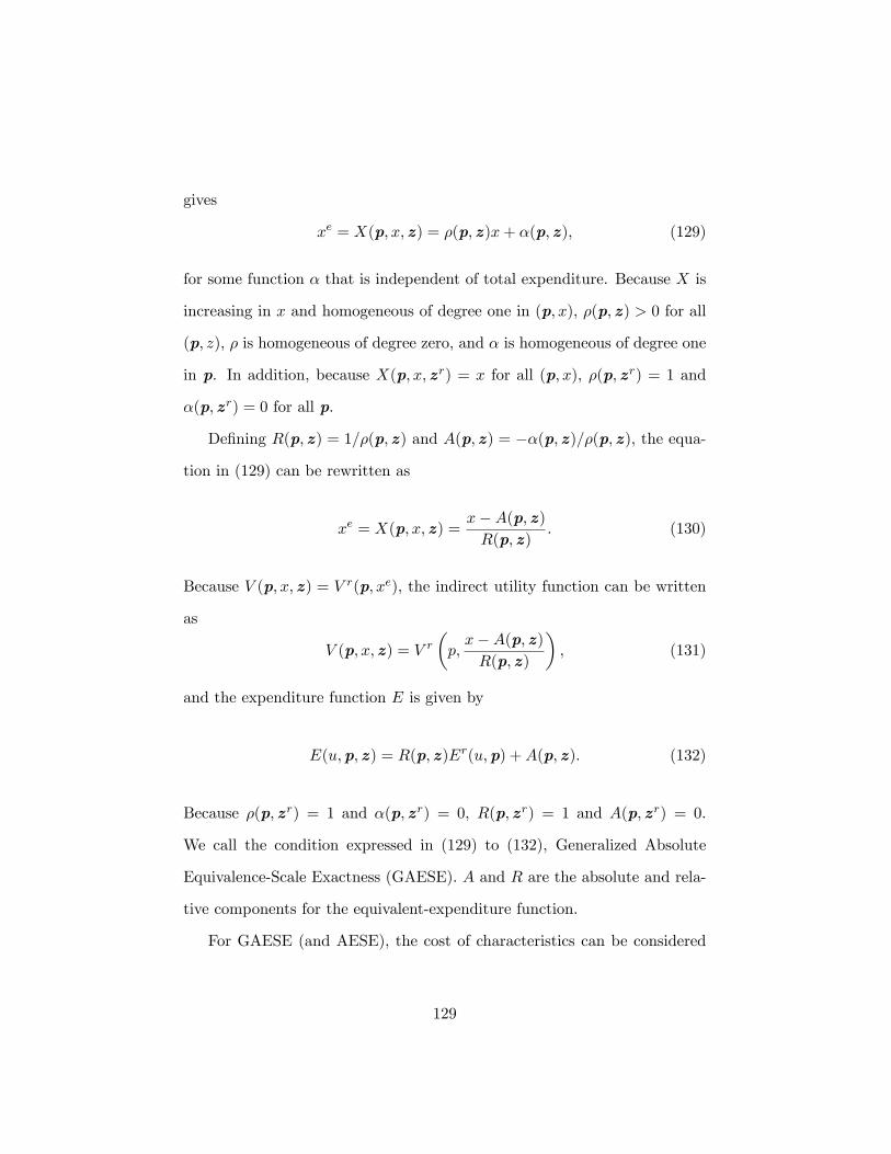
gives
xe = X(p; x;z) = �(p;z)x+ �(p;z); (129)
for some function � that is independent of total expenditure. Because X is
increasing in x and homogeneous of degree one in (p; x), �(p;z) > 0 for all
(p; z), � is homogeneous of degree zero, and � is homogeneous of degree one
in p. In addition, because X(p; x;zr) = x for all (p; x), �(p;zr) = 1 and
�(p;zr) = 0 for all p.
De�ning R(p;z) = 1=�(p;z) and A(p;z) = ��(p;z)=�(p;z), the equa-
tion in (129) can be rewritten as
xe = X(p; x;z) =x�A(p;z)R(p;z)
. (130)
Because V (p; x;z) = V r(p; xe), the indirect utility function can be written
as
V (p; x;z) = V r�p;x�A(p;z)R(p;z)
�, (131)
and the expenditure function E is given by
E(u;p;z) = R(p;z)Er(u;p) +A(p;z). (132)
Because �(p;zr) = 1 and �(p;zr) = 0, R(p;zr) = 1 and A(p;zr) = 0.
We call the condition expressed in (129) to (132), Generalized Absolute
Equivalence-Scale Exactness (GAESE). A and R are the absolute and rela-
tive components for the equivalent-expenditure function.
For GAESE (and AESE), the cost of characteristics can be considered
129
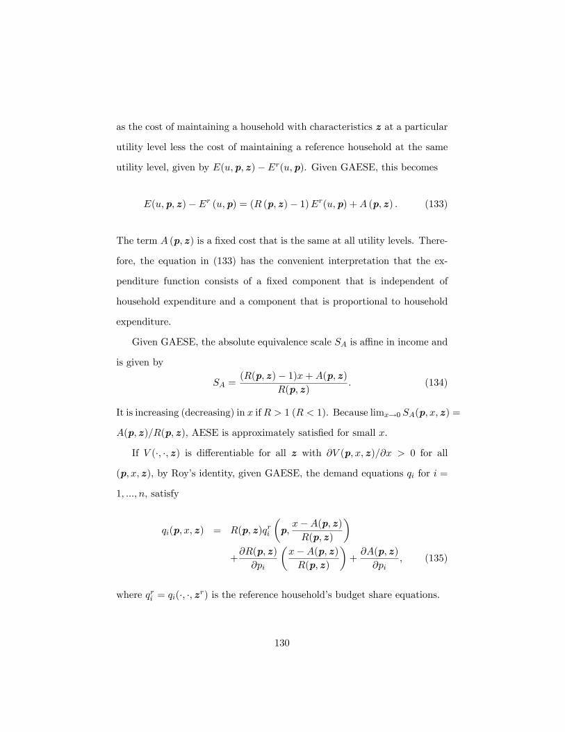
as the cost of maintaining a household with characteristics z at a particular
utility level less the cost of maintaining a reference household at the same
utility level, given by E(u;p;z)� Er(u;p). Given GAESE, this becomes
E(u;p;z)� Er (u;p) = (R (p;z)� 1)Er(u;p) +A (p;z) : (133)
The term A (p;z) is a �xed cost that is the same at all utility levels. There-
fore, the equation in (133) has the convenient interpretation that the ex-
penditure function consists of a �xed component that is independent of
household expenditure and a component that is proportional to household
expenditure.
Given GAESE, the absolute equivalence scale SA is a¢ ne in income and
is given by
SA =(R(p;z)� 1)x+A(p;z)
R(p;z). (134)
It is increasing (decreasing) in x ifR > 1 (R < 1). Because limx!0 SA(p; x;z) =
A(p;z)=R(p;z), AESE is approximately satis�ed for small x.
If V (�; �;z) is di¤erentiable for all z with @V (p; x;z)=@x > 0 for all
(p; x;z), by Roy�s identity, given GAESE, the demand equations qi for i =
1; :::; n, satisfy
qi(p; x;z) = R(p;z)qri
�p;x�A(p;z)R(p;z)
�+@R(p;z)
@pi
�x�A(p;z)R(p;z)
�+@A(p;z)
@pi, (135)
where qri = qi(�; �;zr) is the reference household�s budget share equations.
130
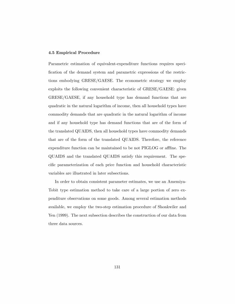
4.5 Empirical Procedure
Parametric estimation of equivalent-expenditure functions requires speci-
�cation of the demand system and parametric expressions of the restric-
tions embodying GRESE/GAESE. The econometric strategy we employ
exploits the following convenient characteristic of GRESE/GAESE: given
GRESE/GAESE, if any household type has demand functions that are
quadratic in the natural logarithm of income, then all household types have
commodity demands that are quadratic in the natural logarithm of income
and if any household type has demand functions that are of the form of
the translated QUAIDS, then all household types have commodity demands
that are of the form of the translated QUAIDS. Therefore, the reference
expenditure function can be maintained to be not PIGLOG or a¤�ne. The
QUAIDS and the translated QUAIDS satisfy this requirement. The spe-
ci�c parameterization of each price function and household characteristic
variables are illustrated in later subsections.
In order to obtain consistent parameter estimates, we use an Amemiya-
Tobit type estimation method to take care of a large portion of zero ex-
penditure observations on some goods. Among several estimation methods
available, we employ the two-step estimation procedure of Shonkwiler and
Yen (1999). The next subsection describes the construction of our data from
three data sources.
131

4.5.1 Data
Our data sets are constructed from three sources: the Japanese Panel Survey
on Consumers (JPSC) conducted and administered by the Institute for the
Research on Household Economics, and the Consumer Price Index Survey
and Family Expenditure Survey Index administered by the Statistics Bu-
reau and the Director-General for Policy Planning (Statistical Standards)
of Japan.
JPSC is panel data that tracks the personal lives of young women in
Japan over a number of years. The survey consists of a number of question-
naires, topics ranged from family members and social activities to opinions
on current issues and their personalities. The �rst survey was conducted
in 1993 when a group of 1,500 women between the ages of 24 and 34 years
was surveyed. On top of that group of women, labeled as cohort A, another
500 women between the ages of 24 and 27 were added in 1997 (cohort B).
Another 836 women with ages between 24 and 29 were added in 2003 (co-
hort C). As of 2010, the survey is still continuing. It takes place in October
of each year, and most of the information about household expenditures is
collected for expenditures made in September. It was not until 1998 that
the survey began collecting information on expenditures of subaggregated
categories of goods. The following six categories are selected in the analy-
sis: Food; Fuel, light and water charges; Furniture and household utensils;
Clothes and footwear; Transportation; Communication.57
57All expenditure categories are Food; Housing; Fuel, light and water charges; Furnitureand household utensils; Clothes and footwear; Medical care; Transportation; Communica-tion; Education; Reading and recreation; Social activity; Allowance for family members;and Miscellaneous.
132
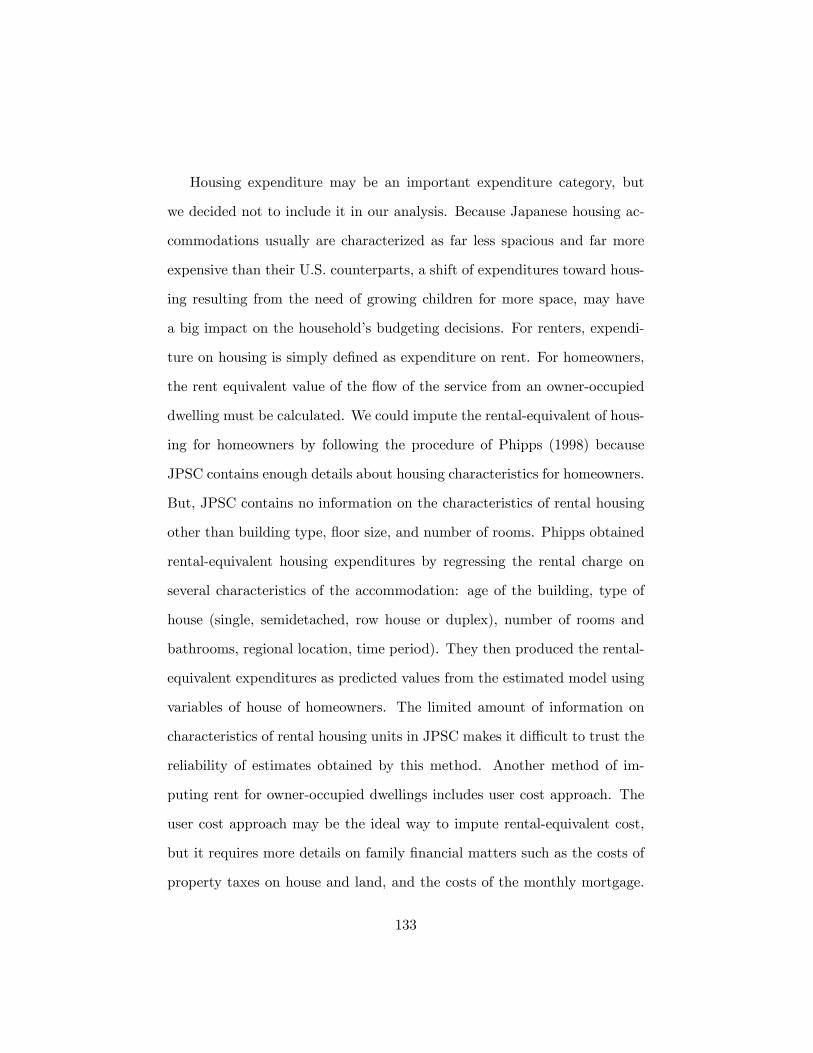
Housing expenditure may be an important expenditure category, but
we decided not to include it in our analysis. Because Japanese housing ac-
commodations usually are characterized as far less spacious and far more
expensive than their U.S. counterparts, a shift of expenditures toward hous-
ing resulting from the need of growing children for more space, may have
a big impact on the household�s budgeting decisions. For renters, expendi-
ture on housing is simply de�ned as expenditure on rent. For homeowners,
the rent equivalent value of the �ow of the service from an owner-occupied
dwelling must be calculated. We could impute the rental-equivalent of hous-
ing for homeowners by following the procedure of Phipps (1998) because
JPSC contains enough details about housing characteristics for homeowners.
But, JPSC contains no information on the characteristics of rental housing
other than building type, �oor size, and number of rooms. Phipps obtained
rental-equivalent housing expenditures by regressing the rental charge on
several characteristics of the accommodation: age of the building, type of
house (single, semidetached, row house or duplex), number of rooms and
bathrooms, regional location, time period). They then produced the rental-
equivalent expenditures as predicted values from the estimated model using
variables of house of homeowners. The limited amount of information on
characteristics of rental housing units in JPSC makes it di¢ cult to trust the
reliability of estimates obtained by this method. Another method of im-
puting rent for owner-occupied dwellings includes user cost approach. The
user cost approach may be the ideal way to impute rental-equivalent cost,
but it requires more details on family �nancial matters such as the costs of
property taxes on house and land, and the costs of the monthly mortgage.
133

We tried to make use of a variety of information on housing and real estate
for the years 1998 and 2000 complied in the Housing and Land Survey. But,
we could not extract any useful information from this source. Despite our
e¤orts to extract useful housing expenditure data for each household, the
lack of information on the characteristics of rented dwellings in JPSC hin-
ders the use of available methods to produce satisfactorily accurate values
for imputed rental-equivalence.
We de�ne each good as follows: Food includes expenditures on eating-out
and children�s school lunches as well as food in general. Utility includes ex-
penditures for electricity, gas, water, and sewer charges. Furniture includes
expenditures on durable goods such as electronic appliances and household
utensils as well as bedding. Clothing includes expenditures on clothing and
footwear. Transportation includes vehicle purchase expense, gasoline ex-
pense, and public transportation fees. Communication consists of postage
fees, and charges for telephone and Internet usage. Survey respondents are
made aware of these de�nitions.
We created variables for the number of children in the household classi-
�ed by their age group: Youji represents children under mandatory school-
age, usually less than 7 years old. Children who attend kindergarten are
included in this variable. Shou represents children who attend elementary
school, usually those between 7 and 12 years old. Chu represents children
who attend junior high school, usually those between 13 and 15 years old.
Kou represents children who attend high school, usually those between 16
and 18 years old. Since there are not enough observations of households
with high schoolers, we combine Chu and Kou to create a variable Shonen
134
for the analysis.
We estimate the child cost for typical married couples who are �nancially
independent of their parents, supportng both themselves and their children.
Based on this criteria, single women were eliminated from the sample be-
cause single-parent families headed by unmarried mothers are uncommon in
Japan. We further eliminated samples with children older than high school
age. We also eliminated those households in which all members are not
cohabitating, or with other adult members (such as grandparents).
Households that consist of several generations of family members are
able to have family members other than parents to take care of the children.
It is considered as a traditional fom of family composition. Unfortunately,
the sample selection criteria prevents us from estimating the e¤ect of hav-
ing other co-dwelling adult family members in the household. Having other
members of the family live in the household, for example, those who are
retired from market production is helpful to cover the opportunity cost as-
sociated with child-rearing. This is especially true in the case of infants
because they require constant care from parents who would be likely to be
more productive in the labor market than engaging in household production.
It may be the case that households which include the children�s grandparents
tend to have more children on that basis. This discussion is undoubtedly
related to the topic of female labor supply and fertility, another important
�eld in economics by itself. The arguments, however, regarding child cost
as one of the major reasons for the low birth-rate trend are usually centered
on the aforementioned nuclear family households which, in 2005, comprised
135

57:9 percent of the total number of Japanese household units.58 A public
policy to encourage married couples to live with their parents does not seem
appropriate as a political stance because of the extent to which it would
involve the government in private family matters. Yamaguchi (2006) recom-
mends making child-care institutions more readily available in the workplace
itself to o¤set the opportunity cost associated with child rearing.
We have prepared two sets of price data. One is the yearly average price
index, strati�ed by the level of household income for the given year, ob-
tained from the Consumer Price Index. The income level is classi�ed into
�ve quintiles. Price data for income class is presented in Table 2 along with
the value of the threshold of the quintiles. We had to construct price data
for Transportation since the original data gives public transportation and
private transportation price data separately. We aggregated the two series
as the weighted average by the expenditure share of the average Japanese
household. The data on expenditures made by average Japanese households
on a variety of goods are available in the Family Expenditure Survey. Look-
ing at Table 2, the overall de�ationary trend in prices can be seen during
the data period. It is especially noticeable in Clothing and Communication.
It probably re�ects the recent major global shift of textile manufacturing
to China for cheaper production costs and the on-going rapid development
in the Internet and associated information technology. The other dataset
is the price index for the month of September from the same source. Since
more price variation is preferred, we used the price data mentioned earlier.
We selected a number of demographic variables which is used in the �rst
58One-person households made up a 29.5 percent of the population.
136

stage estimation of the Probit model. After considering the appropriateness
of exogenous variables and the parsimoniousness of the model speci�cations
to explain the e¤ect on the occurrence of zero expenditures, we chose the fol-
lowing variables: age of the husband, the number of computer and vehicles
held in the household, total income, and dummy variables indicating urban-
ization of residence (13 big cities), credit card usage (occasional use), survey
years, wife�s employment status (employed), homeownership (public rental
housing), and education achievement levels of wife and husband. Other
than the variables selected, the household characteristics we have consid-
ered include: price index for private residential rent; price index for public
residential rent; price index for cost of repair and maintenance (from the
Consumer Price Index); typical daily time allocation of wife and husband
such as how many hours are spent on commuting etc.; units of dishwasher;
units of clothes dryers; units of air conditioners; units of TV sets; and units
of cell phones; household family �nancial management style, which has 18
di¤erent patterns.
It required some thought to construct the homeowership dummy. It is
not an unusual practice in the Japanese real estate business for a house
building itself to be owned by the resident while the land beneath it may be
rented or shared with neighbors. We have tried cases where homeownership
means that the building and land are both owned and cases where only the
building is owned. After checking the statistical signi�cance of the variables,
we found that a dummy indicating the public rental housing works better
than a dummy indicating homeownership. This indicator may be important
since living in public funded housing in Japan is a popular housing choice
137
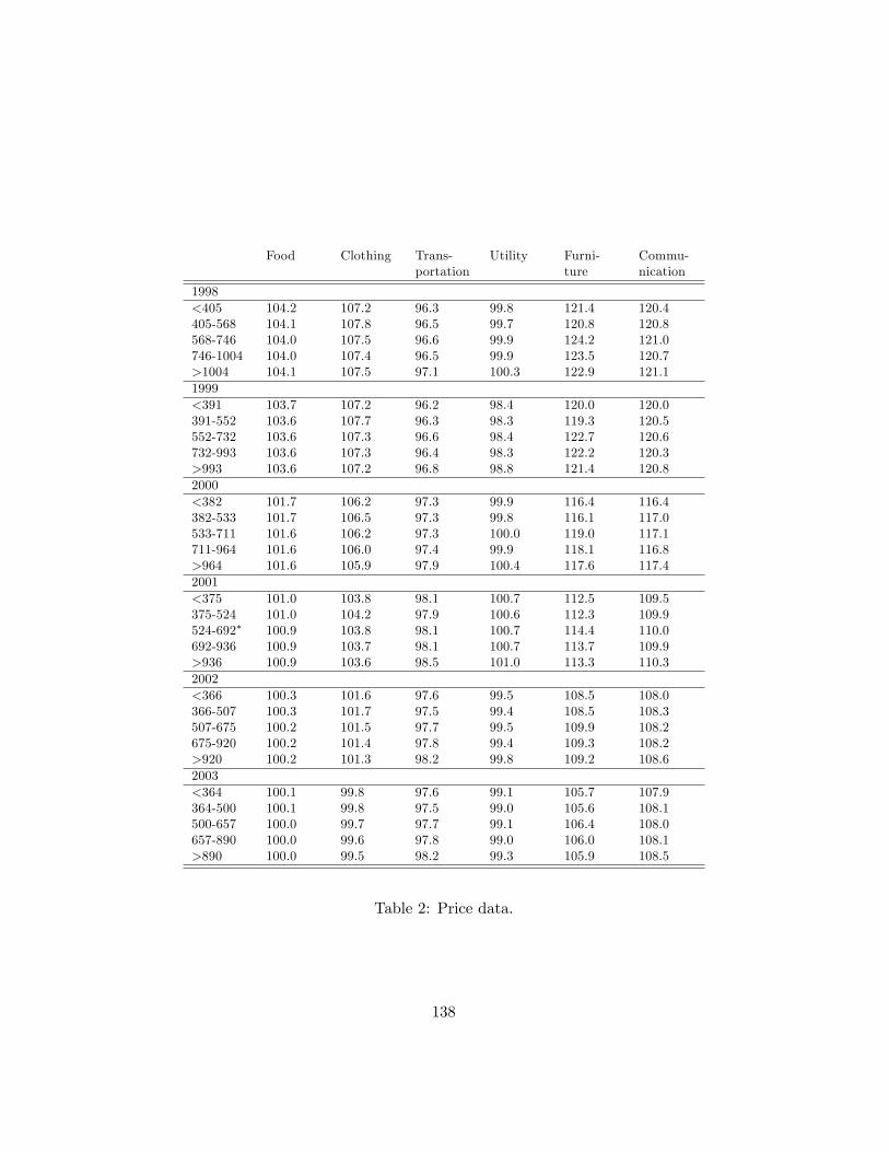
Food Clothing Trans- Utility Furni- Commu-portation ture nication
1998<405 104.2 107.2 96.3 99.8 121.4 120.4405-568 104.1 107.8 96.5 99.7 120.8 120.8568-746 104.0 107.5 96.6 99.9 124.2 121.0746-1004 104.0 107.4 96.5 99.9 123.5 120.7>1004 104.1 107.5 97.1 100.3 122.9 121.11999<391 103.7 107.2 96.2 98.4 120.0 120.0391-552 103.6 107.7 96.3 98.3 119.3 120.5552-732 103.6 107.3 96.6 98.4 122.7 120.6732-993 103.6 107.3 96.4 98.3 122.2 120.3>993 103.6 107.2 96.8 98.8 121.4 120.82000<382 101.7 106.2 97.3 99.9 116.4 116.4382-533 101.7 106.5 97.3 99.8 116.1 117.0533-711 101.6 106.2 97.3 100.0 119.0 117.1711-964 101.6 106.0 97.4 99.9 118.1 116.8>964 101.6 105.9 97.9 100.4 117.6 117.42001<375 101.0 103.8 98.1 100.7 112.5 109.5375-524 101.0 104.2 97.9 100.6 112.3 109.9524-692� 100.9 103.8 98.1 100.7 114.4 110.0692-936 100.9 103.7 98.1 100.7 113.7 109.9>936 100.9 103.6 98.5 101.0 113.3 110.32002<366 100.3 101.6 97.6 99.5 108.5 108.0366-507 100.3 101.7 97.5 99.4 108.5 108.3507-675 100.2 101.5 97.7 99.5 109.9 108.2675-920 100.2 101.4 97.8 99.4 109.3 108.2>920 100.2 101.3 98.2 99.8 109.2 108.62003<364 100.1 99.8 97.6 99.1 105.7 107.9364-500 100.1 99.8 97.5 99.0 105.6 108.1500-657 100.0 99.7 97.7 99.1 106.4 108.0657-890 100.0 99.6 97.8 99.0 106.0 108.1>890 100.0 99.5 98.2 99.3 105.9 108.5
Table 2: Price data.
138
for many young couples in suburban areas. The idea of public housing is
viewed more positively in Japanese society than in the U.S.
Yearly dummy variables do not appear to be good predictors of zero
expenditure occurrence. Nevertheless, a dummy for year 2001 was found to
be statistically signi�cant for some goods. We may interpret this as "911
terrorist attack" e¤ect. If the year 2002 dummy turned out to be signi�cant,
then we may interpreted it as the "World Cup" e¤ect since it was co-hosted
by Japan and Korea in July of 2002. The husband income and wife income
data on JPSC are marked by a number of missing records and this incident
is often encountered in microdata. We have avoided having to discard some
of the observations by assigning an income of zero for wives who appear
to be unemployed, housewives or students. The total income is the sum of
incomes from both husband and wife.
We have observed that there exit a few observations with unit budget
share. Of course, this can occur in only one good since, in that case, budget
shares of all other goods will be zero. This is perfectly legitimate since a
household can spend on goods outside of the six categories of goods which
we analyze. A household can also have zero expenditure on certain goods
even while consuming them: ones does not go naked during a time when
no clothing purchases have been made. Nevertheless, these outliers are not
favored by statistical analysis and are likely to contaminate the precision
of the parameters we would like to estimate. We found one sample of unit
value of budget share in Food, two samples in Utility, none in Furniture,
Clothing and Transportation, and one in communication. After inspecting
the histograms of the budget share data shown in Figure 7, we concluded
139
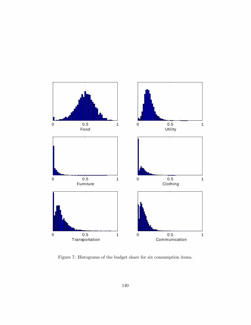
0 0.5 1Food
0 0.5 1Uti l ity
0 0.5 1Furni ture
0 0.5 1Clothing
0 0.5 1Transportation
0 0.5 1Communication
Figure 7: Histograms of the budget share for six consumption items.
140
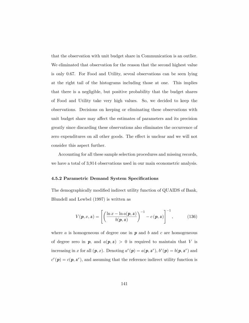
that the observation with unit budget share in Communication is an outlier.
We eliminated that observation for the reason that the second highest value
is only 0:67. For Food and Utility, seveal observations can be seen lying
at the right tail of the histograms including those at one. This implies
that there is a negligible, but positive probability that the budget shares
of Food and Utility take very high values. So, we decided to keep the
observations. Decisions on keeping or eliminating these observations with
unit budget share may a¤ect the estimates of parameters and its precision
greatly since discarding these observations also eliminates the occurrence of
zero expenditures on all other goods. The e¤ect is unclear and we will not
consider this aspect further.
Accounting for all these sample selection procedures and missing records,
we have a total of 3,914 observations used in our main econometric analysis.
4.5.2 Parametric Demand System Speci�cations
The demographically modi�ed indirect utility function of QUAIDS of Bank,
Blundell and Lewbel (1997) is written as
V (p; x;z) =
"�lnx� ln a(p;z)
b(p;z)
��1� c (p;z)
#�1; (136)
where a is homogeneous of degree one in p and b and c are homogeneous
of degree zero in p, and a(p;z) > 0 is required to maintain that V is
increasing in x for all (p; x). Denoting ar(p) = a(p;zr), br(p) = b(p;zr) and
cr(p) = c(p;zr), and assuming that the reference indirect utility function is
141
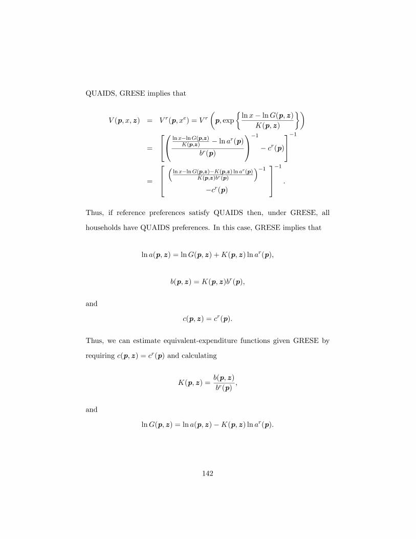
QUAIDS, GRESE implies that
V (p; x;z) = V r(p; xe) = V r�p; exp
�lnx� lnG(p;z)
K(p;z)
��
=
240@ lnx�lnG(p;z)K(p;z) � ln ar(p)
br(p)
1A�1 � cr(p)35�1
=
264�lnx�lnG(p;z)�K(p;z) ln ar(p)
K(p;z)br(p)
��1�cr(p)
375�1
.
Thus, if reference preferences satisfy QUAIDS then, under GRESE, all
households have QUAIDS preferences. In this case, GRESE implies that
ln a(p;z) = lnG(p;z) +K(p;z) ln ar(p);
b(p;z) = K(p;z)br(p),
and
c(p;z) = cr(p).
Thus, we can estimate equivalent-expenditure functions given GRESE by
requiring c(p;z) = cr(p) and calculating
K(p;z) =b(p;z)
br(p),
and
lnG(p;z) = ln a(p;z)�K(p;z) ln ar(p).
142
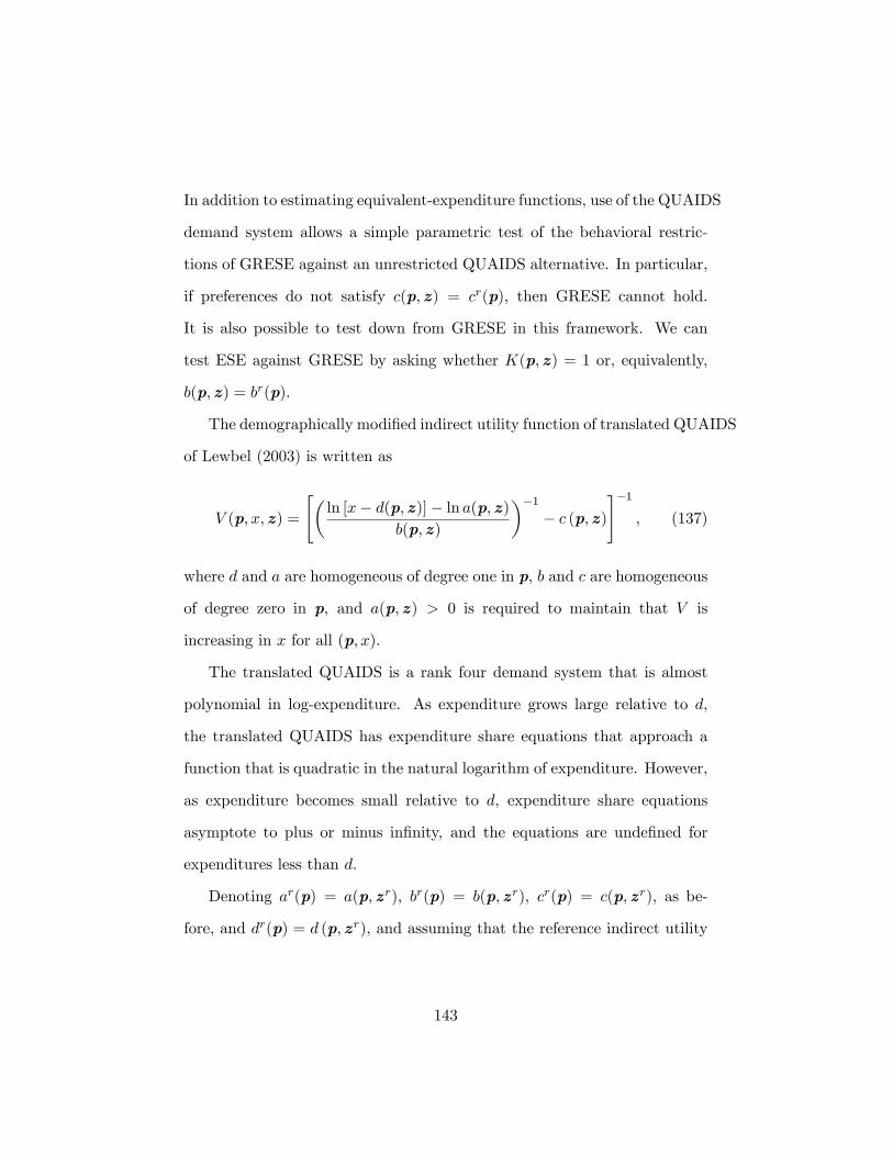
In addition to estimating equivalent-expenditure functions, use of the QUAIDS
demand system allows a simple parametric test of the behavioral restric-
tions of GRESE against an unrestricted QUAIDS alternative. In particular,
if preferences do not satisfy c(p;z) = cr(p), then GRESE cannot hold.
It is also possible to test down from GRESE in this framework. We can
test ESE against GRESE by asking whether K(p;z) = 1 or, equivalently,
b(p;z) = br(p).
The demographically modi�ed indirect utility function of translated QUAIDS
of Lewbel (2003) is written as
V (p; x;z) =
"�ln [x� d(p;z)]� ln a(p;z)
b(p;z)
��1� c (p;z)
#�1; (137)
where d and a are homogeneous of degree one in p, b and c are homogeneous
of degree zero in p, and a(p;z) > 0 is required to maintain that V is
increasing in x for all (p; x).
The translated QUAIDS is a rank four demand system that is almost
polynomial in log-expenditure. As expenditure grows large relative to d,
the translated QUAIDS has expenditure share equations that approach a
function that is quadratic in the natural logarithm of expenditure. However,
as expenditure becomes small relative to d, expenditure share equations
asymptote to plus or minus in�nity, and the equations are unde�ned for
expenditures less than d.
Denoting ar(p) = a(p;zr), br(p) = b(p;zr), cr(p) = c(p;zr), as be-
fore, and dr(p) = d (p;zr), and assuming that the reference indirect utility
143
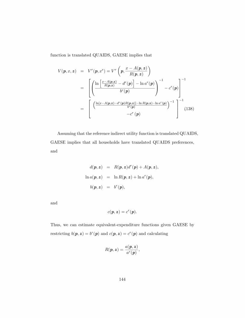
function is translated QUAIDS, GAESE implies that
V (p; x;z) = V r(p; xe) = V r�p;x�A(p;z)R(p;z)
�
=
2640@ ln
hx�A(p;z)R(p;z) � dr(p)
i� ln ar(p)
br(p)
1A�1 � cr(p)375�1
=
264�ln[x�A(p;z)�dr(p)R(p;z)]�lnR(p;z)�ln ar(p)
br(p)
��1�cr (p)
375�1
.(138)
Assuming that the reference indirect utility function is translated QUAIDS,
GAESE implies that all households have translated QUAIDS preferences,
and
d(p;z) = R(p;z)dr(p) +A(p;z);
ln a(p;z) = lnR(p;z) + ln ar(p);
b(p;z) = br(p);
and
c(p;z) = cr(p).
Thus, we can estimate equivalent-expenditure functions given GAESE by
restricting b(p;z) = br(p) and c(p;z) = cr(p) and calculating
R(p;z) =a(p;z)
ar(p);
144
and
A(p;z) = d(p;z)�R(p;z)dr(p). (139)
With these speci�cations for d, a, b, and c, A can be either positive or
negative, but R is positive.
In addition to estimating equivalent-expenditure functions under GAESE,
using the translated QUAIDS allows a simple parametric test of GAESE
against an unrestricted translated QUAIDS alternative. In particular, if
preferences do not satisfy c(p;z) = cr(p) and b(p;z) = br(p), then GAESE
cannot hold. It is also possible to test down from GAESE in this framework.
We can test AESE against GAESE by asking whether R(p;z) = 1 or, equiv-
alently, a(p;z) = ar(p). Furthermore, we can test ESE against GAESE by
asking whether A(p;z) = 0, which is true only if d(p;z) = 0.
To estimate QUAIDS demand system, we specify the functions, a, b, and
c as
ln a(p;z) = a0(z) +nXk=1
ak(z) ln pk +1
2
nXk=1
nXk=1
akl ln pk ln pl; (140)
wherePnk=1 ak(z) = 1,
Pnl=1 akl(z) = 0 for all k, and akl = alk for all k and
l,
b(p;z) =1
1� b0(z)exp
(nXk=1
bk(z) ln pk
), (141)
wherePnk=1 bk(z) = 0, and
c(p;z) =
nXk=1
ck(z) ln pk, (142)
145
wherePnk=1 ck(z) = 0.
The functions ak, bk, and ck depend on z, and we assume the linear
speci�cation such that:
ak(z) = ark + aYoujik Youji+ aShouk Shou+ aShonenk Shonen; (143)
bk(z) = brk + bYoujik Youji+ bShouk Shou+ bShonenk Shonen, (144)
for k = 0; :::; n, and
ck(z) = crk + cYoujik Youji+ cShouk Shou+ cShonenk Shonen, (145)
for k = 1; :::; n. Youji is the natural logarithm of the number of children
younger than 7 plus one, Shou indicates the natural logarithm of the number
of children between the ages of 7 and 12 plus one, and Shoen is the natural
logarithm of the number of children between the ages of 13 and 18 plus
one.59 Other household characteristics can be incorporated into the equa-
tions (143), (144) , and (145) such as geographical location, housing tenure,
and education level of husband and wife, etc. Since those demographic char-
acteristics are used for the Probit estimation of sample selection equations,
we do not include them in the demand system.
Two parameters are set rather than estimated. We set ar0 so that ln a(p;zr)
is equal to the average expenditure of the reference household (a household
without any children) in 2001 (the middle year of data).60 We set br0 = 0
59 Including the number of children in di¤erent age bands may induces discontinuitiesthat are certainly spurious. Browning (1992) suggests using as a variable the average ageof the children in the household.60The average total expenditure for the 2001 panel is 1:303 (in unit of 100,000 yen).
146
for identi�cation purpose.
The restrictions in (140) to (142) are carried over to the restrictions
imposed on (143) to (145) such that:
nXk=1
ark = 1, (146)
nXk=1
aYoujik =nXk=1
aShouk =nXk=1
aShonenk = 0, (147)
nXk=1
brk =nXk=1
bYoujik =nXk=1
bShouk =nXk=1
bShonenk = 0, (148)
nXk=1
crk =nXk=1
cYoujik =nXk=1
cShouk =nXk=1
cShonenk = 0: (149)
Applying the logarithm form of Roy�s identity produces the log-quadratic
expenditure budget share equations
wi(p; x;z) =@ ln a(p;z)
@ ln pi+@ ln b(p;z)
@ ln pi(lnx� ln a(p;z))
+@q(p;z)
@ ln pi
(lnx� ln a(p;z))2b(p;z)
, (150)
for i = 1; :::; n. Substituting equations (140) - (142) into (150), we get
wi(p; x;z) =
ai(z) +
nXk=1
arik ln pk
!+ bi(z)(lnx� ln a(p;z))
+ci(z)(1� b0(z))(lnx� ln a(p;z))2
exp
(nXk=1
bk(z) ln pk
) , (151)
for i = 1; :::; n.
147
GRESE requires ck(z) = crk for all k = 1; :::; n. Thus, given QUAIDS
demands, GRESE restricts preferences in such a way that the coe¢ cients on
(lnx)2 are proportional across household types. To test up from GRESE,
we estimate a model in which GRESE is not maintained so that these pro-
portionality restrictions are relaxed. In that case, the share equations are
homogeneous in (b0(z); c1(z); :::; cn(z)), so that these functions are not sep-
arately identi�able. Doubling b0 (z) halves all ck (z)�s. To identify ck(z) in
the unrestricted QUAIDS, we impose the restriction b0(z) = 0. However,
under GRESE, this restriction is not necessary because ck(z) = crk, and we
use the weaker restriction that b0(zr) = br0 = 0.
GRESE can be also tested down. One can test whether or not K(p;z) =
1 which gives ESE by testing the additional restriction that b0(z) = br0 = 0
in a GRESE-restricted model.
Given GRESE, equivalent-expenditure functions are uniquely identi�-
able if and only if GRESE is maintained a priori and the reference expendi-
ture function is not PIGLOG. The QUAIDS model is PIGLOG if and only
if c(p;z) = 0. Thus, we may test identi�cation restrictions of GRESE of
testing crk = 0 for all k, in a GRESE-restricted model.
With the GRESE-restricted QUAIDS model, the GRESE functions K
and G take on relatively simple forms in terms of the parameters if evaluated
at an n-vector of equal prices p� = 1, with
K(p�;z) =1
1� b0(z)
148
and
lnG (p�;z) = a0(z)�ar0
1� b0(z).
Substituting these expressions into equation (120) and manipulating, we get
a simple expression for the log-equivalence scale evaluated at a vector of unit
prices:
lnSR(p�; x;z) = b0(z) (lnx� a0(z)) + (a0(z)� ar0). (152)
The �rst term is zero if lnx = a0(z), which by construction is true for house-
holds whose equivalent expenditure is equal to the average expenditure of
the reference households in the base year 2001. Thus, lnS (p�; a(p�;z);z) =
a0(z)�ar0. If ESE is true, then b0(z) = 0, so that the equivalence scale takes
this form at all levels of expenditure.
To estimate the translated QUAIDS demand systems, we specify the
functions d, a, b, and c as
d(p;z) =nXk=1
dk(z)pk;
a(p;z) = a0(z) +
nXk=1
ak(z) ln pk +1
2
nXk=1
nXl=1
akl ln pk ln pl, (153)
wherePnk=1 ak(z) = 1,
Pnl=1 akl(z) = 0 for all k and akl = alk for all k and
l,
ln b(p;z) =nXk=1
bk(z) ln pk, (154)
149
wherePnk=1 bk(z) = 0, and
c(p;z) =nXk=1
ck(z) ln pk, (155)
wherePnk=1 ck(z) = 0.
It is convenient to denote
d0(z) =nXk=1
dk(z). (156)
The functions dk, ak, bk, and ck depend on z, and we assume that
dk(z) = drk + aYoujik Youji+ aShouk Shou+ aShonenk Shonen, (157)
ak(z) = ark + aYoujik Youji+ aShouk Shou+ aShonenk Shonen; (158)
bk(z) = brk + bYoujik Youji+ bShouk Shou+ bShonenk Shonen, (159)
ck(z) = crk + cYoujik Youji+ cShouk Shou+ cShonenk Shonen, (160)
for k = 1; :::; n. Youji is the natural logarithm of the number of children
younger than 6 plus one, Shou indicates the natural logarithm of the num-
ber of children between the ages of 7 and 12 plus one, and Shonen is the
natural logarithm of the number of children between the ages of 13 and
18 plus one. Other household characteristics can be incorporated into the
equations in (157), (158), (159), and (160) such as geographical location,
housing tenure, and education level of husband and wife, etc. Since those
demographic characteristics are used �rst in the Probit estimation for the
two-step estimation procedure, we do not include them in the demand sys-
150
tem.
The restrictions in (153) to (155) are carried over to the restrictions
imposed on (157) to (160) such that:
nXk=1
ark = 1, (161)
nXk=1
aYoujik =nXk=1
aShouk =nXk=1
aShonenk = 0, (162)
nXk=1
brk =nXk=1
bYoujik =nXk=1
bShouk =nXk=1
bShonenk = 0, (163)
nXk=1
crk =nXk=1
cYoujik =nXk=1
cShouk =nXk=1
cShonenk = 0. (164)
There are no restrictions on dk�s.
We note that, with the translated QUAIDS speci�cation, the GAESE
functions A and R take on relatively simple forms in terms of the parameters
if evaluated at an n-vector of unit prices p� = 1 with
R(p�;z) = exp(a0(z)� a0 (zr))
and
A(p�;z) = (d0(z)� exp(a0(z)� a0(zr))d0(zr)).
The GAESE in (134) becomes
SA =(exp(a0(z)� ar0)� 1)x+ (d0(z)� exp(a0(z)� ar0)dr0)
exp(a0(z)� ar0). (165)
Applying Roy�s theorem in its logarithmic form to (138) generates the
151
expenditure share equations
wi =pidi(z)
x+
�1� d(p;z)
x
��0B@ ai(z) +
Pnk=1 aik ln pk + bi(z)
�ln x�d(p;z)a(p;z)
�+ ci(z)b(p;z)
�ln x�d(p;z)a(p;z)
�21CA ; (166)
for i = 1; ::; n. Equation (166) does not necessarily satisfy GAESE, which
requires that bk(z) = brk and ck(z) = crk. The translated QUAIDS demand
system corresponds to an a¢ ne expenditure function if and only if b(p;z)
and c(p;z) are both 0, and corresponds to a log-a¢ ne expenditure function
if and only if d(p;z) and c (p;z) are both 0. Because equivalent-expenditure
functions given GAESE are uniquely identi�able if the expenditure function
is neither a¢ ne nor log-a¢ ne, identi�cation is possible given GAESE if c is
nonzero or if both d and b are nonzero.
4.5.3 Estimation
The usual procedure to estimate the demand systems is to append an error
term " to the right-hand side of the share equations and then estimate the
model by ML or iterative SUR, assuming the joint normal distribution of the
errors term. As mentioned, this usual estimation procedure is not applicable
for our data due to the presence of a large pile of zero expenditures in some
of the goods.
In microeconomics data on consumer expenditure, it is frequently the
case that some units do not purchase some of the commodities, alcohol and
152
tobacco being the standard examples.61 Microeconomics theory predicts it
as the case of a corner solution of the optimization problem as opposed to the
interior solution. When the relative price of goods is too high, the consumer
may choose not to consumer the good at all as the optimal consumption
allocation. Although the zero expenditure on some goods is entirely consis-
tent with the theory of consumer behavior, the estimation faces a serious
problem in dealing with it. In the presence of a mass of zero expenditure
observations, a joint normal distribution of error structure does not allow
for a signi�cant proportion of realization at zero expenditure.62 Standard
estimation methods for this model such as SUR or maximum likelihood es-
timator do not take special account of zero expenditures, and consequently
yield inconsistent estimates of the parameters. Even if observations contain-
ing zero expenditures on one or more goods were eliminated for purposes
of estimation, these standard estimators would be biased and inconsistent.
Moreover, excluding these observations might signi�cantly reduce the sam-
ple size. Regardless of whether or not the complete sample is used, the bias
and inconsistency occur because the random disturbances have expectations
which are not zero and which depend upon the exogenous variables. The
easiest way to deal with zero expenditure is to form a broader aggregate
commodity category. Hoderlein (2008) grouped his housing goods category
61Fry and Pashardes (1994) studied the tobacco expenditures, Su and Yen (2000) studiedthe demands for alcohol and tobacco products with a number of zero-expenditure samplesin their data, and Unayama (2006) examined the rank of demand function for alcohol.62Woodland (1979) proposed that the error terms be modelled as Dirichlet or log-normal
distribution for the purpose of restricting the deterministic part and disturbance part ofbudget share to the closed unit interval [0; 1]. His method does not solve zero expenditureissue since Dirichlet (and log-normal) distribution cannot model a sharp increase of theprobability of expenditure at zero.
153
as a combination of rent or mortgage payment, furniture, and household
goods and services which reduces the occurrence of zero expenditures on
each of these subcategories.
Assuming that the zero expenditure occurs as a result of the corner solu-
tion, the econometric methods based on the Kuhn-Tucker conditions (Wales
and Woodland, 1983) and on the virtual prices, which is dual to the Kuhn-
Tucker conditions (Lee and Pitt, 1986, 1987), have been developed.63 How-
ever, because any of the methods usually requires the evaluation of multiple
integration to calculate the value of likelihood function in each iteration, the
application is limited to very restrictive forms of the demand model. The
simulation and Bayesian methods have been proposed to circumvent the
curse of dimensionality (Kao, Lee and Pitt, 2001, Millimet and Tchernis,
2008, Pitt and Millimet, 1999).64
Households may appear to have bought none of some particular goods
not because they are too expensive, but because the enumeriation period
was too short. Storable or durable goods such as canned foods and clothing
are frequently not purchased during the survey period even if they are used
during that time. Zero purchases of clothing during the particular weeks or
month of a survey period does not mean that people go naked during that
period.65 This problem had been noticed for a while, and Deaton and Irish
(1982) �nally attempted to estimate a econometric model of the household
63An earlier attempt to take a possible corner solution into account in demand analysisincludes Barnett (1979).64The estimation of demand systems by Bayesian methods are studied by Barnett,
Geweke and Wolfe (1991a, 1991b), Terrell (1996).65JPSC collects expenditures made during the entire month of September. We do not
know whether a one-month enumeration period is long enough or is too short.
154
demand behavior with zero expenditure samples which are assumed to be
generated by the infrequent purchase. Deaton and Irish (1984) present a p-
tobit model that extends the tobit speci�cation to model zero expenditures.
Recorded data for expenditure on commodities are 1=p times consumption
during the survey period, where p denotes the ratio of the survey period to
the purchase period. This is applicable when goods are consumed during
the survey period; however, expenditures are only observed with a proba-
bility p because of infrequent purchasing (Deaton and Irish, 1984). Kay,
Keen and Morris (1984) extend the model proposed by Deaton and Irish
(1984) by providing a stochastic relationship between expenditure and con-
sumption in a sophisticated manner. Keen (1986) estimates a system of
linear Engel functions that satisfy the adding-up condition and derives a
consistent estimator based on the instrumental variables method. While
the purchasing probabilities are constant parameters in Deaton and Irish
(1984), Kay, Keen and Morris (1984) and Keen (1986), Blundell and Meghir
(1987) propose a model with probit-type purchasing probabilities. Gri¢ ths
and Valenzuela (1998), Hasegawa, Ueda and Mori (2008) estimate a system
of linear Engel functions and equivalence scales using a Bayesian method,
and Pudney (1989, 1990) reviews several theoretical aspects associated with
zero expenditures.
Another alternative approache is the Amemiya-Tobin approach which
explicitly takes into account the censored nature of the negative quantities
demanded. It has been applied where estimation is via full information
maximum likelihood (Wales and Woodland, 1983; Yen and Lin, 2004), quasi-
maximum likelihood (Yen, Lin and Smallwood, 2003), or various two-step
155
estimators (Heien and Wessell, 1993; Perali and Chavas, 1998; Shonkwiler
and Yen, 1999; Meyerhoefer, Ranney and Sahn, 2003).
In this empirical section, we employ a variant of the bivariate sample
selection model of Heckman (1974). The model can be viewed as a sample
selection generalization of Amemiya�s Tobit system. The estimation is done
in two steps instead of doing a full maximum likelihood estimation at all
once.66 The two-step procedure guarantees the consistency of the estimates
as long as parameters of each step are consistent, but it results in the loss of
e¢ cient estimation. The next section illustrates the two-step estimation pro-
cedure in Shonkwiler and Yen (1999) which has corrected the inconsistency
issue found in Heien and Wessell (1993).
The usual way to deal with the endogeniety likely to exist in demand
systems is to use income or some functions of income as instruments and
estimate the system by GMM. As long as we use this two-step estimation
procedure, we cannot use GMM in the second step. We may literally replace
the total expenditure with the projection of the total expenditure, but the
theoretical validity of doing this is questionable.
4.5.4 The Two-Step Estimation Procedure
The idea of this procedure is that one equation describes the household�s
decision to participate in the market in the similar way to the original frame-
work for female labor supply study of Heckman (1974), and a set of equations
describes the consumption behavior provided that a decision has been made
to participate in the market. A formal structure is considered in which
66The full ML estimation procedure is provided in Yen and Lin (2004)
156
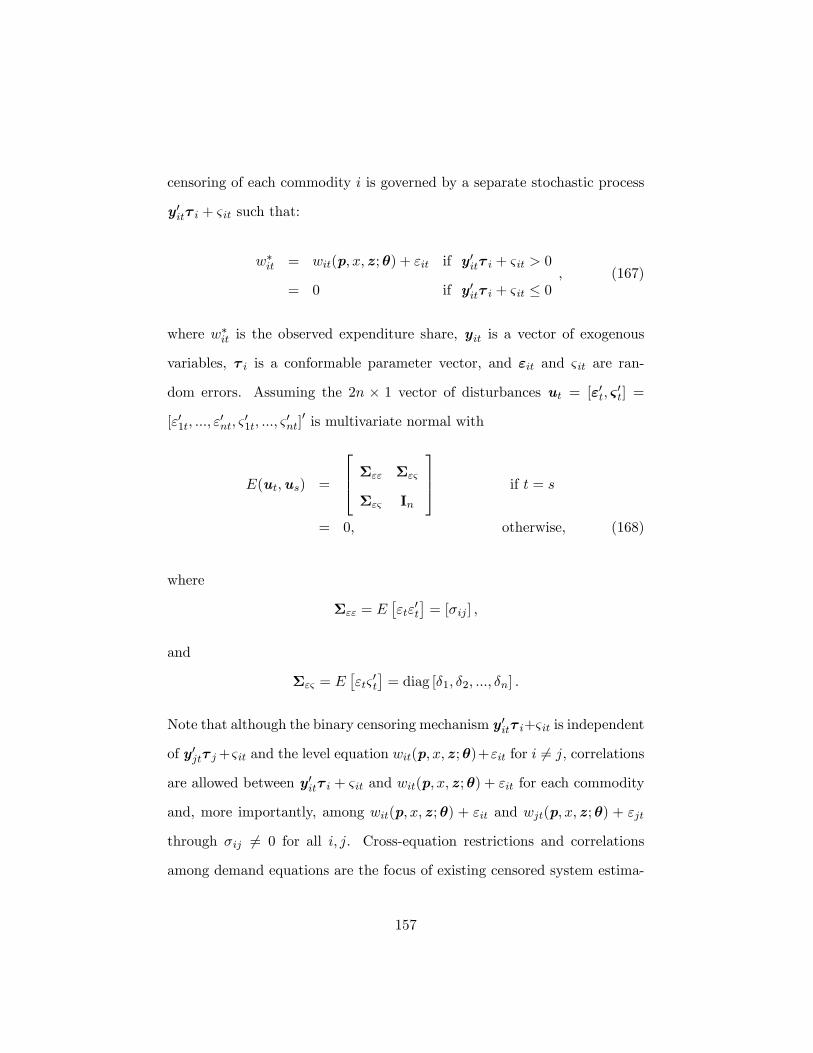
censoring of each commodity i is governed by a separate stochastic process
y0it� i + & it such that:
w�it = wit(p; x;z;�) + "it if y0it� i + & it > 0
= 0 if y0it� i + & it � 0; (167)
where w�it is the observed expenditure share, yit is a vector of exogenous
variables, � i is a conformable parameter vector, and "it and & it are ran-
dom errors. Assuming the 2n � 1 vector of disturbances ut = ["0t; &0t] =
["01t; :::; "0nt; &
01t; :::; &
0nt]0 is multivariate normal with
E(ut;us) =
264 �"" �"&
�"& In
375 if t = s
= 0; otherwise, (168)
where
�"" = E�"t"
0t
�= [�ij ] ;
and
�"& = E�"t&
0t
�= diag [�1; �2; :::; �n] .
Note that although the binary censoring mechanism y0it� i+& it is independent
of y0jt� j+& it and the level equation wit(p; x;z;�)+"it for i 6= j, correlations
are allowed between y0it� i + & it and wit(p; x;z;�) + "it for each commodity
and, more importantly, among wit(p; x;z;�) + "it and wjt(p; x;z;�) + "jt
through �ij 6= 0 for all i; j. Cross-equation restrictions and correlations
among demand equations are the focus of existing censored system estima-
157
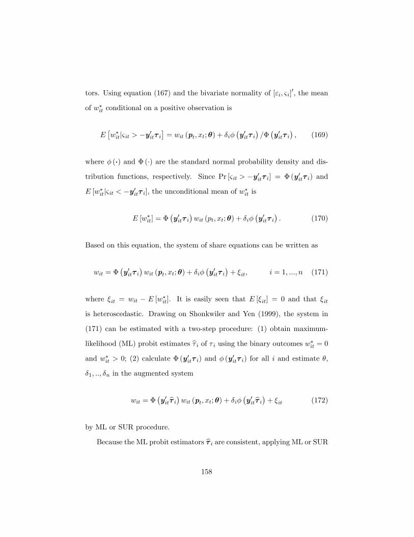
tors. Using equation (167) and the bivariate normality of ["i; & i]0, the mean
of w�it conditional on a positive observation is
E�w�itj& it > �y0it� i
�= wit (pt; xt;�) + �i�
�y0it� i
�=��y0it� i
�; (169)
where � (�) and � (�) are the standard normal probability density and dis-
tribution functions, respectively. Since Pr [& it > �y0it� i] = � (y0it� i) and
E [w�itj& it < �y0it� i], the unconditional mean of w�it is
E [w�it] = ��y0it� i
�wit (pt; xt;�) + �i�
�y0it� i
�: (170)
Based on this equation, the system of share equations can be written as
wit = ��y0it� i
�wit (pt; xt;�) + �i�
�y0it� i
�+ �it, i = 1; :::; n (171)
where �it = wit � E [w�it]. It is easily seen that E [�it] = 0 and that �it
is heteroscedastic. Drawing on Shonkwiler and Yen (1999), the system in
(171) can be estimated with a two-step procedure: (1) obtain maximum-
likelihood (ML) probit estimates b� i of � i using the binary outcomes w�it = 0and w�it > 0; (2) calculate � (y0it� i) and � (y
0it� i) for all i and estimate �,
�1; ::; �n in the augmented system
wit = ��y0itb� i�wit (pt; xt;�) + �i� �y0itb� i�+ �it (172)
by ML or SUR procedure.
Because the ML probit estimators b� i are consistent, applying ML or SUR158
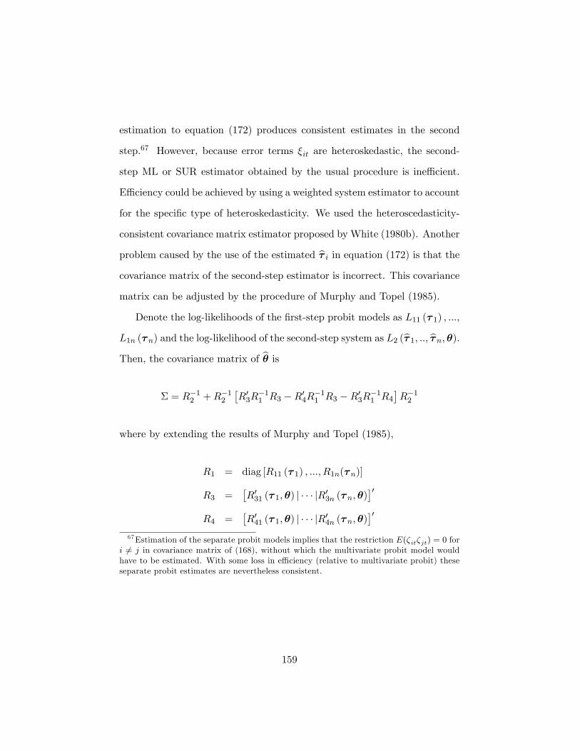
estimation to equation (172) produces consistent estimates in the second
step.67 However, because error terms �it are heteroskedastic, the second-
step ML or SUR estimator obtained by the usual procedure is ine¢ cient.
E¢ ciency could be achieved by using a weighted system estimator to account
for the speci�c type of heteroskedasticity. We used the heteroscedasticity-
consistent covariance matrix estimator proposed by White (1980b). Another
problem caused by the use of the estimated b� i in equation (172) is that thecovariance matrix of the second-step estimator is incorrect. This covariance
matrix can be adjusted by the procedure of Murphy and Topel (1985).
Denote the log-likelihoods of the �rst-step probit models as L11 (� 1) ; :::;
L1n (�n) and the log-likelihood of the second-step system as L2 (b� 1; ::; b�n;�).Then, the covariance matrix of b� is
� = R�12 +R�12�R03R
�11 R3 �R04R�11 R3 �R03R�11 R4
�R�12
where by extending the results of Murphy and Topel (1985),
R1 = diag [R11 (� 1) ; :::; R1n(�n)]
R3 =�R031 (� 1;�) j � � � jR03n (�n;�)
�0R4 =
�R041 (� 1;�) j � � � jR04n (�n;�)
�067Estimation of the separate probit models implies that the restriction E(�it�jt) = 0 for
i 6= j in covariance matrix of (168), without which the multivariate probit model wouldhave to be estimated. With some loss in e¢ ciency (relative to multivariate probit) theseseparate probit estimates are nevertheless consistent.
159
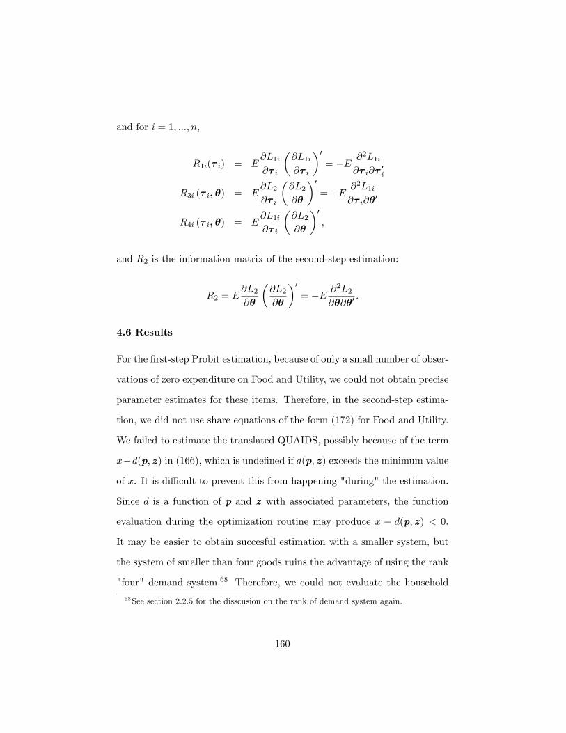
and for i = 1; :::; n,
R1i(� i) = E@L1i@� i
�@L1i@� i
�0= �E @2L1i
@� i@� 0i
R3i (� i; �) = E@L2@� i
�@L2@�
�0= �E @2L1i
@� i@�0
R4i (� i; �) = E@L1i@� i
�@L2@�
�0,
and R2 is the information matrix of the second-step estimation:
R2 = E@L2@�
�@L2@�
�0= �E @2L2
@�@�0:
4.6 Results
For the �rst-step Probit estimation, because of only a small number of obser-
vations of zero expenditure on Food and Utility, we could not obtain precise
parameter estimates for these items. Therefore, in the second-step estima-
tion, we did not use share equations of the form (172) for Food and Utility.
We failed to estimate the translated QUAIDS, possibly because of the term
x�d(p;z) in (166), which is unde�ned if d(p;z) exceeds the minimum value
of x. It is di¢ cult to prevent this from happening "during" the estimation.
Since d is a function of p and z with associated parameters, the function
evaluation during the optimization routine may produce x � d(p;z) < 0.
It may be easier to obtain succesful estimation with a smaller system, but
the system of smaller than four goods ruins the advantage of using the rank
"four" demand system.68 Therefore, we could not evaluate the household
68See section 2.2.5 for the disscusion on the rank of demand system again.
160
preferences for GAESE and the possibility that there exists a �xed cost as-
sociated only with di¤erent number of children regardless the level of utility
or income.69
We also found the singularity of covariance matrix when the full set of
n equations is estimated in GRESE case. The two-step procedure allows
for the estimation of the full system unlike usual demand system estimation
procedure. Since the augmented system does not require the adding-up to
unity, the covariance matrix is not singular by construction. We follow the
plausible and simple approach, suggested by Pudney (1989), of treating the
nth good as a residual category with no speci�c demand of its own and es-
timated the rest of n� 1 equations; our nth item is transportation. Table 3
presents some parameter estimates associated with the calculation of equiv-
alence scale, and the log-likelihood values with their number of parameters
to calculate likelihood ratio test statistics. All speci�cation tests are based
on the likelihood ratio test.70
We look at the model statistics for four models: (1) unrestricted QUAIDS;
(2) GRESE-restricted QUAIDS; (3) ESE-restricted QUAIDS; and (4) un-
restricted AIDS as shown. For the case (4), the equivalence scale is not
identi�ed, but we can test it against the alternative that the model contains
the quadratic term as QUAIDS. If AIDS model is accepted, then the equiv-
alence scale obtained is not unique either under GRESE or ESE, and it is
di¢ cult to draw any conclusion from the resulting estimates of equivalence
scales. Given the maintained assumption of GRESE restricted QUAIDS,
69The GAESE speci�cation of household preferences can be implemented with QES.We will discuss this in the conclusion section of this dissertation.70The likelihood test is known to have a tendency to over-reject the hypothesis.
161
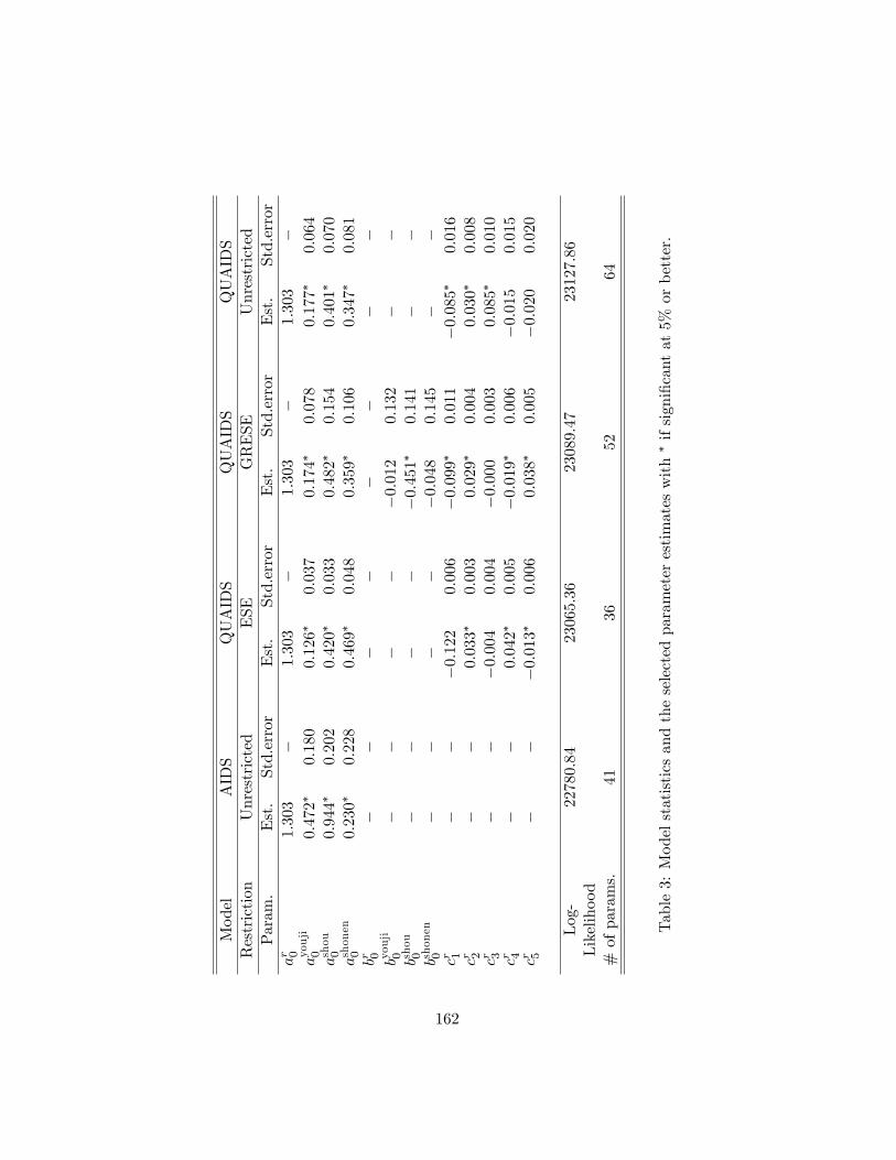
Model
AIDS
QUAIDS
QUAIDS
QUAIDS
Restriction
Unrestricted
ESE
GRESE
Unrestricted
Param.
Est.
Std.error
Est.
Std.error
Est.
Std.error
Est.
Std.error
ar 0
1:303
�1:303
�1:303
�1:303
�ayouji
00:472�
0:180
0:126�
0:037
0:174�
0:078
0:177�
0:064
ashou
00:944�
0:202
0:420�
0:033
0:482�
0:154
0:401�
0:070
ashonen
00:230�
0:228
0:469�
0:048
0:359�
0:106
0:347�
0:081
br 0�
��
��
��
�byouji
0�
��
��0:012
0:132
��
bshou
0�
��
��0:451�
0:141
��
bshonen
0�
��
��0:048
0:145
��
cr 1�
��0:122
0:006
�0:099�
0:011
�0:085�
0:016
cr 2�
�0:033�
0:003
0:029�
0:004
0:030�
0:008
cr 3�
��0:004
0:004
�0:000
0:003
0:085�
0:010
cr 4�
�0:042�
0:005
�0:019�
0:006
�0:015
0:015
cr 5�
��0:013�
0:006
0:038�
0:005
�0:020
0:020
Log-
22780:84
23065:36
23089:47
23127:86
Likelihood
#ofparams.
4136
52
64
Table3:Modelstatisticsandtheselectedparameterestimateswith�ifsigni�cantat5%orbetter.
162

ESE instead requires that b(p;z) = b(p). The likelihood ratio test statistics
for this hypothesis is 48:22 and is distributed as a �216 which has a one-
sided one percent critical value of 32. Therefore, the test prefers GRESE
speci�cation of QUAIDS model. Given an unrestricted QUAIDS model,
GRESE requires that c(p;z) = c (p)and that b(p;z) = b(p). The likelihood
ratio statistics is 76:78 and is distributed as a �212 which has a one-sided
one percent critical value of 26. Thus, the observable restrictions imposed
by GRESE on the QUAIDS model are rejected. Demographic e¤ects may
a¤ect the household demand behaviors in a more complicated way than
those permitted by GRESE. The likelihood ratio statistics for the hypothe-
sis that GRESE is true and the reference expenditure function is PIGLOG
(AIDS in this case) against a GRESE-restricted QUAIDS alternative is im-
portant to reject. Without the maintained assumption that GRESE is true
and that the reference expenditure function is not PIGLOG, the GRESE
equivalent-expenditure functions are not identi�ed. Our result shows that
the unrestricted AIDS is strongly rejected; the log-likelihood value is smaller
than the ESE-QUAIDS model with fewer parameters. It implies that the
quadratic term is important to describe the Japanese households�consump-
tion behaviors and suggests that the importance of using the rank three
demand system to account for the more �exible Engel curves (Pashardes,
1995).
The positive parameter values of a0�s indicate that more children gener-
ate larger equivalence scales, and our estimates of a0�s are all positive and
mostly signi�cant in all models, which help validate the model speci�cation.
As can be seen in equation (152), the negative value of b0(z) is necessary
163
to produce the expenditure-dependent equivalence scales decreasing in the
total expenditure. The important parameters for this are br0�s in the column
of GRESE restricted QUAIDS in Table 3. We managed to obtain negative
coe¢ cients for all of br0�s, but only one of them is signi�cant.
Based on this result of the GRESE restricted QUAIDS and on that of the
ESE restricted QUAIDS, �gure 8 shows the expenditure-dependent equiva-
lence scales with the price level normalized to unit prices in the base year.
We consider six household composition scenarios; (i) 1 Youji (ii), 1 Youji
and 1 Shou, (iii) 1 Shou and 1 Shonen, (iv) 2 Shou�s, (v) 1 Shonen, (vi) 1
shou, and (vii) 1 shou based on the estimates of ESE restricted QUAIDS.
We focus on (i), (v), (vi) and (vii) for one child cases. The equivalence scales
for households with one child in any of the age groups take the moderate
size in the mean expenditure level at 1:303 depicted by the dotted vertical
line with equivalence scales of between 1:2 and 1:6, which is a reasonable
range, and all of the equivalence scales decline as total expenditure rises, as
indicated by the GRESE parameter estimates. Next, we focus on (vi) and
(vii). The lower constant equivalence scale (1:338) based on the estimation
of the ESE restricted QUAIDS than the expenditure-dependent counterpart
based on the estimation of the GRESE restricted QUAIDS on the dotted
vertical line implies that the demand model may underestimate the equiva-
lence scales if it is restricted by the ESE speci�cation.71 The underestimated
equivalence scales may undermine the perceived cost related to childbirth
and child-rearing and may distort any policy decisions.
71Remember that a study by Hasegawa, Ueda and Mori (2008) obtained the scale of1.3695 which is very close to our number (1.338) using the same data source. This indicatesthat our estimation result is as robust as their study.
164

However, the degree of decline of the scale for (vi) is still not enough to
be free from the criticism cast upon the constant equivalence scales for the
purpose of policy implementation. Looking at the scale for (vi), the values
of the scale at total expenditure 1:0 is 1:75 and at 2:0 is 1:40, approximately.
The corresponding equivalent expenditures are 0:75 and 0:80, and therefore,
the higher income households are going to need to receive a bigger compen-
sation to maintain the same utility level as before having a child. It is hardly
justi�able in any society to implement a policy in which the higher income
classes receive bigger welfare bene�ts.
4.7 Conclusion
This chapter demonstrated the use of an application of the �exible functional
form with higher rank to study the Japanese household demand behaviors
for the purpose of estimating the cost of a child. In doing so, we have used
conditions that can unambiguously identify the equivalence scales which
can vary in the total expenditure level. We also overcome the issue of the
presence of a mass of zero-expenditure observations to correct the bias in
the parameter estimates.
Our results show that the speci�cation of demand systems with expenditure-
dependent equivalence scales is statistically preferred to any of the more
restricted models, and that the equivalence scales decrease in total expendi-
ture. Moreover, the result implies that the implementation of the constant
equivalence scale may underestimate it, which may result in undermining
the cost associated with child-birth and child-rearing.
Based on our results, any public policies that bene�t families with chil-
165
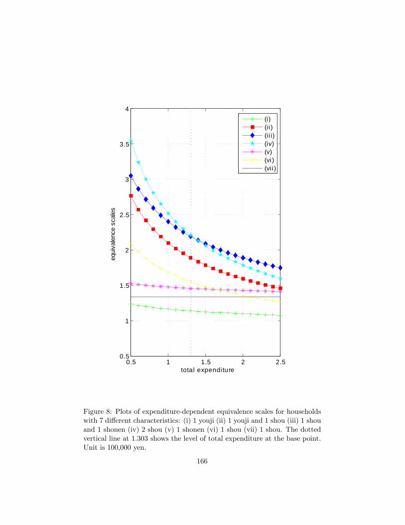
0.5 1 1.5 2 2.50.5
1
1.5
2
2.5
3
3.5
4
total expenditure
equi
vale
nce
scal
es(i )(i i )(i i i)(iv)(v)(vi)(vi i)
Figure 8: Plots of expenditure-dependent equivalence scales for householdswith 7 di¤erent characteristics: (i) 1 youji (ii) 1 youji and 1 shou (iii) 1 shouand 1 shonen (iv) 2 shou (v) 1 shonen (vi) 1 shou (vii) 1 shou. The dottedvertical line at 1:303 shows the level of total expenditure at the base point.Unit is 100,000 yen.
166
dren should consider the progressivity in the compensation. Poor households
with children should be given bigger compensations than rich households
with children to maintain the welfare equality. However, the lack of stronger
degrees of decline in the equivalence scales as income rises and their statisti-
cal signi�cance weaken the above assertion since our estimated equivalence
scales still produce higher equivalent expenditures for higher-income class
households.
167
5. Conclusion
In this dissertation, after reviewing relevant theoretical results on the con-
sumer demand theory in chapter 2, chapter 3 investigates the regularity
property of the normalized quadratic demand system of Diewert and Wales
(1988b). The regularity conditions of monotonicity and concavity are two
of the axioms which guarantee the existence of the utility maximizing con-
sumers, and the ful�llment of all axioms makes direct utility, indirect util-
ity, and expenditure functions equivalent representations of the underlying
preferences. Without satisfaction of both curvature and monotonicity, the
second-order condition for optimizating behavior fails, duality theory fails,
and inferences resulting from derived estimating equations become invalid.
Barnett (2002) commented that imposition of the monotonicity condition is
especially overlooked when global curvature is imposed on the NQ model.
To futher examine his observation, we displayed regular regions, di¤eren-
tiating regular and non-regualr regions by the types of violations to fully
reveal the regularity property of the NQ model. We tried three methods of
imposing curvature on the NQ model: global, local, and no curvature im-
position, to see how the di¤erent methods a¤ect the regular regions of the
model. We found that monotonicity violations are especially likely to occur
when elasticities of substitution are greater than one. We also found that
imposing curvature locally produces di¢ culties in estimation, smaller regu-
lar regions, and poor elasticity estimates in many cases considered. When
imposing curvature globally, our results were better. Although violations of
monotonicity remained common in some of our cases, those violations do not
168
appear to have been induced solely by the curvature imposition, but rather
by the nature of the Normalized Quadratic model itself. However, impo-
sition of global curvature makes complement goods more complement and
substitute goods more substitute. With the Normalized Quadratic model,
we �nd that both curvature and monotonicity must be checked with the
estimated model, as has previously been shown to be the case with many
other �exible functional forms. Imposition of curvature alone does not as-
sure regularity, and imposing local curvature alone can have very adverse
consequences.
One straightforward future research direction is to expand the analysis
to other, even newer demand systems such as QUAIDS, which has been
increasingly used as a better alternative to the classic AIDS model, and
such as the translated QUAIDS, which has the unusually high rank of four.
Lewbel (1988) suggested that a rank-three trigonometric demand system is
able to produce an unusually large regular region, but its implementation is
only found in Matsuda (2006) as far as we know.
Another direction is to try di¤erent methods of imposing correct curva-
ture on demand functions. Diewert and Lawrence (2002) proposed imposing
curvature at two points to ensure globally correct curvature without sacri-
�cing the �exibility property of the normalized quadratic pro�t function.
Diewert and Wales (1988a) proposed the concept of a semi�exible func-
tional form in which the rank of the Slutsky matrix is reduced, but in a
manner that does not restrict the price derivatives in any a priori undesir-
able way. This allows the researcher to systematically limit the parameter
space while maintaining full income �exibility and partial price �exibility,
169
an objective that may prove useful in large demand systems. The model is
designed to estimate large demand systems by sacri�cing the �exibility to
attain globally correct curvature (Ryan and Wales, 1998). Moschini (1998)
studied the semi�exible AIDS on which only the local curvature is imposed.
Thus, it may be interesting to see whether this additional restrictiveness
induces further monotonicity violations as the rank of the Slutsky matrix is
reduced.
In chapter 4, we studied the expenditure-dependent equivalence scales to
estimate the cost of a child in Japan. We found that the Japanese household
equivalence scales are decreasing in the total expenditure as well as increas-
ing in the number of children. We introduced the property called "Gener-
alized Relative/Absolute Expenditure-Scale Exactness" (GRESE/GAESE)
which can identify the estimated equivalence scales by observed demand data
alone if the speci�cation of the reference household expenditure function is
neither a¢ ne nor log-a¢ ne (PIGLOG). Hence, we employ the functional
forms of the demand model that are neither a¢ ne nor log-a¢ ne and that
have a higher rank which can explain the more complicated shapes of the
Engel curves. We paid special attention to correcting a possible bias in the
parameter estimation induced by a pile of observations of zero expenditure
on some goods. Our results suggest an intuitively straightfoward policy
design for the child-support welfare program: the compensation should de-
pend on their income level as well as on the number of children. Depending
on what type of health insurance a household holds, Japan�s current child-
subsidy program sets income threshold levels for receiving child-support in
the form of monetary compensation. But the new recently proposed pro-
170
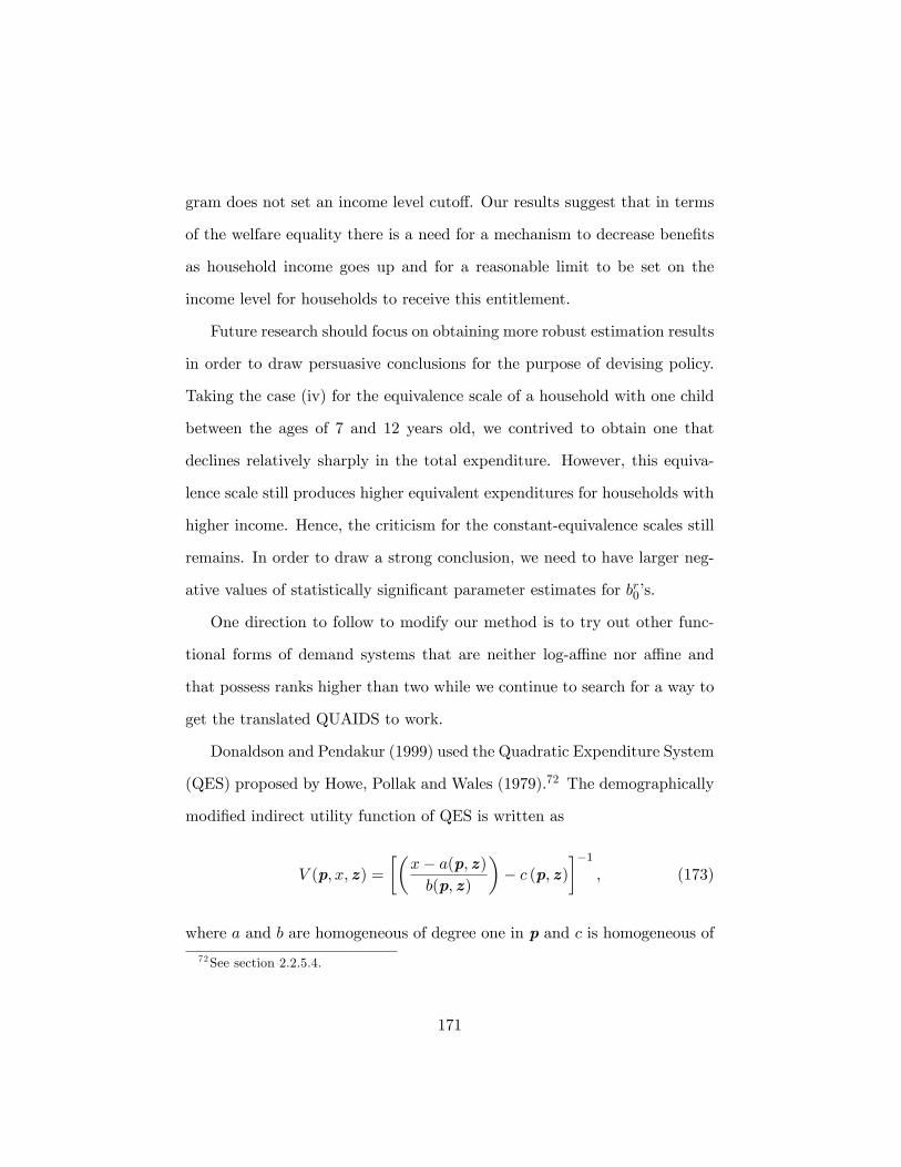
gram does not set an income level cuto¤. Our results suggest that in terms
of the welfare equality there is a need for a mechanism to decrease bene�ts
as household income goes up and for a reasonable limit to be set on the
income level for households to receive this entitlement.
Future research should focus on obtaining more robust estimation results
in order to draw persuasive conclusions for the purpose of devising policy.
Taking the case (iv) for the equivalence scale of a household with one child
between the ages of 7 and 12 years old, we contrived to obtain one that
declines relatively sharply in the total expenditure. However, this equiva-
lence scale still produces higher equivalent expenditures for households with
higher income. Hence, the criticism for the constant-equivalence scales still
remains. In order to draw a strong conclusion, we need to have larger neg-
ative values of statistically signi�cant parameter estimates for br0�s.
One direction to follow to modify our method is to try out other func-
tional forms of demand systems that are neither log-a¢ ne nor a¢ ne and
that possess ranks higher than two while we continue to search for a way to
get the translated QUAIDS to work.
Donaldson and Pendakur (1999) used the Quadratic Expenditure System
(QES) proposed by Howe, Pollak and Wales (1979).72 The demographically
modi�ed indirect utility function of QES is written as
V (p; x;z) =
��x� a(p;z)b(p;z)
�� c (p;z)
��1, (173)
where a and b are homogeneous of degree one in p and c is homogeneous of
72See section 2.2.5.4.
171
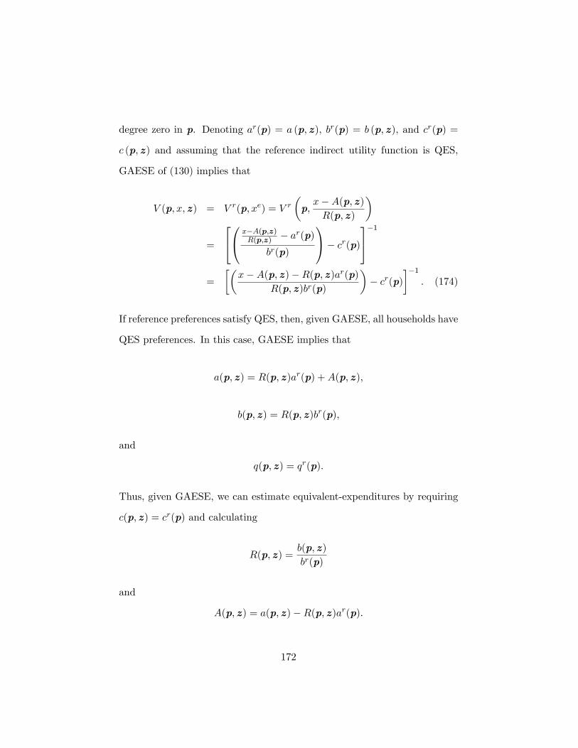
degree zero in p. Denoting ar(p) = a (p;z), br(p) = b (p;z), and cr(p) =
c (p;z) and assuming that the reference indirect utility function is QES,
GAESE of (130) implies that
V (p; x;z) = V r(p; xe) = V r�p;x�A(p;z)R(p;z)
�
=
240@ x�A(p;z)R(p;z) � ar(p)
br(p)
1A� cr(p)35�1
=
��x�A(p;z)�R(p;z)ar(p)
R(p;z)br(p)
�� cr(p)
��1. (174)
If reference preferences satisfy QES, then, given GAESE, all households have
QES preferences. In this case, GAESE implies that
a(p;z) = R(p;z)ar(p) +A(p;z);
b(p;z) = R(p;z)br(p),
and
q(p;z) = qr(p).
Thus, given GAESE, we can estimate equivalent-expenditures by requiring
c(p;z) = cr(p) and calculating
R(p;z) =b(p;z)
br(p)
and
A(p;z) = a(p;z)�R(p;z)ar(p).
172
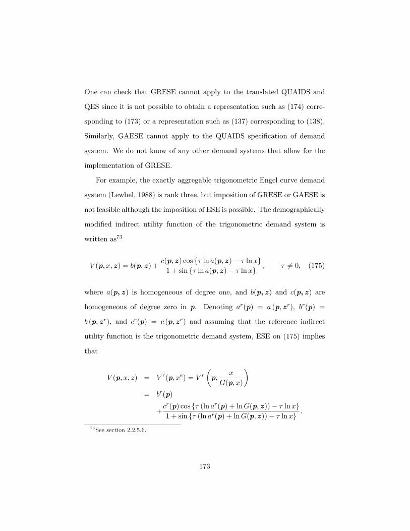
One can check that GRESE cannot apply to the translated QUAIDS and
QES since it is not possible to obtain a representation such as (174) corre-
sponding to (173) or a representation such as (137) corresponding to (138).
Similarly, GAESE cannot apply to the QUAIDS speci�cation of demand
system. We do not know of any other demand systems that allow for the
implementation of GRESE.
For example, the exactly aggregable trigonometric Engel curve demand
system (Lewbel, 1988) is rank three, but imposition of GRESE or GAESE is
not feasible although the imposition of ESE is possible. The demographically
modi�ed indirect utility function of the trigonometric demand system is
written as73
V (p; x;z) = b(p;z) +c(p;z) cos f� ln a(p;z)� � lnxg1 + sin f� ln a(p;z)� � lnxg , � 6= 0, (175)
where a(p; z) is homogeneous of degree one, and b(p; z) and c(p; z) are
homogeneous of degree zero in p. Denoting ar(p) = a (p;zr), br(p) =
b (p;zr), and cr(p) = c (p;zr) and assuming that the reference indirect
utility function is the trigonometric demand system, ESE on (175) implies
that
V (p; x; z) = V r(p; xe) = V r�p;
x
G(p; x)
�= br(p)
+cr(p) cos f� (ln ar(p) + lnG(p;z))� � lnxg1 + sin f� (ln ar(p) + lnG(p;z))� � lnxg :
73See section 2.2.5.6.
173
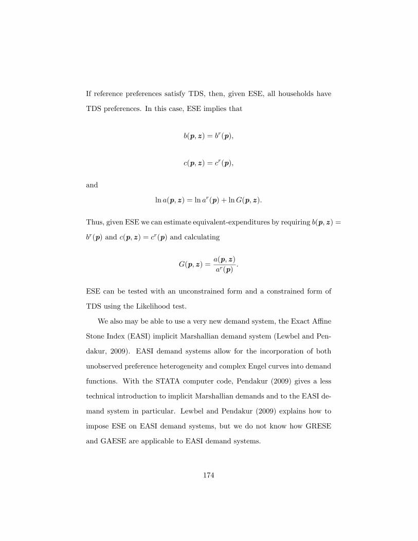
If reference preferences satisfy TDS, then, given ESE, all households have
TDS preferences. In this case, ESE implies that
b(p;z) = br(p);
c(p;z) = cr(p);
and
ln a(p;z) = ln ar(p) + lnG(p;z).
Thus, given ESE we can estimate equivalent-expenditures by requiring b(p;z) =
br(p) and c(p;z) = cr(p) and calculating
G(p;z) =a(p;z)
ar(p).
ESE can be tested with an unconstrained form and a constrained form of
TDS using the Likelihood test.
We also may be able to use a very new demand system, the Exact A¢ ne
Stone Index (EASI) implicit Marshallian demand system (Lewbel and Pen-
dakur, 2009). EASI demand systems allow for the incorporation of both
unobserved preference heterogeneity and complex Engel curves into demand
functions. With the STATA computer code, Pendakur (2009) gives a less
technical introduction to implicit Marshallian demands and to the EASI de-
mand system in particular. Lewbel and Pendakur (2009) explains how to
impose ESE on EASI demand systems, but we do not know how GRESE
and GAESE are applicable to EASI demand systems.
174

Another direction to improve our procedure is to try out di¤erent meth-
ods to address the presence of a pile of zero-expenditure observations on
some goods. Hasegawa, Ueda and Mori (2008) explicitly assume the mecha-
nism of a number of the zero expenditure occurrence as infrequency of pur-
chase (IFP), and they estimate a system of Engel functions using Markov
chain Monte Carlo method to obtain the estimates of unobservable para-
meters. Golan, Perlo¤ and Shen (2001) demonstrate a new approach to
e¢ ciently estimate a system of AIDS demand functions for Mexican meat
demand with binding nonnegativity constraints. This approach, called gen-
eralized maximum entropy (GME) building on the entropy-information mea-
sure of Shannon (1948), the classical maximum entropy (ME) principle of
Jaynes (1957a, 1957b) which was developed to recover information from un-
derdetermined systems, and generalized maximum entropy theory of Golan,
Judge and Miller (1996), is more practical and e¢ cient than traditional
maximum likelihood methods. The methods have been applied in Golan,
Judge and Miller (2003); Golan, Judge and Karp (1996); and Arndt (1999).
The implementation of these innovative procedures is technically di¢ cult
and computationally intensive. In any case, the ideal method will be the
one that can utilize the household characteristic e¤ects most e¤ectively. The
procedure in chapter 4 conveniently assumes that the explanatory variables
of sample selection equations are any possible demographic characteristics
variables other than prices, total expenditures, and the number of age types
of the children. It is possible that some of the demographic characteristics
variables may better explain the household behavior if included in the de-
mand system. Another improvement will be to use the multivariate Probit
175

model instead of the Probit estimation of each share equation to increase
the e¢ ciency of the �rst-step estimation procedure.
We may even be able to exploit the nature of our data set as panel data
to avoid using any of the restrictive GRESE or GAESE to construct the
expenditure-dependent equivalence scales. It is possible to incorporate un-
observable individual heterogeneity into demand systems as random e¤ects
(Pollak and Wales, 1992, ch.5) or to use the EASI demand system which al-
ready has embeded the feature.74 But we are not aware of any studies which
successfully take advantage of panel data as "additional data" to identify
the expenditure-dependent equivalence scales and which address the zero
expenditure issue at the same time.
74Biørn and Jansen (1983) estimated a system of demand functions with individuale¤ects using incomplete cross-section/time-series data.
176
References
[1] Abe, A. (2003), "E¤ects of child-related bene�ts in Japan," TheJapanese Journal of Social Security Policy, 1, 51-59.
[2] Aitchison, J. and J.A.C. Brown (1954-5), "A Synthesis of Engel CurveTheory," Review of Economic Studies, 22, 35-46.
[3] Allen, G.D., and J.R. Hicks (1934), "A Reconsideration of the Theoryof Value, Part II," Economica, 1, 196-219.
[4] Aneuryn-Evans, G. B. and A. S. Deaton (1980), "Testing Linear versusLogarithmic Regressions," Review of Economic Studies, 47, 275-91.
[5] Aoki, R., and Y. Konishi (2009a), "On the Persistence of LowBirthrate in Japan," PIE Discussion Paper, Institute of Economic Re-search, Hitotsubashi University.
[6] Aoki, R., and Y. Konishi (2009b), "Relationship between Consump-tion, Labor Supply and Fertility � Theory and Evidence from Japan,"PIE Discussion Paper, Institute of Economic Research, HitotsubashiUniversity.
[7] Arndt, C. (1999), "Demand for Herbicide in Corn: An Entropy Ap-proach Using Micro-level Data," Journal of Agricultural and ResourceEconomics 24, 204-221.
[8] Arrow, K.J. and A.C. Enthoven (1961), "Quasi-concave Program-ming," Econometrica 29, 779-800.
[9] Banks, J., R. Blundell and A. Lewbel (1997), "Quadratic Engel Curvesand Consumer Demand," Review of Economics and Statistics 79, 527-539.
[10] Barnett, W.A. (1977), "Recursive subaggregation and a generalizedhypocycloidal demand model, Econometrica," 45, 1117�1136.
[11] Barnett, W.A. (1979), "The Joint Allocation of Leisure and GoodsExpenditure," Econometrica, 47, 539-563. (Reprinted in FunctionalStructure and Approximation in Econometrics, W.A. Barnett, andJ.M. Binner (eds.), 2004, Chapter 2, Amsterdam, Elsevier).
[12] Barnett, W.A. (1981), Consumer Demand and Labor Supply, (Horth-Holand, Amsterdam).
177
[13] Barnett, W.A. (1983a), "New Indices of Money Supply and the Flex-ible Laurent Demand System," Journal of Business and EconomicStatistics, 1, 7-23 (Reprinted in The Theory of Monetary Aggrega-tion, W.A. Barnett and A. Serletis (eds.), 2000, Chapter 16. Elsevier:North-Holland).
[14] Barnett, W.A. (1983b), "De�nitions of Second Order Approxima-tion and of Flexible Functional Form," Economics Letters, 12, 31-35(Reprinted in Functional Structure and Approximation in Economet-rics, W.A. Barnett, and J.M. Binner (eds.), 2004, Chapter 3, Amster-dam, Elsevier).
[15] Barnett, W.A. (2002), "Tastes and Technology: Curvature is NotSu¢ cient for Regularity," Journal of Econometrics, 108, 199-202(Reprinted in Functional Structure and Approximation in Economet-rics, W.A. Barnett, and J.M. Binner (eds.), 2004, Chapter 17, Ams-terdam, Elsevier).
[16] Barnett, W.A. and S. Choi (1989), "A Monte Carlo Study of Testsof Blockwise Weak Separability," Journal of Business and EconomicStatistics, 7, 363-377 (Reprinted in Functional Structure and Approx-imation in Econometrics, W.A. Barnett, and J.M. Binner (eds.), 2004,Chapter 12, Amsterdam, Elsevier).
[17] Barnett, W.A. and A. Jonas (1983), "The Müntz-Szatz Demand Sys-tem: An Application of a Globally Well Behaved Series Expansion.Economics Letters, 11, 337-342 (Reprinted in Functional Structureand Approximation in Econometrics, W.A. Barnett, and J.M. Binner(eds.), 2004, Chapter 8, Amsterdam, Elsevier).
[18] Barnett, W.A. and Y.W. Lee (1985), "The Global Properties of theMin�ex Laurent, Generalized Leontief, and Translog Flexible Func-tional Forms," Econometrica, 53, 1421-1437 (Reprinted in FunctionalStructure and Approximation in Econometrics, W. A. Barnett, and J.M. Binner (eds.), 2004, Chapter 4, Amsterdam, Elsevier).
[19] Barnett, W.A., Lee, Y.W. and M.D. Wolfe (1985), The three-dimensional global properties of the Min�ex Laurent, generalizedLeontief, and translog �exible functional forms. Journal of Economet-rics, 30, 3-31 (Reprinted in Functional Structure and Approximation inEconometrics, W. A. Barnett, and J. M. Binner (eds.), 2004, Chapter6, Amsterdam, Elsevier).
178
[20] Barnett, W. A., Y.W. Lee and M.D. Wolfe (1987), "The Global Prop-erties of the Two Min�ex Laurent Flexible Functional Forms," Jour-nal of Econometrics, 36, 281-298 (Reprinted in Functional Structureand Approximation in Econometrics, W.A. Barnett, and J.M. Binner(eds.), 2004, Chapter 7, Amsterdam, Elsevier).
[21] Barnett, W.A., J. Geweke and M. Wolfe (1991a), "Semiparamet-ric Bayesian Estimation of Applied General Equilibrium Models," inEquilibrium Theory and Applications, Proceedings of the Sixth Inter-national Symposium in Economic Theory and Econometrics, W.A.Barnett, A. Mas-Colell, J. Drèze, C. D�Aspremont and B.Cornet(eds.), Cambridge, MA: Cambridge University Press, 425-480.
[22] Barnett, W.A., J. Geweke and M. Wolfe (1991b), "SemiparametricBayesian Estimation of the Asymptotically Ideal Production Model,"Journal of Econometrics, 49, 5-50 (Reprinted in Functional Structureand Approximation in Econometrics, W.A. Barnett, and J.M. Binner(eds.), 2004, Chapter 14, Amsterdam, Elsevier).
[23] Barnett, W.A., K.J. Kopecky and R. Sato (1981), "Estimation of Im-plicit Utility Models," European Economics Review, 15, 247-259.
[24] Barnett, W.A., M. Kirova and M. Pasupathy (1995), "Estimating Pol-icy Invariant Deep Parameters in the Financial Sector When Risk andGrowth Matter," Journal of Money, Credit and Banking, 27, 1402-1430 (Reprinted in The Theory of Monetary Aggregation, W. A. Bar-nett, and A. Serletis (eds.), 2000, Chapter 22, North Holland).
[25] Barnett, W.A. and M. Pasupathy (2003), "Regularity of the Gener-alized Quadratic Production Model: Counterexample," EconometricReview, 22(2), 135-154.
[26] Barnett, W.A. and O. Seck (2008), "Rotterdam Model versus AlmostIdeal Demand System: Will the Best Speci�cation Please Stand Up?"Journal of Applied Econometrics, 23, 795-824.
[27] Barnett, W.A. and A. Serletis (2008), "Consumer Preferences andDemand Systems," Journal of Econometrics, 147, 210-224.
[28] Barnett, W.A. and A. Serletis (2009), "Measuring Consumer Prefer-ences and Estimating Demand Systems," Chapter 1 in Contributionsto Economics Analysis, Daniel Slottje (eds.), Emerald Group Publish-ing Limited, 288, 1-35.
179
[29] Barnett, W.A. and Usui, I. (2007), "The Theoretical RegularityProperties of the Normalized Quadratic Consumer Demand Model,"Functional Structure Inference, W.A. Barnett and A. Serletis (eds.),Amsterdam:North-Holland, 1994.
[30] Barten, A.P. (1966), "Theorie en empirie van een volledig stelsel vanvraagvergelijkingen (Theory and empirics of a complete system of de-mand equation)," Doctoral dissertation (Netherlands School of Eco-nomics, Rotterdam).
[31] Barten, A.P. (1969), "Maximum Likelihood Estimation of a CompleteSystem of Demand Equations," European Economic Review 1, 7-73.
[32] Basmann, R.L., D.J. Molina and D.J. Slottje (1983), "Budget Con-straint Prices as Preference Changing Parameters of GeneralizedFechner-Thurstone Direct Utility Functions," American Economic Re-view 73, 411-413.
[33] Basmann, R.L., C.A. Diamond, J.C. Frentrup and S.N. White (1985),"On Deviations Between Neoclassical and GFT-Based True Cost-of-Living Indexes Derived From the Same Demand Function System,"Journal of Econometrics 30, 45-66 (Reprinted in New Approaches toModeling, Speci�cation Selection, and Econometric Inference, W. A.Barnett, and A. R. Gallant (eds.), 1989, Cambridge University Press,Cambridge, 45-66).
[34] Basmann, R.L., C. Fawson and R.C. Shumway (1990), "AgriculturalProduction Technologies with Systematic and Stochastic TechnicalChange," American Journal of Agricultural Economics 72, 182-199.
[35] Basmann, R.L., K.J. Hayes and D.J. Slottje (1994), "Testing an Al-ternative Habit Persistence Model," Southern Economic Journal 60,739-753.
[36] Berndt, E.R. and L.R. Christensen (1973), "The Translog Functionand the Substitution of Equipment, Structures and Labor in U.S. Man-ufacturing, 1992-1968," Journal of Econometrics, 1, 81-114.
[37] Berndt, E.R. and L.R. Christensen (1974), "Testing for the Existenceof a Consistent Aggregate Index of Labor Inputs," American EconomicReview, 64, 391-404.
180
[38] Berndt, E.R. and D.O. Wood (1975), "Technology, Prices, and theDerived Demand for Energy," Review of Economics and Statistics, 43,259-268.
[39] Berndt, E.R. and M.S. Khaled (1979), "Parametric Productivity Mea-surement and Choice among Flexible Functional Forms,"Journal ofPolitical Economy 87, 1220�1245.
[40] Biørn, E. and E.S. Jansen (1983), "Individual E¤ects in a System ofDemand Functions," Scandinavian Journal of Economics, 85, 461-483.
[41] Blackorby, C., D. Primont and R.R. Russell (1977), "On TestingSeparability Restrictions with Flexible Functional Forms," Journal ofEconometrics 5, 195-209.
[42] Blackorby, C., D. Primont, D. and R.R. Russell (1978), Duality, Sep-arability, and Functional Structure, Amsterdam: North-Holland.
[43] Blackorby, C. and R. R. Russell (1981), "The Morishima Elasticityof Substitution: Symmetry, Constancy, Separability, and Its Relation-ship to the Hicks and Allen Elasticities," Review of Economic Studies48, 147�158.
[44] Blackorby, C. and R.R. Russell (1989), "Will the Real Elasticity ofSubstitution Please Stand Up? (A Comparison of the Allen/Uzawaand Morishima elasticities)," American Economic Review 79, 882-888.
[45] Blackorby, C. and D. Donaldson (1991), "Adult-Equivalence Scales,Interpersonal Comparisons of Well-Being, and Applied Welfare Eco-nomics," in Interpersonal Comparisons and Distributive Justice, (eds).J. Elster and J. Roemer, Cambridge, U.K.: Cambridge UniversityPress, 164-199.
[46] Blackorby, C. and D. Donaldson (1993), "Adult-Equivalence Scalesand the Economic Implementation of Interpersonal Comparisons ofWell-Being," Social Choice and Welfare, 10, 335�361.
[47] Blackorby, C. and D. Donaldson (1994), "Measuring the Cost of Chil-dren: A Theoretical Framework," in The Measurement of HouseholdWelfare, (eds.) R. Blundell, I. Preston, and I. Walker, Cambridge,U.K.: Cambridge University Press, 51�69.
181
[48] Blackorby, C., W. Schworm and T. Fisher (1986), "Testing for theExistence of Input Aggregates in an Economy Production Function,"Discussion Paper no.8646 (CORE, Université Catholique de Louvain,Louvain).
[49] Blundell, R. (1988), "Consumer behavior: Theory and Empirical Ev-idence � A Survey," Economic Journal 98, 16-65.
[50] Blundell, R., X. Chen and D. Kristensen (2007), "Semi-NonparametricIV Estimation of Shape-Invariant Engel Curves," Econometrica, 75,1613-1669.
[51] Blundell R., R. Duncan and K. Pendakur (1998), "SemiparametricEstimation and Consumer Demand," Journal of Applied Econometrics13, 435-461.
[52] Blundell, R. and C. Meghir (1987), "Bivariate Alternatives to theTobit model," Journal of Econometrics, 34, 179�200.
[53] Blundell, R. and A. Lewbel (1991), "The Information Content ofEquivalence Scales," Journal of Econometrics, 50, 49�68.
[54] Brown, J. A. and A. Deaton (1972), "Methods of Consumer behavior:A Survey," Economic Journal, 82, 1145-1236.
[55] Browning, M. (1992), "Children and Household Economic Behavior,"Journal of Economic Literature 30, 1434�1475.
[56] Caves, D.W. and L.R. Christensen, (1980), "Global Properties of theFlexible Functional Forms," American Economic Review 70, 422-432.
[57] Christensen, L.R., D.W. Jorgenson and L.J. Lau (1971), "Transce-dental Logarithmic Production Frontiers," Review of Economics andStatistics 55, 28-45.
[58] Christensen, L.R., D.W. Jorgenson, and L.J. Lau, (1975), "Transcen-dental Logarithmic Utility Functions," American Economic Review65, 367-383.
[59] Conni¤e, D. (1992), "The Non-Constancy of Equivalence Scales," Re-view of Income and Wealth, 4, 429-43.
[60] Cook, P.J. (1972), "A �One Line� Proof of the Slutsky Equation,"American Economic Review, 62, 139.
182
[61] Cooper, R.J. and K.R. McLaren, (1992) "An Empirically OrientedDemand System with Improved Regularity Properties, " CanadianJournal of Economics, 25, 652-667.
[62] Cooper, R.J. and K.R. McLaren (1996), "A System of Demand Equa-tions Satisfying E¤ectively Global Regularity Conditions," Review ofEconomics and Statistics 78, 359-364.
[63] Date, Y. and S. Shimizutani (2007), "Why Has Japan�s Fertility RateDeclined?: An Empirical Literature Survey with an Emphasis on Pol-icy Implications," Japanese Economy, M.E. Sharpe, Inc., 34, 4-45.
[64] Davis, G.C. and J. Gauger (1996), "Measuring Substitution in Mone-tary Asset Demand Systems," Journal of Business and Economic Sta-tistics 14, 203-208.
[65] Deaton, A. (1986), Demand Analysis, Ch. 30 of Handbook of Econo-metrics, Volume III, edited by Z. Griliches and M.D. Intrilligator.North-Holland, New York, 1767-1839.
[66] Deaton, A. (1997), Analysis of Household Surveys, Baltimore MD:Johns Hopkins University Press.
[67] Deaton, A. and Irish, M. (1984), "Statistical Models for Zero Expendi-tures in Household Budgets," Journal of Public Economics, 23, 59�80.
[68] Deaton, A. and Muellbauer, J. (1980), "An Almost Ideal DemandSystem," American Economic Review 70, 312-326.
[69] Deaton, A. and J. Muellbauer, (1980b), Economics and consumer be-havior. Cambridge University Press, Cambridge.
[70] Debreu, G. (1960), "Topological Methods in Cardinal Utility Theory,"In Mathematical Methods in the Social Sciences, 1959, edited by Ken-neth J. Arrow, Samuel Karlin, and Patrick Suppes, 16-26. Stanford:Stanford University Press.
[71] Denny, M. and M. Fuss (1977), "The Use of Approximation Analysisto Test for Separability and the Existence of Consistent Aggregates,"American Economic Review, 67, 404-418.
[72] De Peretti, P. (2005), "Testing the Signi�cance of the Departures fromUtility Maximization," Macroeconomic Dynamics 9, 372-397.
183
[73] Dickens, R., V. Fry and P. Pashardes (1993), Nonlinearities, Aggrega-tion and Equivalence Scales," Economic Journal 103, 359�368.
[74] Diewert, W.E. (1971), "An Application of the Shephard Duality Theo-rem: a Generalized Leontief Production Function," Journal of PoliticalEconomy 79, 481-507.
[75] Diewert, W.E. (1973), "Functional Forms for Pro�t and Transforma-tion Functions," Journal of Economic Theory 6, 284-316.
[76] Diewert, W.E. (1974). "Applications of Duality Theory," in Frontiersof Quantitative Economics, M. D. Intriligator and D. A. Kendrick(eds.), vol. 2, Amsterdam: North-Holland, 106-171.
[77] Diewert, W.E. (1982), "Duality Approaches to Microeconomic The-ory," in Kenneth J. Arrow and Michael D. Intriligator (eds.), Hand-book of Mathematical Economics, vol. II (Amsterdam: North-Holland).
[78] Diewert, W.E. and D. Lawrence (2002), "The Deadweight Costs ofCapital Taxation in Australia," in E¢ ciency in the Public Sector,Kevin J. Fox (ed.), Boston: Kluwer Academic Publishers, 103-167.
[79] Diewert, W.E. and T.J. Wales (1987), "Flexible Functional Forms andGlobal Curvature Conditions," Econometrica 55, 43-68.
[80] Diewert, W.E. and T.J. Wales (1988a), "A Normalized QuadraticSemi�exible Functional Form," Journal of Econometrics 37, 327-342.
[81] Diewert, W.E. and T.J. Wales (1988b), "Normalized Quadratic Sys-tems of Consumer Demand Functions," Journal of Business and Eco-nomic Statistics 6, 303-312.
[82] Diewert, W.E. and T.J. Wales (1992), "Quadratic Spline Models forProducer Supply and Demand Functions," International Economic Re-view 33, 705-722.
[83] Diewert, W.E. and T.J. Wales (1993), Linear and Quadratic SplineModels for Consumer Demand Functions," Canadian Journal of Eco-nomics 26, 77-106.
[84] Diewert, W.E. and T.J. Wales (1995), Flexible Functional Forms andTests of Homogeneous Separability," Journal of Econometrics 67, 259-302.
184
[85] Diewert, W.E. and K.J. Fox (1999), "Is the Asia-paci�c region dif-ferent? Technical progress bias and price elasticity estimates for 18OECD countries, 1960-1992," in Economic E¢ ciency and Productiv-ity Growth in the Asia-Paci�c Region, T-T. Fu, C. J. Huang and C. A.K. Lovell (eds.), Cheltenham and Northampton, UK: Edward ElgarPublishing, 125-144.
[86] Donald, S.G. (1997), "Inference Concerning the Number of Factorsin a Multivariate Nonparametric relationship," Econometrica 65, 103-132.
[87] Donaldson, D. and K. Pendakur (1999), "Equivalent-Income Functionsand Income-Dependent Equivalence Scales," Discussion Paper, SimonFraser University.
[88] Donaldson, D. and K. Pendakur (2004), "Equivalent-ExpenditureFunctions and Expenditure-Dependent Equivalence Scales," Journalof Public Economics, 88, 175�208.
[89] Donaldson, D. and K. Pendakur (2006) "The Identi�cation of FixedCosts from Consumer Behavior," Journal of Business and EconomicStatistics, 24, 255-265.
[90] Dorsey, R.E. and W.J. Mayer (1995), "Genetic Algorithms for Estima-tion Problems with Multiple Optima, Nondi¤erentiability, and OtherIrregular Features," Journal of Business and Economic Statistics 13,53-66.
[91] Ebert, U. and P. Moyes (2003), "Equivalence Scales Revisited," Econo-metrica, 71, 319�344.
[92] Fisher, D., and A.R. Fleissig (1996), "Monetary Aggregation and theDemand for Assets," Journal of Money, Credit and Banking, 29, 371-380.
[93] Fleissig, A.R. and J. Swo¤ord (1996), "A Dynamic AsymptoticallyIdeal Model of Money Demand," Journal of Monetary Economics, 37,371-380.
[94] Fleissig, A.R., T. Kastens and D. Terrell (2000), "Evaluating the Semi-nonparametric Fourier, AIM, and Neural Networks Cost Functions,"Economics Letters 68, 235-244.
185
[95] Fleissig, A.R. and G.A. Whitney (2003), "A New PC-Based Test forVarian�s Weak Separability Conditions," Journal of Business and Eco-nomics Statistics, 21, 133-144.
[96] Frenger, P. (1978), "Factor Substitution in the Interindustry Modeland the Use of Inconsistent Aggregation," in M. Fuss and D. McFad-den, (eds), vol.2, 269-310.
[97] Frenger, P. (1985a), "The Concavity of the Cost Function and Estima-tion of the Shadow Elasticity of Substitution, Discussion paper, no.7(Central Bureau of Statistics, Oslo).
[98] Frenger, P. (1985b), "Using the Directional Shadow Elasticity of Sub-stitution to Measure the Concavity of the Cost Function," EconomicsLetters, 19, 171-175.
[99] Fry, V. and P. Pashardes (1994), "Abstention and Aggregation in Con-sumer Demand: Zero Tobacco Expenditures," Oxford Economic Pa-pers, 46, 502-518.
[100] Gallant, A.R. (1981), "On the Bias in Flexible Functional Forms andan Essentially Unbiased Form: the Fourier Flexible Form," Journal ofEconometrics 1, 211-245.
[101] Gallant, A.R. and G.H. Golub (1984), "Imposing Curvature Restric-tions on Flexible Functional Forms," Journal of Econometrics 267,295-321.
[102] Gill, L. and A. Lewbel (1992), "Testing the Rank of Estimated Ma-trices with Applications to Factor, State Space, and ARMA Models,"Journal of the American Statistical Association 87, 766-776.
[103] Golan, A., M.P. Je¤rey and E.Z. Shen (2001), "Estimating a DemandSystem with Nonnegativity Constraints: Mexican Meat DemandAu-thor," The Review of Economics and Statistics, 83, 541-550.
[104] Golan, A., G. Judge and L. Karp (1996), "A Maximum Entropy Ap-proach to Estimation and Inference in Dynamic Models or CountingFish in the Sea Using Maximum Entropy," Journal of Economic Dy-namics and Control, 20, 559-582.
[105] Golan, A., G. Judge, and D. Miller (1996), Maximum Entrop Econo-metrics: Robust Estimation With Limited Data, New York: JohnWiley Sons.
186
[106] Golan, A. and J.M. Perlo¤ (2002), "Comparison of Maximum Entropyand Higher-Order Entropy Estimators," Journal of Econometrics, 107,195-211.
[107] Goldman, S.M. and H. Uzawa (1964), "A Note on Separability inDemand Analysis," Econometrica 32, 387-398.
[108] Gorman, W.M. (1953), "Community Preference Fields," Economet-rica, 21, 63-80.
[109] Gorman, W.M. (1959), "Separable Utility and Aggregation," Econo-metrica 27, 469-481.
[110] Gorman, W.M. (1961), "On a Class of Preference Fields," Metroeco-nomica 13, 53-56.
[111] Gorman, W.M. (1971a), "Apologia for a Lemma, Review of EconomicStudies," 35, 367-390.
[112] Gorman, W.M. (1971b), "Clontarf Revisited, Review of EconomicStudies," 38, 116.
[113] Gorman, W.M. (1975), "Tricks with Utility Functions," in M. J. Artisand A. R. Nobay, (eds.), Essays inEconomic Analysis: Proceedings ofthe 1975 AUTE Confetence, She¢ eld (Cambridge: Cambridge Uni-versity Press), 211-243.
[114] Gorman, W.M. (1981), "Some Engel curves," in: A.S. Deaton, (ed.),Essays in the theory and measurement of consumer behavior: In hon-our of Sir Richard Stone. CambridgeUniversity Press, Cambridge.
[115] Gozalo, P. (1997), "Nonparametric Bootstrap Analysis with Applica-tions to Demographic E¤ects in Demand Functions," Journal of Econo-metrics 81, 357�393.
[116] Cragg, J. G. and S.G. Donald (1997), "Inferring the Rank of a Matrix,"Journal of Econometrics, 76, 223-250.
[117] Gri¢ ths, W. and M.R. Valenzuela (1998), "Missing Data From Infre-quency of Purchase: Bayesian Estimation of a Linear Expenditure Sys-tem," in Fomby T. B. and Hill R. C. (eds.), Advances in Econometrics:Messy Data �Missing Observations, Outliers, and Mixed-FrequencyData, Vol. 13, JAI Press, Greenwich, 75�102.
187
[118] Grodal, B. and W. Hildenbrand (1992), "Cross Section Engel Curves,Expenditure Distributions and the Law of Demand," In: Phlips L,Taylor LD (eds.) Essays in honor of H. S. Houthakker. Kluwer, Dor-drecht, 85-120.
[119] Gronau, R. (1988), "Consumption Technology and the IntrafamilyDistribution of Resources: Adult Equivalence Scales Reexamined,"Journal of Political Economy, 96, 1183-1205.
[120] Guilkey, D.K. and C.A.K Lovell (1980), "On the Flexibility of theTranslog Approximation," International Economic Review 21, 137-147.
[121] Guilkey, D.K., C.A.K. Lovell and R.C. Sickles (1983), "A Comparisonof the Performance of Three Flexible Functional Forms," InternationalEconomic Review 24, 591-616.
[122] Hanoch, G. (1975), "Production and Demand Model with Direct andIndirect Implicit Additivity," Econometrica 45, 395-419.
[123] Hardy, G.F., L.E. Littlewood and G. Polya (1952), Inequalities, (Cam-bridge: Cambridge University Press).
[124] Hausman, J.A., W.K. Newey and J.L. Powell (1995), "Nonlinear Er-rors in Variables: Estimation of Some Engel Curves," Journal ofEcononetrics 65, 205-253.
[125] Hasegawa, H., K. Ueda and K. Mori (2008), "Estimation of EngelCurves from Survey Data with Zero Expenditures," Oxford Bulletinof Economics and Statistics, 70, 535-558.
[126] Heckman, J. (1978), "Dummy Endogenous Variables in a Simultane-ous Equation System," Econornetrica, 46, 931-959.
[127] Heien, D. and C.R. Wessells (1990), "Demand Systems Estimationwith Microdata: A Censored Regression Approach," Journal of Busi-ness and Economic Statististics, 8, 365-71.
[128] Hildenbrand, W. (1994), "Nonparametric Estimation of Common Re-gressors for Similar Curve Data," The Annals of Statistics 3, 1386-1427.
[129] Hoderlein, S. (2008), "How Many Consumers are Rational?" WorkingPaper, Brown University.
188
[130] Houthakker, H. (1960), "Additive Preferences," Econometrica, 28,244-257.
[131] Howe, H., R.A. Pollak and T.J. Wales (1979), "Theory and Time SeriesEstimation of the Quadratic Expenditure System," Econometrica 47,1231�1247.
[132] Humphrey, D.B. and J.R. Moroney (1975), "Substitution Among Cap-ital, Labor, and Natural Resource Products in American Manufactur-ing," Journal of Political Economy 83, 357-382.
[133] Hurwicz, L. and H. Uzawa (1971), "On the Integrability of DemandFunctions," in: J. Chipman, L. Hurwicz, M. Richter, and H. Son-nenschein, (eds.), Preferences, utility, and demand. Harcourt, Brace,Jovanovich, New York.
[134] Jaynes, E.T. (1957a), "Information Theory and Statistical Mechan-ics," Physics Review 106, 620-630.
[135] Jaynes, E.T. (1957b), "Information Theory and Statistical Mechanics,II," Physics Review 108, 171-190.
[136] Kneip A. (1994), Market Demand: Theory and Empirical Evidence.Princeton University Press, Princeton NJ
[137] Jensen, M.J. (1997), "Revisiting the Flexibility and Regularity of theAsymptotically Ideal Production Model," Econometric Reviews 16,179-203.
[138] Jones, B., D. Dutkowsky and T. Elger (2005), "Sweep Programs andOptimal Monetary Aggregation," Journal of Banking and Finance 29,483-508.
[139] Jones, B., T. Elger, D. Edgerton and D. Dutkowsky (2005). "Toward aUni�ed Approach to Testing for Weak Separability," Economics Bul-letin 3, 1-7.
[140] Jones, B. and P. de Peretti (2005), "A Comparison of Two Methodsfor Testing the Utility Maximization Hypothesis, When Quantity Dataare Measured with Error," Macroeconomic Dynamics 9, 612-629.
[141] Jones, B. and L. Stracca (2006), "Are Money and Consumption Ad-ditively Separable in the Euro Area? A Non-Parametric Approach,"Working Paper Series, no. 704, European Central Bank.
189
[142] Jorgenson, D.W. (1990), "Aggregate Consumer behavior and the Mea-surement of Social Welfare," Econometrica, 58, 1007-1040.
[143] Jorgenson, D.W. and L.J. Lau (1975), "The Structure of ConsumerPreferences," Annals of Economic and Social Measurement, 4, 49-102.
[144] Jorgenson, D.W., L.J. Lau and T. Stoker (1982), "The TranscendentalLogarithmic Model of Aggregate Consumer Behavior," Advances inEconometrics, 1, JAI Press.
[145] Kao, C., L.F. Lee and M.M. Pitt, (2001), "Simulated Maximum Like-lihood Estimation of the Linear Expenditure System with BindingNon-negativity Constraints," Annals of Economics and Finance, 203-223.
[146] Kay, J.A., M.J. Keen and C.N. Morris (1984), "Estimating Consump-tion From Expenditure Data," Journal of Public Economics, 23, 169�181.
[147] Keen, M. (1986), "Zero Expenditures and the Estimation of EngelCurves," Journal of Applied Econometrics, 277�286.
[148] Kohli, U. (1993), "A Symmetric Normalized Quadratic GNP Functionand the U.S. Demand for Imports and Supply of Exports," Interna-tional Economic Review 34, 243-255.
[149] Koulovatianos, C., C. Schröder and U. Schmidt (2005), "On theIncome Dependence of Equivalence Scales," Journal of Public Eco-nomics, 89, 967�996.
[150] LaFrance, J.T. (2001), "Duality for the Household: Theory and Ap-plications," in: B. Gardner and G. Rausser, (eds.), Handbook of Agri-cultural Economics. Elsevier, New York.
[151] Lancaster, K.J. (1966), "A New Approach to Consumer Theory," Jour-nal of Political Economy 74, 132-157.
[152] Lau, L.J. (1974), "Applications of Duality Theory: A Comment," in:M. Intriligator and D.Kendrick, (eds.), Frontiers of quantitative eco-nomics, Vol. 2. North Holland, Amsterdam.
[153] Lau, L.J. (1978), "Testing and Imposing Monotonicity, Convexity, andQuasiconcavity," in Production Economics, A Dual Approach to The-ory and Applications, M. Fuss and D. McFadden (eds.), vol. 1, Ams-terdam: North-Holland, 409-453.
190
[154] Lee, L.F. and M.M. Pitt (1986). Microeconometric Demand Sys-tems with Binding Nonnegativity Constraints: The Dual Approach,"Econometrica 54, 1237-1243.
[155] Lee, L.F. and M.M. Pitt (1987), "Microeconometric Models of Ra-tioning, Imperfect Markets, and Non-Negativity Constraints," Journalof Econometrics 36, 89 110.
[156] Leontief, W. (1947a), "A Note on the Interrelation of Subsets of In-dependent Variables of a Continuous Function with Continuous FirstDerivatives," Bulletin of the American Mathematical Society 53, 343-350.
[157] Leontief, W. (1947b), "Introduction to a Theory of the Internal Struc-ture of Functional Relationships," Econometrica 15, 361-373.
[158] Leser, C.E.V. (1963), "Forms of Engel functions," Econometrica, 31,694�703.
[159] Lewbel, A. (1985), "A Uni�ed Approach to Incorporating Demo-graphic or Other E¤ects into Demand Systems," Review of EconomicStudies 52, 1-18.
[160] Lewbel, A. (1987a), "Characterizing Some Gorman Engel Curves,"Econometrica 55, 1451-1459.
[161] Lewbel, A. (1987b), "Fractional Demand Systems," Journal of Econo-metrics 36, 311-337.
[162] Lewbel, A. (1988), "An Exactly Aggregable Trigonometric EngelCurve Demand System," Econometric Reviews 7, 97�102
[163] Lewbel, A. (1989a), "Nesting the AIDS and Translog Demand Sys-tems," International Economic Review 30, 349-356.
[164] Lewbel, A. (1989b), "A Demand System Rank Theorem," Economet-rica 57, 701-705.
[165] Lewbel, A. (1989c), "A Globally Concave, Symmetric, Flexible CostFunction," Economics Letters 31, 211-214.
[166] Lewbel, A. (1989d), "Household Equivalence Scales and Welfare Com-parisons," Journal of Public Economics, 39, 377�391.
191
[167] Lewbel, A. (1991), "The Rank of Demand Systems: Theory and Non-parametric Estimation," Econometrica 59, 711-730.
[168] Lewbel, A. (1993), "Stochastic Hicksian Aggregation with an Ap-plication to Grouping Goods Without Separable Utility," AnnalesD�Economie Et De Statistique, 29, 17-42.
[169] Lewbel, A. (1997), "Consumer Demand Systems and HouseholdEquivalence Scales," in: M.H.Pesaran and P. Schmidt, (eds.), Hand-book of Applied Econometrics, Vol. 2. Blackwell Publishers, Oxford.
[170] Lewbel, A. (2001), "Demand Systems with and without Errors,"American Economic Review, 91, 611-618.
[171] Lewbel, A. (1991), "Cost of Characteristics Indices and HouseholdEquivalence Scales," European Economic Review, 35, 1277�1293.
[172] Lewbel, A. (2002), "Rank, Separability, and Conditional Demands,"Canadian Journal of Economics, 35, 410-413.
[173] Lewbel, A. (2003), "A Rational Rank Four Demand System," Journalof Applied Econometrics, 18, 867�896.
[174] Lewbel, A. and K. Pendakur (2009), "Tricks with Hicks: The EASIDemand System," American Economic Review, 99, 827-63.
[175] Lewbel, A. and K. Pendakur (2008), "Equivalence Scales," TheNew Palgrave Dictionary of Economics. Second Edition, (eds.), S.N.Durlauf and L.E. Blume. Palgrave Macmillan.
[176] Lyssiotou P., P. Pashardes and T. Stengos (1999), "Preference Hetero-geneity and the Rank of Demand Systems," Journal of Business andEconomics Statistics 17, 248-252.
[177] Lyssiotou P., P. Pashardes and T. Stengos (1999), "Testing the Rankof Engel Curves with Endogenous Expenditure, Economic Letters, 64,61-65.
[178] Lyssiotou P, P. Pashardes and T. Stengos T (2002), "Age E¤ects onConsumer Demand: an Additive Partially Linear Regression Model,"Canadian Journal of Economics 35, 153-165.
[179] Lyssiotou, P., P. Pashardes and T. Stengos (2008), "Demographic ver-sus Expenditure Flexibility in Engel curves," Empirical Economics, 34,257-271,
192
[180] Manser, M.E. (1974), "Estimating Consumer Preferences and Cost ofLiving Indexes for US Meat and Produce (1947-1971)," Ph.D. Thesis,University of Wisconsin, Madison, USA.
[181] Matsuda, T. (2006), "Linear Approximations to the Quadratic AlmostIdeal Demand System," Empirical Economics, 31, 663-675.
[182] Matsuda, T. (2006), "A Trigonometric Flexible Consumer DemandSystem," Canadian Journal of Economics, 39, 145-162.
[183] Matsuura, T. (2007), "Children and Life Satisfaction (in Japanese),"Nihon Keizai Kenkyu, 57, 71-93.
[184] McFadden, D. (1963), "Constant Elasticity of Substitution ProductionFunction," Review of Economics Studies, 30, 73-83.
[185] Meyerhoefer, C.D., C.K. Ramney and D.E. Sahn (2005), "ConsistentEstimation of Censored Demand Systems Using Panel Data," Ameri-can Journal of Agricultural Economics 87, 660-672.
[186] Millimet, D.L. and R. Tchernis (2008), "Estimating High-DimensionalDemand Systems in the Presence of Many Binding Non-NegativityConstraints," Journal of Econometrics, 147, 384-395.
[187] Morishima, M. (1967), "A Few Suggestions on the Theory of Elasticity(in Japanese)." Keizai Hyoron (Economic Review) 16, 144-50.
[188] Moschini, G. (1998), "The Semi�exible Almost Ideal Demand Sys-tem," European Economic Review 42, 349- 364.
[189] Moschini, G. (1999), "Imposing Local Curvature Conditions in Flex-ible Demand Systems," Journal of Business and Economic Statistics,17, 4, 487-490.
[190] Muellbauer, J. (1975), "Aggregation, Income Distribution and Con-sumer Demand," Review of Economic Studies, 42, 524-544.
[191] Muellbauer, J. (1976a), "Community Preferences and the Representa-tive Consumer," Econometrica, 44, 979-999.
[192] Muellbauer, J. (1976b), "Economics and the Representative Con-sumer," in: L. Solari and J-N. du Pasquier, (eds.), Private and En-larged Consumption. Amsterdam: North-Holland for ASEPELT, 29-53.
193
[193] Mundlak, Y. (1968), "Elasticities of Substitution and the Theory ofDerived Demand," Review of Economic Studies 35, 225-236.
[194] Murphy, K. and R. Topel (1985), "Estimation and Inference in TwoStep Econometric Models," Journal of Business and Economic Statis-tics 3, 370�379.
[195] Nagase, N. (2001), "Estimation of Cost of Children: Using JapaneseHousehold Expenditure and Asset Data (in Japanese)," Research inDemography (Jinko-gaku kenkyu), 28, 1-15.
[196] Nelson, J. (1992), "Methods of Estimating Household EquivalenceScales: An Empirical Investigation," Review of Income and Wealth,38, 3, 295-310.
[197] Nicol, C. (2001), "The Rank and Model Speci�cation of Demand Sys-tems: An Empirical Analysis Using United States Microdata," Cana-dian Journal of Economics, 34, 259-289.
[198] O, S.G. (2007), "The World According to GARP: Nonparametric Testsof Weak Separability and Its Monte Carlo Studies," Doctoral Disser-tation, University of Kansas.
[199] Oyama, M. (2006), "Measuring Cost of Children Using EquivalenceScale on Japanese Panel Data," Applied Economics Letters, 13, 409-415.
[200] Pashardes, P. (1995), "Equivalence Scales in a Rank-3 Demand Sys-tem," Journal of Public Economics, 58, 143�158.
[201] Pendakur, K. (1999), "Estimates and Tests of Base-IndependentEquivalence Scales," Journal of Econometrics 88, 1�40.
[202] Pendakur, K. (2009), "EASI Made Easier," chapter 7 in Contributionsto Economics Analysis, Slottje, D. (ed.), Emerald Group PublishingLimited, v.288, 179-206.
[203] Perali, F. and J.P. Chavas (2000), "Estimation of Censored DemandFunctions from Large Cross-Section Data," American Journal of Agri-cultural Economics 82, 1022-1037.
[204] Phipps, S.A. (1998), "What Is the Income �Cost of a Child�? Ex-act Equivalence Scales for Canadian Two-Parent Families," Review ofEconomics and Statistics 80, 157-64.
194
[205] Phipps, S.A. and T. Garner (1994), "Are Equivalence Scales the Samefor the United States and Canada?," Review of Income and Wealth,40, 1�18.
[206] Pitt, M.M. and D.L. Millimet (1999), "Estimation of Coherent De-mand Systems with Many Binding Non-Negativity Constraints,"Brown University Department of Economics WP 1999-4.
[207] Pollak, R.A. and T.J. Wales (1979), "Welfare Comparisons and Equiv-alence Scales," American Economic Review, 69, 216�221.
[208] Pollak, R.A. and T.J. Wales (1980), "Comparison of the QuadraticExpenditure System and Translog Demand Systems with AlternativeSpeci�cations of Demographic E¤ects," Econometrica 48, 595-612.
[209] Pollak, R.A. and T.J. Wales (1981), "Demographic Variables in De-mand Analysis," Econometrica, 49, 1533-1551.
[210] Pollak, R.A. and T.J. Wales (1992), Demand System Speci�cation andEstimation, Oxford University Press.
[211] Prais, S.J. and H.S. Houthakker (1955), The Analysis of Family Bud-gets, Cambridge: Cambridge University Press (2nd edition 1971).
[212] Pudney, S. (1989), Modelling Individual Choice: The Econometrics ofCorners, Kinks and Holes, Basil Blackwell, Oxford.
[213] Pudney, S. (1990), "The Estimation of Engel Curves(with discus-sion)," in Myles G.D. (ed.), Measurement and Modelling in Economics,North-Holland, Amsterdam, 267�323.
[214] Quah, J.K.-H. (2000), "The Monotonicity of Individual and MarketDemand," Econometrica, 68, 911-930.
[215] Ransom, M.R. (1987), "A Comment on Consumer Demand Systemswith Binding Non-Negativity Constraints," Journal of Econometrics,34, 355-359.
[216] Ryan, D.L. and T.J. Wales (1998), "A Simple Method for ImposingLocal Curvature in Some Flexible Consumer-Demand Systems," Jour-nal of Business and Economic Statistics 16, 331-338.
[217] Ryan, D.L. and T.J. Wales (1999), "Flexible and Semi�exible Con-sumer Demands with Quadratic Engel Curves," Review of Economicsand Statistics 81, 277-287.
195
[218] Ryan, D.L. and T.J. Wales (2000), "Imposing Local Concavity in theTranslog and Generalized Leontief Cost Functions," Economics Letters6, 253-260.
[219] Samuelson, P. (1948), "Some Implications of Linearity," Review ofEconomic Studies, 15, 88-90.
[220] Sargan, J.D. (1964), "Wages and Prices in the United Kingdom," in:P.E. Hart, C. Mills and J. K. Whitaker, (eds.), Econometric Analysisfor National Economic Planning, . London: Butterworths.
[221] Serletis, A. and A. Shahmoradi (2005), "Semi-Nonparametric Esti-mates of the Demand for Money in the United States," MacroeconomicDynamics 9, 542-559.
[222] Serletis, A. and A. Shahmoradi (2008), "Note on Finite Approximationof the Asymptotically Ideal Model," Macroeconomic Dynamics, 12,579-590.
[223] Shannon, C.E. (1948), "A Mathematical Theory of Communication,"Bell System Technical Journal, 27, 379-423.
[224] Shonkwiler, J.S. and S.T. Yen (1999), Two-Step Estimation of a Cen-sored System of Equations," American Journal of Agricultural Eco-nomics, 81, 972-982.
[225] Sono, M. (1945), "The E¤ect of Price Changes on the Demand andSupply of Separable Goods," Kokumin Keizai Zasshi, 74, 1-51; trans-lated in the International Economic Review 2 (1961), 239-271.
[226] Strotz, R.H. (1957), "The Empirical Implications of a Utility Tree,"Econometrica, 25, 269-280.
[227] Strotz, R.H. (1959), "The Utility Tree � A Correction and FurtherAppraisal," Econometrica, 27, 482-488.
[228] Su, S.B., and S.T. Yen (2000), "A Censored System of Cigarette andAlcohol Consumption," Applied Economics, 729�737.
[229] Suruga, T. (1993), "Estimation of Equivalence Scales Using JapaneseData, Economic Studies Quarterly," 44, 169-177.
[230] Suruga, T. (1995), "Measurement of Equivalence Scales for Children(in Japanese)," Japanese Journal of Statistics (Nihon Tokei GakkaiZasshi), 25, 223-231.
196
[231] Suruga, T., and M. Nishimoto (2001), "Equivalence Scale and Cost ofChildren � Using the Household Panel Data (in Japanese)," JapaneseJournal of Research on Household Economics (Kikan Kakei KeizaiKenkyu), 50, 25-31.
[232] Swoford, J. and G. Whitney (1987), "Nonparametric Tests of UtilityMaximization and Weak Separability for Consumption, Leisure andMoney," Review of Economics and Statistics, 458�464.
[233] Swoford, J. and G. Whitney (1988), "A Comparison of NonparametricTests of Weak Separability for Annual and Quarterly Data on Con-sumption, Leisure and Money," Journal of Business and EconomicsStatistics, 6, 241�246.
[234] Swoford, J. and G. Whitney (1994), "A Revealed Preference Test forWeakly Separable Utility Maximization with Incomplete Adjustment,"Journal of Econometrics 60, 235-249.
[235] Terrell, D. (1995), "Flexibility and Regularity Properties of the As-ymptotically Ideal Production Model," Econometric Review 14, 1-17.
[236] Terrell, D. (1996), "Incorporating Monotonicity and Concavity Re-strictions in Flexible Functional Forms," Journal of Applied Econo-metrics 11, 179-194.
[237] Theil, H. (1965), "The Information Approach to Demand Analysis,"Econometrica, 33, 67-87.
[238] Tornqvist, L. (1941), "Review," Ekonomisk Tidskrift, 43, 216-225.
[239] Unayama, T. (2006), "The Engel Curve for Alcohol and the Rank ofDemand Systems," Journal of Applied Econometrics, 21, 1019-1038.
[240] Uzawa, H. (1962), "Production Functions with Constant Elasticitiesof Substitution," Review of Economics Studies 29, 129-299.
[241] Van Daal, J. and A.H.Q.M. Merkies (1989), "A Note on the QuadraticExpenditure Model," Econometrica, 57, 1439�1443.
[242] Van der Sar, L. Nico L. and B.M.S. van Praag, (1993), "The Evalua-tion Question Approach: A Method of Measuring Attitudes," Journalof Economic Psychology, 14(1), 183-201.
197
[243] Van Praag, B.M.S. and A. Kapteyn (1973), "Further Evidence on theIndividual Welfare Function of Income: An Empirical Investigation inThe Netherlands," European Economic Review, 4, 33-62.
[244] Van Praag, B.M.S. and M.F. Warnaar (1997), "The Cost of Childrenand the Use of Demographic Variables in Consumer Demand," in M.R.Rosenzweig and O. Stark (eds.) The Handbook of Population andFamily Economics, 241-273, Amsterdam: Elsevier.
[245] Varian, H.R. (1982), "The Nonparametric Approach to DemandAnalysis," Econometrica, 50, 945-973.
[246] Varian, H.R. (1983), "Nonparametric Test of Consumer Behavior,"Review of Economic Studies, 99-110.
[247] Varian, H.R. (1985), "Nonparametric Demand Analysis," unpublishedmimeo.
[248] Vind, K. (1971a), "Note on �The Structure of Utility Functions�,"Review of Economic Studies, 38, 113.
[249] Vind, K. (1971b), "Comment," Review of Economic Studies, 38, 115.
[250] Wales, T.J. (1977), "On the Flexibility of Flexible Functional Forms,"Journal of Econometrics, 5, 183-193.
[251] Wales, T.J. and A. Woodland (1983), "Estimation of Consumer De-mand Equations with Binding Non-negativity Constraints," Journalof Econometrics 21, 263 285.
[252] White, H. (1980a), "Using Least Squares to Approximate UnknownRegression Functions," International Economic Review 21, 149-170.
[253] White, H. (1980b), "A Heteroskedasticity-Consistent Covariance Ma-trix Estimator and a Direct Test for Heteroskedasticity," Economet-rica, 48, 817-838.
[254] Wiley, D.E., W.H. Schmidt and W.J. Bramble (1973), "Studies ofa Class of Covariance Structure Models," Journal of the AmericanStatistical Association 68, 317-323.
[255] Woodland, A.D. (1978), "On Testing Weak Separability," Journal ofEconometrics, 8, 383-398.
198
[256] Woodland, A.D. (1979), "Stochastic Speci�cation and the Estimationof Share Equations," Journal of Econometrics, 361-383.
[257] Working, H. (1943), "Statistical Laws of Family Expenditure," Journalof the American Statistical Association 38, 43-56.
[258] Yamaguchi, K. (2005a), "Shoushikano Ketteiyouinto Taisakunit-suite � Ottono Yakuwari, Seifunoyakuwari, Shakainoyakuwari�" (inJapanese), Kakeikeizaikenkyu, 66, 57-67.
[259] Yamguchi, K. (2005b), "Zyoseino Roudouryokusanka to ShusseiritsunoShinnokankei: OECD shokoku no bunseki," RIETI Discussion paper.
[260] Yamaguchi, K. (2006), "Fuufukankeimanzokudo to Work-Life Balance:Shoushikataisakuno Kakasenai Shiten," RIETI Discussion paper.
[261] Yen, S.T. and B.H. Lin (2006), "A Sample Selection Approach to Cen-sored Demand Systems," American Journal of Agricultural Economics,88, 742-749.
[262] Yen, S.T., B. Lin and D.M. Smallwood (2003), "Quasi and SimulatedLikelihood Approaches to Censored Demand Systems: Food Con-sumption by Food Stamp Recipients in the United States," AmericanJournal of Agricultural Economics 85, 458-78.
199