the tail empirical process of regularly varying functions of...
TRANSCRIPT

The tail empirical process of regularly varying functions
of geometrically ergodic Markov chains
Rafal Kulik, Philippe Soulier, Olivier Wintenberger
To cite this version:
Rafal Kulik, Philippe Soulier, Olivier Wintenberger. The tail empirical process of regularlyvarying functions of geometrically ergodic Markov chains. 2015. <hal-01228825>
HAL Id: hal-01228825
https://hal.archives-ouvertes.fr/hal-01228825
Submitted on 16 Nov 2015
HAL is a multi-disciplinary open accessarchive for the deposit and dissemination of sci-entific research documents, whether they are pub-lished or not. The documents may come fromteaching and research institutions in France orabroad, or from public or private research centers.
L’archive ouverte pluridisciplinaire HAL, estdestinee au depot et a la diffusion de documentsscientifiques de niveau recherche, publies ou non,emanant des etablissements d’enseignement et derecherche francais ou etrangers, des laboratoirespublics ou prives.

The tail empirical process of regularly varying
functions of geometrically ergodic Markov chains
Rafa l Kulik∗ Philippe Soulier† Olivier Wintenberger‡
Abstract
We consider a stationary regularly varying time series which can be expressed as a
function of a geometrically ergodic Markov chain. We obtain practical conditions for
the weak convergence of weighted versions of the multivariate tail empirical process.
These conditions include the so-called geometric drift or Foster-Lyapunov condition
and can be easily checked for most usual time series models with a Markovian struc-
ture. We illustrate these conditions on several models and statistical applications.
1 Introduction
Let Xj, j ∈ Z be a stationary, regularly varying univariate time series with marginaldistribution function F and tail index α. This means that for each integer h ≥ 0, thereexists a non zero Radon measure ν0,h on R
h+1 \ 0 such that ν0,h(Rh+1 \ Rh+1) = 0 and
limt→∞
P((X0, . . . , Xh) ∈ tA)
P(X0 > t)= ν0,h(A) ,
for all relatively compact sets A ∈ Rh+1 \ 0h+ 1 satisfying ν0,h(∂A) = 0. The measureν0,h, called the exponent measure of (X0, . . . , Xh), is homogeneous with index −α, i.e.ν0,h(tA) = t−αν0,h(A). This definition implies that ν0,h((1,∞) × Rh) = 1. The purposeof this paper is to investigate statistical tools appropriate for the estimation of extremalquantities which can be derived from these exponent measures. The most important toolis the tail empirical process which we define now.
Let X i,j, i ≤ j, denote the vector (Xi, . . . , Xj). Let un be an increasing sequencesuch that
limn→∞
F (un) = limn→∞
1
nF (un)= 0 .
∗University of Ottawa†Universite de Paris-Ouest‡University of Copenhagen and Sorbonne Universites, UPMC University Paris 06
1

We define the (upper quadrant) tail empirical distribution (TED) function Mn by
Mn(v) =1
nF (un)
n∑
j=1
1X j,j+h∈un[−∞,v]c , v ∈ (0,∞) .
Let Mn(v) = E[Mn(v)] and
Mn(v) =√
nF (un)
Mn(v) −Mn(v)
, v ∈ (0,∞) .
In statistical applications, it is often useful to consider a weighted version of the tailempirical process (TEP). For a measurable function ψ defined on Rh+1, define, for v ∈(0,∞),
Mψn (v) =
1
nF (un)
n∑
j=1
ψ
(
Xj,j+h
un
) 1(−∞,v ]c(Xj,j+h/un) , (1.1)
Mψn (v) = E[Mψ
n (v)] and
Mψn(v) =
√
nF (un)
Mψn (v) −Mψ
n (v)
, (1.2)
The investigation of the asymptotic behaviour of Mn has a long and well known storyand no longer necessitates any justification. See [Roo09] for references in the i.i.d. andweakly dependent univariate case. Naturally, when dealing with weakly dependent timeseries, some form of mixing conition is needed. The most convenient is absolute regularityor β-mixing, which allows to easily apply the blocking method. Many but not all timeseries models can be β-mixing under not too stringent conditions such as innovations withan absolutely continuous distribution. Notable exceptions come from integer valued timeseries or more generally, time series with a discrete valued input. It also excludes all longmemory times series which require ad-hoc methods. See e.g. [KS11]. It is not the purposeof this paper to discuss these models.
In standard statistical problems, the β-mixing condition with a certain rate and momentconditions suffice to derive asymptotic distributions. But in extreme value theory fordependent data, further conditions are necessary. The most important one is the so-calledanticlustering condition, introduced by [Smi92] as a sufficient condition for the extremalindex of a time series to be positive. In the univariate case, it reads
limm→∞
lim supn→∞
rn∑
j=m
P(X0 > un, Xj > un)
P(X0 > un)= 0 , (1.3)
where rn is an increasing sequence such that rnP(X > un) → 0. Unfortunately, (1.3) isnot implied by any temporal weak dependence condition, and is notably difficult to check.It has been checked in the literature by ad-hoc methods for several models. We refer to
2

[Roo09] for examples and further references. See also Section 3. Needless to say, only thesimplest models have been investigated, and more complex time series such as thresholdmodels remain to be studied in an extreme value context.
In the case of Markov chains, or functions of Markov chains, it was first (implicitly)proved by [RRSS06] that the so-called Foster-Lyapunov or geometric drift condition impliesthe anticlustering condition (1.3). It was later used by [MW13] to obtain large deviationsand weak convergence to stable laws for heavy tailed functions of Markov chains. Let usmention, though we will not use this property here that the drift condition can also be usedto check the asymptotic negligibility of small jumps in the case 1 ≤ α < 2. It is well-knownfrom the theory of Markov chains that this drift condition and irreducibility together implyβ-mixing with geometric decay of the β-mixing coefficients. This in turn allows to applyingthe blocking technique, without any significant restriction on the number of order statisticsinvolved in the definition of the extreme value statistics.
The main purpose of this paper is to show that the geometric drift condition can beused to prove weighted versions of the anticlustering condition, and ultimately to provefunctional central limit theorems for the weighted, multivariate versions of the tail empiricalprocess introduced above. We only consider finite dimensional tail empirical processes, thatis, we do not study the full theory of cluster functionals developed in a general contextby [DR10]. Such a theory is beyond the scope of the present paper. Still, our main resultprovides a tool for the investigation of extreme value statistics of all the time series whichcan be expressed as functions of irreducible, geometrically ergodic Markov chains.
The paper is organized as follows. In Section 2 we state our assumptions, includingthe geometric drift condition, and main result on weak convergence of the weighted tailempirical process of a function of a geometrically ergodic Markov chain. In Section 3, weillustrate the efficiency of our assumptions by studying two models, and also provide acounterexample which shows that geometric ergodicity, if not necessary, cannot be easilydispensed with. In Section 4, we illustrate our main theorem with some standard and less-standard statistical applications. The proof of the main result is in Section 5. The mostimportant (and original) ingredient is, as already mentioned, to prove that the geometricdrift condition implies a weighted anticlustering condition. This anticlustering condition(and the other assumptions) allow to apply the very general results of [DR10].
2 Weak convergence of the tail empirical process
Our context is a slight extension of the one in [MW13]. We now assume that Xj, j ∈ Nis a function of a stationary Markov chain Yj, j ∈ N, defined on a probability space(Ω,F ,P), with values in a measurable space (E, E). That is, there exists a measurable realvalued function g such that Xj = g(Yj).
Assumption 1. • The Markov chain Yj, j ∈ Z is strictly stationary under P.
• The sequence Xj, j ∈ Z defined by Xj = g(Yj) is regularly varying with tail indexα > 0.
3
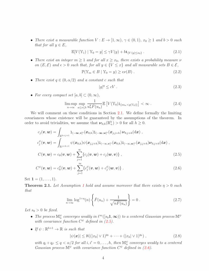
• There exist a measurable function V : E → [1,∞), γ ∈ (0, 1), x0 ≥ 1 and b > 0 suchthat for all y ∈ E,
E[V (Y1) | Y0 = y] ≤ γV (y) + b1V (y)≤x0 . (2.1)
• There exist an integer m ≥ 1 and for all x ≥ x0, there exists a probability measure νon (E, E) and ǫ > 0 such that, for all y ∈ V ≤ x and all measurable sets B ∈ E ,
P(Ym ∈ B | Y0 = y) ≥ ǫν(B) . (2.2)
• There exist q ∈ (0, α/2) and a constant c such that
|g|q ≤ cV . (2.3)
• For every compact set [a, b] ⊂ (0,∞),
lim supn→∞
supa≤s≤b
1
uqnF (un)E[
V (Y0)1sun<g(Y0)
]
<∞ . (2.4)
We will comment on these conditions in Section 2.1. We define formally the limitingcovariances whose existence will be guaranteed by the assumptions of the theorem. Inorder to avoid trivialities, we assume that ν0,h(R
h+) > 0 for all h ≥ 0.
cj(v,w) =
∫
Rh+j+1
1(−∞,v]c(x0,h)1(−∞,w]c(xj,j+h)ν0,j+h(dx) ,
cψj (v,w) =
∫
Rj+h+1
ψ(x0,h)ψ(xj,j+h)1(−∞,v ]c(x0,h)1(−∞,w ]c(xj,j+h)ν0,j+h(dx) ,
C(v,w) = c0(v,w) +
∞∑
j=1
cj(v,w) + cj(w, v) , (2.5)
Cψ(v,w) = cψ0 (v,w) +∞∑
j=1
cψj (v,w) + cψj (w, v) . (2.6)
Set 1 = (1, . . . , 1).
Theorem 2.1. Let Assumption 1 hold and assume moreover that there exists η > 0 suchthat
limn→∞
log1+η(n)
F (un) +1
√
nF (un)
= 0 . (2.7)
Let s0 > 0 be fixed.
• The process Mψn converges weakly in ℓ∞([s01,∞)) to a centered Gaussian process Mψ
with covariance function Cψ defined in (2.5).
• If ψ : Rh+1 → R is such that
|ψ(x)| ≤ ℵ((|x0| ∨ 1)q0 + · · · + (|xh| ∨ 1)qh) , (2.8)
with qi + qi′ ≤ q < α/2 for all i, i′ = 0, . . . , h, then Mψn converges weakly to a centered
Gaussian process Mψ with covariance function Cψ defined in (2.6).
4

2.1 Comments
(C1) Under Assumption 1, it is well known that the chain Yj is irreducible and geomet-rically ergodic. This implies that the chain Yj and the sequence Xj are β-mixingand there exists c > 1 such that βn = O(e−cn); see [Bra05, Theorem 3.7]. This is avery strong requirement, however, it is satisfied by many usual time series models,under standard conditions. See Section 3. Moreover, the geometric drift conditionhas the following consequences.
• Let the stationary distribution of the chain Yj be denoted by π. Then thedrift condition implies that π(V ) <∞.
• It was proved in [MW13] that the geometric drift condition implies the anti-clustering condition (1.3). Under this anti-clustering condition, it is well knownin particular that the extremal index of the sequence Xj is positive. See [BS09,Proposition 4.2]. The geometric drift condition is not necessary for this anti-clustering condition to hold, but when the chain is not geometrically ergodic,nearly any asymptotic behavior of the tail empirical process is possible. SeeSection 3.3.
(C2) Condition (2.4) is an ad-hoc condition which has to be checked for each example. Itis implied by the stronger condition
lim supn→∞
supa≤s≤b
1
uqnF (un)E[
V (Y0)1suqn<V (Y0)
]
<∞ . (2.9)
It holds for instance if Y0 takes values in Rd, is regularly varying with index α and
V (Y0) = 1 + ‖Y0‖q, g(Y0) = Y(1)0 (the first component of Y0).
In order to prove Theorem 2.1, we will use a weighted form of the classical anticluster-ing condition mentioned above. Precisely, for sequences un and rn, we will say thatCondition S(un, rn, ψ) holds if for every pair v,w ∈ (0,∞),
limL→∞
lim supn→∞
1
F (un)
∑
L<|j|≤rn
E [|ψ (X0,h/un)| |ψ (Xj,j+h/un)|1[∞,v]c(X0,h/un)1[−∞,w]c(Xj,j+h/un)]
= 0 . (S(un, rn, ψ))
In Lemma 5.3, we will prove that Assumption 1 and condition (2.8) on the function ψ implythis weighted anti-clustering condition. The proof of this result is rather straightforwardbut lengthy and we postpone it to Section 5. Here, to illustrate it, we prove that S(un, rn, ψ)implies that the series in (2.6) is summable.
Lemma 2.2. Assume that the sequence Xj is regularly varying. Assume moreover that
(2.8) and S(un, rn, ψ) hold, then, for all v,w ∈ (0,∞), the series∑∞
j=1 |cψj (v,w)| is
summable.
5

Proof. Fix positive integers R > L ≥ 1 and set
ψn,j(v) = ψ (Xj,j+h/un) 1[∞,v]c(Xj,j+h/un) .
Then, by regular variation, (2.8) and since 2q < α,
R∑
j=L
|cψj (v,w)| = limn→∞
R∑
j=L
E[ψn,0(v)ψn,j(w)]
F (un).
Fix ǫ > 0. Applying S(un, rn, ψ), we can choose L such that, for every fixed R ≥ L
limn→∞
R∑
j=L
E[ψn,0(v)ψn,j(w)]
F (un)≤ ǫ .
This yields that for every ǫ > 0, for large enough L and all R ≥ L,∑R
j=L |cψj (v,w)| ≤ ǫ
and this precisely means that the series∑∞
j=1 |cψj (v,w)| is summable.
3 Two models and a counterexample
The convergence of the tail empirical process has been considered in the literature undermixing assumptions and additional conditions which have been checked for a few specificmodels such as solutions of stochastic recurrence equations (including GARCH processes)and linear processes. See e.g. [Dre00], [Dre03] and [DM09]. Our main result providesa simple condition for functions of geometrically ergodic Markov chains which includemany usual time series models. In the following two subsections, we will prove that theassumptions of Theorem 2.1 hold (and are easily checked) for two models which have notbeen considered (or not fully investigated) in the earlier literature. In Section 3.3, wewill illustrate on a counterexample the fact that the geomtric drift condition, though notnecessary, cannot be innocuously dispensed with.
3.1 AR(p) with regularly varying innovations
Convergence of the tail empirical processes of exceedances for infinite order moving av-erages has been obtained in the case of finite variance innovation; for infinite varianceinnovations it was proved only in the case of an AR(1) process in [Dre03]. We next showthat Assumption 1 holds for general causal invertible AR(p) models.
Corollary 3.1. Assume that Xj , j ∈ Z is an AR(p) model
Xj = φ1Xj−1 + · · · + φpXj−p + εj , j ≥ 1 ,
that satisfies the following conditions:
• the innovations εj, j ∈ Z are i.i.d. and regularly varying with index α;
6

• the innovations have a density fε not vanishing in a neighbourhood of zero;
• the spectral radius of the matrix
Σ =
φ1 φ2 · · · φp1 0 · · · 0...
.... . .
...1 0 · · · 0
,
is smaller than 1.
• if α ≤ 2, then∑p
i=1 |φi|q < 1 for q = min1, α.
Then Assumption 1 holds.
Proof. The AR(p) process can be embedded into an Rp-valued vector-autoregressive Markovchain
Yj = ΣYj−1 + Zj (3.1)
with
Yj = (Xj , . . . , Xj−p+1)T , Zj = (εj, 0, . . . , 0)T .
Since the spectral radius of Σ is smaller than 1, the stationary solution to (3.1) exists andis given by Yj =
∑∞k=0 Σk
Yj−k. Since the innovation εj is regularly varying, the chainYj is also regularly varying with index α. The AR(p) process is recovered by takingXj = g(Yj) with g(y) = g(y1, . . . , yp) = y1 and Xj , j ∈ Z is also regularly varying.Hence, the first two items of Assumption 1 are fulfilled. Due to the assumption on theinnovations density, the chain is an irreducible and aperiodic T -chain (see e.g. [FT85]).Thus, by [MT09, Theorem 6.0.1], all compact sets are small sets.
We now check the drift condition (2.1). Let λ be the spectral radius of the matrix Σ.Fix ǫ such that γ = λ+ ǫ < 1. Then there exists a norm ‖ · ‖Σ on Rp such that the matrixnorm of Σ with respect to this norm is at most γ, that is
supx∈Rp
‖x‖Σ=1
‖Σx‖Σ ≤ γ .
See [DMS14, Proposition 4.24 and Example 6.35] for more details. Choose such a normand for q < α, set Vq(y) = 1 + ‖y‖qΣ and vq = ‖(1, 0, . . . , 0)‖qΣ. If q ≤ 1, then we will usethe inequality (x+ y)q ≤ xq + yq. If q > 1, then for every η ∈ (0, 1), there exists a constantCq such that for all x, y ≥ 0,
(x+ y)q ≤ (1 + η)xq + Cqyq . (3.2)
7

(Take for instance Cq = 1− (1 + η)−1/(1−q)1−q.) Set cq = Cq = 1 if q ≤ 1 and cq = (1 + η)and Cq as above if q > 1. This yields
E[Vq(Y1) | Y0 = y] ≤ 1 + cq‖Σy‖qΣ + CqvqE[|ε0|q]≤ 1 + cqγ
q‖y‖qΣ + CqvqE[|ε0|q] = λqVq(x) + bq
where λq = cqγq is smaller than 1 if q ≤ 1 or can be made smaller than 1 by choosing an
appropriately small η if q > 1 and bq = 1 − λq + Cq,εvqE[|ε1|q]. Since all compact sets aresmall, this yields (2.1). Furthermore, |g(y)|q ≤ cVq(y) and by regular variation,
limn→∞
1
unF (un)E[
Vq(Y0)1sun<g(Y0)
]
=
∫
xp>s
∫
Rp−1
1 + ‖x‖qΣν1,p(dx) .
Hence, Assumption 1 holds for all q < α. Conditions (2.3) and (2.4) hold, see Com-ment (C2).
3.2 Threshold ARCH
Corollary 3.2. Let ξ ∈ R. Assume that Xj is T-ARCH model
Xj = (b10 + b11X2j−1)
1/2Zj1Xj−1<ξ + (b20 + b21X2j−1)
1/2Zj1Xj−1≥ξ , (3.3)
that satisfies the following conditions:
• bij > 0;
• the innovations Zj, j ∈ Z are i.i.d. such that E[|Zβj |] <∞ for all β > 0;
• the innovations have a density fZ not vanishing in a neighbourhood of zero andbounded;
• the Lyapunov exponent
γ = p log b1/211 + (1 − p) log b
1/221 + E[log(|Z1|)] ,
where p = P(Z1 < 0), is strictly negative;
• (b11 ∨ b21)q/2E[|Z0|q] < 1.
Then Assumption 1 holds.
Proof. Under the stated conditions, the Markov chain Xj is an irreducible and aperiodicT -chain; see [Cli07]. Since the Lyapunov exponent is negative, [Cli07, Theorem 2.2] impliesthat the stationary distribution exists and the chain is geometrically ergodic. The station-ary distribution is regularly varying and the index of regular variation of X1 is obtainedby solving
bα/211 E[|Z1|α1Z1<0] + b
α/221 E[|Z1|α1Z1≥0] = 1 ;
8

see again [Cli07]. To check the drift condition, let q < α. Set V (x) = 1 + |x|q. Using (3.2)we have
E [V (X0) | X0 = x]
= 1 + (b10 + b11x2)q/21x<ξ + (b20 + b21x
2)q/21x≥ξE[|Z0|q]≤ 1 + (1 + η)bq/211 1x<ξ + b
q/221 1x≥ξE[|Z0|q] |x|q +Bq ,
with Bq = Cqbq/210 1x<ξ + bq/220 1x≥ξE[|Z0|q]. Finally, since we have here V (x) = 1 + |x|q,
Condition (2.4) holds by regular variation.
3.3 A Counterexample
The geometric drift condition is not a necessary condition for the conclusions of Theo-rem 2.1 to hold, but when it does not hold, it is easy to build counterexamples of nongeometrically ergodic Markov chains which exhibit a highly non standard behaviour oftheir tail empirical process.
Let Zj , j ∈ Z be a sequence of i.i.d. positive integer valued random variables withregularly varying right tail with index β > 1. Define the Markov chain Xj, j ≥ 0 by thefollowing recursion:
Xj =
Xj−1 − 1 if Xj−1 > 1 ,
Zj if Xj−1 = 1 .
Since β > 1, the chain admits a stationary distribution π on N given by
π(n) =P(Z0 ≥ n)
E[Z0], n ≥ 1 .
To avoid confusion, we will denote the distributions functions of Z0 and X0 (when the initialdistribution is π) by FZ and FX , respectively. The tail FX of the stationary distributionis then regularly varying with index α = β − 1, since it is given by
FX(x) =E[(Z0 − [x])+]
E[Z0]∼ xFZ(x)
βE[Z0]. (3.4)
Assuming for simplicity that P(Z0 = n) > 0 for all n ≥ 1, this chain is irreducible andaperiodic and the state 1 is a recurrent atom. The distribution of the return time τ1 tothe atom 1, when the chains starts from 1 is the distribution of Z0. Hence the chain isnot geometrically ergodic since under the assumption on Z0, E1[κ
τ1 ] = E[κZ0 ] = ∞ forall κ > 1. Moreover, the extremal index of the chain is 0, by an application of [Roo88,Theorem 3.2 and Eq. 4.2].
Let un be a scaling sequence and define the usual univariate tail empirical distributionfunction by
Tn(s) =1
nFX(un)
n∑
j=1
1Xj>uns , (3.5)
9

and Tn(s) = E|Tn(s)] = FX(uns)/FX(un). Let an be a scaling sequence such thatlimn→∞ nP(Z0 > an) = 1.
Proposition 3.3. • If limn→∞ nFZ(un) = 0, then limn→∞ P(Tn(s) 6= 0) = 0.
• If β ∈ (1, 2) and limn→∞ nFZ(un) = ∞, then there exists a β-stable random variable Λ
such that for every s > 0, a−1n nFX(un)Tn(s) − Tn(s) d→ Λ.
• If β > 2, limn→∞ nFZ(un) = ∞ and s0 > 0 then the process s→√
nFZ(un)Tn(s)−Tn(s) converges weakly in ℓ∞([s0,∞)) to a centered Gaussian process G with covari-ance function
C(s, t) =(β + 1)t1−β
β(β − 1)− st−β
β, s < t .
Remark 3.4. • In the standard situation (for example, under the geometric drift condi-tion), a non degenerate limit is expected if nFX(un) → ∞. Since FX(un) ∼ unFZ(un),it may happen simultaneously that nFX(un) → ∞ and nFZ(un) → 0. The appro-priate threshold is determined by the distribution of Z0 and not by the stationarydistribution of the chain.
• In the case 1 < β < 2, a−1n nFX(un) = FX(un)/FX(an) → ∞, thus the tail empiricaldistribution is consistent, but since the limiting distribution of the TEP does notdepend on s, it might be useless for inference.
4 Statistical applications
In statistical applications the presence of the sequence un is not desirable. Let k be anintermediate sequence and let the sequence un be defined by un = F←(1−k/n) where F←
is the left continuous generalized inverse of F . If F is continuous, then k = nF (un). Givena sample X1, . . . , Xn, let Xn:1, . . . , Xn:n be the increasing order statistics of the sample. Instatistical applications, the sequence un is replaced by Xn:n−k, the k+1 largest observationin the sample.
In this section, we will give the asymptotic covariances in terms of the tail processYj, j ∈ Z or spectral tail process Θj, j ∈ Z, introduced by [BS09]. The regularvariation of the time series Xj, j ∈ Z is equivalent to the existence of these processesdefined as follows: for j ≤ k ∈ Z,
P((Yj, . . . , Yk) ∈ ·) = limx→∞
P(x−1(X−j, . . . , Xk) ∈ · | |X0| > x) ,
Θj = Yj/|Y0| .
Then |Y0| is a standard Pareto random variable with tail index α, independent of thesequence Θj, j ∈ Z. The tail process provides in some cases convenient expressionsof the asymptotic limits of the estimates, though in any case, these variances must beestimated.
10

Bias issues. When studying estimators, a bias term appears. In extreme value statis-tics, dealing with the bias means being able to make a suitable choice of the number kof order statistics that are used. Such a choice is always theoretically possible (see condi-tions (4.4), (4.14) and (4.8) below). The practical issue of a data-driven choice of k is notadressed here.
4.1 Convergence of order statistics
Consider the univariate TED and the univariate TEP
Tn = Mn(s,∞, · · · ,∞) =1
nF (un)
n∑
j=1
1Xj>uns , (4.1)
Tn(s) = E[Tn(s)] =F (uns)
F (un), (4.2)
Gn(s) =√
nF (un)Tn(s) − Tn(s) = Mn(s,∞, . . . ,∞) . (4.3)
By Theorem 2.1, Gn converges weakly to the Gaussian process G defined by G(s) =M(s,∞, . . . ,∞). Note that F (uns)/F (un) converges to s−α, uniformly on every interval[s0,∞]. Define
Bn(s0) = sups≥s0
∣
∣
∣
∣
F (uns)
F (un)− s−α
∣
∣
∣
∣
and assume that
limn→∞
√kBn(s0) = 0 . (4.4)
Corollary 4.1. Under the assumptions of Theorem 2.1 and if additionally (4.4) holds then
√k
Xn:n−k
un− 1
d→ α−1G(1) . (4.5)
Moreover, the convergence holds jointly with that of Mψn to Mψ for any function ψ satisfying
the assumption of Theorem 2.1.
The proof is a standard application of Theorem 2.1 and Vervaat’s Lemma and is omitted(see e.g. [Roo09]; [KS11].) The autocovariance function C of the process G is given by (2.5):
C(v, w) = c0(v, w) +
∞∑
j=1
cj(v, w) + cj(w, v) ,
where
cj(v, w) = limn→∞
P(X0 > unv,Xj > unw)
F (un)=
∫
Rj+1
1(v,∞)(x0)1(w,∞)(xj)ν0,j(dx) .
11

In the language of [DM09], the sequence of coefficients cj is the extremogram of Xjrelated to the sets (v,∞), (w,∞). Using the tail process Yj or the spectral tail processΘj, the coefficient cj can be represented as
cj(v, w) = v−αP(Yj > w/v | Y0 > 1) = v−αE[
(Θjv/w)α+ ∧ 1 | Θ0 = 1]
.
This yields
var(G(1)) = C(1, 1) = 1 + 2
∞∑
j=1
P(Yj > 1 | Y0 > 1)
= 1 + 2∞∑
j=1
E[(Θj)α+ ∧ 1 | Θ0 = 1] =
∑
j∈Z
E[(Θj)α+ ∧ 1 | Θ0 = 1] .
In particular, if the sequence Xj is extremally independent, which means that all theexponent measures ν0,j are concentrated on the axes, then Θj = 0 for j 6= 0 and thelimiting distribution in (4.5) is normal with mean zero and variance α−2.
Counterexample, continued. We now investigate the order statistics for the coun-terexample of Section 3.3. Consider the case β > 2 and limn→∞ nFZ(un) = ∞. Anapplication of Vervaat’s Lemma (see the argument in [Roo09] or [KS11]) yields
√
nFZ(un)(
Tn T←n (1) − 1)
d→ −(G T←)(1) ,
where Tn, Tn are defined in (4.1), and T (s) = s−α, whith α = β − 1, the tail index of thestationary distribution. A Taylor expansion yields
Tn T←n (1) − 1 ≈ T ′n(T←n (1))
T←n (1) − T←n (1)
.
Set again un = F←X (1−k/n). Then T←n (1) = Xn:n−k/un, as well as T←n (1) = 1. Under suit-able regularity conditions which ensure that T ′n converges uniformly in the neighbourhoodof 1, we have
√
nFZ(un)
Xn:n−k
un− 1
d→ α−1G(1)
or equivalently,
√
k/un
Xn:n−k
un− 1
d→ α−1G(1) .
The limiting distribution is normal with variance 2α−4(α − 1)−1. If nFZ(un) → 1, thenk ∼ un → ∞ but in that case, for j = o(un), u−1n Xn:n−j converges weakly to one singleFrechet distribution with tail index β.
12

4.2 Hill estimator
The classical Hill estimator of γ = 1/α is defined as
γ =1
k
n∑
j=1
log+
(
Xn:n−j+1
Xn:n−k
)
.
Under the conditions ensuring that Xn:n−k/un →P= 1, the order statistics appearing in thedefinitoin of the estimator are all positive with probability tending to 1, thus the estimatoris well defined.
Corollary 4.2. Under the assumptions of Theorem 2.1 and if moreover (4.4) holds,√k γ − γ converges weakly to a centered Gaussian distribution with variance
α−2
1 + 2
∞∑
j=1
P(Yj > 1 | Y0 > 1)
= α−2
1 + 2
∞∑
j=1
E[(Θj)α+ ∧ 1 | Θ0 = 1]
. (4.6)
This result provides the asymptotic normality of the Hill estimator for all irreducibleMarkov chains that satisfy the geometric drift condition. The proof is again a standardapplication of Theorem 2.1 and is omitted. The expression for the limiting variance isjustified in Section 5.5. In the case of an extremally independent time series where Θj = 0for j 6= 0, the variance is simply α−2 as in the case of an i.i.d. sequence.
4.3 Estimation of the extremal index
Set Ah = x0 ∨ · · · ∨ xh > 1 and consider
ν0,h(Ah) = limx→∞
P(X0 ∨ · · · ∨Xh > x)
F (x).
By conditioning on the last index j ≤ h such that Xj > x, we can express this limit interms of the spectral tail process:
ν0,h(Ah) = 1 +h−1∑
j=1
P(∨ji=1Yi ≤ 1 | Y0 > 1) .
It has been proved in [BS09] that the anticlustering condition (1.3) implies that the right-tail extremal index θ+ of the sequence Xi is positive, and moreover, θ+ = P(maxj≥1 Yj ≤1 | Y0 > 1). Since the drift condition (2.1) implies the anticlustering condition, we obtain
θ+ = limh→∞
ν0,h(Ah)
h∈ [0,∞) .
Set θ+(h) = h−1ν0,h(Ah). Then a natural estimator of θ+(h) can be defined by
θn(h) =1
hk
n−h∑
j=1
1Xj∨···∨Xj+h>Xn:n−k = h−1Mn(u−1n Xn:n−k1) .
13

This yields, applying the homogeneity of the measure ν0,h,
√kθn(h) − θ+(h) = h−1Mn,h(u
−1n Xn:n−k1) (4.7a)
+n− h
nh
√kMn(u−1n Xn:n−k1) − ν0,h(Xn:n−kAh/un) (4.7b)
+n− h
nh
√k(Xn:n−k/un)−α − 1ν0,h(Ah) +
h
nθ+(h) . (4.7c)
In order to prove the convergence, we need an additional condition to deal with the biasterm in (4.7b). For s > 0, define
Bn(h, s0) = sups≥s0
∣
∣
∣
∣
P(X0 ∨ · · · ∨Xh > uns)
F (un)− s−αν0,h(Ah)
∣
∣
∣
∣
.
Since the function s→ P(X0 ∨ · · · ∨Xh > uns)/F (un) is monotone and its limit is contin-uous, the convergence is also uniform on [s0,∞] for every s0 > 0. Therefore, we assumethat the intermediate sequence k is chosen in such a way that
limn→∞
√kBn(h, s0) = 0 , (4.8)
for a fixed s0 ∈ (0, 1).
Corollary 4.3. Under the assumptions of Theorem 2.1 and if moreover (4.4) and (4.8)hold,
√k(θn(h) − θ+(h)) converges weakly to h−1Mh(1) − θ+(h)G(1).
Proof. Since the present assumptions subsume those of Corollary 4.1, Xn:n−k/unp→ 1 and√
k(Xn:n−k/un)−α−1) → −G(1). Moreover, Theorem 2.1 implies that Mn(u−1n Xn:n−k1)d→
M(1), and the convergence holds jointly. Condition (4.8) implies that the bias termin (4.7b) is asymptotically vanishing. The result follows.
Note that we are not estimating the extremal index, but only the quantity θ+(h) whichconverges to it as h → ∞. Therefore, it is not devoid of interest; and for practicalpurposes, h is necessarily finite. Moreover, we can improve on this approximation. SinceP(Y1∨· · ·∨Yh ≤ 1 | Y0 > 1), h ≥ 1 is a decreasing sequence with limit θ+, for each h ≥ 1,P(Y1 ∨ · · · ∨ Yh ≤ 1 | Y0 > 1) is closer to its limit θ+ (as h → ∞) than its Cesaro mean.Therefore, it is probably a better idea to estimate this quantity rather than θ+(h). This isindeed the case for certain models, as noted by [Hsi93, Example C]. Since by definition
θ+(h) = hθ+(h) − (h− 1)θ+(h− 1) = limx→∞
P(X0 ≤ x, . . . , Xh−1 ≤ x,Xh > x)
F (x),
an estimator of θ+(h) is defined by
θn(h) =1
k
n∑
i=1
1Xi∨···∨Xi+h−1≤Xn:n−k,Xi+h>Xn:n−k, .
14

This estimator was considered by [Hsi93] under ad-hoc summabiliy assumption for thecovariances of the indicators in the definition of the estimator which is implied by theanticlustering condition, hence by the drift condition. It can be similarly proved that undersuitable bias conditions on k,
√k(θn(h) − θ+(h)) converges weakly to a centered Gaussian
distribution which can be expressed as Mh(1, . . . , 1,∞)−hθ+(h)− (h−1)θ+(h−1)G(1).
4.4 Estimation of the cluster index
In a very similar way, with maxima replaced by sums, we can obtain the limiting distribu-tion for an estimator of the cluster index. For Ah = x0 + · · · + xh > 1 we consider
b+(h) =1
hlimn→∞
P(X0 + · · · +Xh > x)
F (x)=
1
hν0,h(Ah) .
It is shown in [MW14] that the drift condition (2.1) implies that
b+ = limh→∞
b+(h) ∈ [0,∞) .
Define
b+(h) =1
kh
n−h∑
j=1
1Xj+···+Xj+h>Xn:n−k .
In order to prove the convergence, we need an additional condition. For s > 0, define
Dn(h, s0) = sups≥s0
∣
∣
∣
∣
P(X0 + · · · +Xh > uns)
F (un)− s−αν0,h(Ah)
∣
∣
∣
∣
.
We assume that the intermediate sequence k is chosen in such a way that
limn→∞
√kDn(h, s0) = 0 , (4.9)
for a fixed s0 ∈ (0, 1).
Corollary 4.4. Under the assumptions of Theorem 2.1 and if moreover (4.4) and (4.9)hold,
√k(b+(h) − b+(h)) converges weakly to a zero mean Gaussian random variable.
The proof is similar to the proof of Corollary 4.3 and is omitted.
4.5 Conditional tail expectation
If the tail index of the time series Xj is α > 1, then the following limit exists:
limu→∞
1
uE[Xh | X0 > ux] =
∫ ∞
x0=1
∫
Rh
xh ν0,h(dx) = CTE(h) . (4.10)
15

The quantity above is the conditional tail expectation and when h = 0 it is being used(under the name expected shortfall) as a risk measure, a coherent alternative to the popularvalue-at-risk. In the case of bivariate i.i.d. vectors with the same distribution as (X, Y ),statistical procedures for estimating E[Y | X > QX(1 − p)] when p → 0, where QX(p) =F←X (1 − p), were developed in [CEdHZ15]. The limit (4.10) yields the approximation
E[Xh | X0 > F←(1 − p)] ∼ F←(1 − p)CTE(h) .
If p ≈ 1/n, this becomes an extrapolation problem, related to the estimation of extremequantiles. if αn is an estimator of the right tail index α of the marginal distribution, thenan estimator of the quantile of order p is given by
Xn:n−k
(
k
np
)1/αn
.
The rationale for this estimator is the approximation F←(1 − p) ∼ F←(1 − k/n)(k/np)1/α
and the convergence Xn:n−k/F←(1 − k/n)
p→ 1 established above. A simple estimator ofCTE(h) is given by
Cn(h) =1
kXnn:n−k
n∑
j=1
Xj+h1Xj>Xn:n−k
This yields an estimator of Eh(p) = E[Xh | X0 > F←(1 − p)]:
En = Xn:n−k
(
k
np
)1/αn
Cn(h) =
(
k
np
)1/αn 1
k
n∑
j=1
Xj+h1Xj>Xn:n−k .
We will focus here on the asymptotic distribution of Cn(h)−CTE(h) suitably normalized.
The application to the limiting distribution of√k
En/Eh(p) − 1
when p = pn ≈ n−1 is
straightforward, given additional ad-hoc bias assumptions. Define
Tn,h(s) =1
kun
n∑
j=1
Xj+h1Xi>uns , (4.11)
Tn,h(s) = E[Tn,h(s)] =1
unF (un)E[
Xh1X0>uns
]
. (4.12)
Regular variation and α > 1 imply
Th(s) = limn→∞
Tn,h(s) = s−α∫ ∞
x0=1
∫
Rh
xhν0,h(dx0,h) = s−αCTE(h) . (4.13)
We shall assume that
limn→∞
√k sups≥s0
|Tn,h(s) − Th(s)| = 0 . (4.14)
16

Then
√k
Cn(h) − CTE(h)
=un
Xn:n−k
√k
Tn,h(Xn:n−k/un) − Tn,h(Xn:n−k/un)
(4.15a)
+un
Xn:n−k
√k
Tn,h(Xn:n−k/un) − (Xn:n−k/un)−αCTE(h)
(4.15b)
+√k
(Xn:n−k/un)−α−1 − 1
CTE(h) . (4.15c)
If (4.4) holds then we can apply Corollary 4.1. In particular, Xn:n−k/unp→ 1. As usual,
the term in (4.15b) is a bias term which vanishes thanks to (4.14). If α > 2, applying The-orem 2.1, the term in (4.15a) has a Gaussian limit which can be expressed as M
ψh (1) with
ψ(x) = x. The last terms converges to −α−1(α + 1)G(1).
Corollary 4.5. Under the assumptions of Theorem 2.1 and if moreover (4.4) and (4.14)
hold,√k
Cn − CTE(h)
converges weakly to Mψh (1) − α−1(α+ 1)CTE(h)G(1).
5 Proofs
5.1 Proof of Condition S(un, rn, ψ)
As mentioned in Section 2.1, the main ingredient of the proof is Condition S(un, rn, ψ). Inorder to prove that it is implied by the drift condition (2.1), we recall some consequencesof the geometric drift condition. Under condition (2.2), the chain Yj can be embeddedinto an extended Markov chain (Yj, Bj) such that the latter chain possesses an atom A,that is P (s, ·) = P (t, ·) for every s, t ∈ A, where P is the transition kernel of the extendedchain. This existence is due to the Nummelin splitting technique (see [MT09, Chapter 5]).Denote by EA the expectation conditionally to (Y0, B0) ∈ A and let τA be the first returntime to A of the chain (Yj, Bj), j ≥ 0. Note that τA is a stopping time with restect tothe extended chain, but not with respect to the chain Yj. We assume that the extendedchain is defined on the orginal probability space (Ω,F ,P) and that the extended chain isstationary under P. Then, there exist κ > 1 and a constant ℵ such that for all y ∈ E,
E
[
τA∑
j=1
κj|Xj|q | Y0 = y
]
≤ cE
[
τA∑
j=1
κjV (Yj) | Y0 = y
]
≤ ℵV (y) . (5.1)
By Jensen’s inequality, this implies that for all q1 ≤ q, there exists κ1 ∈ (1, κ) such that
E
[
τA∑
j=1
κj1|Xj |q1 | Y0 = y
]
≤ ℵV q1/q(y) . (5.2)
Moreover, Kac’s formula [MT09, Theorem 15.0.1] gives an expression of the stationarydistribution in terms of the return time to A. For every bounded measurable function f ,
17

it holds that
E[f(Y0)] =1
EA[τA]EA
[
τA−1∑
i=0
f(Yi)
]
. (5.3)
Since V ≥ 1, the inequality (5.1) integrated with respect to the stationary distributionimplies that E[κτA ] <∞. For q ≥ 0 and 0 < s < t ≤ ∞ define
Qn(s) =1
uqnF (un)E[
V (Y0)1sun<X0
]
,
and Qn(s, t) = Qn(s) −Qn(t).
Lemma 5.1. Let Assumption 1 holds. For every s0 > 0, there exists a constant ℵ suchthat for q1 + q2 ≤ q, L > h and t > s ≥ s0,
1
F (un)E
[
τA∑
j=L
1sun<X0≤tun|Xh/un|q1|Xj/un|q2]
≤ ℵκ−LQq2/qn (s, t) +Qn(s, t) . (5.4)
Proof. Let the left hand side of (5.4) be denoted by Sn(s, t). Splitting the expectationbetween |Xh| ≤ un and |Xh| > un yields
Sn(s, t) ≤ 1
F (un)E
[
τA∑
j=L
1sun<X0≤tun|Xj/un|q2]
+1
F (un)E
[
τA∑
j=L
1sun<X0≤tun1un<|Xh||Xh/un|q1|Xj/un|q2]
= Sn,1(s, t) + Sn,2(s, t) .
Applying the bound (5.2) and Jensen’s inequality (since q2 ≤ q), we obtain
Sn,1(s, t) ≤1
uq2n F (un)E[
V q2/q(Y0)1sun<X0≤tun
]
≤ ℵκ−LQq2/qn (s, t) .
18

By the Markov property and the bound (5.2) (and noting that q2 ≤ q − q1), we obtain
Sn,2(s, t) =1
F (un)E
[
τA∑
j=L
1sun<X0≤tun1un<|Xh||Xh/un|q1|Xj/un|q2]
=1
F (un)E
[1sun<X0≤tun1un<|Xh||Xh/un|q1E[
τA∑
j=L
|Xj/un|q2 | Yh
]]
=κ−L2
F (un)E
[1sun<X0≤tun1un<|Xh||Xh/un|q1E[
τA∑
j=L
κj2|Xj/un|q2 | Yh
]]
≤ ℵ κ−L2
uq2n F (un)E[1sun<X0≤tun1un<|Xh||Xh/un|q1V q2/q(Yh)
]
≤ ℵ κ−L2
uq2n F (un)E[1sun<X0≤tun1un<|Xh||Xh/un|q−q2V q2/q(Yh)
]
≤ ℵ κ−L2
uqnF (un)E[1sun<X0≤tunV (Yh)
]
.
Iterating the drift condition (2.1) (and since V ≥ 1), we obtain that
E[V (Yh) | Y0 = y] ≤ γhV (y) +b
1 − γ≤ ℵV (y) .
This yields
Sn,2(s, t) ≤ ℵ κ−L2
uqnF (un)E[1sun<X0≤tunV (Y0)
]
≤ ℵκ−LQn(s, t) .
Lemma 5.2. If Assumption 1 holds, rnF (un) = o(1), and q1 + q2 ≤ q < α, then
1
F (un)E
[1τA>h rn∑
j=τA+1
1sun<X0≤tun1sun<Xj≤tun|Xh/un|q1|Xj/un|q2]
= o(1) . (5.5)
Proof. Let the left handside of (5.5) be denoted Rn. Then, by the strong Markov property,
Rn ≤ 1
F (un)E
[1sun<X0|Xh/un|q1E[
rn∑
j=τA+1
1sun<Xj|Xj/un|q2 | FτA
]]
≤ 1
F (un)E
[1sun<X0|Xh/un|q11τA>hE[ rn+τA∑
j=τA+1
1sun<Xj|Xj/un|q2 | FτA
]]
≤ 1
F (un)E[1sun<X0|Xh/un|q1
]
EA
[
rn∑
j=1
1sun<Xj|Xj/un|q2]
.
19

By classical regenerative arguments, Kac’s formula (5.3) and regular variation, we obtainas n→ ∞,
EA
[
rn∑
j=1
1sun<Xj|Xj/un|q2]
∼ rnEA[τA]
EA
[
τA∑
j=1
1sun<Xj|Xj/un|q2]
≤ rnF (un)E[1X0>uns0|X0/un|q2]
F (un)= O(rnF (un)) .
This yields, applying again the drift condition, Condition (2.4) and Jensen’s inequailty,
Rn ≤ O(rn)E[1X0>uns0|Xh/un|q1
]
= O(rnF (un))E[
V q1/q(Y0) | X0 > uns0]
uq1n
= O(rnF (un))
(
E [V (Y0) | X0 > uns0]
uqn
)q1/q
= o(1) .
Lemma 5.3. Let Assumption 1 and (2.8) hold and rnF (un) = o(1). Then Condition S(un, rn, ψ)holds.
Proof. By assumption (2.8), and for every v,w ∈ (0,∞), there exists ǫ > 0 such that forj ≥ h,
0 ≤ 1[∞,v]c(X0,h/un)1[∞,w]c(Xj,j+h/un)|ψ(X0,h/un)||ψ(Xj,j+h/un)|
≤ ℵu−qi2−qi4n
h∑
i1,i2,i3,i4=0
1ǫun<Xi1|Xi2 |qi21ǫun<Xj+i3
|Xj+i4|qi4 . (5.6)
For all i, i′, we can write1ǫun<Xi|Xi′/un|q ≤ 1ǫun<Xi|Xi/un|q + 1un ǫ<Xi′|Xi′/un|q .
Thus, we can restrict the sum in (5.6) to the set of indices (i1, i2, i3, i4) such that i1 = i2and i3 = i4 and since h is fixed, there is no loss of generality in restricting further to thecases i1 = i2 = i3 = i4 = 0. For an integer L > 0, splitting the sum at τA and applyingLemmas 5.1 and 5.2, we obtain, with q1 + q2 ≤ q,
1
F (un)E
[
rn∑
j=L
1sun<X01sun<Xj|X0/un|q1|Xj/un|q2]
≤ 1
F (un)E
[
τA∑
j=L
1sun<X01sun<Xj|X0/un|q1|Xj/un|q2]
+1
F (un)E
[
rn∑
j=τA+1
1sun<X01sun<Xj|X0/un|q1|Xj/un|q2]
≤ ℵκ−LQq2/qn (s) +Qn(s) + o(1) .
20
This proves that S(un, rn, ψ) holds since Qn is asymptotically locally uniformly boundedby (2.4).
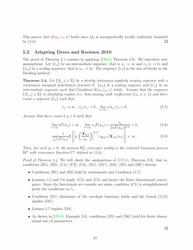
5.2 Adapting Drees and Rootzen 2010
The proof of Theorem 2.1 consists in applying [DR10, Theorem 2.8]. We introduce newassumptions. Let rn be an intermediate sequence, that is rn → ∞ and rn/n → 0, andun be a scaling sequence, that is un → ∞. The sequence rn is the size of blocks in theblocking method.
Theorem 5.4. Let Xj, j ∈ Z be a strictly stationary regularly varying sequence with acontinuous marginal distribution function F , un be a scaling sequence and rn be anintermediate sequence such that Condition S(un, rn, ψ) holds. Assume that the sequenceXj, j ∈ Z is absolutely regular (i.e. beta-mixing) with coefficients βn, n ≥ 1 and thereexists a sequence ℓn such that
ℓn → ∞ , ℓn/rn → 0 , limn→∞
nβℓn/rn = 0 . (5.7)
Assume that there exists δ, η > 0 such that
limn→∞
nF (un) = ∞ , limn→∞
rnF (un) =rn
nF (un)δ/2 = 0 , (5.8)
supn≥1
1
F (un)E
[
∣
∣
∣
∣
ψ
(
X0,h
un
)∣
∣
∣
∣
2+δ 1[0,v ]c(X0,h/un)
]
<∞ . (5.9)
Then, for each s0 > 0, the process Mψn converges weakly to the centered Gaussian process
Mψ with covariance function Cψ defined in (2.6).
Proof of Theorem 5.4. We will check the assumptions of [DR10, Theorem 2.8], that is,conditions (B1), (B2), (C1), (C2), (C3), (D1), (D2’), (D3), (D5) and (D6’) therein.
• Conditions (B1) and (B2) hold by stationarity and Condition (5.7).
• Lemmas 5.5 and 5.6 imply (C2) and (C3) and hence the finite dimensional conver-gence. Since the functionals we consider are sums, condition (C1) is straightforwardgiven the conditions on ln.
• Condition (D1) (finiteness of the envelope function) holds and the bound (5.12)implies (D2’).
• Lemma 5.7 implies (D3).
• As shown in [DR10, Example 3.8], conditions (D5) and (D6’) hold for finite dimen-sional sets of parameters.
21

We now state and prove the needed lemmas. For conciseness, set, for v,∈ (0,∞),
ψn,j(v) = ψ(Xj,j+h/un)1(−∞,v]c(Xj,j+h/un) , Sn(v) =
rn∑
j=1
ψn,j(v) .
Lemma 5.5. If Conditions S(un, rn, ψ) and (5.9) hold, then the series∑∞
j=1 |cψj (v,w)| is
summable. If moreover Condition (5.8) holds, then, for all v,w ∈ (0,∞),
limn→∞
cov(Sn(v), Sn(w))
rnF (un)= Cψ(v,w) .
Proof. The first statement was already proved in Lemma 2.2. For a fixed integer L, wehave
cov(Sn(v), Sn(w))
rnF (un)=
∑
1≤j,j′≤rn
E[ψn,j(v)ψn,j′(w)]
rnF (un)+
∑
1≤j,j′≤rn
E[ψn,j(v)]E[ψn,j′(w)]
rnF (un).
The terms with products of expectations are negligible since by regular variation the nor-malization which makes these terms convergent is F 2(un). Thus we only deal with themain terms. Fix an integer L > h. Then, by stationarity,
∑
1≤j,j′≤rn
E[ψn,j(v)ψn,j′(w)]
rnF (un)=
E[ψn,0(v)ψn,0(w)]
F (un)
+
L∑
j=1
(1 − j/rn)E[ψn,0(v)ψn,j(w)] + E[ψn,j(v)ψn,0(w)]
F (un)
+rn∑
j=L+1
(1 − |j|/rn)E[ψn,0(v)ψn,j(w)] + E[ψn,0(v)ψn,j(w)]
F (un).
By Condition S(un, rn, ψ), for every ǫ > 0, we can choose L such that
lim supn→∞
rn∑
j=L+1
E[|ψn,0(v)ψn,j(w)|] + E[|ψn,0(v)ψn,j(w)|]F (un)
≤ ǫ .
By regular variation and (5.9), we have
limn→∞
(
E[ψn,0(v)ψn,0(w)]
F (un)+
L∑
j=1
(1 − j/rn)E[ψn,j(v)ψn,j′(w)]
F (un)
)
= cψ0 (v,w) +
L∑
j=1
cψj (v,w) + cψj (w, v) .
22

Since we have proved that the series∑∞
j=1 |cψj (v,w)| is convergent, choosing L large enough
yields
lim supn→∞
∣
∣
∣
∣
∣
∑
1≤j,j′≤rn
E[ψn,j(v)ψn,j′(w)]
rnF (un)− Cψ(v,w)
∣
∣
∣
∣
∣
≤ ǫ .
Since ǫ is arbitrary, this concludes the proof.
Lemma 5.6. If Conditions S(un, rn, ψ) (5.8) and (5.9) hold then for all ǫ > 0 and allv ∈ (,∞]h+1,
limn→0
1
rnF (un)E
[
S2n(v)1
|Sn (v)|>ǫ√nF (un)
]
= 0 .
Proof. By monotonicity, the second statement is equivalent to the first one with v = Write
Zn(v, ǫ) =1
rnF (un)E
[
S2n(v)1
|Sn (v)|>ǫ√nF (un)
]
=1
rnF (un)E
[
rn∑
j=1
ψ2n,j(v)1
|Sn (v)|>ǫ√nF (un)
]
+2
rnF (un)
rn∑
i=1
rn∑
j=i+1
E
[
ψn,i(v)ψn,j(v)1|Sn (v)|>ǫ
√nF (un)
]
= Rn +R∗n .
Let δ ∈ (0, 1) be as in (5.8). Using the elementary bound1|Sn (v)|>ǫ
√nF (un)
≤ 1
(ǫ√
nF (un))δ
rn∑
i=1
ψδn,i(v) , (5.11)
we obtain
Rn ≤ 1
rnF (un)ǫ√
nF (un)δE
rn∑
j=1
rn∑
i=1
[
ψ2n,j(v)ψδn,i(v)
]
.
Using Holder’s inequality with p = (2 + δ)/2 and q = (2 + δ)/δ yields
Rn ≤ rn(
ǫ√
nF (un))δ
1
F (un)E[
ψ2+δn,0 (v)
]
.
This bound, (5.8) and (5.9) prove that lim supn→∞Rn = 0. Splitting the sum in j in R∗n
23

at i + L where L is an arbitrary integer, and using (5.11) we obtain
R∗n ≤ 2
rnF (un)
rn∑
i=1
i+L∑
j=i+1
E
[
ψn,i(v)ψn,j(v)1|Sn (v)|≥ǫ
√nF (un)
]
+2
F (un)
rn∑
j=L
E [ψn,0(v)ψn,j(v)]
≤ 2
rnF (un)
1
(ǫ√
nF (un))δ
rn∑
i=1
i+L∑
j=i+1
rn∑
k=1
E[
ψn,i(v)ψn,j(v)ψδn,k(v)]
+2
F (un)
rn∑
j=L
E [ψn,0(v)ψn,j(v)] = R∗n,1(L) +R∗n,2(L) .
Fix η > 0. By Condition S(un, rn, ψ) we can choose L such that lim supn→∞R∗n,2(L) ≤ η.
Then, by Holder’s inequality
lim supn→∞
R∗n,1(L) ≤ lim supn→∞
Lrn
(
ǫ√
nF (un))δ
1
F (un)E[
ψ2+δn,0 (v)
]
= 0 .
Altogether, we have proved that lim supn→∞Zn(v, ǫ) ≤ η for every η > 0. This concludesthe proof.
Fix s0 > 0 and set S = [s01,∞] (with 1 = (1, . . . , 1)) and
S∗n = supv∈S
rn∑
i=1
ψn,i(v) =rn∑
i=1
ψn,i(s01) .
Thus Lemma 5.6 implies that
limn→0
1
rnF (un)E
[
(S∗n)21S∗
n>ǫ√nF (un)
]
= 0 . (5.12)
Define now
ρ(v,w) =1
F (un)
∫
Rh+1
ψ2(x)|1(−∞,v]c(x) − 1(−∞,v]c(x)| ν0,h(dx)
Then ρ is a metric on [0,∞] \ 0 and
ρ(v,w) = limn→∞
1
F (un)E[ψ2(X0,h/un)|1(−∞,v]c(X0,h/un) − 1(−∞,v]c(X0,h/un))|] ,
for all v,w ∈ [0,∞) \ 0.
Lemma 5.7. If Conditions S(un, rn, ψ) and (5.9) hold then, for s0 > 0,
limǫ→0
lim supn→∞
supv,w∈S
ρ(v,w)≤ǫ
1
rnF (un)E[(
Sn(v) − Sn(w))2)]
= 0 .
24
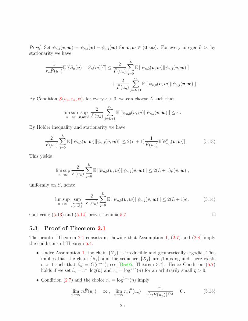
Proof. Set ψn,j(v,w) = ψn,j(v) − ψn,j(w) for v,w ∈ (0,∞). For every integer L >, bystationarity we have
1
rnF (un)E[Sn(v) − Sn(w)2] ≤ 2
F (un)
L∑
j=0
E [|ψn,0(v,w)||ψn,j(v,w)|]
+2
F (un)
rn∑
j=L+1
E [|ψn,0(v,w)||ψn,j(v,w)|] .
By Condition S(un, rn, ψ), for every ǫ > 0, we can choose L such that
lim supn→∞
supv,w∈S
2
F (un)
rn∑
j=L+1
E [|ψn,0(v,w)||ψn,j(v,w)|] ≤ ǫ .
By Holder inequality and stationarity we have
2
F (un)
L∑
j=0
E [|ψn,0(v,w)||ψn,j(v,w)|] ≤ 2(L+ 1)1
F (un)E[ψ2
n,0(v,w)] . (5.13)
This yields
lim supn→∞
2
F (un)
L∑
j=0
E [|ψn,0(v,w)||ψn,j(v,w)|] ≤ 2(L+ 1)ρ(v,w) ,
uniformly on S, hence
lim supn→∞
supv,w∈S
ρ(v,w)≤ǫ
2
F (un)
L∑
j=0
E [|ψn,0(v,w)||ψn,j(v,w)|] ≤ 2(L+ 1)ǫ . (5.14)
Gathering (5.13) and (5.14) proves Lemma 5.7.
5.3 Proof of Theorem 2.1
The proof of Theorem 2.1 consists in showing that Assumption 1, (2.7) and (2.8) implythe conditions of Theorem 5.4.
• Under Assumption 1, the chain Yj is irreducible and geometrically ergodic. Thisimplies that the chain Yj and the sequence Xj are β-mixing and there existsc > 1 such that βn = O(e−cn); see [Bra05, Theorem 3.7]. Hence Condition (5.7)holds if we set ln = c−1 log(n) and rn = log1+η(n) for an arbitrarily small η > 0.
• Condition (2.7) and the choice rn = log1+η(n) imply
limn→∞
nF (un) = ∞ , limn→∞
rnF (un) =rn
nF (un)δ/2 = 0 . (5.15)
25

• Lemma 5.3 shows that Assumption 1, (2.8) and (5.15) imply Condition S(un, rn, ψ)L
• Condition (5.9) follows from regular variation and (2.8). Indeed, for v ∈ [0,∞)\0,we have
lim supn→∞
1
F (un)E
[
∣
∣
∣
∣
ψ
(
X0,h
un
)∣
∣
∣
∣
2+δ 1(−∞,v]c(X0,h)
]
≤ lim supn→∞
∑
0≤i,i′≤h
E[|Xi/un|qi(2+δ)1Xi′>unǫ]
=∑
0≤i,i′≤h
∫
Rh+1
|x|qi(2+δ)1xi′>ǫ ν0,h(dx) .
All these integrals are finite since by assumption, qi(2 + δ) < α for δ small enough.
5.4 Proof of Proposition 3.3
Let Nn be the number of returns to the state 1 before time n, that is
Nn =n∑
j=0
1Xj=1 .
Set also T−1 = −∞, T0 = X0 and Tn = X0 − 1 + Z1 + · · · + Zn for n ≥ 1. Then, Nn isthe counting proess associated to the delayed renewal process Tn. That is, for n, k ≥ 0,
Nn = k ⇔ Tk−1 ≤ n < Tk ,
Since E[Z0] < ∞, setting λ = 1/E[Z0], we have Nn/n → λ a.s. With this notation, wehave, for every s > 0,
n∑
j=0
1Xj>uns = (X0 − [uns])+ +Nn∑
j=1
(Zj − [uns])+ + ζn , (5.16)
where ζn = (n− TNn) ∧ (ZNn − [uns])+ − (Zj − [uns])+ is a correcting term accounting forthe possibly incomplete last portion of the path. Since ζn = OP (1), it does not play anyrole in the asymptotics.
• Consider the case limn→∞ nFZ(un) = 0. Then, for an integer m > λ,
P
(
Nn∑
j=1
(Zj − [uns])+ 6= 0
)
≤ P(Nn > mn) + P
(
mn∑
j=1
(Zj − [uns])+ 6= 0
)
≤ P(Nn > mn) + P(∃j ∈ 1, . . . , mn, Zj > [uns])
≤ P(Nn > mn) +mnFZ([uns]) → 0 .
26

Furthermore,
P ((X0 − [uns])+ 6= 0) = FX([uns]) → 0 .
This proves our first claim.
We proceed with the case limn→∞ nFZ(un) = ∞. Using (3.4) and (5.16) we have
n∑
j=0
1Xj>uns − P(X0 > uns) =
Nn∑
j=1
(Zj − [uns])+ − E[(Z0 − [uns])+]
+ (X0 − [uns])+ + Nn − λn)E[(Z0 − [uns])+] . (5.17)
• Consider the case nFZ(un) → ∞ and β ∈ (1, 2). Since limn→∞ E[(Z0 − [uns])+] = 0,we obtain, for every s > 0,
a−1n
n∑
j=0
1Xj>uns − P(X0 > uns)
= a−1n
Nn∑
j=1
Zj − E[Z0] + a−1n
Nn∑
j=1
Zj ∧ [uns] − E[Z0 ∧ [uns]] + oP (1) .
By regular variation of FZ , we obtain
var
(
n∑
j=1
Zj ∧ [uns] − E[(Z0 ∧ [uns])])
= O(u2nnFZ(un)) .
The regular variation of F and the conditions nFZ(un) → ∞ and nFZ(an) → 1 imply
that un/an → 0. Define h(x) = x√
FZ(x). The function h is regularly varying atinfinity with index 1 − β/2 > 0 and thus
limn→∞
un√
nFZ(un)
an= lim
n→∞
un√
FZ(un)
an√
FZ(an)= lim
n→∞
h(un)
h(an)= 0 .
This yields
a−1n
n∑
j=0
1Xj>uns − P(X0 > uns) = a−1n
Nn∑
j=1
Zj − E[Z0] + oP (1) ,
where the oP (1) term is locally uniform with respect to s > 0. Since the distributionof Z0 is in the domain of attraction of the β-stable law and the sequence Zj is i.i.d.,a−1n (T[ns − λ−1s), s > 0 ⇒ Λ, where Λ is a mean zero, totally skewed to the rightβ-stable Levy process, and the convergence holds with respect to the J1 topology on
27

compact sets of (0,∞). Since limn→∞Nn/n = λ a.s., and since a Levy process isstochastically continuous, this yields, by [Whi02, Proposition 13.2.1],
a−1n
Nn∑
j=1
Zj − E[Z0] d→ Λ(λ)
This proves the second claim.
• Consider now the case β > 2. In that case, Vervaat’s Lemma implies that (Nn −λn)/
√n converges weakly to a gaussian distribution. Thus, (5.17) combined with
E[(Z0 − [uns])+] = O(unFZ(un)), yields
(Nn − λn)E[(Z0 − [uns])+] = OP (unFZ(un)√n) .
Next, we apply the Lindeberg central limit theorem for triangular arrays of indepen-dent random variables to prove that
1
un√
nFZ(un)
n∑
j=1
(Zj − [uns])+ − E[(Z0 − [uns])+] d→ N
(
0,2s1−α
α(α− 1)
)
.
By regular variation of FZ , we have, for all δ ∈ [2, β),
E[(Z0 − uns)δ+] ∼ Cδu
δnFZ(un)sδ−β ,
with Cδ = δ∫∞
1(z − 1)δ−1z−βdz. Set
Yn,j(s) =1
un√
nFZ(un)(Zj − [uns])+ − E[(Z0 − [uns])+] .
The previous computations yield, for δ ∈ (2, β) and s > 0,
limn→∞
nvar(Yn,1(s)) =2s2−β
(β − 1)(β − 2),
nE[|Yn,1|δ] = O
(
nuδnFZ(un)
uδnnFZ(un)δ/2)
= O(
nFZ(un)1−δ/2)
= o(1) .
We conclude that the Lindeberg central limit theorem holds. Convergence of the finitedimensional distribution is done along the same lines and tightness with respect tothe J1 topology on (0,∞) is proved by applying [Bil99, Theorem 13.5].
5.5 Variance of the Hill estimator
Let the processes W and B be defined on [0, 1] by W(s) = G(s−1/α) and B(s) = W(s) −sW(1). Then, the limiting distribution of the Hill estimator is that of the random vari-able α−1Z, with
Z =
∫ 1
0
B(s)ds
s.
28

In the case of extremal independence B is the standard Brownian bridge and var(Z) = 1.In the general case, let γ denote the autocovariance function of W, i.e.
γ(s, t) = s ∧ t+
∞∑
j=1
E[
(sΘαj ) ∧ t+ (tΘα
j ) ∧ s | Θ0 = 1]
.
This yields γ(1, 1) = 1 + 2∑∞
j=1E[Θαj ∧ 1 | Θ0 = 1] and
var(Z) =
∫ 1
0
∫ 1
0
γ(s, t) − sγ(t, 1) − tγ(s, 1) + stγ(1, 1)
stdsdt
= γ(1, 1) +
∫ 1
0
∫ 1
0
γ(s, t)
stdsdt− 2
∫ 1
0
γ(s, 1)
sds .
Note now that γ(s, t) = γ(t, s) and γ(s, t) = sγ(1, t/s), so that
∫ 1
0
∫ 1
0
γ(s, t)
stdsdt = 2
∫ 1
0
∫ t
0
γ(s, t)
stdsdt = 2
∫ 1
0
∫ t
0
γ(s/t, 1)
sdsdt
= 2
∫ 1
0
∫ 1
0
γ(u, 1)
ududt = 2
∫ 1
0
γ(u, 1)
udu .
This shows that var(Z) = γ(1, 1) = 1 + 2∑∞
j=1 E[Θαj ∧ 1 | Θ0 = 1], which proves (4.6).
Acknowledgements The research of Rafal Kulik was supported by the NSERC grant210532-170699-2001. The research of Philippe Soulier and Olivier Wintenberger was par-tially supported by the ANR14-CE20-0006-01 project AMERISKA network. PhilippeSoulier also acknowledges support from the LABEX MME-DII.
References
[Bil99] Patrick Billingsley. Convergence of probability measures. Wiley Series in Prob-ability and Statistics: Probability and Statistics. John Wiley & Sons Inc., NewYork, second edition, 1999.
[Bra05] Richard C. Bradley. Basic properties of strong mixing conditions. A surveyand some open questions. Probability Surveys, 2:107–144, 2005.
[BS09] Bojan Basrak and Johan Segers. Regularly varying multivariate time series.Stochastic Process. Appl., 119(4):1055–1080, 2009.
[CEdHZ15] Juan-Juan Cai, John J.H.J Einmahl, Laurens de Haan, and Chen Zhou. Esti-mation of the marginal expected shortfall: the mean when a related variableis extreme. Journal of the Royal Statistical Society. Series B., 77(2):417–442,2015.
29

[Cli07] Daren B. H. Cline. Regular variation of order 1 nonlinear AR-ARCH models.Stochastic Processes and their Applications, 117(7):840—861, 2007.
[DM09] Richard A. Davis and Thomas Mikosch. The extremogram: A correlogramfor extreme events. Bernoulli, 38A:977–1009, 2009. Probability, statistics andseismology.
[DMS14] Randal Douc, Eric Moulines, and David S. Stoffer. Nonlinear time se-ries. Chapman & Hall/CRC Texts in Statistical Science Series. Chapman& Hall/CRC, Boca Raton, FL, 2014. Theory, methods, and applications withR examples.
[DR10] Holger Drees and Holger Rootzen. Limit theorems for empirical processes ofcluster functionals. Ann. Statist., 38(4):2145–2186, 2010.
[Dre00] Holger Drees. Weighted approximations of tail processes for β-mixing randomvariables. The Annals of Applied Probability, 10(4):1274–1301, 2000.
[Dre03] Holger Drees. Extreme quantile estimation for dependent data, with applica-tions to finance. Bernoulli, 9(4):617–657, 2003.
[FT85] Paul D. Feigin and Richard L. Tweedie. Random coefficient autoregressiveprocesses: a Markov chain analysis of stationarity and finiteness of moments.J. Time Ser. Anal., 6(1):1–14, 1985.
[Hsi93] Tailen Hsing. Extremal index estimation for a weakly dependent stationarysequence. The Annals of Statistics, 21(4):2043–2071, 1993.
[KS11] Rafa l Kulik and Philippe Soulier. The tail empirical process for long memorystochastic volatility sequences. Stochastic Processes and their Applications,121(1):109 – 134, 2011.
[MT09] Sean Meyn and Richard L. Tweedie. Markov chains and stochastic stability.Cambridge University Press, Cambridge, second edition, 2009.
[MW13] Thomas Mikosch and Olivier Wintenberger. Precise large deviations for de-pendent regularly varying sequences. Probability Theory and Related Fields,2013.
[MW14] Thomas Mikosch and Olivier Wintenberger. The cluster index of regularlyvarying sequences with applications to limit theory for functions of multivariateMarkov chains. Probability Theory and Related Fields, 159(1-2):157–196, 2014.
[Roo88] Holger Rootzen. Maxima and exceedances of stationary Markov chains. Adv.in Appl. Probab., 20(2):371–390, 1988.
30

[Roo09] Holger Rootzen. Weak convergence of the tail empirical process for dependentsequences. Stoch. Proc. Appl., 119(2):468–490, 2009.
[RRSS06] Gareth O. Roberts, Jeffrey S. Rosenthal, Johann Segers, and Bruno Sousa.Extremal indices, geometric ergodicity of markov chains, and mcmc. Extremes,9(3-4):213–229, 2006.
[Smi92] Richard L. Smith. The extremal index for a Markov chain. Journal of AppliedProbability, 29(1):37–45, 1992.
[Whi02] Ward Whitt. Stochastic-process limits. Springer-Verlag, New York, 2002.
R. Kulik: [email protected]
University of Ottawa,
Department of Mathematics and Statistics,
585 King Edward Av.,
K1J 8J2 Ottawa, ON, Canada
Ph. Soulier: [email protected]
Universite de Paris Ouest-Nanterre,
Departement de mathematiques et informatique,
Laboratoire MODAL’X EA3454,
92000 Nanterre, France
O. Wintenberger: [email protected]
University of Copenhagen,
Department of Mathematics,
Universitetspark 5,
2100 Copenhagen, DENMARK
31